stephen redding london school of economics and …sticerd.lse.ac.uk/dps/pepp/pepp11.pdf · stephen...

The Costs of Remoteness: Evidence from German Division and Reunification

Stephen Redding

London School of Economics and CEPR

Daniel M. Sturm University of Munich and CEPR

Political Economy and Public Policy Series The Suntory Centre Suntory and Toyota International Centres for Economics and Related Disciplines London School of Economics and Political Science Houghton Street London WC2A 2AE

PEPP/11 July 2005 Tel: (020) 7955 6674 © The author. All rights reserved. Short sections of text, not to exceed two paragraphs, may be quoted without explicit permission provided that full credit, including © notice, is given to the source

The Costs of Remoteness: Evidence from German Division andReunification∗

Stephen Redding†

London School of Economics and CEPR

Daniel M. Sturm‡

University of Munich and CEPR

March 2005

Abstract

This paper exploits the division of Germany after the Second World War and the re-unification of East and West Germany in 1990 as a natural experiment to provide evidenceof the importance of market access for economic development. In line with a standard neweconomic geography model, we find that following division cities in West Germany that wereclose to the new border between East and West Germany experienced a substantial decline inpopulation growth relative to other West German cities. We provide several pieces of evidencethat the decline of the border cities can be entirely accounted for by their loss in market accessand is neither driven by differences in industrial structure nor differences in the degree of warrelated destruction. Finally, we also find some first evidence of a recovery of the border citiesafter the re-unification of East and West Germany.Keywords: Market Access, Economic Geography, German Division, German Reunification

JEL classification: F15, N94, O18

∗Redding gratefully acknowledges financial support from a Philip Leverhulme Prize. We wouldlike to thank Sascha Becker, Tim Besley, Theo Eicher, Keith Head, Peter Neary, Volker Nitsch, HenryOverman, Steve Pischke, Albrecht Ritschl, Frederic Robert-Nicoud, Alaric Searle, Tony Venables, NikoWolf, as well as conference and seminar participants for helpful comments. We are also very grateful toAlexander Knapp, Mirabelle Muuls, Ralph Ossa and Marco Schonborn for excellent research assistance.The usual disclaimer applies.

†Department of Economics, London School of Economics, Houghton Street, London. WC2A 2AE,United Kingdom. Tel: +44-20-7955 7483. Fax: +44-20-7831 1840. E-mail: [email protected]

‡Department of Economics, University of Munich, Ludwigstr. 28 (Vgb), 80539 Munich, Germany.Tel: +49-89-2180 1363. Fax: +49-89-2180 6227. E-mail: [email protected]

The Costs of Remoteness 2

1. Introduction

One of the most striking empirical regularities is the huge divergence in economic

activity and income across space. At least three, not mutually exclusive, explanations

for this fact have been proposed. First, an influential view is that differences in in-

stitutions, such as the protection of private property, can explain a large part of the

differences in economic performance. Second, an alternative view is that differences

in natural endowments, such as climatic conditions and the disease environment, are

the fundamental causes of growth. Third, the new economic geography literature em-

phasizes the importance of market access in determining spatial variation in economic

activity.

While each of these explanations is intuitively plausible, it is difficult to disen-

tangle them empirically. For example, if we observe a number of contiguous regions

prospering, it might be because they have good access to one anothers’ markets, which

reduces the costs to firms of supplying customers and raises the availability of goods to

consumers. However, it might instead be due to these regions sharing common good

institutions or having similar favorable natural endowments. In order to be able to

distinguish these explanations, we need exogenous variation along at least one of these

dimensions.

This paper exploits the division of Germany after the Second World War and the

reunification of East and West Germany in 1990 as a natural experiment to provide

evidence for the importance of market access for economic development. The new

border between East and West Germany separated areas that had been part of the

same state since 1871 and had been highly integrated for several centuries. The drawing

of the border was motivated by military considerations and was based on allocating

occupation zones of roughly equal population to the American, British and Russian

armies. With the collapse of the wartime alliance between the Western Powers and

Russia, the zones of occupation became the nucleus for the foundation of an East and

West German state. With the adoption of central planning in East Germany in 1949

and the construction of extensive border fortifications from 1952 onwards, all local

interaction across the border came to a close.


As a result of the division of Germany, West German regions close to the new

border experienced a disproportionate loss of market access. This is because these

border regions lost nearby trading partners with whom they could previously interact

at low transport costs. In contrast, the effect on West German regions further from

the border was more muted because they previously had higher transport costs to the

trading partners lost.

To guide our empirical investigation we develop a simple economic geography model

based on Helpman (1998). The model formalizes the role of market access in shaping

the distribution of population across space. Increasing returns to scale and transport

costs provide a force for agglomeration, while an immobile resource introduces a con-

gestion force which favours dispersion. We calibrate the model to city-level data for

Germany in 1939 and simulate the impact of post-war division on the equilibrium dis-

tribution of population across West German cities.1 The main prediction of the model

is that the larger loss of market access for cities close to the new border will lead to a

reallocation of population away from those cities to other West German cities.

We test this prediction using a rich panel of data on West German cities over

the period 1919-2002. Our basic empirical finding is that after division West German

cities close to the new border between East and West Germany experience a marked

decline in population growth relative to other West German cities. Over the 40 year

period of division, we estimate a decline in the annualized rate of population growth

of 0.75 percentage points, implying a cumulative reduction in the size of border cities

relative to other West German cities of around one third. The difference in population

growth rates for the two groups of cities is not apparent prior to division but emerges

in its immediate aftermath. The estimated effect is strongest in the 1950s and 1960s

and declines over time, consistent with gradual adjustment towards a new long-run

equilibrium distribution of population.

This pattern of results does not have a simple explanation in terms of natural

endowments, which remain unchanged over time, or in terms of institutions, which are

the same across West German cities. Nonetheless, while suggestive of the importance

1Throughout the paper, the phrases “pre-war” or “post-war” relate to the Second World War unlessotherwise indicated.


of market access, the observed decline in the border cities is also potentially consistent

with other explanations. First, cities close to the new border could have specialized in

industries that experienced a secular decline in the post-war period. Second, the border

cities could have suffered a disproportionate amount of war-related damage, which may

have hindered their post-war development. Finally, people may have moved away from

the border out of a belief that these cities would be particularly vulnerable in case of

a new armed conflict in Western Europe.

To exclude these alternative explanations we provide several additional pieces of

evidence. First, we use a measure of market potential, which is a widely employed

empirical proxy for market access, to estimate the loss of market access due to the new

border for each West German city in our dataset. We find that the drop in market

potential caused by the new border can completely explain the differential growth

performance of the border cities. Second, as suggested by the economic geography

model, we find that the decline of the border cities is not uniform. Smaller cities are

disproportionately affected by the loss of hinterland. Third, we show that parts of the

population which are no longer economically active react less to the imposition of the

border than the economically active population. Finally, we establish that neither the

degree of war-related destruction nor patterns of specialization can explain the relative

decline of the border cities.

The division of Germany appeared to be a permanent feature of the geopolitical

landscape. The reunification of East and West Germany caught most contemporary

observers by surprise and provides an additional source of exogenous variation in mar-

ket access. Relative to division, the reunification of East and West Germany is a much

smaller experiment. East Germany only represents approximately half of the area that

was separated from West Germany after the Second World War (the other half now be-

ing part of Poland and Russia). Additionally, East Germany was economically much

more backward relative to West Germany in 1990 compared to 1939.2 In line with

this, we find a similar pattern of results but on a much smaller scale. We expect that

the recovery of the former border cities will become more substantial as convergence

2See Sinn (2002) for a survey of progress towards convergence between East and West Germanysince re-unification.


between East and West Germany progresses over the next decades.

Our findings are related to a number of literatures. The view that institutions are

a fundamental source of economic prosperity has been advanced by Acemoglu et al.

(2001), La Porta et al. (1998) and Rodrik et al. (2004) in particular. Others, such

as Bloom and Sachs (1998), Diamond (1997), Gallup et al. (1998) have emphasized

natural endowments including climate, topology and the disease environment. The

importance of market access is formalized in the theoretical literature on new economic

geography, starting with Krugman (1991) and synthesized in Fujita et al. (1999).

There are several empirical studies motivated by theoretical work on economic

geography. Ciccone and Hall (1996) were the first to investigate the link between the

density of economic activity and productivity using U.S. data. Hanson (2005) examines

the relationship between changes in wages and changes in market access across U.S.

counties, while Redding and Venables (2004) analyse the cross-country relationship

between income per capita and distance to markets and sources of supply.

Each of these papers finds a strong correlation between economic performance

and market access. To establish a causal link they also report instrumental variables

estimates. The instruments for market access that are considered include lagged popu-

lation levels or growth rates, lagged transportation infrastructure, the distance of U.S.

counties from the eastern seaboard, or the distance of countries from the United States,

Europe and Japan. The validity of each of these instruments depends on demanding

identification assumptions.

Another line of empirical research has examined how changes in market access

due to trade liberalization affect internal economic geography. Hanson (1996) using

data between 1970 and 1988 finds a negative relationship between relative wages and

distance from Mexico City prior to liberalization in 1985, and presents evidence of

a reorientation of the wage gradient towards the U.S. border in the years 1985-88

following trade liberalization. The key innovation of this paper is that it exploits a

large-scale natural experiment which provides extensive exogenous variation in market

access to shed light on the causal relationship between market access and economic

development.

The remainder of the paper is structured as follows. Section 2 provides some histor-


ical background on the division and reunification of Germany. Section 3 introduces a

simple economic geography model and simulates the impact of the division of Germany.

Section 4 describes our empirical strategy and the data. Section 5 presents our basic

empirical results. Section 6 presents several pieces of evidence that the decline in the

border cities was driven by the loss of market access. Section 7 examines reunification

and the final Section concludes.

2. Historical Background

In the wake of World War II Germany’s boundaries changed dramatically. Map

1 illustrates how pre-war Germany was divided into four different parts: West and

East Germany, areas that became part of Poland and finally an area that became

part of Russia. West Germany, which was the largest of these parts, accounted for

approximately 53 percent of the area and just over 58 percent of Germany’s 1939

population of 69.3 million.3 East Germany comprised approximately 23 percent of the

area and 22 percent of the 1939 population of Germany. The areas that became part of

Poland and Russia contained 24 percent of the area of pre-war Germany and accounted

for nearly 14 percent of the 1939 population. East and West Berlin comprised the

remaining 6 percent of the 1939 population. The new border between East and West

Germany cut through some of the most central regions of pre-war Germany that had

been integrated for several centuries.4

The political process leading to the eventual division of pre-war Germany took

several unexpected turns. While a number of proposals to divide Germany after its

eventual defeat were discussed during the early phase of World War II, the United

States and Russia backed off such plans towards the end of the war (see for example

Franklin 1963, Graml 1985 and Loth 1988). Instead the main planning effort was to

organize the eventual military occupation of Germany. Early on it was decided that

3All figures in this paragraph are taken from the 1952 edition of the “Statistisches Jahrbuch für dieBundesrepublik Deutschland.” The data on area and 1939 population are based on the 1937 boundariesof Germany prior to territorial expansion immediately prior to and during the Second World War.

4As a point of comparison the territory of Germany was reduced by just 13 percent, which containedapproximately 10 percent of its population, as part of the peace treaty at the end of World War I(“Statistisches Jahrbuch für das Deutsche Reich” 1921/1922). Furthermore, these areas were smallborder regions along the eastern, western and northern edges of Germany.


the most practical way to proceed would be to allocate separate zones of occupation to

the American, British and Russian armies. The planning process for the zones began

in spring 1943, negotiations continued during 1944, and the protocol formalising the

zones was signed in London in September 1944.

The protocol divided pre-war Germany into zones of roughly equal population,

after excluding the areas that were expected to become part of Poland and Russia.

In line with the location of the advancing armies, the northern part of what would

later become West Germany was to be occupied by British forces, the southern part

of future West Germany was to be controlled by American forces, and the remaining

eastern parts of Germany were to be occupied by the Russian army. Additionally it

was agreed that Berlin would be jointly occupied by Russian, British and American

forces.5 The protocol was modified in 1945 to create a small French zone in the very

South-Western corner of Germany, which was achieved by reducing the size of the

British and American zones of occupation.

As tensions between the Western allies and Russia increased with the onset of the

cold war, the zones of occupation became the nucleus for the foundation of an East

German and a West German state in 1949. The territory of West Germany was the

combined area of the British, French and American zones, and was extended to include

the Saarland from 1957 onwards. East Germany was founded on the Russian zone of

occupation. While the two countries maintained some politically motivated and largely

symbolic economic co-operation, any local economic links between areas on either side

the border were entirely suppressed from 1949 when East Germany introduced central

planning into its economy. From 1952 onwards extensive border fortifications emerged

and the new border between East and West Germany became one of the most sealed

and best guarded in the world.6

5 In early 1944, when the protocol on the occupation zones was negotiated British and Americanplanners believed that the Russian army was likely to capture most of Germany and viewed theprotocol as a means which would allow them to eventually occupy at least part of Germany (see forexample Sharp 1975). These expectations turned out to be severely mistaken as the American andBritish armies captured substantially more of pre-war Germany than their future zones of occupation.Shortly after the end of hostilities, American and British troops retreated from substantial parts ofEast Germany back to the line which had been agreed in the protocol on the zones of occupation inSeptember 1944.

6Though the main border between East and West Germany was fortified from 1952 onwards, lim-ited transit between East and West Berlin remained possible until 1961 when the Berlin Wall was


The division of Germany was formalized in international treaties and was generally

believed to be permanent.7 Increasing dissatisfaction among East Germans about

heavy restrictions on mobility, lack of personal freedom and the declining performance

of the East German economy led to large scale demonstrations in 1989 and culminated

in the fall of the Berlin Wall on 9 November 1989. In the aftermath of these events,

the East German system rapidly began to disintegrate. Only eleven months later East

and West Germany were formally reunified on 3 October 1990.

3. Theoretical Framework

In this section, we outline a theoretical model of economic geography, based on

Helpman (1998). The model determines the equilibrium distribution of population

across cities in an integrated economy. The main mechanisms of the model are the

combination of increasing returns, transport costs and consumer preferences for variety,

which provide a force for agglomeration. This is combined with an immobile resource

which generates a counteracting force for dispersion.8

We consider the division of a previously integrated market economy into two regions

by the exogenous imposition of a closed border. We examine the implications of the

border for the equilibrium distribution of population across cities. We then calibrate

the model to city populations in pre-war Germany and simulate the effect of the East-

West division on the spatial distribution of economic activity in West Germany. Since

West Germany remained a market-based economy after the East-West division, we

would expect the mechanisms emphasized in the model to apply there.

The key prediction of the model is that West German cities close to the new border

will decline relative to other West German cities. The reason is that these cities are

disproportionately affected by the loss of access to markets and sources of supply on the

other side of the border in the former eastern parts of Germany. Furthermore, among

West German cities close to the border, the decline in relative size is predicted to be

constructed.7The so called Basic Treaty (“Grundlagenvertrag”) of December 1972 between East and West

Germany recognized “two German states in one German nation.” Following this treaty East and WestGermany were accepted as full members of the United Nations.

8For related theories of city development, see Henderson (1974) and Black and Henderson (1999).


greater for smaller settlements, where the city’s own market is smaller in scale, and

where access to economic activity in other cities is correspondingly more important.

3.1. Endowments and Consumer Behavior

We begin by considering a single integrated market economy consisting of a fixed

number of cities c ∈ {1, . . . , C}, each of which is endowed with an exogenous stockof non-traded amenities, Hc, in perfectly inelastic supply. Following Helpman (1998),

we interpret these non-traded amenities as housing, but they capture any immobile

resource which generates congestion costs and therefore acts as a force for the dispersion

of economic activity.9

The economy as a whole is populated by a mass of representative consumers, Lc,

who are mobile across cities and are endowed with a single unit of labour which is

supplied inelastically with zero disutility. Utility is defined over a consumption index

of traded manufacturing goods, CMc , and consumption of non-traded housing, C

Hc .

The upper level utility function is assumed to be Cobb-Douglas:10

Uc =¡CMc

¢µ ¡CHc

¢1−µ, 0 < µ < 1. (1)

The manufacturing consumption index takes the standard CES (Dixit-Stiglitz)

form and we assume that manufacturing varieties are subject to iceberg trade costs.

In order for one unit of a variety produced in city i to arrive in city c, a quantity

Tic > 1 must be shipped, so that Tic − 1 measures proportional trade costs. The dualmanufacturing price index is as follows:

PMc =

"Xi

ni(piTic)1−σ#1/(1−σ)

, (2)

where we have used the fact that all ni manufacturing varieties produced in city i face

the same elasticity of demand and charge the same equilibrium price pic = Ticpi to

consumers in city c.

9 In the model, a city’s endowment of the immobile resource captures its “natural advantage.” Othersources of natural advantage, such as technology differences, may be introduced but their effects aresimilar to those of the immobile resource endowment.10To clarify the exposition below, we use c to indicate a city when it is consuming and i to indicate

a city when it is producing.


The price index in equation (2) depends on access to sources of supply of manu-

facturing goods, as captured by the number of varieties and their free on board prices

in each city i, together with the trade costs of shipping the varieties from cities i to c.

We summarize access to sources of supply using the concept of supplier access, SAc,

defined as in Redding and Venables (2004), but here relating to consumer rather than

intermediate goods:

PMc = [SAc]

1/(1−σ) , SAc ≡Xi

ni(piTic)1−σ. (3)

Applying Shephard’s lemma to the manufacturing price index, we obtain equilib-

rium city c demand for a manufacturing variety produced in i:

xic = p−σi (Tic)1−σ (µEc)

¡PMc

¢σ−1, (4)

where Ec denotes total expenditure which equals total income and, with Cobb-Douglas

utility, consumers spend a constant share of their income, µ, on manufacturing goods.

With constant expenditure shares and housing in inelastic supply, the equilibrium

price of housing depends solely on the expenditure share, (1 − µ), total expenditure,

Ec, and the supply of housing, Hc:

PHc =

(1− µ)Ec

Hc. (5)

Total expenditure is the sum of labor income and expenditure on housing which is

assumed to be redistributed to the city population:

Ec = wcLc + (1− µ)Ec =wcLc

µ. (6)

3.2. Production Technology

There is a fixed cost in terms of labour of producing manufacturing varieties, F > 0,

and a constant variable cost. The total amount of labor, l, required to produce x units

of a variety is:

l = F + x, (7)

where we have normalized the variable labour requirement to one.


Profit maximization subject to a downward sloping demand curve for each manu-

facturing variety yields the standard result that the equilibrium free on board price of

manufacturing varieties is a constant mark-up over marginal cost:

pi =

µσ

σ − 1¶wi. (8)

Combining profit maximization with free entry in manufacturing, equilibrium out-

put of each manufacturing variety equals the following constant:

x = xi =Xc

xic = F (σ − 1). (9)

Given demand in all markets, the free on board price charged by a manufacturing

firm in each city must be low enough in order to sell a quantity x and cover the firm’s

fixed production costs. We saw above that free on board prices are a constant mark-up

over marginal cost. Therefore, given demand in all markets, the equilibrium wage in

city i, wi, must be sufficiently low in order for a manufacturing firm to sell x and cover

its fixed production costs. Together, equations (4), (8) and (9) define the following

manufacturing wage equation:µσwi

σ − 1¶σ

=1

x

Xc

(wcLc)¡PMc

¢σ−1(Tic)

1−σ . (10)

This relationship pins down the maximum wage that a manufacturing firm in city i

can afford to pay given demand in all markets and the production technology.

On the right-hand side of the equation, market c demand for varieties produced in

i depends on total expenditure on manufacturing varieties, µEc = wcLc, the manufac-

turing price index, PMc , that summarizes the price of competing varieties, and on trade

costs, Tic. Total demand for varieties produced in i is the weighted sum of demand in

all markets, where the weights are bilateral trade costs, Tic.

Defining the weighted sum of market demands as market access, MAi, the manu-

facturing wage equation may be written more compactly as:

wi = ξ [MAi]1/σ , MAi ≡

Xc

(wcLc)¡PMc

¢σ−1(Tic)

1−σ , (11)

where ξ collects together earlier constants. It is clear from the manufacturing wage

equation that cities close to large markets (lower trade costs Tic to high values of

(wcLc)¡PMc

¢σ−1) will pay higher equilibrium nominal wages.


Note that the concept of market access (equation (11)) relates to a firm’s proximity

to the markets in which it sells its output, while the concept of supplier access (equation

(3)) relates to a consumer’s proximity to sources of supply of goods purchased. Clearly

both terms relate to access to markets, whether for firms or for consumers. In what

follows, when we refer to market access we are usually concerned with both aspects of

proximity to markets and, except when the distinction between them is important, we

use the term market access to refer to them both.

3.3. Factor Market Equilibrium

With integrated factor markets, individuals will move across cities to arbitrage away

real wage differences. The real wage depends on the price of traded manufacturing

varieties and non-traded housing, and we thus obtain the following labor mobility

condition:

1 =wc

(PMc )

µ (PHc )

1−µ , for all c (12)

where we have chosen the real wage in one city as the numeraire and implicitly assume

that all cities are populated in equilibrium.

The no arbitrage condition (12) is clearly a long-run relationship. Adjustment

costs imply that it will take some time for city populations to adjust towards their

new steady-state values after an exogenous shock to real wages. The simplest way to

model such an adjustment process is to assume, as in Krugman (1991) and Fujita et

al. (1999), that migration is proportional to the real wage gap between cities.11

Labor market clearing implies that labor demand in manufacturing sums to the

city population. Using the constant equilibrium output of each variety in equation

(9) and the manufacturing production technology in equation (7), the labor market

clearing condition may be written as follows:

Li = nili = niFσ, (13)

where li denotes the constant equilibrium labor demand for each variety. This rela-

tionship pins down the number of manufacturing varieties produced in each city as a

function of city population and parameters of the model.11Baldwin (2001) replaces this myopic migration decision with forward-looking rational expectations

and finds that the qualitative implications of the economic geography model remain unchanged.


3.4. Properties of General Equilibrium

General equilibrium is fully characterized by a vector of seven variables {wc, pc,

Lc, nc, PMc , P

Hc , Ec}. The equilibrium vector is determined by the system of seven

equations defined by (11), (8), (12), (13), (3), (5) and (6). All other endogenous

variables may be written as functions of this vector. As usual in the new economic

geography literature, the inherent non-linearity of the model makes it impossible to

find closed form solutions for the equilibrium values. We will therefore calibrate the

model to observed city populations in pre-war Germany and simulate the implications

of the imposition of the East-West border.

Before calibrating and simulating the model, we analyze some of the basic prop-

erties of the model analytically in order to gain further intuition for the economic

mechanisms at work. Using the manufacturing wage equation (11) together with the

expressions for the manufacturing price index (2) and the price of housing (5), the

labor mobility condition may be rewritten to yield an equilibrium relationship linking

endogenous city size to endogenous market access, endogenous supplier access and the

exogenous endowment of housing (the immobile resource):

Lc = χ(MAc)µ

σ(1−µ) (SAc)µ

(1−µ)(σ−1) Hc (14)

where χ collects together earlier constants.

We begin by analyzing the properties of this relationship around a given equilib-

rium. Cities with higher equilibrium values of market access, higher equilibrium values

of supplier access (as σ > 1) and greater housing stocks will have larger equilibrium

populations. The intuition for this is straightforward. High market access raises the

maximum nominal wage that a manufacturing firm can afford to pay in a city. This

increases the real wage, making the city a more attractive place to live. Similarly, high

supplier access reduces the cost of consuming manufacturing varieties, which raises the

real wage in a city. Finally, a larger supply of housing reduces the price of housing and

therefore also increases the real wage, enhancing the attraction of a city.

Now consider the impact of an exogenous increase in trade costs Tic between pairs

of cities. In particular, suppose that the previously integrated economy is divided

in two by a border and the costs of crossing this border are prohibitive. This has a


stark effect on cities close to the border. They will experience a sharp fall in both

their market and supplier access as the border separates them from nearby trading

partners, with which they could previously interact at low transport costs. The effect

on cities further away from the border is more muted. These cities already had higher

trade costs to counterparts on the other side of the border to begin with, and therefore

experience a smaller drop in their access to markets and sources of supply when the

border is drawn.

As a result, real wages in the cities close to the border will decline relative to other

cities. This will trigger a population outflow from cities close to the border, further

reducing their market and supplier access, and increasing market and supplier access

in other cities. Falling population in border cities will lead to a decline in the price of

housing, while the induced increase in population in other cities will lead to a rise in

the price of their housing stock, until the factor mobility condition (14) again holds.12

3.5. Calibration and Simulation

We calibrate the model to the distribution of population across cities in pre-war

Germany and simulate the effect of a closed East-West border on the equilibrium dis-

tribution of population within West Germany. The data are described in further detail

in the next section. The model’s parameters include the share of housing in consumer

expenditure (µ), the elasticity of substitution between manufacturing varieties (σ), the

fixed production cost (F ), and bilateral trade costs (Tic). The choice of parameter val-

ues is discussed in the Appendix and is consistent with standard values in the existing

literature.

We focus on parameter values where σ (1− µ) > 1 and hence there is a unique

stable equilibrium in the Helpman model.13 If instead parameter values are such that

σ (1− µ) < 1, there are multiple equilibria. In either case, market access is central in

determining the distribution of population across cities. With multiple equilibria, the

changes in market access induced by German division could shift the economy between

12 If the supply of housing was itself allowed to adjust, depreciating in cities whose population hasfallen and expanding in cities whose population has risen, this would magnify the relative decline ofcities proximate to the closed border.13This is analogous to the “no black holes” condition in Krugman (1991).


alternative equilibrium population distributions. We return to consider this possibility

below when we analyze the effects of reunification.

Following the large gravity equation literature in international trade, we model

bilateral transport costs as a function of distance when cities are not separated by a

closed border. Consistent with the empirical estimates in Anderson and van Wincoop

(2003) and Redding and Venables (2004), the exponent on distance is set equal to

minus one. We capture the effects of division by assuming that transport costs across

the East-West German border become infinite, while transport costs between West

German cities remain an exponential function of distance.

We calibrate the housing stock of each city (Hc) to pre-war data. We take the

observed distribution of population across German cities in 1939 and solve for the

implied values of city housing stocks needed in order for real wages to be equalized

across cities in equilibrium.14 Having calibrated the housing stock in this way, we

simulate the effect of the change in bilateral trade costs caused by division. We allow

the population of West Germany to reallocate itself across cities in response to this

exogenous shock until a new long-run spatial equilibrium is reached.15 In the transition

between steady-states, cities will exhibit different rates of population growth as the

economy gradually adjusts towards the new long-run equilibrium.

The simulation involves solving the full general equilibrium of the model and yields

predictions for the change in the population of each West German city. Two striking

regularities emerge from the analysis. The first is a sharp decline in the relative size of

West German cities close to the border. Figure 1 compares actual 1939 city populations

with the new steady-state values implied by the simulation, and reports mean changes

in city population within grid cells at varying distances from the new East-West border.

The simulation predicts a substantial negative impact of the East-West border on cities

within 100 kilometers of the border, with the impact being much more pronounced for

cities close to the border. For distances between 100 and 200 kilometers the simulation

suggests only minor changes in population, while the mean change in city population

14 In the model, the housing stock captures any immobile resource which acts as a source of conges-tion, and therefore we cannot directly observe this variable.15The qualitative results of the simulation do not depend on holding the total West German popu-

lation constant at its 1939 level.


at more than 200 kilometers is predicted to be positive, as required by labour market

clearing.

The size of the mean decline in city populations does not necessarily fall monoton-

ically with distance from the East-West border for several reasons. Distance to the

border is only an imperfect proxy for the amount of economic hinterland that a city

has lost due to the border. Furthermore, as discussed immediately below, the impact

of the border depends substantially on the initial size of the city.

The second striking regularity that emerges from the simulation is that division is

predicted to have a larger impact on the population of small cities than large cities.

In small cities, the own market is less important relative to markets in other cities.

Therefore, the loss of access to markets in other cities has a larger proportionate impact

on overall market access. Figure 2 illustrates this point by displaying the mean change

in population within 75 kilometers of the East-West border for cities of different sizes.

For cities with a 1939 population below the West German median of 59,000, the decline

in population is predicted to be four times larger than for cities with 1939 populations

above the West German median.

The results of the simulation vary intuitively with parameter values. Increasing

the sensitivity of transport costs to distance steepens the rate at which the simulated

impact diminishes with distance from the border. Increasing the share of expenditure

on immobile housing reduces the magnitude of the effects, as adjustment in the price of

immobile housing becomes more important in preserving the attractiveness of border

locations. The two main predictions of the model - a large negative effect close to the

border that diminishes rapidly with distance from the border and a disproportionately

large impact on the populations of small cities - are robust across parameter values.

They are basic implications of increasing returns to scale, transport costs and love of

variety preferences which mean that the proximity and size of surrounding markets

become important in determining a location’s attractiveness.


4. Empirical Strategy and Data

4.1. Data Description

Our basic dataset is a panel of West German cities covering the period from 1919

until 2002, which includes the city populations for all West German cities which had

more than 20,000 inhabitants in 1919.16 For the pre-war period city populations are

only available for the census years, which were 1919, 1925, 1933 and 1939. For the

post-war period we have collected data at 10 year intervals between 1950 and 1980

and also for the years 1988 immediately prior to reunification, 1992 immediately after

reunification, and 2002. A detailed description of the sources of all our data is contained

in the data appendix.

Our data refer to administrative cities as data on metropolitan areas is unavailable

over such a long time period for Germany. To ensure the data on administrative cities

are as comparable as possible over time, we aggregate cities which merge between 1919

and 2002 for all years in our sample. In addition we are able to track all settlements

with a population greater than 10,000 in 1919 which merge with a city in our sample,

in which case we aggregate the settlement with the city for all years in the sample.

The Appendix reports details of these aggregations. This results in smooth population

series for most cities. Finally, there are other smaller changes in city boundaries that

affect small cities in particular. We record all city-year observations in which a city

reports a merger and the population series for the city is visibly affected, and exploit

this information in the econometric analysis below.

After aggregating cities that merge we are left with a sample of 119 West German

cities, not including West Berlin, which we exclude from all our estimates to avoid

that any of our results are driven by the isolated location of West Berlin as an island

within East Germany.17 Table 1 lists the subset of 20 cities out of these 119 cities that

were located within 75 kilometers of the East-West border. Distance to the border is16This choice of sample ensures that the composition of cities is not itself affected by the division of

Germany after World War II.17We have also excluded the cities Saarbrücken, Saarlouis and Völklingen, which are located in the

Saarland. The Saarland was under French administration after World War I until 1935 and also afterWorld War II until 1957, which substantially reduces the amount of data available for these cities andalso makes it questionable whether they are a valid control group. Including the available informationfor these cities in the sample does not change any of our results.


measured as the shortest Great Circle Distance from a city to any point on the border

between East and West Germany.

The data on population are combined with information on a variety of other city

characteristics. First, we have collected data on total employment and employment

in industry in each city. For 1939 we also obtained a detailed breakdown of total

employment into 28 sectors. Second, we have collected information on the share of

population over 65 in each city. Finally, we have obtained two measures of the degree

of war-related destruction by city. These are the amount of rubble in cubic metres

per capita and the number of destroyed dwellings as a percentage of the 1939 stock of

dwellings.

Even though our main focus in this paper is West German cities, we have also

collected the populations of all other cities that were part of Germany prior to World

War II and had more than 20,000 inhabitants in 1919. We will use this data in section

6 to construct market potentials for the West German cities. For this purpose we have

also collected the latitude and longitude of each city in our sample and computed the

great circle distance between cities. The distribution of all cities in our sample within

pre-war Germany is shown in Map 1.

4.2. Empirical Strategy

The main prediction of our theoretical model is that the imposition of the East-

West border will result in a reduction in population growth rates in cities close to

the border relative to cities further from the border, as the economy adjusts to a new

steady state equilibrium. Similarly, the removal of this border due to the reunification

of East and West Germany in 1990 should increase the relative population growth rate

of cities close to the East-West border.

To investigate this hypothesis we adopt a simple ‘difference in differences’ method-

ology. We compare the growth performance of West German cities which were located

close to the border between East and West Germany (our treatment group) with the

growth performance of other West German cities (our control group). We examine

the effects of division by undertaking this comparison before and after the division of

Germany in the wake of World War II. Similarly, we examine the effects of the re-


unification of East and West Germany by undertaking the comparison for the periods

of division and reunification. For our basic results we are going to classify cities as

close to the border if they were within 75 kilometers of the East-West border. We

will show below that this choice of cutoff is empirically plausible and is corroborated

in non-parametric estimates which do not impose a particular distance metric on the

data.

Much of our analysis focuses on the impact of division, which involved a much

larger change in market access than reunification, and where we have a longer time

period over which to analyse the effects. We will return to the impact of reunification

in Section 7 and present empirical results that suggest a symmetric pattern to that

observed in response to the division of Germany.

Our baseline econometric equation is a long-differences specification where we pool

annualized rates of growth of West German city populations over the periods 1919-25,

1925-33, 1933-39, 1950-60, 1960-70, 1970-80 and 1980-88. We exclude the 1939-50

difference to abstract from the Second World War period.18 We regress annualized

city population growth (Popgrowthct) on a dummy (Borderc) which is equal to one

when a city is a member of the treatment group within 75 kilometers of the border,

on an interaction term between Borderc and a dummy (Divisiont) which is equal to

one when Germany is divided, and on a full set of time dummies (dt):

Popgrowthct = βBorderc + γ (Borderc ×Divisiont) + dt + εct (15)

where εct is a stochastic error.

This specification allows for unobserved fixed effects in city population levels, which

are differenced out when we take long differences. The time dummies control for

common macroeconomic shocks which affect the population growth of all West German

cities and secular trends in rates of population growth over time. They will also capture

any effect of division on the average population growth of all West German cities.

The coefficient β on the border dummy captures any systematic difference in rates

of population growth between treatment and control groups prior to division. The co-18Later we introduce explicit controls for destruction caused by the Second World War. The results

are robust to including the 1939-50 difference during which border and non-border cities experiencerelatively similar rates of population growth.


efficient γ on the interaction term between the border dummy and the division dummy

captures any systematic change in the relative growth performance of treatment and

control groups of cities following German division. A negative and statistically signif-

icant value of γ implies a decline in the rate of growth of border cities compared to

non-border cities following German division, as predicted by the theoretical model.

The identification of the impact of division on border cities comes from an interac-

tion between a characteristic of cities (whether they lie within 75 kilometers of what

became the East-West border) and time (whether Germany is divided in any partic-

ular year). This corresponds to a ‘difference in differences’ specification, where we

difference between groups of cities (treatment and control) and between time periods

(periods when Germany is integrated and periods when Germany is divided).

To address concerns about serial correlation using difference in differences estima-

tors (Duflo et al. 2004), we cluster the standard errors on city. We also consider

augmented versions of this baseline specification where we allow for more general error

components, including state (“Länder”) dummies or city fixed effects in population

growth rates. When city fixed effects in population growth rates are included, the

border dummy (Bordc) is dropped since it is colinear with the fixed effects.

5. Baseline Empirical Results

5.1. Basic Difference in Differences Analysis

Before we estimate our basic specification (15), Figures 3 and 4 summarize the

impact of the East-West border on the West German border cities. Figure 3 graphs

total city population over time for the treatment group of border cities and the control

group of non-border cities. For each group, total population is expressed as an index

relative to its 1919 value, so that the index takes the value one in 1919. The two vertical

lines indicate the year 1949 when the Federal Republic of Germany (West Germany)

and the German Democratic Republic (East Germany) were established and the year

1990 when East and West Germany were reunified. Figure 4 graphs the difference

between the two population indices and corresponds to a simple graphical difference

in differences estimate of the impact of division on the population of border relative

to non-border cities.


In the period prior to World War II, population growth of border and non-border

cities is very similar, with border cities suffering slightly more from the Great Depres-

sion of the early 1930s but recovering their trend rate of growth by 1939. During the

Second World War and its immediate aftermath, border cities experience marginally

higher population growth than non-border cities, probably due to migration from East

Germany and the areas of pre-war Germany which became part of Poland and Russia.

This pattern changes sharply after 1949, when East and West Germany emerge

as separate states with different economic systems and local economic links are sev-

ered. From this point onwards, West German cities close to the new East-West border

experience substantially lower rates of population growth than non-border cities. Pop-

ulation in the border cities actually falls between 1960 and 1980, whereas population

in non-border cities continues to grow.19

By the early 1980s, the discrepancy in rates of population growth begins to close,

consistent with the idea that the negative treatment effect of division on border cities

has gradually worked itself out and the distribution of population in West Germany

is approaching a new steady state. However, the slower decline of the border cities

during the 1970s and 1980s could at least in part be due to the extensive regional

policy programmes aimed at supporting the areas close to the border with East Ger-

many, which grew substantially during this period. To the extent that these subsidy

programmes were successful in promoting the development of the border regions, our

estimates provide a lower bound to the negative treatment effect of division on border

cities. We examine the effectiveness of these regional policies in Section 6 below.

Following reunification in 1990, there is a step-increase in city population in West

Germany, reflecting migration from the former East Germany. This migration raised

population in non-border cities by somewhat more than in border cities. From 1992

onwards, population in the border cities grows somewhat faster compared to non-

border cities, which is consistent with the beginning of a recovery in the border cities

due to improved market access after reunification.

19From Figure 4, the building of the Berlin Wall in 1961 has no substantive effect on the relativeperformance of West German border and non-border cities, as one would expect from West Berlin’sisolated location far from West Germany.


5.2. Parametric Estimates

Table 2 contains our baseline parametric results. In Column (1) we estimate equa-

tion (15) and regress annualized rates of population growth between 1919 and 1988 on

the border dummy, the border×division interaction, and a full set of time dummies.The coefficient β on the border dummy is positive but not statistically significant, con-

sistent with no systematic difference in population growth rates between the treatment

and control groups prior to division.

The coefficient γ on the border×division interaction is negative and highly statis-tically significant, consistent with the predictions of the theoretical model. Division

leads to a reduction in the annualized rate of growth of border cities relative to non-

border cities of about 0.75 percentage points. This estimate implies a decline in the

population of border cities relative to non-border cities over a period of 38 years of

around one third,20 in line with the difference in the population indices for border and

non-border cities between 1950 and 1988 in Figure 4.

In Column (2) we examine heterogeneity over time in the treatment effect of division

on border cities. Instead of considering a single interaction term between the border

dummy and a dummy for the period of division, we introduce separate interaction

terms between the border dummy and individual years when Germany was divided.

These border×division year interactions are jointly highly statistically significant andtheir magnitude declines monotonically over time. After some thirty years, the size

of the treatment effect falls by approximately 2/3 from 1.25 percentage points during

1950-60 to 0.40 percentage points during 1980-88, consistent with relative city size

gradually adjusting towards a new long-run equilibrium.

In Column (3) we investigate heterogeneity in the treatment effect depending on

distance from the East-West border. Instead of considering a single border measure

based on a distance threshold of 75 kilometers, we introduce a series of dummies for

cities lying within cells 25 kilometers wide at varying distances from the border ranging

from 0-25 kilometers to 75-100 kilometers. We include both the distance cell dummies

and their interactions with division, where the interaction terms capture the treatment

20Since (1.0075)38 = 1.33.


effect of division on cities within a distance cell. The estimated coefficients on the

division interactions for 0-25 kilometers, 25-50 kilometers and 50-75 kilometers are

negative and statistically significant, while the estimated coefficient on the interaction

for 75-100 kilometers is positive but not statistically significant.

This pattern of estimates is consistent with the predictions of the theoretical model.

The negative treatment effect of division on border cities is highly localized, with

little evidence of any effect beyond 75 kilometers from the border. One somewhat

surprising feature of the estimates is that the coefficient for the 0-25 kilometers grid cell

is actually smaller than that for the 25-50 kilometers grid cell, though the difference

is not statistically significant. From the simulation of the model, one would have

expected a larger negative treatment effect for cities in the immediate vicinity of the

border. We present evidence below that this pattern of results could be related to the

operation of federal subsidy programmes for the border regions.

Column (4) returns to our baseline specification from Column (1) and includes a set

of state dummies. These control for variation in city population growth across states

associated with differences in policies, institutions and other potentially unobserved

characteristics of states. Again we find a very similar pattern of results, with division

leading to a decline in annualized population growth rates of border cities of about

0.75 percentage points.

Finally, in Column (5) we include city fixed effects in population growth rates. Note

that our long differences specification already controls for city fixed effects in popu-

lation levels. The specification with population growth fixed effects is conceptually

somewhat unattractive, since it implies an ever-growing variance of city populations.

The counterbalancing advantage is that it controls for unobserved heterogeneity across

cities in the determinants of population growth. Once again we find a very similar neg-

ative and highly statistically significant treatment effect from division on the growth of

border cities. Though not reported in the interests of brevity, all the results presented

below are very similar when population growth fixed effects are included. This is con-

sistent with the drawing of the new border between East and West Germany having

been driven by factors which are uncorrelated with fixed city characteristics.

We also considered a number of further robustness tests not reported here. We re-


estimated the model excluding individual states, excluding treatment cities which are

close to the coast (as this may mitigate their loss of market access), excluding city-year

observations where a city reports a merger that is not captured by our aggregations

and the merger visibly affects the city’s population series, and using an alternative

estimation sample based on all West German cities with a population of greater than

50,000 in 2002. In each case, we find that division leads to a quantitatively similar and

highly statistically significant decline in the population growth of border cities relative

to other West German cities.

5.3. Non-parametric Estimates

In this section, we present the results of an alternative estimation strategy that

enables us to estimate a separate Division treatment for each city. We regress annual-

ized population growth in West German cities on a full set of city fixed effects (ηi) and

interactions between the city fixed effects and the division dummy (ηi ×Divisiont):

Popgrowthct =NXi=1

µiηi +NXi=1

θi (ηi ×Divisiont) + ωct (16)

where c and i index cities; N is the number of cities in our sample; ηi is a dummy

which is equal to zero except for city i when it takes the value one; Divisiont is defined

as above; µi and θi are coefficients to be estimated; and ωct is a stochastic error.

The coefficients µi on the city fixed effects capture mean population growth for

individual cities during the pre-war period. The coefficients θi on the interaction terms

between the city fixed effects and division capture the change in individual cities’ mean

rates of population growth between the pre-war and division periods, and correspond

to a separate treatment effect of division for each West German city.

The interaction terms between the city fixed effects and division are jointly highly

statistically significant (p-value=0.000) and Figure 5 graphs the estimated values of

the division treatments against distance from the East-West German border. For ease

of interpretation, we have normalized the division treatments in the figure so that their

mean value across cities is equal to zero. We exclude from the figure cities that are

more than 250 kilometers away from the East-West border, since there are only seven

of these in the far Western extremities of West Germany.


The non-parametric specification estimates separate treatment effects for each in-

dividual West German city and imposes no prior structure on how these are related

to distance from the East-West border. Nonetheless, we find a strong relationship

between the estimated treatment effects and distance from the East-West border. The

estimated coefficients for cities close to the border are clustered below zero, implying

that these cities experience a below average change in their population growth rates

between the pre-war and division periods. Furthermore, the negative impact of division

is highly localized as predicted by the theoretical simulation, with the decline in rela-

tive growth performance most evident for cities within 75 kilometers of the East-West

border, confirming the findings of the parametric estimation above.

Table 3 examines the statistical significance of differences in the non-parametric

estimates. We test whether the estimated Division treatment within 75 kilometers

of the East-West border differs from the Division treatment across all cities (Column

1), the Division treatment between 75 kilometers and 150 kilometers from the border

(Column 2), the Division treatment between 150 kilometers and 225 kilometers from

the border (Column 3), and the Division treatment more than 225 kilometers from the

border. In all cases, we easily reject the null that the two treatments are the same at

conventional levels of statistical significance.

6. The Role of Market Access

The empirical results so far have presented clear evidence that population growth

in West German cities close to the East-West border declined relative to population

growth in other West German cities during the period when Germany was divided.

This finding is consistent with the predictions of the theoretical model, which empha-

sizes the negative impact from the loss of access to markets on the other side of the

border.

It would be difficult to explain the observed pattern of estimates with the other

two leading explanations for differences in economic performance, namely differences

in institutions or natural endowments. As both border and non-border cities are part

of the same country during all years of our sample, there are no obvious differences in

institutions between our treatment and control cities that could be responsible for the


decline of the border cities. Similarly, there is no simple explanation for our findings

in terms of changes in natural advantage, such as access to navigable rivers or coasts,

climatic conditions or the disease environment.21

Nonetheless, there are other possible explanations for our findings. Three sets of

explanations are particularly salient. The first set of explanations relates to city struc-

ture. Perhaps industrial structure differs systematically between the treatment and

control groups, and the industries in which border cities are specialized are precisely

those industries which declined during the period of division relative to the period

prior to the Second World War.

The second set of explanations is concerned with devastation associated with the

Second World War. Cities in the treatment and control groups could differ system-

atically in terms of the extent of destruction that they experienced during the war.

This could in turn explain the change in their relative growth performance between

the pre-war and division periods. Finally, the decline of the border cities could be due

to the threat of further armed conflict. People may have moved out of cities within

75 kilometers of the East German border, because they felt that these cities would be

particularly vulnerable in the event of a subsequent war in Western Europe.22

In the remainder of this section, we present several pieces of additional evidence

that the decline of the border cities is driven by their loss of market access, rather than

by these alternative explanations.

6.1. Adding Market Potential

We begin by providing evidence that the negative treatment effect of division can

be completely explained away by a measure of market access taken from the empirical

economic geography literature. Following a long tradition dating back to Harris (1954),

we calculate a measure of West German cities’ market potential equal to the distance-21Our empirical findings also cannot be easily explained by models of stochastic city growth (see for

example Simon 1955 and Gabaix 1999). If city development follows an independent stochastic process,the imposition of the East-West border has no clear effect on the relative growth prospects of WestGerman cities close to and far from the border.22Another alternative explanation is that the relative decline of the East-West German border cities

is driven by closer economic integration between West Germany and its EU trade partners further west.While superficially plausible this explanation is hard to reconcile with the timing of the treatment(stronger in the 1950s and 1960s than later) and with the highly localized nature of the effect (within75 kilometers of the East-West border).


weighted sum of population in all German cities from which they are not separated by

a border:

MPOTct =Xi

µIcitdistci

¶Lit (17)

where the dummy variable Icit captures division; Icit takes the value one for a pair of

cities c and i from pre-war Germany that are not separated by a border and it takes

the value zero otherwise; thus when one city is West German and the other is East

German, Icit will equal one during 1919-39 and zero during 1950-88; distci is the Great

Circle Distance between cities c and i; Lit denotes population in city i at time t.

Market potential provides a measure of a city’s proximity to population centres,

which takes into account the full matrix of bilateral distances and the full vector of

city sizes. The theoretical measure of market access in equation (11) depends on trade

costs, population, nominal wages and price indices in each city. The empirical measure

of market potential in equation (17) captures trade costs with distance and whether

cities are separated by a closed border, and exploits information on population, but

does not control for variation in nominal wages and price indices on which information

is not available at the city-level. Empirical evidence from other contexts where a

theory-based measure of market access can be constructed (see for example Redding

and Venables 2004 and Head and Mayer 2004) suggests that market potential is highly

correlated with theory-based measures of market access.

The model suggests that changes in market access lead to changes in city popula-

tion (equation (14)). Therefore, for each city, we construct an index equal to market

potential divided by its 1919 value. The evolution of this index over time captures

changes in city market potential due to German division. After 1949, with the division

of pre-war Germany, all cities in West Germany lose access to population centres in

East Germany and in the areas which became part of Poland and Russia. The fall in

market potential will be greater for West German cities close to the new East-West

border since these have smaller distances to population centres further East.

Table 4 presents estimation results incorporating this empirical measure of market

potential. In Column (1) we reproduce our baseline estimates from Column (1) of Ta-

ble 2. In Column (2) we estimate the same specification augmented with the market


potential index. The estimated coefficient on market potential is positive and highly

statistically significant, consistent with the idea that an increase in market potential

spurs population growth. More interesting is the impact on the border×division inter-action. The coefficient on this interaction term falls by an order of magnitude so that

it is now close to zero and statistically insignificant.

While this result is suggestive that the decline in the border cities can be explained

by changes in market access, one potential problem with the specification is that this

measure of market potential is likely to be endogenous. Changes in a West German

city’s market potential are not only driven by the exogenous loss of eastern markets as

a result of German division, but also by changes in the population of other surrounding

West German cities and changes in own city population. These changes could be driven

by unobserved shocks which not only impact on market potential but also have direct

effects on population growth.

To address this problem we construct a direct measure of the loss of eastern markets

due to division for each West German city. We use the 1939 distribution of population

across cities to calculate the market potential derived by each West German city from

markets in East Germany and the regions of Germany that became part of Poland and

Russia after the Second World War. Our measure of lost eastern markets is equal to

zero before 1949 and then equal to a city’s eastern market potential as measured in

1939 for all years when Germany is divided.

Column (3) includes this measure in our baseline specification from Column (1).

The estimated coefficient on the border×division interaction falls by around one halfand is no longer statistically significant. The measure of eastern market potential is

negatively signed, suggesting that cities with a larger loss of eastern market potential

experienced a decline in population growth relative to other West German cities fol-

lowing division, although the coefficient is not statistically significant at conventional

values (p-value=0.13).

An implicit assumption in Column (3) is that the loss of 1939 eastern market

potential provides an equally good explanation for West German city growth in the

1980s some 30 years after division as in the immediate aftermath of division. From

our earlier results one would expect the loss of eastern market potential to be a more


powerful determinant of city population growth in the early years after division. To

investigate this possibility Column (4) restricts our post-war sample to the period 1950

to 1970. We now find that the coefficient on the border×division interaction is closeto zero and statistically insignificant, while our measure of eastern market potential is

negatively signed and highly statistically significant. In Column (5) we further restrict

the sample to cities within 150 kilometers of the East-West German border. Again we

can completely explain the slowdown in the population growth of border cities relative

to other West German cities with our measure of eastern market potential loss. All

of these results suggest that the loss of access to markets due to German division can

entirely account for the decline of the border cities.

6.2. Size Heterogeneity

The theoretical model has an additional implication which we have not exploited

so far. Our simulations indicated that the imposition of the new East-West border

should have a disproportionately large effect on smaller border cities. The intuition

for this pattern is that in small cities, the own market is less important relative to

markets in other cities. As a result, the loss of access to population centres on the

other side of the East-West border has a larger impact on overall market access for

smaller cities than for larger cities.

Columns (6) and (7) of Table 4 test this additional prediction of the model. In

Column (6) we re-estimate the specification from Column (1) for the sub-sample of

cities with a population in 1919 below the median value for that year. Column (7)

repeats the exercise for cities with a 1919 population greater than or equal to the

median.23 The estimated treatment effect is negative for both sub-samples of cities.

However, in line with the predictions of the theoretical model, the negative treatment

effect is substantially larger and more precisely estimated for the sub-sample of smaller

cities. Smaller cities do indeed suffer disproportionately from the loss of access to

markets across the new East-West border.

This particular impact of the border is not only consistent with our economic

23We split the sample based on the 1919 population distribution to ensure that the split is not drivenby population growth during the sample period.


geography model but it is also difficult to account for with the other explanations for

the decline of the border cities which we discussed above. In particular it is difficult to

reconcile this pattern with the view that the decline of the border cities was driven by

fear of further armed conflict. Larger population centres have historically been more

attractive military targets, and one would therefore expect the fear of further armed

conflict to lead to at least as large a decline in population growth for larger border

cities as for smaller border cities.24

6.3. Employment and Demography

The mechanisms underlying the negative treatment effect in the model work through

both access to markets and access to sources of supply. Reduced market access lowers

the maximum nominal wage that a manufacturing firm can afford to pay in a location.

Reduced supplier access raises the price index for tradeable manufacturing goods.

This suggests that the economically inactive, in particular the retired, should be less

affected by the border as they receive an income which is independent of their location

and only suffer from the increased price index due to reduced supplier access. Table

5 investigates this hypothesis using a variety of alternative measures of whether the

burden of division falls disproportionately on the economically active. These comprise

the share of the population over 65, the ratio of employment to population and the

ratio of employment in industry to population.

The data on demographic structure and employment are unavailable for some years

resulting in a smaller sample. Column (1) estimates our baseline specification from

Column (1) of Table 2 for the subset of years over which demographic data are available

and shows that a very similar pattern of results is found despite the smaller sample. In

Column (2) we regress the percentage of the city population over 65 years old on the

same set of explanatory variables. The estimated coefficient on the border×divisioninteraction is positive and statistically significant, implying that division was followed

by an increase in the share of the population above working age in border cities relative

24There are also general considerations casting doubt on the alternative hypothesis of fear of furtherarmed conflict. Given the heavy reliance on nuclear deterence, further armed conflict would probablyhave resulted in the widespread destruction of large parts of Western Europe. Furthermore, it isunlikely that even a smaller scale conventional conflict in Germany would have been confined to anarrow strip along the East-West German border.


to other West German cities. This is consistent with a decline in the attractiveness

of these locations for manufacturing activity resulting in out-migration by those of

working age and leading to an ageing of the local population.

In Columns (3) and (4) we consider the same specification taking the ratio of

employment to population or the ratio of employment in industry to population as

our left-hand side variable. In each case, employment like population is measured by

place of residence. The employment series are substantially more volatile than the

population series, exhibiting greater cyclical fluctuation and probably more subject

to measurement error. As with the demographics data, employment information is

unavailable for some years.

Nonetheless, in Columns (3) and (4) we find a negative and statistically significant

coefficient on the border×division interaction, implying that division led to a decline inthe ratio of employment to population in border cities relative to other West German

cities. This supports the idea that the economically inactive are less affected by division

because they do not suffer the fall in nominal wages driven by reduced market access

and only experience a higher consumer price index due to reduced supplier access. The

results also supply another piece of evidence for which the alternative hypothesis of

fear of further armed conflict does not have a straightforward explanation.

6.4. City Structure

One of the other possible explanations for our findings that we introduced above

related to city structure. Perhaps the treatment and control groups of cities differ

systematically in terms of industry structure, and the industries in which border cities

are specialized are precisely those industries which declined after the Second World

War relative to the pre-war period. This relates to a concern about selection on

observables - that the treatment and control groups of cities differ systematically in

terms of some observed characteristics for which we have not controlled. Table 6

reports descriptive statistics for border and non-border cities. In 1939 immediately

prior to division, treatment cities were on average somewhat larger and less industrial

than control cities, though these differences are not statistically significant at the 5

percent level.


To address potential concerns about selection on observables, we now combine our

difference in differences methodology with matching. We match each treatment city

within 75 kilometers of the East-West border to a non-border control city as similar

as possible to the treatment city in terms of its observed characteristics. Matching

leads to a dramatic reduction in the sample size as we exclude all non-border cities

which are not matched with a border city. The counterbalancing advantage is that we

compare treatment border cities and control non-border cities that are closer in terms

of their observed characteristics.

In Column (1) of Table 7 we match on population by minimizing the squared

difference in 1939 population between treatment and control cities. This addresses

the concern that small cities may have systematically different economic structures

to large cities. In Column (2) we match on 1939 employment levels which controls

for heterogeneity in the size of the workforce across cities. Column (3) addresses

concerns about industrial structure. We compare treatment and control cities that

are as similar as possible in terms of their employment levels across disaggregated

industries by minimizing the sum of squared differences in 1939 employment across

28 sectors.25 Therefore, the decline in the relative growth of border cities following

division that is observed in this specification cannot be explained by border cities

systematically specializing in a different set of industries whose growth opportunities

change before and after division.

In Column (4) we match on industrial structure and geography, by requiring the

control group of cities to lie within a band 100-175 kilometers from the East-West

border, and minimizing the sum of squared differences in 1939 employment levels in

the 28 disaggregated sectors. The distance grid cell estimates in Table 2 and the non-

parametric results above suggest that a control group more than 100 kilometers from

the East-West border should not be strongly influenced by the division treatment.

Eliminating cities that are more than 175 kilometers from the border ensures that

the control group is geographically close to the treatment group. This excludes, for

example, the industrial Ruhr region from the control group.

25The sectors are comparable to two-digit ISIC industries. See the Data Appendix for a list of thesectors. Matching on employment in disaggregated manufacturing industries alone yields a similarpattern of results.


Across all four columns of Table 7, we find a negative and highly statistically signif-

icant coefficient on the border×division interaction. This provides powerful evidenceof a strong negative treatment effect of division on border cities after controlling for

variation in city structure and geographical location. The similarity of the estimation

results with and without matching is again consistent with the idea that the drawing

of the border between East and West Germany was driven by military and political

considerations unrelated to pre-existing city characteristics.

6.5. War Devastation

Another of the alternative possible explanations for our findings that we intro-

duced above related to devastation during World War II. We address this concern by

exploiting measures of the extent of destruction compiled in the immediate aftermath

of the war. These are cubic metres of rubble per capita and the number of destroyed

dwellings relative to the 1939 stock of dwellings. Both measures capture devastation

as a result of bombing raids and land combat.

We begin by estimating a cross-section regression of the degree of destruction on

our border dummy, which is equal to one if the city is within 75 kilometers of the

East-West German border. We find that border cities experienced marginally less

destruction, but the difference is not statistically significant at conventional levels.26

In Column (1) of Table 8 we estimate our baseline specification from Column (1) of

Table 2 but include a full set of interactions between rubble per capita as measured at

the end of the war and year dummies. This specification allows devastation associated

with the Second World War to have different effects on city growth rates in different

years and places no prior structure on the time period over which these effects operate.

Column (2) re-estimates the same specification interacting our measure of dwellings

destroyed during the war with the year dummies.

For both measures of war destruction, we find no statistically significant correla-

tion with city population growth rates in the pre-war period, suggesting no systematic

relationship between pre-war population growth and the intensity of destruction. The

26The regressions using rubble and destroyed dwellings have 111 and 108 observations respectivelysince the data are missing for a few cities. The estimated coefficients (standard errors) are -0.876(2.213 ) and -8.940 (5.961 ) respectively.


coefficient on the interaction with the 1960 dummy, which captures the effect on city

population growth between 1950 and 1960, is positive and highly statistically signif-

icant for both measures. This provides evidence that cities which experienced heavy

destruction grew more rapidly in the immediate post-war period as rebuilding took

place. We find no statistically significant correlation between war devastation and

population growth rates during the 1960s, 1970s and 1980s. This finding is in line with

the results of Davis and Weinstein (2002) and Brakman et al. (2004) that Japanese

and West German cities recovered surprisingly fast from the damage done by Allied

bombing attacks and returned to their pre-war growth trajectories.

Most importantly, the inclusion of these interactions between war destruction and

year dummies has very little impact on the estimated treatment effect of division on

border cities. The treatment remains of the same magnitude and highly statistically

significant, providing strong evidence that our results are not driven by differing levels

of war damage experienced by border and non-border cities.

6.6. Subsidies

After the division of Germany the West German federal government adopted exten-

sive regional policies in an attempt to compensate the regions bordering East Germany

for the disadvantages induced by their new peripheral location. Evaluating the impact

of these policies is difficult. First, funding came from a multitude of sources and of-

ten took the form of tax reductions which makes it difficult to determine the exact

amounts spent and the distribution of the spending within the border region. Sec-

ond, regional policy spending is likely to be highly endogenous with areas that are

particularly hard-hit receiving more support.

To provide some evidence for the effectiveness of the subsidy programme for the

border regions we will exploit two features of these programmes. First, federal funding

for the border region increased continuously over time. Support began in the early

1950s, was formalized in the Regional Development Act (“Raumordnungsgesetz”) in

1965, and expanded with the introduction of the Border Region Support Act (“Zonen-

randförderungsgesetz”) in 1971. This pattern is illustrated in Figure 6 which graphs

total regional policy spending in West Germany in 1970, 1980 and 1990 and in Re-


unified Germany in 2000. The largest part of the support for the border region along

the East-West German border was classified as regional policy spending and Ziegler

(1992) shows that roughly half of all regional policy spending prior to reunification

was allocated to the East-West border region.27 Second, the border region (“Zonen-

randgebiet”), which qualified for financial support under the Border Region Support

Act, was an area of approximately 40 kilometers width along the East-West border.28

These two properties of the subsidy programme suggest that, if the subsidies were

effective, the relative performance of cities that qualified and failed to qualify for

support under the Border Region Support Act of 1971 should change over time within

the division period. Of the 20 cities in our sample located within 75 kilometers of

the East-West border, 15 qualified for support. To investigate the impact of federal

subsidy programmes, we create a dummy variable (Subsidy) which equals one if a city

is located within 75 kilometers of the border and qualifies for support, and a second

dummy variable (No Subsidy) which equals one if a city is located within 75 kilometers

of the border and does not qualify for support. When included in the regression on

their own, the dummies capture any systematic difference between population growth

in these cities and other West German cities. We also include interaction terms between

the dummies and division, which capture any systematic change in the population

growth of these cities relative to other West German cities after division.

Column (1) estimates our differences in differences specification including both sets

of dummies and interaction terms for the pre-war and division periods. The Subsidy

and No Subsidy dummies themselves are statistically insignificant, consistent with our

earlier finding of no systematic difference in population growth between West German

border and non-border cities prior to division. The Subsidy×Division interaction isnegatively signed and highly statistically significant, implying that cities that qualified

for support saw their population growth decline after division relative to other West

27 In addition to the federal regional policy programmes, several states had subsidy programmestargeted at the border region, which were typically much smaller and had a similar focus to the federalprogrammes.28See Bundesminsterium für innerdeutsche Beziehungen (1987) for a detailed overview of the different

types of subsidies available under the Border Region Support Act, the exact location of the 40 kilometercorridor to which this law applied, and also the location of priority areas with increased subsidy rateswithin this corridor.


German cities more than 75 kilometers from the border. The No Subsidy×Divisioninteraction is negatively signed, but not statistically significant at conventional levels

and approximately half the magnitude of the Subsidy×Division interaction. This isconsistent with the Border Region Support Act successfully targeting those cities most

strongly affected by the loss of Eastern markets due to German division. Cities within

75 kilometers of the East-West border that qualified for support are both closer to the

border and on average smaller than cities within 75 kilometers of the border that did

not qualify.

Column (2) re-estimates the specification from Column (1) restricting the post-war

sample to the period 1950 to 1970, while Column (3) re-estimates the same specifica-

tion restricting the post-war sample to the period 1970 to 1988. In the early of years of

division prior to the enactment of the Border Region Support Act, we find that cities

that subsequently qualified for support under the act experienced more than twice as

large a decline in population growth following division than other cities within 75 kilo-

meters of the border. In contrast, in the later years of division, cities that qualified for

support still experienced a statistically significant decline in their population growth

relative to other West German cities more than 75 kilometers from the border. How-

ever, the estimated effect is now closer to that estimated for cities within 75 kilometers

of the border that failed to qualify for support. While far from conclusive, the change

in the relative fortunes of qualifying and non-qualifying border cities is consistent with

the idea that at least some of the decline in the treatment effect during the division

period is due to enhanced federal regional subsidy programmes for the border region.

7. Reunification

We have so far presented a variety of evidence supporting division’s negative impact

on border cities through market access. We now explore whether reunification reversed

the effects of division. In many ways, reunification is a much smaller experiment. First,

the areas of pre-war Germany that were integrated in 1990 (East and West Germany)

are smaller than the areas that were divided after the war (which also included areas

which are now part of Poland and Russia). Second, East and West Germany had

broadly similar levels of income per capita prior to the Second World War (see for


example Ritschl 1996). In contrast, in 1990 GDP per capita in West Germany stood

at $23,915 compared to $8,679 in East Germany (Lipschitz and McDonald 1990).

Third, the federal subsidies to the former border region under the Border Region

Support Act were rapidly reduced in the immediate aftermath of reunification and

were entirely phased out by the end of 1994. This trend is also apparent in Figure 6

which shows that between 1990 and 2000 total regional policy spending in Germany

decreased by more than 50 percent.29 The border cities’ increased market access was

therefore at least in part offset by sharply reduced levels of federal funding. This

contrasts with the experience after division when it took until the 1970s for subsidy

programmes to become fully developed. Fourth, even if reunification involved changes

in market access of the same magnitude as division, history may not be reversed if there

are multiple equilibria (σ (1− µ) < 1 in the model). In this case, the temporary shock

of division may have a permanent impact on the spatial distribution of population by

shifting the economy between multiple equilibria.

Nonetheless, although the experiment of reunification is very different from that of

division, is there evidence of a reversal of history? To investigate this column (1) of

Table 10 estimates our baseline specification from equation (15) for the division and

reunification periods using annualized rates of population growth for 1950-60, 1960-70,

1970-80, 1980-88 and 1992-2002. The estimated coefficient γ on the border×divisioninteraction is negative and highly statistically significant, implying that population

growth was slower in border cities relative to non-border cities during the period of

division than after reunification.

While this finding is consistent with an improvement in the relative growth prospects

of border cities following reunification, it is probably not very revealing. This specifica-

tion implicitly assumes that the border cities are in a steady state during the division

period and are then hit by the exogenous reunification shock. However, this assump-

tion is clearly invalid during much of the early division period when the border cities

adjust to the impact of division. To mitigate this problem we restrict the division sam-

ple in Column (2) of Table 10 to the period immediately preceding reunification (the

29Almost all of the large-scale transfers from West Germany to the former East Germany afterreunification were not classified as regional policy spending.


period 1980-88). This period is more than thirty years after division and we provided

evidence earlier that by this time much of division’s effect had already worked itself

out. With this more plausible, but much shorter, comparison period we again find a

negative coefficient γ on the border×division interaction. However, the estimated coef-ficient is now substantially smaller in magnitude and no longer statistically significant

at conventional levels.

In Columns (3) and (4) we investigate the prediction of our theoretical model

that the removal of the border should have a larger impact on smaller cities, where

access to other cities’ markets is relatively more important. We again restrict the

division sample to the period immediately preceding reunification and classify a city

as small if its population in 1919 was below the median for that year.30 In Column

(3) we find that the improvement in relative growth prospects following reunification

was stronger for smaller cities. The coefficient on the border×division interactionapproximately doubles relative to that reported in Column (2) but is still not significant

at conventional critical values. In Column (4) we see that there is little change in the

relative growth rates of large border and non-border cities in response to reunification,

consistent with reunification having much less of an effect on these cities’ market access.

Therefore, although the reunification shock is smaller in magnitude and it is hard

to separate its effects from those of division, there is some evidence that the change in

market access following reunification is again beginning to change the relative fortunes

of border and non-border cities.

8. Conclusion

This paper exploits the division of Germany after the Second World War and the

reunification of East and West Germany in 1990 as a natural experiment to provide

evidence of the importance of market access for economic development. Following

division West German cities close to what became the East-West border went from

being at the heart of an integrated Germany to being on the edge of the Western world.

In line with a standard new economic geography model, we show that the border led

30While splitting the sample based on the 1919 population distribution ensures that the split is notinfluenced by either division or re-unification, results are very similar if we split the sample based on,for example, the 1980 population distribution.


to a sharp decline in population growth in West German cities close to the border

relative to other West German cities.

We provide a variety of pieces of evidence that our results are capturing loss of

access to markets rather than alternative possible explanations such as systematic dif-

ferences in city structure, destruction during the Second World War, or the fear of

further armed conflict. We show that the negative treatment effect of division on bor-

der cities can be completely explained by an empirical measure of market access and is

stronger for smaller cities, exactly as predicted by the theoretical model. Furthermore,

we provide evidence that the burden of division falls disproportionately on the eco-

nomically active, who are affected by both the fall in nominal wages and the rise in the

consumer price index. We demonstrate that our results remain if we combine matching

and differences in differences techniques to control for variation in industrial structure.

Finally, our estimates are also robust to controlling for levels of war destruction.

As we focus on a sample of cities which are part of the same country and which had

very similar natural endowments over time, our results cannot easily be explained by

differences in institutions or natural advantage. This clearly does not imply that these

factors are irrelevant in determining economic development. The experience of East

Germany during the period of division is itself an interesting case study demonstrating

the relevance of institutions. The contribution of this paper is to provide clear evidence

for the importance of market access as a determinant of economic prosperity.


A Data Appendix

A1. Data Sources

The data on city populations were collected from the statistical yearbooks of pre-

war Germany (“Statistisches Jahrbuch des Deutschen Reiches”) and West Germany

(“Statistisches Jahrbuch für die Bundesrepublik Deutschland”). Information on the

latitude and longitude of West and East German cities was obtained from the Ger-

man Federal Agency for Cartography and Geodesy (“Bundesamt für Kartographie und

Geodäsie”) and the webpage http://www.jewishgen.org/ShtetlSeeker/ for cities which

are now part of Poland and Russia.

Data on employment in each city is available for the pre-war period in the 1925,

1933 and 1939 population census (“Volks-, Berufs- und Betriebszählung”). We use the

“Beschäftigte in der Industrie” as our measure of employment in industry. Intertem-

porally comparable employment data at our level of regional disaggregation for the

post-war period was only available in the 1961, 1970 and 1987 West German popula-

tion census. The city level results of these censuses were published in the Statistical

Yearbook of German Cities (“Statistisches Jahrbuch Deutscher Gemeinden”). We use

the “Beschäftigte im Produzierenden Gewerbe” as our measure of employment in in-

dustry for the post-war period.

In the 1939 population census, total employment is also broken down into 28 dis-

aggregated sectors. The industry classification is comparable to modern two-digit

classifications: Agriculture, Mining, Minerals, Steel, Chemicals, Textiles, Paper, Print,

Leather, Wood, Food, Apparel, Shoes, Construction, Utilities, Business Services, Trans-

port, Restaurants, Public Administration, Education, Clerical, Consulting, Medical,

Veterinary, Cosmetics, Entertainment, Domestic Help, and Other Support Worker.

Information on the share of the population over 65 for all our cites was only available

in the 1933 and 1939 census for the pre-war period. For the post-war this information

was taken from the 1961, 1970 and 1987 West German population census, as reported

in the Statistical Yearbook of German Cities.

Our two measures of war devastation are taken from Kästner (1949), who reports

the results of a survey undertaken by the German Association of Cities (“Deutscher


Städtetag”), which was published in the Statistical Yearbook of German Cities. Our

two measures of destruction are available for almost all of our cities.

Total federal spending on regional policy (“Regionale Strukturmassnahmen”) in

1970, 1980, 1990 and 2000 was taken from Bundesministerium der Finanzen (2003)

and deflated with the Consumer Price Index for West Germany (“Preisindex für die

Lebenshaltung im früheren Bundesgebiet: Alle Privaten Haushalte (1995=100)”). As

this index was discontinued in 1999 we extrapolated it to 2000 with the change in the

consumer price index for Germany in its current boundaries.

A2. City Aggregations

As discussed in the Section on data description, we aggregate cities which merge

between 1919 and 2002 for all years in our sample, and we also aggregate any settlement

with a population greater than 10,000 in 1919 that merges with one of our cities for

all years in the sample. The following list reports for each city in our dataset the cities

or settlements that it has absorbed and the years in which the merger occurred.

Bergisch Gladbach 1975 absorbed BensbergBeuthen 1927 absorbed RossbergBochum 1929 absorbed Langendreer and Linden-Dahlhausen

1975 absorbed WattenscheidBonn 1969 absorbed Bad GodesbergBremerhaven 1939 absorbed Wesermünde

(Wesermünde is itself the result of a merger betweenGeestemünde and Lehe in 1924)

Dortmund 1928 absorbed HördeDüsseldorf 1929 absorbed BenrathDuisburg 1929 absorbed Hamborn

1975 absorbed Homberg, Rheinhausen and WalsumEssen 1929 absorbed Katernberg, Kray and SteeleFrankfurt am Main 1928 absorbed HöchstGelsenkirchen 1924 absorbed Rotthausen

1928 absorbed Buer and Horst (Emscher)Hagen 1929 absorbed HaspeHamburg 1938 absorbed Altona, Wandsbek and Harburg-Wilhelmsburg

(Harburg-Wilhelmsburg were themselves separate cities until 1927)Hannover 1920 absorbed LindenHerne 1975 absorbed Wanne-Eickel

(Wanne and Eickel were themselves separate cities until 1926)


Hindenburg 1927 absorbed ZaborzeKöln 1975 absorbed Rodenkirchen and PorzMönchengladbach 1975 absorbed Rheydt

(Rheydt itself merged in 1929 with Odenkirchen)Oberhausen 1929 absorbed Sterkrade and OsterfeldPotsdam 1939 absorbed NowawesSolingen 1929 absorbed Ohligs and WaldWiesbaden 1926 absorbed BiebrichWilhelmshaven 1937 absorbed RüstringenZwickau 1944 absorbed Planitz

We also record all city-year observations in which a city reports a merger with a

settlement whose population we are unable to track and the city’s population series is

visibly affected. This information was taken from http://de.wikipedia.org/ and each

city’s official webpage.

B Calibration Appendix

In line with the estimates in Feenstra (1994), we assume that the elasticity of

substitution between manufacturing varieties (σ) is four. We set the share of housing

in consumer expenditure (1 − µ) equal to one third. The fixed cost (F ) rescales the

number of manufacturing varieties and, without loss of generality, we set it equal to

one.

Following the literature on the gravity equation in international trade, we model

bilateral transport costs as a constant elasticity function of distance: Tci = distφci,

where φ > 0. The coefficient φ is not generally estimated in the gravity equation

literature, since bilateral trade flows in the CES expenditure system depend on T 1−σci =

distφ(1−σ)ci , and so the estimated coefficient on distance is φ(1−σ), which based on the

estimates in Anderson and van Wincoop (2003) and Redding and Venables (2004) we

set equal to −1. For our assumed value of the elasticity of substitution (σ = 4), theimplied value of φ is one third.


References

Acemoglu, Daron; Johnson, Simon, and Robinson, James A. (2001) “The Colonial

Origins of Comparative Development: An Empirical Investigation,” American Eco-

nomic Review, 91(5), 1369-1401.

Anderson, James E. and Van Wincoop, Eric (2003) “Gravity with Gravitas: a Solution

to the Border Puzzle,” American Economic Review, 93(1), 170—92.

Baldwin, Richard E. (2001) “The Core-Periphery Model with Forward-Looking Ex-

pectations,” Regional Science and Urban Economics, 31(1), 21-49.

Black, Duncan and Henderson, Vernon (1999) “The Theory of Urban Growth,” Journal

of Political Economy, 107(2), 252-284.

Bloom, David E. and Sachs, Jeffrey D. (1998) “Geography, Demography and Economic

Growth in Africa,” Brookings Papers on Economic Activity, 1998(2), 207-95.

Brakman, Steven; Garretsen, Harry and Marc Schramm (2004) “The Strategic Bomb-

ing of German Cities during WWII and its Impact on City Growth,” Journal of

Economic Geography, 4(2), 201-18.

Bundesamt für Kartographie und Geodäsie (2002) “Geographische Namen GN1000,”

Frankfurt am Main.

Bundesministerium der Finanzen (2003) “Bericht der Bundesregierung über die En-

twicklung der Finanzhilfen des Bundes und der Steuervergünstigungen für die Jahre

2001-2004”, Berlin.

Bundesministerium für innerdeutsche Beziehungen (1987), “Ratgeber Zonenrand-

förderung”, Bonn.

Ciccone, Antonio and Hall, Robert E. (1996) “Productivity and the Density of Eco-

nomic Activity,” American Economic Review, 86(1), 54-70.

Davis, Donald R. and Weinstein, David E. (2002) “Bones, Bombs, and Break Points:

The Geography of Economic Activity,” American Economic Review, 92(5), 1269-

89.


Deutscher Städtetag “Statistisches Jahrbuch Deutscher Gemeinden,” Köln, various

issues.

Diamond, Jared (1997) Guns, Germs and Steel: The Fate of Human Societies, New

York: W. W. Norton & Co.

Duflo, Esther; Mullainathan, Sendhil and Bertrand, Marianne (2004) “How Much

Should we Trust Difference in Differences Estimates?” Quarterly Journal of Eco-

nomics, 119(1), 249-75.

Feenstra, Robert C. (1994) “New Product Varieties and the Measurement of Interna-

tional Prices,” American Economic Review, 84(1), 157—77.

Franklin, William M. (1963) “Zonal Boundaries and Access to Berlin,”World Politics,

16(1), 1-31.

Fujita, Masahisa; Krugman, Paul and Venables, Anthony J. (1999) The Spatial Econ-

omy: Cities, Regions and International Trade, Cambridge, MA: MIT Press.

Gabaix, Xavier (1999) “Zipf’s Law for Cities: An Explanation,” Quarterly Journal of

Economics, 114(3), 739-67.

Gallup, John L.; Sachs, Jeffrey D and Mellinger, Andrew D. (1998) “Geography and

Economic Development,” Proceedings of World Bank Annual Conference on De-

velopment Economics, Washington, DC: World Bank.

Graml, Herrmann (1985) Die Alliierten und die Teilung Deutschlands: Konflikte und

Entscheidungen 1941-1948, Frankfurt am Main: Fischer Taschenbuch.

Hanson, Gordon H. (1996) “Localization Economies, Vertical Organization, and

Trade,” American Economic Review, 86(5), 1266-78.

Hanson, Gordon H. (2005) “Market Potential, Increasing Returns, and Geographic

Concentration,” Journal of International Economics, forthcoming.

Harris, Chauncy D. (1954) “The Market as a Factor in the Localization of Industry

in the United States,” Annals of the Association of American Geographers, 44(4),

315-48.


Head, Keith and Mayer, Thierry (2004) “Empirics of Agglomeration and Trade,” Hand-

book of Regional and Urban Economics, forthcoming.

Helpman, Elhanan (1998) “The Size of Regions,” in David Pines, Efraim Sadka, and

Itzhak Zilcha (eds.), Topics in Public Economics, Cambridge: Cambridge Univer-

sity Press.

Henderson, J. Vernon (1974) “The Sizes and Types of Cities,” American Economic

Review, 64(4), 640-56.

Kästner, Friederich (1949) “Kriegsschäden: Trümmermengen, Wohnungsverluste,

Grundsteuerausfall und Vermögensteuerausfall,” Statistiches Jahrbuch Deutscher

Gemeinden, 37, 361-91.

Krugman, Paul (1991) “Increasing Returns and Economic Geography,” Journal of

Political Economy, 99(3), 483-99.

La Porta, Rafael; Lopez-de-Silanes, Florencio; Shleifer, Andrei and Vishny, Robert W.

(1998) “Law and Finance,” Journal of Political Economy, 106(6), 1113-55.

Lipschitz, Leslie and McDonald, Donogh (1990) German Unification: Economic Issues,

Washington, DC: International Monetary Fund.

Loth, Wilfried (1988) The Division of the World, 1941-1955, London: Routledge.

Redding, Stephen and Venables, Anthony J. (2004) “Economic Geography and Inter-

national Inequality,” Journal of International Economics, 62(1), 53-82.

Ritschl, Albrecht (1996) “An Exercise in Futility: East German Economic Growth and

Decline, 1945-89” in Nicholas Crafts and Gianni Toniolo (eds.), Economic Growth

in Europe since 1945, Cambridge: Cambridge University Press.

Rodrik, Dani; Subramanian, Arvind and Trebbi, Francesco (2004) “Institutions Rule:

The Primacy of Institutions over Geography and Integration in Economic Devel-

opment,” Journal of Economic Growth, 9(2), 131-65.

Sharp, Tony (1975) The Wartime Alliance and the Zonal Division of Germany, Oxford:

Clarendon Press.


Simon, Herbert (1955) “On a Class of Skew Distribution Functions,” Biometrika,

42(3/4), 425-40.

Sinn, Hans-Werner (2002) “Germany’s Economic Unification: An Assessment after

Ten Years,” Review of International Economics, 10(1), 113-28.

Statistisches Bundesamt “Statistisches Jahrbuch für die Bundesrepublik Deutschland,”

Wiesbaden, various issues.

Statistisches Reichsamt “Statistisches Jahrbuch des Deutschen Reiches,” Berlin: Ver-

lag für Sozialpolitik, Wirtschaft und Statistik, Paul Schmidt, various years.

Statistisches Reichsamt “Volks-, Berufs- und Betriebszählung,” Berlin: Verlag für

Sozialpolitik, Wirtschaft und Statistik, Paul Schmidt, various years.

Ziegler, Astrid (1992) “Regionale Strukturpolitik: Zonenrandförderung - ein Weg-

weiser?” Köln: Bund-Verlag.

Map 1 – Germany in its pre - World War II borders

Notes: The map shows Germany in its pre - World War II borders (usually referred to as the 1937 borders) and the division of Germany into an area that became part of Russia, an area that became part of Poland, East Germany and West Germany. The West German cities in our sample which are within 75 kilometers of the German-German border are denoted by squares, all other cities by circles.

−10

,000

−5,

000

05,

000

Mea

n S

imul

ated

− A

ctua

l 193

9 P

opul

atio

n

<25 25−50 50−75 75−100 100−150 150−200 >200

By distance in km from the East−West BorderFigure 1: Simulated Change in West German City Population

−8,

000

−6,

000

−4,

000

−2,

000

0M

ean

Sim

ulat

ed −

Act

ual 1

939

Pop

ulat

ion

Pop < 1939 median Pop >= 1939 median

within 75km of E−W border, city population above and below 1939 medianFigure 2: Simulated Change in West German City Population

11.

21.

41.

61.

8

1920 1930 1940 1950 1960 1970 1980 1990 2000year

Non−border index Border Index

Inde

x (1

919=

1)Figure 3: Indices of Border & Non−Border City Population

−0.

3−

0.2

−0.

10.

0

1920 1930 1940 1950 1960 1970 1980 1990 2000year

Bor

der

Inde

x −

Non

−bo

rder

Inde

xFigure 4: Difference in Population Indices, Border − Non−border

−1

01

2

0 50 100 150 200 250Distance to the East−West German border (km)

Est

imat

ed D

ivis

ion

Tre

atm

ent

Figure 5: Non−parametric Division Treatment Estimates

5.07

6.40

8.34

3.72

02

46

8

Reg

iona

l Sub

sidi

es (

Bill

ions

of D

M)

1970 1980 1990 2000

Billions of Real Deutschmarks (1995 prices). Figure for 2000 is for re−unified Germany.

Figure 6: West German Regional Subsidies

Bamberg HannoverBayreuth HildesheimBraunschweig HofCelle KasselCoburg KielErlangen LübeckFulda LünebergGöttingen NeumünsterGoslar SchweinfurtHamburg Würzburg

Notes: The treatment group of twenty West German cities that lie within 75 kilometer of the former border between East and West Germany.

Table 1 - Treatment Group of Border Cities

(1) (2) (3) (4) (5)

Population Growth

Population Growth

Population Growth

Population Growth

Population Growth

Border × Division -0.746*** -0.746*** -0.746***(0.182) (0.183) (0.196)

Border × Year 1950-60 -1.249***(0.348)

Border × Year 1960-70 -0.699**(0.283)

Border × Year 1970-80 -0.640*(0.355)

Border × Year 1980-88 -0.397***(0.147)

Border 0-25km × Division -0.702***(0.257)

Border 25-50km × Division -0.783***(0.189)

Border 50-75km × Division -0.620*(0.374)

Border 75-100km × Division 0.399(0.341)

Border 0.129 0.129 0.325*(0.139) (0.139) (0.187)

Border 0-25km -0.110(0.185)

Border 25-50km 0.144(0.170)

Border 50-75km 0.289(0.272)

Border 75-100km -0.299*(0.160)

Year Effects Yes Yes Yes Yes YesState ("Länder") Effects YesCity Effects Yes

Observations 833 833 833 833 833R-squared 0.21 0.21 0.21 0.22 0.32

Notes: Data are a panel of 119 West German cities. The left-hand side variable is the annualized rate of growth of city population, expressed as a percentage. Population growth rates are for 1919-25, 1925-33, 1933-39, 1950-60, 1960-70, 1970-80 and 1980-88. Border is a dummy which is 0 unless a city lies within 75 kilometers of the former border between East and West Germany in which case it takes the value 1. Division is a dummy which is 0 except for the years 1950-88 when German was divided in which case it takes the value 1. Border 0-25km is a dummy which is 0 unless a city lies within 25 kilometers of the East-West border in which case it takes the value 1. Standard errors are heteroscedasticity robust and adjusted for clustering on city. * denotes significance at the 10% level; ** denotes significance at the 5% level; *** denotes significance at the 1% level.

Table 2 - Baseline Empirical Results

(1)

(2)

(3)

(4)

Nul

l Hyp

othe

sis

H0

: H

0 :

H0

: H

0 :

(p-v

alue

)0.

000

0.00

00.

001

0.00

0

wit

hin

75 k

ilom

eter

s of

the

Eas

t-W

est b

orde

r;

den

otes

the

aver

age

esti

mat

ed d

ivis

ion

trea

tmen

t acr

oss

all c

itie

s;

de

note

s th

e av

erag

e es

tim

ated

div

isio

n

Tab

le 3

- S

tati

stic

al S

igni

fica

nce

of D

iffe

renc

es in

the

Non

-par

amet

ric

Est

imat

es

Not

es:

Tes

t sta

tist

ics

base

d on

par

amet

er e

stim

ates

fro

m e

quat

ion

(16)

. H0

deno

tes

the

null

hyp

othe

sis.

d

enot

es th

e di

visi

on tr

eatm

ent e

stim

ated

for

a c

ity.

d

enot

es th

e su

m o

f th

e es

tim

ated

div

isio

n tr

eatm

ents

for

all

cit

ies

wit

hin

75 k

ilom

eter

s of

the

Eas

t-W

est b

orde

r; N

0-75

den

otes

the

num

ber

of c

itie

s ly

ing

trea

tmen

t acr

oss

citi

es ly

ing

betw

een

75 a

nd 1

50 k

ilom

eter

s fr

om th

e E

ast-

Wes

t bor

der,

and

so

on f

or th

e ot

her

dist

ance

ban

ds.

γˆ

225

750

750ˆ

>−

−∑

×=

γγ

N22

515

075

075

0ˆ−

−−

∑×

=γ

γN

150

7575

075

0ˆ−

−−

∑×

=γ

γN

γγ

∑×

=−

−75

075

0ˆN

750ˆ

−∑

γγ

γ̂

150

75−

γ

(1)

(2)

(3)

(4)

(5)

(6)

(7)

Popu

latio

n G

row

thPo

pula

tion

Gro

wth

Popu

latio

n G

row

thPo

pula

tion

Gro

wth

Popu

latio

n G

row

thPo

pula

tion

Gro

wth

Popu

latio

n G

row

th

Bor

der

× D

ivis

ion

-

0.74

6***

-0.0

52

-0.4

34

0.09

50.

079

-

1.09

7***

-0.3

84(0

.182

)(0

.208

)(0

.307

)(0

.366

)(0

.399

)(0

.260

)(0

.252

)M

arke

t Pot

entia

l Ind

ex

4.

790*

**(0

.490

)E

aste

rn M

arke

t Pot

entia

l Los

s-0

.344

-

1.17

6***

-

1.20

5***

(0.2

27)

(0.2

77)

(0.3

67)

Bor

der

0.12

9 0

.230

*0.

129

0.12

90.

043

0.23

3-0

.009

(0.1

39)

(0.1

21)

(0.1

39)

(0.1

39)

(0.1

84)

(0.2

15)

(0.1

48)

Yea

r E

ffec

tsY

esY

esY

esY

esY

esY

esY

es

Yea

r Sa

mpl

e

1919

-193

9 &

19

50-1

988

1919

-193

9 &

19

50-1

988

1919

-193

9 &

19

50-1

988

1919

-193

9 &

19

50-1

970

1919

-193

9 &

19

50-1

970

1919

-193

9 &

19

50-1

988

1919

-193

9 &

19

50-1

988

Cit

y Sa

mpl

eA

ll C

itie

sA

ll C

itie

sA

ll C

itie

sA

ll C

itie

sC

itie

s w

ithi

n 15

0km

of

the

E-W

bor

der

Sm

all C

itie

sL

arge

Cit

ies

Obs

erva

tions

833

833

833

595

230

420

413

R-s

quar

ed0.

210.

300.

210.

110.

240.

230.

30

Tab

le 4

- M

arke

t P

oten

tial

and

Siz

e E

ffec

ts

Not

es: S

ampl

e is

the

sam

e as

in T

able

2 e

xcep

t: in

Col

umns

(4)

and

(5)

the

divi

sion

sam

ple

is r

estr

icte

d to

195

0-19

70, i

n C

olum

n (5

) th

e ci

ty s

ampl

e is

res

tric

ted

to c

ities

w

ithi

n 15

0 ki

lom

eter

s of

Eas

t-W

est G

erm

an b

orde

r, C

olum

n (6

) re

port

s re

sult

s fo

r sm

all c

itie

s de

fine

d as

thos

e w

ith

a 19

19 p

opul

atio

n be

low

the

med

ian,

and

Col

umn

(7)

repo

rts

resu

lts

for

larg

e ci

ties

def

ined

as

thos

e w

ith

a 19

19 p

opul

atio

n gr

eate

r th

an o

r eq

ual t

o th

e m

edia

n. L

eft-

hand

sid

e an

d ri

ght-

hand

sid

e va

riab

les

are

defi

ned

as in

T

able

2, e

xcep

t for

mar

ket p

oten

tial

whi

ch is

the

dist

ance

wei

ghte

d su

m o

f po

pula

tion

in a

ll c

itie

s no

t sep

arat

ed b

y a

bord

er. T

he m

arke

t pot

enti

al in

dex

equa

ls m

arke

t po

tent

ial d

ivid

ed b

y it

s va

lue

in 1

919

and

capt

ures

cit

ies’

cha

ngin

g m

arke

t acc

ess

over

tim

e. E

aste

rn m

arke

t pot

enti

al lo

ss is

equ

al to

0 b

efor

e 19

49 a

nd o

ther

wis

e eq

ual t

o th

e m

arke

t pot

entia

l tha

t a W

est G

erm

an c

ity d

eriv

ed in

193

9 fr

om m

arke

ts in

Eas

t Ger

man

y an

d th

e fo

rmer

are

as o

f pr

e-w

ar G

erm

any

that

bec

ame

part

s of

Pol

and

and

Rus

sia.

Sta

ndar

d er

rors

are

het

eros

ceda

stic

ity

robu

st a

nd a

djus

ted

for

clus

teri

ng o

n ci

ty. *

den

otes

sig

nifi

canc

e at

the

10%

leve

l; **

den

otes

sig

nifi

canc

e at

the

5% le

vel;

***

deno

tes

sign

ific

ance

at t

he 1

% le

vel.

(1) (2) (3) (4)

Population Growth

Population Aged Over 65

(Percent)

Share of Total Employment in Population

(Pecent)

Share of Ind. Employment in Population

(Percent)

Border × Division -1.014*** 0.785** -1.101** -1.170**(0.232) (0.327) (0.439) (0.507)

Border 0.327** 1.204*** 0.519 -1.737 (0.164) (0.242) (0.646) (1.124)

Year Effects Yes Yes Yes Yes

Observations 595 595 714 714R-squared 0.15 0.89 0.49 0.28

Notes: Right-hand side variables are defined as in Table 2. Column (1) repeats the basic specification from Table 2 for the sample for which demographic structure data are available, which are the years 1933, 1939, 1961, 1970 and 1987. Employment data are available for these years and for 1925, which accounts for the larger number of observations in Columns (3) and (4). Standard errors are heteroscedasticity robust and adjusted for clustering on city. * denotes significance at the 10% level; ** denotes significance at the 5% level; *** denotes significance at the 1% level.

Table 5 - Demographic Structure and Employment

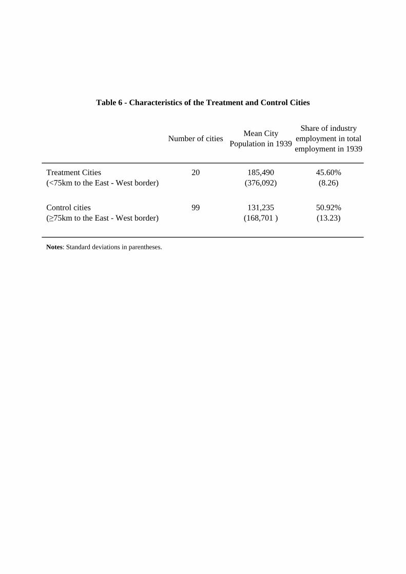
Number of citiesMean City

Population in 1939

Share of industry employment in total employment in 1939

Treatment Cities 20 185,490 45.60%(<75km to the East - West border) (376,092) (8.26)

Control cities 99 131,235 50.92%(≥75km to the East - West border) (168,701 ) (13.23)

Table 6 - Characteristics of the Treatment and Control Cities

Notes: Standard deviations in parentheses.

(1) (2) (3) (4)Population

GrowthPopulation

GrowthPopulation

GrowthPopulation

Growth

Border × Division -0.921*** -1.000*** -0.888*** -0.782***(0.218) (0.253) (0.247) (0.261)

Border 0.309* 0.338** 0.082 0.061(0.153) (0.156) (0.167) (0.194)


Matching on PopulationTotal

EmploymentEmployment in 28 sectors

Employment in 28 sectors

and geography


Table 7 - Matching

Notes: Left-hand side and right-hand side variables are defined as in Table 2. The years included are the same as in Table 2. In Column (1) matching is based on minimizing squared 1939 population differences between treatment and control cities. In Column (2) matching is based on minimizing squared 1939 employment differences between treatment and control cities. In Column (3) matching is based on minimizing the sum of squared 1939 employment differences in 28 sectors. In Column (4) matching is based on minimizing the sum of squared 1939 employment differences in 28 sectors and requiring the control city to lie within 100-175 kilometers from the East-West German border. Standard errors are heteroscedasticity robust and adjusted for clustering on city. * denotes significance at the 10% level; ** denotes significance at the 5% level; *** denotes significance at the 1% level.

(1) (2)Population

GrowthPopulation

Growth

Border × Division -0.737*** -0.656***(0.182) (0.191)

Border 0.136 0.129(0.139) (0.146)

War Devastation × Year 1919-25 -0.014 -0.004 (0.011) (0.006)

War Devastation × Year 1925-33 0.019 0.006(0.017) (0.007)

War Devastation × Year 1933-39 -0.001 0.004(0.023) (0.009)

War Devastation × Year 1950-60 0.073*** 0.033***(0.015) (0.008)


War Devastation × Year 1970-80 -0.014 0.004(0.025) (0.012)


Year Effects Yes Yes

Observations 777 756R-squared 0.24 0.24

Notes: Left-hand side and right-hand variables are defined as in Table 2 except for War Devastation. The years included are the same as in Table 2. In Column (1) War Devastation is measured as rubble per capita, expressed as cubic metres per capita. In Column (2) War Devastation is the number of destroyed dwellings as a percentage of the 1939 stock of dwellings. The war devastation variables are missing for a few cities which accounts for the smaller number of observations than in Table 2. Standard errors are heteroscedasticity robust and adjusted for clustering on city. * denotes significance at the 10% level; ** denotes significance at the 5% level; *** denotes significance at the 1% level.

Table 8 - War Devastation

(1) (2) (3)Population

GrowthPopulation

GrowthPopulation

Growth

Subsidy × Division -0.851*** -1.137*** -0.565**(0.179) (0.221) (0.225)

No Subsidy × Division -0.432 -0.487 -0.377 (0.374) (0.604) (0.244)

Subsidy 0.104 0.104 0.104(0.141) (0.141) (0.141)

No Subsidy 0.203 0.203 0.203(0.302) (0.302) (0.302)

Year Effects Yes Yes Yes

Year Sample1919-1939 &

1950-19881919-1939 &

1950-19701919-1939 &

1970-1988

Observations 833 595 595R-squared 0.21 0.10 0.21

Notes: Left-hand and right-hand side variables defined as in Table 2, except Subsidy is a dummy variable which equals one if a city is located within 75 kilometers of the border and qualifies for support under the Border Region Support Act 1971, and No Subsidy is a dummy variable which equals one if a city is located within 75 kilometers of the border and does not qualify for support under the Border Region Support Act. In Column (2) the division sample is restricted to the years 1950-70. In Column (3) the division sample is restricted to the years 1970-88. Standard errors are heteroscedasticity robust and adjusted for clustering on city. * denotes significance at the 10% level; ** denotes significance at the 5% level; *** denotes significance at the 1% level.

Table 9 - Subsidies

(1) (2) (3) (4)Population

GrowthPopulation

GrowthPopulation

GrowthPopulation

Growth

Border × Division -0.477*** -0.127 -0.223 -0.007 (0.156) (0.128) (0.202) (0.136)

Border -0.141 -0.141 -0.236 -0.064 (0.106) (0.106) (0.168) (0.108)


City Sample All All Small Cities Large Cities

Year Sample1950-1988 &

1992-2002 1980-1988 &

1992-2002 1980-1988 &

1992-20021980-1988 &

1992-2002


Table 10 - Reunification

Notes: Left and right-hand side variables are defined as in Table 2. In Column (1) population growth rates are for 1950-60, 1960-70, 1970-80, 1980-88, and 1992-2002. In Columns (2) to (4) population growth rates are for 1980-88 and 1992-2002. Column (3) reports results for small cities defined as those with a 1919 population below the median. Column (4) reports results for large cities defined as those with a 1919 population greater than or equal to the median. Standard errors are heteroscedasticity robust and adjusted for clustering on city. * denotes significance at the 10% level; ** denotes significance at the 5% level; *** denotes significance at the 1% level.

stephen redding london school of economics and …sticerd.lse.ac.uk/dps/pepp/pepp11.pdf · stephen...

Documents