steel-sandwich elements in long-span bridge applications

Department of Civil and Environmental Engineering Division of Structural Engineering Steel and Timber Structures CHALMERS UNIVERSITY OF TECHNOLOGY Gothenburg, Sweden 2016 Master’s Thesis BOMX02-16-21

Steel-Sandwich Elements in Long-Span Bridge Applications Master’s Thesis in the Master’s Programme Structural Engineering and Building Technology

EMMANOUIL ARVANITIS EVGENIOS PAPADOPOULOS

MASTER’S THESIS BOMX02-16-21

Steel-Sandwich Elements in Long-Span Bridge Applications

Master’s Thesis in the Master’s Programme Structural Engineering and Building Technology EMMANOUIL ARVANITIS

EVGENIOS PAPADOPOULOS

Department of Civil and Environmental Engineering

Division of Structural Engineering Steel and Timber Structures

CHALMERS UNIVERSITY OF TECHNOLOGY

Göteborg, Sweden 2016

I

Steel-Sandwich Elements in Long-Span Bridge Applications

Master’s Thesis in the Master’s Programme Structural Engineering and Building Technology EMMANOUIL ARVANITIS


© EMMANOUIL ARVANITIS, EVGENIOS PAPADOPOULOS 2015

Examensarbete BOMX02-16-21 Institutionen för bygg- och miljöteknik,

Chalmers tekniska högskola 2016


Division of Structural Engineering

Steel and Timber Structures

Chalmers University of Technology

SE-412 96 Göteborg

Sweden

Telephone: + 46 (0)31-772 1000

Cover:

Configuration of steel sandwich element as well as FE-model for the deflection analysis


Göteborg, Sweden, 2016

I

Steel-Sandwich Elements in Long-Span Bridge Applications Master’s thesis in the Master’s Programme Structural Engineering and Building Technology EMMANOUIL ARVANITIS



Division of Structural Engineering Steel and Timber Structures

Chalmers University of Technology

ABSTRACT

The aim of this Master Thesis project was to investigate and identify the quantity of

steel which could be saved if steel sandwich elements could be utilized in long span

bridge decks instead of conventional orthotropic plates. Therefore, after a literature

study about long span bridges and bridge decks, an optimization routine was created

which could optimize a steel sandwich element cross-section according to the desired

results. The scenarios studied in this Master Thesis project were the maximization of

the moment of inertia in the longitudinal direction, the minimization of the steel used

in the cross-section and the maximization of the length of the steel sandwich element

between two transverse stiffeners. As a reference bridge, Höga Kusten bridge was

chosen in order to compare the results. The scenarios had been studied in the

serviceability limit state taking into account the maximum global deflection that the

existing orthotropic deck of Höga Kusten bridge.

The results showed that steel sandwich elements could be provide a much lighter bridge

deck for long span bridges as far as the SLS is concerned. The plate behaviour of a steel

sandwich element enabled a better stress distribution in all directions that allowed less

material in the cross-sectional compared with the conventional orthotropic deck of

Höga Kusten bridge.

Key words: steel sandwich, orthotropic, plates, bridge deck

II

Stålsandwichelement i lång-span broapplikationer

Examensarbete inom masterprogrammet Structural Engineering and Building

Technology

EMMANOUIL ARVANITIS


Institutionen för bygg- och miljöteknik

Avdelningen för Avdelningsnamn

Forskargruppsnamn

Chalmers tekniska högskola

SAMMANFATTNING

Syftet för detta examensarbete var att undersöka och identifiera huruvida

stålsandwichelement kan nyttjas som brobaneplattor istället för konventionella

ortotropiska plattor för broar med stora spännviddar. Efter litteraturstudie skapades en

optimeringsrutin för stålsandwichelements tvärsnitt med avseende på tvärsnittsarea

eller yttröghetsmoment. Scenarierna som studerats i detta examensarbete var

maximeringen av tröghetsmomentet i längdriktningen, minimeringen av tvärsnittsarea

och maximeringen av längden av stålsandwichelement mellan två tväravstyvningar.

Som referensbro valdes Högakustenbron. Studierna utfördes med avseende på

brukgränstillståndet.

Resultaten visade att tillämpning av stålsandwichelement ger ett lättare brodäck för

broar med stora spinnviddar. Dessutom påvisades att viktreducering kan utnyttjas som

reducerad tvärsnittsarea eller ökat avstånd mellan tvärskott.

Nyckelord: stålsandwich, ortotropisk, plattor, brodäck

CHALMERS Civil and Environmental Engineering, Master’s Thesis BOMX02-16-21 1

Contents ABSTRACT I

SAMMANFATTNING II

CONTENTS 1

PREFACE 3

NOTATIONS 4

1 INTRODUCTION 6

1.1 Background 6

1.2 Scope of study 7

1.3 Aim and Objectives 7

1.4 Methodology 7

1.5 Limitations 7

1.6 Outline 8

2 LITERATURE STUDY 9

2.1 Suspension bridges 9 2.1.1 History 9

2.1.2 Structural system 10 2.1.3 Orthotropic steel decks 12 2.1.4 Box girder section 13 2.1.5 Stiffening girder 18 2.1.6 Shear lag effect 21 2.1.7 Local distortion mechanisms in bridge deck 22

2.2 Steel sandwich elements 24 2.2.1 Introduction 24 2.2.2 History 24

2.2.3 Corrugated core steel sandwich elements 25

3 HÖGA KUSTEN BRIDGE 28

3.1 The compression flange 29

3.2 Classification of the cross section 29

3.3 Axial load-carrying capacity 31

3.4 Deflection 32

4 OPTIMIZATION ANALYSIS 34

4.1 Introduction 34

4.2 Choice of the constraints 36

4.3 The studied scenarios 38

CHALMERS, Civil and Environmental Engineering, Master’s Thesis BOMX02-16-21 2

4.3.1 Maximization of the moment of inertia in the longitudinal direction 38 4.3.2 Minimizing the material used 38 4.3.3 Minimizing the area by adding a longitudinal stiffener 39 4.3.4 Maximizing the length between the transverse stiffeners 39

4.4 Finite Element Analysis 39

5 RESULTS 41

5.1 Study 1 - Maximization of the moment of inertia in the longitudinal direction

41

5.2 Study 2 - Minimization of the material used 41

5.3 Study 3 - Minimizing the material used by adding a longitudinal stiffener 49

5.4 Study 4 - Maximizing the length between the transverse stiffeners 53

5.5 Verification of the deflection 54

5.6 Moment and axial capacity 56

6 DISCUSSION 60


60

6.2 Study 2 - Minimization of the material used 60

6.3 Study 3 - Minimizing the material used by adding a longitudinal stiffener 60

6.4 Study 4 - Maximizing the length between the transverse stiffeners 61

7 CONCLUSIONS 62

8 REFERENCES 63

9 APPENDIX A

10 APPENDIX B


Preface This Master Thesis was performed in order to investigate the possibility of using steel

sandwich bridge decks in long-span bridge applications. The study took place from

January to June 2015 and it was performed in collaboration with WSP. The project was

carried out at the Department of Structural Engineering, Steel and Timber Structures,

Chalmers University of Technology, Sweden.

The authors would like to thank their supervisor Peter Nilsson, as well as their examiner

Mohammad Al-Emrani for their guidance and support. They would also like to thank

Amanda Palmkvist and Linda Sandberg for the excellent opposition.

Göteborg June 2016

Emmanouil Arvanitis & Evgenios Papadopoulos


Notations Roman upper case letters

CSC Cross section class

FEM Finite Element Method

HLAW Hybrid laser arc welding

OSD Orthotropic steel deck

SLS Serviceability limit state

SS Steel sandwich

SSE Steel sandwich element

Roman lower case letters

f Closest distance between the stiffeners of the core

h Height of the steel sandwich element

hc Height of the core of the steel sandwich element

p Half length of the core repetition

tf.top Thickness of the top plate

tf.bot Thickness of the bottom plate

tc Thickness of the corrugated core

Greek lower case letters

α Angle of the core stiffeners with the horizontal axis


1 Introduction 1.1 Background In the summer of 2010, the Norwegian Public Road Administration (NPRA) decided to

initiate a project for a coastal trunk road that will start from Trondheim, in the middle

of Norway, pass along the western corridor (E39) and end in Kristiansand, in the south

part of the country. The purpose for the update of this 1330 km highway is to facilitate

the trade and industry transportation in the south-western Norway, which is still

hampered by the wide and deep fjord crossings. At the present time, the traffic

connection in many points is accomplished by ferry boats. This increases the travel time

needed between the cities in the area. The NPRA want to create an effective

transportation system in the whole western region as it interconnects areas with large

populations and substantial trade and industry; E39 is the most crucial route of this

vision. For the construction of E39, various technological alternatives are examined for

bridging the fjord crossings still being operated by ferry boats. The proposals include

new innovative concepts for structural systems, construction methods and materials.

Many of the fjord crossings in Norway are difficult and expensive to be bridged.

Particularly Sognefjord, possessing a width of 4km and a depth that reaches 1500m in

some locations, is an extremely challenging passing. In the attempt of bridging longer

spans with cable bridges, the construction of lighter and stiffer bridge decks is a

necessary parameter. Nowadays, the most common deck structure is the orthotropic

steel deck, consist of a steel plate stiffened by longitudinal open or closed ribs.

However, orthotropic decks suffer from many disadvantages, such as poor fatigue

performance and high production costs.

To counteract these problems steel sandwich elements (SSE) has been proposed to

replace the conventional orthotropic bridge deck. SSE are light-weight construction

elements consist of two thin face sheets connected by a core, which can be

manufactured with different configurations (Beneus & Koc 2014). Their high stiffness

to weight ratio has made them a considered solution in the shipbuilding and aerospace

industry and some implementations have been performed (Roland & Reinert 2000).

Moreover, new innovative technics, concerning laser welding, increased their fatigue

performance and enabled industrialized manufacture. Today more and more efforts and

research are made for the integration of these elements in bridge engineering in order

to exploit all their advantages.

A box girder cross section is typically a rectangular or trapezoidal box, which is used

for large scale structures and can be constructed with various materials and techniques.

The box girders are a quite popular choice in the bridge engineering industry, mainly

due to their high torsional stiffness (Xanthakos 1993). Moreover, this kind of cross-

section enables much longer spans, while it also possesses other advantages like

uncomplicated maintenance and visual aesthetics. Box girder cross-sections are mostly

used in beam bridges and suspension bridges.

By combining SSE with box girder sections and exploiting their assets, new light-

weight box-girders could be created. These box girder cross sections could be used to

enable longer bridge spans in a more cost-efficient way.


1.2 Scope of study The scope of this study is to investigate if it is possible to achieve an essential goal of

the bridge industry; to decrease the self-weight of the structural elements of the bridge.

Nowadays, researchers are examining the use of light-weight materials and structural

elements, which would minimize the construction cost and reduce our CO2 footprint.

As welding technology advances, SSEs have shown great potential for bridge deck

applications. Furthermore, although there is a broad bibliography on SSEs, there is no

similar study done, where the SSEs have been combined with the box girder cross-

section.

1.3 Aim and Objectives The purpose of the Master Thesis project is the development of a cross-section that

would utilize the advantages of the two mentioned systems, the box girder cross section

and the SSE. This can make it possible to create lighter and more efficient stiffening

girders for long-span bridge applications. The structural behaviour of the steel deck, for

instance strength and stiffness parameters, was decided in accordance with the

Eurocode 3 using numerical analysis. The specific objectives of the project are:

• Evaluation of the application of SSE in long-span bridges

• Design of SSE which are optimum for different cases with respect to SLS

• Design comparison in a case study

1.4 Methodology To accomplish the objectives, the steps below were followed:

• Literature study on suspension bridges

• Literature study on box girder section

• Literature study on structural behaviour of steel sandwich bridge decks

• Calculation of load-carrying capacities of the compressive flange of an existing

box girder section (Höga Kusten Bridge)

• Calculation of load-carrying capacities of an optimized SSE

• Comparison between the conventional section and SSE cross-section

1.5 Limitations The Master Thesis project will be focused on the investigation of the structural

behaviour and design of SSE for suspension bridge applications. Although, fatigue has

been shown to be a crucial aspect in such constructions, it is not examined in the specific

project. The centre of attraction of this project will be the structural behaviour of the

stiffening girder and not the behaviour of the entire bridge.

Although there are many different core configurations when using SSE, for the needs

of the specific project, corrugated core SSE will be used. With respect to manufacturing

and structural performance this core type has been shown to be a suitable option for

bridge deck applications (Beneus & Koc 2014).

The comparison between the orthotropic section and the one utilizing SSE will be based

on the existing bridge geometry. In other words, the positions of the stiffeners will be

the same with those of the existing bridge.


1.6 Outline The Master Thesis project will be focused on the investigation of the structural

behaviour and design of SSE for suspension bridge applications. Although, fatigue has

been proven to be a crucial aspect in such constructions, it is not examined in the

specific project. The centre of attraction of this project will be the structural behaviour

of the stiffening girder and not the behaviour of the entire bridge.

Although there are many different core configurations when using SSE, for the needs

of the specific project, corrugated SSE will be used. This is due to the fact that the

specific configuration can result in light elements, with high bending and shear stiffness

in both directions, i.e. a low level of orthotropy. Furthermore, the production of this

element type is feasible.

The comparison between the orthotropic section and the one utilizing SSE will be based

on the existing bridge geometry. In other words, the positions of the stiffeners will be

the same with those of the existing bridge.


2 Literature Study 2.1 Suspension bridges 2.1.1 History Suspension bridges have been used to overcome large spans for almost two hundred

years. Since new technologies were adapted and construction processes improved, the

covered main span lengths were continuously increased over the years, to reach a

maximum distance of approximately 2.000 meters nowadays (Gimsing & Georgakis

2012).

The main principle behind the function of suspension bridges, and suspension systems

in general, is the utilization of tensile elements for the load transfer. This principle has

been used since ancient times, when the ancient Chinese used ropes and iron chains to

overcome river spans 2.000 years ago (Xu & Xia 2011).

The first suspension bridge in the United States was built in the state of Pennsylvania

in 1796 by James Finley and it was named Jacob's Creek Bridge (Xanthakos 1993).

Jacob's Creek Bridge used wrought iron chains and a level deck to connect Uniontown

to Greensburg, see Figure 2.1. Its main span was 21 m long and 3.81 m wide (Finley

1810). In Europe, the first permanent suspension bridge was built in 1823 in Geneva

by Marc Seguin and Guillaume-Henri Dufour. It was the Saint Antoine Bridge, which

had two equal spans of 42 m (Peters 1980). In the 19th century many suspension bridges

were constructed, with pin-connected eye-bars forming huge chains, being the main

load-carrying elements (Gimsing & Georgakis 2012). A characteristic example of this

bridge type is the Clifton Suspension Bridge in Bristol, United Kingdom, which was

designed by Isambard Kingdom Brunel and opened in 1864.

Figure 2.1 Jacob's Creek Bridge, the first suspension bridge in the United States (Finley 1810).

The first modern suspension bridge is considered to be the Brooklyn Bridge across the

East river between Manhattan and Long Island in the New York, United States. The

construction of Brooklyn Bridge started in 1867 under the supervision of John

Roebling, who was the main designer, and it opened to traffic in 1883. In the

meanwhile, John Roebling died and the construction was taken over by his son

Washington. The Brooklyn Bridge had a main span of 486 m and two side spans of 286


m and at the time that it opened, it was 50% longer than the previously built bridges

(Gimsing & Georgakis 2012).

2.1.2 Structural system The typical configuration of a suspension bridge is shown in Figure 2.2. The bridge is

mainly composed by the stiffening girder with the bridge deck, the cable system, the

pylons and the anchor blocks. The pylons support the cable system, which in turn

supports the stiffening girder. The anchor blocks stabilize the cable system vertically

and horizontally.

Figure 2.2 Suspension bridge with its main components (Gimsing & Georgakis

2012).

The side span lengths are usually between 0.2-0.5 times the main span, as shown in

Figure 2.2 (Gimsing & Georgakis 2012). However, depending on the on-site conditions

of the bridge, the length of the side spans may differ. For instance, if the side spans of

the bridge have to be placed over deep water, long side spans are usually preferred, to

avoid complicated support systems of the pylons in the water. On the other hand, if the

supporting pylons are placed on land or in shallow water, short side spans can be

chosen.

Cable bridges can be characterized depending by the way the cable system is anchored.

There are two anchorage systems; the earth and the self-anchored. In the former both

the vertical and the horizontal components of the cable force are transferred to the

anchor block, whereas in the latter the horizontal component is transferred to the

stiffening girder, see Figures 2.3 and 2.4. Although both anchorage systems can be

used, earth anchorage system is mostly used. This is due to the fact that self-anchoring

suffers from low structural efficiency and construct-ability, resulting in uneconomical

configurations (Gimsing & Georgakis 2012).

Figure 2.3 Self-anchorage system (left) and earth anchorage system (right) (Gimsing & Georgakis 2012).


Figure 2.4 Self anchorage system (top) and earth anchorage system (bottom) (Gimsing & Georgakis 2012).

As far as the cable arrangement in the transverse direction is concerned, there are plenty

of solutions; the most common is the one shown in the Figure 2.5, where the cables

support the deck in the two edges. This arrangement provides adequate vertical

stability, as well as additional torsional stiffness. Depending on the expected loading

conditions and the design of the bridge, other configurations are also possible, see

Figure 2.6.

Figure 2.5 Vertical cable planes attached along the edges of the deck (Gimsing &

Georgakis 2012).

Figure 2.6 Various cable configurations in the transverse direction (Gimsing &

Georgakis 2012).

The choice of the support conditions is the most significant factor regarding the

structural behaviour of the stiffening girder. For the most simple and frequently used

three-span suspension bridge, the stiffening girder often consists of three girders,

simply supported at the pylons and longitudinally fixed at the anchor blocks (Figure

2.7).


Figure 2.7 Supporting conditions in three-span suspension bridge (Gimsing &

Georgakis 2012)

It should be noted that in this case, the support conditions are favourable regarding

deformations caused by temperature changes, because the maximum longitudinal

displacements will occur next to the pylons, where the hangers have their maximum

length. Consequently, the change of the inclination of the hangers will be as low as

possible (Gimsing & Georgakis 2012).

Another configuration for the stiffening girder is to be continuous all over the length of

the bridge. A continuous girder will result in a lower value of the maximum moments

compared with the simply supported option. However, special treatment is needed

because the bottom flange of the deck will be in compression close to the pylons. An

example of a configuration with continuous girder is shown in Figure 2.8. In this case,

special treatment would be needed because the maximum longitudinal displacement

due to temperature changes is longer than the three-span suspension bridge. In addition,

the maximum longitudinal displacement due to temperature changes and asymmetric

traffic loads will occur near the ends of the side spans. In this position the vertical

hangers have their minimum length and consequently their inclination will be the

maximum.

Figure 2.8 Continuous bridge deck longitudinally fixed at one pylon (Gimsing &

Georgakis 2012).

2.1.3 Orthotropic steel decks Modern steel bridges use the orthotropic deck system, in order to distribute traffic loads

over the structure, as well as to strengthen the slender plate elements under

compression. Compared with reinforced concrete decks, the Orthotropic Steel Decks

(OSDs) are lighter and therefore they can cover larger spans. The most common

configuration of an OSD consists of a flat, thin steel plate, stiffened by transverse floor

beams or diaphragms and longitudinal ribs, which can be either of closed or open type,

see Figure 2.9. The selection of the rib type affects the torsional rigidity of the section.

The closed are advantageous compared to the open ones. Due to this configuration, the

properties of an OSD vary in longitudinal and transverse direction. The longitudinal

direction is much stiffer, i.e. the level of orthotropy is high. A typical configuration of

an OSD, utilized in a box section girder, is shown in Figure 2.10.


.

Figure 2.9 Types of longitudinal ribs(Chen & Duan 2014).

Figure 2.10 General structure of box section girder with orthotropic steel bridge deck (Chen & Duan 2014).

The main reason for utilization of OSD bridges is that they have high stiffness to weight

ratio. Moreover, the application of OSD solutions results in structures made wholly of

steel with high degree of standardization in the design. On the other hand, the behaviour

of OSD with regard to fatigue is considered to be problematic, since fatigue cracking is

a common problem in such decks due to the complicated welded details (Lebet & Hirt

2013).

2.1.4 Box girder section The box girder section is often used in steel-bridge structures due to the high

performance regarding torsional stiffness. Moreover, using box girders can result in

improved durability compared to open sections, due to the fact that a large proportion

of the steel is not exposed. In addition, box girder sections are advantageous regarding

the erection of bridges, as they are more suitable for the cantilevering method and they

present smaller deformations during the erection. On the other hand, the main

Flat plate rib Bulb plate rib U rib Trough rib

Open ribs Closed ribs


disadvantage when choosing box girder sections is the increased cost (Xanthakos

1993).

The distortion of a box girder under the effect of eccentric loading is shown in Figure

2.11a. Figure 2.11b shows the transverse bending moments due to out-of-plane flexure

of the plates and Figure 2.11c shows the longitudinal stresses due to in-plane bending

(Hambly 1991).

Figure 2.11 (a) Distortion of box girder; (b) out-of-plane bending moments; (c) in-plane bending (warping) stresses (Hambly 1991).

Figure 2.12 shows how distortion forces develop in box girders. The warping constant

is assumed to be zero and consequently the stresses based on the thin walled beam

theory response are very small. As a result, the distortion of the box girder leads to

important plate bending and normal stresses.

Figure 2.12 Stresses in box-section under eccentric load (US Department of

Transportation 2012b).


To show analytically the development of the distortion forces in a box girder, the

eccentric load in Figure 2.13 can be divided in two loads, a symmetric and an

antisymmetric. The symmetric component results to vertical bending of the box-girder.

The antisymmetric load cannot be directly linked with torsion on the box, since pure

torsion includes a system of shear flows round the cell as shown in Figure 2.13e, so it

is redrawn and it results in the combination of pure torsion shear flows and distortion

shear flows as shown in Figure 2.13d. The torque involved in the pure torsion (Figure

2.13e) is equal to the torque of the antisymmetric loading (Figure 2.13d). The distortion

shear flows in Figure 2.13f are self-balanced and have no net resultant but at the same

time they cause distortion of the cell as shown in Figure 2.13c. The box girder section

is very stiff in pure torsion and most of the twist is due to distortion. Therefore, cross

bracing is needed to reduce the distortion effects and this is why vertical beams are used

in box girders (Hambly 1991).

Figure 2.13 Distortion forces in box girders (Hambly 1991).

In some cases, a box girder element underlain to torque is going to present also warping

stresses. Moreover, every wall element will obtain some shear deformation to establish

the continuity of axial displacements in the perimeter. The warping distribution does

not remain the same in every section of the beam, due to the varying torsional moment

and the different form along the span.


Figure 2.14 Warping Torsion in box girder element.

The structural analysis of a box girder bridge, which is subjected to external load, can

be simplified by studying a beam located at the centre of gravity of the box girder

(Figure 2.15). For this simplification to be valid, the following conditions must be

satisfied:

• The length of the beam must be considerably greater than the cross section

dimensions

• The cross section must not distort because of beam deflections

• Shear deflections are negligible

• Stresses are proportional to deformations

In order to satisfy the 2nd condition, cross bracing is needed as already mentioned.

Figure 2.15 Modelling of the bridge (Lebet & Hirt 2013).

The structural analysis of a bridge includes the calculation of its internal section forces

due to the external load. To show analytically how the internal moments are calculated,

an example of a bridge with box girder cross section will be used. As shown in the

Figure 2.16, the bridge is subjected to the vertical load qz and the horizontal load qy.


With the assumption of linear elastic behaviour, the internal moments and forces are

resolved about the shear centre CT and bending is caused. Moreover, if the loads do

pass through the shear centre CT, a torque mT will develop on the beam, as shown in

the Figure 2.17. This torque causes torsional moments Mx about the x axis.

Then the structural analysis can be carried out, with the calculation of the bending

moments and shear forces, as well as the torsional moments. It should be noted that the

choice of the restraints depends on the type of bearings, as well as on the type of piers.

The calculation of the internal moments and forces through the above steps is shown in

the Figure 2.18.

The simplified analysis is valid only if the required conditions are satisfied. In case that

these conditions are not fulfilled, the three dimensional behaviour of the bridge should

be considered; for instance when the local effects are of the same magnitude with the

global effects, more complex analyses are required.

Figure 2.16 Actions on the bridge.

Figure 2.17 Analysis of the forces acting on the cross-section.

2b

h

qz

qy

y

z

yq

qz·b

h/2

zq

qy·h

qz·b

CTqy·hCT

mT=qz·b·yq+qy·h·zq

= =


Figure 2.18 Internal moments and forces along the x axis (Lebet & Hirt 2013).

2.1.5 Stiffening girder The stiffening girder of a suspension bridge is the structural component which is

subjected to the largest proportion of the external load. This is due to the fact that the

traffic load is applied directly to it. Moreover, the self-weight and the wind loads are

usually larger for the stiffening girder than for the cable system. Therefore, the

stiffening girder must be able to withstand all the global stresses created by its self-

weight and the variable loads, redistribute them and transfer them to the cables. In

addition, it should have sufficient flexural rigidity to resist the local stresses between

the hangers. It should also possess enough torsional stiffness to resist the torsional

stresses induced by eccentric loading and wind. The axial stiffness is normally not of

importance for suspension bridges, because the hangers are vertical. Thus, there is no

horizontal component induced.

Regarding the stiffness against vertical loads, the stiffening girder should at least be

able to resist the loads between the hangers. This is the local scale of the loading. For

the global resistance, the stiffening girder will be assisted by the cable system to carry

the load and transfer it at the supports.

The stiffening girder should also have sufficient resistance against lateral loads. In this

direction there is no assistance from the cable system. Therefore, it is preferable to have

a continuous bridge stiffening girder, so that the total moment would be distributed

between the positive moment in the span and the negative moment at the pylons, see

Figure 2.19.


Figure 2.19 Transverse moment distribution with different approaches in the bridge stiffening girder (Gimsing & Georgakis 2012)

When lateral or transverse load acting on the stiffening girder is not passing through

the shear centre of the beam - shear centre is defined as the point which shear loads do

not cause twist - apart from bending, twisting will occur as well. When an element is

symmetrical to all three directions, then the shear centre is located in the centre of the

element. Likewise, if the element has a cross section symmetrical to two directions,

then the shear centre is on the centre of the cross section, while if it is has just a

symmetry axis then the shear centre is moving on that symmetry axis.

The result of a load, eccentric to the shear centre acting on the element, is double; apart

from twisting, warping will take place as well. Warping is the phenomenon of torsion

that does not permit a twisting plane section to remain plane while rotating. Warping

can be considered as the second effect of torsional loading. If a cross-section can

elongate freely, then warping does not induce stresses. This is known as free warping.

Otherwise, the warping torsion is added to the uniform torsion to counterbalance the

torque and is referred as non-uniform torsion. In this case, apart from shear stresses,

axial stresses are induced, as shown in the Figure 2.20.

Figure 2.20 Non uniform torsion: Prevented end warping deters free twisting (Institute for Steel Development & Growth 1999).

Non-uniform torsional resistance is generally the sum of two phenomena; St. Venant’s torsion (also referred as pure torsion) and warping torsion. The major parameters

affecting the non-uniform torsional rigidity are the properties of the material, the length


of the member, the dimensions of the cross sections and the supporting conditions.

Some examples are presented in the Figure 2.21 below.

Figure 2.21 Examples of pure and warping torsion in simply supported beams and

cantilevers (Institute for Steel Development & Growth 1999).

In cable bridges, the required torsional stiffness of the stiffening girder is highly

dependent on the choice of the cable system. A suspension bridge with a cable system

centrally placed in the transverse direction requires a more torsional rigid stiffening

girder, in relation to a bridge with two cable planes on the edges. Generally, the torsion

is governed by the number and the configuration of the cable planes.

The torsional moment of a vertical eccentric load can be sustained either by the

stiffening girder or by the cables or a combination of them, as show in the Figure 2.22.

The torsion taken from the stiffening girder is imported in the section by the parallel

action of two components, see Figure 2.23. In the first one a linear distribution of the

shear stresses along the thickness is noticed, while in the second the shear distribution

remains constant along the thickness of different components. However, most of the

times the former is small compared to the latter and therefore is neglected. Similar

behaviour is also expected for loads parallel to the bridge stiffening girder such as wind,

earthquake, etc.

Figure 2.22 Various ways of carrying an eccentric load depending on the torsional stiffness and the cable system (Gimsing & Georgakis 2012).


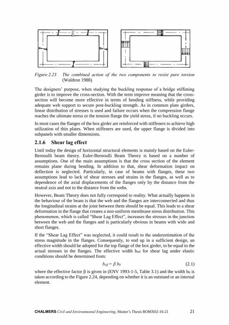
Figure 2.23 The combined action of the two components to resist pure torsion (Waldron 1988).

The designers’ purpose, when studying the buckling response of a bridge stiffening girder is to improve the cross-section. With the term improve meaning that the cross-

section will become more effective in terms of bending stiffness, while providing

adequate web support to secure post-buckling strength. As in common plate girders,

linear distribution of stresses is used and failure occurs when the compression flange

reaches the ultimate stress or the tension flange the yield stress, if no buckling occurs.

In most cases the flanges of the box girder are reinforced with stiffeners to achieve high

utilization of thin plates. When stiffeners are used, the upper flange is divided into

subpanels with smaller dimensions.

2.1.6 Shear lag effect Until today the design of horizontal structural elements is mainly based on the Euler-

Bernoulli beam theory. Euler-Bernoulli Beam Theory is based on a number of

assumptions. One of the main assumptions is that the cross section of the element

remains plane during bending. In addition to that, shear deformation impact on

deflection is neglected. Particularly, in case of beams with flanges, these two

assumptions lead to lack of shear stresses and strains in the flanges, as well as to

dependence of the axial displacements of the flanges only by the distance from the

neutral axis and not to the distance from the webs.

However, Beam Theory does not fully correspond to reality. What actually happens in

the behaviour of the beam is that the web and the flanges are interconnected and thus

the longitudinal strains at the joint between them should be equal. This leads to a shear

deformation in the flange that creates a non-uniform membrane stress distribution. This

phenomenon, which is called “Shear Lag Effect”, increases the stresses in the junction between the web and the flanges and is particularly obvious in beams with wide and

short flanges.

If the “Shear Lag Effect” was neglected, it could result to the underestimation of the stress magnitude in the flanges. Consequently, to end up in a sufficient design, an

effective width should be adopted for the top flange of the box girder, to be equal to the

actual stresses in the flanges. The effective width beff for shear lag under elastic

conditions should be determined from:

beff = β b0 (2.1) where the effective factor β is given in (ENV 1993-1-5, Table 3.1) and the width b0 is

taken according to the Figure 2.24, depending on whether it is an outstand or an internal

element.


Figure 2.24 Notations for shear lag (ENV 1993-1-5).

beff is the effective part of the flange under uniform stress is in equilibrium with the

actual non-uniform stress distribution.

2.1.7 Local distortion mechanisms in bridge deck The action of the wheel loads in the bridge deck is responsible for a series of local

deformation which are shown on Table 2.1 and discussed below.


Table 2.1 Orthotropic steel deck deformation mechanisms (US Department of

Transportation 2012a).

In system 1 the wheel loads are transferred from the deck plate to the supporting ribs.

The decisive factors for this response are the relative thickness of the deck plate and

the ribs, as well as the spacing of the ribs. This action can cause fatigue failure in the

connection between the ribs and the deck plate, but in most cases it is not crucial for

strength based limit states.

System 2 represents the deformation of the deck panel under out-of-plane loading

which results in transverse deck stresses due to the differential displacements of the

System Action Figure

1

Local Deck

Plate

Deformation

2Panel

Deformation

3

Rib

Longitudinal

Flexure

4Floorbeam In-

plane Flexure

5Floorbeam

Distortion

6 Rib Distortion

7 Global

Diaphragm curvature

between ribs

Diaphragm curvature

at bottom of the rib

Wheel load

Stiffener

Deck plate

Detail A

Mb

Detail A

MdMb + Md

Detail A Wheel load

Wheel load

P

Deflection line

F2F1

F0

F2F1

F0

Wheel load


ribs. This system is the most complicated to analyse due to the two-way load

distribution of the OSD panel. Furthermore, its behaviour is further affected by the type

of the ribs.

System 3 represents the behaviour of the ribs in their longitudinal direction. After the

load distribution in the transverse direction as described in system 2, the ribs transfer

the load in the longitudinal direction to the transverse beams of the girder. The ribs are

considered as continuous beams on discrete flexible supports which represent the

transverse beams.

Systems 4 and 5 are used to show the mechanisms which are developed during the

transference of the loads from the ribs to the girders through the transverse beams. The

transverse beams act as beams between rigid girders and the stresses that develop are

due to combination of in-plane stress (flexure and shear) and out-of-plane stress

(twisting) from rib rotation. System 4 describes the former, whilst system 5 describes

the latter.

System 6 corresponds to the rotation of the rib in a closed-rib system, when the wheel

load is at the mid-span and acts eccentric to the axis of the rib. In such loading cases,

the rib twists about its centre of rotation and results in lateral displacement at the mid-

span.

Finally, the 7th system describes the behaviour of the primary girder between the global

supports and the resulting axial, shear and flexural stresses due to the deformations (US

Department of Transportation 2012a).

2.2 Steel sandwich elements 2.2.1 Introduction Throughout the centuries, the constant need for bigger, lighter and more durable

constructions has pushed researchers to pursue solutions for innovative materials, new

structural systems and high performance elements to achieve their most ambitious

visions. Structural steel was always an outstanding choice for meeting these

expectations as it provides a variety of advantages; high strength to weight ratio,

durability, versatility, low cost and sustainability etc. In a continuous attempt for

exploiting these assets, engineers came up with new configurations; used for different

applications. Steel sandwich elements are considered the state of art of this endeavour,

especially after new welding techniques came to limelight. The sandwich plates

considered in this Thesis consist of a corrugated plate fastened between two face plates,

see Figure 2.26.

2.2.2 History Although sandwich elements became more well-known after the second half of the 20th

century, evidences show their existence since 1849, when they were mentioned in the

texts of Sir William Fairbairn (Sir William Fairbairn 1849). The first proven sandwich

application though, was made of wood and it was shown in the ’Mosquito’ aircraft in

1940s (Vinson 1999). This is considered as the beginning of using sandwich elements

in the marine and aerospace industry. Until now, a variety of difficulties connected to

the manufacturing caused SSE limited utilization. Particularly, welding process was

making the total procedure relatively slow and expensive. Moreover, the lack of


knowledge about their long-term behaviour was the main reason that made engineers

sceptical about their field of application (Wolchuk 1990).

The last 20 years, steel sandwich panels began to enter drastically to the civil and

mechanical engineering industry. The main reason why this has happened is laser

welding, which has replaced the previous conventional spot-welding. Laser welding

techniques, and especially the combination of laser and gas metal arc welding into a

hybrid welding process, were proven to be a viable (Roland et al. 2004). HLAW

minimizes the part distortion and increases the accuracy, while the welding time can be

10 times faster than common welding methods (Blomquist et al. 2004). Furthermore, it

provides control of the geometric parameters of the welds and temperature variation,

high connection quality and excellent surface finish reducing the fairing and fitting

work in outfitting (Olsen 2009).

Figure 2.25 Production of SSE with HLAW (http://www.esab.com).

The application of SSE can result in a series of advantages but these can be summarized

in the following:

High stiffness to weight ratio

Low level of orthotropy

Industrialized construction process

Laser welded SSE can save approximately 30-50% of material compared with

conventional steel members (Kujala & Klanac 2005); fact that enables them to be an

economical solution in terms of manufacturing and transportation. The areas of their

application are extremely wide, extending from the marine, aerospace and offshore

industry to wind turbine blades, hoods, hatches, lift floors and bridge decks lately.

2.2.3 Corrugated core steel sandwich elements The steel sandwich elements can be divided into two big categories: elements with steel

faces bonded with an elastomeric core and elements with both faces and core made of

steel welded together. The latter includes steel cores that can be manufactured in

various shapes depending on the type of application. In this specific Master Thesis

project, the steel sandwich element studied has a corrugated core, as shown in the

Figure 2.26. A typical section of this type of elements, along with its characteristics, is

shown in the Figure 2.27. The reason why this type of SSE was examined, is because

it has been shown to be suitable for bridge decks(Beneus & Koc 2014).


Figure 2.26 Corrugated core SSE.

Taking into account that the steel core of the sandwich has different configuration in

the two main axes, it is obvious that the element possesses a strong and a weak direction.

Strong is called the direction where the flexural and shear rigidity is higher; the other

direction is the weak one lacking mainly in shear stiffness. In such a formation, the

function of the top and bottom plates is focused on the resistance to the bending

moments, while the core transmits shear forces. To model the behaviour of the SSE,

the Reissner-Mindlin plate theory can be applied, in order to transform the 3D sandwich

element to an equivalent 2D plate, see figure 2.27. This plate will have the elastic

constants that describe the behaviour of the SSE, see chapter 4.4.

Figure 2. 27 The principle of homogenization of the core properties.


Figure 2.28 Typical section of corrugated core SSE.

The variables, which characterize such a structural system (Figure 2.28), are:

the length between the core repetition, 2p

the height of the core, hc

the thickness of the top plate, tf.top

the thickness of the bottom plate, tf.bot

the thickness of the corrugated core, tc

the angle of the core stiffeners with the horizontal axis, α

the horizontal distance between two stiffeners, f

hc

f tf,bot

tf,top

tc

á

2p l


3 Höga Kusten Bridge Höga Kusten bridge, illustrated in Figures 3.1 and 3.2, is a suspension bridge located

in northern Sweden, between the municipalities of Härnösand and Kramfors. The

bridge was constructed in 1997 to connect the banks of Ångerman River and replace

the previously existing Sandö Bridge in the main road connection. The total length and

width of the bridge comes to 1867 and 22 meters respectively, while the height of the

two pylons holding the main cables extends more than 180 meters (Structurae.net,

2015). The long span of the bridge ranks it 3rd in Scandinavia and 4th in Europe among

the longest suspension bridges. The construction period was almost 4 years.

Figure 3.1 Höga Kusten bridge (http://www.bridge-info.org).

Figure 3. 2 Höga Kusten bridge (http://www.hogakustenstugor.se).


The cross section of the Höga Kusten bridge was chosen to be studied for this Master

Thesis project. This is due to the fact that it is one of the two suspension bridges located

in Sweden; the other one is the Älvsborg bridge. In addition to this, it is the only one

combining the box girder cross-section with a suspension system.

3.1 The compression flange The compression flange of the box girder is composed by a plate which is stiffened

longitudinally by stiffeners of closed type. The stiffened compression flange is

composed by several continuous beams, supported at the diaphragms. The compression

flanges may be subjected to the following stresses:

i) Longitudinal stresses caused by the global bending moment on the main girder.

ii) In-plane shear stress in the flange plate caused by local shear forces and torsion.

iii) Flexural stresses in the stiffeners caused by the local loads on the deck.

iv) In-plane transverse stresses in the flange plate caused by the bending of the

transverse flange stiffeners and the distortion of the box girder section.

Regardless of the stressing field mentioned above, a series of geometrical complexities

have to be investigated as well. These are:

i) The longitudinal continuity over the transverse stiffeners.

ii) The transverse continuity between parallel stiffeners.

iii) The different buckling modes.

iv) Geometrical imperfections and residual stresses in the flange plate and the

stiffeners.

Critical for the compression flange is the interaction between local buckling and global

buckling. This phenomenon can lead to rapid loss of the load resistance. Therefore, the

design codes for stiffened plate define the geometrical limitations which are not prone

to buckling and have no initial imperfections.

3.2 Classification of the cross section Initially, the orthotropic plate used for the bridge deck was checked with reference to

local buckling. The cross-section is composed by four parts, each of which has been

studied as individual plate. The slenderness ratio of each part has been calculated to

define the rotational capacity and check the sensitivity with regards to local buckling.

The clear dimensions were specified as the dimension of the middle lines minus the

thicknesses of the parts, as shown in Figure 3.3. The unit studied is part of the top plate

of the total box girder cross-section, which is principally subjected to uniform

compression in the middle span of the bridge.


Figure 3.3 Cross-section of the two units.

After defining the width to thickness ratios for the different components of the

compression flange, it was proven that the top and bottom horizontal parts belong to

Class 1. Therefore, their whole cross-sectional area can be used in the design, as they

can form plastic hinges in a statically indeterminate system. However, the webs of the

stiffener have a high slenderness ratio and therefore local buckling can take place before

yielding. These parts, which are classified in the 4th category, do not use their whole

cross-section regarding the moment and load carrying resistance, i.e. an effective cross-

section should be calculated. The classification and the effective area of each unit are

illustrated in Figures 3.4 and 3.5 respectively. Finally, the end parts in the edges of the

top plate were also classified in Class 1.

Figure 3.4 Classification of different parts.

Figure 3.5 Effective areas and gravity centre of the cross-section.

12

mm

306,2 mm

600 mm

293,8 mm

156,3 mm

30

4 m

m

313,1

mm

8 mm

21

9 m

m8

5 m

m6

7 m

m

Gravity centre of the

section

Gravity centre

of the webs

Gravity centre of

the bottom flange

Gravity centre

of the top flange

Class 1

Class 1

Class 1

Class 4


3.3 Axial load-carrying capacity For defining the moment capacity, the interaction between the column-type and the

plate-type buckling of the deck has to be studied. From the individual reduction factors

for each case, a final reduction factor will be obtained according to the following

equation (EN 1993-1-5):

𝜌𝑐 = (𝜌 − 𝜒𝑐)𝜉(2 − 𝜉) + 𝜒𝑐 (3.1)

where 𝜉 =𝜎𝑐𝑟.𝑝

𝜎𝑐𝑟.𝑐− 1 but 0 ≤ 𝜉 ≤ 1

σcr,p is the elastic critical plate buckling stress

σcr,c is the elastic critical column buckling stress

χc is the reduction factor due to column buckling

ρ is the reduction factor due to plate buckling

According to the drawings, the distance between the diaphragms was 4 m. The bridge

deck is subjected to uniform compression, see Figure 3.6. The normal compressive

stresses vary along the depth of each unit, as shown in Figure 3.7. To calculate the

distribution of the stresses, the neutral axis of the whole section, as well as the neutral

axis of the top plate has been defined. The centre of gravity was defined from the bottom

flange of the bridge deck, taking into consideration the position of the neutral axis of

each unit.

Figure 3.6 Cross section of Höga Kusten bridge.

Figure 3.7 Cross-section of one longitudinal stiffener.

For the column-type behaviour, one of the repeated units has been used, as seen in

Figure 3.8. The elastic critical column buckling stress was determined from the stiffener

which is closest to the panel edge and had the highest compressive stress. Its value was

1.649×103 MPa, while the reduction factor ρ obtained was 0.862. Exact calculations

can be found in the Appendix A.

2.3

25 m

Gravity centre of

the whole cross-section

f.y (compression)

f.y (compression)

ó in the bottom flange of top

ribs (compression)


Figure 3.8 Section for calculation of column-type behaviour.

On the other hand, for the plate-type behaviour the whole cross-section was utilized, as

illustrated in Figure 3.9. In the beginning, the relative plate slenderness was defined.

Then, the elastic critical stress and the reduction factor for the plate-like buckling were

extracted equal to 1.605×103 MPa and 1 respectively. Thus, the bridge deck behaves as

a column and will have very little, if any post-critical strength.

Figure 3.9 Section for calculation of plate-type behaviour.

The compressive axial load carrying capacity used in the design is affected by local and

global instability. The final axial load carrying capacity of the bridge deck was

6.718×103 kN/m. The axial load for the current case comes mostly from the bending

moment of the vertical loads, while the axial forces from the acceleration and breaking

of the vehicles can be neglected.

3.4 Deflection In order to find the local deflection between diaphragms of the bridge deck, a beam

between two transverse hangers was selected. The whole length of the element extends

to 20 meters. Supports have been placed every 4 meters, exactly in the positions where

the diaphragms are located. Figure 3.10 portrays the model in Abaqus/CAE.


Figure 3.10 Abaqus/CAE model of the examined element.

Different load combinations were considered, according to (EN 1991-2) and the worst

case was chosen; it is the one illustrated in the Figure 3.11. In this load combination,

the uniform load represents the traffic flow and the self-weight, whilst the concentrated

loads represent the wheel loads of Load Model 1. More analytical calculations can be

found in Appendix A.

Figure 3.11 Most dominant load combination with regard to deflection.

Figure 3.12 Deflection for the most dominant load combination.

The maximum allowed deflection for every span has been specified in the Swedish

National Annex equal to L/400. For the studied case, the final global deflection from

the worst load combination, illustrated in Figure 3.12, was calculated equal to 5.26 mm,

which is smaller than L/400 = 10 mm.

7.126kN/m

4 m 4 m 4 m4 m4 m

150kN 150kNFirst Load Combination


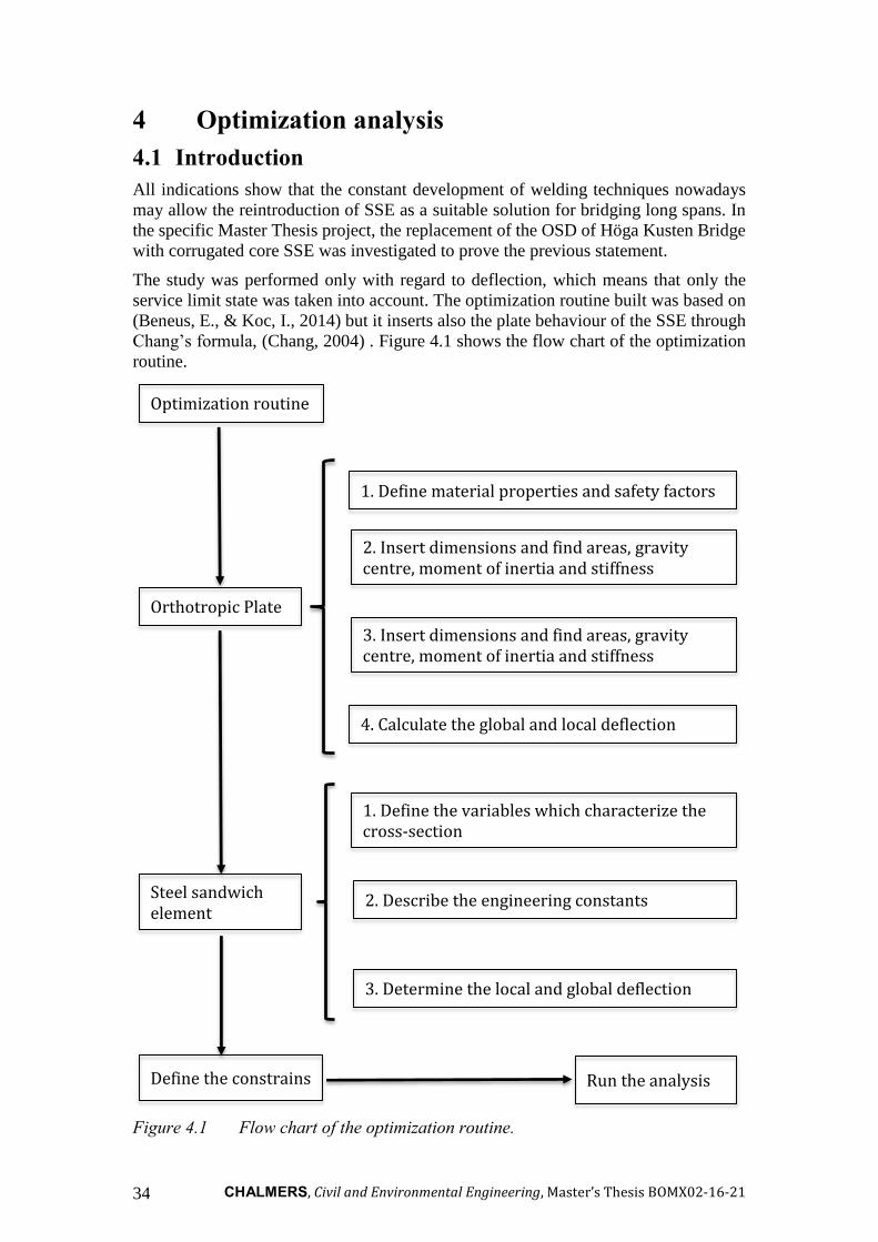
4 Optimization analysis 4.1 Introduction All indications show that the constant development of welding techniques nowadays

may allow the reintroduction of SSE as a suitable solution for bridging long spans. In

the specific Master Thesis project, the replacement of the OSD of Höga Kusten Bridge

with corrugated core SSE was investigated to prove the previous statement.

The study was performed only with regard to deflection, which means that only the

service limit state was taken into account. The optimization routine built was based on

(Beneus, E., & Koc, I., 2014) but it inserts also the plate behaviour of the SSE through

Chang’s formula, (Chang, 2004) . Figure 4.1 shows the flow chart of the optimization

routine.

Figure 4.1 Flow chart of the optimization routine.

Optimization routine

Orthotropic Plate

1. Define material properties and safety factors

2. Insert dimensions and find areas, gravity centre, moment of inertia and stiffness

Steel sandwich element

2. Describe the engineering constants

4. Calculate the global and local deflection

1. Define the variables which characterize the cross-section

3. Insert dimensions and find areas, gravity centre, moment of inertia and stiffness

3. Determine the local and global deflection

Define the constrains Run the analysis


The rigidity and behaviour of the new SSE are affected by the geometry of the section.

The geometry of the section can be defined by 6 parameters, which from this point on

will be referred as the independent variables. For the needs of this specific Master thesis

project, these variables set to be the following, see Figure 4.1:

Figure 4.2 Typical section of V-type corrugated SSE.

the height of the core, hc.ssp

the thickness of the top plate, tf.top

the thickness of the bottom plate, tf.bot

the thickness of the corrugated core, tc.ssp

the angle of the core stiffeners with the horizontal axis, αssp

the horizontal part of the core between two stiffeners, fssp

All the parameters of the algorithm have been defined in relation to the independent

variables of the SSE. Thus, setting values for the independent variables results in a fully

defined SSE section; all the dimensions as well as all the stiffness parameters according

to (Libove, C., & Hubka, R. E., 1951).

The optimization analysis aims at producing sections which will be optimized for a

series of different cases. This was performed through a numerical method suitable to

solve constraint non-linear optimization problems. This iterative method allows a

property of SSE to be maximized or minimized. To execute this numerical approach,

the build-in solver of the calculation program Mathcad used.

In order to obtain the desired results, a number of constraints were set. These constraints

were the conditions which must be valid to create an appropriate final section. The

constraints in all of the analyses, as well as the corresponding input in the routine, are

shown in Table 4.1. The motives behind the selection of these constraints are analysed

in detail in chapter 4.2.

Table 4.1 Constraints in the optimization routine.

Constraint Input

The top and bottom plates should be at least in class 3. 𝑡𝑓.𝑡𝑜𝑝, 𝑡𝑓.𝑏𝑜𝑡 ≤ 42휀

The corrugated core should be at least in class 3. 𝑡𝑐.𝑠𝑠𝑝 ≤ 42휀

tf.top

tc.ssp

hc.ssp

tf.bot

ássp

fssp


The global deflection of the SSE in the center of the plate

should be limited to a value smaller than the smallest

dimension divided by 400. 𝑤𝑡𝑜𝑡 ≤

𝐿𝑠𝑠𝑝

400

The local deflection between the transverse beams of the

SSE should be smaller than the length divided by 400. 𝛿𝐼 ≤𝑙𝑠𝑠𝑝

400

The angle of the corrugated core should be ranging

between 40 and 70°. 40° ≤ 𝑎𝑠𝑠𝑝 ≤ 70°

The distance between the inclined stiffeners of the core

should be between 20mm and 40mm. 20 𝑚𝑚 ≤ 𝑓𝑠𝑠𝑝 ≤ 40 𝑚𝑚

These constraints should be fulfilled in all the cases studied. The different scenarios

considered were:

1) Maximization of the moment of inertia in the longitudinal direction (Ix)

2) Minimizing the material used

3) Minimizing the material used, considering an updated main girder configuration

4) Maximizing the length between the transverse stiffeners

In every scenario a specific property is chosen to be optimized. To optimize the value

of a property, the user must enter the corresponding function in the program,

accompanied by the independent variables by which this property is dependent from.

All the independent variables should fluctuate in the margin set by the constraints.

Furthermore, the user must set initial values for the independent variables for the

program to start running. As explained, the optimization routine is a numerical iterative

method. That means that during the execution of the routine, the program sets values

for the independent variables, until the optimum solution is found depending on each

scenario. The tolerance in the program is set equal to 10-6.

4.2 Choice of the constraints The theory behind the calculations of the limiting values of the constraints will be

discussed in the current section. To begin with, all the individual parts of the cross

section in the routine were chosen to be in class 3 or better. That means that their whole

cross-sectional area could be used in the design and be loaded to the yielding point.

According to (EN 1993-1-1., 2005, Table 5.2), for parts subjected to uniform

compression, the maximum value of the width to thickness ratio is 42ε,

where 휀 = √235 𝑓𝑦⁄

Structural steel grade S355 was chosen, with fy = 355MPa, resulting in ε = 0,814.

Therefore, the width to thickness ratios of the several parts of the cross section should

be below 34.2.

Furthermore, the deflection between the diaphragms was set to be smaller or equal than

their distance, which is 4 meters, divided by 400, i.e. 10 millimetres. The deflection in

the routine was calculated for a simply supported plate equally wide to the half of the

total width (9 m) and equally long to the length between the diaphragms (4 m). The

deflection was calculated using double Fourier series, based on the Mindlin–Reissner


plate theory, see (Chang, W.-S., 2004). The distributed load applied consists of the

traffic load for the main and the secondary lanes which is 9 and 2,5 kN/m2 respectively

as well as the asphalt load and the self-weight of the construction. The asphalt load is

1,15 kN/m2 for asphalt 50 mm thick. The self-weight for a section with the same amount

of material as the orthotropic deck of the Höga Kusten bridge is 1,727 kN/m2. In

addition to this, there is also the load from two vehicles. The load according to (EN

1991-2, 2010) is 150 kN per wheel for the main lane and 100 kN per wheel for the

secondary. The distance between the wheels of each truck is 1,2 m in the direction of

the traffic flow and 2 m in the transverse direction. The magnitudes and the positions

of the loads are shown in Figure 4.2. It should be noted that, due to the difficulty to

calculate the deflection for different uniform loads in different lanes, the uniform loads

were transformed in an equivalent uniform load which acts all over the plate. The value

of this load was 4,67 kN/m2.

Figure 4.3 Load magnitudes and positions.

The calculation of the deflection using a simply supported plate does not represent the

reality, since there is also the continuity of the plate over the supports which will result

in a lower deflection value. To find a more accurate deflection between two consecutive

transverse beams including the effect of the continuity, the Finite Element (FE) program

Abaqus/CAE was used. Verification of the FE analysis was made, in order to ensure

that there is correspondence between its results and the analytical solution. The

verification can be found in chapter 5.5.

Another constraint was set due to the local deflection. According to this constraint the

deflection between the core repetitions (δI) should be less than the repetition length (lssp)

divided by 400, see Figure 4.3. The applied load is the wheel load divided by the width

of the wheel increased by 100 mm, see Figure 4.4.

9m

3m 3m 3m

Main Lane

4m

2m

1.2

m

x

y

Secondary

LaneSecondary

Lane

2.5 kN/m² 2.5 kN/m²9 kN/m²

150 kN 100 kN


Figure 4.4 Local deflection of SSE.

Furthermore, the angle of the corrugated core (αssp), was set between 40 and 70 degrees,

while the distance between the inclined stiffeners of the core (fssp) was chosen to be

between 20 and 40 mm.

4.3 The studied scenarios 4.3.1 Maximization of the moment of inertia in the longitudinal

direction Following the same concept as (Beneus & Koc 2014), the initial purpose was to create

a steel sandwich element for the Höga Kusten Bridge, which would have a better

structural behaviour than the existing orthotropic deck. For this purpose, the first use of

the optimization routine was the design of an SSE which could the same amount of

material and at the same time better moment of inertia in the longitudinal direction (x-

direction).

4.3.2 Minimizing the material used From the literature study, it was underlined that the main asset of the SSE is its potential

to behave as a plate and distribute the loads in both directions. Therefore, the total

deflection of the plate was studied rather than the bending stiffness in the strong

direction. This was achieved by adjusting the optimization routine to minimize the

global deflection in the middle of the plate.

To verify the results a plate model was then created in Abaqus/CAE, where a single

layer homogenous core was adopted, as described in (Romanoff & Kujala 2002). The

model was generated as a lamina plate using the engineering constants from the

optimization routine. The point in which the maximum global deflection appeared in

the FEM approach was then compared with the point assumed to deflect more in the

optimization routine; in the specific case the middle of the plate.

Provided that there should exist no point in the plate with higher deflection than the

minimum value of Lssp/400 and Bssp/400, the previous optimization routine was rerun,

searching the deflection in the new spot found and assuming that this point would not

change due to the different cross-section obtained. The reutilization of the routine

provided the right value for the maximum deflection. In the end of the procedure, it had

been verified that the most deflected point stayed immovable.

300 kN/m

a

lssp


However, the results obtained were reflecting the behaviour of a single supported SSE,

which is not the real case in long-span decks. So, the next step was to take into account

the continuity of the plates between the diaphragms that form the bridge deck. In this

occasion the whole deck was modelled in Abaqus/CAE. The deflection of the

equivalent plate was calculated for a continuous plate 9 m wide, which is the half of the

deck width, simply supported every 4 m, which is the distance between the transverse

beams, for a total length of 20 m, which was the distance between the diaphragms in

the Höga Kusten case. By creating the bridge geometry in Abaqus/CAE, with the

corresponding loading, the real global deflection could be extracted.

4.3.3 Minimizing the area by adding a longitudinal stiffener In this case, the above analysis and methodology was implemented with the addition of

a longitudinal stiffener in the middle of the width of the plate. The aim was the creation

of two more square shaped steel sandwich plates that would grant improved structural

behaviour compared with the original rectangular plate of the previous scenario. This

stiffener, which was modelled as a support, resulted in panels 4 m long and 4,5 m wide.

A new equivalent uniformly distributed load was calculated, as only the main vehicle

could fit in the deck lane.

4.3.4 Maximizing the length between the transverse stiffeners The final study that was performed was the investigation of the maximum length that

the SSE could have between two diaphragms. In this case, the routine aimed to optimize

the plate’s length, while the material used on the SSE section was set equal to the OSD.

The purpose of the specific study was to investigate if it is possible to reduce the number

of the transverse beams, and thus, save material. The major advantage of the SSE

compared to the OSD is the fact that it provides much larger stiffness in the y-direction.

Therefore, the increment of its length would be beneficial by enhancing the plate

behaviour of the SSE. Moreover, apart from saving material by decreasing the number

of the transverse stiffeners, the implementation of longer elements would reduce

significantly the production time and cost.

4.4 Finite Element Analysis As mentioned above, in order to take into account the continuity of the plates between

diaphragms, the FEM program Abaqus/CAE was used. The Simplified Finite Element

Approach, as described in (Romanoff & Kujala 2002) was used. The geometry of the

bridge deck between the diaphragms was modelled for all the examined cases.

However, the final steel sandwich sections were not modelled in detail as that could not

give more value to the aim of this Master Thesis project. Instead the elements used were

3D deformable shell elements including shear-induced vertical displacements. The

elastic properties of the material were defined using lamina material model and the

engineer constants for out-of-plane condition were obtained from (Lok & Cheng 2000):

𝐸𝑥 =12∙𝐷𝑥

ℎ3, (4.1)

𝐸𝑦 =12∙𝐷𝑦

ℎ3, (4.2)

𝐺𝑥𝑦 =6∙𝐷𝑥𝑦

ℎ3, (4.3)


𝐺𝑥𝑧 =𝐷𝑄𝑥

𝑘∙ℎ, (4.4)

𝐺𝑦𝑥 =𝐷𝑄𝑦

𝑘∙ℎ, (4.5)

where k is the shear correction factor; chosen equal with 5/6.

Regarding the boundary conditions, the translation in the vertical direction was

prevented on the outer edges of the plate, as well as in the positions of the transverse

stiffeners. In addition to this, the longitudinal movement was also prevented where a

longitudinal stiffener was added in one of the studies.

For the mesh, 4-node elements were used with quad-dominated shape. The approximate

size of the elements was 250 mm.

Finally, the loading was set as pressure for both the uniform distributed load as well as

for the wheel loads. The uniformly distributed load, which included the self-weight, the

traffic and the asphalt loads, was 7,544 kN/m2 in the cases where the area of the section

was equal to the one of the orthotropic section. In the cases where this area is reduced,

this load somewhat smaller. The wheel loads were set as pressure over an area of 500

x 500 mm which was defined by (EN 1991-2, 2010) increased by 100 mm, to account

the height of the asphalt, see Figure 4.4.

Figure 4.5 Distribution of the wheel load in the pavement.

Pavement

400 mm

500 mm45°

50

mm


5 Results In this chapter the results from the different analyses are presented. For detailed

calculations see Appendix A.


Τhe first study has proven that with the specific amount of material given by the cross

section of Höga Kusten deck and all the constraints considered, it was hard to create a

steel sandwich element that could have larger moment of inertia in the direction of the

traffic flow. The reason was that the existing bridge deck consists of quite slender parts

(i.e. the webs are in class 4). On the other hand, the SSE was constrained to achieve

cross-sectional properties of class 3 or lower and thus to provide a structural member

with all the individual parts insensitive to local buckling.

5.2 Study 2 - Minimization of the material used The most important conclusion of this scenario was the proof that studying the steel

sandwich element as a plate did give the opportunity of reducing the area of the cross

section in long span bridges.

The first phase of the analysis was the usage of the routine for the acquisition of an

initial cross-section that could be used for extracting the most deformed point. An FE

model was then created in Abaqus/CAE, as explained in Chapter 4.3.2. The result for

the equivalent plate is illustrated in Figure 5.1.

Table 5.1 Initial cross-section for the formation of the Abaqus/CAE model in Study 2.

Optimization Results

Function Minimize wtot

Global deflection (for i,j=1…1) in the optimization routine

wtot mm 6,72

Height of the core hc.ssp mm 163,0

Thickness of the upper plate tf.top mm 6,5

Thickness of the bottom plate tf.bot mm 5,1

Thickness of the core tc.ssp mm 5,3

Angle of the core assp degrees 64,7

Distance between diagonals f.sp mm 21,6

Engineering Constants

Exb N/mm2 55730

Eyb N/mm2 46170

Gxy.1 N/mm2 16020

Gxz N/mm2 4470

Gyz N/mm2 642,8

To ensure that the deflection values calculated from the hand calculations and

Abaqus/CAE correspond well to each other, there has been a verification which may

be found later in this chapter.


Figure 5.1 Deflection in the middle of the plate for the equivalent plate in Abaqus/CAE. It was observed that the maximum deflection was obtained in a different point and not

in the middle of the plate. That was expected due to the asymmetric traffic loading. The

point of the maximum deflection had coordinates (X, Y) = (2m, 5,4m). The coordinates

of this spot as well as the value of its deflection are shown in the Figures 5.1 and 5.2.

Figure 5.2 Maximum deflection point for the equivalent plate in Abaqus. Having extracted the most the most deflected point, a new cross-section was searched

out with the assistance of the optimization routine, which gave the following results

(Table 5.2).


Table 5.2 Cross-section which includes the correct coordinates for the point with the maximum deflection and has been used in the continuous plates in Study 2.

Optimization

Results


Global deflection (for i,j=1..1) in the

optimization routine wtot mm 6,39






Distance between diagonals fssp mm 21,6


Exb N/mm2 55730

Eyb N/mm2 46170

Gxy.1 N/mm2 16020

Gxz N/mm2 4470

Gyz N/mm2 642,8

Comparison between Huga

Kusten and SSE

Length between transversal beams ΔLssp (L.ssp-L.HK)/L.HK -

Area ΔAssp (A.ssp-A.HK)/A.HK -

Moment of Inertia ΔIx (I.x.ssp-I.x.HK)/I.x.HK -59,2%

ΔIy (I.y.ssp-I.y.HK)/I.y.HK 6,6*104%

Axial Stiffness ΔEx (E.x.ssp-E.x.HK)/E.x.HK -

ΔEy (E.y.ssp-E.y.HK)/E.y.HK -2,850%

Bending Stiffness ΔDx (D.x.ssp-D.x.HK)/D.x.HK -59,2%

ΔDy (D.y.ssp-D.y.HK)/D.y.HK 6,1*104%

Torsional Stiffness ΔDxy (D.xy.ssp-D.xy.HK)/D.xy.HK 897,5%

Transversal Shear Stiffness ΔDQ.x (D.Q.x.ssp-D.Q.x.HK)/D.Q.x.HK 409,705%

The cross-section that was created from the optimization routine was exactly the same

as the previous analysis and that happened due to the fact that in none case the global

deflection was exceeding the allowable limit. However, it was noticed that the

maximum global deflection was smaller than the previous analysis, which happened

because the analysis was run for i and j equal to 1, i.e. no iterations. Therefore an

Abaqus equivalent plate was created again. The Abaqus model gave the below results.


Figure 5.3 Deflection results for the analysis of the cross-section in Table 5.2.

The deflection magnitude obtained from Abaqus was 7,35mm. The difference between

this value and the analytical solution had to do with the number of iterations. For an

increased number of iterations the two solutions converged. The reason why in the

specific study i and j were taken equal to 1 was the fact that for increased values of

them the routine was becoming rather time consuming.

As described in Chapter 4.3.2, the comparison between the two decks in that point was

not correct as the global deflection for the OSD was measured for a continuous beam

while in the SSE was calculated for a simple supported plate. The design of a new FEM

model with 5 continuous plates between the diaphragms provided the results illustrated

of the Figure 5.4.

Figure 5.4 Results for deflection using the continuity of the plate in Table 5.2.

With the continuity condition, the deflection value was 3,96mm. Therefore, it was

possible to construct an SSE that would have the same deflection with the orthotropic

section, but less material per unit width. Another optimization routine was run in order

to minimize the area of the steel sandwich element. The target of the investigation was

to create a lighter element that would have the same maximum deflection with the

orthotropic deck. However, to move from the simply supported plate, which was used

in the optimization, to the continuous one, which was the case in reality, the ratio of the

deflection for the two cases was used. Thus, the allowable deflection in the optimization

was multiplied by 7,35mm/3,96mm=1,86. The results, for minimizing the total area of

the steel sandwich element, were the following:


Table 5.3 Cross-section after inserting the deflection ratio due to the continuous plates in Study 2.

Optimization

Results

Function Minimize Assp

Global deflection (for i,j=1…1) in the









Exb N/mm2 56040

Eyb N/mm2 46660

Gxy.1 N/mm2 16010

Gxz N/mm2 4353

Gyz N/mm2 451,7

Comparison

between Huga

Kusten and SSE


Area ΔAssp (A.ssp-A.HK)/A.HK -13,7%



Axial Stiffness ΔEx (E.x.ssp-E.x.HK)/E.x.HK -13,653%






ΔDQ.y (D.Q.y.ssp-D.Q.y.HK)/D.Q.y.HK -

The Abaqus equivalent plate from the above results had the below behaviour (Figure

5.5).

Figure 5.5 Deflection results for the cross-section presented in Table 5.3.


Figure 5.6 Global deflection for the SSE presented in Table 5.3 including the continuity of the plate.

The ratio between the simply supported plate and the continuous one was

11,38mm/6,04mm=1,88. This value was very similar to the obtained ratio from the

previous analysis. Thus, it was assumed that the ratio remained almost the same

,independent of the different properties of the lamina plate and so it was acceptable to

approve the final results.

However, the assumption that the new SSE would end up with an equal or smaller

deflection than the OSD was not valid in this case, since the maximum deflection for

the SSE was 6,04 mm. For that reason, a tighter constraint was set for the area per unit

width and the optimization routine for minimizing the global deflection was executed

again. After an iterative procedure, the below results (Table 5.4) were extracted by

using the 90,55% of the initial area. The SSE was having a global deflection of 8,51mm

and 5,26mm for the simply supported and the continuous plate respectively.


Table 5.4 Final cross-section after allowing a tighter constrain for the area per unit width in Study 2.


Optimization

Results


wtot mm 8,51








Exb N/mm2 55904

Eyb N/mm2 46454

Gxy.1 N/mm2 15998

Gxz N/mm2 4395

Gyz N/mm2 503,4

Comparison

between Huga

Kusten and SSE




ΔIy (I.y.ssp-I.y.HK)/I.y.HK -9,5%








Global deflection for continuous plates (Abaqus) wtot mm 5,26

Final equivalent distributed load qeq kPa 7,380

Figure 5.7 Deflection of the SSE cross-section of Table 5.4 including the continuity of the plate.


The same principle was also used in the optimization routine for minimizing the area

of the SSE by setting a looser constraint for the deflection. The results were exactly the

same with the above cross-section showing that the two solutions were converging to

an optimum one. The Abaqus simulation for the following case is not illustrated as it is

exactly the same as in the Figure 5.7. However, the table with the results is shown

below.

Table 5.5 Final cross-section after allowing a looser constrain for the deflection in Study 2.

Optimization

Results



wtot mm 8,515

Height of the core hc.ssph.core mm 147,6







Exb N/mm2 55940

Eyb N/mm2 46498

Gxy.1 N/mm2 16017

Gxz N/mm2 4391

Gyz N/mm2 505

Comparison

between Huga

Kusten and SSE












Global deflection for continuous plates (Abaqus) wtot mm 5,26

Global deflection for simply supported plate (Abaqus) wtot mm


Summing up, both analyses converge to an SSE that reduces the material used by 9,45%

compared with the existing bridge deck. That means that it is possible to save 2120

mm2 of material per unit width (m). Regarding the total length of the bridge this is

translated in tons of material saved. The cross-section of the new steel sandwich

element is illustrated below.


Figure 5.8 Final cross-section of the new steel sandwich element that minimizes the material used.

5.3 Study 3 - Minimizing the material used by adding a longitudinal stiffener

For the third scenario a longitudinal stiffener has been added under the steel sandwich

element as described in chapter 4.3.3. The methodology followed was exactly the same

as the previous study. The results are shown in the table and the figures below. The

maximum deflection turned up in the middle of the plate, while the ratio of the simply

supported plate to the continuous one was calculated equal with

4,27mm/2,40mm=1,779.


Table 5.6 Initial cross-section obtained in Study 3.

Optimization

Results



wtot mm 6,39








Exb N/mm2 55730

Eyb N/mm2 46170

Gxy.1 N/mm2 16020

Gxz N/mm2 4470

Gyz N/mm2 642,8

Comparison

between Huga

Kusten and SSE












Global deflection for continuous plates wtot mm 2,40

Global deflection for simply supported plate wtot mm 4,27


Figure 5.9 Deflection results for a simple supported SSE with the properties described in Table 5.6.


Figure 5.10 Deflection results for the continuous SS plate described in Table 5.6.

By adopting the ratio mentioned above and aiming for the same deflection as the

existing orthotropic deck, which was 5,26mm, the optimization routine for minimizing

the area of the material for the SSE was used.

Table 5.7 Final cross-section in Study 3.


Function Minimize Atot

Global deflection (for i,j=1..1) in the









Exb N/mm2 59095

Eyb N/mm2 50292

Gxy.1 N/mm2 17437

Gxz N/mm2 3972

Gyz N/mm2 471,8

Comparison

between Huga

Kusten and SSE



Moment of Inertia ΔIx (I.x.ssp-I.x.HK)/I.x.HK -82,0 %

ΔIy (I.y.ssp-I.y.HK)/I.y.HK 3*104%










Figure 5.8 Final deflection results for the continuous SSE described in Table 5.7.

The final deflection for the continuous plate was 5,23mm, which is almost the same as

the deflection of the orthotropic section. Therefore, the SSE with the above

characteristics was acceptable. With the specific cross-section and configuration, about

23,7% of material could be saved. That means that a total of 5314 mm2 of material per

unit width can be saved. Of course this should be decreased by the area of the

longitudinal stiffeners. To make a rough estimation, a longitudinal stiffener with profile

IPE 360 was chosen as longitudinal stiffener. For details see Appendix A. This section

has an area of 7270 mm2. The total amount of material saved for the half of the width

is 5314*9 = 47826 mm2, and subtracting the area of the stiffener it end ups to 40556

mm2 of material saved. This equals to 4506 mm2 material per unit width or 20,1% saved

material.

The final cross-section of the SSE for the 4m×4,5m plate is shown in Figure 5.12.

Figure 5.12 Cross-section of the new steel sandwich element.


5.4 Study 4 - Maximizing the length between the transverse stiffeners

The final study included the maximization of both the plate deflection and the length

of the SSE by using again the constraints mentioned in chapters 4.1 and 4.2. The

continuity of the plates was inserted again in the study with the help of Abaqus/CAE.

The results from the analysis are shown below in the Table 5.8.

Table 5.8 Initial cross-section obtained in Study 4.


Function Max wtot and Lssp

Length between transversal beams Lssp m 4,64





Angle of the core assp degrees 64


Engineering constants

Exb N/mm2 52251

Eyb N/mm2 43718

Gxy.1 N/mm2 15456

Gxz N/mm2 3984

Gyz N/mm2 604

Comparison

between Huga

Kusten and SSE

Length between transversal beams ΔLssp (L.ssp-L.HK)/L.HK 16,0%











Limit for the total deflection L/400 mm 11,6


From the first analysis, it was acquired an increase in the length equal to 16%. However,

the global deflection of the plate was still much smaller than the allowed limit. This

happened because the optimization routine could not take into account the continuity

of the plates, as mentioned before. So, a looser constraint for the global deflection was

decided. Furthermore, it was observed that the maximum deflection was very close to

the centre of the plate although the loading was asymmetric. The reason was that the

SSE was behaving more like a plate compared with the previous studies, distributing

the loads in two directions.


By setting different constraints for the simply supported case, an iterative analysis was

used to get the global deflection of the continuous sandwich elements closer to the

allowed limit. The final iteration gave the results presented in Table 5.9.

Table 5.9 Final cross-section from Study 4. Function Max wtot and,Lssp

Optimization

Results

Length between transversal beams Lssp m 7,38





Angle of the core assp degrees 63


Comparison

between Huga

Kusten and SSE

Length between transversal beams ΔLssp (L.ssp-L.HK)/L.HK 92,9%





ΔEy (E.y.ssp-E.y.HK)/E.y.HK 0,9%






Limit for the total deflection L/400 mm 18,46


Figure 5.9 Final deflection results for the continuous SSE described in Table 5.9.

The conclusions demonstrate that the length of the bridge deck between two transversal

stiffeners could be increased up to 92,9% by using steel sandwich elements for the case

of the Höga Kusten bridge.

5.5 Verification of the deflection To confirm the correspondence between the analytical calculation of deflection and the

results from Abaqus/CAE, a comparison between their results was made. This was

performed for a simply supported plate. For the calculation of the deflection with the

analytical model the optimized section for each case is used, for 21 iterations.


Table 5.10 Difference between hand calculations and Abaqus/CAE for a bigger number of iterations.

Deflection between transverse beams

(mm)

Plate dimensions (m)

Analysis Deflection Point

X, Y Hand calculations Abaqus Difference

4x9

Part 1 2 , 4.5 6,57 6,71 2,13%

Part 2 2 , 5.4 7,17 7,35 2,51%

Part 3 2 , 5.4 11,00 11,24 2,21%

Part 4 2 , 5.4 9,56 9,80 2,47%

Part 5 2 , 5.4 9,56 9,80 2,47%


5.6 Moment and axial capacity As mentioned, the studies performed in this work compared only by the deflection

between the conventional orthotropic deck of Höga Kusten bridge and the potential

steel sandwich elements in the SLS. However, any changes in the configuration of the

cross-section of the bridge deck has impact on the design moment and axial load

carrying capacity. Therefore, these parameters in relation with the corresponding values

of the initial deck were studied. The results are summed up in the Tables 5.11 and 5.12

below, while further calculations could be found in the Appendix B. The calculations

have been executed according to (EN 1993-1-1, 2005).

Table 5.11 Moment and axial capacity of the original orthotropic deck as well as the SSE created in the different studies.

Studies Parameter Units Value

Orthotropic Deck of Höga

Kusten Bridge

Reduction factor xρ.c for column-like buckling - 0.862

Reduction factor xρ.pl for plate-like buckling - 1

Total reduction factor xρ - 0.886

Moment capacity kN×m/m 444.129

Axial capacity kN/m 6.718×103

Study 2 - Minimizing the

material used


Reduction factor xρ.pl for plate-like buckling - 0.996





material used by adding a

longitudinal stiffener


Reduction factor xρ.pl for plate-like buckling - 1




Study 4 - Maximizing the

length between the

transverse stiffeners


Reduction factor xρ.pl for plate-like buckling - 0.872





Table 5.12 Comparison between the moment and axial carrying capacity between the initial orthotropic bridge deck and the SSEs.

Comparison of the moment and axial capacities of the different studies with the initial orthotropic bridge deck

Studies Parameter compared Formula Value


material used

Moment capacity MRd (MRd.ssp1 - MRd) / MRd - 16.888%

Axial capacity NRd (NRd.ssp1 - NRd) / NRd - 8.564%

Study 3 – Minimizing the



Moment capacity MRd (MRd.ssp2 - MRd) / MRd -40.635%


Study 4 – Maximizing the

length between the transverse

stiffeners

Moment capacity MRd (MRd.ssp3 - MRd) / MRd 1.479%


However, the carrying capacity of the newly generated SSEs would only have meaning

if it was directly connected to the loading of the deck. And that is due to the fact that

changes in the dimensions of the plates in the different studies would affect the acting

moment on the bridge deck. Therefore, in every study performed the acting moment

has been extracted in order to calculate the utilization factor with the assistance of

Abaqus/CAE. Figures 5.14-16 and table 5.13 show the values of the moment in every

scenario, while table 5.14 demonstrate the respective utilization factors. Furthermore,

the acting moment of every optimized model was compared to their bending capacity,

see tables 5.13 and 5.14.

Table 5.13 Acting moment in the different scenarios.

Studies Parameter compared Notation Value (kNm/m)


material used Acting moment MEd.ssp1 MEd.ssp1 76.20




Acting moment MEd.ssp2 MEd.ssp2 50.20



stiffeners

Acting moment MEd.ssp3 MEd.ssp3 139.40


Figure 5.10 Acting moment (76.20 kNm/m) in Study 2.




Table 5.144 Utilization factor for the moment capacity in the different scenarios. Calculation of the utilization factors for the moment capacities of the different studies with the initial

orthotropic bridge deck

Studies Parameter compared Formula Value


material used

Utilization factor for the

moment

capacity uM.ssp1

MEd.ssp1 / MRd.ssp1 0.206





moment

capacity uM.ssp2




stiffeners


moment

capacity uM.ssp3



6 Discussion The purpose of this Master thesis project was the investigation of how effective the

steel sandwich elements may be, when they were utilized as part of the stiffening girder

of a suspension bridge. The study was performed in the serviceability limit state. The

results showed that in almost all the scenarios studied, steel sandwich decks may reduce

significantly the amount of steel used for the bridging of long spans compared with

convectional solutions. In the following sub-chapters there is a discussion about the

results that the different optimization routines produced.


In the first case, the optimization aimed to maximize the moment of inertia in the

longitudinal direction. However, the results showed a significant lower moment of

inertia compared to the orthotropic steel deck. Taking into consideration the fact that

the superior property of the orthotropic deck is the moment of inertia in the longitudinal

direction and that the original OSD was quite slender - web in class 4 -, the result

seemed to be reasonable.

6.2 Study 2 - Minimization of the material used The second case which was examined was an attempt to minimize the material used in

the cross-section by restraining the deflection of the upper flange of the box girder

between the transverse beams in the optimization routine. In this scenario the fact that

in the first attempt the deflection between transverse beams was smaller when using

sandwich elements than with the OSD led to a sub-study to investigate the possible

reduction of the area per unit width, if the original section was replaced by an SSE and

the deflection remained constant. The 10% in material reduction was absolutely an

amount that could not be unnoticed especially in so large scale constructions like cable

bridges. The main reason for this result was the two-way plate behaviour of the SSE

compared with the OSD. This could also conclude, apart from the main deck, to a chain

material deduction in almost all the parts of the bridge like the hangers, the main cables

and the pylons, as the self-weight of the bridge deck would be decreased.

6.3 Study 3 - Minimizing the material used by adding a longitudinal stiffener

Another study was conducted to investigate the behaviour of the sandwich section when

the geometry of the bridge tended to be more square-shaped. In this scenario it was

assumed that in the half of the bridge deck a longitudinal stiffener was added, resulting

in smaller almost square plates. The deflection between the transverse beams was again

equal to the one of the orthotropic section, whilst the area per unit width was reduced

as much as possible. The results here was a reduction of the area of about 23%, and

with a rough calculation for the dimensions of the longitudinal stiffener it was

advantageous compared to the first investigation. However, the reader should keep in

mind that this solution may increase the cost, as well as the production time, due to the

increased and more complicated welding.


6.4 Study 4 - Maximizing the length between the transverse stiffeners

In this case the aim was to increase the distance between the transverse beams, in order

to be able to decrease their number and save material that way. This was done by

maximizing the allowable deflection between the transverse beams up to the limit value,

which is the length divided by 400. The results showed that using sandwich elements

could result in a significant increment of the length between transverse beams.

Particularly the length could be increased by 92.9%, which resulted to plates 7.38 m

long and 9 m wide in the Höga Kusten bridge case. The logic behind that was that the

bridge deck was allowed to maximize itself its length keeping the width constant and

thus take the most optimum shape depending on its stiffness constants.


7 Conclusions In this master thesis project, the possibility of replacing conventional orthotropic steel

decks with a steel sandwich bridge deck was investigated with respect to serviceability

limit state. The results of the different studies conducted is encouraging and allow the

further research of the topic.

In general, the concluding remarks from this project could be summed up the following:

The utilization of SSE bridge decks could result in smaller deflections between

the transverse beams compared to conventional orthotropic decks.

With equal bending stiffness, the SSE utilizes less material compared to the

convectional solutions. Width to length aspect ratios close to 7 was shown to

increase the effectiveness of the SSE bridge deck.

The distance between transverse beams could be increased when using SSE

compared to the convectional solutions. Therefore, material could be saved

from the reduction of the number of the transverse stiffeners.

As far as the bending moment capacity of the newly created SSEs is concerned,

it was proven that the SSEs had quite lower bending stiffness compared with

the original OSD due to their smaller total height. However, the Abaqus/CAE

analysis had proven also that the bending moment acting on the SSEs would

have also a lower value as their plate behaviour distributed the stresses with a

more efficient two-way action.


8 References

Allen, H. G. (1969): Analysis and Design of Structural Sandwich Panels. Analysis and Design of Structural Sandwich Panels. Pergamon Press.

http://doi.org/10.1016/B978-0-08-012870-2.50011-0

Alwan, U., & Järve, D. (2012): New Concept for Industrial Bridge Construction. M.Sc.

Thesis, Department of Structural Engineering, Chalmers University of

Technology, Publication no. 2012:110, Göteborg, Sweden.

Banck, F., & Almberg, O. R. (2014). Application of CFRP Cables in Super Long Span Cable Supported Bridges. M.Sc. Thesis, Department of Structural Engineering,

Chalmers University of Technology, Publication no. 2014:95, Göteborg, Sweden.

Beneus, E., & Koc, I. (2014). Innovative road bridges with steel sandwich decks. M.Sc.

Thesis, Department of Structural Engineering, Chalmers University of

Technology, Publication no. 2014:138, Göteborg, Sweden.

Billington, C. J., Chapman, J. C., Dowling, P. J., & Lim, P. T. K. (1971). The structural behaviour of steel and concrete box girder bridges, 49(3), 111–120.

Chang, W. S., Ventsel, E., Krauthammer, T., & John, J. (2004). Bending behavior of

corrugated-core sandwich plates. Composite Structures, 70(1), 81–89.

http://doi.org/10.1016/j.compstruct.2004.08.014

Chang, W.-S. (2004). Elasto-Plastic Analysis of Corrugated Sandwich Steel Panels.

The Pennsylvania State University.

Chatterjee, S. (2003). The Design of Modern Steel Bridges. Blackweel Science (Second

Edi). Blackweel Science. http://doi.org/10.1002/9780470774373

Chen, W.-F., & Duan, L. (2014). Bridge Engineering Handbook (2nd ed.).

Chen, Y. S., & Yen, B. T. (n.d.). Analysis of Composite Box Girders (Vol. 12). Fritz

Engineering Laboratory.

Djubek, J., Kondar, R., & Skaloud, M. (1983). Limit State of the Plate Elements of

Steel Structures (pp. 220–255).

EN 1993-2:2006. (2011). Eurocode 3: Design of steel structures - Part 2: Steel bridges.

EN1991-2. (2010). Eurocode 1: Actions on structures - Part 2: Traffic loads on bridges.

EN 1993-1-1. (2005). Eurocode 3: Design of steel structures - Part 1-1: General rules and rules for buildings.


Feldmann, M., Sedlacek, G., & Geßler, a. (2007). A system of steel-elastomer sandwich

plates for strengthening orthotropic bridge decks. Mechanics of Composite Materials, 43(2), 183–190. http://doi.org/10.1007/s11029-007-0018-y

Finley, J. (1810). The Portfolio - The Chain Bridge.

Gimsing, N., & Georgakis, C. (2012). Cable Supported Bridges: Concept and Design.

Wiley (Vol. 27). Wiley. http://doi.org/10.1016/j.jfluidstructs.2011.04.006

Guohao, L. (1987). Analysis of Box Girder and Truss Bridges. China Academic

Pubilshers. Retrieved from http://gjgcb.sirt.edu.cn/UploadFile/ZL/F1/Analysis of

Box Girder and Truss Bridges.pdf

Hambly, E. C. (1991). Bridge Deck Behaviour (2nd ed.). E & FN SPON.

Helwig, T., Yura, J., Herman, R., Williamson, E., & Li, D. (2007). Design Guidelines For Steel Trapezoidal Box Girder Systems (Vol. 7).

Institute for Steel Development & Growth. (1999). Beams subjected to torsion and bending.

Kennedy, D. J. L., Dorton, R. A., & Alexander, S. D. B. (2002). The Sandwich Plate System For Bridge Decks.

Kolsters, H., & Wennhage, P. (2009). Optimisation of laser-welded sandwich panels

with multiple design constraints. Marine Structures, 22(2), 154–171.

http://doi.org/10.1016/j.marstruc.2008.09.002

Kujala, P., & Klanac, A. (2005). Steel sandwich panels in marine applications.

Brodogradnja, 56, 305–314.

Lebet, J.-P., & Hirt, M. (2013). Steel Bridges Conceptual and Structural Design of Steel and Steel-Concrete Composite Bridges Title. EPFL Press.

Libove, C., & Hubka, R. E. (1951). Elastic Constants for Corrugated-Core Sandwich

Plates. NACA TECHNICAL NOTE 2289.

Lok, T.-S., & Cheng, Q.-H. (2000). Analysis of Sandwich Panel as a 2-D Orthotropic

Thick Plate Continuum. International Offshore and Polar Engineering Conference, IV, 110–115.

US Department of Transportation, U. S. D. (2012). Steel Bridge Design Handbook

Structural Behavior of Steel.

Peter, W. (1987). The significance of warping torsion in the design of straight concrete

box-girder bridges.

Peters, T. F. (1980). The first wire suspension bridge : Geneva 1823, 7.


Roman, W. (1963). Design Manual for Orthotropic Steel Plate Deck Bridges. American

Institute of Steel Construction.

Romanoff, J. (2007). Bending Response of Laser-Welded Web-Core Sandwich Plates.

Helsinki University of Technology.

http://doi.org/10.1016/j.compstruct.2006.08.021

Romanoff, K., & Kujala, P. (2002). Formulation for the strength analysis of all steel

sandwich panels.

Ronald, F., Manzon, L., Kujala, P., Brede, M., & Weitzenböck, J. (2004). Advanced

joining techniques in European shipbuilding. Journal of Ship Production, 20(3),

200–210.

Sir William Fairbairn. (1849). An Account of the Construction of the Britannia and Conway Tubular Bridges, with a Complete History of their Progress. John Weale.

Timoshenko, S., & Woinowsky-Krieger, S. (1989). Theory of Plates and Shells

(Second Edi). McGraw-Hill Book Company.

Troitsky, M. S. (1968). Orthotropic Bridges : Theory and Design.

US Department of Transportation. (2012a). Manual for Design, Construction and

Maintenance of Orthotropic Steel Deck Bridges.

US Department of Transportation. (2012b). Steel Bridge Design Handbook Structural

Behavior of Steel.

Wai-Fah, C., & Lian, D. (2014). Bridge Engineering Handbook, Construction and Maintenance. CRC Press (Second Edi). CRC Press.

Waldron, P. (1988). The significance of warping torsion in the design of straight

concrete box girder bridges. Canadian Journal of Civil Engineering, 15(5).

Xanthakos, P. P. (1993). Theory and Design of Bridges (1st ed.). John Willey & Sons.

Xu, Y. L., & Xia, Y. (2011). Structural Health Monitoring of Long-Span Suspension Bridges.

Yilmaz, C., & Wasti, S. T. (1984). Analysis and Design of Bridges. NATO ASI Series.

CHALMERS, Civil and Environmental Engineering, Master’s Thesis BOMX02-16-21

9 Appendix A

Properties

Ma

teri

al P

rop

ert

ies

ν0

.3:=

Po

isso

n's

ra

tio

ρS

35

5N

78

50

kg

m3

:=

De

nsity o

f ste

el

ES

35

5N

21

0G

Pa

:=

Mo

du

lus o

f e

lasticity

Gc

ES

35

5N

21

ν+

()

⋅

80

.76

9G

Pa

⋅=

:=

Sh

ea

r m

od

ulu

s o

f e

lasticity

f y3

55

MP

a:=

Yie

ldin

g s

tre

ng

th

ε2

35

MP

a

f y

0.8

14

=:=

γM

01

:=

γM

11

:=

Sa

fety

fa

cto

rs

t cover

50

mm

:=

Th

ickn

ess o

f th

e a

sp

ha

lt c

ove

r

a d2

3kN

m3

:=

Asp

ha

lt d

en

sity,

acco

rdin

g w

ith

Tra

ffik

ve

rke

t_B

ro_

20

11

, p

g. 4

5

Properties

Höga K

ust

en B

ridge -

Dim

ensi

ons

Hö

ga

Ku

ste

n B

rid

ge

Pa

ram

ete

rs n

ee

d to

be

in

se

rte

d -

All th

e d

ime

nsio

ns a

re m

ea

su

red

fro

m th

e c

en

tre

lin

es (

wh

en

th

is d

oe

s n

ot h

ap

pe

n it is

cle

arl

y s

tate

d)

Wh

ole

bri

dg

e

l lon

g.s

tif

4m

:=

Le

ng

th o

f lo

ng

itu

din

al stiff

en

ers

be

twe

en

ve

rtic

al stiff

en

ers

hb

ox

3.7

82

m:=

He

igh

t o

f th

e b

ox g

ird

er

cro

ss s

ectio

n

To

p f

lan

ge

αH

K.f

.top

atan

2.5

10

0

1

.43

2d

eg⋅

=:=

An

gle

fo

r th

e s

lop

e o

f th

e to

p f

lan

ge

t HK

.f.t

op

12

mm

:=

Pla

te th

ickn

ess in

to

p f

lan

ge

l HK

.f.t

op

.hor

18

.4m

:=

Ho

rizo

nta

l le

ng

th o

f th

e to

p f

lan

ge

bH

K.f

.top

60

0m

m:=

Dis

tan

ce

be

twe

en

to

p r

ibs

yH

K.f

.top

3.8

97

m:=

Me

an

dis

tan

ce

be

twe

en

th

e in

clin

ed

to

p a

nd

th

e h

ori

zo

nta

l b

otto

m f

lan

ge

Wh

ole

bo

x-g

ird

er

cro

ss-s

ectio

n

Cro

ss-s

ectio

n o

f th

e to

p r

ibs

To

p r

ibs

t HK

.rib

.top

8m

m:=

Th

ickn

ess o

f th

e to

p r

ibs

l HK

.rib

.top

.f.t

op

30

6.2

mm

:=

Dis

tan

ce

be

twe

en

rib

we

bs a

t th

e to

p

l HK

.rib

.top

.f.b

ot

15

6.3

mm

:=

Dis

tan

ce

be

twe

en

rib

we

bs a

t th

e b

otto

m

hH

K.r

ib.t

op

30

4m

m:=

Ve

rtic

al h

eig

ht o

f th

e r

ibs

nH

K.r

ib.t

op

30

:=

Nu

mb

er

of

top

rib

s

yH

K.n

.rib

.top

3.7

17

7m

:=

To

p w

eb

s

t HK

.web

.top

12

mm

:=

Pla

te th

ickn

ess o

f th

e to

p w

eb

s

l HK

.web

.top

.hor

1.8

mt H

K.w

eb.t

op

2+

1.8

06

m=

:=

Ho

rizo

nta

l le

ng

th o

f th

e to

p w

eb

s

hH

K.w

eb.t

op

1.5

2m

t HK

.f.b

ot

2+

1.5

26

m=

:=

Ve

rtic

al le

ng

th o

f th

e to

p w

eb

s

yH

K.w

eb.t

op

3.0

19

m:=

Me

an

dis

tan

ce

be

twe

en

th

e in

clin

ed

to

p r

ibs a

nd

th

e h

ori

zo

nta

l b

otto

m f

lan

ge

Sid

e s

tiff

en

ers

nH

K.s

id.s

tif

8:=

Nu

mb

er

of

sid

e s

tiff

en

ers

AH

K.s

id.s

tif

0.0

02

4m

2:=

Are

a o

f e

ach

sid

e s

tiff

en

er

yH

K.s

id.s

tif

3.0

91

3m

:=

Me

an

dis

tan

ce

be

twe

en

th

e in

clin

ed

sid

e s

tiff

en

ers

an

d th

e h

ori

zo

nta

l b

otto

m f

lan

ge

Sid

e s

tiff

en

ing

pla

te

Th

ickn

ess o

f sid

e p

late

t HK

.sid

.pl

12

mm

:=

l HK

.sid

.pl

46

8.4

mm

:=

Le

ng

th o

f sid

e p

late

yH

K.s

id.p

l2

.34

61

m:=

Dis

tan

ce

be

twe

en

th

e s

ide

pla

tes a

nd

th

e h

ori

zo

nta

l b

otto

m f

lan

ge

We

bs o

f th

e b

ox-g

ird

er

cro

ss-s

ectio

n

Inclin

ed

bo

tto

m w

eb

s

t HK

.web

.bot.

in1

2m

m:=

Th

ickn

ess o

f th

e in

clin

ed

bo

tto

m p

late

s in

clu

din

g th

e w

eb

s

l HK

.web

.bot.

hor.

in6

mt H

K.w

eb.b

ot.

in

2+

6.0

06

m=

:=

Ho

rizo

nta

l le

ng

th o

f th

e in

clin

ed

bo

tto

m p

late

s in

clu

din

g th

e w

eb

s

hH

K.w

eb.b

ot.

in2

25

0m

mt H

K.f

.bot

2+

2.2

56

m=

:=

Ve

rtic

al le

ng

th o

f th

e in

clin

ed

bo

tto

m p

late

s in

clu

din

g th

e w

eb

s

yH

K.w

eb.b

ot.

in1

.12

8m

:=

Me

an

dis

tan

ce

be

twe

en

th

e in

clin

ed

bo

tto

m p

late

s a

nd

th

e h

ori

zo

nta

l b

otto

m f

lan

ge

Cro

ss-s

ectio

n o

f th

e b

otto

m r

ibs

Bo

tto

m f

lan

ge

t HK

.f.b

ot

12

mm

≡P

late

th

ickn

ess o

f th

e b

otto

m f

lan

ge

l HK

.f.b

ot

10

m:=

Ho

rizo

nta

l le

ng

th o

f th

e b

otto

m f

lan

ge

Bo

tto

m r

ibs

t HK

.rib

.bot

8m

m:=

Th

ickn

ess o

f th

e b

otto

m r

ibs

l HK

.rib

.bot.

f.to

p1

74

.3m

m:=

Dis

tan

ce

be

twe

en

th

e r

ib w

eb

s a

t th

e to

p

l HK

.rib

.bot.

f.b

ot

50

7.4

mm

:=

Dis

tan

ce

be

twe

en

rib

we

bs a

t th

e b

otto

m

hH

K.r

ib.b

ot

25

4m

m:=

Ve

rtic

al h

eig

ht o

f th

e r

ibs

nH

K.r

ib.b

ot.

in1

0:=

Nu

mb

er

of

inclin

ed

bo

tto

m r

ibs

bH

K.f

.bot

10

75

mm

:=

Dis

tan

ce

be

twe

en

bo

tto

m r

ibs

yH

K.n

.rib

.bot.

in1

.07

69

m:=

Me

an

dis

tan

ce

be

twe

en

th

e in

clin

ed

bo

tto

m r

ibs a

nd

th

e h

ori

zo

nta

l b

otto

m f

lan

ge

nH

K.r

ib.b

ot

9:=

Nu

mb

er

of

ho

rizo

nta

l b

otto

m r

ibs

yH

K.n

.rib

.bot

0.1

55

m:=

Dis

tan

ce

be

twe

en

th

e h

ori

zo

nta

l b

otto

m r

ibs a

nd

th

e h

ori

zo

nta

l b

otto

m f

lan

ge

Pa

ram

ete

rs e

xtr

acte

d b

y th

em

se

lve

s

To

p f

lan

ge

l HK

.f.t

op

2

l HK

.f.t

op

.ho

r

2

cosα

HK

.f.t

op

()

1

8.4

06

m=

:=

Inclin

ed

le

ng

th o

f th

e c

om

pre

ssiv

e f

lan

ge

l HK

.f.t

op

.en

d

l HK

.f.t

op

nH

K.r

ib.t

op

bH

K.f

.top

⋅−

()

2:=

l HK

.f.t

op

.en

d0

.20

3m

=In

clin

ed

le

ng

th o

f th

e e

nd

pa

rts in

th

e to

p f

lan

ge

s

To

p r

ibs

αH

K.r

ib.t

op

atan

hH

K.r

ib.t

op

l HK

.rib

.top

.f.t

op

l HK

.rib

.top

.f.b

ot

− 2

:=

αH

K.r

ib.t

op

76

.15

deg

⋅=

An

gle

of

the

in

clin

ed

we

bs o

f th

e to

p r

ibs

l HK

.rib

.top

.web

hH

K.r

ib.t

op

sinα

HK

.rib

.top

()

0.3

13

m=

:=

Inclin

ed

le

ng

th o

f th

e to

p r

ib w

eb

s

To

p w

eb

s

αH

K.w

eb.t

op

atan

hH

K.w

eb.t

op

l HK

.web

.top

.hor

4

0.1

97

deg

⋅=

:=

An

gle

of

the

to

p in

clin

ed

we

bs o

f th

e c

ross s

ectio

n

l HK

.web

.top

hH

K.w

eb.t

op

sinα

HK

.web

.top

()

2.3

64

m=

:=

Inclin

ed

le

ng

th o

f th

e to

p w

eb

s

Bo

tto

m in

clin

ed

we

bs

αH

K.w

eb.b

ot.

inat

anhH

K.w

eb.b

ot.

in

l HK

.web

.bot.

hor.

in

2

0.5

87

deg

⋅=

:=

An

gle

of

the

bo

tto

m in

clin

ed

we

bs o

f th

e c

ross s

ectio

n

l HK

.web

.bot.

in

hH

K.w

eb.b

ot.

in

sinα

HK

.web

.bot.

in(

)6

.41

6m

=:=

Inclin

ed

le

ng

th o

f th

e b

otto

m w

eb

s

Bo

tto

m r

ibs

αH

K.r

ib.b

ot

atan

hH

K.r

ib.b

ot

l HK

.rib

.bot.

f.b

ot

l HK

.rib

.bot.

f.to

p− 2

:=

αH

K.r

ib.b

ot

56

.74

7d

eg⋅

=A

ng

le o

f th

e in

clín

ed

we

bs o

f th

e to

p r

ibs

l HK

.rib

.bot.

web

hH

K.r

ib.b

ot

sinα

HK

.rib

.bot

()

0.3

04

m=

:=

Inclin

ed

le

ng

th o

f th

e b

otto

m r

ib w

eb

s

Bo

tto

m f

lan

ge

l HK

.f.b

ot.

end

l HK

.f.b

ot

nH

K.r

ib.b

ot

1−

()

bH

K.f

.bot

⋅−

2:=

l HK

.f.b

ot.

end

0.7

m=

Le

ng

th o

f th

e e

nd

pa

rts in

th

e b

otto

m f

lan

ge

Höga K

ust

en B

ridge -

Dim

ensi

ons

Are

as o

f th

e c

ross s

ection

To

p f

lan

ge

AH

K.f

.top

l HK

.f.t

op

t HK

.f.t

op

⋅0

.22

1m

2=

:=

To

tal a

rea

of

the

to

p p

late

To

p r

ibs

AH

K.r

ib.t

op

t HK

.rib

.top

2l H

K.r

ib.t

op

.web

⋅l H

K.r

ib.t

op

.f.b

ot

+(

)⋅

:=

AH

K.r

ib.t

op

6.2

61

03

×m

m2

⋅=

Are

a o

f e

ach

to

p r

ib

AH

K.n

.rib

.top

nH

K.r

ib.t

op

AH

K.r

ib.t

op

⋅0

.18

8m

2=

:=

To

tal a

rea

of

the

to

p r

ibs

To

p w

eb

s

AH

K.w

eb.t

op

2t H

K.w

eb.t

op

⋅l H

K.w

eb.t

op

⋅0

.05

7m

2=

:=

To

tal a

rea

of

the

to

p w

eb

s

Sid

e s

tiff

en

ers

AH

K.n

.sid

.sti

fnH

K.s

id.s

tif

AH

K.s

id.s

tif

⋅0

.01

9m

2=

:=

To

tal a

rea

of

the

sid

e s

tiff

en

ers

Sid

e s

tiff

en

ing

pla

te

AH

K.s

id.p

l2

t HK

.sid

.pl

⋅l H

K.s

id.p

l⋅

0.0

11

m2

=:=

To

tal a

rea

of

the

sid

e s

tiff

en

ing

pla

tes

Inclin

ed

bo

tto

m w

eb

s

AH

K.w

eb.b

ot.

in2

t HK

.web

.bot.

in⋅

l HK

.web

.bot.

in⋅

0.1

54

m2

=:=

To

tal a

rea

of

the

in

clin

ed

bo

tto

m w

eb

s

Bo

tto

m f

lan

ge

AH

K.f

.bot

l HK

.f.b

ot

t HK

.f.b

ot

⋅0

.12

m2

=:=

To

tal a

rea

of

the

bo

tto

m f

lan

ge

Bo

tto

m r

ibs

AH

K.r

ib.b

ot

t HK

.rib

.bot

2l H

K.r

ib.b

ot.

web

⋅l H

K.r

ib.b

ot.

f.to

p+

()

⋅:=

AH

K.r

ib.b

ot

6.2

54

10

3×

mm

2⋅

=A

rea

of

ea

ch

bo

tto

m r

ib

AH

K.n

.rib

.bot.

innH

K.r

ib.b

ot.

inA

HK

.rib

.bot

⋅0

.06

3m

2=

:=

To

tal a

rea

of

the

in

clin

ed

bo

tto

m r

ibs

AH

K.n

.rib

.bot

nH

K.r

ib.b

ot

AH

K.r

ib.b

ot

⋅0

.05

6m

2=

:=

To

tal a

rea

of

the

bo

tto

m r

ibs

To

p c

om

pre

ssio

n f

lan

ge

To

tal a

rea

of

ea

ch

un

it

AH

K.u

nit

.ort

ho.x

bH

K.f

.top

t HK

.f.t

op

⋅t H

K.r

ib.t

op

2l H

K.r

ib.t

op

.web

⋅l H

K.r

ib.t

op

.f.b

ot

+(

)⋅

+:=

AH

K.u

nit

.ort

ho.x

0.0

13

m2

=To

tal a

rea

of

ea

ch

un

it

AH

K.o

rth

o.x

AH

K.u

nit

.ort

ho.x

bH

K.f

.top

0.0

22

m=

:=

To

tal a

rea

of

the

un

its p

er

un

it w

idth

Bo

tto

m c

om

pre

ssio

n f

lan

ge

To

tal a

rea

of

ea

ch

un

it

AH

K.u

nit

.ort

ho.b

ot.

xbH

K.f

.bot

t HK

.f.b

ot

⋅t H

K.r

ib.b

ot

2l H

K.r

ib.b

ot.

web

⋅l H

K.r

ib.b

ot.

f.to

p+

()

⋅+

:=

AH

K.u

nit

.ort

ho.b

ot.

x0

.01

9m

2=

To

tal a

rea

of

ea

ch

un

it

AH

K.o

rth

o.b

ot.

x

AH

K.u

nit

.ort

ho.b

ot.

x

bH

K.f

.bot

0.0

18

m=

:=

To

tal a

rea

of

the

un

its p

er

un

it w

idth

To

tal a

rea

of

the

cro

ss-s

ectio

n

AH

K.t

ot

AH

K.f

.top

AH

K.n

.rib

.top

+A

HK

.web

.top

+A

HK

.n.s

id.s

tif

+A

HK

.sid

.pl

+A

HK

.web

.bot.

in+

AH

K.f

.bot

+A

HK

.n.r

ib.b

ot.

in+

AH

K.n

.rib

.bot

+:=

AH

K.t

ot

0.8

89

m2

=To

tal a

rea

of

the

cro

ss-s

ectio

n

Are

as o

f th

e c

ross s

ection

Gra

vity c

entr

es

Gra

vity c

en

tre

of

rib

s

To

p r

ibs w

ith

ou

t th

e to

p f

lan

ge

(d

ista

nce

fro

m th

e b

otto

m o

f th

e r

ibs)

z rib

.top

2l H

K.r

ib.t

op

.web

⋅t H

K.r

ib.t

op

⋅

hH

K.r

ib.t

op

2⋅

AH

K.r

ib.t

op

0.1

22

m=

:=

Th

en

, y.

HK

.n.r

ib.to

p is a

dd

ed

fro

m th

e d

raw

ing

s d

ue

to

th

e in

clin

atio

n in

th

e to

p f

lan

ge

Bo

tto

m r

ibs w

ith

ou

t th

e b

otto

m f

lan

ge

(d

ista

nce

fro

m th

e to

p o

f th

e r

ibs)

z rib

.bot

2l H

K.r

ib.b

ot.

web

⋅t H

K.r

ib.b

ot

⋅

hH

K.r

ib.b

ot

2⋅

A

HK

.rib

.bot

()

0.0

99

m=

:=

Th

en

, y.

HK

.n.r

ib.b

ot is

ad

de

d

Gra

vity c

en

tre

of

the

se

ctio

n (

dis

tan

ce

fro

m th

e b

otto

m f

lan

ge

)

z na

AH

K.f

.top

yH

K.f

.top

⋅A

HK

.n.r

ib.t

op

yH

K.n

.rib

.top

⋅+

AH

K.w

eb.t

op

yH

K.w

eb.t

op

⋅+

AH

K.n

.sid

.sti

fyH

K.s

id.s

tif

⋅+

AH

K.s

id.p

lyH

K.s

id.p

l⋅

AH

K.w

eb.b

ot.

inyH

K.w

eb.b

ot.

in⋅

+A

HK

.n.r

ib.b

ot.

inyH

K.n

.rib

.bot.

in⋅

+A

HK

.n.r

ib.b

ot

yH

K.n

.rib

.bot

⋅+

+

...

AH

K.t

ot

2.3

25

m=

:=

Ne

utr

al a

xis

of

ea

ch

to

p r

ib in

clu

de

d th

e c

orr

esp

on

din

g f

lan

ge

pla

te (

dis

tan

ce

fro

m th

e c

en

tre

of

the

bo

tto

m f

lan

ge

of

the

rib

)

z c

2hH

K.r

ib.t

op

2⋅

l HK

.rib

.top

.web

⋅t H

K.r

ib.t

op

⋅bH

K.f

.top

t HK

.f.t

op

⋅hH

K.r

ib.t

op

⋅+

AH

K.r

ib.t

op

bH

K.f

.top

t HK

.f.t

op

⋅+

0.2

19

m=

:=

Gra

vity c

entr

es

Mom

ent

of

Inert

ia a

nd S

tiff

ness

Dis

tan

ce

of

the

up

pe

r fl

an

ge

an

d th

e w

eb

s f

rom

th

e n

eu

tra

l a

xis

z HK

.f.t

op

hH

K.r

ib.t

op

z c−

0.0

85

m=

:=

Dis

tan

ce

be

twe

en

up

pe

r p

late

an

d n

eu

tra

l a

xis

of

the

rib

z HK

.rib

.web

z c

hH

K.r

ib.t

op

2−

0.0

67

m=

:=

Dis

tan

ce

be

twe

en

th

e g

ravity c

en

tre

of

the

we

bs a

nd

ne

utr

al a

xis

of

the

rib

Mo

me

nt o

f In

ert

ia in

th

e X

dir

ectio

n

I HK

.un

it.o

rth

o.x

bH

K.f

.top

t HK

.f.t

op

3⋅ 12

bH

K.f

.top

t HK

.f.t

op

⋅z H

K.f

.top

2⋅

+

l HK

.rib

.top

.f.b

ot

t HK

.rib

.top

3⋅

12

+

l HK

.rib

.top

.f.b

ot

t HK

.rib

.top

⋅z c

2⋅

2t H

K.r

ib.t

op

hH

K.r

ib.t

op

3⋅ 1

2⋅

+2

t HK

.rib

.top

⋅hH

K.r

ib.t

op

⋅z H

K.r

ib.w

eb2

⋅+

+

...

:=

I HK

.un

it.o

rth

o.x

1.7

14

10

4−

×m

4=

Mo

me

nt o

f in

ert

ia o

f e

ach

to

p r

ib a

rou

nd

x-x

dir

ectio

n

I HK

.ort

ho.x

I HK

.un

it.o

rth

o.x

bH

K.f

.top

2.8

56

10

4−

×

m4

m⋅

=:=

Mo

me

nt o

f in

ert

ia a

rou

nd

x-x

dir

ectio

n p

er

un

it w

idth

Mo

me

nt o

f In

ert

ia in

th

e Y

dir

ectio

n

I HK

.ort

ho.y

t HK

.f.t

op

3

12

:=

I HK

.ort

ho.y

1.4

41

07

−×

m4

m⋅

=M

om

en

t o

f in

ert

ia a

rou

nd

y-y

dir

ectio

n p

er

un

it w

idth

In th

e m

om

en

t o

f in

ert

ia f

or

the

Y d

ire

ctio

n o

nly

th

e to

p f

lan

ge

is ta

ke

n o

nly

th

ere

th

e u

nits a

re c

on

ne

cte

d th

em

se

lve

s a

nd

ca

n tra

nsfe

r th

e m

om

en

t.

To

tal M

om

en

t o

f In

ert

ia in

th

e Z

dir

ectio

n

I HK

.un

it.o

rth

o.z

t HK

.f.t

op

bH

K.f

.top

3

12

t HK

.rib

.top

l HK

.rib

.top

.f.b

ot3

⋅

12

+2

hH

K.r

ib.t

op

t HK

.rib

.top

3⋅ 12

⋅+

:=

I HK

.un

it.o

rth

o.z

2.1

86

10

4−

×m

4=

Mo

me

nt o

f in

ert

ia o

f e

ach

to

p r

ib a

rou

nd

z-z

dir

ectio

n

I HK

.ort

ho.z

I HK

.un

it.o

rth

o.z

bH

K.f

.top

3.6

43

10

4−

×

m4

m⋅

=:=

Mo

me

nt o

f in

ert

ia a

rou

nd

z-z

dir

ectio

n p

er

un

it w

idth

Pro

du

ct o

f In

ert

ia

I HK

.un

it.o

rth

o.x

z2

l HK

.rib

.top

.web

t HK

.rib

.top

⋅(

)zH

K.r

ib.w

eb

l HK

.rib

.top

.f.t

op

2

l HK

.rib

.top

.f.b

ot

2+ 2

⋅

:=

Pro

du

ct o

f in

ert

ia (

the

to

p a

nd

bo

tto

m f

lan

ge

of

the

un

it d

o n

ot co

ntr

ibu

te a

s th

eir

ce

ntr

e o

f g

ravity

cro

ss-s

ectio

n h

as th

e s

am

e y

co

ord

ina

te w

ith

th

e c

en

tre

of

gra

vity o

f th

e w

ho

le c

ross-s

ectio

n)

I HK

.un

it.o

rth

o.x

z3

.89

21

05

−×

m4

=

Be

nd

ing

Stiff

ne

ss p

er

un

it w

idth

or

len

gth

re

sp

ective

ly in

th

e p

late

X d

ire

ctio

n

DH

K.o

rth

o.x

I HK

.ort

ho.x

ES

35

5N

⋅5

.99

81

07

×N

m⋅

⋅=

:=

Y d

ire

ctio

n

DH

K.o

rth

o.y

I HK

.ort

ho.y

ES

35

5N

⋅

1ν

21

I HK

.ort

ho.y

ES

35

5N

⋅

DH

K.o

rth

o.x

−

−

3.3

23

10

4×

Nm

⋅⋅

=:=

To

rsio

na

l R

igid

ity p

er

un

it w

idth

[N

m]

TH

K.o

rth

o.x

yD

HK

.ort

ho.x

DH

K.o

rth

o.y

⋅1

.41

21

06

×N

m⋅

⋅=

:=

Axia

l S

tiff

ne

ss p

er

un

it w

idth

[N

/m]

X d

ire

ctio

n

Eort

ho.x

ES

35

5N

AH

K.o

rth

o.x

⋅4

.71

11

09

×

N m⋅

=:=

Y d

ire

ctio

n

Eort

ho.y

ES

35

5N

t HK

.f.t

op

⋅

1ν

21

ES

35

5N

t HK

.f.t

op

⋅

Eort

ho.x

−

−

2.6

31

09

×

N m⋅

=:=

Asl

.rib

t HK

.rib

.top

2l H

K.r

ib.t

op

.web

⋅l H

K.r

ib.t

op

.f.b

ot

+(

)⋅

:=

Su

m o

f th

e g

ross a

rea

s o

f th

e in

div

idu

al lo

ng

itu

din

al stiff

en

ers

Asl

.rib

6.2

61

03

−×

m2

=

Po

isso

n's

ra

tio

νx

yν

0.3

=:=

νyx

νx

y

DH

K.o

rth

o.y

DH

K.o

rth

o.x

⋅1

.66

21

04

−×

=:=

νp

1ν

xy

2D

HK

.ort

ho.y

DH

K.o

rth

o.x

⋅−

1=

:=

HK

.ort

ho.x

Co

eff

icie

nts

use

d in

dis

pla

cm

en

t e

xp

ressio

n

DH

K.o

rth

o.x

x

DH

K.o

rth

o.x

1ν

xyν

yx

⋅−

5.9

98

10

4×

kN

m⋅

⋅=

:=

DH

K.o

rth

o.y

y

DH

K.o

rth

o.y

1ν

xyν

yx

⋅−

33

.23

1kN

m⋅

⋅=

:=

Tra

nsve

rsa

l sh

ea

r stiff

ne

ss

We

assu

me

th

at th

e s

he

ar

is ta

ke

n o

nly

by th

e lo

ng

itu

din

al stiff

en

ers

in

th

e X

dir

ectio

n.

DH

K.o

rth

o.Q

x

Gc

t HK

.rib

.top

2⋅

Asl

.rib

bH

K.f

.to

p

hH

K.r

ib.t

op

bH

K.f

.top

2

⋅1

.27

21

05

×

kN m

⋅=

:=

DH

K.o

rth

o.Q

y0

:=

To

rsio

na

l stiff

ne

ss

J HK

.ort

ho.x

zI H

K.o

rth

o.x

I HK

.ort

ho.z

+6

.49

91

04

−×

m4

m⋅

=:=

Po

lar

mo

me

nt o

f in

ert

ia a

ssu

min

g th

at th

ere

is n

o w

arp

ing

in

th

e p

late

DH

K.o

rth

o.x

z2

Gc

⋅J H

K.o

rth

o.x

z⋅

1.0

51

05

×kN

m⋅

⋅=

:=

To

rsio

na

l stiff

ne

ss

Mom

ent

of

Inert

ia a

nd S

tiff

ness

Glo

bal D

eflect

ion o

f th

e o

rthotr

opic

bridge d

eck

To

tal a

rea

of

lon

gitu

din

al stiff

en

ers

Asl

AH

K.u

nit

.ort

ho.x

1.3

46

10

4×

mm

2⋅

=:=

Lo

ad

s f

or

ea

ch

lo

ng

ditu

din

al stiff

en

er

with

th

e c

orr

esp

on

din

g p

late

fla

ng

e

Se

lf w

eig

ht o

f e

ach

un

it in

th

e c

om

pre

ssiv

e f

lan

ge

qH

K.s

elf.

un

itA

slg

⋅ρ

S3

55

N⋅

1.0

36

kN m

⋅=

:=

Se

lf w

eig

ht o

f th

e s

tee

l p

er

un

it le

ng

th o

f th

e c

on

str

uctio

n f

or

ea

ch

un

it

qH

K.a

sp.u

nit

a dt c

over

⋅bH

K.f

.top

⋅0

.69

kN m

⋅=

:=

Asp

ha

lt c

ove

r p

er

un

it le

ng

th o

f th

e c

on

str

uctio

n f

or

ea

ch

un

it

To

tal p

erm

an

en

t lo

ad

qH

K.t

ot.

un

itqH

K.s

elf.

un

itqH

K.a

sp.u

nit

+1

.72

6kN m

⋅=

:=

To

tal w

eig

ht p

er

un

it le

ng

th o

f th

e c

on

str

uctio

n f

or

ea

ch

un

it

Tra

ffic

lo

ad

s

ψ0

.TS

0.7

5:=

ψ f

acto

r fo

r Ta

nd

em

Syste

m lo

ad

αQ

11

:=

Ad

justm

en

t fa

cto

r fo

r Ta

nd

em

Syste

m (

TS

)

ψ0

.UD

L0

.4:=

ψ f

acto

r fo

r U

nif

orm

ly D

istr

ibu

ted

Lo

ad

αq

11

:=

Ad

justm

en

t fa

cto

r fo

r U

nif

orm

ly D

istr

ibu

ted

Lo

ad

s (

UD

S)

Big

Tru

ck

Q1

30

0kN

:=

Lo

ad

pe

r a

xle

Q1

.wh

eel

Q1 2

15

0kN

⋅=

:=

Lo

ad

pe

r w

he

el

Me

diu

m T

ruck

Q2

20

0kN

:=

Lo

ad

pe

r a

xle

Q2

.wh

eel

Q2 2

10

0kN

⋅=

:=

Lo

ad

pe

r w

he

el

Sm

all T

ruck

Q3

10

0kN

:=

Lo

ad

pe

r a

xle

Q3

.wh

eel

Q3 2

50

kN

⋅=

:=

Lo

ad

pe

r w

he

el

Ma

in la

ne

qm

ain

9kN

m2

:=

Lo

ad

in

ma

in la

ne

qm

ain

.un

itqm

ain

bH

K.f

.top

⋅5

.4kN m

⋅=

:=

To

tal tr

aff

ic lo

ad

in

th

e m

ain

la

ne

pe

r u

nit le

ng

th o

f th

e c

on

str

uctio

n f

or

ea

ch

un

it

Tra

ffic

Lo

ad

in

Ra

nd

om

La

ne

exce

pt fr

om

th

e M

ain

on

e

qoth

er2

.5kN

m2

:=

Lo

ad

in

oth

er

lan

es

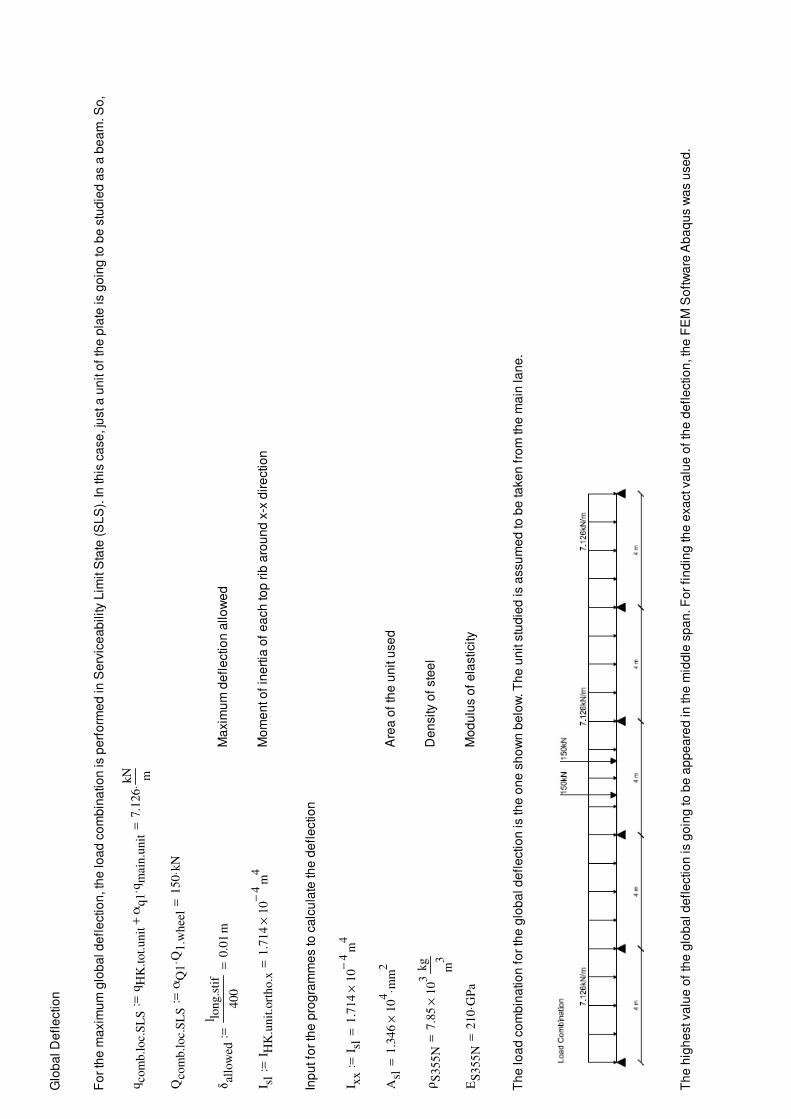
Glo

ba

l D

efl

ectio

n

Fo

r th

e m

axim

um

glo

ba

l d

efl

ectio

n, th

e lo

ad

co

mb

ina

tio

n is p

erf

orm

ed

in

Se

rvic

ea

bility L

imit S

tate

(S

LS

). In

th

is c

ase

, ju

st a

un

it o

f th

e p

late

is g

oin

g to

be

stu

die

d a

s a

be

am

. S

o,

qco

mb

.loc.

SL

SqH

K.t

ot.

un

itα

q1

qm

ain

.un

it⋅

+7

.12

6kN m

⋅=

:=

Qco

mb

.loc.

SL

Sα

Q1

Q1

.wh

eel

⋅1

50

kN

⋅=

:=

δal

low

ed

l lon

g.s

tif

40

00

.01

m=

:=

Ma

xim

um

de

fle

ctio

n a

llo

we

d

I sl

I HK

.un

it.o

rth

o.x

1.7

14

10

4−

×m

4=

:=

Mo

me

nt o

f in

ert

ia o

f e

ach

to

p r

ib a

rou

nd

x-x

dir

ectio

n

Inp

ut fo

r th

e p

rog

ram

me

s to

ca

lcu

late

th

e d

efl

ectio

n

I xx

I sl

1.7

14

10

4−

×m

4=

:=

Asl

1.3

46

10

4×

mm

2⋅

=A

rea

of

the

un

it u

se

d

ρS

35

5N

7.8

51

03

×

kg

m3

=D

en

sity o

f ste

el

ES

35

5N

21

0G

Pa

⋅=

Mo

du

lus o

f e

lasticity

Th

e lo

ad

co

mb

ina

tio

n f

or

the

glo

ba

l d

efl

ectio

n is th

e o

ne

sh

ow

n b

elo

w. T

he

un

it s

tud

ied

is a

ssu

me

d to

be

ta

ke

n f

rom

th

e m

ain

la

ne

.

Th

e h

igh

est va

lue

of

the

glo

ba

l d

efl

ectio

n is g

oin

g to

be

ap

pe

are

d in

th

e m

idd

le s

pa

n. F

or

fin

din

g th

e e

xa

ct va

lue

of

the

de

fle

ctio

n, th

e F

EM

So

ftw

are

Ab

aq

us w

as u

se

d.

Inp

ut fo

r th

e c

alc

ula

tio

n o

f th

e g

lob

al d

efl

ectio

n in

Ab

aq

us

Asl

0.0

13

m2

=

I HK

.un

it.o

rth

o.x

1.7

14

10

4−

×m

4⋅

=M

om

en

t o

f in

ert

ia a

rou

nd

th

e x

-x a

xis

I HK

.un

it.o

rth

o.z

2.1

86

10

4−

×m

4⋅

=M

om

en

t o

f in

ert

ia a

rou

nd

th

e z

-z a

xis

I HK

.un

it.o

rth

o.x

z3

.89

21

05

−×

m4

=P

rod

uct o

f in

ert

ia

Th

e r

esu

lts o

f A

ba

qu

s a

re s

ho

wn

be

low

.

So

, th

e m

axim

um

de

fle

ctio

n o

f th

e u

nit is c

on

cid

ere

d to

be

:

δm

ax.o

rth

o5

.26

1m

m:=

δm

ax.o

rth

oδal

low

ed≤

1=

In o

rde

r to

fin

d th

e m

axim

um

de

fle

ctio

n, a

n a

ssu

mp

tio

n h

as b

ee

n m

ad

e th

at th

e w

ho

le lo

ad

fro

m th

e tru

ck w

he

el is

ca

rrie

d b

y o

ne

un

it. H

ow

eve

r, in

re

ality

we

ha

ve

a m

om

en

t d

istr

ibu

tio

n in

th

e p

so

th

e a

ctu

all lo

ad

ca

rrie

d b

y e

ach

un

it is a

rou

nd

90

% o

f w

ha

t it is c

alc

ula

ted

fo

r o

ur

ca

se

. B

y a

ssu

min

g th

at th

e w

ho

le w

he

el tr

ack is ta

ke

n b

y o

ne

un

it, th

e s

tud

y r

em

ain

s o

n th

e s

afe

sif

e.

Glo

bal D

eflect

ion o

f th

e o

rthotr

opic

bridge d

eck

Local D

eflection

Ma

xim

um

lo

ca

l d

efl

ectio

n a

llo

we

d

δlo

cal.

allo

wed

.1

l HK

.rib

.top

.f.t

op

40

07

.65

51

04

−×

m=

:=

Ma

xim

um

de

fle

ctio

n b

etw

ee

n th

e w

eb

s o

f o

ne

lo

ng

itu

din

al stiff

en

er

δlo

cal.

allo

wed

.2

bH

K.f

.top

l HK

.rib

.top

.f.t

op

−

40

07

.34

51

04

−×

m=

:=

Ma

xim

um

de

fle

ctio

n b

etw

ee

n th

e w

eb

s o

f d

iffe

ren

t lo

ng

itu

din

al stiff

en

ers

δlo

cal.

allo

wed

minδlo

cal.

allo

wed

.1δlo

cal.

allo

wed

.2,

()

7.3

45

10

4−

×m

=:=

Ma

xim

um

de

fle

ctio

n a

llo

we

d

Pe

rma

ne

nt lo

ad

s

Fo

r th

e s

elf

-we

igh

t, ju

st th

e to

p f

lan

ge

is ta

ke

n in

to c

on

sid

era

tio

n a

s th

e in

ve

stig

atio

n o

f th

e lo

ca

l d

efl

ectio

n is c

arr

ied

ou

t b

etw

ee

n th

e lo

ng

itu

din

al stiff

en

ers

an

d b

etw

ee

n th

e w

eb

s o

f e

ach

lon

gid

utin

al stiff

en

er.

qH

K.f

.top

t HK

.f.t

opρ

S3

55

N⋅

g⋅

0.9

24

kN

m2

⋅=

:=

Se

lf-w

eig

ht o

f th

e to

p f

lan

ge

pe

r sq

ua

re m

ete

r o

f th

e c

on

str

uctio

n

qH

K.a

spa d

t cover

⋅1

.15

kN

m2

⋅=

:=

Asp

ha

lt c

ove

r p

er

sq

ua

re m

ete

r o

f th

e c

on

str

uctio

n

Lo

ad

co

nsid

ere

d f

or

the

lo

ca

l d

efl

ectio

n

qco

mb

.loca

l.1

qH

K.f

.top

qH

K.a

sp+

αq

1qm

ain

⋅+

()

1⋅

m:=

Un

ifo

rmly

dis

trib

ute

d lo

ad

pe

r u

nit w

idth

fo

r th

e m

ain

la

ne

qco

mb

.loca

l.1

11

.07

4kN m

⋅=

qco

mb

.loca

l.2

qH

K.f

.top

qH

K.a

sp+

αq

1qoth

er⋅

+(

)1

⋅m

:=

qco

mb

.loca

l.2

4.5

74

kN m

⋅=

Un

ifo

rmly

dis

trib

ute

d lo

ad

pe

r u

nit w

idth

fo

r th

e o

the

r la

ne

s

Qco

mb

.loca

l.1

αQ

1Q

1.w

hee

l1

50

kN

⋅=

:=

Qco

mb

.loca

l.2

αQ

1Q

2.w

hee

l⋅

10

0kN

⋅=

:=

bw

hee

l0

.4m

:=

Wid

th o

f th

e w

he

el

bw

hee

l.p

lbw

hee

l2

t cover

⋅+

0.5

m=

:=

Wid

th o

f th

e w

he

el o

n th

e to

p o

f th

e p

late

qco

mb

.wh

eel.

loca

l.1

Qco

mb

.loca

l.1

bw

hee

l.p

l

30

0kN m

⋅=

:=

Dis

trib

ute

d lo

ad

s o

f th

e w

he

els

in

0.5

m

qco

mb

.wh

eel.

loca

l.2

Qco

mb

.loca

l.2

bw

hee

l.p

l

20

0kN m

⋅=

:=

Th

e in

itia

l lo

ad

co

mb

ina

tio

n is:

Ho

we

ve

r, f

or

the

lo

ca

l b

ucklin

g, it is g

oin

g to

be

assu

me

d th

at th

e c

on

ce

ntr

ate

d lo

ad

is d

istr

ibu

ted

in

an

are

a e

qu

al w

ith

th

e w

idth

of

the

wh

ee

l o

n th

e s

urf

ace

of

the

to

p p

late

. M

ore

ove

r, th

eco

nce

ntr

ate

d lo

ad

s a

ctin

g n

ot b

etw

ee

n th

e w

eb

s o

f o

ne

lo

ng

itu

din

al stiff

en

er

bu

t in

th

e p

art

s o

f th

e p

late

be

twe

en

lo

ng

itu

din

al stiff

en

ers

ha

ve

fa

vo

uri

te c

on

trib

utio

n in

te

rms o

f lo

ca

l b

ucklin

g;

the

refo

re, th

ey c

an

be

ne

gle

cte

d. S

o, th

e f

ina

l lo

ad

co

mb

ina

tio

n is th

e o

ne

sh

ow

n b

elo

w.

Th

e m

od

el in

Ab

aq

us is c

on

sid

ere

d to

be

a s

imp

le b

ea

m w

ith

a w

idth

of

on

e m

ete

r, w

hile

hin

ge

s a

re u

se

d in

th

e p

lace

s w

he

re th

e w

eb

s a

re lo

ca

ted

, a

s s

ho

wn

in

th

e p

ictu

re b

elo

w. T

his

is n

ot

exa

ctly w

ha

t is

ha

pp

en

ing

in

re

ality

, a

s a

pa

rt f

rom

lo

ca

l b

ucklin

g, th

e p

late

will a

lso

bu

ckle

glo

ba

lly a

nd

th

e w

eb

s a

re g

oin

g to

ap

pe

ar

co

mp

ressiv

e d

efl

ectio

n if

the

y d

o n

ot b

uckle

th

em

se

lve

s.

Ho

we

ve

r, it is

an

ad

eq

ua

te a

ssu

mp

tio

n f

or

stu

dyin

g th

e lo

ca

l b

ucklin

g o

f th

e d

iffe

ren

t p

art

s o

f th

e b

rid

ge

de

ck. T

he

be

am

is lo

ad

ed

as illu

str

ate

d in

th

e f

igu

re a

bo

ve

.

Th

e lo

ca

l d

efl

ectio

n o

f th

e o

rth

otr

op

ic d

eck in

th

at ca

se

is 0

.31

8m

m

As th

e d

istr

ibu

ted

lo

ad

in

th

e p

art

be

twe

en

th

e tw

o e

xa

min

ed

stiff

en

ers

ca

use

s f

avo

uri

te c

on

trib

utio

n f

or

the

lo

ca

l b

ucklin

g, th

e d

istr

ibu

ted

lo

ad

of

the

wh

ee

ls o

f th

e tru

cks h

as b

ee

n r

elo

ca

ted

lik

eb

elo

w.

In th

at ca

se

, th

e lo

ca

l d

efl

ectio

n is b

igg

er, a

s e

xp

ecte

d, a

nd

it h

as a

ma

xim

um

va

lue

eq

ua

l to

0.4

12

mm

.

So

, th

e lo

ca

l d

efl

ectio

n is e

qu

al w

ith

δlo

cal.

max

4.1

21

04

−m

⋅:=

Ma

xim

um

lo

ca

l d

efl

ectio

n in

th

e c

om

pre

ssio

n f

lan

ge

Th

e lo

ca

l d

efl

ectio

n is lo

we

r th

an

th

e a

llo

we

d v

alu

eδlo

cal.

max

δlo

cal.

allo

wed

<1

=

Local D

eflection

SSE

Ste

el S

an

dw

ich

Ele

me

nt

He

igh

t o

f th

e c

ross-s

ectio

n

hss

phc.

ssp

t f.t

op

,

t f.b

ot

,

t c.s

sp,

()

hc.

ssp

t f.t

op

2+

t f.b

ot

2+

2t c

.ssp

2+

:=

Le

ng

th o

f th

e in

clin

ed

le

g o

f th

e c

ore

l i.s

sphc.

sspα

ssp

,

()

hc.

ssp

sinα

ssp

()

:=

Le

ng

th o

f co

rru

ga

tio

n o

pe

nin

g

l bu

ckhc.

sspα

ssp

,

f ssp

,

()

2l i

.ssp

hc.

sspα

ssp

,

()

cosα

ssp

()

⋅f s

sp+

:=

Ha

lf o

f th

e c

orr

ug

atio

n p

itch

pss

phc.

sspα

ssp

,

f ssp

,

()

f ssp 2

l bu

ckhc.

sspα

ssp

,

f ssp

,

()

2+

:=

Le

ng

th o

f cro

ss-s

ectio

n

l ssp

hc.

sspα

ssp

,

f ssp

,

()

2pss

phc.

sspα

ssp

,

f ssp

,

()

⋅:=

Co

nfi

gu

ratio

n r

atio

s

hc_

tchc.

ssp

t c.s

sp,

()

hc.

ssp

t c.s

sp

:=

p_

hc

hc.

sspα

ssp

,

f ssp

,

()

pss

phc.

sspα

ssp

,

f ssp

,

()

hc.

ssp

:=

Are

as

Af.

top

t f.t

op

hc.

ssp

,

αss

p,

f ssp

,

()

t f.t

op

l ssp

hc.

sspα

ssp

,

f ssp

,

()

⋅:=

Are

a o

f to

p f

lan

ge

s

Af.

bot

t f.b

ot

hc.

ssp

,

αss

p,

f ssp

,

()

t f.b

ot

l ssp

hc.

sspα

ssp

,

f ssp

,

()

⋅:=

Are

a o

f b

otto

m f

lan

ge

Are

a o

f th

e c

ore

Ac.

ssp

t c.s

sphc.

ssp

,

αss

p,

f ssp

,

()

2f s

sp⋅

t c.s

sp⋅

2t c

.ssp

⋅l i

.ssp

hc.

sspα

ssp

,

()

⋅+

:=

Are

a o

f th

e c

ore

pe

r u

nit w

idth

AC

.ssp

t c.s

sphc.

ssp

,

αss

p,

f ssp

,

()

Ac.

ssp

t c.s

sphc.

ssp

,

αss

p,

f ssp

,

()

l ssp

hc.

sspα

ssp

,

f ssp

,

()

:=

To

tal A

rea

Ato

t.ss

phc.

ssp

t f.t

op

,

t f.b

ot

,

t c.s

sp,

αss

p,

f ssp

,

()

Af.

top

t f.t

op

hc.

ssp

,

αss

p,

f ssp

,

()

Af.

bot

t f.b

ot

hc.

ssp

,

αss

p,

f ssp

,

()

+A

c.ss

pt c

.ssp

hc.

ssp

,

αss

p,

f ssp

,

()

+:=

To

tal a

rea

pe

r u

nit w

idth

[m

]

Ass

phc.

ssp

t f.t

op

,

t f.b

ot

,

t c.s

sp,

αss

p,

f ssp

,

()

Ato

t.ss

phc.

ssp

t f.t

op

,

t f.b

ot

,

t c.s

sp,

αss

p,

f ssp

,

()

l ssp

hc.

sspα

ssp

,

f ssp

,

()

:=

To

tal w

eig

ht o

f th

e s

ectio

n

Gss

phc.

ssp

t f.t

op

,

t f.b

ot

,

t c.s

sp,

αss

p,

f ssp

,

()

Ass

phc.

ssp

t f.t

op

,

t f.b

ot

,

t c.s

sp,

αss

p,

f ssp

,

()ρ

S3

55

N⋅

:=

Ne

utr

al A

xis

of

the

ste

el sa

nd

wic

h e

lem

en

t (d

ista

nce

fro

m th

e to

p)

z na.

ssp

hc.

ssp

t f.t

op

,

t f.b

ot

,

t c.s

sp,

αss

p,

f ssp

,

()

t c.s

spf s

sp⋅

t f.t

op

2

t c.s

sp

2+

⋅

2t c

.ssp

⋅l i

.ssp

hc.

sspα

ssp

,

()

⋅

hc.

ssp

2

t f.t

op

2+

t c.s

sp

2+

⋅

+

...

t c.s

spf s

sp⋅

t f.t

op

2

t c.s

sp

2+

hc.

ssp

+

⋅

+

...

Af.

bot

t f.b

ot

hc.

ssp

,

αss

p,

f ssp

,

()

hss

phc.

ssp

t f.t

op

,

t f.b

ot

,

t c.s

sp,

()

()

⋅+

...

A

tot.

ssp

hc.

ssp

t f.t

op

,

t f.b

ot

,

t c.s

sp,

αss

p,

f ssp

,

()

:=

Mo

me

nt o

f in

ert

ia in

X-

dir

ectio

n

Mo

me

nt o

f in

ert

ia f

or

the

to

p f

lan

ge

I f.t

op

.ssp

.xhc.

ssp

t f.t

op

,

t f.b

ot

,

t c.s

sp,

αss

p,

f ssp

,

()

l ssp

hc.

sspα

ssp

,

f ssp

,

()

t f.t

op

3⋅

12

l ssp

hc.

sspα

ssp

,

f ssp

,

()

t f.t

op

⋅z n

a.ss

phc.

ssp

t f.t

op

,

t f.b

ot

,

t c.s

sp,

αss

p,

f ssp

,

()

()2

⋅+

:=

Mo

me

nt o

f in

ert

ia f

or

the

to

p h

ori

so

nta

l p

art

of

the

co

re

I c.t

op

.ssp

.xhc.

ssp

t f.t

op

,

t f.b

ot

,

t c.s

sp,

αss

p,

f ssp

,

()

f ssp

t c.s

sp3

⋅ 12

f ssp

t c.s

sp⋅

z na.

ssp

hc.

ssp

t f.t

op

,

t f.b

ot

,

t c.s

sp,

αss

p,

f ssp

,

()

t f.t

op

2−

t c.s

sp

2−

2

⋅+

:=

Mo

me

nt o

f in

ert

ia f

or

the

in

clin

ed

pa

rt o

f th

e c

ore

I in

c.ss

p.x

hc.

ssp

t f.t

op

,

t f.b

ot

,

t c.s

sp,

αss

p,

f ssp

,

()

2t c

.ssp

l i.s

sphc.

sspα

ssp

,

()3

⋅

12

⋅si

nα

ssp

()2

⋅

2t c

.ssp

l i.s

sphc.

sspα

ssp

,

()

⋅

t f.t

op

2

t c.s

sp

2+

hc.

ssp

2+

z na.

ssp

hc.

ssp

t f.t

op

,

t f.b

ot

,

t c.s

sp,

αss

p,

f ssp

,

()

−+

...

2

⋅+

...

:=

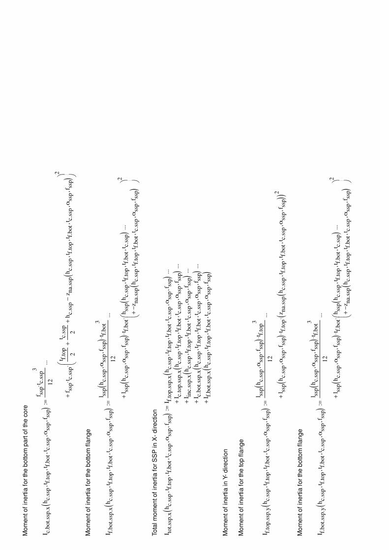
Mo

me

nt o

f in

ert

ia f

or

the

bo

tto

m p

art

of

the

co

re

I c.b

ot.

ssp

.xhc.

ssp

t f.t

op

,

t f.b

ot

,

t c.s

sp,

αss

p,

f ssp

,

()

f ssp

t c.s

sp3

⋅ 12

f ssp

t c.s

sp⋅

t f.t

op

2

t c.s

sp

2+

hc.

ssp

+z n

a.ss

phc.

ssp

t f.t

op

,

t f.b

ot

,

t c.s

sp,

αss

p,

f ssp

,

()

−

2

⋅+

...

:=

Mo

me

nt o

f in

ert

ia f

or

the

bo

tto

m f

lan

ge

I f.b

ot.

ssp

.xhc.

ssp

t f.t

op

,

t f.b

ot

,

t c.s

sp,

αss

p,

f ssp

,

()

l ssp

hc.

sspα

ssp

,

f ssp

,

()

t f.b

ot3

⋅

12

l ssp

hc.

sspα

ssp

,

f ssp

,

()

t f.b

ot

⋅hss

phc.

ssp

t f.t

op

,

t f.b

ot

,

t c.s

sp,

()

z na.

ssp

hc.

ssp

t f.t

op

,

t f.b

ot

,

t c.s

sp,

αss

p,

f ssp

,

()

−+

...

2⋅

+

...

:=

To

tal m

om

en

t o

f in

ert

ia f

or

SS

P in

X-

dir

ectio

n

I tot.

ssp

.xhc.

ssp

t f.t

op

,

t f.b

ot

,

t c.s

sp,

αss

p,

f ssp

,

()

I f.t

op

.ssp

.xhc.

ssp

t f.t

op

,

t f.b

ot

,

t c.s

sp,

αss

p,

f ssp

,

()

I c.t

op

.ssp

.xhc.

ssp

t f.t

op

,

t f.b

ot

,

t c.s

sp,

αss

p,

f ssp

,

()

+

...

I in

c.ss

p.x

hc.

ssp

t f.t

op

,

t f.b

ot

,

t c.s

sp,

αss

p,

f ssp

,

()

+

...

I c.b

ot.

ssp

.xhc.

ssp

t f.t

op

,

t f.b

ot

,

t c.s

sp,

αss

p,

f ssp

,

()

+

...

I f.b

ot.

ssp

.xhc.

ssp

t f.t

op

,

t f.b

ot

,

t c.s

sp,

αss

p,

f ssp

,

()

+

...

:=

Mo

me

nt o

f in

ert

ia in

Y-

dir

ectio

n

Mo

me

nt o

f in

ert

ia f

or

the

to

p f

lan

ge

I f.t

op

.ssp

.yhc.

ssp

t f.t

op

,

t f.b

ot

,

t c.s

sp,

αss

p,

f ssp

,

()

l ssp

hc.

sspα

ssp

,

f ssp

,

()

t f.t

op

3⋅

12

l ssp

hc.

sspα

ssp

,

f ssp

,

()

t f.t

op

⋅z n

a.ss

phc.

ssp

t f.t

op

,

t f.b

ot

,

t c.s

sp,

αss

p,

f ssp

,

()

()2

⋅+

...

:=

Mo

me

nt o

f in

ert

ia f

or

the

bo

tto

m f

lan

ge

I f.b

ot.

ssp

.yhc.

ssp

t f.t

op

,

t f.b

ot

,

t c.s

sp,

αss

p,

f ssp

,

()

l ssp

hc.

sspα

ssp

,

f ssp

,

()

t f.b

ot3

⋅

12

l ssp

hc.

sspα

ssp

,

f ssp

,

()

t f.b

ot

⋅hss

phc.

ssp

t f.t

op

,

t f.b

ot

,

t c.s

sp,

()

z na.

ssp

hc.

ssp

t f.t

op

,

t f.b

ot

,

t c.s

sp,

αss

p,

f ssp

,

()

−+

...

2⋅

+

...

:=

Mo

me

nt o

f in

ert

ia f

or

the

to

p h

ori

so

nta

l p

art

of

the

co

re

I c.t

op

.ssp

.yhc.

ssp

t f.t

op

,

t f.b

ot

,

t c.s

sp,

αss

p,

f ssp

,

()

f ssp

t c.s

sp3

⋅ 12

f ssp

t c.s

sp⋅

z na.

ssp

hc.

ssp

t f.t

op

,

t f.b

ot

,

t c.s

sp,

αss

p,

f ssp

,

()

t f.t

op

2−

t c.s

sp

2−

2

⋅+

:=

Mo

me

nt o

f in

ert

ia f

or

the

bo

tto

m p

art

of

the

co

re

I c.b

ot.

ssp

.yhc.

ssp

t f.t

op

,

t f.b

ot

,

t c.s

sp,

αss

p,

f ssp

,

()

f ssp

t c.s

sp3

⋅ 12

f ssp

t c.s

sp⋅

t f.t

op

2

t c.s

sp

2+

hc.

ssp

+z n

a.ss

phc.

ssp

t f.t

op

,

t f.b

ot

,

t c.s

sp,

αss

p,

f ssp

,

()

−

2

⋅+

...

:=

To

tal m

om

en

t o

f in

ert

ia f

or

SS

P in

Y-

dir

ectio

n

I tot.

ssp

.yhc.

ssp

t f.t

op

,

t f.b

ot

,

t c.s

sp,

αss

p,

f ssp

,

()

I f.t

op

.ssp

.yhc.

ssp

t f.t

op

,

t f.b

ot

,

t c.s

sp,

αss

p,

f ssp

,

()

I f.b

ot.

ssp

.yhc.

ssp

t f.t

op

,

t f.b

ot

,

t c.s

sp,

αss

p,

f ssp

,

()

+

...

I c.t

op

.ssp

.yhc.

ssp

t f.t

op

,

t f.b

ot

,

t c.s

sp,

αss

p,

f ssp

,

()

+

...

I c.b

ot.

ssp

.yhc.

ssp

t f.t

op

,

t f.b

ot

,

t c.s

sp,

αss

p,

f ssp

,

()

+

...

:=

Mo

me

nt o

f in

ert

ia in

X a

nd

Y d

ire

ctio

n p

er

un

it w

idth

[m

^3]

I ssp

.xhc.

ssp

t f.t

op

,

t f.b

ot

,

t c.s

sp,

αss

p,

f ssp

,

()

I tot.

ssp

.xhc.

ssp

t f.t

op

,

t f.b

ot

,

t c.s

sp,

αss

p,

f ssp

,

()

l ssp

hc.

sspα

ssp

,

f ssp

,

()

:=

I ssp

.yhc.

ssp

t f.t

op

,

t f.b

ot

,

t c.s

sp,

αss

p,

f ssp

,

()

I tot.

ssp

.yhc.

ssp

t f.t

op

,

t f.b

ot

,

t c.s

sp,

αss

p,

f ssp

,

()

l ssp

hc.

sspα

ssp

,

f ssp

,

()

:=

Be

nd

ing

Stiff

ne

ss p

er

un

it w

idth

Be

nd

ing

stiff

ne

ss in

th

e s

tiff

dir

ectio

n p

er

un

it w

idth

Dx

.ssp

hc.

ssp

t f.t

op

,

t f.b

ot

,

t c.s

sp,

αss

p,

f ssp

,

()

ES

35

5N

I ssp

.xhc.

ssp

t f.t

op

,

t f.b

ot

,

t c.s

sp,

αss

p,

f ssp

,

()

⋅:=

Be

nd

ing

stiff

ne

ss in

th

e w

ea

k d

ire

ctio

n p

er

un

it w

idth

Dy.s

sphc.

ssp

t f.t

op

,

t f.b

ot

,

t c.s

sp,

αss

p,

f ssp

,

()

ES

35

5N

I ssp

.yhc.

ssp

t f.t

op

,

t f.b

ot

,

t c.s

sp,

αss

p,

f ssp

,

()

⋅

1ν

21

ES

35

5N

I ssp

.yhc.

ssp

t f.t

op

,

t f.b

ot

,

t c.s

sp,

αss

p,

f ssp

,

()

⋅

Dx

.ssp

hc.

ssp

t f.t

op

,

t f.b

ot

,

t c.s

sp,

αss

p,

f ssp

,

()

−

−

:=

To

rsio

na

l S

tiff

ne

ss p

er

un

it w

idth

(a

cco

rdin

g to

Lib

ova

-Hu

bka

)

GA

hc.

ssp

t f.t

op

,

t f.b

ot

,

t c.s

sp,

αss

p,

f ssp

,

()

Gc

t f.t

op

⋅

Gc

t c.s

sp2

⋅

AC

.ssp

t c.s

sphc.

ssp

,

αss

p,

f ssp

,

()

+G

ct f

.bot

⋅+

:=

kc

1 21

A1

A2

−

2p

⋅h

⋅

+

⋅

=

kc

hc.

ssp

t f.t

op

,

t f.b

ot

,

t c.s

sp,

()

1 21

t f.b

ot

t f.t

op

−

2hss

phc.

ssp

t f.t

op

,

t f.b

ot

,

t c.s

sp,

()

⋅

+

:=

kG

Jhc.

ssp

t f.t

op

,

t f.b

ot

,

t c.s

sp,

αss

p,

f ssp

,

()

Gc

t c.s

sp2

⋅kc

hc.

ssp

t f.t

op

,

t f.b

ot

,

t c.s

sp,

()

⋅

AC

.ssp

t c.s

sphc.

ssp

,

αss

p,

f ssp

,

()

Gc

t f.b

ot

⋅+

GA

hc.

ssp

t f.t

op

,

t f.b

ot

,

t c.s

sp,

αss

p,

f ssp

,

()

:=

GJ

hc.

ssp

t f.t

op

,

t f.b

ot

,

t c.s

sp,

αss

p,

f ssp

,

()

Gc

t f.t

op

⋅kG

Jhc.

ssp

t f.t

op

,

t f.b

ot

,

t c.s

sp,

αss

p,

f ssp

,

()2

⋅

Gc

t c.s

sp2

⋅

AC

.ssp

t c.s

sphc.

ssp

,

αss

p,

f ssp

,

()

kG

Jhc.

ssp

t f.t

op

,

t f.b

ot

,

t c.s

sp,

αss

p,

f ssp

,

()

kc

hc.

ssp

t f.t

op

,

t f.b

ot

,

t c.s

sp,

()

−+

...

2⋅

+

...

Gc

t f.b

ot

⋅1

kG

Jhc.

ssp

t f.t

op

,

t f.b

ot

,

t c.s

sp,

αss

p,

f ssp

,

()

−(

)2⋅

+

...

hss

phc.

ssp

t f.t

op

,

t f.b

ot

,

t c.s

sp,

()2

⋅:=

Dx

y.s

sphc.

ssp

t f.t

op

,

t f.b

ot

,

t c.s

sp,

αss

p,

f ssp

,

()

2G

Jhc.

ssp

t f.t

op

,

t f.b

ot

,

t c.s

sp,

αss

p,

f ssp

,

()

⋅:=

Axia

l S

tiff

ne

ss p

er

un

it w

idth

Axia

l stiff

ne

ss in

th

e s

tro

ng

dir

ectio

n p

er

un

it w

idth

Ex

.ssp

hc.

ssp

t f.t

op

,

t f.b

ot

,

t c.s

sp,

αss

p,

f ssp

,

()

ES

35

5N

Ass

phc.

ssp

t f.t

op

,

t f.b

ot

,

t c.s

sp,

αss

p,

f ssp

,

()

⋅:=

Axia

l stiff

ne

ss in

th

e w

ea

k d

ire

ctio

n p

er

un

it w

idth

Ey.s

sphc.

ssp

t f.t

op

,

t f.b

ot

,

t c.s

sp,

αss

p,

f ssp

,

()

ES

35

5N

t f.t

op

t f.b

ot

+(

)⋅

1ν

21

ES

35

5N

t f.t

op

t f.b

ot

+(

)⋅

Ex

.ssp

hc.

ssp

t f.t

op

,

t f.b

ot

,

t c.s

sp,

αss

p,

f ssp

,

()

−

−

:=

Ho

rizo

nta

l sh

ea

r stiff

ne

ss p

er

un

it w

idth

Gx

yhc.

ssp

t f.t

op

,

t f.b

ot

,

t c.s

sp,

αss

p,

f ssp

,

()

GA

hc.

ssp

t f.t

op

,

t f.b

ot

,

t c.s

sp,

αss

p,

f ssp

,

()

:=

Dim

en

sio

ns n

ee

de

d f

or

DQ

x a

nd

DQ

y

Du

e to

sym

me

tric

al co

rru

ga

tio

n k

.y=

k.z

=1

an

d K

.Ay=

K.A

z=

0. M

ore

ove

r, w

e a

ssu

me

th

at R

c.1

=0

.

ky

1:=

kz

1:=

KA

y0

:=

KA

z0

:=

RC

10

mm

:=

a 1hc.

ssp

RC

1,

()

1kz 2

−

hc.

ssp

⋅R

C1

−:=

b1

hc.

sspα

ssp

,

f ssp

,

()

1ky 2

−

pss

phc.

sspα

ssp

,

f ssp

,

()

⋅

f ssp 2

−:=

c 1hc.

sspα

ssp

,

f ssp

,

RC

1,

()

a 1hc.

ssp

RC

1,

()2

b1

hc.

sspα

ssp

,

f ssp

,

()2

+

1 2

:=

α1

hc.

sspα

ssp

,

f ssp

,

RC

1,

()

atan

a 1hc.

ssp

RC

1,

()

b1

hc.

sspα

ssp

,

f ssp

,

()

:=

β1

hc.

sspα

ssp

,

f ssp

,

RC

1,

()

asin

RC

1

c 1hc.

sspα

ssp

,

f ssp

,

RC

1,

()

:=

d1

hc.

sspα

ssp

,

f ssp

,

RC

1,

()

c 1hc.

sspα

ssp

,

f ssp

,

RC

1,

()2

RC

12

−

1 2

:=

θhc.

sspα

ssp

,

f ssp

,

RC

1,

()

α1

hc.

sspα

ssp

,

f ssp

,

RC

1,

()

β1

hc.

sspα

ssp

,

f ssp

,

RC

1,

()

+:=

e 1hc.

sspα

ssp

,

f ssp

,

RC

1,

()

RC

1co

sθ

hc.

sspα

ssp

,

f ssp

,

RC

1,

()

()

⋅:=

g1

hc.

sspα

ssp

,

f ssp

,

RC

1,

()

RC

1si

nθ

hc.

sspα

ssp

,

f ssp

,

RC

1,

()

()

⋅:=

l 1hc.

sspα

ssp

,

f ssp

,

RC

1,

()

a 1hc.

ssp

RC

1,

()

e 1hc.

sspα

ssp

,

f ssp

,

RC

1,

()

+:=

k1

hc.

sspα

ssp

,

f ssp

,

RC

1,

()

b1

hc.

sspα

ssp

,

f ssp

,

()

g1

hc.

sspα

ssp

,

f ssp

,

RC

1,

()

−:=

Le

ng

ht o

f o

ne

co

rru

ga

tio

n le

g

l shc.

sspα

ssp

,

f ssp

,

RC

1,

()

f ssp

2.R

C1θ

hc.

sspα

ssp

,

f ssp

,

RC

1,

()

⋅+

2d1

hc.

sspα

ssp

,

f ssp

,

RC

1,

()

⋅+

:=

Tra

nsve

rse

sh

ea

r stiff

ne

ss p

ara

lle

l to

th

e c

orr

ug

atio

n p

er

un

it w

idth

, D

Qx

Th

e tra

nsve

rse

sh

ea

r stiff

ne

ss in

th

e s

tro

ng

dir

ectio

n is e

qu

al w

ith

:

DQ

x

Gc

t c.s

sp2

⋅

Ac.

ssp

.x

hss

p

pss

p

2

⋅=

So

,

Ac.

ssp

.xhc.

ssp

t c.s

sp,

αss

p,

f ssp

,

RC

1,

()

l shc.

sspα

ssp

,

f ssp

,

RC

1,

()

t c.s

sp⋅

pss

phc.

sspα

ssp

,

f ssp

,

()

:=

Are

a p

er

un

it w

idth

of

the

co

rru

ga

ted

co

re

DQ

xhc.

ssp

t f.t

op

,

t f.b

ot

,

t c.s

sp,

αss

p,

f ssp

,

()

Gc

t c.s

sp2

⋅

Ac.

ssp

.xhc.

ssp

t c.s

sp,

αss

p,

f ssp

,

RC

1,

()

hss

phc.

ssp

t f.t

op

,

t f.b

ot

,

t c.s

sp,

()

pss

phc.

sspα

ssp

,

f ssp

,

()

2

⋅:=

Tra

nsve

rse

sh

ea

r stiff

ne

ss p

erp

en

dic

ula

r to

th

e c

orr

ug

atio

n p

er

un

it w

idth

, D

Qy

Th

e tra

nsve

rse

sh

ea

r stiff

ne

ss in

th

e w

ea

k d

ire

ctio

n is e

qu

al w

ith

:

DQ

yS

hss

p

ES

35

5N

1ν

c2−

⋅

t c hc

3

=

No

n-d

ime

nsio

na

l co

eff

icie

nt S

Th

e c

oe

ffic

ien

t S

is u

se

d to

ta

ke

in

to c

on

sid

era

tio

n th

e c

ore

sh

ap

e in

th

e w

ea

k d

ire

ctio

n. T

he

fo

rmu

las h

ave

be

en

ob

tain

ed

by p

ap

ers

"E

lastic C

on

sta

nts

fo

rC

orr

ug

ate

d-c

ore

Sa

nd

wic

h P

late

s"

by L

ibo

va

an

d H

ub

ka

an

d "

Ela

sto

-pla

stic A

na

lysis

of

Co

rru

ga

ted

Sa

nd

wic

h S

tee

l P

an

els

" b

y C

ha

ng

.

K e

xp

ressio

ns

KIz

hc.

sspα

ssp

,

f ssp

,

RC

1,

()

2 3

k1

hc.

sspα

ssp

,

f ssp

,

RC

1,

()

hc.

ssp

2

⋅

d1

hc.

sspα

ssp

,

f ssp

,

RC

1,

()

hc.

ssp

⋅

2 3

1 8

pss

phc.

sspα

ssp

,

f ssp

,

()

hc.

ssp

3

⋅

b1

hc.

sspα

ssp

,

f ssp

,

()

hc.

ssp

3

−

⋅

+

2R

C1

hc.

ssp

⋅

b1

hc.

sspα

ssp

,

f ssp

,

()

hc.

ssp

θhc.

sspα

ssp

,

f ssp

,

RC

1,

()

b1

hc.

sspα

ssp

,

f ssp

,

()

hc.

ssp

⋅2

RC

1

hc.

ssp

e 1hc.

sspα

ssp

,

f ssp

,

RC

1,

()

hc.

ssp

−

⋅

−

⋅

1 2θ

hc.

sspα

ssp

,

f ssp

,

RC

1,

()

RC

1

hc.

ssp

2

⋅

g1

hc.

sspα

ssp

,

f ssp

,

RC

1,

()

hc.

ssp

e 1hc.

sspα

ssp

,

f ssp

,

RC

1,

()

hc.

ssp

⋅−

⋅

+

...

⋅+

...

:=

KIy

zhc.

sspα

ssp

,

f ssp

,

RC

1,

()

2 3

l 1hc.

sspα

ssp

,

f ssp

,

RC

1,

()

hc.

ssp

⋅

k1

hc.

sspα

ssp

,

f ssp

,

RC

1,

()

hc.

ssp

⋅

d1

hc.

sspα

ssp

,

f ssp

,

RC

1,

()

hc.

ssp

⋅

1 2

1 4

pss

phc.

sspα

ssp

,

f ssp

,

()

hc.

ssp

2

⋅

b1

hc.

sspα

ssp

,

f ssp

,

()

hc.

ssp

2

−

⋅

+

...

2R

C1

hc.

ssp

⋅

a 1hc.

ssp

RC

1,

()

hc.

ssp

θhc.

sspα

ssp

,

f ssp

,

RC

1,

()

b1

hc.

sspα

ssp

,

f ssp

,

()

hc.

ssp

⋅

e 1hc.

sspα

ssp

,

f ssp

,

RC

1,

()

hc.

ssp

+

RC

1

hc.

ssp

−

⋅

g1

hc.

sspα

ssp

,

f ssp

,

RC

1,

()

hc.

ssp

b1

hc.

sspα

ssp

,

f ssp

,

()

hc.

ssp

1 2

g1

hc.

sspα

ssp

,

f ssp

,

RC

1,

()

hc.

ssp

⋅−

⋅

+

...

⋅+

...

:=

KIy

hc.

sspα

ssp

,

f ssp

,

RC

1,

()

2 3

l 1hc.

sspα

ssp

,

f ssp

,

RC

1,

()

hc.

ssp

2

⋅

d1

hc.

sspα

ssp

,

f ssp

,

RC

1,

()

hc.

ssp

⋅

1 4

f ssp

hc.

ssp

⋅+

2R

C1

hc.

ssp

⋅

a 1hc.

ssp

RC

1,

()

hc.

ssp

θhc.

sspα

ssp

,

f ssp

,

RC

1,

()

a 1hc.

ssp

RC

1,

()

hc.

ssp

⋅2

g1

hc.

sspα

ssp

,

f ssp

,

RC

1,

()

hc.

ssp

⋅+

⋅

1 2θ

hc.

sspα

ssp

,

f ssp

,

RC

1,

()

RC

1

hc.

ssp

2

⋅

g1

hc.

sspα

ssp

,

f ssp

,

RC

1,

()

hc.

ssp

e 1hc.

sspα

ssp

,

f ssp

,

RC

1,

()

hc.

ssp

⋅+

⋅

+

...

⋅+

...

:=

KL

hc.

sspα

ssp

,

f ssp

,

RC

1,

()

2d1

hc.

sspα

ssp

,

f ssp

,

RC

1,

()

hc.

ssp

⋅2θ

hc.

sspα

ssp

,

f ssp

,

RC

1,

()

⋅

RC

1

hc.

ssp

⋅+

f ssp

hc.

ssp

+:=

KL

yhc.

sspα

ssp

,

f ssp

,

RC

1,

()

f ssp

hc.

ssp

2d1

hc.

sspα

ssp

,

f ssp

,

RC

1,

()

hc.

ssp

⋅co

sθ

hc.

sspα

ssp

,

f ssp

,

RC

1,

()

()2

⋅+

RC

1

hc.

ssp

θhc.

sspα

ssp

,

f ssp

,

RC

1,

()

sinθ

hc.

sspα

ssp

,

f ssp

,

RC

1,

()

()

cosθ

hc.

sspα

ssp

,

f ssp

,

RC

1,

()

()

⋅+

()

⋅+

...

:=

KL

yz

hc.

sspα

ssp

,

f ssp

,

RC

1,

()

2d1

hc.

sspα

ssp

,

f ssp

,

RC

1,

()

hc.

ssp

sinθ

hc.

sspα

ssp

,

f ssp

,

RC

1,

()

()

⋅⋅

cosθ

hc.

sspα

ssp

,

f ssp

,

RC

1,

()

()

⋅

RC

1

hc.

ssp

sinθ

hc.

sspα

ssp

,

f ssp

,

RC

1,

()

()2

⋅+

...

:=

KL

zhc.

sspα

ssp

,

f ssp

,

RC

1,

()

2d1

hc.

sspα

ssp

,

f ssp

,

RC

1,

()

hc.

ssp

⋅si

nθ

hc.

sspα

ssp

,

f ssp

,

RC

1,

()

()2

⋅

RC

1

hc.

ssp

θhc.

sspα

ssp

,

f ssp

,

RC

1,

()

sinθ

hc.

sspα

ssp

,

f ssp

,

RC

1,

()

()

cosθ

hc.

sspα

ssp

,

f ssp

,

RC

1,

()

()

⋅−

()

⋅+

...

:=

C e

xp

ressio

ns

C1

hc.

ssp

t f.t

op

,

t c.s

sp,

αss

p,

f ssp

,

RC

1,

()

KL

hc.

sspα

ssp

,

f ssp

,

RC

1,

()

1 3

t c.s

sp

t f.t

op

3

⋅

pss

phc.

sspα

ssp

,

f ssp

,

()

hc.

ssp

⋅+

:=

C2

hc.

sspα

ssp

,

f ssp

,

RC

1,

()

ky 2

pss

phc.

sspα

ssp

,

f ssp

,

()

hc.

ssp

⋅K

Lhc.

sspα

ssp

,

f ssp

,

RC

1,

()

⋅:=

C3

hc.

ssp

t c.s

sp,

αss

p,

f ssp

,

RC

1,

()

KIz

hc.

sspα

ssp

,

f ssp

,

RC

1,

()

ky

pss

phc.

sspα

ssp

,

f ssp

,

()

hc.

ssp

⋅

ky 4

pss

phc.

sspα

ssp

,

f ssp

,

()

hc.

ssp

⋅K

Lhc.

sspα

ssp

,

f ssp

,

RC

1,

()

⋅

⋅

+

1 12

t c.s

sp

hc.

ssp

2

⋅K

Lz

hc.

sspα

ssp

,

f ssp

,

RC

1,

()

⋅+

...

:=

C4

hc.

ssp

t f.t

op

,

t c.s

sp,

αss

p,

f ssp

,

RC

1,

()

KIy

zhc.

sspα

ssp

,

f ssp

,

RC

1,

()

1 2kz

1t f

.top

t c.s

sp

+

t c.s

sp

hc.

ssp

⋅+

⋅

ky 2

pss

phc.

sspα

ssp

,

f ssp

,

()

hc.

ssp

⋅K

Lhc.

sspα

ssp

,

f ssp

,

RC

1,

()

⋅

⋅

+

...

1 12

−

t c.s

sp

hc.

ssp

2

⋅K

Lyz

hc.

sspα

ssp

,

f ssp

,

RC

1,

()

⋅+

...

:=

C5

hc.

ssp

t f.t

op

,

t c.s

sp,

αss

p,

f ssp

,

RC

1,

()

1 2kz

1t f

.top

t c.s

sp

+

t c.s

sp

hc.

ssp

⋅+

⋅

KL

hc.

sspα

ssp

,

f ssp

,

RC

1,

()

⋅:=

C6

hc.

ssp

t f.t

op

,

t c.s

sp,

αss

p,

f ssp

,

RC

1,

()

KIy

hc.

sspα

ssp

,

f ssp

,

RC

1,

()

kz

1t f

.top

t c.s

sp

+

t c.s

sp

hc.

ssp

⋅+

1 4kz

1t f

.top

t c.s

sp

+

t c.s

sp

hc.

ssp

⋅+

⋅

KL

hc.

sspα

ssp

,

f ssp

,

RC

1,

()

⋅

⋅

+

...

1 12

t c.s

sp

hc.

ssp

2

⋅K

Ly

hc.

sspα

ssp

,

f ssp

,

RC

1,

()

⋅+

...

:=

C7

t f.b

ot

t c.s

sp,

()

t f.b

ot

t c.s

sp

3

:=

S1

hc.

ssp

t f.t

op

,

t f.b

ot

,

t c.s

sp,

αss

p,

f ssp

,

RC

1,

()

pss

phc.

sspα

ssp

,

f ssp

,

()

hc.

ssp

C1

hc.

ssp

t f.t

op

,

t c.s

sp,

αss

p,

f ssp

,

RC

1,

()

C4

hc.

ssp

t f.t

op

,

t c.s

sp,

αss

p,

f ssp

,

RC

1,

()

⋅

C2

hc.

sspα

ssp

,

f ssp

,

RC

1,

()

−C

5hc.

ssp

t f.t

op

,

t c.s

sp,

αss

p,

f ssp

,

RC

1,

()

⋅+

...

⋅

C2

hc.

sspα

ssp

,

f ssp

,

RC

1,

()

C4

hc.

ssp

t f.t

op

,

t c.s

sp,

αss

p,

f ssp

,

RC

1,

()

⋅

C3

hc.

ssp

t c.s

sp,

αss

p,

f ssp

,

RC

1,

()

−C

5hc.

ssp

t f.t

op

,

t c.s

sp,

αss

p,

f ssp

,

RC

1,

()

⋅+

...

−+

...

:=

S2

hc.

ssp

t f.t

op

,

t f.b

ot

,

t c.s

sp,

αss

p,

f ssp

,

RC

1,

()

C1

hc.

ssp

t f.t

op

,

t c.s

sp,

αss

p,

f ssp

,

RC

1,

()

C4

hc.

ssp

t f.t

op

,

t c.s

sp,

αss

p,

f ssp

,

RC

1,

()

⋅

2−

C2

hc.

sspα

ssp

,

f ssp

,

RC

1,

()

⋅C

5hc.

ssp

t f.t

op

,

t c.s

sp,

αss

p,

f ssp

,

RC

1,

()

⋅+

...

:=

S3

hc.

ssp

t f.t

op

,

t f.b

ot

,

t c.s

sp,

αss

p,

f ssp

,

RC

1,

()

C4

hc.

ssp

t f.t

op

,

t c.s

sp,

αss

p,

f ssp

,

RC

1,

()

S2

hc.

ssp

t f.t

op

,

t f.b

ot

,

t c.s

sp,

αss

p,

f ssp

,

RC

1,

()

⋅

C3

hc.

ssp

t c.s

sp,

αss

p,

f ssp

,

RC

1,

()

C5

hc.

ssp

t f.t

op

,

t c.s

sp,

αss

p,

f ssp

,

RC

1,

()2

⋅+

...

C6

hc.

ssp

t f.t

op

,

t c.s

sp,

αss

p,

f ssp

,

RC

1,

()

−C

1hc.

ssp

t f.t

op

,

t c.s

sp,

αss

p,

f ssp

,

RC

1,

()

C3

hc.

ssp

t c.s

sp,

αss

p,

f ssp

,

RC

1,

()

⋅

C2

hc.

sspα

ssp

,

f ssp

,

RC

1,

()2

−+

...

⋅+

...

:=

S4

hc.

ssp

t f.t

op

,

t f.b

ot

,

t c.s

sp,

αss

p,

f ssp

,

RC

1,

()

3C

7t f

.bot

t c.s

sp,

()

⋅S

3hc.

ssp

t f.t

op

,

t f.b

ot

,

t c.s

sp,

αss

p,

f ssp

,

RC

1,

()

⋅

pss

phc.

sspα

ssp

,

f ssp

,

()

hc.

ssp

C4

hc.

ssp

t f.t

op

,

t c.s

sp,

αss

p,

f ssp

,

RC

1,

()2

C3

hc.

ssp

t c.s

sp,

αss

p,

f ssp

,

RC

1,

()

−C

6hc.

ssp

t f.t

op

,

t c.s

sp,

αss

p,

f ssp

,

RC

1,

()

⋅+

...

⋅+

...

2pss

phc.

sspα

ssp

,

f ssp

,

()

hc.

ssp

2

⋅C

2hc.

sspα

ssp

,

f ssp

,

RC

1,

()

C6

hc.

ssp

t f.t

op

,

t c.s

sp,

αss

p,

f ssp

,

RC

1,

()

⋅

C4

hc.

ssp

t f.t

op

,

t c.s

sp,

αss

p,

f ssp

,

RC

1,

()

−C

5hc.

ssp

t f.t

op

,

t c.s

sp,

αss

p,

f ssp

,

RC

1,

()

⋅+

...

⋅+

...

pss

phc.

sspα

ssp

,

f ssp

,

()

hc.

ssp

3

C5

hc.

ssp

t f.t

op

,

t c.s

sp,

αss

p,

f ssp

,

RC

1,

()2

C1

hc.

ssp

t f.t

op

,

t c.s

sp,

αss

p,

f ssp

,

RC

1,

()

−C

6hc.

ssp

t f.t

op

,

t c.s

sp,

αss

p,

f ssp

,

RC

1,

()

⋅+

...

⋅+

...

:=

S5

hc.

ssp

t f.t

op

,

t f.b

ot

,

t c.s

sp,

αss

p,

f ssp

,

RC

1,

()

C2

hc.

sspα

ssp

,

f ssp

,

RC

1,

()2

C1

hc.

ssp

t f.t

op

,

t c.s

sp,

αss

p,

f ssp

,

RC

1,

()

−C

3hc.

ssp

t c.s

sp,

αss

p,

f ssp

,

RC

1,

()

⋅+

...

:=

S6

hc.

ssp

t f.t

op

,

t f.b

ot

,

t c.s

sp,

αss

p,

f ssp

,

RC

1,

()

12

2pss

phc.

sspα

ssp

,

f ssp

,

()

hc.

ssp

S1

hc.

ssp

t f.t

op

,

t f.b

ot

,

t c.s

sp,

αss

p,

f ssp

,

RC

1,

()

⋅

hc.

ssp

hss

phc.

ssp

t f.t

op

,

t f.b

ot

,

t c.s

sp,

()

S4

hc.

ssp

t f.t

op

,

t f.b

ot

,

t c.s

sp,

αss

p,

f ssp

,

RC

1,

()

⋅+

...

hss

phc.

ssp

t f.t

op

,

t f.b

ot

,

t c.s

sp,

()

hc.

ssp

pss

phc.

sspα

ssp

,

f ssp

,

()

hc.

ssp

⋅S

5hc.

ssp

t f.t

op

,

t f.b

ot

,

t c.s

sp,

αss

p,

f ssp

,

RC

1,

()

()

⋅+

...

⋅:=

Shc.

ssp

t f.t

op

,

t f.b

ot

,

t c.s

sp,

αss

p,

f ssp

,

RC

1,

()

3hc.

ssp

C7

t f.b

ot

t c.s

sp,

()

⋅

pss

phc.

sspα

ssp

,

f ssp

,

()

C2

hc.

sspα

ssp

,

f ssp

,

RC

1,

()2

C1

hc.

ssp

t f.t

op

,

t c.s

sp,

αss

p,

f ssp

,

RC

1,

()

−C

3hc.

ssp

t c.s

sp,

αss

p,

f ssp

,

RC

1,

()

⋅+

...

⋅

C3

hc.

ssp

t c.s

sp,

αss

p,

f ssp

,

RC

1,

()

−+

...

pss

phc.

sspα

ssp

,

f ssp

,

()

hc.

ssp

2C

2hc.

sspα

ssp

,

f ssp

,

RC

1,

()

⋅

pss

phc.

sspα

ssp

,

f ssp

,

()

hc.

ssp

−C

1hc.

ssp

t f.t

op

,

t c.s

sp,

αss

p,

f ssp

,

RC

1,

()

⋅+

...

⋅+

...

S6

hc.

ssp

t f.t

op

,

t f.b

ot

,

t c.s

sp,

αss

p,

f ssp

,

RC

1,

()

:=

DQ

yhc.

ssp

t f.t

op

,

t f.b

ot

,

t c.s

sp,

αss

p,

f ssp

,

()

Shc.

ssp

t f.t

op

,

t f.b

ot

,

t c.s

sp,

αss

p,

f ssp

,

RC

1,

()

hss

phc.

ssp

t f.t

op

,

t f.b

ot

,

t c.s

sp,

()

⋅

ES

35

5N

1ν

2−

⋅

t c.s

sp

hc.

ssp

3

:=

SSE

Local deflection

Co

nce

ntr

ate

d lo

ad

fo

r th

e m

ain

tru

ck

Po

int lo

ad

Qw

hee

lQ

com

b.l

oca

l.1

15

0kN

⋅=

:=

qw

hee

l

Qw

hee

l

bw

hee

l.p

l

30

0kN m

⋅=

:=

Lo

ca

l d

efl

ectio

n o

ve

r th

e b

ucklin

g p

art

or

the

to

p f

lan

ge

of

the

SS

E

I bu

ckt f

.top

()

bw

hee

l.p

lt f

.top

3⋅

12

:=

δI

hc.

ssp

t f.t

op

,

αss

p,

f ssp

,

()

qw

hee

ll s

sphc.

sspα

ssp

,

f ssp

,

()4

⋅

38

4E

S3

55

N⋅

I bu

ckt f

.top

()

⋅

:=

b.whe

el

l.ssp

Local deflection

Glo

bal deflection

Lo

ad

s

qco

mb

.gl.

pl.

1qm

ain

9kN

m2

⋅=

:=

To

tal lo

ad

of

the

co

mb

ina

tio

n f

or

the

glo

ba

l d

efl

ectio

n o

f th

e p

late

qco

mb

.gl.

pl.

2qoth

er2

.5kN

m2

⋅=

:=

To

tal lo

ad

of

the

co

mb

ina

tio

n f

or

the

glo

ba

l d

efl

ectio

n o

f th

e p

late

Qco

mb

.gl.

pl.

1Q

1.w

hee

l1

50

kN

⋅=

:=

Wh

ee

l lo

ad

of

the

ma

in tru

ck

Qco

mb

.gl.

pl.

2Q

2.w

hee

l1

00

kN

⋅=

:=

Wh

ee

l lo

ad

of

the

me

diu

m tr

uck

Qco

mb

.gl.

pl.

3Q

3.w

hee

l5

0kN

⋅=

:=

Wh

ee

l lo

ad

of

the

sm

all tru

ck

Va

lue

s f

or

min

imu

m d

efl

ectio

n

Assu

min

g th

at th

e c

rash

ba

rrie

r is

0.4

06

m, th

e c

lea

r d

ista

nce

of

ha

lf o

f th

e p

late

is:

l HK

.hal

f.d

eck

l HK

.f.t

op

0.4

06

m− 2

9m

=:=

Cle

ar

dis

tan

ce

fo

r h

alf

of

the

bri

dg

e d

eck

l lan

e3

m:=

Le

ng

th o

f th

e e

ach

la

ne

Th

e m

axim

um

glo

ba

l d

efl

ectio

n o

f th

e p

late

is g

oin

g to

be

pe

rfo

rme

d u

nd

er

the

be

low

lo

ad

ing

co

nd

itio

n. T

he

sm

all tru

ck is n

eg

lecte

d a

cco

rdin

g to

th

e S

we

dis

h le

gis

latio

n b

ut a

lso

du

e to

th

ein

itia

l co

nstr

uctio

n o

f th

e H

ög

a K

uste

n B

rid

ge

, w

he

re ju

st 2

la

ne

s a

re d

esig

ne

d.

Un

ifo

rmly

dis

trib

ute

d lo

ad

As th

ere

is n

o p

ossib

ility o

f fi

nd

ing

with

ha

nd

ca

lcu

latio

ns th

e g

lob

al d

efl

ectio

n o

f a

pla

te, w

he

re d

iffe

ren

t u

nif

orm

ly d

istr

ibu

ted

lo

ad

s a

re a

ctin

g w

ith

Ch

an

g's

fo

rmu

las, a

n e

qu

iva

len

t lo

ad

is g

oin

be

use

d.

qeq

.d

qco

mb

.gl.

pl.

1l l

ane

⋅qco

mb

.gl.

pl.

2l H

K.h

alf.

dec

kl l

ane

−(

)⋅

+

l HK

.hal

f.d

eck

4.6

67

kN

m2

⋅=

:=

Eq

uiv

ale

nt d

istr

ibu

ted

lo

ad

Dim

en

sio

ns

Bss

pl H

K.h

alf.

dec

k9

m=

:=

Lss

pl l

on

g.s

tif

4m

=:=

Lo

ad

s

qse

lfhc.

ssp

t f.t

op

,

t f.b

ot

,

t c.s

sp,

αss

p,

f ssp

,

()

Gss

phc.

ssp

t f.t

op

,

t f.b

ot

,

t c.s

sp,

αss

p,

f ssp

,

()

g:=

q1

dhc.

ssp

t f.t

op

,

t f.b

ot

,

t c.s

sp,

αss

p,

f ssp

,

()

qse

lfhc.

ssp

t f.t

op

,

t f.b

ot

,

t c.s

sp,

αss

p,

f ssp

,

()

a dt c

over

⋅+

qeq

.d+

:=

Dis

trib

ute

d lo

ad

in

th

e b

rid

ge

de

ck

Po

isso

n's

ra

tio

ν.x

yν

0.3

=:=

ν.y

xhc.

ssp

t f.t

op

,

t f.b

ot

,

t c.s

sp,

αss

p,

f ssp

,

()

νx

y

Dy.s

sphc.

ssp

t f.t

op

,

t f.b

ot

,

t c.s

sp,

αss

p,

f ssp

,

()

Dx

.ssp

hc.

ssp

t f.t

op

,

t f.b

ot

,

t c.s

sp,

αss

p,

f ssp

,

()

⋅:=

ν.p

hc.

ssp

t f.t

op

,

t f.b

ot

,

t c.s

sp,

αss

p,

f ssp

,

()

1ν

xy

2D

y.s

sphc.

ssp

t f.t

op

,

t f.b

ot

,

t c.s

sp,

αss

p,

f ssp

,

()

Dx

.ssp

hc.

ssp

t f.t

op

,

t f.b

ot

,

t c.s

sp,

αss

p,

f ssp

,

()

⋅−

:=

Co

eff

icie

nts

use

d in

dis

pla

cm

en

t e

xp

ressio

n

Dx

xhc.

ssp

t f.t

op

,

t f.b

ot

,

t c.s

sp,

αss

p,

f ssp

,

()

Dx

.ssp

hc.

ssp

t f.t

op

,

t f.b

ot

,

t c.s

sp,

αss

p,

f ssp

,

()

1ν

xyν

.yx

hc.

ssp

t f.t

op

,

t f.b

ot

,

t c.s

sp,

αss

p,

f ssp

,

()

⋅−

:=

Dyy

hc.

ssp

t f.t

op

,

t f.b

ot

,

t c.s

sp,

αss

p,

f ssp

,

()

Dy.s

sphc.

ssp

t f.t

op

,

t f.b

ot

,

t c.s

sp,

αss

p,

f ssp

,

()

1ν

xyν

.yx

hc.

ssp

t f.t

op

,

t f.b

ot

,

t c.s

sp,

αss

p,

f ssp

,

()

⋅−

:=

Th

e c

ritica

l d

efl

ectio

n a

pp

ea

rs in

th

e m

idd

le o

f th

e p

late

XL

ssp

22

m=

:=

YB

ssp

24

.5m

=:=

i1

1..

:=

j1

1..

:=

wss

p.i

jhc.

ssp

t f.t

op

,

t f.b

ot

,

t c.s

sp,

αss

p,

f ssp

,

i,

j,

()

Lss

p2

Bss

p2

wss

p.1

.ij

hc.

ssp

t f.t

op

,

t f.b

ot

,

t c.s

sp,

αss

p,

f ssp

,

i,

j,

()

⋅

π2

wss

p.2

.ij

hc.

ssp

t f.t

op

,

t f.b

ot

,

t c.s

sp,

αss

p,

f ssp

,

i,

j,

()

⋅

:=

qss

p.C

hc.

ssp

t f.t

op

,

t f.b

ot

,

t c.s

sp,

αss

p,

f ssp

,

i,

j,

()

4q1

dhc.

ssp

t f.t

op

,

t f.b

ot

,

t c.s

sp,

αss

p,

f ssp

,

()

⋅

ij

⋅π

21

1−(

)i−

⋅1

1−(

)j−

⋅:=

De

fle

ctio

n d

ue

to

ea

ch

lo

ad

Dis

trib

ute

d lo

ad

wU

DL

hc.

ssp

t f.t

op

,

t f.b

ot

,

t c.s

sp,

αss

p,

f ssp

,

()

ji

wss

p.i

jhc.

ssp

t f.t

op

,

t f.b

ot

,

t c.s

sp,

αss

p,

f ssp

,

i,

j,

()

qss

p.C

hc.

ssp

t f.t

op

,

t f.b

ot

,

t c.s

sp,

αss

p,

f ssp

,

i,

j,

()

⋅si

niπ

⋅X

⋅

Lss

p

⋅

sin

jπ

⋅Y

⋅

Bss

p

⋅

∑

∑

:=

Big

Tru

ck-

Fo

ur

wh

ee

l lo

ad

s s

ym

me

tric

aro

un

d th

e c

en

ter

Wh

ee

l lo

ad

1

xss

p.b

ig.1

Lss

p

20

.6m

+2

.6m

=:=

yss

p.b

ig.1

Bss

p

21

m−

3.5

m=

:=

Qss

p.b

ig.1

ij

,

()

4Q

com

b.g

l.p

l.1

⋅

Lss

pB

ssp

⋅

sin

iπxss

p.b

ig.1

⋅

Lss

p

⋅

sin

jπ

yss

p.b

ig.1

⋅

Bss

p

⋅

:=

Wh

ee

l lo

ad

2

xss

p.b

ig.2

Lss

p

20

.6m

+2

.6m

=:=

yss

p.b

ig.2

Bss

p

21

m+

5.5

m=

:=

Qss

p.b

ig.2

ij

,

()

4Q

com

b.g

l.p

l.1

⋅

Lss

pB

ssp

⋅

sin

iπxss

p.b

ig.2

⋅

Lss

p

⋅

sin

jπ

yss

p.b

ig.2

⋅

Bss

p

⋅

:=

Wh

ee

l lo

ad

3

xss

p.b

ig.3

Lss

p

20

.6m

−1

.4m

=:=

yss

p.b

ig.3

Bss

p

21

m−

3.5

m=

:=

Qss

p.b

ig.3

ij

,

()

4Q

com

b.g

l.p

l.1

⋅

Lss

pB

ssp

⋅

sin

iπxss

p.b

ig.3

⋅

Lss

p

⋅

sin

jπ

yss

p.b

ig.3

⋅

Bss

p

⋅

:=

Wh

ee

l lo

ad

4

xss

p.b

ig.4

Lss

p

20

.6m

−1

.4m

=:=

yss

p.b

ig.4

Bss

p

21

m+

5.5

m=

:=

Qss

p.b

ig.4

ij

,

()

4Q

com

b.g

l.p

l.1

⋅

Lss

pB

ssp

⋅

sin

iπxss

p.b

ig.4

⋅

Lss

p

⋅

sin

jπ

yss

p.b

ig.4

⋅

Bss

p

⋅

:=

Wh

ee

l lo

ad

1

wss

p.b

ig.1

hc.

ssp

t f.t

op

,

t f.b

ot

,

t c.s

sp,

αss

p,

f ssp

,

()

ji

wss

p.i

jhc.

ssp

t f.t

op

,

t f.b

ot

,

t c.s

sp,

αss

p,

f ssp

,

i,

j,

()

Qss

p.b

ig.1

ij

,

()

⋅si

niπ

X⋅

Lss

p

⋅

sin

jπ

Y⋅

Bss

p

⋅

∑

∑

:=

Wh

ee

l lo

ad

2

wss

p.b

ig.2

hc.

ssp

t f.t

op

,

t f.b

ot

,

t c.s

sp,

αss

p,

f ssp

,

()

ji

wss

p.i

jhc.

ssp

t f.t

op

,

t f.b

ot

,

t c.s

sp,

αss

p,

f ssp

,

i,

j,

()

Qss

p.b

ig.2

ij

,

()

⋅si

niπ

X⋅

Lss

p

⋅

sin

jπ

Y⋅

Bss

p

⋅

∑

∑

:=

Wh

ee

l lo

ad

3

wss

p.b

ig.3

hc.

ssp

t f.t

op

,

t f.b

ot

,

t c.s

sp,

αss

p,

f ssp

,

()

ji

wss

p.i

jhc.

ssp

t f.t

op

,

t f.b

ot

,

t c.s

sp,

αss

p,

f ssp

,

i,

j,

()

Qss

p.b

ig.3

ij

,

()

⋅si

niπ

X⋅

Lss

p

⋅

sin

jπ

Y⋅

Bss

p

⋅

∑

∑

:=

Wh

ee

l lo

ad

4

wss

p.b

ig.4

hc.

ssp

t f.t

op

,

t f.b

ot

,

t c.s

sp,

αss

p,

f ssp

,

()

ji

wss

p.i

jhc.

ssp

t f.t

op

,

t f.b

ot

,

t c.s

sp,

αss

p,

f ssp

,

i,

j,

()

Qss

p.b

ig.4

ij

,

()

⋅si

niπ

X⋅

Lss

p

⋅

sin

jπ

Y⋅

Bss

p

⋅

∑

∑

:=

Me

diu

m T

ruck -

Fo

ur

wh

ee

l lo

ad

s s

ym

me

tric

aro

un

d th

e c

en

tre

of

the

se

co

nd

ary

la

ne

on

th

e r

igh

t h

an

d s

ide

Wh

ee

l lo

ad

1

xss

p.m

ed.1

Lss

p

20

.6m

+2

.6m

=:=

yss

p.m

ed.1

Bss

p

2l l

ane

+1

m−

6.5

m=

:=

Qss

p.m

ed.1

ij

,

()

4Q

com

b.g

l.p

l.2

⋅

Lss

pB

ssp

⋅

sin

iπxss

p.m

ed.1

⋅

Lss

p

⋅

sin

jπ

yss

p.m

ed.1

⋅

Bss

p

⋅

:=

Wh

ee

l lo

ad

2

xss

p.m

ed.2

Lss

p

20

.6m

+2

.6m

=:=

yss

p.m

ed.2

Bss

p

2l l

ane

+1

m+

8.5

m=

:=

Qss

p.m

ed.2

ij

,

()

4Q

com

b.g

l.p

l.2

⋅

Lss

pB

ssp

⋅

sin

iπxss

p.m

ed.2

⋅

Lss

p

⋅

sin

jπ

yss

p.m

ed.2

⋅

Bss

p

⋅

:=

Wh

ee

l lo

ad

3

xss

p.m

ed.3

Lss

p

20

.6m

−1

.4m

=:=

yss

p.m

ed.3

Bss

p

2l l

ane

+1

m−

6.5

m=

:=

Qss

p.m

ed.3

ij

,

()

4Q

com

b.g

l.p

l.2

⋅

Lss

pB

ssp

⋅

sin

iπxss

p.m

ed.3

⋅

Lss

p

⋅

sin

jπ

yss

p.m

ed.3

⋅

Bss

p

⋅

:=

Wh

ee

l lo

ad

4

xss

p.m

ed.4

Lss

p

20

.6m

−1

.4m

=:=

yss

p.m

ed4

Bss

p

2l l

ane

+1

m+

8.5

m=

:=

Qss

p.m

ed.4

ij

,

()

4Q

com

b.g

l.p

l.2

⋅

Lss

pB

ssp

⋅

sin

iπxss

p.m

ed.4

⋅

Lss

p

⋅

sin

jπ

yss

p.m

ed4

⋅

Bss

p

⋅

:=

Wh

ee

l lo

ad

1

wss

p.m

ed.1

hc.

ssp

t f.t

op

,

t f.b

ot

,

t c.s

sp,

αss

p,

f ssp

,

()

ji

wss

p.i

jhc.

ssp

t f.t

op

,

t f.b

ot

,

t c.s

sp,

αss

p,

f ssp

,

i,

j,

()

Qss

p.m

ed.1

ij

,

()

⋅si

niπ

X⋅

Lss

p

⋅

sin

jπ

Y⋅

Bss

p

⋅

∑

∑

:=

Wh

ee

l lo

ad

2

wss

p.m

ed.2

hc.

ssp

t f.t

op

,

t f.b

ot

,

t c.s

sp,

αss

p,

f ssp

,

()

ji

wss

p.i

jhc.

ssp

t f.t

op

,

t f.b

ot

,

t c.s

sp,

αss

p,

f ssp

,

i,

j,

()

Qss

p.m

ed.2

ij

,

()

⋅si

niπ

X⋅

Lss

p

⋅

sin

jπ

Y⋅

Bss

p

⋅

∑

∑

:=

Wh

ee

l lo

ad

3

wss

p.m

ed.3

hc.

ssp

t f.t

op

,

t f.b

ot

,

t c.s

sp,

αss

p,

f ssp

,

()

ji

wss

p.i

jhc.

ssp

t f.t

op

,

t f.b

ot

,

t c.s

sp,

αss

p,

f ssp

,

i,

j,

()

Qss

p.m

ed.3

ij

,

()

⋅si

niπ

X⋅

Lss

p

⋅

sin

jπ

Y⋅

Bss

p

⋅

∑

∑

:=

Wh

ee

l lo

ad

4

wss

p.m

ed.4

hc.

ssp

t f.t

op

,

t f.b

ot

,

t c.s

sp,

αss

p,

f ssp

,

()

ji

wss

p.i

jhc.

ssp

t f.t

op

,

t f.b

ot

,

t c.s

sp,

αss

p,

f ssp

,

i,

j,

()

Qss

p.m

ed.4

ij

,

()

⋅si

niπ

X⋅

Lss

p

⋅

sin

jπ

Y⋅

Bss

p

⋅

∑

∑

:=

Th

e s

ma

ll tru

ck a

cco

rdin

g to

Eu

roco

de

s is n

eg

lecte

d d

ue

to

Sw

ed

ish

lim

ita

tio

ns.

To

tal d

efl

ectio

n in

th

e m

idd

le o

f th

e p

late

wto

thc.

ssp

t f.t

op

,

t f.b

ot

,

t c.s

sp,

αss

p,

f ssp

,

()

wU

DL

hc.

ssp

t f.t

op

,

t f.b

ot

,

t c.s

sp,

αss

p,

f ssp

,

()

wss

p.b

ig.1

hc.

ssp

t f.t

op

,

t f.b

ot

,

t c.s

sp,

αss

p,

f ssp

,

()

+w

ssp

.big

.2hc.

ssp

t f.t

op

,

t f.b

ot

,

t c.s

sp,

αss

p,

f ssp

,

()

+

wss

p.b

ig.3

hc.

ssp

t f.t

op

,

t f.b

ot

,

t c.s

sp,

αss

p,

f ssp

,

()

wss

p.b

ig.4

hc.

ssp

t f.t

op

,

t f.b

ot

,

t c.s

sp,

αss

p,

f ssp

,

()

++

...

wss

p.m

ed.1

hc.

ssp

t f.t

op

,

t f.b

ot

,

t c.s

sp,

αss

p,

f ssp

,

()

wss

p.m

ed.2

hc.

ssp

t f.t

op

,

t f.b

ot

,

t c.s

sp,

αss

p,

f ssp

,

()

++

...

wss

p.m

ed.3

hc.

ssp

t f.t

op

,

t f.b

ot

,

t c.s

sp,

αss

p,

f ssp

,

()

wss

p.m

ed.4

hc.

ssp

t f.t

op

,

t f.b

ot

,

t c.s

sp,

αss

p,

f ssp

,

()

++

...

:=

Glo

bal deflection

Optim

ization a

naly

sis

To

lera

nce

(m

arg

in o

f e

rro

r)

CT

OL

10

6−

:=

Th

e c

ross-s

ectio

n d

ime

nsio

ns o

f th

e s

tee

l sa

nd

wic

h e

lem

en

t a

re o

ptim

ize

d w

ith

th

e b

elo

w c

on

str

ain

ts.

De

fin

itio

n o

f co

nstr

ain

ts

l i.s

sp

t c.s

sp

42ε3

⋅≤

l bu

ck

t f.t

op

42ε3

⋅≤

Ma

xim

um

wid

th to

th

ickn

ess r

atio

s f

or

co

mp

ressio

n p

art

s, in

ord

er

the

cro

ss-s

ectio

n to

be

in

cla

ss 3

l bu

ck

t f.b

ot

42ε3

≤

Ass

p

Asl

bH

K.f

.top

=

Th

e s

tee

l sa

nd

wic

h e

lem

en

t sh

ou

ld h

ave

at le

ast e

qu

al m

ate

ria

l a

rea

pe

r sq

ua

re m

ete

r co

mp

are

d w

ith

th

e o

rth

otr

op

ic d

eck.

wm

inL

ssp

40

0

Bss

p

40

0,

≤

Th

e g

lob

al d

efl

ectio

n in

th

e m

idsp

an

sh

ou

ld b

e lim

ite

d to

th

e s

ho

rte

st sp

an

div

ide

d b

y 4

00

.

Th

e a

ng

le o

f co

rru

ga

tio

n s

ho

uld

be

be

twe

en

40

an

d 7

0 d

eg

ree

s a

cco

rdin

g to

se

ve

ral stu

die

s. W

he

n th

e a

ng

le in

cre

ase

s m

ore

th

an

70

de

gre

es , th

e s

he

ar

stiff

ne

ss

bo

th d

ire

ctio

ns c

ou

ld b

e d

ecre

ase

d w

hile

th

e c

ross-s

ectio

n w

ou

ld b

e m

ore

de

nse

, so

mo

re m

ate

ria

l w

ou

ld b

e u

se

d. O

n th

e o

the

r h

an

d, if

th

e a

ng

le is le

ss th

an

40

de

gre

es b

en

din

g s

tiff

ne

ss d

ecre

ase

s r

ap

idly

.

40

deg

αss

p≤

70

deg

≤

20

mm

f ssp

≤4

0m

m≤

Th

e le

ng

th o

f th

e h

ori

zo

nta

l co

rru

ga

ted

se

gm

en

t h

as to

be

as s

ma

ll a

s p

ossib

le to

min

imiz

e lo

ca

l m

om

en

ts.

δI

l ssp

40

0≤

Th

e lo

ca

l d

efl

ectio

n o

n th

e to

p p

late

ne

ed

s to

fu

lfill th

e r

eq

uir

ed

co

ntr

ol l.ssp

/40

0 a

cco

rdin

g to

Sw

ed

ish

Na

tio

na

l An

ne

x.

Op

tim

iza

tio

n A

na

lysis

Fo

r sta

rtin

g th

e o

ptim

iza

tio

n a

na

lysis

, so

me

pre

de

fin

ed

va

lue

s s

ho

uld

be

in

se

rte

d.

Pre

de

fin

ed

va

lue

s

hc.

ssp

12

5m

m:=

t f.t

op

5.5

mm

:=

αss

p7

0d

eg⋅

:=

t c.s

sp4

mm

:=

t f.b

ot

4m

m:=

f ssp

20

mm

:=

Co

nstr

ain

s

Giv

en

0l b

uck

hc.

sspα

ssp

,

f ssp

,

()

t f.b

ot

≤4

2ε

≤0

l bu

ckhc.

sspα

ssp

,

f ssp

,

()

t f.t

op

≤4

2ε

≤0

l i.s

sphc.

sspα

ssp

,

()

t c.s

sp

≤4

2ε

⋅≤

40

deg

αss

p≤

70

deg

≤2

0m

mf s

sp≤

40

mm

≤

Ass

phc.

ssp

t f.t

op

,

t f.b

ot

,

t c.s

sp,

αss

p,

f ssp

,

()

Asl

bH

K.f

.top

=

δI

hc.

ssp

t f.t

op

,

αss

p,

f ssp

,

()

l ssp

hc.

sspα

ssp

,

f ssp

,

()

40

0≤

wto

thc.

ssp

t f.t

op

,

t f.b

ot

,

t c.s

sp,

αss

p,

f ssp

,

()

min

Lss

p

40

0

Bss

p

40

0,

≤

Ma

xim

izin

g th

e le

ng

th o

f th

e s

tee

l sa

nd

wic

h e

lem

en

t ke

ep

ing

th

e s

am

e a

mo

un

t o

f m

ate

ria

l p

er

sq

ua

re m

ete

r o

f th

e c

on

str

uctio

n.

hc.

ssp

A

t f.t

op

A

t f.b

otA

t c.s

spA

αss

pA

f ssp

A

Min

imiz

ew

tot

hc.

ssp

,

t f.t

op

,

t f.b

ot

,

t c.s

sp,

αss

p,

f ssp

,

()

:=

Re

su

lts a

fte

r o

ptim

iza

tio

n o

f th

e s

tee

l sa

nd

wic

h e

lem

en

t

hc.

ssp

A1

62

.95

8m

m⋅

=H

eig

ht o

f th

e c

ore

of

the

SS

E

t f.t

op

A6

.49

8m

m⋅

=T

hic

kn

ess o

f th

e to

p f

lan

ge

of

the

SS

E

t f.b

otA

5.1

43

mm

⋅=

Th

ickn

ess o

f th

e b

otto

m f

lan

ge

of

the

SS

E

t c.s

spA

5.2

75

mm

⋅=

Th

ickn

ess o

f th

e c

ore

of

the

SS

E

αss

pA

64

.69

deg

⋅=

An

gle

of

the

co

rru

ga

ted

co

re o

f th

e S

SE

f ssp

A2

1.5

81

mm

⋅=

Le

ng

th o

f th

e h

ori

zo

nta

l p

art

of

the

co

re o

f th

e S

SE

Optim

ization a

naly

sis

Are

a, st

iffn

ess

and e

ngin

eering c

onst

ants

with o

ptim

ised d

imensi

ons

Dim

en

sio

ns

hhss

phc.

ssp

At f

.top

A,

t f.b

otA

,

t c.s

spA

,

()

17

4.0

54

mm

⋅=

:=

l ssp

Al s

sphc.

ssp

Aα

ssp

A,

f ssp

A,

()

0.1

97

m=

:=

Are

a

Ass

pA

Ass

phc.

ssp

At f

.top

A,

t f.b

otA

,

t c.s

spA

,

αss

pA

,

f ssp

A,

()

22

.43

4m

m⋅

=:=

Stiff

ne

ss

I xI s

sp.x

hc.

ssp

At f

.top

A,

t f.b

otA

,

t c.s

spA

,

αss

pA

,

f ssp

A,

()

1.1

66

10

4−

×

m4

m⋅

=:=

I yI s

sp.y

hc.

ssp

At f

.top

A,

t f.b

otA

,

t c.s

spA

,

αss

pA

,

f ssp

A,

()

9.4

99

10

5−

×

m4

m⋅

=:=

Ex

Ex

.ssp

hc.

ssp

At f

.top

A,

t f.b

otA

,

t c.s

spA

,

αss

pA

,

f ssp

A,

()

4.7

11

10

9×

N m⋅

=:=

Ey

Ey.s

sphc.

ssp

At f

.top

A,

t f.b

otA

,

t c.s

spA

,

αss

pA

,

f ssp

A,

()

2.5

55

10

9×

N m⋅

=:=

Gx

y.h

Gx

yhc.

ssp

At f

.top

A,

t f.b

otA

,

t c.s

spA

,

αss

pA

,

f ssp

A,

()

1.1

48

10

9×

N m⋅

=:=

Dx

Dx

.ssp

hc.

ssp

At f

.top

A,

t f.b

otA

,

t c.s

spA

,

αss

pA

,

f ssp

A,

()

2.4

49

10

7×

Nm

⋅⋅

=:=

Dy

Dy.s

sphc.

ssp

At f

.top

A,

t f.b

otA

,

t c.s

spA

,

αss

pA

,

f ssp

A,

()

2.0

29

10

7×

Nm

⋅⋅

=:=

Dx

yD

xy.s

sphc.

ssp

At f

.top

A,

t f.b

otA

,

t c.s

spA

,

αss

pA

,

f ssp

A,

()

1.4

08

10

7×

Nm

⋅⋅

=:=

DQ

x1

DQ

xhc.

ssp

At f

.top

A,

t f.b

otA

,

t c.s

spA

,

αss

pA

,

f ssp

A,

()

6.4

83

10

8×

N m⋅

=:=

DQ

y1

DQ

yhc.

ssp

At f

.top

A,

t f.b

otA

,

t c.s

spA

,

αss

pA

,

f ssp

A,

()

9.3

21

10

7×

N m⋅

=:=

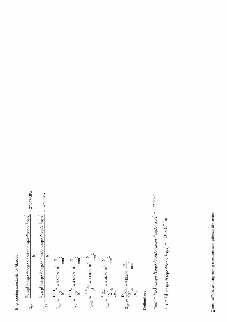
En

gin

ee

rin

g c

on

sta

nts

fo

r A

ba

qu

s

Ex

e

Ex

.ssp

hc.

ssp

At f

.top

A,

t f.b

otA

,

t c.s

spA

,

αss

pA

,

f ssp

A,

()

h2

7.0

67

GP

a⋅

=:=

Eye

Ey.s

sphc.

ssp

At f

.top

A,

t f.b

otA

,

t c.s

spA

,

αss

pA

,

f ssp

A,

()

h1

4.6

8G

Pa

⋅=

:=

Ex

b

12

Dx

⋅ h3

5.5

73

10

4×

N

mm

2⋅

=:=

Eyb

12

Dy

⋅ h3

4.6

17

10

4×

N

mm

2⋅

=:=

Gx

y.1

6D

xy

⋅ h3

1.6

02

10

4×

N

mm

2⋅

=:=

Gx

z

DQ

x1

5 6

h

⋅

4.4

69

10

3×

N

mm

2⋅

=:=

Gyz

DQ

y1

5 6

h

⋅

64

2.6

04

N

mm

2⋅

=:=

De

fle

ctio

ns

wto

t1w

tot

hc.

ssp

At f

.top

A,

t f.b

otA

,

t c.s

spA

,

αss

pA

,

f ssp

A,

()

6.7

21

8m

m⋅

=:=

δI.

1δI

hc.

ssp

At f

.top

A,

αss

pA

,

f ssp

A,

()

4.9

31

10

4−

×m

=:=

Are

a, st

iffn

ess

and e

ngin

eering c

onst

ants

with o

ptim

ised d

imensi

ons

Com

pariso

n a

nd U

tiliz

ation f

act

ors

Are

a p

er

un

it w

idth

Ass

pA

Asl

bH

K.f

.top

−

Asl

bH

K.f

.to

p

3.7

36

10

3−

×%

⋅=

Mo

me

nt o

f in

ert

ia p

er

un

it w

idth

I xI H

K.o

rth

o.x

− I HK

.ort

ho.x

59

.17

3−

%⋅

=

I yI H

K.o

rth

o.y

− I HK

.ort

ho.y

6.5

87

10

4×

%⋅

=

Axia

l S

tiff

ne

ss

Ex

Eort

ho.x

− Eort

ho.x

3.7

36

10

3−

×%

⋅=

Ey

Eort

ho.y

− Eort

ho.y

2.8

5−

%⋅

=

Be

nd

ing

Stiff

ne

ss

Dx

DH

K.o

rth

o.x

− DH

K.o

rth

o.x

59

.17

3−

%⋅

=

Dy

DH

K.o

rth

o.y

− DH

K.o

rth

o.y

6.0

95

10

4×

%⋅

=

To

rsio

na

l S

tiff

ne

ss

Dx

yT

HK

.ort

ho.x

y−

TH

K.o

rth

o.x

y

89

7.3

95

%⋅

=

Tra

nsve

rsa

l sh

ea

r stiff

ne

ss

DQ

x1

DH

K.o

rth

o.Q

x−

DH

K.o

rth

o.Q

x

40

9.7

%⋅

=

Glo

ba

l d

efl

ectio

n

wto

t1δm

ax.o

rth

o−

δm

ax.o

rth

o

27

.76

7%

⋅=

Lo

ca

l d

efl

ectio

n

δI.

1δlo

cal.

max

−

δlo

cal.

max

40

.08

4%

⋅=

Com

pariso

n a

nd U

tiliz

ation f

act

ors

Verifica

tion w

ith A

baqus

By c

alc

ula

tin

g th

e d

efl

ectio

n in

Ab

aq

us f

or

a s

imp

le s

up

po

rte

d e

qu

iva

len

t la

min

a p

late

with

th

e s

am

e c

on

sta

nts

:

δsi

mp

le.s

up

6.7

1m

m:=

De

fle

ctio

n in

th

e s

imp

le s

up

po

rte

d p

late

δsi

mp

le.s

up

wto

t1−

wto

t1

0.1

76

−%

⋅=

So

, it is c

lea

r th

at th

e o

ptim

iza

tio

n r

ou

tin

e c

orr

esp

on

ds r

ea

lly w

ell w

ith

th

e F

EM

mo

de

l.

Ho

we

ve

r, it is

vis

ible

th

at th

e m

axim

um

de

fle

ctio

n is d

isp

laye

d in

a d

iffe

ren

t p

ositio

n a

nd

no

t in

th

e m

idd

le o

f th

e p

late

. T

ha

t is

du

e to

th

e s

eco

nd

tru

ck a

dd

ed

. T

ha

t p

oin

t h

as c

oo

rdin

ate

s(2

m,5

.4m

) w

ith

a m

axim

um

de

fle

ctio

n 7

.35

mm

an

d it is

go

ing

to

be

use

d f

or

the

fo

llo

win

g a

na

lyse

s.

Verifica

tion w

ith A

baqus

CHALMERS Civil and Environmental Engineering, Master’s Thesis BOMX02-16-21

10 Appendix B

Cro

ss -

Sect

ion C

lass

ific

ation o

f th

e t

op p

late

of

Hoga K

ust

en B

ridge

Pa

rt o

f th

e c

om

pre

ssio

n f

lan

ge

be

twe

en

th

e w

eb

s o

f th

e r

ib

l HK

.rib

.top

.f.t

op

2t H

K.r

ib.t

op

2⋅

−

t HK

.f.t

op

24

.85

=

l HK

.rib

.top

.f.t

op

2t H

K.r

ib.t

op

2⋅

−

t HK

.f.t

op

33ε

⋅<

1=

Pla

te in

Cla

ss 1

Pa

rt o

f th

e c

om

pre

ssio

n f

lan

ge

ou

tsid

e th

e w

eb

s o

f th

e r

ib

bH

K.f

.top

l HK

.rib

.top

.f.t

op

−2

t HK

.rib

.top

2⋅

−

t HK

.f.t

op

23

.81

7=

bH

K.f

.top

l HK

.rib

.top

.f.t

op

−2

t HK

.rib

.top

2⋅

−

t HK

.f.t

op

33ε

⋅<

1=

Pla

te in

Cla

ss 1

Pa

rt o

f th

e c

om

pre

ssio

n f

lan

ge

in

th

e e

nd

of

the

pla

tes

l HK

.f.t

op

.en

d

t HK

.rib

.bot

2−

t HK

.f.t

op

16

.57

3=

l HK

.f.t

op

.en

d

t HK

.f.t

op

33ε

<1

=P

art

in

cla

ss 1

Bo

tto

m f

lan

ge

of

rib

l HK

.rib

.top

.f.b

ot

2t H

K.r

ib.t

op

2⋅

−

t HK

.rib

.top

18

.53

8=

l HK

.rib

.top

.f.b

ot

2t H

K.r

ib.t

op

2⋅

−

t HK

.rib

.top

33ε

⋅<

1=

Pa

rt in

cla

ss 1

We

bs o

f th

e to

p r

ibs

l HK

.rib

.top

.web

t HK

.f.t

op

2−

t HK

.rib

.top

2−

t HK

.rib

.top

37

.88

8=

l HK

.rib

.top

.web

t HK

.f.t

op

2−

t HK

.rib

.top

2−

t HK

.rib

.top

42ε

⋅<

0=

Pa

rt in

cla

ss 4

Cro

ss -

Sect

ion C

lass

ific

ation o

f th

e t

op p

late

of

Hoga K

ust

en B

ridge

Calc

ula

tion o

f eff

ect

ive a

rea o

f th

e t

op p

late

of

Hoga K

ust

en B

ridge

The s

olu

tion is a

ccord

ing t

o E

uro

code E

N_1993-1

-5

σH

K.r

ib.t

op

.f.b

ot

hb

ox

zn

a−

hH

K.r

ib.t

op

−

hb

ox

zn

a−

f y⋅

:=

σH

K.r

ib.t

op

.f.b

ot

28

0.9

54

MP

a⋅

=S

tresses in t

he b

ott

om

fla

nge o

f th

e t

op r

ibs

ψ1

σH

K.r

ib.t

op

.f.b

ot

f y

0.7

91

=:=

0ψ

1≤

1≤

1=

κσ

8.2

1.0

5ψ

1+

()

4.4

53

=:=

Bucklin

g f

acto

r κ.σ

for

uniform

com

pre

ssio

n

The w

ebs o

f th

e longitudin

al stiff

eners

are

in c

lass 4

σcr

κσ

ES

35

5Nπ

2⋅

12

1ν

2−

()

⋅

l HK

.rib

.to

p.w

eb

t HK

.rib

.to

p

2

⋅

⋅5

51

.77

6M

Pa

⋅=

:=E

lastic c

ritical pla

te b

ucklin

g s

tress o

f th

e e

quiv

ale

nt

ort

hotr

opic

pla

te f

or

the w

ebs

of

the t

op r

ibs

λp

f y

σcr

0.8

02

=:=

λp

0.6

73

>1

=P

late

sle

ndern

ess

ρλ

p0

.05

53

ψ1

+(

)⋅

−

λp

20

.92

3=

:=R

eduction f

acto

r ρ

l HK

.rib

.to

p.w

eb.e

ffρ

l HK

.rib

.to

p.w

eb

t HK

.f.t

op

2−

t HK

.rib

.to

p

2−

⋅

0.2

8m

=:=

Eff

ective length

of

the w

ebs in t

op r

ibs

hH

K.r

ib.t

op

.eff

ρh

HK

.rib

.to

p

t HK

.f.t

op

2−

t HK

.rib

.to

p

2−

⋅

0.2

71

m=

:=E

ffective v

ert

ical heig

ht

of

the w

ebs in t

op r

ibs

l HK

.rib

.to

p.w

eb.e

ff1

2

5ψ

1−

l HK

.rib

.to

p.w

eb.e

ff⋅

0.1

33

m=

:=Length

of

the t

op e

ffective p

art

of

the w

ebs

l HK

.rib

.to

p.w

eb.e

ff2

l HK

.rib

.to

p.w

eb.e

ffl H

K.r

ib.t

op

.web

.eff

1−

0.1

47

m⋅

=:=

Length

of

the b

ott

om

eff

ective p

art

of

the w

ebs

l HK

.rib

.to

p.w

eb.e

ff.n

ol H

K.r

ib.t

op

.web

l HK

.rib

.to

p.w

eb.e

ff1

−l H

K.r

ib.t

op

.web

.eff

2−

t HK

.f.t

op

2−

t HK

.rib

.to

p

2−

:=

l HK

.rib

.to

p.w

eb.e

ff.n

o0

.02

3m

=Length

of

the n

on e

ffective p

art

of

the w

ebs

hH

K.r

ib.t

op

.eff

12

5ψ

1−

hH

K.r

ib.t

op

.eff

⋅0

.12

9m

=:=

Heig

ht

of

the t

op e

ffective p

art

of

the w

ebs

hH

K.r

ib.t

op

.eff

2h

HK

.rib

.to

p.e

ffh

HK

.rib

.to

p.e

ff1

−0

.14

2m

=:=

Heig

ht

of

the b

ott

om

eff

ective p

art

of

the w

ebs

hH

K.r

ib.t

op

.eff

.no

hH

K.r

ib.t

op

hH

K.r

ib.t

op

.eff

1−

hH

K.r

ib.t

op

.eff

2−

t HK

.f.t

op

2−

t HK

.rib

.to

p

2−

:=

hH

K.r

ib.t

op

.eff

.no

0.0

23

m=

Heig

ht

of

the n

on e

ffective p

art

of

the w

ebs

Tota

l and e

ffective a

rea o

f lo

ngitudin

al stiff

eners

Asl

AH

K.u

nit

.ort

ho

.x1

.34

61

04

×m

m2

⋅=

:=

Asl

.eff

bH

K.f

.to

pt H

K.f

.to

p⋅

t HK

.rib

.to

p2

l HK

.rib

.to

p.w

eb.e

ff⋅

l HK

.rib

.to

p.f

.bo

t+

()

⋅+

1.2

92

10

4×

mm

2⋅

=:=

Calc

ula

tion o

f eff

ect

ive a

rea o

f th

e t

op p

late

of

Hoga K

ust

en B

ridge

Mom

ent

and a

xia

l lo

ad c

arr

yin

g c

apaci

ty o

f th

e t

op p

late

of

Hoga K

ust

en B

ridge

Co

lum

n-l

ike

bu

cklin

g b

eh

avio

ur

I sl

I HK

.un

it.o

rth

o.x

1.7

14

10

4−

×m

4=

:=

Mo

me

nt o

f in

ert

ia o

f e

ach

to

p r

ib

βA

c

Asl

.eff

Asl

0.9

6=

:=

σcr

.sl

π2

ES

35

5N

⋅I s

l⋅

Asl

l lon

g.s

tif2

⋅

1.6

49

10

3×

MP

a⋅

=:=

Ela

stic c

ritica

l co

lum

n b

ucklin

g s

tre

ss f

or

a s

tiff

en

ed

pla

te

λc

βA

cf y

⋅

σcr

.sl

0.4

55

=:=

Re

lative

co

lum

n s

len

de

rne

ss

iI s

l

Asl

11

2.8

36

mm

⋅=

:=

em

axz H

K.f

.top

z c,

z HK

.rib

.web

,

()

21

9.1

87

mm

⋅=

:=

La

rge

st d

ista

nce

fro

m th

e r

esp

ective

ce

ntr

oid

s o

f th

e p

late

fro

m th

e N

A

α0

.34

:=

Fo

r clo

se

d s

tiff

en

ers

αe

α0

.09

i e

+0

.51

5=

:=

Co

lum

n typ

e b

eh

avio

ur

Φ0

.51

αeλ

c0

.2−

()

⋅+

λc2

+

⋅

0.6

69

=:=

χc

1

ΦΦ

2λ

c2−

+

0.8

62

=:=

ρc

χc

0.8

62

=:=

Re

du

ctio

n f

acto

r ρ

fo

r th

e c

olu

mn

-lik

e b

ucklin

g

Pla

te-l

ike

bu

cklin

g u

sin

g e

qu

iva

len

t o

rth

otr

op

ic p

late

(h

alf

of

the

to

p p

late

is u

se

d f

or

the

ca

lcu

latio

ns)

α2

l lon

g.s

tif

l HK

.f.t

op

2

0.4

35

=:=

α2

0.5

>0

=L

en

gth

to

wid

th r

atio

of

the

to

p p

late

Alth

ou

gh

α.2

is n

ot b

igg

er

tha

n 0

.5 w

hic

h is th

e lim

it v

alu

e, h

an

d c

alc

ula

tio

ns a

cco

rdin

g to

An

ne

x A

are

go

ing

to

be

do

ne

, a

nd

th

en

a

re c

om

pa

red

with

EB

Pla

te p

rog

ram

re

su

lts, in

ord

er

to p

rovid

a m

ore

accu

rate

va

lue

.

ψp

lψ

1:=

ψp

l0

.5>

1=

I p

bH

K.f

.top

t HK

.f.t

op

3⋅

12

1ν

2−

()

⋅

9.4

95

10

4×

mm

4⋅

=:=

Se

co

nd

mo

me

nt o

f a

rea

fo

r b

en

din

g o

f th

e p

late

Ap

bH

K.f

.top

t HK

.f.t

op

⋅7

.21

03

−×

m2

=:=

Are

a o

f th

e p

late

γ2

I sl

I p

1.8

05

10

3×

=:=

Asl

.rib

6.2

61

03

−×

m2

=S

um

of

the

gro

ss a

rea

s o

f th

e in

div

idu

al lo

ng

itu

din

al stiff

en

ers

δ2

Asl

.rib

Ap

0.8

69

=:=

κσρ

21

α2

2+

2

γ2

+1

−

α2

2ψ

pl

1+

()

⋅1

δ2

+(

)⋅

α2

4γ

2≤

if

41

γ2

+(

)⋅

ψp

l1

+(

)1

δ2

+(

)α

24γ

2>

if

:=

Acco

rdin

g to

An

ne

x A

, E

uro

co

de

s 1

99

3-1

-5

κσρ

5.7

07

10

3×

=

As th

e A

nn

ex A

fo

r E

uro

co

de

ca

n n

ot b

e a

pp

lie

d, E

BP

late

pro

gra

mm

e is g

oin

g to

be

use

d f

or

the

ca

lcu

latio

n o

f th

e e

lastic c

ritica

l str

ess.

σcr

.p1

79

5.1

9M

Pa

:=

Ela

stic c

ritica

l str

ess f

or

the

pla

te-l

ike

bu

cklin

g

AH

K.c

om

p.f

AH

K.f

.top

AH

K.n

.rib

.top

+0

.40

9m

2=

:=

To

tal a

rea

of

the

co

mp

ressiv

e f

lan

ge

AH

K.r

ib.t

op

.eff

t HK

.rib

.top

2l H

K.r

ib.t

op

.web

.eff

⋅l H

K.r

ib.t

op

.f.b

ot

+(

)⋅

:=

AH

K.r

ib.t

op

.eff

5.7

25

10

3×

mm

2⋅

=E

ffe

ctive

are

a o

f e

ach

to

p r

ib

AH

K.n

.rib

.top

.eff

nH

K.r

ib.t

op

AH

K.r

ib.t

op

.eff

⋅0

.17

2m

2=

:=

To

tal e

ffe

ctive

are

a o

f th

e to

p r

ibs

AH

K.c

om

p.f

.eff

AH

K.f

.top

AH

K.n

.rib

.top

.eff

+0

.39

3m

2=

:=

To

tal e

ffe

ctive

are

a o

f th

e c

om

pre

ssiv

e f

lan

ge

βA

pl

AH

K.c

om

p.f

.eff

AH

K.c

om

p.f

0.9

61

=:=

0

λp

l

βA

pl

f y⋅

σcr

.p

0.4

36

=:=

Re

lative

pla

te s

len

de

rne

ss

ρp

l

λp

l0

.05

53

ψp

l+

()

−

λp

l2λ

pl

0.6

73

≥if

1oth

erw

ise

:=

ρp

l1

=ρ

pl

1≤

1=

Re

du

ctio

n f

acto

r ρ

fo

r th

e p

late

-lik

e b

ucklin

g

ξσ

cr.p

σcr

.sl

1−

0.0

88

=:=

ρc.

new

ρp

lχ

c−

()ξ

⋅2

ξ−

()

⋅χ

c+

:=

ρc.

new

0.8

86

=N

ew

re

du

ctio

n f

acto

r ρ

.c a

fte

r th

e in

tera

ctio

n b

etw

ee

n c

olu

mn

-lik

e a

nd

pla

te-l

ike

bu

cklin

g

Mo

me

nt C

ap

acity o

f th

e C

om

pre

ssiv

e F

lan

ge

Ne

w n

eu

tra

l a

xis

of

ea

ch

to

p r

ib (

dis

tan

ce

fro

m th

e c

en

tre

of

the

bo

tto

m f

lan

ge

of

the

rib

)

z c.n

ew

2l H

K.r

ib.t

op

.web

.eff

1t H

K.r

ib.t

op

⋅hH

K.r

ib.t

op

t HK

.f.t

op

2−

hH

K.r

ib.t

op

.eff

1

2−

⋅

l HK

.rib

.top

.web

.eff

2t H

K.r

ib.t

op

⋅

t HK

.rib

.top

2

hH

K.r

ib.t

op

.eff

2

2+

⋅

+

...

bH

K.f

.top

t HK

.f.t

op

⋅hH

K.r

ib.t

op

⋅+

Asl

.eff

:=

z c.n

ew0

.22

1m

=

z HK

.f.t

op

.new

hH

K.r

ib.t

op

z c.n

ew−

0.0

83

m=

:=

Dis

tan

ce

be

twe

en

th

e u

pp

er

pla

te a

nd

th

e n

eu

tra

l a

xis

of

the

rib

Mo

me

nt o

f In

ert

ia

I eff

1

bH

K.f

.top

t HK

.f.t

op

3⋅ 12

bH

K.f

.top

t HK

.f.t

op

⋅z H

K.f

.top

.new

2⋅

+

2t H

K.r

ib.t

op

hH

K.r

ib.t

op

.eff

13

⋅

12

t HK

.rib

.top

hH

K.r

ib.t

op

.eff

1⋅

z HK

.f.t

op

.new

hH

K.r

ib.t

op

.eff

1

2−

t HK

.f.t

op

2−

2

⋅+

...

+

...

:=

I eff

15

.23

41

07

×m

m4

⋅=

I eff

2

l HK

.rib

.top

.f.b

ot

t HK

.rib

.top

3⋅

12

l HK

.rib

.top

.f.b

ot

t HK

.rib

.top

⋅z c

.new

2⋅

+

2t H

K.r

ib.t

op

hH

K.r

ib.t

op

.eff

23

⋅

12

t HK

.rib

.top

hH

K.r

ib.t

op

.eff

2⋅

z c.n

ew

hH

K.r

ib.t

op

.eff

2

2−

t HK

.rib

.top

2−

2

⋅+

...

+

...

:=

I eff

21

.13

91

08

×m

m4

⋅=

I eff

I eff

1I e

ff2

+1

.66

21

08

×m

m4

⋅=

:=

Eff

ective

mo

me

nt o

f in

ert

ia

Fir

st m

om

en

t o

f a

rea

Wover

I eff

z HK

.f.t

op

.new

2.0

13

10

6×

mm

3⋅

=:=

Wu

nd

er

I eff

z c.n

ew

7.5

06

10

5×

mm

3⋅

=:=

Du

e to

th

e p

ositio

n o

f th

e n

eu

tra

l a

xis

or

ea

ch

rib

, yie

ldin

g w

ill p

rob

ab

ly ta

ke

pla

ce

at th

e b

otto

m f

lan

ge

of

the

rib

s a

nd

th

ere

fore

th

e b

en

din

g m

om

en

t ca

pa

city is d

efi

ne

d b

y th

e c

orr

esp

on

din

g f

irm

om

en

t o

f a

rea

an

d s

tre

sse

s a

t th

at d

ep

th. H

ow

eve

r, th

e m

om

en

t ca

pa

city o

f th

e to

p p

art

will b

e a

lso

fo

un

d to

ve

rify

it.

De

sig

n m

om

en

t ca

pa

city

MR

d.u

nit

.1W

over

f y

γM

1

⋅7

14

.60

1kN

m⋅

⋅=

:=

MR

d.u

nit

.2W

un

der

f y

γM

1

⋅2

66

.47

7kN

m⋅

⋅=

:=

MR

d.u

nit

min

MR

d.u

nit

.1M

Rd

.un

it.2

,

()

26

6.4

77

kN

m⋅

⋅=

:=

De

sig

n m

om

en

t ca

pa

city p

er

un

it le

ng

th

MR

d

MR

d.u

nit

bH

K.f

.top

44

4.1

29

kN

m⋅ m

⋅=

:=

In d

efi

nin

g th

e d

esig

n m

om

en

t ca

pa

city th

e e

nd

pa

rts in

ed

ge

s a

re n

eg

lecte

d.

Axia

l lo

ad

ca

rryin

g c

ap

acity

Fo

r a

stiff

en

ed

pla

te p

an

el th

e e

ffe

ctive

are

a o

f th

e c

om

pre

ssio

n z

on

e is:

Ac,e

ff =

ρc A

c,e

ff,loc +

Σb

edge,e

ff t , w

he

re A

c,e

ff,loc =

Asl,eff +

Σρ

loc b

c,loc t

Ac.

eff

ρc.

new

nH

K.r

ib.t

op

⋅A

sl.e

ff⋅

2l H

K.f

.top

.en

dt H

K.f

.top

⋅+

0.3

48

m2

=:=

Eff

ective

are

a p

er

un

it w

idth

Ac.

eff.

un

it

Ac.

eff

l HK

.f.t

op

:=

Ac.

eff.

un

it0

.01

9m

⋅=

To

tal lo

ad

ca

rryin

g c

ap

acity o

f th

e to

p p

late

NR

d.t

ot

Ac.

eff

f y

γM

1

⋅1

.23

61

05

×kN

⋅=

:=

Lo

ad

ca

rryin

g c

ap

acity p

er

un

it le

ng

th

NR

d

NR

d.t

ot

l HK

.f.t

op

6.7

18

10

3×

kN m

⋅=

:=

Mom

ent

and a

xia

l lo

ad c

arr

yin

g c

apaci

ty o

f th

e t

op p

late

of

Hoga K

ust

en B

ridge

Bendin

g m

om

ents

and u

tiliz

ation f

act

ors

in H

öga K

ust

en

ME

d1

29

kN

m m⋅

:=

uM

ME

d

MR

d

0.2

9=

:=

Bendin

g m

om

ents

and u

tiliz

ation f

act

ors

in H

öga K

ust

en

Are

as

of

the t

op S

SE

Ato

t.ss

pA

Ato

t.ss

phc.

ssp

At f

.top

A,

t f.b

otA

,

t c.s

spA

,

αss

pA

,

f ssp

A,

()

3.6

53

10

3×

mm

2⋅

=:=

Are

a o

f th

e r

ep

ea

ted

pa

rt o

f th

e S

SE

Ass

pA

0.0

2m

=A

rea

of

the

to

p S

SE

pe

r u

nit w

idth

Af.

top

.ssp

AA

ssp

Al H

K.f

.top

⋅0

.37

4m

2=

:=

To

tal a

rea

of

the

to

p S

SE

Ne

w to

tal a

rea

of

the

cro

ss-s

ectio

n

AH

K.t

ot.

ssp

Af.

top

.ssp

AA

HK

.web

.top

+A

HK

.n.s

id.s

tif

+A

HK

.sid

.pl

+A

HK

.web

.bot.

in+

AH

K.f

.bot

+A

HK

.n.r

ib.b

ot.

in+

AH

K.n

.rib

.bot

+:=

AH

K.t

ot.

ssp

0.8

54

m2

=To

tal a

rea

of

the

bo

x c

ross-s

ectio

n w

ith

th

e n

ew

SS

E

Are

as

of

the t

op S

SE

Gra

vity c

entr

es

of

SSE

Gra

vity c

en

tre

of

the

to

p S

SE

(d

ista

nce

fro

m th

e c

en

tre

lin

e o

f th

e to

p f

lan

ge

)

z na.

ssp

Az n

a.ss

phc.

ssp

At f

.top

A,

t f.b

otA

,

t c.s

spA

,

αss

pA

,

f ssp

A,

()

0.0

74

m=

:=

yf.

top

.ssp

A3

.81

5m

:=

Co

un

ted

fro

m th

e A

uto

ca

d d

ue

to

in

clin

atio

n

Gra

vity c

en

tre

of

the

se

ctio

n (

dis

tan

ce

fro

m th

e b

otto

m f

lan

ge

)

z na.

new

Af.

top

.ssp

Ayf.

top

.ssp

A⋅

AH

K.w

eb.t

op

yH

K.w

eb.t

op

⋅+

AH

K.n

.sid

.sti

fyH

K.s

id.s

tif

⋅+

AH

K.s

id.p

lyH

K.s

id.p

l⋅

AH

K.w

eb.b

ot.

inyH

K.w

eb.b

ot.

in⋅

+A

HK

.n.r

ib.b

ot.

inyH

K.n

.rib

.bot.

in⋅

+A

HK

.n.r

ib.b

ot

yH

K.n

.rib

.bot

⋅+

+

...

AH

K.t

ot.

ssp

2.2

64

m=

:=

Gra

vity c

entr

es

of

SSE

Mom

ent

and a

xia

l lo

ad c

arr

yin

g c

apaci

ty o

f th

e t

op S

SE

With

th

e s

am

e w

ay a

s d

on

e f

or

the

ort

ho

tro

pic

de

ck, th

e s

tre

sse

s in

th

e b

otto

m f

lan

ge

of

the

SS

E a

re f

ou

nd

:

σH

K.s

sp.f

.bot

hb

ox

z na.

new

−hss

pA

−

hb

ox

z na.

new

−

f y⋅

:=

σH

K.s

sp.f

.bot

31

8.1

27

MP

a⋅

=S

tre

sse

s in

th

e b

otto

m f

lan

ge

of

the

SS

E

ψ1

.ssp

σH

K.s

sp.f

.bot

f y

0.8

96

=:=

0ψ

1.s

sp≤

1≤

1=

Th

e w

ho

le c

ross-s

ectio

n o

f th

e s

tee

l sa

nd

wic

h e

lem

en

t is

in

cla

ss 3

. S

o, th

e w

ho

le a

rea

is e

ffe

ctive

. F

or

fin

din

g th

e r

ed

uctio

n f

acto

r d

ue

to

bu

cklin

g o

ne

of

the

re

pe

ate

d p

art

s o

f th

e s

tee

lsa

nd

wic

h e

lem

en

t is

go

ing

to

be

use

d.

Co

lum

n-l

ike

bu

cklin

g b

eh

avio

ur

I sl.

ssp

I tot.

ssp

.xhc.

ssp

At f

.top

A,

t f.b

otA

,

t c.s

spA

,

αss

pA

,

f ssp

A,

()

1.5

65

10

5−

×m

4=

:=

Mo

me

nt o

f in

ert

ia o

f e

ach

to

p r

ib

Asl

.ssp

Ato

t.ss

phc.

ssp

At f

.top

A,

t f.b

otA

,

t c.s

spA

,

αss

pA

,

f ssp

A,

()

3.6

53

10

3−

×m

2=

:=

βA

c.ss

p1

:=

Th

e w

ho

le c

ross-s

ectio

n is in

cla

ss 3

or

hig

he

r

σcr

.sl.

ssp

π2

ES

35

5N

⋅I s

l.ss

p⋅

Asl

.ssp

l lon

g.s

tif2

⋅

55

5.0

63

MP

a⋅

=:=

Ela

stic c

ritica

l co

lum

n b

ucklin

g s

tre

ss f

or

a s

tiff

en

ed

pla

te

λc.

ssp

βA

c.ss

pf y

⋅

σcr

.sl.

ssp

0.8

=:=

Re

lative

co

lum

n s

len

de

rne

ss

i ssp

I sl.

ssp

Asl

.ssp

65

.45

9m

m⋅

=:=

e ssp

max

z na.

ssp

Ahss

pA

z na.

ssp

A−

,

()

83

.69

9m

m⋅

=:=

La

rge

st d

ista

nce

fro

m th

e r

esp

ective

ce

ntr

oid

s o

f th

e p

late

fro

m th

e N

A

αss

p.

0.3

4:=

Fo

r clo

se

d s

tiff

en

ers

αe.

ssp

αss

p.

0.0

9

i ssp

ess

p

+0

.45

5=

:=

Co

lum

n typ

e b

eh

avio

ur

Φsp

p0

.51

αe.

sspλ

c.ss

p0

.2−

()

⋅+

λc.

ssp

2+

⋅0

.95

6=

:=

χc.

ssp

1

Φsp

pΦ

spp

2λ

c.ss

p2

−+

0.6

75

=:=

ρc.

ssp

χc.

ssp

0.6

75

=:=

Re

du

ctio

n f

acto

r ρ

fo

r th

e c

olu

mn

-lik

e b

ucklin

g

Pla

te-l

ike

bu

cklin

g u

sin

g e

qu

iva

len

t o

rth

otr

op

ic p

late

(h

alf

of

the

to

p p

late

is u

se

d f

or

the

ca

lcu

latio

ns)

ψp

l.ss

pψ

1.s

sp0

.89

6=

:=

Fo

r th

e s

tee

l sa

nd

wic

h e

lem

en

t, n

eith

er

the

Eu

roco

de

no

r th

e E

BP

late

so

ftw

are

co

uld

be

ap

plie

d d

ire

ctly.

Fo

llo

win

g J

ón

Pé

tur

Ind

rið

aso

n's

an

d V

éste

inn

Sig

mu

nd

sso

n's

Ma

ste

r T

he

sis

'Bu

cklin

ga

na

lysis

of

ort

ho

tro

pic

pla

tes',

an

eq

uiv

ale

nt p

late

co

uld

be

cre

ate

d th

at g

ive

s q

uite

clo

se

re

su

lts to

th

e s

tee

l sa

nd

wic

h e

lem

en

ts. F

or

de

cid

ing

th

e th

ickn

ess o

f th

e e

qu

iva

len

t p

late

, it is a

ssu

me

dth

at th

e to

tal b

en

din

g s

tiff

ne

ss o

f th

e n

ew

pla

te is e

qu

al w

ith

th

e b

en

din

g s

tiff

ne

ss o

f th

e s

tee

l sa

nd

wic

h e

lem

en

t in

th

e y

dir

ectio

n.

Dx

1.8

28

10

4×

kN

m⋅

⋅=

Dy

1.5

19

10

4×

kN

m⋅

⋅=

Deq

Dy

1.5

19

10

7×

Nm

⋅⋅

=:=

t eq

3

Deq

12

⋅1

ν2

−(

)⋅

ES

35

5N

0.0

92

m=

:=

βx

Dx

Deq

1−

0.2

03

=:=

ηx

Af.

top

.ssp

A

t eq

l HK

.f.t

op

⋅

1−

0.7

8−

=:=

Th

e, th

e s

oft

wa

re E

Bp

late

is u

se

d f

or

the

ne

w e

qu

iva

len

t p

late

.

σcr

.p.s

sp7

37

.75

MP

a:=

Ela

stic c

ritica

l str

ess f

or

the

pla

te-l

ike

bu

cklin

g

βA

pl.

ssp

βA

c.ss

p1

=:=

λp

l.ss

p

βA

pl.

ssp

f y⋅

σcr

.p.s

sp

0.6

94

=:=

Re

lative

pla

te s

len

de

rne

ss

ρp

l.ss

p

λp

l.ss

p0

.05

53

ψp

l.ss

p+

()

−

λp

l.ss

p2

λp

l.ss

p0

.67

3≥

if

1oth

erw

ise

:=

ρp

l.ss

p0

.99

6=

ρp

l.ss

p1

≤1

=R

ed

uctio

n f

acto

r ρ

fo

r th

e p

late

-lik

e b

ucklin

g

ξss

p

σcr

.p.s

sp

σcr

.sl.

ssp

1−

0.3

29

=:=

ρc.

new

.ssp

ρp

l.ss

pχ

c.ss

p−

()ξss

p⋅

2ξss

p−

()

⋅χ

c.ss

p+

:=

ρc.

new

.ssp

0.8

52

=N

ew

re

du

ctio

n f

acto

r ρ

.c a

fte

r th

e in

tera

ctio

n b

etw

ee

n c

olu

mn

-lik

e a

nd

pla

te-l

ike

bu

cklin

g

Mo

me

nt C

ap

acity o

f th

e C

om

pre

ssiv

e F

lan

ge

Fir

st m

om

en

t o

f a

rea

Wover

.ssp

I sl.

ssp

z na.

ssp

A

2.1

16

10

5×

mm

3⋅

=:=

Wu

nd

er.s

sp

I sl.

ssp

hss

pA

z na.

ssp

A−

1.8

71

05

×m

m3

⋅=

:=

Du

e to

th

e p

ositio

n o

f th

e n

eu

tra

l a

xis

or

ea

ch

rib

, yie

ldin

g w

ill p

rob

ab

ly ta

ke

pla

ce

at th

e b

otto

m f

lan

ge

of

the

rib

s a

nd

th

ere

fore

th

e b

en

din

g m

om

en

t ca

pa

city is d

efi

ne

d b

y th

e c

orr

esp

on

din

gfi

rst m

om

en

t o

f a

rea

an

d s

tre

sse

s a

t th

at d

ep

th. H

ow

eve

r, th

e m

om

en

t ca

pa

city o

f th

e to

p p

art

will b

e a

lso

fo

un

d to

ve

rify

it.

De

sig

n m

om

en

t ca

pa

city

MR

d.s

sp.1

Wover

.ssp

f y

γM

1

⋅7

5.1

08

kN

m⋅

⋅=

:=

MR

d.s

sp.2

Wu

nd

er.s

sp

f y

γM

1

⋅6

6.3

88

kN

m⋅

⋅=

:=

MR

d.s

sp.u

nit

min

MR

d.s

sp.1

MR

d.s

sp.2

,

()

66

.38

8kN

m⋅

⋅=

:=

De

sig

n m

om

en

t ca

pa

city p

er

un

it le

ng

th

MR

d.s

sp

MR

d.s

sp.u

nit

l ssp

A

36

9.1

25

kN

m⋅ m

⋅=

:=

In d

efi

nin

g th

e d

esig

n m

om

en

t ca

pa

city th

e e

nd

pa

rts in

ed

ge

s a

re n

eg

lecte

d.

Axia

l lo

ad

ca

rryin

g c

ap

acity

Eff

ective

are

a p

er

un

it w

idth

Ac.

eff.

ssp

ρc.

new

.ssp

Ass

pA

⋅0

.01

7m

=:=

Lo

ad

ca

rryin

g c

ap

acity p

er

un

it le

ng

th

NR

d.s

spA

c.ef

f.ss

p

f y

γM

1

⋅6

.14

21

03

×

kN m

⋅=

:=

Mom

ent

and a

xia

l lo

ad c

arr

yin

g c

apaci

ty o

f th

e t

op S

SE

Com

pariso

n a

nd U

tiliz

ation f

act

ors

MR

d.s

spM

Rd

−

MR

d

16

.88

8−

%⋅

=

NR

d.s

spN

Rd

−

NR

d

8.5

64

−%

⋅=

Com

pariso

n a

nd U

tiliz

ation f

act

ors

Are

as

of

the t

op S

SE

Ato

t.ss

pA

Ato

t.ss

phc.

ssp

At f

.top

A,

t f.b

otA

,

t c.s

spA

,

αss

pA

,

f ssp

A,

()

2.7

69

10

3×

mm

2⋅

=:=

Are

a o

f th

e r

ep

ea

ted

pa

rt o

f th

e S

SE

Ass

pA

0.0

17

m=

Are

a o

f th

e to

p S

SE

pe

r u

nit w

idth

Af.

top

.ssp

AA

ssp

Al H

K.f

.top

⋅0

.31

5m

2=

:=

To

tal a

rea

of

the

to

p S

SE

Ne

w to

tal a

rea

of

the

cro

ss-s

ectio

n

AH

K.t

ot.

ssp

Af.

top

.ssp

AA

HK

.web

.top

+A

HK

.n.s

id.s

tif

+A

HK

.sid

.pl

+A

HK

.web

.bot.

in+

AH

K.f

.bot

+A

HK

.n.r

ib.b

ot.

in+

AH

K.n

.rib

.bot

+:=

AH

K.t

ot.

ssp

0.7

95

m2

=To

tal a

rea

of

the

bo

x c

ross-s

ectio

n w

ith

th

e n

ew

SS

E

Are

as

of

the t

op S

SE

Gra

vity c

entr

es

of

SSE

Gra

vity c

en

tre

of

the

to

p S

SE

(d

ista

nce

fro

m th

e c

en

tre

lin

e o

f th

e to

p f

lan

ge

)

z na.

ssp

Az n

a.ss

phc.

ssp

At f

.top

A,

t f.b

otA

,

t c.s

spA

,

αss

pA

,

f ssp

A,

()

0.0

61

m=

:=

yf.

top

.ssp

A3

.81

5m

:=

Co

un

ted

fro

m th

e A

uto

ca

d d

ue

to

in

clin

atio

n

Gra

vity c

en

tre

of

the

se

ctio

n (

dis

tan

ce

fro

m th

e b

otto

m f

lan

ge

)

z na.

new

Af.

top

.ssp

Ayf.

top

.ssp

A⋅

AH

K.w

eb.t

op

yH

K.w

eb.t

op

⋅+

AH

K.n

.sid

.sti

fyH

K.s

id.s

tif

⋅+

AH

K.s

id.p

lyH

K.s

id.p

l⋅

AH

K.w

eb.b

ot.

inyH

K.w

eb.b

ot.

in⋅

+A

HK

.n.r

ib.b

ot.

inyH

K.n

.rib

.bot.

in⋅

+A

HK

.n.r

ib.b

ot

yH

K.n

.rib

.bot

⋅+

+

...

AH

K.t

ot.

ssp

2.1

49

m=

:=

Gra

vity c

entr

es

of

SSE

Mom

ent

and a

xia

l lo

ad c

arr

yin

g c

apaci

ty o

f th

e t

op S

SE

With

th

e s

am

e w

ay a

s d

on

e f

or

the

ort

ho

tro

pic

de

ck, th

e s

tre

sse

s in

th

e b

otto

m f

lan

ge

of

the

SS

E a

re f

ou

nd

:

σH

K.s

sp.f

.bot

hb

ox

z na.

new

−hss

pA

−

hb

ox

z na.

new

−

f y⋅

:=

σH

K.s

sp.f

.bot

32

6.7

39

MP

a⋅

=S

tre

sse

s in

th

e b

otto

m f

lan

ge

of

the

SS

E

ψ1

.ssp

σH

K.s

sp.f

.bot

f y

0.9

2=

:=

0ψ

1.s

sp≤

1≤

1=

Th

e w

ho

le c

ross-s

ectio

n o

f th

e s

tee

l sa

nd

wic

h e

lem

en

t is

in

cla

ss 3

. S

o, th

e w

ho

le a

rea

is e

ffe

ctive

. F

or

fin

din

g th

e r

ed

uctio

n f

acto

r d

ue

to

bu

cklin

g o

ne

of

the

re

pe

ate

d p

art

s o

f th

e s

tee

lsa

nd

wic

h e

lem

en

t is

go

ing

to

be

use

d.

Co

lum

n-l

ike

bu

cklin

g b

eh

avio

ur

I sl.

ssp

I tot.

ssp

.xhc.

ssp

At f

.top

A,

t f.b

otA

,

t c.s

spA

,

αss

pA

,

f ssp

A,

()

8.3

31

06

−×

m4

=:=

Mo

me

nt o

f in

ert

ia o

f e

ach

to

p r

ib

Asl

.ssp

Ato

t.ss

phc.

ssp

At f

.top

A,

t f.b

otA

,

t c.s

spA

,

αss

pA

,

f ssp

A,

()

2.7

69

10

3−

×m

2=

:=

βA

c.ss

p1

:=

Th

e w

ho

le c

ross-s

ectio

n is in

cla

ss 3

or

hig

he

r

Ac.

ssp

σcr

.sl.

ssp

π2

ES

35

5N

⋅I s

l.ss

p⋅

Asl

.ssp

l lon

g.s

tif2

⋅

38

9.6

24

MP

a⋅

=:=

Ela

stic c

ritica

l co

lum

n b

ucklin

g s

tre

ss f

or

a s

tiff

en

ed

pla

te

λc.

ssp

βA

c.ss

pf y

⋅

σcr

.sl.

ssp

0.9

55

=:=

Re

lative

co

lum

n s

len

de

rne

ss

i ssp

I sl.

ssp

Asl

.ssp

54

.84

3m

m⋅

=:=

e ssp

max

z na.

ssp

Ahss

pA

z na.

ssp

A−

,

()

69

.33

mm

⋅=

:=

La

rge

st d

ista

nce

fro

m th

e r

esp

ective

ce

ntr

oid

s o

f th

e p

late

fro

m th

e N

A

αss

p.

0.3

4:=

Fo

r clo

se

d s

tiff

en

ers

αe.

ssp

αss

p.

0.0

9

i ssp

ess

p

+0

.45

4=

:=

Co

lum

n typ

e b

eh

avio

ur

Φsp

p0

.51

αe.

sspλ

c.ss

p0

.2−

()

⋅+

λc.

ssp

2+

⋅1

.12

7=

:=

χc.

ssp

1

Φsp

pΦ

spp

2λ

c.ss

p2

−+

0.5

8=

:=

ρc.

ssp

χc.

ssp

0.5

8=

:=

Re

du

ctio

n f

acto

r ρ

fo

r th

e c

olu

mn

-lik

e b

ucklin

g

Pla

te-l

ike

bu

cklin

g u

sin

g e

qu

iva

len

t o

rth

otr

op

ic p

late

(h

alf

of

the

to

p p

late

is u

se

d f

or

the

ca

lcu

latio

ns)

ψp

l.ss

pψ

1.s

sp0

.92

=:=

Fo

r th

e s

tee

l sa

nd

wic

h e

lem

en

t, n

eith

er

the

Eu

roco

de

no

r th

e E

BP

late

so

ftw

are

co

uld

be

ap

plie

d d

ire

ctly.

Fo

llo

win

g J

ón

Pé

tur

Ind

rið

aso

n's

an

d V

éste

inn

Sig

mu

nd

sso

n's

Ma

ste

r T

he

sis

'Bu

cklin

g a

na

lysis

of

ort

ho

tro

pic

pla

tes',

an

eq

uiv

ale

nt p

late

co

uld

be

cre

ate

d th

at g

ive

s q

uite

clo

se

re

su

lts to

th

e s

tee

l sa

nd

wic

h e

lem

en

ts. F

or

de

cid

ing

th

e th

ickn

ess o

f th

e e

qu

iva

len

tp

late

, it is a

ssu

me

d th

at th

e to

tal b

en

din

g s

tiff

ne

ss o

f th

e n

ew

pla

te is e

qu

al w

ith

th

e b

en

din

g s

tiff

ne

ss o

f th

e s

tee

l sa

nd

wic

h e

lem

en

t in

th

e y

dir

ectio

n.

Dx

1.0

81

10

4×

kN

m⋅

⋅=

Dy

9.2

02

10

3×

kN

m⋅

⋅=

Deq

Dy

9.2

02

10

6×

Nm

⋅⋅

=:=

t eq

3

Deq

12

⋅1

ν2

−(

)⋅

ES

35

5N

0.0

78

m=

:=

βx

Dx

Deq

1−

0.1

75

=:=

ηx

Af.

top

.ssp

A

t eq

l HK

.f.t

op

⋅

1−

0.7

81

−=

:=

Th

e, th

e s

oft

wa

re E

Bp

late

is u

se

d f

or

the

ne

w e

qu

iva

len

t p

late

.

σcr

.p.s

sp1

07

3.4

5M

Pa

:=

Ela

stic c

ritica

l str

ess f

or

the

pla

te-l

ike

bu

cklin

g

βA

pl.

ssp

βA

c.ss

p1

=:=

λp

l.ss

p

βA

pl.

ssp

f y⋅

σcr

.p.s

sp

0.5

75

=:=

Re

lative

pla

te s

len

de

rne

ss

ρp

l.ss

p

λp

l.ss

p0

.05

53

ψp

l.ss

p+

()

−

λp

l.ss

p2

λp

l.ss

p0

.67

3≥

if

1oth

erw

ise

:=

ρp

l.ss

p1

=ρ

pl.

ssp

1≤

1=

Re

du

ctio

n f

acto

r ρ

fo

r th

e p

late

-lik

e b

ucklin

g

ξss

p

σcr

.p.s

sp

σcr

.sl.

ssp

1−

1.7

55

=:=

ρc.

new

.ssp

ρp

l.ss

pχ

c.ss

p−

()ξss

p⋅

2ξss

p−

()

⋅χ

c.ss

p+

:=

ρc.

new

.ssp

0.7

6=

Ne

w r

ed

uctio

n f

acto

r ρ

.c a

fte

r th

e in

tera

ctio

n b

etw

ee

n c

olu

mn

-lik

e a

nd

pla

te-l

ike

bu

cklin

g

Mo

me

nt C

ap

acity o

f th

e C

om

pre

ssiv

e F

lan

ge

Fir

st m

om

en

t o

f a

rea

Wover

.ssp

I sl.

ssp

z na.

ssp

A

1.3

73

10

5×

mm

3⋅

=:=

Wu

nd

er.s

sp

I sl.

ssp

hss

pA

z na.

ssp

A−

1.2

01

10

5×

mm

3⋅

=:=

Du

e to

th

e p

ositio

n o

f th

e n

eu

tra

l a

xis

or

ea

ch

rib

, yie

ldin

g w

ill p

rob

ab

ly ta

ke

pla

ce

at th

e b

otto

m f

lan

ge

of

the

rib

s a

nd

th

ere

fore

th

e b

en

din

g m

om

en

t ca

pa

city is d

efi

ne

d b

y th

eco

rre

sp

on

din

g f

irst m

om

en

t o

f a

rea

an

d s

tre

sse

s a

t th

at d

ep

th. H

ow

eve

r, th

e m

om

en

t ca

pa

city o

f th

e to

p p

art

will b

e a

lso

fo

un

d to

ve

rify

it.

De

sig

n m

om

en

t ca

pa

city

MR

d.s

sp.1

Wover

.ssp

f y

γM

1

⋅4

8.7

59

kN

m⋅

⋅=

:=

MR

d.s

sp.2

Wu

nd

er.s

sp

f y

γM

1

⋅4

2.6

51

kN

m⋅

⋅=

:=

MR

d.s

sp.u

nit

min

MR

d.s

sp.1

MR

d.s

sp.2

,

()

42

.65

1kN

m⋅

⋅=

:=

De

sig

n m

om

en

t ca

pa

city p

er

un

it le

ng

th

MR

d.s

sp

MR

d.s

sp.u

nit

l ssp

A

26

3.6

57

kN

m⋅ m

⋅=

:=

In d

efi

nin

g th

e d

esig

n m

om

en

t ca

pa

city th

e e

nd

pa

rts in

ed

ge

s a

re n

eg

lecte

d.

Axia

l lo

ad

ca

rryin

g c

ap

acity

Eff

ective

are

a p

er

un

it w

idth

Ac.

eff.

ssp

ρc.

new

.ssp

Ass

pA

⋅0

.01

3m

=:=

Lo

ad

ca

rryin

g c

ap

acity p

er

un

it le

ng

th

NR

d.s

spA

c.ef

f.ss

p

f y

γM

1

⋅4

.62

10

3×

kN m

⋅=

:=

Mom

ent

and a

xia

l lo

ad c

arr

yin

g c

apaci

ty o

f th

e t

op S

SE

Com

pariso

n a

nd U

tiliz

ation f

act

ors

MR

d.s

spM

Rd

−

MR

d

40

.63

5−

%⋅

=

NR

d.s

spN

Rd

−

NR

d

31

.22

2−

%⋅

=

Com

pariso

n a

nd U

tiliz

ation f

act

ors

Are

as

of

the t

op S

SE

Ato

t.ss

pA

Ato

t.ss

phc.

ssp

At f

.top

A,

t f.b

otA

,

t c.s

spA

,

αss

pA

,

f ssp

A,

()

4.5

88

10

3×

mm

2⋅

=:=

Are

a o

f th

e r

ep

ea

ted

pa

rt o

f th

e S

SE

Ass

pA

0.0

22

m=

Are

a o

f th

e to

p S

SE

pe

r u

nit w

idth

Af.

top

.ssp

AA

ssp

Al H

K.f

.top

⋅0

.41

3m

2=

:=

To

tal a

rea

of

the

to

p S

SE

Ne

w to

tal a

rea

of

the

cro

ss-s

ectio

n

AH

K.t

ot.

ssp

Af.

top

.ssp

AA

HK

.web

.top

+A

HK

.n.s

id.s

tif

+A

HK

.sid

.pl

+A

HK

.web

.bot.

in+

AH

K.f

.bot

+A

HK

.n.r

ib.b

ot.

in+

AH

K.n

.rib

.bot

+:=

AH

K.t

ot.

ssp

0.8

93

m2

=To

tal a

rea

of

the

bo

x c

ross-s

ectio

n w

ith

th

e n

ew

SS

E

Are

as

of

the t

op S

SE

Gra

vity c

entr

es

of

SSE

Gra

vity c

en

tre

of

the

to

p S

SE

(d

ista

nce

fro

m th

e c

en

tre

lin

e o

f th

e to

p f

lan

ge

)

z na.

ssp

Az n

a.ss

phc.

ssp

At f

.top

A,

t f.b

otA

,

t c.s

spA

,

αss

pA

,

f ssp

A,

()

0.0

81

m=

:=

yf.

top

.ssp

A3

.81

5m

:=

Co

un

ted

fro

m th

e A

uto

ca

d d

ue

to

in

clin

atio

n

Gra

vity c

en

tre

of

the

se

ctio

n (

dis

tan

ce

fro

m th

e b

otto

m f

lan

ge

)

z na.

new

Af.

top

.ssp

Ayf.

top

.ssp

A⋅

AH

K.w

eb.t

op

yH

K.w

eb.t

op

⋅+

AH

K.n

.sid

.sti

fyH

K.s

id.s

tif

⋅+

AH

K.s

id.p

lyH

K.s

id.p

l⋅

AH

K.w

eb.b

ot.

inyH

K.w

eb.b

ot.

in⋅

+A

HK

.n.r

ib.b

ot.

inyH

K.n

.rib

.bot.

in⋅

+A

HK

.n.r

ib.b

ot

yH

K.n

.rib

.bot

⋅+

+

...

AH

K.t

ot.

ssp

2.3

32

m=

:=

Gra

vity c

entr

es

of

SSE

Mom

ent

and a

xia

l lo

ad c

arr

yin

g c

apaci

ty o

f th

e t

op S

SE

With

th

e s

am

e w

ay a

s d

on

e f

or

the

ort

ho

tro

pic

de

ck, th

e s

tre

sse

s in

th

e b

otto

m f

lan

ge

of

the

SS

E a

re f

ou

nd

:

σH

K.s

sp.f

.bot

hb

ox

z na.

new

−hss

pA

−

hb

ox

z na.

new

−

f y⋅

:=

σH

K.s

sp.f

.bot

31

2.9

85

MP

a⋅

=S

tre

sse

s in

th

e b

otto

m f

lan

ge

of

the

SS

E

ψ1

.ssp

σH

K.s

sp.f

.bot

f y

0.8

82

=:=

0ψ

1.s

sp≤

1≤

1=

Th

e w

ho

le c

ross-s

ectio

n o

f th

e s

tee

l sa

nd

wic

h e

lem

en

t is

in

cla

ss 3

. S

o, th

e w

ho

le a

rea

is e

ffe

ctive

. F

or

fin

din

g th

e r

ed

uctio

n f

acto

r d

ue

to

bu

cklin

g o

ne

of

the

re

pe

ate

d p

art

s o

f th

e s

tee

lsa

nd

wic

h e

lem

en

t is

go

ing

to

be

use

d.

Co

lum

n-l

ike

bu

cklin

g b

eh

avio

ur

I sl.

ssp

I tot.

ssp

.xhc.

ssp

At f

.top

A,

t f.b

otA

,

t c.s

spA

,

αss

pA

,

f ssp

A,

()

2.3

61

05

−×

m4

=:=

Mo

me

nt o

f in

ert

ia o

f e

ach

to

p r

ib

Asl

.ssp

Ato

t.ss

phc.

ssp

At f

.top

A,

t f.b

otA

,

t c.s

spA

,

αss

pA

,

f ssp

A,

()

4.5

88

10

3−

×m

2=

:=

βA

c.ss

p1

:=

Th

e w

ho

le c

ross-s

ectio

n is in

cla

ss 3

or

hig

he

r

Ac.

ssp

σcr

.sl.

ssp

π2

ES

35

5N

⋅I s

l.ss

p⋅

Asl

.ssp

l lon

g.s

tif2

⋅

66

6.1

85

MP

a⋅

=:=

Ela

stic c

ritica

l co

lum

n b

ucklin

g s

tre

ss f

or

a s

tiff

en

ed

pla

te

λc.

ssp

βA

c.ss

pf y

⋅

σcr

.sl.

ssp

0.7

3=

:=

Re

lative

co

lum

n s

len

de

rne

ss

i ssp

I sl.

ssp

Asl

.ssp

71

.71

3m

m⋅

=:=

e ssp

max

z na.

ssp

Ahss

pA

z na.

ssp

A−

,

()

90

.87

5m

m⋅

=:=

La

rge

st d

ista

nce

fro

m th

e r

esp

ective

ce

ntr

oid

s o

f th

e p

late

fro

m th

e N

A

αss

p.

0.3

4:=

Fo

r clo

se

d s

tiff

en

ers

αe.

ssp

αss

p.

0.0

9

i ssp

ess

p

+0

.45

4=

:=

Co

lum

n typ

e b

eh

avio

ur

Φsp

p0

.51

αe.

sspλ

c.ss

p0

.2−

()

⋅+

λc.

ssp

2+

⋅0

.88

7=

:=

χc.

ssp

1

Φsp

pΦ

spp

2λ

c.ss

p2

−+

0.7

19

=:=

ρc.

ssp

χc.

ssp

0.7

19

=:=

Re

du

ctio

n f

acto

r ρ

fo

r th

e c

olu

mn

-lik

e b

ucklin

g

Pla

te-l

ike

bu

cklin

g u

sin

g e

qu

iva

len

t o

rth

otr

op

ic p

late

(h

alf

of

the

to

p p

late

is u

se

d f

or

the

ca

lcu

latio

ns)

ψp

l.ss

pψ

1.s

sp0

.88

2=

:=

Fo

r th

e s

tee

l sa

nd

wic

h e

lem

en

t, n

eith

er

the

Eu

roco

de

no

r th

e E

BP

late

so

ftw

are

co

uld

be

ap

plie

d d

ire

ctly.

Fo

llo

win

g J

ón

Pé

tur

Ind

rið

aso

n's

an

d V

éste

inn

Sig

mu

nd

sso

n's

Ma

ste

r T

he

sis

'Bu

cklin

g a

na

lysis

of

ort

ho

tro

pic

pla

tes',

an

eq

uiv

ale

nt p

late

co

uld

be

cre

ate

d th

at g

ive

s q

uite

clo

se

re

su

lts to

th

e s

tee

l sa

nd

wic

h e

lem

en

ts. F

or

de

cid

ing

th

e th

ickn

ess o

f th

e e

qu

iva

len

t p

late

,it is a

ssu

me

d th

at th

e to

tal b

en

din

g s

tiff

ne

ss o

f th

e n

ew

pla

te is e

qu

al w

ith

th

e b

en

din

g s

tiff

ne

ss o

f th

e s

tee

l sa

nd

wic

h e

lem

en

t in

th

e y

dir

ectio

n.

Dx

2.4

23

10

4×

kN

m⋅

⋅=

Dy

2.0

33

10

4×

kN

m⋅

⋅=

Deq

Dy

2.0

33

10

7×

Nm

⋅⋅

=:=

t eq

3

Deq

12

⋅1

ν2

−(

)⋅

ES

35

5N

0.1

02

m=

:=

βx

Dx

Deq

1−

0.1

92

=:=

ηx

Af.

top

.ssp

A

t eq

l HK

.f.t

op

⋅

1−

0.7

8−

=:=

Th

e, th

e s

oft

wa

re E

Bp

late

is u

se

d f

or

the

ne

w e

qu

iva

len

t p

late

.

σcr

.p.s

sp4

76

.41

MP

a:=

Ela

stic c

ritica

l str

ess f

or

the

pla

te-l

ike

bu

cklin

g

βA

pl.

ssp

βA

c.ss

p1

=:=

λp

l.ss

p

βA

pl.

ssp

f y⋅

σcr

.p.s

sp

0.8

63

=:=

Re

lative

pla

te s

len

de

rne

ss

ρp

l.ss

p

λp

l.ss

p0

.05

53

ψp

l.ss

p+

()

−

λp

l.ss

p2

λp

l.ss

p0

.67

3≥

if

1oth

erw

ise

:=

ρp

l.ss

p0

.87

2=

ρp

l.ss

p1

≤1

=R

ed

uctio

n f

acto

r ρ

fo

r th

e p

late

-lik

e b

ucklin

g

ξss

p

σcr

.p.s

sp

σcr

.sl.

ssp

1−

0.2

85

−=

:=

ρc.

new

.ssp

ρp

l.ss

pχ

c.ss

p−

()ξss

p⋅

2ξss

p−

()

⋅χ

c.ss

p+

:=

ρc.

new

.ssp

0.6

2=

Ne

w r

ed

uctio

n f

acto

r ρ

.c a

fte

r th

e in

tera

ctio

n b

etw

ee

n c

olu

mn

-lik

e a

nd

pla

te-l

ike

bu

cklin

g

Mo

me

nt C

ap

acity o

f th

e C

om

pre

ssiv

e F

lan

ge

Fir

st m

om

en

t o

f a

rea

Wover

.ssp

I sl.

ssp

z na.

ssp

A

2.9

22

10

5×

mm

3⋅

=:=

Wu

nd

er.s

sp

I sl.

ssp

hss

pA

z na.

ssp

A−

2.5

97

10

5×

mm

3⋅

=:=

Du

e to

th

e p

ositio

n o

f th

e n

eu

tra

l a

xis

or

ea

ch

rib

, yie

ldin

g w

ill p

rob

ab

ly ta

ke

pla

ce

at th

e b

otto

m f

lan

ge

of

the

rib

s a

nd

th

ere

fore

th

e b

en

din

g m

om

en

t ca

pa

city is d

efi

ne

d b

y th

e c

orr

esp

on

din

gfi

rst m

om

en

t o

f a

rea

an

d s

tre

sse

s a

t th

at d

ep

th. H

ow

eve

r, th

e m

om

en

t ca

pa

city o

f th

e to

p p

art

will b

e a

lso

fo

un

d to

ve

rify

it.

De

sig

n m

om

en

t ca

pa

city

MR

d.s

sp.1

Wover

.ssp

f y

γM

1

⋅1

03

.72

4kN

m⋅

⋅=

:=

MR

d.s

sp.2

Wu

nd

er.s

sp

f y

γM

1

⋅9

2.1

8kN

m⋅

⋅=

:=

MR

d.s

sp.u

nit

min

MR

d.s

sp.1

MR

d.s

sp.2

,

()

92

.18

kN

m⋅

⋅=

:=

De

sig

n m

om

en

t ca

pa

city p

er

un

it le

ng

th

MR

d.s

sp

MR

d.s

sp.u

nit

l ssp

A

45

0.6

96

kN

m⋅ m

⋅=

:=

In d

efi

nin

g th

e d

esig

n m

om

en

t ca

pa

city th

e e

nd

pa

rts in

ed

ge

s a

re n

eg

lecte

d.

Axia

l lo

ad

ca

rryin

g c

ap

acity

Eff

ective

are

a p

er

un

it w

idth

Ac.

eff.

ssp

ρc.

new

.ssp

Ass

pA

⋅0

.01

4m

=:=

Lo

ad

ca

rryin

g c

ap

acity p

er

un

it le

ng

th

NR

d.s

spA

c.ef

f.ss

p

f y

γM

1

⋅4

.93

71

03

×

kN m

⋅=

:=

Mom

ent

and a

xia

l lo

ad c

arr

yin

g c

apaci

ty o

f th

e t

op S

SE

Com

pariso

n a

nd U

tiliz

ation f

act

ors

MR

d.s

spM

Rd

−

MR

d

1.4

79

%⋅

=

NR

d.s

spN

Rd

−

NR

d

26

.50

4−

%⋅

=

Com

pariso

n a

nd U

tiliz

ation f

act

ors

steel-sandwich elements in long-span bridge applications

Documents