stats lecture 09 small samples

8/3/2019 Stats Lecture 09 Small Samples

http://slidepdf.com/reader/full/stats-lecture-09-small-samples 1/44

Inference From Small Samples

Quantitative Methods for EconomicsDr. Katherine SauerMetropolitan State College of Denver



Chapter Overview:

I. Normal Population, σ is known

II. The t -distribution (aka Student’s t -distribution)III. Difference Between Means from Small, Independent SamplesIV. The F-test for equality of two variancesV. Difference between Means, Paired Samples



I. Normal Population, σ is known

For n < 30:

When the population is Normal and the population standard deviationis known, then the sampling distribution for sample means is

n N x

,~

The confidence interval is

The Test Statistic is

x Z x 2 /

x

H x Z

0



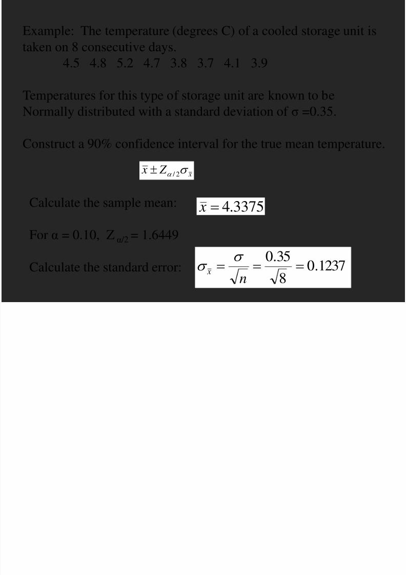
Example: The temperature (degrees C) of a cooled storage unit istaken on 8 consecutive days.

4.5 4.8 5.2 4.7 3.8 3.7 4.1 3.9

Temperatures for this type of storage unit are known to beNormally distributed with a standard deviation of σ =0.35.

Construct a 90% confidence interval for the true mean temperature.

3375.4 xCalculate the sample mean:

For α = 0.10, Z α /2 = 1.6449

Calculate the standard error:

x Z x 2 /

1237.0

8

35.0

n x



4.3375 + 1.6449(0.1237)4.3375 + 0.2035

4.1340 to 4.5410

We are 90% sure that the true population mean is in thisinterval.



Test the hypothesis that the mean temperature is 4 degrees.

H0: µ = 4H1: µ ≠ 4

For α = 0.10, α / 2 = 0.05 Z = 1.6449

µ= 4

Z = -1.6449

RejectH0

Accept H0

Z = 1.6449

RejectH0

Reject the null if Z > 1.6449 or Z < -1.6449

x

H x

x Z

0

n x

73.21237.0

43375.4 x Z

Z = 2.73

Reject the null and conclude that the

average temperature is not 4 degrees.



p-value = pr (Z > 2.73) + pr(Z < -2.73)= 0.0032 + 0.0032= 0.0064

There is only a 0.64% chance of selecting the given sample if the true mean is 4.



Often, we don’t know the population standard deviation.

We can no longer use the Z table.



II. The t -distribution (aka Student’s t -distribution)

Fun origin: A chemist at the Guinness brewery in Dublin inventedthe t-distribution in order to monitor quality in brewing, usingsmall samples from Normal populations with σ unknown.

If random samples of size n are selected from a Normal populationwith mean µ and σ unknown, then the distribution of sample meansis a t-distribution.

xn st x ,~ 1 n

ss

x

(n-1) refers to the degrees of freedom



The t-distribution is similar to the Normal distribution in severalways:

it is bell shapedit is symmetrical about the mean

is the number of standard errors between thesample mean and population mean x

s

xt



Ex: find the tailarea equal to5% when the

sample size is10.

10-1 =9 degreesof freedom

Tail area = 0.05

Critical t-valueis 1.8331



In large samples, when σ is unknown, we often use Z instead of t.

When samples are large, Z and t are close.

Statistical software always uses t when σ is unknown, even forlarge samples.



The confidence interval for a small sample from a Normalpopulation with unknown σ is

xn st x 2 / ,1

The test statistic for a small sample from a Normal populationwith unknown σ is

xs

xt



Example: The waiting time at an airline check in counter isknown to be Normally distributed. A random sample of 5passengers were interviewed. They reported the following waittimes: 15.5 21.2 12.6 18.4 22.9 minutes.Construct a 90% confidence interval for the average wait time.

Calculate the sample average wait time: 12.18 x

n

ss

xCalculate the standard error:

Remember todivide by n-1

for thevariance!!!

xi xi - mean (xi - mean)^2 mean 18.1215.5 -2.62 6.8644 variance 17.43721.2 3.08 9.4864 st dev 4.17576312.6 -5.52 30.470418.4 0.28 0.078422.9 4.78 22.8484

69.748 sum



8675.15

1758.4

n

ss x

xn st x 2 / ,1

Find the critical value for t :tn-1, α /2 = t 4, 0.05 = 2.1318

Construct the interval:

18.12 + (2.1318)(1.8675)18.12 + 3.981114.1389 to 22.1011

We are 90% confident that the average wait time is inthis range.



Example: Test the hypothesis that the average wait time is atmost 20 minutes.

1. State the null and alternative hypothesesH0: µ < 20H1: µ > 20

one-sided test, upper tail

2. Sketch the graph and identify the critical regionα =0.10 t 4, 0.1 = 1.5332

µ =20

t =1.5332

RejectH0

Accept H0 Accept H 0 if 1.5332 < t

Reject H 0 if t > 1.5332



3. Calculate t: x

s

xt

n

ss

x

8675.15

1758.4n

ss x 0067.18675.1

2012.18t

12.18 x

µ =20

t =1.5332

RejectH0

Accept H0

t = -1.0067

Accept H 0 because-1.0067 < 1.5332

Accept the null and validate the claim that at most the averagewait time is 20 minutes.



4. p-value is the area to the right of -1.0067

(rarely look up in t- distribution table… software)



Example: The temperature (degrees C) of a cooled storage unit istaken on 8 consecutive days.

4.5 4.8 5.2 4.7 3.8 3.7 4.1 3.9

At the 90% level, test the hypothesis that the mean temperature is4 degrees.

H0: µ = 4H1: µ ≠ 4



xi xi - mean (xi - mean)^2 mean 4.33754.5 0.1625 0.0264 variance 0.2941074.8 0.4625 0.2139 st dev 0.542316

5.2 0.8625 0.74394.7 0.3625 0.13143.8 -0.5375 0.28893.7 -0.6375 0.40644.1 -0.2375 0.05643.9 -0.4375 0.1914

2.0588 sum

Let’s verify the output:

1917.08

542316.0

n

ss x



xn st x 2 / ,1 t 7, 0.05 = 1.8946

4.3375 + (1.8946)(0.19174)4.3375 + 0.3633

3.9742 to 4.7008



xs

xt

76.1

19174.0

43375.4t

This is a two-tail test.

- 1.8946 < 1.76 < 1.8946

Accept the null.

If we had rejected the null, the p-value would have told us thelevel of significance.



III. Difference Between Means from Small, Independent Samples

Example: Promoters of e-learning software design a test foreffectiveness of an online course based on typing tutor software.Two groups are randomly selected. Group 1 consists of 10 subjectswho have completed a course that did not use supporting software.Group 2 consists of 8 subjects who used the online software.

The typing speeds (wpm) are as follows.Group 1: 23, 35, 37, 12, 26, 60, 13, 24, 27, 53

Group 2: 56, 30, 55, 48, 35, 40, 33, 23

Construct a 90% confidence interval for the difference in meantyping speed between the two groups. Can you conclude that thosewho used the online software can type faster?



xi xi - mean ( xi - mean)^2 xi xi - mean ( xi - mean)^223 -8 64 56 16 25635 4 16 30 -10 10037 6 36 55 15 22512 -19 361 48 8 6426 -5 25 35 -5 2560 29 841 40 0 013 -18 324 33 -7 4924 -7 49 23 -17 28927 -4 16 sum 100853 22 484

sum 2216

mean 31 mean 40variance 246.2222 variance 144

st dev 15.69147 st dev 12

Group 1 Group 2



We’ll need to construct a pooled estimate of variance .

2

)1()1(

21

222

2112

nn

snsns

p

5.2012810

)12)(18()69147.15)(110( 222 ps

Use the pooled estimate of variance to find the standard error.

21

2 1121 nn

ss p x x

7333.68

1

10

15.201

21

x xs



Find the critical t value:degrees of freedom = n1 + n2 – 2

= 16

α / 2 = 0.05

t 16, 0.05 = 1.7459

Construct the interval:40 – 31 + 1.7459(6.7333)9 + 11.7557

-2.7557 to 20.7557The interval contains 0. We can conclude that thedifference between means is zero.

Typing speeds between the 2 groups are the same.



At the 95% level, test the hypotheses that the mean typing speed isfaster for those who used the software.

H0: µ 1 = µ 2H1: µ 1 > µ 2

one tailed test

α = 0.05

t 16, 0.05 = 1.7459

µ1 = µ2

Accept H0

t = 1.7459

RejectH0



t =1.3366

The test statistic is

21

2

2121

11

)()(

nns

x xt

p

3366.17333.6

)0()3140(t

µ1 = µ2

Accept H0

t = 1.7459

RejectH0

Accept the nullhypotheses that thetyping speed of both

groups is the same.



Assumptions made in solving this problem:1. independent samples2. random samples from Normal populations3. the variance is the same for both populations



IV. The F-test for equality of two variances

To figure out if two populations have similar variances, we will look at the sample variances.

If the ratio of the sample variances is close to 1, then the hypothesisthat the populations have equal variance is plausible.

The sampling distribution of is an F-distribution, when thesamples are independent and selected from Normal populationswith equal variances.

2

2

2

1

s

s



The F-distribution is not symmetrical and depends on thedegrees of freedom in each sample.

v1 = n1 – 1 v2 = n2 - 1



Ex: Suppose sample 1 has 10 observations and sample 2 has 8observations. Find the critical F-value for the 5% level.

v1 = 9 v2 = 7



If we wanted the 2.5% level, we’d need a different table.



Example: Using the data from the typing example, test whetherthe sample variances are equal at the 95% level.

H0: σ21 = σ22 H1: σ2

1 ≠ σ 22

this is a 2-tail test

α /2 = 0.025F: v1 = 10-1 = 9 v2 = 8-1 = 7

F = 4.82



Calculate the test statistic2

2

2

1

s

s

7099.1144

22.24622

21

ss

F = 1.7099

Accept the nullhypothesis andconclude that thepopulation variancesare equal.



Instead, test the hypothesis that the variance of population 1exceeds the variance of population 2.

H0: σ21 < σ22 H1: σ2

1 > σ22

this is a 1-tail test, upper tail

α= 0.05F: v1 = 10-1 = 9 v2 = 8-1 = 7

F = 3.69



Calculate the test statistic2

2

2

1

s

s

7099.1144

22.24622

21

ss

F = 1.7099

Accept the nullhypothesis andconclude thevariance of

population 1 is lessthan or equal to thevariance of population 2.



V. Difference between Means, Paired Samples

Paired t-tests are used when data consists of pairs of measurementson the same subjects.

ex: before and after



Example: The typing speeds for 7 people are recorded before andafter completing a course using typing tutor software.

Person Before After DifferenceJM 32 46 14AC 10 18 8TB 65 58 -7

AF 39 50 11AO 24 36 12PD 10 24 14FF 24 21 -3

Construct a 90% confidence interval for the difference betweenaverage typing speed before and after the course.

α /2 = 0.05degrees of freedom = 7-1 = 6

t 6, 0.05 = 1.9432



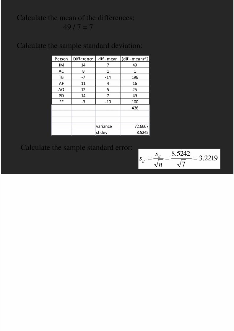
Calculate the mean of the differences:49 / 7 = 7

Calculate the sample standard deviation:

Person Difference dif - mean (dif - mean)^2JM 14 7 49AC 8 1 1TB -7 -14 196

AF 11 4 16AO 12 5 25PD 14 7 49FF -3 -10 100

436

variance 72.6667st dev 8.5245

Calculate the sample standard error:2219.3

7

5242.8

n

ss d

d



Construct the interval:

7 + 1.9432(3.2219)7 + 6.2608

0.7392 to 13.2608

We are 90% confident that the true difference in average typingspeeds is between 0.7392 words per minute and 13.2608 words

per minute.



Now at the 2.5% level, test the hypothesis that typing speeds have

increased after taking the course.

H0 : µ d < 0H1: µ d > 0

one sided test

α = 0.025

degrees of freedom = 6

t 6, 0.025 = 2.447



t =2.1726

µd = 0

Accept H0

t = 2.447

RejectH0

Calculate the test statistic:

sterror claim H estimate

t 0

1726.22219.3

07t

Accept the null hypothesis andconclude that typing speeds did

not improve during the course.



Concepts:t-distributionF-distribution

Skills:Construct confidence interval and perform hypothesis test formeans from small, independent samples

Perform an F-test

Construct confidence interval and perform hypothesis test for the

difference between means from small, independent samples

Construct confidence interval and perform hypothesis test for thedifference between paired means from small, independent samples

stats lecture 09 small samples

Documents