stats 8: introduction to biostatistics 24pt...
TRANSCRIPT
STATS 8: Introduction to Biostatistics
Estimation
Babak ShahbabaDepartment of Statistics, UCI

Parameter estimation
• We are interested in population mean and population variance,denoted as µ and σ2 respectively, of a random variable.
• These quantities are unknown in general.
• We refer to these unknown quantities as parameters.
• We discuss statistical methods for parameter estimation.
• Estimation refers to the process of guessing the unknownvalue of a parameter (e.g., population mean) using theobserved data.

Convention
• We use X1,X2, . . . ,Xn to denote n possible values of Xobtained from a sample randomly selected from thepopulation.
• We treat X1,X2, . . . ,Xn themselves as n random variablesbecause their values can change depending on which nindividuals we sample.
• We assume the samples are independent and identicallydistributed (IID).
• We use x1, x2, . . . , xn as the specific set of values we haveobserved in our sample.
• That is, x1 is the observed value for X1, x2 is the observedvalue X2, and so forth.

Point estimation vs. interval estimation
• Sometimes we only provide a single value as our estimate.
• This is called point estimation.
• We use µ̂ and σ̂2 to denote the point estimates for µ and σ2.
• Point estimates do not reflect our uncertainty.
• To address this issue, we can present our estimates in terms ofa range of possible values (as opposed to a single value).
• This is called interval estimation.

Estimating population mean
• Given n observed values, X1,X2, . . . ,Xn, from the population,we can estimate the population mean µ with the sample mean:
X̄ =
∑ni=1 Xi
n.
• In this case, we say that X̄ is an estimator for µ.
• The estimator itself is considered as a random variable since itvalue can change.
• We usually have only one sample of size n from thepopulation x1, x2, . . . , xn.
• Therefore, we only have one value for X̄ , which we denote x̄ :
x̄ =
∑ni=1 xin

Law of Large Numbers (LLN)
• The Law of Large Numbers (LLN) indicates that (undersome general conditions such as independence ofobservations) the sample mean converges to the populationmean (X̄n → µ) as the sample size n increases (n→∞).
• Informally, this means that the difference between the samplemean and the population mean tends to become smaller andsmaller as we increase the sample size.
• The Law of Large Numbers provides a theoretical justificationfor the use of sample mean as an estimator for the populationmean.
• The Law of Large Numbers is true regardless of the underlyingdistribution of the random variable.
Law of Large Numbers (LLN)
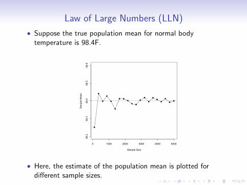
• Suppose the true population mean for normal bodytemperature is 98.4F.
0 1000 2000 3000 4000 5000
98.2
98.3
98.4
98.5
98.6
Sample Size
Sam
ple
Mea
n
• Here, the estimate of the population mean is plotted fordifferent sample sizes.

Estimating population variance
• Given n randomly sampled values X1,X2, . . . ,Xn from thepopulation and their corresponding sample mean X̄ , weestimate the population variance as follows:
S2 =
∑ni=1(Xi − X̄ )2
n − 1.
• The sample standard deviation S (i.e., square root of S2) isour estimator of the population standard deviation σ.
• We regard the estimator S2 as a random variable.
• In practice, we usually have one set of observed values,x1, x2, . . . , xn, and therefore, only one value for S2:
s2 =
∑ni=1(xi − x̄)2
n − 1.
Sampling distribution
• As mentioned above, estimators are themselves randomvariables.
• Probability distributions for estimators are called samplingdistributions.
• Here, we are mainly interested in the sampling distribution ofX̄ .

Sampling distribution
• We start by assuming that the random variable of interest, X ,has a normal N(µ, σ2) distribution.
• Further, we assume that the population variance σ2 is known,so the only parameter we want to estimate is µ.
• In this case,X̄ ∼ N
(µ, σ2/n
).
where n is the sample size.
Sampling distribution
80 100 120 140 160
0.00
00.
005
0.01
00.
015
0.02
00.
025
X
Den
sity
X
dens
ity
120 122 124 126 128 130
0.00
0.05
0.10
0.15
0.20
0.25
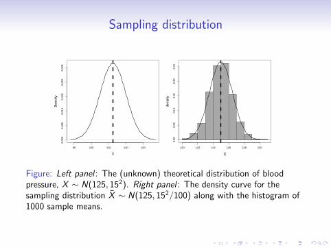
Figure: Left panel : The (unknown) theoretical distribution of bloodpressure, X ∼ N(125, 152). Right panel : The density curve for thesampling distribution X̄ ∼ N(125, 152/100) along with the histogram of1000 sample means.

Confidence intervals for the population mean
• It is common to express our point estimate along with itsstandard deviation to show how much the estimate could varyif different members of population were selected as oursample.
• Alternatively, we can use the point estimate and its standarddeviation to express our estimate as a range (interval) ofpossible values for the unknown parameter..

Confidence intervals for the population mean
• We know that X̄ ∼ N(µ, σ2/n).
• Suppose that σ2 = 152 and sample size is n = 100.
• Following the 68–95–99.7% rule, with 0.95 probability, thevalue of X̄ is within 2 standard deviations from its mean, µ,
µ− 2× 1.5 ≤ X̄ ≤ µ+ 2× 1.5.
• In other words, with probability 0.95,
µ− 3 ≤ X̄ ≤ µ+ 3.
Confidence intervals for the population mean
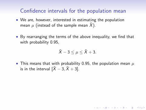
• We are, however, interested in estimating the populationmean µ (instead of the sample mean X̄ ).
• By rearranging the terms of the above inequality, we find thatwith probability 0.95,
X̄ − 3 ≤ µ ≤ X̄ + 3.
• This means that with probability 0.95, the population mean µis in the interval [X̄ − 3, X̄ + 3].

Confidence intervals for the population mean
• In reality, however, we usually have only one sample of nobservations, one sample mean x̄ , and one interval[x̄ − 3, x̄ + 3] for the population mean µ.
• For the blood pressure example, suppose that we have asample of n = 100 people and that the sample mean isx̄ = 123. Therefore, we have one interval as follows:
[123− 3, 123 + 3] = [120, 126].
• We refer to this interval as our 95% confidence interval forthe population mean µ.
• In general, when the population variance σ2 is known, the95% confidence interval for µ is obtained as follows:[
x̄ − 2× σ/√n, x̄ + 2× σ/
√n]

z critical value
• In general, for the given confidence level c, we use thestandard normal distribution to find the value whose uppertail probability is (1− c)/2.
−4 −2 0 2 4
0.0
0.1
0.2
0.3
0.4
Z
Den
sity
z
0.8

z critical value
• We refer to this value as the z-critical value for the confidencelevel of c .
• Then with the point estimate x̄ , the confidence interval forthe population mean at c confidence level is
[x̄ − zcrit × σ/√n, x̄ + zcrit × σ/
√n]
• We can use R or R-Commander to find zcrit .
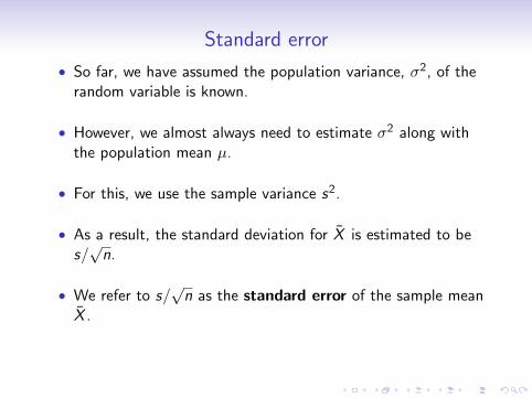
Standard error
• So far, we have assumed the population variance, σ2, of therandom variable is known.
• However, we almost always need to estimate σ2 along withthe population mean µ.
• For this, we use the sample variance s2.
• As a result, the standard deviation for X̄ is estimated to bes/√n.
• We refer to s/√n as the standard error of the sample mean
X̄ .

Confidence Interval When the Population Variance IsUnknown
• To find confidence intervals for the population mean when thepopulation variance is unknown, we follow similar steps asdescribed above, but
• instead of σ/√n we use SE = s/
√n,
• instead of zcrit based on the standard normal distribution, weuse tcrit obtained from a t-distribution with n − 1 degrees offreedom.
• The confidence interval for the population mean at cconfidence level is[
x̄ − tcrit × s/√n, x̄ + tcrit × s/
√n],

Central limit theorem
• So far, we have assumed that the random variable has normaldistribution, so the sampling distribution of X̄ is normal too.
• If the random variable is not normally distributed, thesampling distribution of X̄ can be considered as approximatelynormal using (under certain conditions) the central limittheorem (CLT):
If the random variable X has the populationmean µ and the population variance σ2, thenthe sampling distribution of X̄ is approximatelynormal with mean µ and variance σ2/n.
• Note that CLT is true regarding the underlying distribution ofX so we can use it for random variables with Bernoulli andBinomial distributions too.

Confidence Interval When for the Population Proportion
• For binary random variables, we use the sample proportion toestimate the population proportion as well as the populationvariance.
• Therefore, estimating the population variance does notintroduce an additional source of uncertainty to our analysis,so we do not need to use a t-distribution instead of thestandard normal distribution.
• For the population proportion, the confidence interval isobtained as follows:
[p − zcrit × SE , p + zcrit × SE ],
whereSE =
√p(1− p)/n.