statistics in practice: study design and application of

Statistics in Practice: Study Design and Application of Inferential Statistics – Interventional Research WEBPAGE 1 Randomization Techniques Case 1 The BNT162b2 messenger RNA (mRNA) COVID-19 vaccine was evaluated in a double-blind (subject and observer blinded), placebo-controlled, pivotal efficacy trial (Polack 2020) in which 43,548 subjects received either two doses of vaccine (21 days apart) or two doses of placebo. In this study, BNT162b2 was 95% effective in preventing COVID-19 (95% credible interval, 90.3–97.6). Safety data were available for around 38,000 subjects, with a median follow-up of 2 months at the time of Emergency Use Authorization by the FDA. Investigators sought to achieve at least 40% of study enrollment with adults older than 55 and later to include adolescents 12–15 years of age. Which one of the following strategies would be most appropriate to conduct this trial? A. Block randomization. B. Stratified randomization on the basis of age. (CORRECT) C. Cluster randomization. D. No randomization. WEBPAGE 2 Detailed Feedback Introduction This feature addresses elements of study design and conduct for interventional research and build on prior features in this series that have focused on inferential statistical tests for interventional research. Topics include randomization and blinding techniques, subgroup analyses, composite end points, early cessation of clinical trials, internal and external validity, sample size estimation, and measures of effect in clinical trials. These elements are key to data quality and analysis and require careful consideration when evaluating clinical trials. Randomization (randomly assigning subjects to treatment and control groups) helps eliminate selection bias and balance potential confounding variables evenly between groups (Hartung 2009). A randomized approach does not guarantee equal distribution of potential confounders, and a successful balance of confounders will depend on the number of study subjects and the randomization strategy used. Using simple strategies such as sequentially allocating subjects between treatment and control as subjects accrue or making assignments according to day of the week, clinic site, or provider are not truly random and can result in experimental groups that are not well balanced on the basis of potential confounders. For example, a simple, unrestricted randomization strategy such as assigning groups on the basis of a coin flip might not guarantee the even distribution of confounders (or even properly allotted numbers of subjects), particularly if the number of subjects is relatively small (Broglio 2018).

Block randomization (permuted block randomization) involves random assignments made in blocks, with each block containing the desired allocation proportions (Broglio 2018). For example, in a trial with two equally allocated groups (treatment “T” and placebo “P”) and a block size of four, two subjects in each block would be assigned to receive treatment and two to receive placebo; possible blocks would be TTPP, PPTT, TPTP, TPPT, PTTP, and PTPT (Broglio 2018; Hartung 2009). When a given block is filled, the next block would be started (Broglio 2018). A limitation to block randomization is that if treatment assignments are known to investigators or clinicians, they become predictable (i.e., the last treatment assignment can be predicted if the others are known) (Broglio 2018). Stratified randomization helps ensure equal distribution of known, measurable, confounding variables (that are considered associated with the outcome of interest) at the time of randomization (Broglio 2018). “Strata” are defined on the basis of the categories of confounding variables, and the stratification does not necessarily result in equal distribution of confounding variables that are unknown or unmeasured at the time of randomization. For example, in a study that stratifies on the basis of enrollment age (younger than 65, 65 and older) and diagnosis of hypertension (yes or no), there would be four strata. In this example, stratification by age and diagnosis of hypertension would ensure an equal distribution of older and younger subjects and hypertensive and normotensive subjects (assuming sufficient sample size). The number of strata should be limited to the smallest practical number depending on the prevalence and relative importance of confounders, and the smaller the number of subjects enrolled, the fewer strata that should be used (Broglio 2018). Use of stratification can result in more complex randomization procedures (Broglio 2018). In contrast to block randomization and stratification, which involve randomization of individual study subjects, cluster randomization involves assignment of all members of a given group to an assigned treatment arm (Meuer 2015). Cluster randomization is typically used when the intervention under evaluation involves changes at the level of practice or care environment and can be used when it is impractical or impossible to randomize the intervention and control to study subjects using an individual randomization approach (Meuer 2015). For example, a cluster-randomized study was conducted to evaluate the impact of a pharmacist-directed anticoagulation service; two hospital units were selected to receive the intervention, and two different units were selected to serve as controls (Schillig 2011). Cluster approaches can help prevent “contamination” or mixing between the groups (i.e., if the groups begin using part of the intervention assigned to the other group) (Meuer 2015). Cluster randomization requires data analytical techniques that account for the likeness of cluster members (i.e., similarity or correlations of data within each cluster) (Meuer 2015). Often, it is difficult to use blinding (masking of treatment assignments) in a cluster-randomized trial because of the nature of the interventions. Nonrandomized trials (e.g., nonrandom assignment to study treatment on the basis of convenience) are limited in their ability to distinguish true differences between treatment arms (Guyatt 1993). Of note, even an appropriate randomization strategy can result in an imbalance in confounding variables between groups, particularly with small sample sizes. Therefore, it is critical to

examine the distribution of potential confounding variables during data analysis and, if necessary, use statistical adjustments (e.g., multivariate regression) as part of data analysis. In this case, the investigators wanted 40% of total enrollment to consist of adults older than 55 and, later in the study, also wanted to include adolescents. Therefore, a stratified randomization approach (Answer B) would be most appropriate to achieve this goal (Polack 2020). Subjects were enrolled with stratification by age (younger adults: 18–55 years; older adults: older than 55). Of note, although block randomization (Answer A) is not the preferred method for balancing of a potentially confounding variable like age, given the large sample size in this study, it would be expected that there would still be a relatively equal distribution of treatment assignments within age groups. To this end, other potential confounding variables, such as race or ethnicity, sex, and obesity, were evenly distributed between the groups. A cluster-randomization approach (Answer C) would not be appropriate because the various study sites are each administering vaccine or placebo in a consistent manner, and the study is not evaluating changes at the programmatic level. Finally, not randomizing subjects (Answer D) would substantially increase the risk of imbalanced confounders between study groups, thereby reducing confidence in the study results. WEBPAGE 3 Blinding Techniques: Parallel, Crossover, Factorial Designs (A) Case 1 (cont’d) During the FDA Vaccines and Related Biological Products Advisory Committee Meeting for the BNT162b2 mRNA COVID-19 vaccine, there was substantial discussion of how the study should be continued to (1) enable continued evaluation of safety and efficacy and (2) allow placebo subjects to receive the highly effective vaccine. Which one of the following best describes an approach capable of achieving these goals? A. Enroll all subjects in a sequential crossover (vaccine or placebo), double-blind (subject and observer blinded) continuation study. (CORRECT) B. Enroll placebo recipients in a randomized, parallel-group (vaccine or placebo), double-blind (subject and observer blinded) continuation study. C. Enroll all subjects in a sequential crossover (vaccine or placebo), double-dummy (subject and observer) continuation study. D. Enroll placebo recipients in a single group (vaccine only) non-blind (open label) continuation study. WEBPAGE 4 Detailed Feedback The question requires consideration of appropriate elements of study design to continue a vaccine study. In this example, the vaccine was effective in a pivotal trial; however, investigators wanted to continue the trial to allow placebo recipients to be vaccinated and to further study the safety and efficacy of the vaccine in both the placebo and the vaccine group. The two key elements addressed in the question are the design of the study as it relates to

treatment assignment (controls) and blinding. Use of different treatment assignments/controls in a clinical trial facilitates statistical comparisons, and approaches differ in the manner and sequence in which intervention and control subjects are treated. Selection of an appropriate study design should include consideration of the type of research and the goal of minimizing selection bias and potential confounding (Hartung 2009). Parallel-group techniques, the most common clinical trial design, involve allocating subjects to one or more study arms, each involving a different treatment allocation (Nair 2019). In a crossover approach, study subjects are allocated to sequentially receive each study intervention (usually at random), potentially separated by a washout phase (Aggarwal 2019). This approach may allow subjects to serve as their own controls (reducing interindividual variability and potentially reducing the number of required study subjects) (Aggarwal 2019). In general, this approach is applicable for stable, noncurable diseases and interventions with transient effects (i.e., if an intervention is curative, crossing over to a comparator intervention may not make sense because the second intervention will not have an effect in a “cured” subject). Studies with no comparator group (uncontrolled trials) have a greater risk of bias than controlled trials and should not be used with conditions that are self-resolving or that naturally fluctuate over time (e.g., the common cold, from which affected patients generally recover) (Nair 2019). Although not part of this question, a factorial approach involves two or more intervention assignments carried out simultaneously using four or more groups (Cipriani 2013). For example, in a 2 × 2 factorial approach with two interventions (A and B), the groups would consist of both A and B, A alone, B alone, and neither A nor B. This approach is potentially more efficient than conducting separate studies with interventions A and B separately. The second element of the question relates to the concept of “blinding.” Blinding (masking of treatment assignment) may be used to reduce subject-related bias (where subjects’ knowledge of the intervention can affect psychological or physical responses [i.e., the Hawthorne effect]), assessor bias, and/or investigator bias (Hartung 2009; Schulz 2002). In a single-blind approach, one of these three categories of individuals (typically the subjects) is unaware of the intervention assignment. Double-blind implies that both the study subjects and the assessors (or study investigators) are unaware of the treatment assignments. Triple-blind generally implies a double-blind trial in which the data analysis is also blinded (Schulz 2002). A non-blind (open label) approach implies that all of the groups involved (including subjects) are aware of the study assignment. Although non-blind approaches are the least rigorous, blinding is sometimes impractical (e.g., a study comparing titration of an intravenous insulin drip with intermittent subcutaneous insulin). Of note, use of the term blinding and associated adjectives (e.g., “single,” double”) has recently come under scrutiny because of ambiguity and potential misinterpretation regarding which groups are actually blinded (e.g., a double-blind approach may imply that subjects and assessors are blinded, that subjects and investigators are blinded, or, potentially, both) (Lang 2020). Some have suggested using “blinding” as a verb and then specifically defining the groups that were blinded (e.g., subjects, caregivers, assessors, study investigators); other terms that have been proposed include subject-blind and assessor-blind (Lang 2020). Regardless of the terminology, investigators should specifically state who in a given study was blinded from treatment allocation. A related term is double-dummy. This approach involves the use of “dummy” controls when the interventions being compared differ

drastically with respect to physical characteristics (Marusic 2013). For example, in a study comparing a solid oral dosage form with an oral suspension, a double-dummy approach could assign one group to receive the active solid oral dosage form and placebo suspension, whereas the other group would receive the active oral suspension and a placebo solid oral dose. For the example presented in this question, the BNT162b2 mRNA COVID-19 vaccine was effective in a pivotal trial; however, the investigators wanted to continue the trial to allow placebo recipients to be vaccinated and to further study the safety and efficacy of the vaccine. A crossover approach involving all precipitants in which subjects and observers are blinded would facilitate both goals because vaccine placebo recipients in the first part of the trial would be assigned vaccine, and vaccine recipients would be assigned placebo (Answer A is correct). Of note, this is not a perfect application of a crossover approach, primarily because the vaccine is highly effective, which is not ideal for a crossover approach (unless there were a hypothetical reduction in efficacy over time, after a washout period). Similarly, most crossover approaches involve having subjects serve as their own comparators in a paired analysis, which may not be the case in this example. In a typical crossover approach, study participants are allocated to sequentially receive each study intervention (usually at random), potentially separated by a washout phase. Furthermore, in a typical crossover approach, interindividual variability is reduced (because subjects can serve as their own controls), and a smaller sample size can often be used. A parallel-group approach with only placebo subjects (Answer B) would not be appropriate in the continuation study because it would still randomize some placebo recipients to again receive placebo. Answer C suggests a double-dummy strategy; this would not be warranted because both the vaccine and the placebo can be administered in an identical fashion. A single-group study in which placebo recipients receive vaccine, as described in Answer D, would facilitate the goal of vaccinating that group but would be a less rigorous approach, given that the lack of a control group could introduce several sources of bias. Subjects, assessors, and investigators in the follow-up trial would know they were receiving the active vaccine, which could change their perception of both COVID-19 symptoms and vaccine adverse events. Furthermore, this would essentially “unblind” the vaccine recipients from the first part of the trial (i.e., subjects not invited to participate in the continuation phase would know that they had received vaccine in the original trial). WEBPAGE 5 Special Issues: Subgroup Analyses (A) Case 1 (cont’d) Results of the BNT162b2 mRNA COVID-19 vaccine trial indicated that, after two doses, BNT162b2 was 95% effective in the primary study end point, preventing COVID-19 (95% credible interval, 90.3–97.6) (Polack 2020). In subjects 16–55 years of age and older than 55, efficacy (95% credible interval) was 95.6% (89.4%–98.6%) and 93.7% (80.65%–98.8%), respectively. Which one of the following best describes the analyses in the different age subgroups? A. Invalid because subgroup comparisons were not the primary study end point.

B. Indicative of a superior vaccine response in subjects older than 55 compared with younger subjects. C. Indicative of similar vaccine efficacy in both age groups. (CORRECT) D. Unwarranted because of the large number of study subjects. WEBPAGE 6 Detailed Feedback Subgroup analyses are analyses conducted on specific subgroups of subjects within the study who may respond differently to treatment than other subgroups (Sun 2014). Although these analyses may be useful in individualizing treatment, they can also result in spurious differences and misleading conclusions (Sun 2014). In general, relative risks (e.g., RRs, ORs, HRs) tend to be more consistent across subgroups, whereas absolute comparisons (e.g., absolute risk reductions [ARRs]) tend to be more variable (Sun 2014). In interpreting subgroup analyses, it is important to consider whether the study had adequate statistical power to detect differences between subgroups. of subgroup analyses include (1) whether subgroup differences could be explained by chance; (2) whether subgroup differences were consistent across several studies; (3) whether subgroup differences were hypothesized a priori with a specified directionality; (4) whether subgroup differences were biologically plausible; and, in the case of systematic reviews, (5) was there evidence supporting subgroup differences on the basis of within- or between-study comparisons (between-study comparisons are more likely to be influenced by differences in individual studies) (Sun 2014). In this example, age-based subgroups were not substantially different, as indicated by similar point estimates and 95% credible intervals (95.6% [89.4%–98.6%] and 93.7% [80.65–98.8%], for the younger and older groups, respectively); therefore, Answer C is correct. Given that this is a novel vaccine, no prior studies exist as a basis of comparison. Although subgroup differences were not the primary study end point, comparisons on the basis of age were planned a priori, and it is biologically plausible to anticipate differences in immune response after a vaccine. Furthermore, randomization in this study was stratified on the basis of age, giving a strong a priori argument for conducting a subgroup comparison according to the stratification variable. Thus, Answer A is incorrect (by definition, subgroup analyses were not the primary end point). Of note, although subgroup analyses were not primary end points, it does not mean that they were invalid or inappropriate to conduct; as indicated earlier, these analyses may be useful in individualizing treatment. Answer B is incorrect because the analysis suggested similar efficacy in the age subgroups. A larger sample size, in fact, improves the ability of a study to conduct valid subgroup analyses, making Answer D incorrect. WEBPAGE 7 Special Issues: Composite End Points, Surrogate End Points Case 2 To help inform pain management practices, investigators plan to evaluate the risk of adverse outcomes (mortality, overdose, opioid use disorder) in subjects receiving two different opioid prescribing strategies for postoperative pain across all clinics within a statewide health system.

On the basis of an analysis of the existing data, they expect the incidence of these outcomes to be relatively low and are concerned they will not have adequate statistical power, given their sample size. Which one of the following approaches would best address their concerns? A. They should identify a surrogate end point that captures the outcomes of interest. B. They should use the end points they have identified and accept low statistical power as a limitation of the study. C. They should use the end points they have identified; however, they should only conduct their study if they can enroll enough subjects for their targeted statistical power. D. They should establish a composite end point that includes the outcomes of interest. (CORRECT) WEBPAGE 8 Detailed Feedback This question addresses a common dilemma in clinical trials, especially smaller trials: identifying end points that are both clinically meaningful and feasible, given the available resources. Surrogate outcomes are parameters thought to be closely associated with clinical outcomes; hence, they can be used by clinicians to approximate or predict outcomes (DiCenzo 2015). Often, these are laboratory measurements or physical signs related to a clinical outcome (Bucher 1999). For example, CD4 cell count may be a surrogate for AIDS mortality (Bucher 1999). Surrogate outcomes are often chosen because they can more easily be identified or measured than the clinical outcome of interest and may help reduce the required sample size or follow-up time. However, surrogate outcomes may be associated with substantial limitations, including validity (i.e., whether the surrogate outcome is directly related to the clinical outcome) and the ability to detect adverse effects (DiCenzo 2015). Clinicians must consider many elements when identifying or evaluating surrogate outcomes (Robb 2016; Weintraub 2015; Bucher 1999). These elements include whether there is a strong, independent, and consistent association between the surrogate end point and the clinical effect (i.e., the surrogate outcome should be correlated with the clinical end point, and this association should be biologically/mechanistically plausible) (Robb 2016; Bucher 1999). Similarly, treatment differences in the clinical outcome should be statistically explained by the surrogate (Weintraub 2015). Ideally, there should be evidence from trials in the same drug class and related drug classes that support the premise that improvements in the surrogate end point consistently lead to improvements in the target clinical outcome (Bucher 1999). Across trials, magnitudes of treatment differences in the surrogate and clinical outcomes should closely be linked (Weintraub 2015). The intervention should have a large, precise, and lasting effect on the surrogate outcome (Bucher 1999). Finally, the surrogate outcome should be clinically actionable, and the estimated clinical benefit should be clinically important (Bucher 1999). In this case, a surrogate end point indicative of the outcomes of interest (e.g., mortality, opioid use disorder [Answer A]) might be elusive and fraught with validity problems. Furthermore, a surrogate end point might not necessarily ameliorate the problem of lack of statistical power if the surrogate end point had a frequency similar to the clinical end point.

Composite end points (combination outcomes) combine events and can be useful when a single outcome of interest is infrequent, making it impractical to study that outcome alone (Irony 2017; DiCenzo 2015). For example, in cardiovascular studies, researchers often combine several events (e.g., myocardial infarction, stroke, and death) into a single end point (Irony 2017). The frequency of the composite is greater than that of any of the individual components, allowing increased statistical power and/or more reasonable sample sizes (Irony 2017). Composite end points can also be useful when there is more than one single clinically important end point (Irony 2017). However, this approach is associated with some considerations and limitations. Each component end point should be clinically important (i.e., “frivolous” end points should not be included for the sole purpose of increasing event frequency). Similarly, composite end points should have a common clinical relevance (i.e., in the earlier example, myocardial infarction, stroke, and death are all related to cardiovascular disease). The composite outcomes should count as one event per patient (e.g., in the composite outcome earlier, a subject with myocardial infarction and stroke should count as only a single occurrence of the composite outcome) (DiCenzo 2015). When a composite end point is used without weighting, each component end point has equal weight, though possibly not equal clinical importance (e.g., some may consider prevention of cardiovascular death more clinically meaningful than prevention of myocardial infarction or stroke) (Irony 2017). It is possible to assign relative value or weights to the individual elements of a composite outcome, though obtaining and assigning these weights can be difficult (Irony 2017). The effects of a given intervention on a composite outcome will typically be driven by the component end point that occurs most commonly, which should be considered (Irony 2017). Therefore, the incidence of each component end point should be described and evaluated in addition to the overall composite outcome. In the example of the opioid study, creating one or more composite end points by grouping the outcomes of interest (Answer D) is a reasonable approach; a composite end point of mortality, overdose, and opioid use disorder could help answer the research question with increased statistical power. In the same example, using the end points that have been identified and accepting low statistical power as a limitation of the study (Answer B) would not be a reasonable option (unless the intent of the study were to generate preliminary data); this approach would expose subjects to risk and consume investigator effort and resources, with little chance of yielding useful information. Similarly, using the individual end points but only conducting their study if they could enroll enough subjects for their targeted statistical power (Answer C) might be ambitious but, in many cases, would not be practical. WEBPAGE 9 Special Issues: Superiority/Equivalence/Noninferiority (A) Case 3 You are tasked with evaluating a biosimilar version of the anti–tumor necrosis factor monoclonal antibody infliximab for the treatment of inflammatory bowel disease in your health system. In your discussion with the pharmacy and therapeutics committee, you present the results of a noninferiority trial that compared this biosimilar with the reference product

infliximab. A colleague asks how the hypotheses in a noninferiority trial differ from those in a “typical” clinical trial. Which one of the following is the most appropriate response? A. In a noninferiority trial, the null hypothesis (H0) is that there is no difference between the treatments under evaluation. B. In a noninferiority trial, the H0 is that the new therapy is not equivalent to the comparator therapy. C. In a noninferiority trial, the H0 is that the new therapy is superior to the comparator therapy. D. In a noninferiority trial, the H0 is that the new therapy is worse than the comparator therapy. (CORRECT) WEBPAGE 10 Detailed Feedback This question addresses three types of clinical trials: superiority, noninferiority, and equivalence. These trials differ in the intent of the comparison and, as a result, the null and research hypotheses used (Walker 2010). Superiority trials are what most people would consider a “typical” trial design. In superiority trials, the intent of the study is to determine whether an experimental intervention is superior to a comparator (either a placebo or an active comparator) (DiCenzo 2015). In this design, the H0 is that there is no difference between therapies (C [control] and T [treatment]) (H0: T = C), and the alternative hypothesis (HA) is that there is a difference between the treatments (HA: T ≠ C) (DiCenzo 2015). The burden of proof is to test whether the evidence supports that two treatments are not different, and if this is ruled out, then it is accepted that they are different. This is appropriate when there is reason to suspect that one intervention is superior, as in placebo-controlled trials (Walker 2010). The H0 stated in Answer A is typical of a superiority, not inferiority, trial. Of note, Answer C (the hypothesis that the new therapy is superior to the comparator) would be the HA for a one-sided superiority study. In contrast, if a study is intended to determine whether an experimental intervention is at least as effective as, or equivalent to, an existing therapy, alternative approaches should be used. A noninferiority approach may be appropriate when the intent of the trial is to compare a new therapy with an existing effective therapy, particularly when the new treatment is expected to have efficacy similar to the existing treatment and use of a placebo would be unethical (DiCenzo 2015). In a noninferiority study, the intent is to test whether the investigational treatment is not worse than the control by a prespecified amount (the noninferiority margin,

); if a higher value is a better outcome, the study tests whether the efficacy of the experimental therapy is no more than units less than the comparator, and when lower values indicate greater efficacy, the study tests whether the efficacy of the experimental therapy is no more than units greater than the comparator (Walker 2010). In a noninferiority approach, the H0 is that the new treatment (T) is less effective than the control (C) plus (i.e., the new therapy is inferior) (H0: T – C ≤ ) and that the HA is that T is no worse than C by a factor (HA: T – C > ) (i.e., the new therapy is not inferior to the current therapy) (DiCenzo 2015; Walker 2010; da Silva 2009). Of note, the directionality of these comparisons will change if lower is better (e.g., for mortality) (H0: T – C ≥ , HA: T – C < ) (da Silva 2009). Noninferiority trials

typically rely on one-sided testing, usually with a 97.5% CI, though others have argued that a two-sided test and 95% CI would be more appropriate (Dasgupta 2010; Gøtzsche 2006). The choice of is critical in a noninferiority trial; it must be sufficiently small to avoid acceptance of inferior treatments and should be based on the minimally important clinical effect (DiCenzo 2015; Gøtzsche 2006). Many key elements should be present in noninferiority studies, including an effective control treatment (i.e., a placebo or ineffective comparator is not appropriate); study populations and outcomes similar to those of previous studies establishing the efficacy of the control; application of both treatments in optimal fashion; and adequate study power (DiCenzo 2015). In the question earlier, in a noninferiority trial, the H0 is that the new therapy is worse than (inferior to) the comparator therapy, as stated in Answer D. This is a common approach for biosimilar studies, where it is possible to compare a new product with a similar, established product that has documented efficacy. Equivalence trials aim to compare two interventions, assessing equivalence, which can broadly be defined as effects so similar that they can neither be described as worse than or better than each other (Dasgupta 2010; Walker 2010). In this case, the objective of the study is to show that the treatment and control outcomes are within a specified amount of each other in either direction (da Silva 2009). In equivalence trials, the H0 is that the treatments are not equivalent (H0: |T – C| ≥ ), and the HA is that the treatments are equivalent (HA: |T – C| < ) (da Silva 2009); this is reflected in the H0 stated in Answer B. The terms noninferiority and equivalence should carefully be evaluated when encountered in the biomedical literature; these terms have been used inconsistently in the literature and are sometimes (inappropriately) used interchangeably (Dasgupta 2010). Similarly, the terms have been used erroneously when describing negative or indeterminate results of superiority trials (DiCenzo 2015; Dasgupta 2010). WEBPAGE 11 Early Cessation of Clinical Trials Case 4 The PROWESS trial, which evaluated the efficacy of recombinant human activated protein C for the treatment of severe sepsis, was terminated early (after enrolling 1690 of a planned 2280 subjects) because of a 19.4% reduction in the risk of death in the subjects receiving recombinant human activated protein C, given that the differences in mortality rate between the two groups exceeded the a priori guideline for terminating the trial (Bernard 2001). After approval of the drug, clinical experience and subsequent studies questioned the efficacy and safety of recombinant human activated protein C for the treatment of severe sepsis, and the drug was eventually voluntarily withdrawn from the market. Which one of the following best describes trials that are terminated early? A. Multiple planned analysis of accumulating trial data will not affect the variability and interpretation of data. B. Trials terminated early because of efficacy tend to overestimate the effect of the treatment. (CORRECT)

C. Statistical thresholds for success for interim analyses should be similar to those planned for the final analysis. D. Trials should not be terminated early, despite overwhelming evidence of efficacy. WEBPAGE 12 Detailed Feedback This question asks about some caveats for interpreting the results of a clinical trial that is terminated early. During a clinical trial, strong evidence may emerge from the interim results before study completion that support the efficacy of the experimental invention, support its lack of efficacy, and/or suggest a safety problem. Large randomized controlled trials often include several scheduled interim analyses in order to examine data collected up to the time of the interim analyses. If the data collected at the time of the interim analysis indicate a strong likelihood that the intervention is effective, it may be unnecessary to enroll more subjects (and, in some cases, unethical if the condition is serious and continuing a placebo arm would deprive subjects of a treatment newly identified as effective). Similarly, if the data at the time of interim analyses indicate either a strong likelihood of futility or a safety problem, it may no longer be necessary or ethical to continue enrolling subjects. There are several important considerations when evaluating the results of a clinical trial that was terminated early. Terminating a trial early for either success or failure should be based on formal, prespecified terminating rules (Viele 2016). One important limitation of trials suspended early for success is that they tend to overestimate the actual effects (Viele 2016; Guyatt 2012) (Answer B is correct). This is particularly true for smaller trials, and the larger the treatment effect, the more likely it is to represent an extreme random event (Viele 2016). If continued to planned completion, trials terminated early that show a large treatment effect would likely become less impressive with the collection of more data (though complete attenuation of effect is less likely) (Viele 2016). An additional concern with conducting interim analyses is that multiple evaluations of the data increase the opportunity to observe a random fluctuation in the data (Viele 2016) (Answer A is incorrect). Thresholds for terminating a trial early for success should be more conservative (i.e., smaller p values) than the analyses planned for the trial if it is continued to completion to help avoid a type I error, and these thresholds should be established a priori (Viele 2016). This helps safeguard against the phenomenon of a trial being successful at the interim analysis that would not be successful at the final analysis (Viele 2016) (Answer C is incorrect). Trials terminated for futility do not require this adjustment, but early termination for futility can be associated with lower study power (Viele 2016). An additional consideration related to early termination of a trial for efficacy is that termination of a study could influence whether further confirmatory trials are completed (Guyatt 2012). Ultimately, clinicians should exercise a level of skepticism and scrutiny when considering the findings of clinical trials that are terminated early for benefit, particularly when the trials enrolled a relatively small number of subjects and when the findings have not been replicated (Guyatt 2012). Of note, this does not mean that trials meeting the criteria defined a priori for overwhelming evidence of efficacy should not be terminated early. As noted earlier, there are

practical and ethical reasons to terminate such trials, if warranted (Answer D is incorrect). In the design of clinical studies, researchers should carefully weigh the benefits of early termination (e.g., benefits to study subjects, resources required) against the potential benefits (with respect to additional knowledge gained and confidence in study findings) of continuing the study to completion (Viele 2016). WEBPAGE 13 Internal and External Validity (A) Case 4 (cont’d) In the PROWESS trial, many exclusion criteria were applied, including exclusions for weight greater than 135 kg, history of transplantation (bone marrow, lung, liver, pancreas, small bowel), HIV infection in conjunction with a low CD4 cell count, chronic renal failure, and hepatic dysfunction (Bernard 2001). Which one of the following best evaluates the impact of these criteria on the study’s validity? A. Strict inclusion and exclusion criteria increase external validity but decrease internal validity. B. Strict inclusion and exclusion criteria increase internal validity but decrease external validity. (CORRECT) C. Strict inclusion and exclusion criteria increase both internal and external validity. D. Strict inclusion and exclusion criteria decrease both internal and external validity. WEBPAGE 14 Detailed Feedback Internal validity refers to a study’s ability to minimize the influence of bias and confounding so that the results are most likely to be a direct result of the study intervention (Hartung 2009; Portney 2000). In general, more restrictive inclusion and exclusion criteria will increase internal validity. Ultimately, a more homogeneous study population improves the chances of observing a difference with a smaller sample size (Hartung 2009). For example, in the PROWESS trial, excluding subjects weighing more than 135 kg eliminates the potential influence of variability created by pharmacokinetic alterations in subjects weighing more than 135 kg. However, use of restrictive inclusion and exclusion criteria, though increasing internal validity, can reduce external validity (Answer B is correct). External validity refers to the applicability and generalizability of a study’s findings to general practice (Hartung 2009; Portney 2000). More restrictive inclusion and exclusion criteria will mean the study subjects are less likely to resemble patients encountered in practice. Furthermore, in a clinical trial, procedures conducted as part of the trial (e.g., more clinician encounters, diagnostic tests, adherence reminders) can affect both the outcomes and the likelihood of detecting an outcome. Ultimately, low external validity can result in questions of whether a study’s results apply to patients in practice. For example, after approval of recombinant human activated protein C for the treatment of severe sepsis, there was substantial controversy regarding whether the drug should be used in patients excluded from the trial. Answers A and C incorrectly suggest that strict inclusion/exclusion criteria increase external validity, and Answer D incorrectly suggests that such measures decrease internal validity.

WEBPAGE 15 Measures of Effect: Determining Risk, Event Rates, Absolute and Relative Risk Reduction Case 5 The RECOVERY was a multicenter open-label clinical trial evaluating a range of treatments for patients hospitalized with COVID-19 (Group 2020). As part of the trial, patients were randomized to receive oral or intravenous dexamethasone (6 mg once daily) plus usual care or usual care alone for up to 10 days. The primary outcome was 28-day mortality, and secondary outcomes were 28-day hospital discharge and the combined end point of the need for mechanical ventilation or death. A total of 6425 patients were enrolled and randomized to treatment. The preliminary results of the study are excerpted and presented in Table 1 and Table 2 (Group 2020). See Table 1 for the mortality and hospitalization outcomes at 28 days in the full study population; see Table 2 for the data associated with the need for invasive mechanical ventilation in those who were not receiving mechanical ventilation at randomization. Table 1. 28-Day Mortality and Hospitalization Outcomes in the Full Study Population

Outcome Dexamethasone + Usual Care (n=2104)

Usual Care (n=4321)

28-day mortality 482 1110

28-day hospital discharge 1413 2745

Table 2. Need for invasive mechanical ventilation or death in subset not receiving invasive mechanical ventilation at randomization


Usual Care (n=3638)

Invasive mechanical ventilation or death

456 994

Invasive mechanical ventilation

102 285

Death 387 827

Given the results in Table 1, which one of the following best describes the ARR for the primary end point, mortality, at 28 days? A. 2.8% (CORRECT) B. 11.0% C. 22.9% D. 25.7% WEBPAGE 16 Detailed Feedback

An important question in any clinical trial is whether the observed findings or effect of an intervention is important, clinically and/or statistically (i.e., how well did the intervention perform). In the earlier example, the effect of a potentially important treatment for a deadly disease has profound importance. Three of the most commonly used measures to quantify the effect, to be addressed in this question and the next, are ARR, relative risk reduction (RRR), and number needed to treat (NNT) (Noordzij 2017; DiCenzo 2015; Tsuyuki 2010; Akobeng 2005). To estimate these measures, we must first determine the event rates in each group. In the treatment group (dexamethasone plus usual care), the event rate (treatment group) is 482/2104 equals 0.229 or, expressed as a percentage, 22.9%. The event rate in the usual care (control group) is 1110/4321 equals 0.257 or, expressed as a percentage, 25.7% (i.e., the risk of dying within 28 days in the group that received dexamethasone was 22.9%; the risk of the same in individuals who received only usual care was 25.7%). Table 3 and Table 4 show these calculations for each measured outcome. Table 3. Mortality and Hospitalization Event Rates in the Treatment and Control Groups

Outcome Treatment Group Dexamethasone + Usual Care (n=2104)

Control Group Usual Care (n=4321)

28-day mortality 482/2104 = 0.229 1110/4321 = 0.257

28-day hospital discharge 1413/2104 = 0.672 2745/4321 = 0.635

Table 4. Need for Invasive Mechanical Ventilation or Death Event Rates in Subset of Study Population Not Receiving Invasive Mechanical Ventilation at Randomization


Usual Care (n=3638)


456/1780 = 0.256 994/3638 = 0.273


102/1780 = 0.057 285/3638 = 0.078

Death 387/1780 = 0.217 827/3638 = 0.227

Of note, these event rates can be and often are called the absolute risk (AR) of having an outcome or absolute risk in the control group (ARC) and absolute risk in the treatment group treatment (ART). To clarify the nomenclature, Table 5 summarizes the earlier discussion; rows show common parameters. Table 5. Nomenclature for Event Rates and ARs

Definition Definition Abbreviation Applied to This Study

Event rate control AR – control ARC Event rate (usual care)

Event rate treatment AR – treatment ART Event rate (dexamethasone + usual care)

However, this question did not ask for the event rate or AR of developing the outcome; instead, it asked for the ARR associated with dexamethasone treatment. After calculating the ARs associated with each treatment, these values can be used to determine how well the treatment of interest performed. These will be presented as absolute and relative effects. The ARR is the simplest way to compare the differences in the risk of an outcome between the control and treatment groups. This question asks for the ARR on the outcome of 28-day mortality. This ARR is calculated as the difference between the two event rates. In this case, the absolute difference in the event rate for the usual care group and that for the dexamethasone plus usual care group is 0.257 minus 0.229 equals 0.028, or 2.8% (Answer A is correct). This difference is the ARR. Answers C and D are incorrect because they are the event rates in the two groups (see Table 3). Answer B is incorrect because this is the RR, which will be the focus of a later discussion. Table 6 and Table 7 present the ARRs for all outcomes. Table 6. ARR Estimation for Mortality and Hospital Discharge Outcomes

Outcome

Treatment Group Dexamethasone + Usual Care (n=2104)


ARR

28-day mortality 0.229 0.257 0.028

28-day hospital discharge

0.672 0.635 -0.037

Table 7. ARR Estimation for the Need for Invasive Mechanical Ventilation or Death in Subset of Study Population Not Receiving Invasive Mechanical Ventilation at Randomization


Usual Care (n=3638)

ARR

Invasive mechanical ventilation or death 0.256 0.273 0.017

Invasive mechanical ventilation 0.057 0.078 0.021

Death 0.217 0.227 0.010

The meaning of the ARR must be evaluated on the baseline risk observed in that trial (Noordzij 2017; DiCenzo 2015; Tsuyuki 2010; Akobeng 2005). The baseline risk of mortality (28-day mortality in the usual care group) in this study was very high (25.7%), much different from the risk from elevated LDL or blood pressure, and the benefits of therapy must be evaluated with this in mind. Ideally, this is accomplished with the presentation of this ARR together with baseline risk (Noordzij 2017; DiCenzo 2015; Tsuyuki 2010; Akobeng 2005). The CONSORT (Schultz 2010) statement recommends this approach. Further application of the ARR in

calculating the NNT is an important topic that will be the focus of a later question in this feature. Because context is important in interpreting the benefit of an intervention, the baseline risk is considered to determine the relative benefit of the intervention. This treatment effect is often presented as the RR (Noordzij 2017; DiCenzo 2015; Tsuyuki 2010; Akobeng 2005). The RR is a measure of how much the risk reduction is in the treatment group compared with the control group. Classically, the RR is calculated as follows:

𝑅𝑅 =

𝑎𝑎 + 𝑏

𝑐𝑐 + 𝑑

where a is the number of subjects in the treatment group who experienced the outcome, b is the number of members in the treatment group who did not experience the outcome, c is the number of members in the control group who experienced the outcome, and d is the number of members in the control group who did not experience the outcome. In our example, we can further define the formula to be as follows:

𝑅𝑅 =

Number of subjects in the dexamethasone group who diedTotal number of subjects in the dexamethasone groupNumber of subjects in the usual care group who died

Total number of subjects in the usual care group

In other words, the RR is the event rate in the treatment group divided by the event rate in the control group. The RR is often called the risk ratio, for apparent reasons. The RRs for each outcome in the study we are discussing have been calculated and added to Table 8 and Table 9. For the primary end point, which is risk of 28-day mortality, the RR of 0.89 was calculated as 0.229/0.257. This means that the event rate in the dexamethasone plus usual care group is 0.89 times the event rate in the usual care group (i.e., the event rate in the dexamethasone plus usual care group is 89% of the event rate in the usual care group). Finally, the RRR measures how much the risk in the treatment group is reduced compared with the control group. The RRR can be calculated as 1 minus RR or, for the example from the RECOVERY study, 1 minus 0.89 equals 0.11 or 11%. This means that dexamethasone reduced the risk of 28-day mortality by 11%. The RRR for mortality reduction can also be calculated as follows: 𝑬𝒗𝒆𝒏𝒕 𝒓𝒂𝒕𝒆 𝒄𝒐𝒏𝒕𝒓𝒐𝒍−𝑬𝒗𝒆𝒏𝒕 𝒓𝒂𝒕𝒆 𝒕𝒓𝒆𝒂𝒕𝒎𝒆𝒏𝒕

𝑬𝒗𝒆𝒏𝒕 𝒓𝒂𝒕𝒆 𝒄𝒐𝒏𝒕𝒓𝒐𝒍 × 𝟏𝟎𝟎% =

𝟎.𝟐𝟓𝟕−𝟎.𝟐𝟐𝟗

𝟎.𝟐𝟓𝟕 × 𝟏𝟎𝟎% = 𝟏𝟏%

For the secondary end point risk of 28-day discharge, the RR of 1.06 was calculated as 0.672/0.635. This means that the event rate in the dexamethasone plus usual care group is 1.06 times the event rate in the usual care group. In this instance, this a good or beneficial risk (i.e.,

there is increased risk of being discharged from the hospital). The event rate in the dexamethasone plus usual care group is 106% of the event rate in the usual care group. Finally, the RRR for this event is 1 minus 1.06 equals -0.06 or -6%. This means that dexamethasone increased the risk of 28-day hospital discharge by 6%. The RRR for hospital discharge can also be calculated as follows: 𝑬𝒗𝒆𝒏𝒕 𝒓𝒂𝒕𝒆 𝒄𝒐𝒏𝒕𝒓𝒐𝒍−𝑬𝒗𝒆𝒏𝒕 𝒓𝒂𝒕𝒆=𝑻𝒓𝒆𝒂𝒕𝒎𝒆𝒏𝒕

𝑬𝒗𝒆𝒏𝒕 𝒓𝒂𝒕𝒆 𝒄𝒐𝒏𝒕𝒓𝒐𝒍 × 𝟏𝟎𝟎% =

𝟎.𝟔𝟑𝟓−𝟎.𝟔𝟕𝟐

𝟎.𝟔𝟑𝟓 × 𝟏𝟎𝟎% = −𝟓. 𝟖%

Table 8. Mortality and Hospital Discharge Event Rates in the Treatment and Control Groups and RRs



RR RRR

28-day mortality 0.229 0.257 0.89 0.11

28-day hospital discharge

0.672 0.635 1.06 -0.06

Table 9. Need for Invasive Mechanical Ventilation or Death in Subset of Study Population Not Receiving Invasive Mechanical Ventilation at Randomization


Usual Care (n=3638)

RR RRR


0.256 0.273 0.94 0.06


0.057 0.078 0.73 0.27

Death 0.217 0.227 0.96 0.04

Use of RRRs versus ARRs has both limitations and benefits. Use of these values may allow comparisons across different trials or when combining the results in a systematic review or meta-analysis where the study samples may have different baseline risks (Tsuyuki 2010; Akobeng 2005). By baseline risk, we are referring to risk in the unexposed group or control group. However, the reporting of RRRs by themselves, without the AR, has major limitations. When reporting RRRs, the magnitude of the baseline risk is not accounted for and does not consider an individual’s risk of developing an outcome because RRRs do not discriminate between small and large treatment effects (Noordzij 2017; DiCenzo 2015; Tsuyuki 2010). Relative risk frequently inflates the observed benefits of a therapy and is often used in direct-to-consumer and health care professional advertisements by the pharmaceutical industry as well as in the reporting of results by news outlets and others. Relative risk reductions can be very large when the baseline risk is very small. Table 10 shows that a 30% relative reduction in mortality communicates a very different picture, depending on the baseline risk. In this

example, the baseline risks of dying of a disease at 1 year are represented as 50% (high), 25% (medium), and 1% (low) mortality. Table 10. Example Relationship Between ARR and RRR, Depending on Baseline Risk

Risk of Outcome at 1 Yr Usual Care Treatment ARR RR RRR

High mortality 0.50 0.35 0.15 0.70 0.30

Medium mortality 0.25 0.175 0.075 0.70 0.30

Low mortality 0.01 0.003 0.007 0.70 0.30

Even though the 30% RRR in mortality is the same in each situation, the benefits are much more impressive in the group with the high baseline mortality (Table 11). Thus, being cognizant of baseline risk is quite important in interpreting the observed benefit. If we add patient numbers to this table for the high- and low-mortality scenarios, the importance becomes even more apparent, as shown by the actual number of lives saved in each scenario: 150 in the high-mortality example versus 7 in the low-mortality example with a sample of 1000 patients. Table 11. Example Relationship of Therapy Benefits, Depending on Baseline Risk

Usual Care Usual Care Number Surviving

Treatment Treatment Number Surviving

Difference ARR RR

High (n=1000)

0.50 500 0.35 650 150 0.15 0.70

Low (n=1000)

0.01 990 0.003 997 7 0.007 0.70

This example serves as a reminder that both RR and AR differences should be presented together. Use of the concept NNT, introduced earlier, accomplishes that and is the focus of the next question. WEBPAGE 17 Measures of Effect: NNT (A) Case 5 (cont’d) The RECOVERY trial was a multicenter open-label clinical trial evaluating a range of treatments for patients hospitalized with COVID-19 (Horby 2020). See Table 1 again for the mortality and hospitalization outcomes at 28 days in the full study population. Given these results, which one of the following best describes the NNT to prevent one death at 28 days? A. 1 B. 5 C. 36 (CORRECT) D. 100 WEBPAGE 18

Detailed Feedback The question asks for the calculation of the NNT for the end point: mortality at 28 days. This is an extension of the previous question and discussion relative to the calculation of AR and RR as well as ARR and RRR. As discussed earlier, interpretation of RRRs is affected by the baseline or control event rate. The ARR, which does consider baseline risk, is often difficult to interpret. The concept of NNT was first used in the literature in 1988 (Laupacis 1988) and developed as a way to overcome some of these issues. The NNT parameter has been used extensively since then and has been the subject of considerable review, discussion, and debate (McCalistar 2008). The CONSORT statement (Schultz 2010) has recommended that the NNT be included in manuscripts. The NNT is the reciprocal of the ARR rounded to the next highest number. The NNT is defined as a measure of clinical benefit and is the number of people who would need to be treated to prevent one outcome event of interest. The NNT is often used and is easier to conceptualize than the ARR and the RRR, especially for patients when discussing potential therapeutic options with them. Table 12 and Table 13 show the NNT calculations from the RECOVERY study for the outcomes measured in this clinical trial. Table 12. ARR and NNT for Mortality in the Full Study Population



ARR NNT

28-day mortality 0.229 0.257 0.028 36

Table 13. Need for Invasive Mechanical Ventilation or Death in Subset of Study Population Not Receiving Invasive Mechanical Ventilation at Randomization


Usual Care (n=3638)

ARR NNT


0.256 0.273 0.017 59

Invasive mechanical ventilation 0.057 0.078 0.021 48

Death 0.217 0.227 0.010 100

The question asks for the calculation of the NNT for the 28-day mortality end point. As shown in Table 12, calculation of the mortality NNT is 1/ARR for the 28-day mortality end point rounded to the next highest number. The calculation is 1/0.028 equals 35.7, which is rounded up to 36 (Answer C is correct). The interpretation of this value is that 36 patients would need to be treated with dexamethasone to prevent one death. The actual importance of an NNT calculation must be put in perspective of the risk-benefit of treatment. The higher the NNT, the less effective the therapy. It has been suggested that NNTs less than 50 indicate a potential

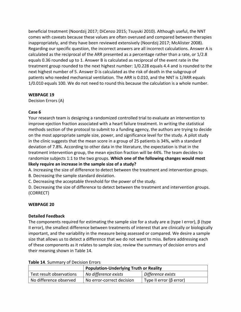
beneficial treatment (Noordzij 2017; DiCenzo 2015; Tsuyuki 2010). Although useful, the NNT comes with caveats because these values are often overused and compared between therapies inappropriately, and they have been reviewed extensively (Noordzij 2017; McAlister 2008). Regarding our specific question, the incorrect answers are all incorrect calculations. Answer A is calculated as the reciprocal of the ARR presented as a percentage rather than a rate, or 1/2.8 equals 0.36 rounded up to 1. Answer B is calculated as reciprocal of the event rate in the treatment group rounded to the next highest number: 1/0.228 equals 4.4 and is rounded to the next highest number of 5. Answer D is calculated as the risk of death in the subgroup of patients who needed mechanical ventilation. The ARR is 0.010, and the NNT is 1/ARR equals 1/0.010 equals 100. We do not need to round this because the calculation is a whole number. WEBPAGE 19 Decision Errors (A) Case 6 Your research team is designing a randomized controlled trial to evaluate an intervention to improve ejection fraction associated with a heart failure treatment. In writing the statistical methods section of the protocol to submit to a funding agency, the authors are trying to decide on the most appropriate sample size, power, and significance level for the study. A pilot study in the clinic suggests that the mean score in a group of 25 patients is 34%, with a standard deviation of 7.8%. According to other data in the literature, the expectation is that in the treatment intervention group, the mean ejection fraction will be 44%. The team decides to randomize subjects 1:1 to the two groups. Which one of the following changes would most likely require an increase in the sample size of a study? A. Increasing the size of difference to detect between the treatment and intervention groups. B. Decreasing the sample standard deviation. C. Decreasing the acceptable threshold for the power of the study. D. Decreasing the size of difference to detect between the treatment and intervention groups. (CORRECT) WEBPAGE 20 Detailed Feedback The components required for estimating the sample size for a study are α (type I error), β (type II error), the smallest difference between treatments of interest that are clinically or biologically important, and the variability in the measure being assessed or compared. We desire a sample size that allows us to detect a difference that we do not want to miss. Before addressing each of these components as it relates to sample size, review the summary of decision errors and their meaning shown in Table 14. Table 14. Summary of Decision Errors

Population-Underlying Truth or Reality

Test result observations No difference exists Difference exists

No difference observed No error-correct decision Type II error (β error)

Difference observed Type I error (α error) No error-correct decision

By convention, it has become commonplace to set the α of a study at 0.05; therefore, if the p value determined in the study is less than 0.05, statistical significance is concluded. However, just because statistical significance is concluded by the study authors (if the p value is less than 0.05), we do not definitively know that there is an actual difference between the groups being compared. Assuming the study was properly designed and analyzed, there is less than a 5% chance to observe the difference in the sample means if they came from the same population (i.e., 5% of the time, a researcher could conclude that there is a statistically significant difference when one does not actually exist). This statistical error is called a type I or α error, and α is the probability of a type I error. A lower p value does not mean the result is more important or more meaningful but only that it is statistically significant and less likely to be attributable to chance. There have been recent calls to suggest that the conventional threshold of 5% is inappropriately high (O’Connor 2019; Wasserstein 2016). The second type of statistical error a researcher could make is to conclude that there is no statistically significant difference when one does in fact exist (i.e., not rejecting the H0 when it should be rejected). This is called a type II or β error, and β is the probability of a type II error. The power of a study is the ability to detect a difference between study groups if one actually exists, or the probability of making a correct decision when the H0 is false. Study power is indirectly related to the likelihood of making a β error and equals 1 minus β. Therefore, as study power increases, the likelihood of concluding that there is not a difference when there is, in fact, a difference, will decrease. The power of a study depends on the (1) sample size, (2) actual difference between the outcomes of interest (e.g., difference between the actual population means µ1 and µ2), (3) variability around each outcome, and (4) predetermined significance level, α. Because the differences between the population means and the population variance cannot be influenced by the investigator, the only way to increase study power (decrease type II error) without increasing the type I error rate is to increase the sample size. By convention, the type II error rate is generally 0.10 or 0.20, depending on the study, and corresponds with 0.90 and 0.80 study power, respectively. Given the acceptable type II error rate, a difference in the outcomes of interest that would be considered clinically significant, the expected variability in the measure, and the type I error rate, an appropriate sample size can be calculated. Sample size calculation is an important step in properly conducting clinical research (DiCenzo 2015; Tsuyuki 2010). The next parameter of interest for estimating sample size is the smallest effect of interest, or the smallest difference between the two treatments that is clinically and biologically important. Selection of this difference requires a keen clinical perspective about what may be statistically important as well as clinically important. Finally, crucial in estimating sample size is the population variance of the outcome variable. When the outcome variable being collected is continuous and because the population variance is not known, it can be estimated from the sample standard deviation. The standard deviation

can be obtained from the literature or a pilot study. In an earlier question, the mean ejection fraction was obtained from a pilot study in which the mean and standard deviation were 34 plus or minus 11. The minimal difference that was determined to be clinically significant was 10. The question asked in this case deals not with actual calculation of sample size, but with what factors will increase the sample size. As discussed earlier, two essential pieces of the sample size determination that are typically set by convention are α equals 0.05 and β equals 0.2 (so power equals 0.8). The other two pieces of information are variability and the minimal difference that is clinically significant. We can combine the last two parameters into one value called the effect size. When the analysis being performed is like the situation in our interactive case (i.e., we are estimating the sample size in an experiment comparing two means), the effect size (Sormani 2017; Das 2016; Gupta 2016; Noordzij 2010) can be calculated as follows:

𝐸𝑓𝑓𝑒𝑐𝑡 𝑠𝑖𝑧𝑒 = 𝑀𝑒𝑎𝑛 𝑒𝑥𝑝𝑒𝑟𝑖𝑚𝑒𝑛𝑡𝑎𝑙 𝑔𝑟𝑜𝑢𝑝 − 𝑀𝑒𝑎𝑛 𝑐𝑜𝑛𝑡𝑟𝑜𝑙 𝑔𝑟𝑜𝑢𝑝

𝑆𝑡𝑎𝑛𝑑𝑎𝑟𝑑 𝑑𝑒𝑣𝑖𝑎𝑡𝑖𝑜𝑛

As effect size increases, the ability to detect a difference between two means increases (i.e., as the difference between the means goes up or the standard deviation goes down, so does the effect size). The larger the effect size, the fewer subjects that are needed. Figure 1 shows this, describing the relationship between effect size and sample size at a constant α and β (Tsuyuki 2010). Figure 1. Relationship between effect size and sample size at a constant α (0.05) and β (0.2). To extend this discussion, Figure 2 shows the relationship between sample size and power. As evidenced by the figure, with α and effect size constant, as power increases, so does the required sample size.

0

50

100

150

200

250

300

350

400

450

500

0 1 2 3 4 5 6 7 8 9 10

Sam

ple

Siz

e (n

)

Effect Size

Figure 2. Relationship between sample size and power at a constant α (0.05) and effect size (1). To answer the question earlier, Answer C can be addressed by looking at Figure 2. As just discussed in the text, choosing a lower β decreases the study power and reduces the number of subjects required (Answer C is incorrect) (i.e., the investigators are willing to accept a higher risk of a type II error). Answer B similarly would also necessitate a lower sample size. As shown in the effect size equation earlier, decreasing the sample standard deviation would increase the effect size. Figure 1 indicates that this would reduce the sample size required (Answer B is incorrect). The correct answer is thus either A or D. Increasing the size of the difference to detect (i.e., in our situation), increasing the difference in the two means would also increase the effect size and necessitate a smaller sample size (Answer A is incorrect). Finally, decreasing the difference to detect would decrease the difference in the two means, which would increase the effect size and lead to a larger sample size (Answer D is correct). Although this question used effect size to discuss sample size calculations using a two-sided two-sample t-test, there are many other effect size examples and their application to other types of data, as reviewed elsewhere. These include the calculation of effect sizes and sample sizes for binary outcomes such as proportions (Das 2016; Noordzij 2010; Florey 1993). WEBPAGE 21 Sample Size Calculations (A) Case 6 (cont’d) Now that the team understands the components of estimating sample size, they need to apply this to the trial. Recall that they are designing a randomized controlled trial to evaluate an intervention to improve ejection fraction associated with a heart failure treatment. A pilot study in the clinic suggests that the mean score in a group of 25 patients is 34%, with a standard deviation of 7.8%. According to other data in the literature, the expectation is that in the treatment intervention group, the mean ejection fraction will be 44%. The group decides to randomize subjects 1:1 to the two groups. The group’s H0 is that the means of the two

0

10

20

30

40

50

60

70

80

90

100

0 10 20 30 40 50 60 70 80

Po

wer

(%

)

Sample Size (n)

interventions are equal. Which one of the following best describes how many subjects will be required in each group assuming a power of 80% and a two-sided α of 0.05? A. 10 (CORRECT) B. 13 C. 20 D. 22 WEBPAGE 22 Detailed Feedback One of the most common questions for statisticians is how many subjects they need to conduct a study (Sormani 2017). Why do sample size calculations even need to be conducted? Minimizing the number of subjects enrolled in an interventional clinical trial is important to minimize any potential risks associated with the intervention as well as to minimize any costs associated with subject recruitment and retention in a clinical study (Sormani 2017; Das 2016; Gupta 2016; Noordzij 2010). Of course, studying too few subjects may lead to the inability to detect a statistical difference between two treatments and a waste of all of the time and money that went into conducting the trial. Choosing a sample size is as fundamental an aspect of designing a study as is determining factors such as which statistical test to use and the most appropriate primary outcome measure. In essence, these determinations are made in concert at the design phase of a study. As a reminder from the previous discussion, the components required for estimating a study’s sample size are α (type I error), β (type II error), the smallest difference between treatments of interest that is clinically or biologically important, and the variability in the outcome measure being assessed. Choosing a sample size that allows for the detection of a difference is desirable. Two of the most common situations in which a sample size is estimated are the estimation of sample size when a continuous parameter or a binary (yes/no) parameter is being compared. For a continuous variable, as in our current question (ejection fraction), the relevant difference between the two treatments is numeric. The investigator must decide what difference in ejection fractions is clinically significant. For a binary parameter, we can turn to our example earlier in the feature, where we were interested in the impact that adding dexamethasone had on mortality at 28 days. In that case, the binary parameter is yes (alive) and no (death). The estimate of a difference that is clinically important would be what percent difference between the mortality rates is clinically important. Finally, crucial to estimating sample size is the population variance of the outcome variable. When the outcome variable being collected is continuous, and because the population variance is not known, it can be estimated from the sample variance and used in the sample size calculation. The variance can be obtained from the literature or a pilot study. In our question, the mean ejection fraction was obtained from a pilot study in which the mean and standard deviation were 34 plus or minus 7.8%. The minimal difference determined to be clinically significant was 10%.

In the case discussed in this question, we are asked to estimate the sample size for a study comparing two means, which can be calculated with the following formula.

𝑛 = 2 [𝑧1−β + 𝑧1−α/2 ]

2𝜎2

(𝜇1 − 𝜇2)2

where n equals sample size in each group, α is 0.05, β is 0.8, z1-α/2 is 1.96, z1-ß is 0.842, 2 is population variance, and 1 and 2 are the population means of the two groups: control and treatment. The assumptions for using this type of test were reviewed in a previous feature. In addition, the assumption earlier is that a two-sided test is used to estimate the sample size required. If we wished to use a directional hypothesis (which is not being done in this case), a one-sided estimate of sample size could be used. Consult any standard statistics text for additional discussion (e.g., Daniel 2018). A one-sided test would require fewer subjects. We can insert our values in the formula to estimate the sample size. Remember that we do not know the population variance or population means and are using our pilot study and minimal clinically important difference as estimates.

𝑛 = 2 [1.96+0.842]27.82

(34−44)2 = 9.55 or 10 subjects in each group

Given the earlier calculation, 10 subjects are required in each group (Answer A is correct). Although the calculation in Answer B uses a β of 0.10, which is not incorrect, this is not what was asked in this question. Of note, this provides an example to show that lower β values (higher power) would require a larger sample size, from 10 to 13 subjects in each group. Answer C is an inappropriate doubling of the calculated sample size, and Answer D uses an incorrect denominator in the earlier equation. According to the CONSORT statement (Schultz 2010), all clinical trials should ideally report a sample size estimate as part of a written manuscript. The primary end point or outcome variable should be stated clearly. In addition to the primary end point, the necessary assumptions and components of the estimation should be presented. Finally, many studies report post hoc power calculations using the results of the trial. The CONSORT statement and others have criticized this practice and instead call for presentation of confidence intervals about the study outcomes.

statistics in practice: study design and application of

Documents