statistics for biology and health -...
TRANSCRIPT

Statistics for Biology and HealthSeries EditorsM. Gail, K. Krickeberg, J. Samet, A. Tsiatis, W. Wong

David G. KleinbaumMitchel Klein
Survival AnalysisA Self-Learning Text
Second Edition

David G. KleinbaumDepartment of EpidemiologyRollins School of Public Health at
Emory University1518 Clifton Road NEAtlanta GA 30306Email: [email protected]
Mitchel KleinDepartment of EpidemiologyRollins School of Public Health at
Emory University1518 Clifton Road NEAtlanta GA 30306Email: [email protected]
Series EditorsM. GailNational Cancer InstituteRockville, MD 20892USA
K. KrickebergLe ChateletF-63270 ManglieuFrance
J. SametDepartment of EpidemiologySchool of Public HealthJohns Hopkins University615 Wolfe StreetBaltimore, MD 21205USA
A. TsiatisDepartment of StatisticsNorth Carolina State UniversityRaleigh, NC 27695USA
Wing WongDepartment of StatisticsStanford UniversityStanford, CA 94305USA
SAS® and all other SAS Institute Inc. product or service names are registered trademarks or trademarksof SAS Institute Inc. in the USA and other countries. ® indicates USA registration.
SPSS® is a registered trademark of SPSS Inc.
STATA® and the STATA® logo are registered trademarks of StataCorp LP.
Library of Congress Control Number: 2005925181
ISBN-10: 0-387-23918-9 Printed on acid-free paper.ISBN-13: 978-0387-23918-7
© 2005, 1996 Springer Science+Business Media, Inc.All rights reserved. This work may not be translated or copied in whole or in part without the writtenpermission of the publisher (Springer Science+Business Media, Inc., 233 Spring Street, New York, NY10013, USA), except for brief excerpts in connection with reviews or scholarly analysis. Use in connec-tion with any form of information storage and retrieval, electronic adaptation, computer software, or bysimilar or dissimilar methodology now known or hereafter developed is forbidden.The use in this publication of trade names, trademarks, service marks, and similar terms, even if theyare not identified as such, is not to be taken as an expression of opinion as to whether or not they aresubject to proprietary rights.
Printed in the United States of America. (TechBooks/HAM)
9 8 7 6 5 4 3 2 1
springeronline.com

Survival AnalysisA Self-Learning Text
SpringerNew YorkBerlinHeidelbergHong KongLondonMilanParisTokyo

David G. Kleinbaum Mitchel Klein
Survival Analysis
A Self-Learning Text
Second Edition

To Rosa Parks
Nelson Mandela
Dean Smith
Sandy Koufax
And
countless other persons, well-known or unknown,who have had the courage to stand up for their beliefs for thebenefit of humanity.

PrefaceThis is the second edition of this text on survival analysis,originally published in 1996. As in the first edition, each chap-ter contains a presentation of its topic in “lecture-book” for-mat together with objectives, an outline, key formulae, prac-tice exercises, and a test. The “lecture-book” format has asequence of illustrations and formulae in the left column ofeach page and a script in the right column. This format allowsyou to read the script in conjunction with the illustrations andformulae that high-light the main points, formulae, or exam-ples being presented.
This second edition has expanded the first edition by addingthree new chapters and a revised computer appendix. Thethree new chapters are:
Chapter 7. Parametric Survival ModelsChapter 8. Recurrent Event Survival AnalysisChapter 9. Competing Risks Survival Analysis
Chapter 7 extends survival analysis methods to a class of sur-vival models, called parametric models, in which the distri-bution of the outcome (i.e., the time to event) is specified interms of unknown parameters. Many such parametric modelsare acceleration failure time models, which provide an alter-native measure to the hazard ratio called the “accelerationfactor”. The general form of the likelihood for a parametricmodel that allows for left, right, or interval censored data isalso described. The chapter concludes with an introductionto frailty models.
Chapter 8 considers survival events that may occur more thanonce over the follow-up time for a given subject. Such eventsare called “recurrent events”. Analysis of such data can becarried out using a Cox PH model with the data layout aug-mented so that each subject has a line of data for each re-current event. A variation of this approach uses a stratifiedCox PH model, which stratifies on the order in which recur-rent events occur. The use of “robust variance estimates” arerecommended to adjust the variances of estimated model co-efficients for correlation among recurrent events on the samesubject.

viii Preface
Chapter 9 considers survival data in which each subject canexperience only one of several different types of events (“com-peting risks”) over follow-up. Modeling such data can be car-ried out using a Cox model, a parametric survival model or amodel which uses cumulative incidence (rather than survival).
The Computer Appendix in the first edition of this text hasnow been revised and extended to provide step-by-step in-structions for using the computer packages STATA (version7.0), SAS (version 8.2), and SPSS (version 11.5) to carry outthe survival analyses presented in the main text. These com-puter packages are described in separate self-contained sec-tions of the Computer Appendix, with the analysis of the samedatasets illustrated in each section. The SPIDA package usedin the first edition is no longer active and has therefore beenomitted from the appendix and computer output in the maintext.
In addition to the above new material, the original six chap-ters have been modified slightly to correct for errata in the firstedition, to clarify certain issues, and to add theoretical back-ground, particularly regarding the formulation of the (partial)likelihood functions for the Cox PH (Chapter 3) and extendedCox (Chapter 6) models.
The authors’ website for this textbook has the following web-link: http://www.sph.emory.edu/∼dkleinb/surv2.htm
This website includes information on how to order thissecond edition from the publisher and a freely downloadablezip-file containing data-files for examples used in the text-book.
Suggestionsfor Use
This text was originally intended for self-study, but in the nineyears since the first edition was published, it has also been ef-fectively used as a text in a standard lecture-type classroomformat. The text may also be use to supplement material cov-ered in a course or to review previously learned material ina self-instructional course or self-planned learning activity.A more individualized learning program may be particularlysuitable to a working professional who does not have the timeto participate in a regularly scheduled course.

Preface ix
In working with any chapter, the learner is encouraged first toread the abbreviated outline and the objectives and then workthrough the presentation. The reader is then encouraged toread the detailed outline for a summary of the presentation,work through the practice exercises, and, finally, complete thetest to check what has been learned.
RecommendedPreparation
The ideal preparation for this text on survival analysis is acourse on quantitative methods in epidemiology and a coursein applied multiple regression. Also, knowledge of logistic re-gression, modeling strategies, and maximum likelihood tech-niques is crucial for the material on the Cox and parametricmodels described in chapters 3–9.
Recommended references on these subjects, with suggestedchapter readings are:
Kleinbaum D, Kupper L, Muller K, and Nizam A, AppliedRegression Analysis and Other Multivariable Methods,Third Edition, Duxbury Press, Pacific Grove, 1998, Chapters1–16, 22–23
Kleinbaum D, Kupper L and Morgenstern H, EpidemiologicResearch: Principles and Quantitative Methods, JohnWiley and Sons, Publishers, New York, 1982, Chapters 20–24.
Kleinbaum D and Klein M, Logistic Regression: A Self-Learning Text, Second Edition, Springer-Verlag Publishers,New York, Chapters 4–7, 11.
Kleinbaum D, ActivEpi-A CD Rom Electronic Textbook onFundamentals of Epidemiology, Springer-Verlag Publish-ers, New York, 2002, Chapters 13–15.
A first course on the principles of epidemiologic researchwould be helpful, since all chapters in this text are writtenfrom the perspective of epidemiologic research. In particular,the reader should be familiar with the basic characteristics ofepidemiologic study designs, and should have some idea ofthe frequently encountered problem of controlling for con-founding and assessing interaction/effect modification. Theabove reference, ActivEpi, provides a convenient and hope-fully enjoyable way to review epidemiology.

AcknowledgmentsWe wish to thank Allison Curry for carefully reviewing andediting the previous edition’s first six chapters for clarity ofcontent and errata. We also thank several faculty and MPHand PhD students in the Department of Epidemiology whohave provided feedback on the first edition of this text aswell as new chapters in various stages of development. Thisincludes Michael Goodman, Mathew Strickland, and SarahTinker. We thank Dr. Val Gebski of the NHMRC ClinicalTrials Centre, Sydney, Australia, for providing continued in-sight on current methods of survival analysis and review ofnew additions to the manuscript for this edition.
Finally, David Kleinbaum and Mitch Klein thank EdnaKleinbaum and Becky Klein for their love, support, compan-ionship, and sense of humor during the writing of this secondedition.
ContentsPreface vii
Acknowledgments xi
Chapter 1 Introduction to Survival Analysis 1
Introduction 2Abbreviated Outline 2Objectives 3Presentation 4Detailed Outline 34Practice Exercises 38Test 40Answers to Practice Exercises 42
Chapter 2 Kaplan–Meier Survival Curves and theLog–Rank Test 45
Introduction 46Abbreviated Outline 46Objectives 47Presentation 48Detailed Outline 70Practice Exercises 73Test 77Answers to Practice Exercises 79Appendix: Matrix Formula for the Log–Rank Statisticfor Several Groups 82
Chapter 3 The Cox Proportional Hazards Model and ItsCharacteristics 83
Introduction 84Abbreviated Outline 84Objectives 85Presentation 86Detailed Outline 117Practice Exercises 119Test 123Answers to Practice Exercises 127

xiv Contents
Chapter 4 Evaluating the Proportional HazardsAssumption 131
Introduction 132Abbreviated Outline 132Objectives 133Presentation 134Detailed Outline 158Practice Exercises 161Test 164Answers to Practice Exercises 167
Chapter 5 The Stratified Cox Procedure 173
Introduction 174Abbreviated Outline 174Objectives 175Presentation 176Detailed Outline 198Practice Exercises 201Test 204Answers to Practice Exercises 207
Chapter 6 Extension of the Cox Proportional HazardsModel for Time-Dependent Variables 211
Introduction 212Abbreviated Outline 212Objectives 213Presentation 214Detailed Outline 246Practice Exercises 249Test 253Answers to Practice Exercises 255
Chapter 7 Parametric Survival Models 257
Introduction 258Abbreviated Outline 258Objectives 259Presentation 260Detailed Outline 313Practice Exercises 319Test 324Answers to Practice Exercises 327
Contents xv
Chapter 8 Recurrent Event Survival Analysis 331
Introduction 332Abbreviated Outline 332Objectives 333Presentation 334Detailed Outline 371Practice Exercises 377Test 381Answers to Practice Exercises 389
Chapter 9 Competing Risks Survival Analysis 391
Introduction 392Abbreviated Outline 394Objectives 395Presentation 396Detailed Outline 440Practice Exercises 447Test 452Answers to Practice Exercises 458
Computer Appendix: Survival Analysis onthe Computer 463
A. STATA 465B. SAS 508C. SPSS 542
Test Answers 557
References 581
Index 585

1 Introductionto SurvivalAnalysis
1

2 1. Introduction to Survival Analysis
Introduction This introduction to survival analysis gives a descriptiveoverview of the data analytic approach called survival analy-sis. This approach includes the type of problem addressed bysurvival analysis, the outcome variable considered, the needto take into account “censored data,” what a survival func-tion and a hazard function represent, basic data layouts fora survival analysis, the goals of survival analysis, and someexamples of survival analysis.
Because this chapter is primarily descriptive in content, noprerequisite mathematical, statistical, or epidemiologic con-cepts are absolutely necessary. A first course on the principlesof epidemiologic research would be helpful. It would also behelpful if the reader has had some experience reading math-ematical notation and formulae.
AbbreviatedOutline
The outline below gives the user a preview of the material tobe covered by the presentation. A detailed outline for reviewpurposes follows the presentation.
I. What is survival analysis? (pages 4–5)II. Censored data (pages 5–8)
III. Terminology and notation (pages 8–14)IV. Goals of survival analysis (page 15)V. Basic data layout for computer (pages 15–19)
VI. Basic data layout for understanding analysis(pages 19–24)
VII. Descriptive measures of survival experience(pages 24–26)
VIII. Example: Extended remission data (pages 26–29)IX. Multivariable example (pages 29–31)X. Math models in survival analysis (pages 31–33)
Objectives 3
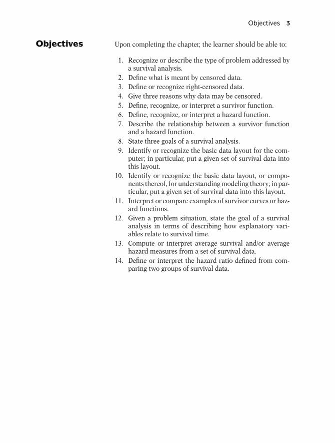
Objectives Upon completing the chapter, the learner should be able to:
1. Recognize or describe the type of problem addressed bya survival analysis.
2. Define what is meant by censored data.3. Define or recognize right-censored data.4. Give three reasons why data may be censored.5. Define, recognize, or interpret a survivor function.6. Define, recognize, or interpret a hazard function.7. Describe the relationship between a survivor function
and a hazard function.8. State three goals of a survival analysis.9. Identify or recognize the basic data layout for the com-
puter; in particular, put a given set of survival data intothis layout.
10. Identify or recognize the basic data layout, or compo-nents thereof, for understanding modeling theory; in par-ticular, put a given set of survival data into this layout.
11. Interpret or compare examples of survivor curves or haz-ard functions.
12. Given a problem situation, state the goal of a survivalanalysis in terms of describing how explanatory vari-ables relate to survival time.
13. Compute or interpret average survival and/or averagehazard measures from a set of survival data.
14. Define or interpret the hazard ratio defined from com-paring two groups of survival data.
4 1. Introduction to Survival Analysis
Presentation
FOCUS
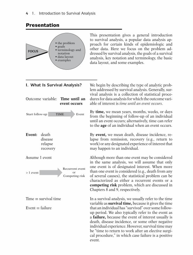
• the problem• goals• terminology and notation• data layout• examples
This presentation gives a general introductionto survival analysis, a popular data analysis ap-proach for certain kinds of epidemiologic andother data. Here we focus on the problem ad-dressed by survival analysis, the goals of a survivalanalysis, key notation and terminology, the basicdata layout, and some examples.
I. What Is Survival Analysis?
Outcome variable: Time until anevent occurs
We begin by describing the type of analytic prob-lem addressed by survival analysis. Generally, sur-vival analysis is a collection of statistical proce-dures for data analysis for which the outcome vari-able of interest is time until an event occurs.
TIMEStart follow-up EventBy time, we mean years, months, weeks, or daysfrom the beginning of follow-up of an individualuntil an event occurs; alternatively, time can referto the age of an individual when an event occurs.
Event: deathdiseaserelapserecovery
By event, we mean death, disease incidence, re-lapse from remission, recovery (e.g., return towork) or any designated experience of interest thatmay happen to an individual.
Assume 1 event
> 1 eventRecurrent event
orCompeting risk
Although more than one event may be consideredin the same analysis, we will assume that onlyone event is of designated interest. When morethan one event is considered (e.g., death from anyof several causes), the statistical problem can becharacterized as either a recurrent events or acompeting risk problem, which are discussed inChapters 8 and 9, respectively.
Time ≡ survival time
Event ≡ failure
In a survival analysis, we usually refer to the timevariable as survival time, because it gives the timethat an individual has “survived” over some follow-up period. We also typically refer to the event asa failure, because the event of interest usually isdeath, disease incidence, or some other negativeindividual experience. However, survival time maybe “time to return to work after an elective surgi-cal procedure,” in which case failure is a positiveevent.

Presentation: II. Censored Data 5
Leukemia patients/time in remis-sion (weeks)
Disease-free cohort/time until heartdisease (years)
Elderly (60+) population/time untildeath (years)Parolees (recidivism study)/timeuntil rearrest (weeks)
Heart transplants/time until death(months)
EXAMPLE
1.
2.
3.
4.
5.
Five examples of survival analysis problems arebriefly mentioned here. The first is a study that fol-lows leukemia patients in remission over severalweeks to see how long they stay in remission. Thesecond example follows a disease-free cohort ofindividuals over several years to see who developsheart disease. A third example considers a 13-yearfollow-up of an elderly population (60+ years) tosee how long subjects remain alive. A fourth ex-ample follows newly released parolees for severalweeks to see whether they get rearrested. This typeof problem is called a recidivism study. The fifthexample traces how long patients survive after re-ceiving a heart transplant.
All of the above examples are survival analysisproblems because the outcome variable is timeuntil an event occurs. In the first example, involv-ing leukemia patients, the event of interest (i.e.,failure) is “going out of remission,” and the out-come is “time in weeks until a person goes outof remission.” In the second example, the eventis “developing heart disease,” and the outcome is“time in years until a person develops heart dis-ease.” In the third example, the event is “death”and the outcome is “time in years until death.”Example four, a sociological rather than a medi-cal study, considers the event of recidivism (i.e.,getting rearrested), and the outcome is “time inweeks until rearrest.” Finally, the fifth exampleconsiders the event “death,” with the outcome be-ing “time until death (in months from receiving atransplant).”
We will return to some of these examples later inthis presentation and in later presentations.
II. Censored Data Most survival analyses must consider a keyanalytical problem called censoring. In essence,censoring occurs when we have some informationabout individual survival time, but we don’t knowthe survival time exactly.
Censoring: don’t know survivaltime exactly

6 1. Introduction to Survival Analysis
Leukemia patients in remission:
X
Studyend
Studystart
EXAMPLE As a simple example of censoring, considerleukemia patients followed until they go out of re-mission, shown here as X. If for a given patient,the study ends while the patient is still in remission(i.e., doesn’t get the event), then that patient’s sur-vival time is considered censored. We know that,for this person, the survival time is at least as longas the period that the person has been followed,but if the person goes out of remission after thestudy ends, we do not know the complete survivaltime.
Why censor?
1. study ends—no event2. lost to follow-up3. withdraws
There are generally three reasons why censoringmay occur:
(1) a person does not experience the event beforethe study ends;
(2) a person is lost to follow-up during the studyperiod;
(3) a person withdraws from the study becauseof death (if death is not the event of interest) orsome other reason (e.g., adverse drug reactionor other competing risk)
EXAMPLE
A
B
C
D
E
F
T = 5
T = 12
T = 3.5
T = 8
T = 6
2 4 6 8 10 12Weeks
T = 3.5X
X
Study end
Withdrawn
Study end
Lost
These situations are graphically illustrated here.The graph describes the experience of several per-sons followed over time. An X denotes a personwho got the event.
Person A, for example, is followed from the startof the study until getting the event at week 5; hissurvival time is 5 weeks and is not censored.
Person B also is observed from the start of thestudy but is followed to the end of the 12-weekstudy period without getting the event; the survivaltime here is censored because we can say only thatit is at least 12 weeks.
X Event occurs Person C enters the study between the second andthird week and is followed until he withdrawsfrom the study at 6 weeks; this person’s survivaltime is censored after 3.5 weeks.
Person D enters at week 4 and is followed for theremainder of the study without getting the event;this person’s censored time is 8 weeks.

Presentation: II. Censored Data 7
Person E enters the study at week 3 and is fol-lowed until week 9, when he is lost to follow-up;his censored time is 6 weeks.
Person F enters at week 8 and is followed untilgetting the event at week 11.5. As with person A,there is no censoring here; the survival time is3.5 weeks.
SUMMARYEvent: A, FCensored: B, C, D, E
In summary, of the six persons observed, two getthe event (persons A and F) and four are censored(B, C, D, and E).
PersonSurvival
timeFailed (1);
censored (0)
A
B
C
D
E
F
5
12
3.5
8
6
3.5
1
0
0
0
0
1
A table of the survival time data for the six personsin the graph is now presented. For each person,we have given the corresponding survival time upto the event’s occurrence or up to censorship. Wehave indicated in the last column whether thistime was censored or not (with 1 denoting failedand 0 denoting censored). For example, the datafor person C is a survival time of 3.5 and a cen-sorship indicator of 0, whereas for person F thesurvival time is 3.5 and the censorship indicator is1. This table is a simplified illustration of the typeof data to be analyzed in a survival analysis.
RIGHTCENSORED
A
B
C
D
E
F
2 4 6 8 10 12Weeks
X
X
Study end
Withdrawn
Study end
Lost
Notice in our example that for each of the fourpersons censored, we know that the person’s exactsurvival time becomes incomplete at the right sideof the follow-up period, occurring when the studyends or when the person is lost to follow-up or iswithdrawn. We generally refer to this kind of dataas right-censored. For these data, the completesurvival time interval, which we don’t really know,has been cut off (i.e., censored) at the right side ofthe observed survival time interval. Although datacan also be left-censored, most survival data isright-censored.
8 1. Introduction to Survival Analysis
True survival time
Observed survival time
Study start HIV + testHIV exposure
X
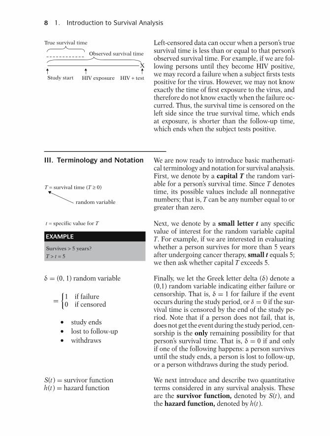
Left-censored data can occur when a person’s truesurvival time is less than or equal to that person’sobserved survival time. For example, if we are fol-lowing persons until they become HIV positive,we may record a failure when a subject firsts testspositive for the virus. However, we may not knowexactly the time of first exposure to the virus, andtherefore do not know exactly when the failure oc-curred. Thus, the survival time is censored on theleft side since the true survival time, which endsat exposure, is shorter than the follow-up time,which ends when the subject tests positive.
III. Terminology and Notation We are now ready to introduce basic mathemati-cal terminology and notation for survival analysis.First, we denote by a capital T the random vari-able for a person’s survival time. Since T denotestime, its possible values include all nonnegativenumbers; that is, T can be any number equal to orgreater than zero.
T = survival time (T ≥ 0)
random variable
Survives > 5 years?
T > t = 5
EXAMPLE
t = specific value for T Next, we denote by a small letter t any specificvalue of interest for the random variable capitalT. For example, if we are interested in evaluatingwhether a person survives for more than 5 yearsafter undergoing cancer therapy, small t equals 5;we then ask whether capital T exceeds 5.
δ = (0, 1) random variable
={
1 if failure0 if censored
� study ends� lost to follow-up� withdraws
Finally, we let the Greek letter delta (δ) denote a(0,1) random variable indicating either failure orcensorship. That is, δ = 1 for failure if the eventoccurs during the study period, or δ = 0 if the sur-vival time is censored by the end of the study pe-riod. Note that if a person does not fail, that is,does not get the event during the study period, cen-sorship is the only remaining possibility for thatperson’s survival time. That is, δ = 0 if and onlyif one of the following happens: a person survivesuntil the study ends, a person is lost to follow-up,or a person withdraws during the study period.
S(t) = survivor functionh(t) = hazard function
We next introduce and describe two quantitativeterms considered in any survival analysis. Theseare the survivor function, denoted by S(t), andthe hazard function, denoted by h(t).
Presentation: III. Terminology and Notation 9
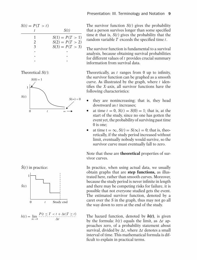
S(t) = P (T > t)t S(t)
1 S(1) = P (T > 1)2 S(2) = P (T > 2)3 S(3) = P (T > 3)· ·· ·· ·
The survivor function S(t) gives the probabilitythat a person survives longer than some specifiedtime t: that is, S(t) gives the probability that therandom variable T exceeds the specified time t.
The survivor function is fundamental to a survivalanalysis, because obtaining survival probabilitiesfor different values of t provides crucial summaryinformation from survival data.
Theoretical S(t):
0 t
S(0) = 1
S(t)
∞
S(∞) = 0
1
Theoretically, as t ranges from 0 up to infinity,the survivor function can be graphed as a smoothcurve. As illustrated by the graph, where t iden-tifies the X -axis, all survivor functions have thefollowing characteristics:
� they are nonincreasing; that is, they headdownward as t increases;� at time t = 0, S(t) = S(0) = 1; that is, at thestart of the study, since no one has gotten theevent yet, the probability of surviving past time0 is one;� at time t = ∞, S(t) = S(∞) = 0; that is, theo-retically, if the study period increased withoutlimit, eventually nobody would survive, so thesurvivor curve must eventually fall to zero.
Note that these are theoretical properties of sur-vivor curves.
S(t) in practice:
1
0 Study endt
S(t)
In practice, when using actual data, we usuallyobtain graphs that are step functions, as illus-trated here, rather than smooth curves. Moreover,because the study period is never infinite in lengthand there may be competing risks for failure, it ispossible that not everyone studied gets the event.The estimated survivor function, denoted by acaret over the S in the graph, thus may not go allthe way down to zero at the end of the study.
h(t) = lim�t→0
P (t ≤ T < t + �t|T ≥ t)�t
The hazard function, denoted by h(t), is givenby the formula: h(t) equals the limit, as �t ap-proaches zero, of a probability statement aboutsurvival, divided by �t, where �t denotes a smallinterval of time. This mathematical formula is dif-ficult to explain in practical terms.

10 1. Introduction to Survival Analysis
h(t) = instantaneous potential
FOCUS S(t) : not failingh(t) : failing
Before getting into the specifics of the formula,we give a conceptual interpretation. The hazardfunction h(t) gives the instantaneous potentialper unit time for the event to occur, given thatthe individual has survived up to time t. Notethat, in contrast to the survivor function, whichfocuses on not failing, the hazard function focuseson failing, that is, on the event occurring. Thus, insome sense, the hazard function can be consideredas giving the opposite side of the information givenby the survivor function.
60 To get an idea of what we mean by instantaneouspotential, consider the concept of velocity. If, forexample, you are driving in your car and you seethat your speedometer is registering 60 mph, whatdoes this reading mean? It means that if in thenext hour, you continue to drive this way, withthe speedometer exactly on 60, you would cover60 miles. This reading gives the potential, at themoment you have looked at your speedometer,for how many miles you will travel in the nexthour. However, because you may slow down orspeed up or even stop during the next hour, the60-mph speedometer reading does not tell youthe number of miles you really will cover in thenext hour. The speedometer tells you only howfast you are going at a given moment; that is, theinstrument gives your instantaneous potential orvelocity.
Instantaneous potential
Velocity at time t
h(t)
Similar to the idea of velocity, a hazard functionh(t) gives the instantaneous potential at time tfor getting an event, like death or some diseaseof interest, given survival up to time t. The givenpart, that is, surviving up to time t, is analo-gous to recognizing in the velocity example thatthe speedometer reading at a point in time in-herently assumes that you have already traveledsome distance (i.e., survived) up to the time of thereading.

Presentation: III. Terminology and Notation 11
h(t) = limP(t ≤ T< t + ∆ t | T ≥ t)
∆ t∆t→0
Given
Conditional probabilities: P (A|B)
P (t ≤ T < t + �t | T ≥ t)= P(individual fails in the interval
[t, t + �t] | survival up to time t)
In mathematical terms, the given part of the for-mula for the hazard function is found in the proba-bility statement—the numerator to the right of thelimit sign. This statement is a conditional prob-ability because it is of the form, “P of A, givenB,” where the P denotes probability and wherethe long vertical line separating A from B denotes“given.” In the hazard formula, the conditionalprobability gives the probability that a person’ssurvival time, T, will lie in the time interval be-tween t and t + �t, given that the survival timeis greater than or equal to t. Because of the givensign here, the hazard function is sometimes calleda conditional failure rate.
Hazard function ≡ conditionalfailure rate
limP(t ≤ T < t + ∆ t | T ≥ t)
∆ t∆ t→0
Probability per unit time
Rate: 0 to ∞
We now explain why the hazard is a rate ratherthan a probability. Note that in the hazard func-tion formula, the expression to the right of thelimit sign gives the ratio of two quantities. Thenumerator is the conditional probability we justdiscussed. The denominator is �t, which denotesa small time interval. By this division, we obtain aprobability per unit time, which is no longer aprobability but a rate. In particular, the scalefor this ratio is not 0 to 1, as for a probability,but rather ranges between 0 and infinity, and de-pends on whether time is measured in days, weeks,months, or years, etc.
P = P (t ≤ T < t + � t|T ≥ t)
P �t P/�t = rate
13
12
day1/31/2
= 0.67/day
13
114
week1/31/14
= 4.67/week
For example, if the probability, denoted here byP , is 1/3, and the time interval is one-half a day,then the probability divided by the time intervalis 1/3 divided by 1/2, which equals 0.67 per day.As another example, suppose, for the same prob-ability of 1/3, that the time interval is consideredin weeks, so that 1/2 day equals 1/14 of a week.Then the probability divided by the time intervalbecomes 1/3 over 1/14, which equals 14/3, or 4.67per week. The point is simply that the expression Pdivided by �t at the right of the limit sign does notgive a probability. The value obtained will givea different number depending on the units oftime used, and may even give a number largerthan one.

12 1. Introduction to Survival Analysis
h(t) = lim P (t ≤ T< t + ∆t | T ≥ t)∆t∆t→0
Givesinstantaneouspotential
When we take the limit of the right-side expres-sion as the time interval approaches zero, we areessentially getting an expression for the instanta-neous probability of failing at time t per unit time.Another way of saying this is that the conditionalfailure rate or hazard function h(t) gives the in-stantaneous potential for failing at time t per unittime, given survival up to time t.
0 t
h(t)
Hazard functions
� h(t) ≥ 0� h(t) has no upper bound
As with a survivor function, the hazard functionh(t) can be graphed as t ranges over various values.The graph at the left illustrates three different haz-ards. In contrast to a survivor function, the graphof h(t) does not have to start at 1 and go down tozero, but rather can start anywhere and go up anddown in any direction over time. In particular, fora specified value of t, the hazard function h(t) hasthe following characteristics:
� it is always nonnegative, that is, equal to orgreater than zero;� it has no upper bound.
These two features follow from the ratio expres-sion in the formula for h(t), because both the prob-ability in the numerator and the �t in the denom-inator are nonnegative, and since �t can rangebetween 0 and ∞.
Constant hazard(exponential model)
h(t) for healthypersons
EXAMPLE
t
λ
1
Now we show some graphs of different types ofhazard functions. The first graph given shows aconstant hazard for a study of healthy persons.In this graph, no matter what value of t is spec-ified, h(t) equals the same value—in this exam-ple, λ. Note that for a person who continues to behealthy throughout the study period, his/her in-stantaneous potential for becoming ill at any timeduring the period remains constant throughoutthe follow-up period. When the hazard functionis constant, we say that the survival model is ex-ponential. This term follows from the relation-ship between the survivor function and the hazardfunction. We will return to this relationship later.
Presentation: III. Terminology and Notation 13
t
h(t) for leukemiapatients
↑ Weibull
t
h(t) for personsrecovering fromsurgery
↓ Weibull
t
h(t) for TBpatients
↑ ↓ lognormal
EXAMPLE (continued)
2
3
4
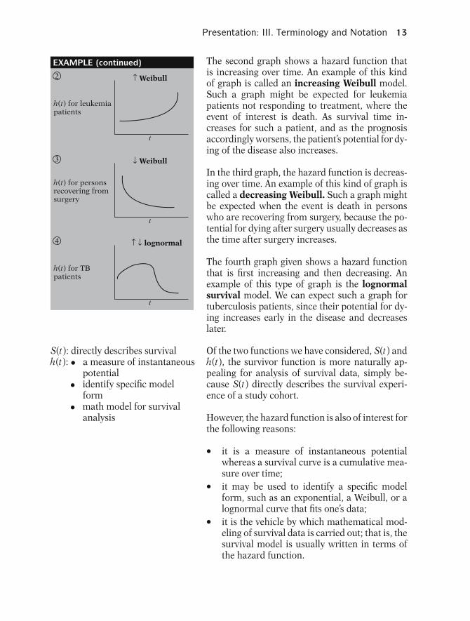
The second graph shows a hazard function thatis increasing over time. An example of this kindof graph is called an increasing Weibull model.Such a graph might be expected for leukemiapatients not responding to treatment, where theevent of interest is death. As survival time in-creases for such a patient, and as the prognosisaccordingly worsens, the patient’s potential for dy-ing of the disease also increases.
In the third graph, the hazard function is decreas-ing over time. An example of this kind of graph iscalled a decreasing Weibull. Such a graph mightbe expected when the event is death in personswho are recovering from surgery, because the po-tential for dying after surgery usually decreases asthe time after surgery increases.
The fourth graph given shows a hazard functionthat is first increasing and then decreasing. Anexample of this type of graph is the lognormalsurvival model. We can expect such a graph fortuberculosis patients, since their potential for dy-ing increases early in the disease and decreaseslater.
S(t): directly describes survivalh(t): • a measure of instantaneous
potential• identify specific model
form• math model for survival
analysis
Of the two functions we have considered, S(t) andh(t), the survivor function is more naturally ap-pealing for analysis of survival data, simply be-cause S(t) directly describes the survival experi-ence of a study cohort.
However, the hazard function is also of interest forthe following reasons:
� it is a measure of instantaneous potentialwhereas a survival curve is a cumulative mea-sure over time;� it may be used to identify a specific modelform, such as an exponential, a Weibull, or alognormal curve that fits one’s data;� it is the vehicle by which mathematical mod-eling of survival data is carried out; that is, thesurvival model is usually written in terms ofthe hazard function.

14 1. Introduction to Survival Analysis
Relationship of S(t) and h(t):If you know one, you can determinethe other.
h(t) = λ if and only if S(t) = e−λt
EXAMPLE
Regardless of which function S(t) or h(t) oneprefers, there is a clearly defined relationshipbetween the two. In fact, if one knows the formof S(t), one can derive the corresponding h(t), andvice versa. For example, if the hazard function isconstant—i.e., h(t) = λ, for some specific valueλ—then it can be shown that the correspondingsurvival function is given by the following for-mula: S(t) equals e to the power minus λ times t.
General formulae:
S(t) = exp[−
∫ t
0h(u)du
]
h(t) = −[
d S(t)/dtS(t)
]
More generally, the relationship between S(t) andh(t) can be expressed equivalently in either of twocalculus formulae shown here.
The first of these formulae describes how the sur-vivor function S(t) can be written in terms of an in-tegral involving the hazard function. The formulasays that S(t) equals the exponential of the nega-tive integral of the hazard function between inte-gration limits of 0 and t.
The second formula describes how the haz-ard function h(t) can be written in terms of aderivative involving the survivor function. Thisformula says that h(t) equals minus the derivativeof S(t) with respect to t divided by S(t).
h(t)S(t)In any actual data analysis a computer programcan make the numerical transformation from S(t)to h(t), or vice versa, without the user ever havingto use either formula. The point here is simply thatif you know either S(t) or h(t), you can get theother directly.
SUMMARY
T = survival time randomvariable
t = specific value of Tδ = (0, 1) variable for failure/
censorshipS(t) = survivor functionh(t) = hazard function
At this point, we have completed our discussionof key terminology and notation. The key no-tation is T for the survival time variable, tfor a specified value of T, and δ for the di-chotomous variable indicating event occur-rence or censorship. The key terms are thesurvivor function S(t) and the hazard func-tion h(t), which are in essence opposed con-cepts, in that the survivor function focuses onsurviving whereas the hazard function focuseson failing, given survival up to a certain timepoint.

Presentation: V. Basic Data Layout for Computer 15
IV. Goals of Survival Analysis We now state the basic goals of survival analysis.
Goal 1: To estimate and interpret survivor and/orhazard functions from survival data.
Goal 2: To compare survivor and/or hazard func-tions.
Goal 3: To assess the relationship of explanatoryvariables to survival time.
S(t) S(t)
t t
Regarding the first goal, consider, for example, thetwo survivor functions pictured at the left, whichgive very different interpretations. The functionfarther on the left shows a quick drop in survivalprobabilities early in follow-up but a leveling offthereafter. The function on the right, in contrast,shows a very slow decrease in survival probabili-ties early in follow-up but a sharp decrease lateron.
S(t)
Placebo
Treatment
t6
We compare survivor functions for a treatmentgroup and a placebo group by graphing these func-tions on the same axis. Note that up to 6 weeks,the survivor function for the treatment group liesabove that for the placebo group, but thereafterthe two functions are at about the same level.This dual graph indicates that up to 6 weeks thetreatment is more effective for survival than theplacebo but has about the same effect thereafter.
Goal 3: Use math modeling, e.g., Coxproportional hazards
Goal 3 usually requires using some form of math-ematical modeling, for example, the Cox propor-tional hazards approach, which will be the subjectof subsequent modules.
V. Basic Data Layoutfor Computer
We previously considered some examples of sur-vival analysis problems and a simple data set in-volving six persons. We now consider the generaldata layout for a survival analysis. We will providetwo types of data layouts, one giving the form ap-propriate for computer use, and the other givingthe form that helps us understand how a survivalanalysis works.
Two types of data layouts:
� for computer use� for understanding

16 1. Introduction to Survival Analysis
For computer:
Indiv. #
12•
•
•
5•
•
•
8•
•
•
n
t
t1t2
t5 = 3 got event
t8 = 3 censored
X1
X12
X22
X11
X21
Xn1 Xn2 Xnp
X2 Xp• • •
• • •
X1p• • •
X2p• • •
•
•
•
•
•
•
•
•
•
δ
δ1
δ2
δntn
We start by providing, in the table shown here, thebasic data layout for the computer. Assume that wehave a data set consisting of n persons. The firstcolumn of the table identifies each person from 1,starting at the top, to n, at the bottom.
The remaining columns after the first one providesurvival time and other information for each per-son. The second column gives the survival timeinformation, which is denoted t1 for individual 1,t2 for individual 2, and so on, up to tn for individualn. Each of these t ’s gives the observed survival timeregardless of whether the person got the event oris censored. For example, if person 5 got the eventat 3 weeks of follow-up, then t5 = 3; on the otherhand, if person 8 was censored at 3 weeks, withoutgetting the event, then t8 = 3 also.
To distinguish persons who get the event fromthose who are censored, we turn to the third col-umn, which gives the information for status (i.e.δ) the dichotomous variable that indicates censor-ship status.
Indiv. #
12•
•
•
5•
•
•
8•
•
•
n
t
t1t2
t5 = 3 δ5 = 1
t8 = 3 δ8 = 0
X1
X12
X22
X11
X21
Xn1 Xn2 Xnp
X2 Xp• • •
• • •
X1p• • •
X2p• • •
•
•
•
•
•
•
•
•
•
δ
δ1
δ2
δntn
Xi = Age, E, or Age × Race
Failurestatus
Explanatoryvariables
n
1∑ δj= # failures
Thus, δ1 is 1 if person 1 gets the event or is 0 ifperson 1 is censored; δ2 is 1 or 0 similarly, and soon, up through δn. In the example just considered,person 5, who failed at 3 weeks, has a δ of 1; thatis, δ5 equals 1. In contrast, person 8, who was cen-sored at 3 weeks, has a δ of 0; that is, δ8 equals 0.
Note that if all of the δ j in this column are addedup, their sum will be the total number of failures inthe data set. This total will be some number equalto or less than n, because not every one may fail.
The remainder of the information in the tablegives values for explanatory variables of interest.An explanatory variable, Xi , is any variable likeage or exposure status, E, or a product term likeage × race that the investigator wishes to considerto predict survival time. These variables are listedat the top of the table as X1, X2, and so on, up toX p. Below each variable are the values observedfor that variable on each person in the data set.
Presentation: V. Basic Data Layout for Computer 17
ColumnsR
ows
#
12•
•
•
j•
•
•
n
t X1
X12
X22
Xj2
X11
X21
Xj1
Xn1 Xn2 Xnp
X2 Xp• • •
• • •
X1p• • •
X2p
Xjp
• • •
• • •
•
•
•
•
•
•
δ
δ1
δ2
δj
δntn
t1
t2
tj
For example, in the column corresponding to X1are the values observed on this variable for all npersons. These values are denoted as X11, X21, andso on, up to Xn1; the first subscript indicates theperson number, and the second subscript, a onein each case here, indicates the variable number.Similarly, the column corresponding to variableX2 gives the values observed on X2 for all n per-sons. This notation continues for the other X vari-ables up through X p.
We have thus described the basic data layout bycolumns. Alternatively, we can look at the tableline by line, that is, by rows. For each line or row,we have the information obtained on a given indi-vidual. Thus, for individual j , the observed infor-mation is given by the values t j , δ j , X j 1, X j 2, etc.,up to X j p. This is how the information is read intothe computer, that is, line by line, until all personsare included for analysis.
EXAMPLE
The data: Remission times (in weeks)for two groups of leukemia patients
Group 1(Treatment) n = 21
6, 6, 6, 7, 10,
13, 16, 22, 23,
6+, 9+, 10+, 11+,
17+, 19+, 20+,
25+, 32+, 32+,
34+, 35+
+ denotescensored
1, 1, 2, 2, 3,
4, 4, 5, 5,
8, 8, 8, 8,
11, 11, 12, 12,
15, 17, 22, 23
Group 2(Placebo) n = 21
In remissionat study end
Lost tofollow-up
Withdraws
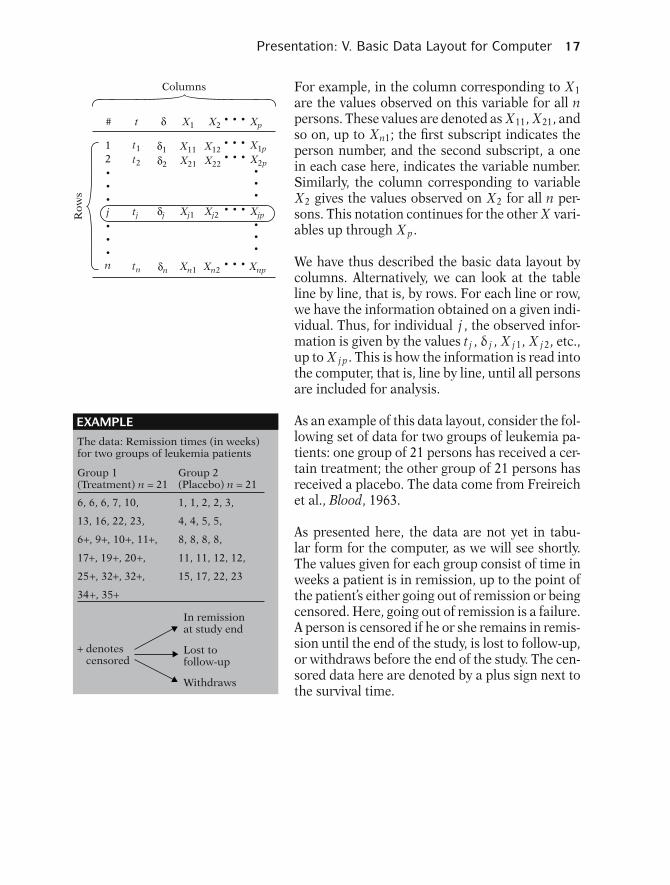
As an example of this data layout, consider the fol-lowing set of data for two groups of leukemia pa-tients: one group of 21 persons has received a cer-tain treatment; the other group of 21 persons hasreceived a placebo. The data come from Freireichet al., Blood, 1963.
As presented here, the data are not yet in tabu-lar form for the computer, as we will see shortly.The values given for each group consist of time inweeks a patient is in remission, up to the point ofthe patient’s either going out of remission or beingcensored. Here, going out of remission is a failure.A person is censored if he or she remains in remis-sion until the end of the study, is lost to follow-up,or withdraws before the end of the study. The cen-sored data here are denoted by a plus sign next tothe survival time.

18 1. Introduction to Survival Analysis
EXAMPLE (continued)
Group 1(Treatment) n = 21
Group 1
Group 2
GROUP1
# failed
9
21
1
2
3
4
5
6
7
8
9
10
11
12
13
14
15
16
17
18
19
20
21
6
6
6
7
10
13
16
22
23
6
9
10
11
17
19
20
25
32
32
34
35
1
1
1
1
1
1
1
1
1
0
0
0
0
0
0
0
0
0
0
0
0
1
1
1
1
1
1
1
1
1
1
1
1
1
1
1
1
1
1
1
1
1
Indiv.#
t(weeks)
δ(failed orcensored)
X(Group)
12
0
21
21
# censored Total
Group 2(Placebo) n = 21
6, 6, 6, 7, 10,
13, 16, 22, 23,
6+, 9+, 10+, 11+,
17+, 19+, 20+,
25+, 32+, 32+,
34+, 35+
1, 1, 2, 2, 3,
4, 4, 5, 5,
8, 8, 8, 8,
11, 11, 12, 12,
15, 17, 22, 23
Here are the data again:
Notice that the first three persons in group 1 wentout of remission at 6 weeks; the next six per-sons also went out of remission, but at failuretimes ranging from 7 to 23. All of the remain-ing persons in group 1 with pluses next to theirsurvival times are censored. For example, on linethree the first person who has a plus sign next to a6 is censored at six weeks. The remaining personsin group one are also censored, but at times rang-ing from 9 to 35 weeks.
Thus, of the 21 persons in group 1, nine failed dur-ing the study period, whereas the last 12 were cen-sored. Notice also that none of the data in group2 is censored; that is, all 21 persons in this groupwent out of remission during the study period.
We now put this data in tabular form for the com-puter, as shown at the left. The list starts with the21 persons in group 1 (listed 1–21) and follows(on the next page) with the 21 persons in group2 (listed 22–42). Our n for the composite groupis 42.
The second column of the table gives the survivaltimes in weeks for all 42 persons. The third col-umn indicates failure or censorship for each per-son. Finally, the fourth column lists the values ofthe only explanatory variable we have consideredso far, namely, group status, with 1 denoting treat-ment and 0 denoting placebo.
If we pick out any individual and read across thetable, we obtain the line of data for that person thatgets entered in the computer. For example, person#3 has a survival time of 6 weeks, and since δ = 1,this person failed, that is, went out of remission.The X value is 1 because person #3 is in group1. As a second example, person #14, who has anobserved survival time of 17 weeks, was censoredat this time because δ = 0. The X value is again 1because person #14 is also in group 1.

Presentation: VI. Basic Data Layout for Understanding Analysis 19
EXAMPLE (continued)
GROUP2
22
23
24
25
26
27
28
29
30
31
32
33
34
35
36
37
38
39
40
41
42
1
1
2
2
3
4
4
5
5
8
8
8
8
11
11
12
12
15
17
22
23
1
1
1
1
1
1
1
1
1
1
1
1
1
1
1
1
1
1
1
1
1
0
0
0
0
0
0
0
0
0
0
0
0
0
0
0
0
0
0
0
0
0
Indiv.#
t(weeks)
δ(failed orcensored)
X(Group)
As one more example, this time from group 2, per-son #32 survived 8 weeks and then failed, becauseδ = 1; the X value is 0 because person #32 is ingroup 2.
VI. Basic Data Layout forUnderstanding Analysis
We are now ready to look at another data layout,which is shown at the left. This layout helps pro-vide some understanding of how a survival analy-sis actually works and, in particular, how survivorcurves are derived.
The first column in this table gives ordered fail-ure times. These are denoted by t ’s with subscriptswithin parentheses, starting with t(0), then t(1) andso on, up to t(k). Note that the parentheses sur-rounding the subscripts distinguish ordered fail-ure times from the survival times previously givenin the computer layout.
For analysis:
t(0) = 0
t(1)
t(2)
t(k)
m0 = 0 q0
Orderedfailuretimes(t( j))
# offailures
(mj)
# censored in[t( j), t( j+1))
Riskset
R(t( j))
R(t(0))
R(t(1))
R(t(2))
R(t(k))
•
•
•
m1
m2
mk
•
•
•
q1
q2
qk
•
•
•
•
•
•
(qj)
{t1, t2, . . . , tn}
Unordered
k = # of distinct times at whick subjectsfailed (k ≤ n)
Censored t’s
Failed t’sordered (t( j))
To get ordered failure times from survival times,we must first remove from the list of unorderedsurvival times all those times that are censored; weare thus working only with those times at whichpeople failed. We then order the remaining fail-ure times from smallest to largest, and count tiesonly once. The value k gives the number of distincttimes at which subjects failed.
20 1. Introduction to Survival Analysis
EXAMPLE Remission Data: Group 1(n = 21, 9 failures, k = 7)
t(j)
t(0) = 0
t(1) = 6
t(2) = 7
t(3) = 10
t(4) = 13
t(5) = 16
t(6) = 22
t(7) = 23
Totals
(n = 21, 21 failures, k = 12)Remission Data: Group 2
9 12
mj
0
3
1
1
1
1
1
1
0
1
1
2
0
3
0
5
21 persons survive ≥ 0 wks
21 persons survive ≥ 6 wks
17 persons survive ≥ 7 wks
15 persons survive ≥ 10 wks
12 persons survive ≥ 13 wks
11 persons survive ≥ 16 wks
7 persons survive ≥ 22 wks
6 persons survive ≥ 23 wks
qj R(t( j))
t(j)
t(0) = 0
t(1) = 1
t(2) = 2
t(3) = 3
t(4) = 4
t(5) = 5
t(6) = 8
t(7) = 11
t(8) = 12
t(9) = 15
t(10) = 17
t(11) = 22
t(12) = 23
Totals 21 0
mj
0
2
2
1
2
2
4
2
2
1
1
1
1
0
0
0
0
0
0
0
0
0
0
0
0
0
21 persons survive ≥ 0 wks
21 persons survive ≥ 1 wk
19 persons survive ≥ 2 wks
17 persons survive ≥ 3 wks
16 persons survive ≥ 4 wks
14 persons survive ≥ 5 wks
12 persons survive ≥ 8 wks
8 persons survive ≥ 11 wks
6 persons survive ≥ 12 wks
4 persons survive ≥ 15 wks
3 persons survive ≥ 17 wks
2 persons survive ≥ 22 wks
1 person survive ≥ 23 wks
qj R(t( j))
ties
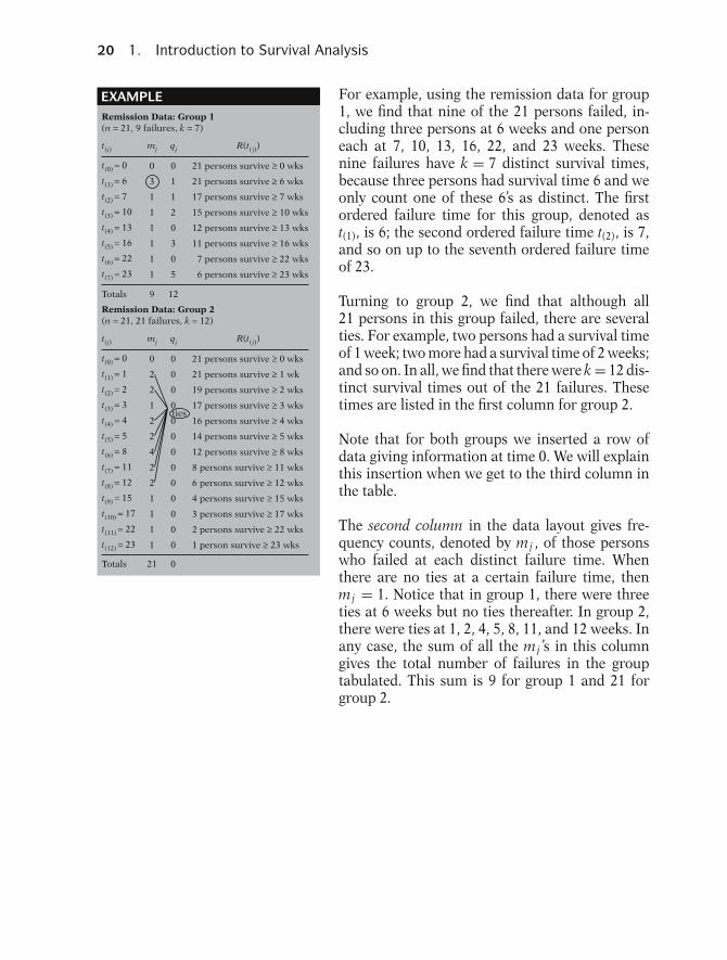
For example, using the remission data for group1, we find that nine of the 21 persons failed, in-cluding three persons at 6 weeks and one personeach at 7, 10, 13, 16, 22, and 23 weeks. Thesenine failures have k = 7 distinct survival times,because three persons had survival time 6 and weonly count one of these 6’s as distinct. The firstordered failure time for this group, denoted ast(1), is 6; the second ordered failure time t(2), is 7,and so on up to the seventh ordered failure timeof 23.
Turning to group 2, we find that although all21 persons in this group failed, there are severalties. For example, two persons had a survival timeof 1 week; two more had a survival time of 2 weeks;and so on. In all, we find that there were k = 12 dis-tinct survival times out of the 21 failures. Thesetimes are listed in the first column for group 2.
Note that for both groups we inserted a row ofdata giving information at time 0. We will explainthis insertion when we get to the third column inthe table.
The second column in the data layout gives fre-quency counts, denoted by mj , of those personswho failed at each distinct failure time. Whenthere are no ties at a certain failure time, thenmj = 1. Notice that in group 1, there were threeties at 6 weeks but no ties thereafter. In group 2,there were ties at 1, 2, 4, 5, 8, 11, and 12 weeks. Inany case, the sum of all the mj ’s in this columngives the total number of failures in the grouptabulated. This sum is 9 for group 1 and 21 forgroup 2.

Presentation: VI. Basic Data Layout for Understanding Analysis 21
EXAMPLE (continued)
Remission Data: Group 1
qj = censored in [t( j), t( j + 1))
t(j)
t(0) = 0
t(1) = 6
t(2) = 7
t(3) = 10
t(4) = 13
t(5) = 16
t(6) = 22
t(7) = 23
Totals
#
1
2
3
4
5
6
7
8
9
10
11
12
13
14
15
16
17
18
19
20
21
6
6
6
7
10
13
16
22
23
6
9
10
11
17
19
20
25
32
32
34
35
1
1
1
1
1
1
1
1
1
0
0
0
0
0
0
0
0
0
0
0
0
1
1
1
1
1
1
1
1
1
1
1
1
1
1
1
1
1
1
1
1
1
t(weeks) X(group)δ
Remission Data: Group 1
9 12
mj
0
3
1
1
1
1
1
1
0
1
1
2
0
3
0
5
21 persons survive ≥ 0 wks
21 persons survive ≥ 6 wks
17 persons survive ≥ 7 wks
15 persons survive ≥ 10 wks
12 persons survive ≥ 13 wks
11 persons survive ≥ 16 wks
7 persons survive ≥ 22 wks
6 persons survive ≥ 23 wks
qj R(t( j))
ties
The third column gives frequency counts, denotedby q j , of those persons censored in the time in-terval starting with failure time t( j ) up to the nextfailure time denoted t( j+1). Technically, because ofthe way we have defined this interval in the table,we include those persons censored at the begin-ning of the interval.
For example, the remission data, for group 1 in-cludes 5 nonzero q j ’s: q1 = 1, q2 = 1, q3 = 2 j q5 =3, q7 = 5. Adding these values gives us the to-tal number of censored observations for group 1,which is 12. Moreover, if we add the total numberof q ’s (12) to the total number of m’s (9), we get thetotal number of subjects in group 1, which is 21.
We now focus on group 1 to look a little closerat the q ’s. At the left, we list the unordered group1 information followed (on the next page) by theordered failure time information. We will go backand forth between these two tables (and pages) aswe discuss the q ’s. Notice that in the table here,one person, listed as #10, was censored at week 6.Consequently, in the table at the top of the nextpage, we have q1 = 1, which is listed on the sec-ond line corresponding to the ordered failure timet(1), which equals 6.
The next q is a little trickier, it is derived from theperson who was listed as #11 in the table here andwas censored at week 9. Correspondingly, in thetable at the top of the next page, we have q2 = 1because this one person was censored within thetime interval that starts at the second ordered fail-ure time, 7 weeks, and ends just before the third or-dered failure time, 10 weeks. We have not countedhere person #12, who was censored at week 10,because this person’s censored time is exactly atthe end of the interval. We count this person inthe following interval.
22 1. Introduction to Survival Analysis
EXAMPLE (continued)Group 1 using ordered failure times
t(j)
t(1) = 6
t(2) = 7
t(3) = 10
t(4) = 13
t(5) = 16
t(6) = 22
t(7) = 23
Totals 9 12
mj
3
1
1
1
1
1
1
1
1
2
0
3
0
5
21 persons survive ≥ 6 wks
17 persons survive ≥ 7 wks
15 persons survive ≥ 10 wks
12 persons survive ≥ 13 wks
11 persons survive ≥ 16 wks
7 persons survive ≥ 22 wks
6 persons survive ≥ 23 wks
qj R(t( j))
t(0) = 0 0 0 21 persons survive ≥ 0 wks
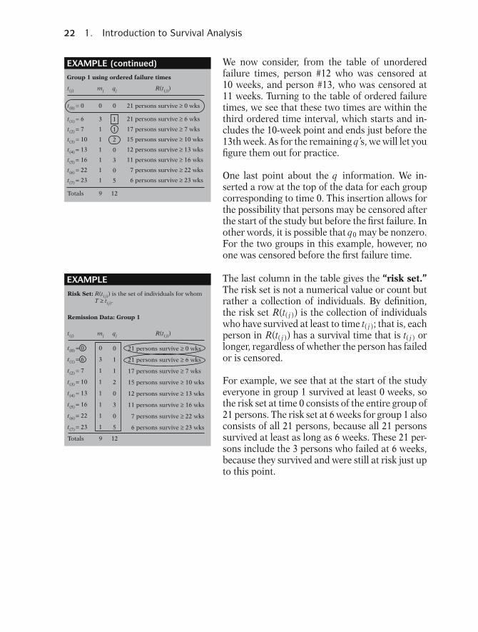
We now consider, from the table of unorderedfailure times, person #12 who was censored at10 weeks, and person #13, who was censored at11 weeks. Turning to the table of ordered failuretimes, we see that these two times are within thethird ordered time interval, which starts and in-cludes the 10-week point and ends just before the13th week. As for the remaining q ’s, we will let youfigure them out for practice.
One last point about the q information. We in-serted a row at the top of the data for each groupcorresponding to time 0. This insertion allows forthe possibility that persons may be censored afterthe start of the study but before the first failure. Inother words, it is possible that q0 may be nonzero.For the two groups in this example, however, noone was censored before the first failure time.
EXAMPLE
Risk Set: R(t( j)) is the set of individuals for whom
Remission Data: Group 1
t(0) = 0
t(1) = 6
t(2) = 7
t(3) = 10
t(4) = 13
t(5) = 16
t(6) = 22
t(7) = 23
0
3
1
1
1
1
1
1
0
1
1
2
0
3
0
5
21 persons survive ≥ 0 wks
21 persons survive ≥ 6 wks
17 persons survive ≥ 7 wks
15 persons survive ≥ 10 wks
12 persons survive ≥ 13 wks
11 persons survive ≥ 16 wks
7 persons survive ≥ 22 wks
6 persons survive ≥ 23 wks
t(j) mj qj R(t( j))
Totals 9 12
T ≥ t(j).
The last column in the table gives the “risk set.”The risk set is not a numerical value or count butrather a collection of individuals. By definition,the risk set R(t( j )) is the collection of individualswho have survived at least to time t( j ); that is, eachperson in R(t( j )) has a survival time that is t( j ) orlonger, regardless of whether the person has failedor is censored.
For example, we see that at the start of the studyeveryone in group 1 survived at least 0 weeks, sothe risk set at time 0 consists of the entire group of21 persons. The risk set at 6 weeks for group 1 alsoconsists of all 21 persons, because all 21 personssurvived at least as long as 6 weeks. These 21 per-sons include the 3 persons who failed at 6 weeks,because they survived and were still at risk just upto this point.

Presentation: VI. Basic Data Layout for Understanding Analysis 23
EXAMPLE (continued)
t(0) = 0
t(1) = 6
t(2) = 7
t(3) = 10
t(4) = 13
t(5) = 16
t(6) = 22
t(7) = 23
0
3
1
1
1
1
1
1
0
1
1
2
0
3
0
5
21 persons survive ≥ 0 wks
21 persons survive ≥ 6 wks
17 persons survive ≥ 7 wks
15 persons survive ≥ 10 wks
12 persons survive ≥ 13 wks
11 persons survive ≥ 16 wks
7 persons survive ≥ 22 wks
6 persons survive ≥ 23 wks
t(j) mj qj R(t( j))
Totals 9 12
t(0) = 0
t(1) = 6
t(2) = 7
t(3) = 10
t(4) = 13
t(5) = 16
t(6) = 22
t(7) = 23
0
3
1
1
1
1
1
1
0
1
1
2
0
3
0
5
21 persons survive ≥ 0 wks
21 persons survive ≥ 6 wks
17 persons survive ≥ 7 wks
15 persons survive ≥ 10 wks
12 persons survive ≥ 13 wks
11 persons survive ≥ 16 wks
7 persons survive ≥ 22 wks
6 persons survive ≥ 23 wks
Totals 9 12
Now let’s look at the risk set at 7 weeks. This setconsists of seventeen persons in group 1 that sur-vived at least 7 weeks. We omit everyone in theX-ed area. Of the original 21 persons, we there-fore have excluded the three persons who failedat 6 weeks and the one person who was censoredat 6 weeks. These four persons did not survive atleast 7 weeks. Although the censored person mayhave survived longer than 7 weeks, we must ex-clude him or her from the risk set at 7 weeks be-cause we have information on this person only upto 6 weeks.
To derive the other risk sets, we must excludeall persons who either failed or were censoredbefore the start of the time interval being con-sidered. For example, to obtain the risk set at13 weeks for group 1, we must exclude the fivepersons who failed before, but not including,13 weeks and the four persons who were censoredbefore, but not including, 13 weeks. Subtractingthese nine persons from 21, leaves twelve personsin group 1 still at risk for getting the event at13 weeks. Thus, the risk set consists of these twelvepersons.
How we work with censored data:Use all informaton up to time of cen-sorship; don’t throw away informa-tion.
The importance of the table of ordered failuretimes is that we can work with censored obser-vations in analyzing survival data. Even thoughcensored observations are incomplete, in that wedon’t know a person’s survival time exactly, we canstill make use of the information we have on acensored person up to the time we lose track ofhim or her. Rather than simply throw away theinformation on a censored person, we use all theinformation we have on such a person up untiltime of censorship. (Nevertheless, most survivalanalysis techniques require a key assumption thatcensoring is non-informative—censored subjectsare not at increased risk for failure. See Chapter 9on competing risks for further details.)
24 1. Introduction to Survival Analysis
EXAMPLE
t(j)
6
7
10
13
16
22
23
mj
3
1
1
1
1
1
1
1
1
2
0
3
0
5
21 persons
17 persons
15 persons
12 persons
11 persons
7 persons
6 persons
qj R(t( j))
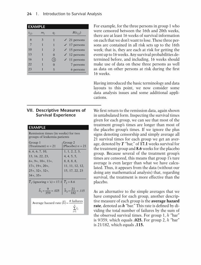
For example, for the three persons in group 1 whowere censored between the 16th and 20th weeks,there are at least 16 weeks of survival informationon each that we don’t want to lose. These three per-sons are contained in all risk sets up to the 16thweek; that is, they are each at risk for getting theevent up to 16 weeks. Any survival probabilities de-termined before, and including, 16 weeks shouldmake use of data on these three persons as wellas data on other persons at risk during the first16 weeks.
Having introduced the basic terminology and datalayouts to this point, we now consider somedata analysis issues and some additional appli-cations.
VII. Descriptive Measures ofSurvival Experience
EXAMPLE
Remission times (in weeks) for twogroups of leukemia patients
Group 1(Treatment) n = 21
6, 6, 6, 7, 10,
13, 16, 22, 23,
6+, 9+, 10+, 11+,
17+, 19+, 20+,
25+, 32+, 32+,
34+, 35+
1, 1, 2, 2, 3,
4, 4, 5, 5,
8, 8, 8, 8,
11, 11, 12, 12,
15, 17, 22, 23
Group 2(Placebo) n = 21
T1 (ignoring + ’s) = 17.1 T2 = 8.6
h1 = 9359
= .025 h2 = 21182
= .115
# failuresAverage hazard rate (h) =
n
i=1ti∑
We first return to the remission data, again shownin untabulated form. Inspecting the survival timesgiven for each group, we can see that most of thetreatment group’s times are longer than most ofthe placebo group’s times. If we ignore the plussigns denoting censorship and simply average all21 survival times for each group we get an aver-age, denoted by T “bar,” of 17.1 weeks survival forthe treatment group and 8.6 weeks for the placebogroup. Because several of the treatment group’stimes are censored, this means that group 1’s tureaverage is even larger than what we have calcu-lated. Thus, it appears from the data (without ourdoing any mathematical analysis) that, regardingsurvival, the treatment is more effective than theplacebo.
As an alternative to the simple averages that wehave computed for each group, another descrip-tive measure of each group is the average hazardrate, denoted as h “bar.” This rate is defined by di-viding the total number of failures by the sum ofthe observed survival times. For group 1, h “bar”is 9/359, which equals .025. For group 2, h “bar”is 21/182, which equals .115.
Presentation: VII. Descriptive Measures of Survival Experience 25
h
s As previously described, the hazard rate indicatesfailure potential rather than survival probability.Thus, the higher the average hazard rate, the loweris the group’s probability of surviving.
In our example, the average hazard for the treat-ment group is smaller than the average hazard forthe placebo group.
Placebo hazard > treatment hazard:suggests that treatment is moreeffective than placebo
Thus, using average hazard rates, we again see thatthe treatment group appears to be doing betteroverall than the placebo group; that is, the treat-ment group is less prone to fail than the placebogroup.
Descriptive measures (T and h) giveoverall comparison; they do notgive comparison over time.
The descriptive measures we have used so far—theordinary average and the hazard rate average—provide overall comparisons of the treatmentgroup with the placebo group. These measuresdon’t compare the two groups at different points intime of follow-up. Such a comparison is providedby a graph of survivor curves.
Median = 8 Median = 23
0
.5
1
10 20t weeks
Group 2 placebo
Group 1 treatment
S(t)
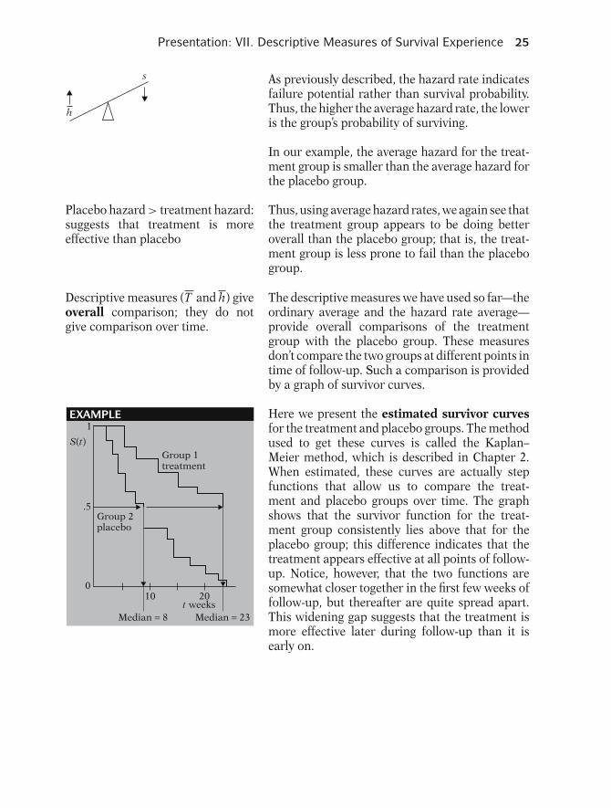
EXAMPLE Here we present the estimated survivor curvesfor the treatment and placebo groups. The methodused to get these curves is called the Kaplan–Meier method, which is described in Chapter 2.When estimated, these curves are actually stepfunctions that allow us to compare the treat-ment and placebo groups over time. The graphshows that the survivor function for the treat-ment group consistently lies above that for theplacebo group; this difference indicates that thetreatment appears effective at all points of follow-up. Notice, however, that the two functions aresomewhat closer together in the first few weeks offollow-up, but thereafter are quite spread apart.This widening gap suggests that the treatment ismore effective later during follow-up than it isearly on.

26 1. Introduction to Survival Analysis
0.5
0
1
Median X
Y
Median (treatment) = 23 weeksMedian (placebo) = 8 weeks
Also notice from the graph that one can obtainestimates of the median survival time, the time atwhich the survival probability is .5 for each group.Graphically, the median is obtained by proceedinghorizontally from the 0.5 point on the Y -axis un-til the survivor curve is reached, as marked by anarrow, and then proceeding vertically downwarduntil the X -axis is crossed at the median survivaltime.
For the treatment group, the median is 23 weeks;for the placebo group, the median is 8 weeks. Com-parison of the two medians reinforces our previ-ous observation that the treatment is more effec-tive overall than the placebo.
VIII. Example: ExtendedRemission Data
Group 1
6 2.31
6 4.06
6 3.28
7 4.43
10 2.96
13 2.88
16 3.60
22 2.32
23 2.57
6+ 3.20
9+ 2.80
10+ 2.70
11+ 2.60
17+ 2.16
19+ 2.05
20+ 2.01
25+ 1.78
32+ 2.20
32+ 2.53
34+ 1.47
35+ 1.45
1 2.80
1 5.00
2 4.91
2 4.48
3 4.01
4 4.36
4 2.42
5 3.49
5 3.97
8 3.52
8 3.05
8 2.32
8 3.26
11 3.49
11 2.12
12 1.50
12 3.06
15 2.30
17 2.95
22 2.73
23 1.97
log WBCt (weeks)
Group 2
log WBCt (weeks)
Before proceeding to another data set, we con-sider the remission example data (Freireich et al.,Blood, 1963) in an extended form. The table at theleft gives the remission survival times for the twogroups with additional information about whiteblood cell count for each person studied. In par-ticular, each person’s log white blood cell countis given next to that person’s survival time. Theepidemiologic reason for adding log WBC to thedata set is that this variable is usually consideredan important predictor of survival in leukemia pa-tients; the higher the WBC, the worse the prog-nosis. Thus, any comparison of the effects of twotreatment groups needs to consider the possibleconfounding effect of such a variable.

Presentation: VIII. Example: Extended Remission Data 27
Treatment group: log WBC = 1.8Placebo group: log WBC = 4.1Indicates confounding of treatmenteffect by log WBC
PlaceboTreatment
Frequencydistribution
log WBC
EXAMPLE: CONFOUNDING
Need to adjust for imbalance in thedistribution of log WBC
Although a full exposition of the nature of con-founding is not intended here, we provide a sim-ple scenario to give you the basic idea. Supposeall of the subjects in the treatment group had verylow log WBC, with an average, for example, of 1.8,whereas all of the subjects in the placebo grouphad very high log WBC, with an average of 4.1.We would have to conclude that the results we’veseen so far that compare treatment with placebogroups may be misleading.
The additional information on log WBC wouldsuggest that the treatment group is survivinglonger simply because of their low WBC and notbecause of the efficacy of the treatment itself. Inthis case, we would say that the treatment effectis confounded by the effect of log WBC.
More typically, the distribution of log WBC may bequite different in the treatment group than in thecontrol group. We have illustrated one extreme inthe graph at the left. Even though such an extremeis not likely, and is not true for the data given here,the point is that some attempt needs to be made toadjust for whatever imbalance there is in the dis-tribution of log WBC. However, if high log WBCcount was a consequence of the treatment, thenwhite blood cell count should not be controlledfor in the analysis.
Treatment by log WBC interaction
High log WBC Low log WBC
Placebo Placebo
S(t) S(t)
Treatment
Treatment
t t
EXAMPLE: INTERACTION Another issue to consider regarding the effect oflog WBC is interaction. What we mean by inter-action is that the effect of the treatment may bedifferent, depending on the level of log WBC. Forexample, suppose that for persons with high logWBC, survival probabilities for the treatment areconsistently higher over time than for the placebo.This circumstance is illustrated by the first graphat the left. In contrast, the second graph, whichconsiders only persons with low log WBC, showsno difference in treatment and placebo effect overtime. In such a situation, we would say that thereis strong treatment by log WBC interaction, andwe would have to qualify the effect of the treat-ment as depending on the level of log WBC.
28 1. Introduction to Survival Analysis
Need to consider:
� interaction;� confounding.
The example of interaction we just gave is but oneway interaction can occur; on the other hand, in-teraction may not occur at all. As with confound-ing, it is beyond our scope to provide a thoroughdiscussion of interaction. In any case, the assess-ment of interaction is something to consider inone’s analysis in addition to confounding that in-volves explanatory variables.
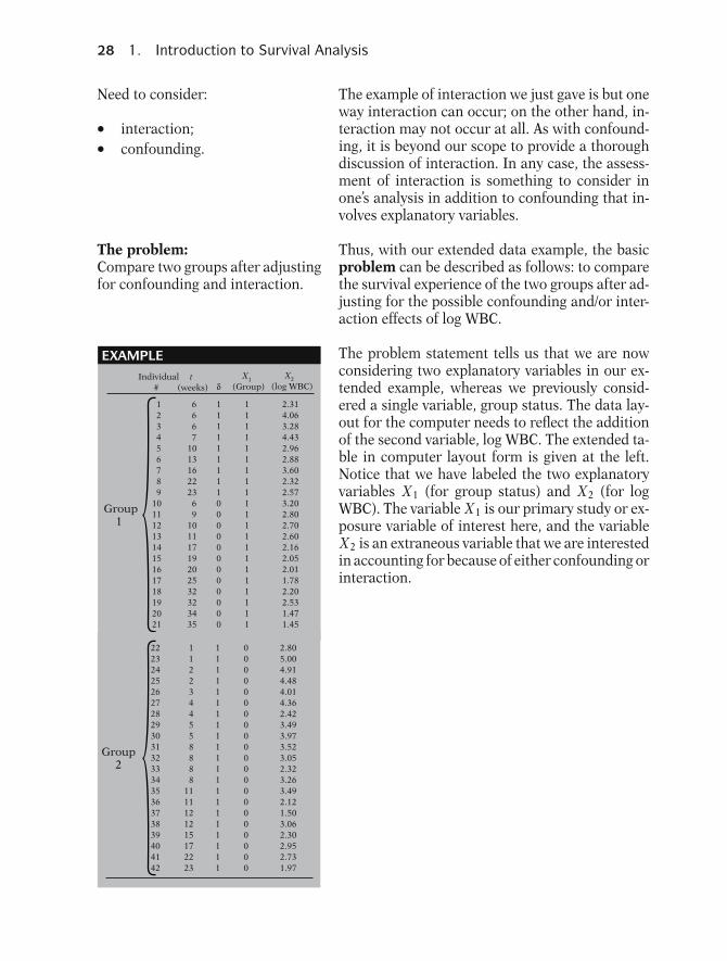
The problem:Compare two groups after adjustingfor confounding and interaction.
Thus, with our extended data example, the basicproblem can be described as follows: to comparethe survival experience of the two groups after ad-justing for the possible confounding and/or inter-action effects of log WBC.
EXAMPLE
Group1
123456789
101112131415161718192021
6667
101316222369
10111719202532323435
111111111000000000000
111111111111111111111
2.314.063.284.432.962.883.602.322.573.202.802.702.602.162.052.011.782.202.531.471.45
Individual#
t(weeks) δ
X2(log WBC)
X1(Group)
Group2
222324252627282930313233343536373839404142
1122344558888
1111121215172223
111111111111111111111
000000000000000000000
2.805.004.914.484.014.362.423.493.973.523.052.323.263.492.121.503.062.302.952.731.97
The problem statement tells us that we are nowconsidering two explanatory variables in our ex-tended example, whereas we previously consid-ered a single variable, group status. The data lay-out for the computer needs to reflect the additionof the second variable, log WBC. The extended ta-ble in computer layout form is given at the left.Notice that we have labeled the two explanatoryvariables X1 (for group status) and X2 (for logWBC). The variable X1 is our primary study or ex-posure variable of interest here, and the variableX2 is an extraneous variable that we are interestedin accounting for because of either confounding orinteraction.

Presentation: IX. Multivariable Example 29
Analysis alternatives:
� stratify on log WBC;� use math modeling, e.g.,proportional hazards model.
As implied by our extended example, which con-siders the possible confounding or interaction ef-fect of log WBC, we need to consider methods foradjusting for log WBC and/or assessing its effect inaddition to assessing the effect of treatment group.The two most popular alternatives for analysis arethe following:
� to stratify on log WBC and compare survivalcurves for different strata; or� to use mathematical modeling proceduressuch as the proportional hazards or other sur-vival models; such methods will be describedin subsequent chapters.
IX. Multivariable Example We now consider one other example. Our purposehere is to describe a more general type of mul-tivariable survival analysis problem. The readermay see the analogy of this example to multipleregression or even logistic regression data prob-lems.
� Describes general multivariablesurvival problem.� Gives analogy to regressionproblems.
EXAMPLE
13-year follow-up of fixed cohort fromEvans County, Georgia
n = 170 white males (60+)
T = years until deathEvent = death
Explanatory variables:
Exposure:Social Network Index (SNI)
Absenceof socialnetwork
Excellentsocial
network
0 1 2 3 4 5
• exposure variable• confounders• interaction variables
We consider a data set developed from a 13-yearfollow up study of a fixed cohort of persons inEvans County Georgia, during the period 1967–1980 (Schoenbach et al., Amer. J. Epid., 1986).From this data set, we focus or a portion contain-ing n = 170 white males who are age 60 or olderat the start of follow-up in 1967.
For this data set, the outcome variable is T , timein years until death from start of follow-up, sothe event of interest is death. Several explanatoryvariables are measured, one of which is consideredthe primary exposure variable; the other variablesare considered as potential confounders and/or in-teraction variables.
The primary exposure variable is a measure calledSocial Network Index (SNI). This is an ordinalvariable derived from questionnaire measurementand is designed to assess the extent to which astudy subject has social contacts of various types.With the questionnaire, a scale is used with valuesranging from 0 (absence of any social network) to5 (excellent social network).

30 1. Introduction to Survival Analysis
EXAMPLE (continued)
The problem:
Goals:• Measure of effect (adjusted)
• Decide on variables to be adjusted; determine method of adjustment
• Survivor curves for different SNIcategories (adjusted)
To describe the relationship betweenSNI and time to death, aftercontrolling for AGE, SBP, CHR,QUET, and SOCL.
SNIAGESBPCHRQUETSOCL
Explanatory variables:
Exposure variable
Potential confounders/interaction variables
Note : QUET = weight
(height)2× 100
Study goal: to determine whether SNI isprotective against death,i.e., SNI ⇒ S(t)→ →
The study’s goal is to determine whether one’ssocial network, as measured by SNI, is protec-tive against death. If this study hypothesis is cor-rect, then the higher the social network score, thelonger will be one’s survival time.
In evaluating this problem, several explanatoryvariables, in addition to SNI, are measured at thestart of follow-up. These include AGE, systolicblood pressure (SBP), an indicator of the presenceor absence of some chronic disease (CHR), bodysize as measured by Quetelet’s index (QUET =weight over height squared times 100), and socialclass (SOCL).
These five additional variables are of interest be-cause they are thought to have their own specialor collective influence on how long a person willsurvive. Consequently, these variables are viewedas potential confounders and/or interaction vari-ables in evaluating the effect of social network ontime to death.
We can now clearly state the problem being ad-dressed by this study: To describe the relationshipbetween SNI and time to death, controlling forAGE, SBP, CHR, QUET, and SOCL.
Our goals in using survival analysis to solve thisproblem are as follows:
� to obtain some measure of effect that will de-scribe the relationship between SNI and timeuntil death, after adjusting for the other vari-ables we have identified;� to develop survival curves that describe theprobability of survival over time for differentcategories of social networks; in particular, wewish to compare the survival of persons withexcellent networks to the survival of personswith poor networks. Such survival curves needto be adjusted for the effects of other variables.� to achieve these goals, two intermediary goalsare to decide which of the additional variablesbeing considered need to be adjusted and todetermine an appropriate method of adjust-ment.

Presentation: X. Math Models in Survival Analysis 31
The computer data layout for this problem is givenbelow. The first column lists the 170 individualsin the data set. The second column lists the sur-vival times, and the third column lists failure orcensored status. The remainder of the columnslist the 6 explanatory variables of interest, start-ing with the exposure variable SNI and continu-ing with the variables to be accounted for in theanalysis.
Computer layout: 13-year follow-up study (1967–1980) of a fixed cohort of n = 170white males (60+) from Evans County, Georgia
# t δ SNI AGE SBP CHR QUET SOCL
1 t1 δ1 SNI1 AGE1 SBP1 CHR1 QUET1 SOCL12 t2 δ2 SNI2 AGE2 SBP2 CHR2 QUET2 SOCL2. . . . . . . . .. . . . . . . . .. . . . . . . . .
170 t170 δ170 SNI170 AGE170 SBP170 CHR170 QUET170 SOCL170
X. Math Models in SurvivalAnalysis
It is beyond the scope of this presentation to pro-vide specific details of the survival analysis ofthese data. Nevertheless, the problem addressedby these data is closely analogous to the typicalmultivariable problem addressed by linear and lo-gistic regression modeling. Regardless of whichmodeling approach is chosen, the typical problemconcerns describing the relationship between anexposure variable (e.g., E) and an outcome vari-able (e.g., D) after controlling for the possible con-founding and interaction effects of additional vari-ables (e.g., C1, C2, and so on up to Cp). In oursurvival analysis example, E is the social networkvariable SNI, D is the survival time variable, andthere are p = 5 C variables, namely, AGE, SBP,CHR, QUET, and SOCL.
General framework
E D
Controlling for C1, C2, . . . Cp.
SNI study:
Controlling for AGE, SBP, CHR,QUET, and SOCL
E = SNI D = survival time
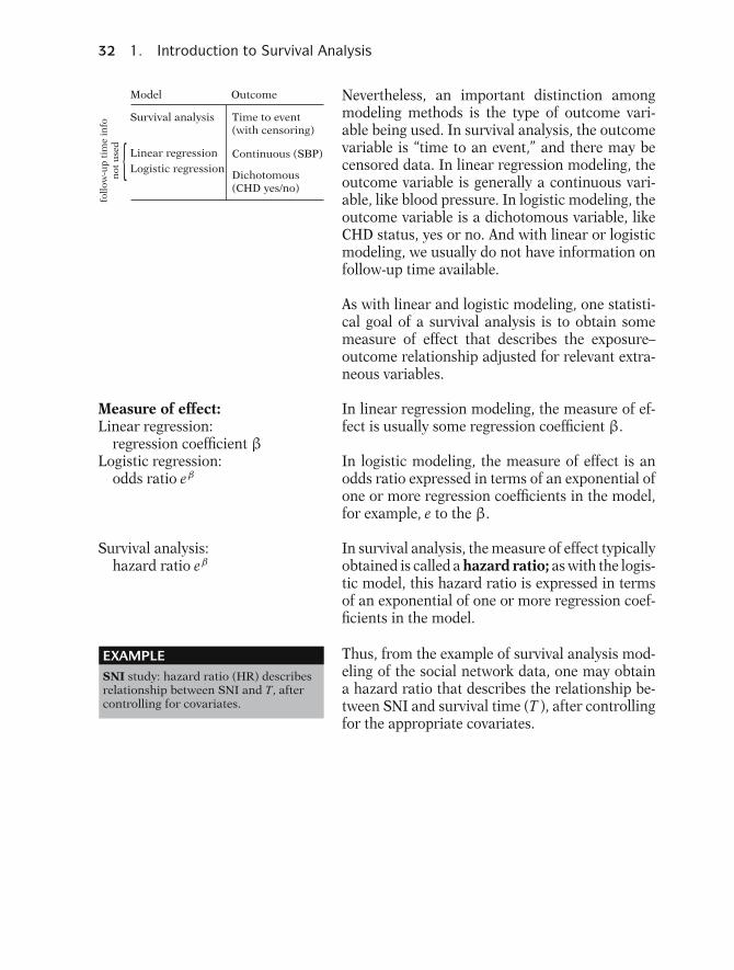
32 1. Introduction to Survival Analysis
Model Outcome
Time to event (with censoring)
Continuous (SBP)
Dichotomous(CHD yes/no)
Survival analysis
Linear regression
Logistic regression{
foll
ow-u
p t
ime
info
n
ot u
sed
Nevertheless, an important distinction amongmodeling methods is the type of outcome vari-able being used. In survival analysis, the outcomevariable is “time to an event,” and there may becensored data. In linear regression modeling, theoutcome variable is generally a continuous vari-able, like blood pressure. In logistic modeling, theoutcome variable is a dichotomous variable, likeCHD status, yes or no. And with linear or logisticmodeling, we usually do not have information onfollow-up time available.
As with linear and logistic modeling, one statisti-cal goal of a survival analysis is to obtain somemeasure of effect that describes the exposure–outcome relationship adjusted for relevant extra-neous variables.
Measure of effect:Linear regression:
regression coefficient βLogistic regression:
odds ratio eβ
In linear regression modeling, the measure of ef-fect is usually some regression coefficient β.
In logistic modeling, the measure of effect is anodds ratio expressed in terms of an exponential ofone or more regression coefficients in the model,for example, e to the β.
Survival analysis:hazard ratio eβ
In survival analysis, the measure of effect typicallyobtained is called a hazard ratio; as with the logis-tic model, this hazard ratio is expressed in termsof an exponential of one or more regression coef-ficients in the model.
EXAMPLESNI study: hazard ratio (HR) describesrelationship between SNI and T, aftercontrolling for covariates.
Thus, from the example of survival analysis mod-eling of the social network data, one may obtaina hazard ratio that describes the relationship be-tween SNI and survival time (T ), after controllingfor the appropriate covariates.
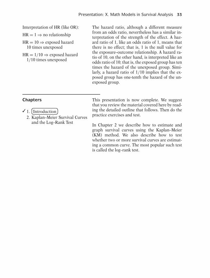
Presentation: X. Math Models in Survival Analysis 33
Interpretation of HR (like OR):
HR = 1 ⇒ no relationship
HR = 10 ⇒ exposed hazard10 times unexposed
HR = 1/10 ⇒ exposed hazard1/10 times unexposed
The hazard ratio, although a different measurefrom an odds ratio, nevertheless has a similar in-terpretation of the strength of the effect. A haz-ard ratio of 1, like an odds ratio of 1, means thatthere is no effect; that is, 1 is the null value forthe exposure–outcome relationship. A hazard ra-tio of 10, on the other hand, is interpreted like anodds ratio of 10; that is, the exposed group has tentimes the hazard of the unexposed group. Simi-larly, a hazard ratio of 1/10 implies that the ex-posed group has one-tenth the hazard of the un-exposed group.
Chapters This presentation is now complete. We suggestthat you review the material covered here by read-ing the detailed outline that follows. Then do thepractice exercises and test.
✓ 1.�
�
�
�Introduction2. Kaplan–Meier Survival Curves
and the Log–Rank TestIn Chapter 2 we describe how to estimate andgraph survival curves using the Kaplan–Meier(KM) method. We also describe how to testwhether two or more survival curves are estimat-ing a common curve. The most popular such testis called the log–rank test.

34 1. Introduction to Survival Analysis
DetailedOutline
I. What is survival analysis? (pages 4–5)A. Type of problem addressed: outcome variable is
time until an event occurs.B. Assume one event of interest; more than one type
of event implies a competing risk problem.C. Terminology: time = survival time; event = failure.D. Examples of survival analysis:
i. leukemia patients/time in remissionii. disease-free cohort/time until heart disease
iii. elderly population/time until deathiv. parolees/time until rearrest (recidivism)v. heart transplants/time until death
II. Censored data (pages 5–8)A. Definition: don’t know exact survival time.B. Reasons: study ends without subject getting event;
lost to follow-up; withdraws.C. Examples of survival data for different persons;
summary table.III. Terminology and notation (pages 8–14)
A. Notation: T = survival time random variable:t = specific value for Tδ = (0–1) variable for failure/censorship
statusB. Terminology: S(t) = survivor function
h(t) = hazard functionC. Properties of survivor function:� theoretically, graph is smooth curve, decreasing
from S(t) = 1 at time t = 0 to S(t) = 0 at t = ∞;� in practice, graph is step function that may notgo all the way to zero at end of study if noteveryone studied gets the event.
D. Hazard function formula:
h(t) = lim�t→0
P (t ≤ T < t + �t|T ≥ t)�t
E. Hazard function properties:� h(t) gives instantaneous potential for event tooccur given survival up to time t;� instantaneous potential idea is illustrated byvelocity;� hazard function also called “conditional failurerate”;� h(t) ≥ 0; has no upper bound; not a probability;depends on time units.
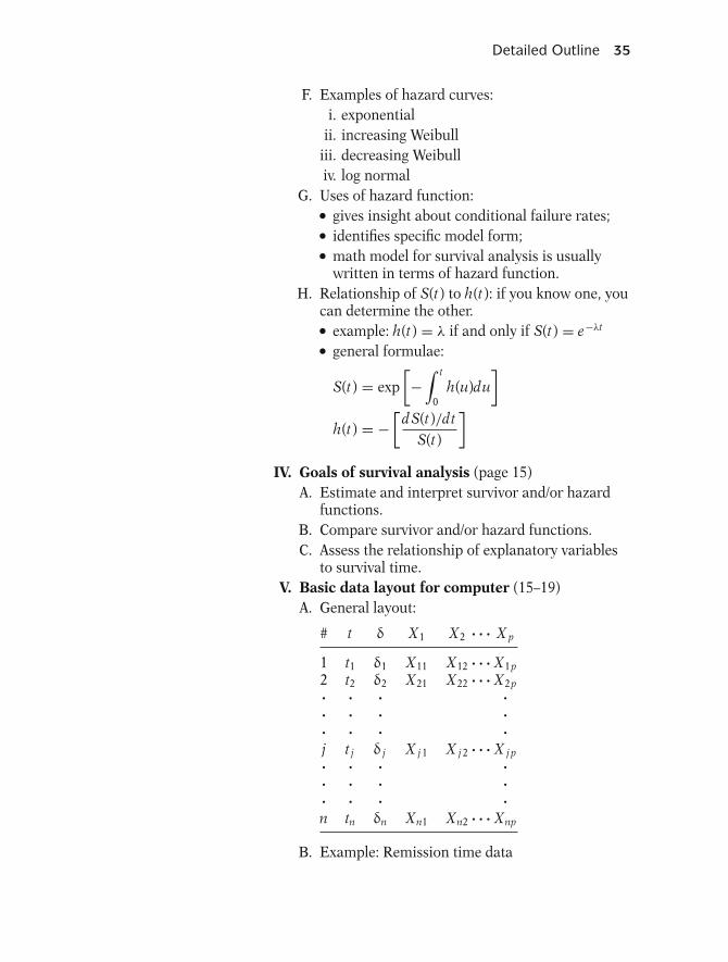
Detailed Outline 35
F. Examples of hazard curves:i. exponential
ii. increasing Weibulliii. decreasing Weibulliv. log normal
G. Uses of hazard function:� gives insight about conditional failure rates;� identifies specific model form;� math model for survival analysis is usuallywritten in terms of hazard function.
H. Relationship of S(t) to h(t): if you know one, youcan determine the other.� example: h(t) = λ if and only if S(t) = e−λt
� general formulae:
S(t) = exp[−
∫ t
0h(u)du
]h(t) = −
[d S(t)/dt
S(t)
]IV. Goals of survival analysis (page 15)
A. Estimate and interpret survivor and/or hazardfunctions.
B. Compare survivor and/or hazard functions.C. Assess the relationship of explanatory variables
to survival time.V. Basic data layout for computer (15–19)
A. General layout:
# t δ X1 X2 · · · X p
1 t1 δ1 X11 X12 · · · X1p2 t2 δ2 X21 X22 · · · X2p· · · ·· · · ·· · · ·j t j δ j X j 1 X j 2 · · · X j p· · · ·· · · ·· · · ·n tn δn Xn1 Xn2 · · · Xnp
B. Example: Remission time data
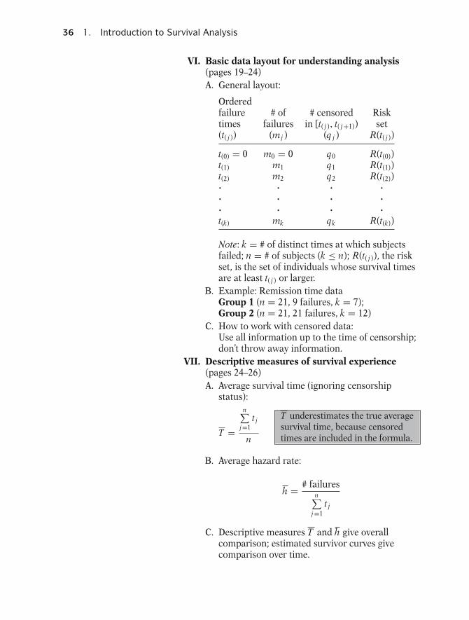
36 1. Introduction to Survival Analysis
VI. Basic data layout for understanding analysis(pages 19–24)A. General layout:
Orderedfailure # of # censored Risktimes failures in [t( j ), t( j+1)) set(t( j )) (mj ) (q j ) R(t( j ))
t(0) = 0 m0 = 0 q0 R(t(0))t(1) m1 q1 R(t(1))t(2) m2 q2 R(t(2))· · · ·· · · ·· · · ·t(k) mk qk R(t(k))
Note: k = # of distinct times at which subjectsfailed; n = # of subjects (k ≤ n); R(t( j )), the riskset, is the set of individuals whose survival timesare at least t( j ) or larger.
B. Example: Remission time dataGroup 1 (n = 21, 9 failures, k = 7);Group 2 (n = 21, 21 failures, k = 12)
C. How to work with censored data:Use all information up to the time of censorship;don’t throw away information.
VII. Descriptive measures of survival experience(pages 24–26)A. Average survival time (ignoring censorship
status):
T =
n∑j=1
t j
n
T underestimates the true averagesurvival time, because censoredtimes are included in the formula.
B. Average hazard rate:
h = # failuresn∑
j=1t j
C. Descriptive measures T and h give overallcomparison; estimated survivor curves givecomparison over time.
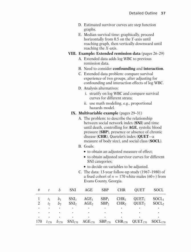
Detailed Outline 37
D. Estimated survivor curves are step functiongraphs.
E. Median survival time: graphically, proceedhorizontally from 0.5 on the Y -axis untilreaching graph, then vertically downward untilreaching the X -axis.
VIII. Example: Extended remission data (pages 26–29)A. Extended data adds log WBC to previous
remission data.B. Need to consider confounding and interaction.C. Extended data problem: compare survival
experience of two groups, after adjusting forconfounding and interaction effects of log WBC.
D. Analysis alternatives:i. stratify on log WBC and compare survival
curves for different strata;ii. use math modeling, e.g., proportional
hazards model.IX. Multivariable example (pages 29–31)
A. The problem: to describe the relationshipbetween social network index (SNI) and timeuntil death, controlling for AGE, systolic bloodpressure (SBP), presence or absence of chronicdisease (CHR), Quetelet’s index (QUET—ameasure of body size), and social class (SOCL).
B. Goals:� to obtain an adjusted measure of effect;� to obtain adjusted survivor curves for differentSNI categories;� to decide on variables to be adjusted.
C. The data: 13-year follow-up study (1967–1980) ofa fixed cohort of n = 170 white males (60+) fromEvans County, Georgia.
# t δ SNI AGE SBP CHR QUET SOCL
1 t1 δ1 SNI1 AGE1 SBP1 CHR1 QUET1 SOCL12 t2 δ2 SNI2 AGE2 SBP2 CHR2 QUET2 SOCL2· · · · · · · · ·· · · · · · · · ·· · · · · · · · ·
170 t170 δ170 SNI170 AGE170 SBP170 CHR170 QUET170 SOCL170
38 1. Introduction to Survival Analysis
X. Math models in survival analysis (pages 31–33)A. Survival analysis problem is analogous to typical
multivariable problem addressed by linearand/or logistic regression modeling: describerelationship of exposure to outcome, afteraccounting for possible confounding andinteraction.
B. Outcome variable (time to event) for survivalanalysis is different from linear (continuous) orlogistic (dichotomous) modeling.
C. Measure of effect typically used in survivalanalysis: hazard ratio (HR).
D. Interpretation of HR: like OR. SNI study: HRdescribes relationship between SNI and T , aftercontrolling for covariates.
PracticeExercises
True or False (Circle T or F):
T F 1. In a survival analysis, the outcome variable is di-chotomous.
T F 2. In a survival analysis, the event is usually de-scribed by a (0,1) variable.
T F 3. If the study ends before an individual has gottenthe event, then his or her survival time is censored.
T F 4. If, for a given individual, the event occurs beforethe person is lost to follow-up or withdraws fromthe study, then this person’s survival time is cen-sored.
T F 5. S(t) = P (T > t) is called the hazard function.T F 6. The hazard function is a probability.T F 7. Theoretically, the graph of a survivor function is
a smooth curve that decreases from S(t) = 1 att = 0 to S(t) = 0 at t = ∞.
T F 8. The survivor function at time t gives the instanta-neous potential per unit time for a failure to occur,given survival up to time t.
T F 9. The formula for a hazard function involves a con-ditional probability as one of its components.
T F 10. The hazard function theoretically has no upperbound.
T F 11. Mathematical models for survival analysis are fre-quently written in terms of a hazard function.
T F 12. One goal of a survival analysis is to compare sur-vivor and/or hazard functions.
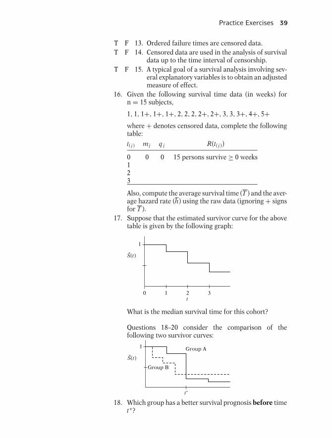
Practice Exercises 39
T F 13. Ordered failure times are censored data.T F 14. Censored data are used in the analysis of survival
data up to the time interval of censorship.T F 15. A typical goal of a survival analysis involving sev-
eral explanatory variables is to obtain an adjustedmeasure of effect.
16. Given the following survival time data (in weeks) forn = 15 subjects,
1, 1, 1+, 1+, 1+, 2, 2, 2, 2+, 2+, 3, 3, 3+, 4+, 5+where + denotes censored data, complete the followingtable:
t( j ) mj q j R(t( j ))
0 0 0 15 persons survive ≥ 0 weeks123
Also, compute the average survival time (T ) and the aver-age hazard rate (h) using the raw data (ignoring + signsfor T ).
17. Suppose that the estimated survivor curve for the abovetable is given by the following graph:
1
1
20 3
S(t)
t
What is the median survival time for this cohort?
Questions 18–20 consider the comparison of thefollowing two survivor curves:
1
t*
Group B
Group A
S(t)
18. Which group has a better survival prognosis before timet∗?

40 1. Introduction to Survival Analysis
19. Which group has a better survival prognosis aftertime t∗?
20. Which group has a longer median survival time?
Test True or False (Circle T or F):
T F 1. Survival analysis is a collection of statistical pro-cedures for data analysis for which the outcomevariable is time until an event occurs.
T F 2. In survival analysis, the term “event” is synony-mous with “failure.”
T F 3. If a given individual is lost to follow-up or with-draws from the study before the end of the studywithout the event occurring, then the survivaltime for this individual is said to be “censored.”
T F 4. In practice, the survivor function is usuallygraphed as a smooth curve.
T F 5. The survivor function ranges between 0 and ∞.T F 6. The concept of instantaneous potential is illus-
trated by velocity.T F 7. A hazard rate of one per day is equivalent to seven
per week.T F 8. If you know the form of a hazard function, then
you can determine the corresponding survivorcurve, and vice versa.
T F 9. One use of a hazard function is to gain insightabout conditional failure rates.
T F 10. If the survival curve for group 1 lies completelyabove the survival curve for group 2, then the me-dian survival time for group 2 is longer than thatfor group 1.
T F 11. The risk set at six weeks is the set of individu-als whose survival times are less than or equal tosix weeks.
T F 12. If the risk set at six weeks consists of 22 persons,and four persons fail and three persons are cen-sored by the 7th week, then the risk set at sevenweeks consists of 18 persons.
T F 13. The measure of effect used in survival analysis isan odds ratio.
T F 14. If a hazard ratio comparing group 1 relative togroup 2 equals 10, then the potential for failure isten times higher in group 1 than in group 2.

Test 41
T F 15. The outcome variable used in a survival analy-sis is different from that used in linear or logisticmodeling.
16. State two properties of a hazard function.17. State three reasons why hazard functions are used.18. State three goals of a survival analysis.19. The following data are a sample from the 1967–1980
Evans County study. Survival times (in years) are givenfor two study groups, each with 25 participants. Group 1has no history of chronic disease (CHR = 0), and group2 has a positive history of chronic disease (CHR = 1):
Group 1 (CHR = 0): 12.3+, 5.4, 8.2, 12.2+, 11.7, 10.0,5.7, 9.8, 2.6, 11.0, 9.2, 12.1+, 6.6,2.2, 1.8, 10.2, 10.7, 11.1, 5.3, 3.5,9.2, 2.5, 8.7, 3.8, 3.0
Group 2 (CHR = 1): 5.8, 2.9, 8.4, 8.3, 9.1, 4.2, 4.1, 1.8,3.1, 11.4, 2.4, 1.4, 5.9, 1.6, 2.8,4.9, 3.5, 6.5, 9.9, 3.6, 5.2, 8.8, 7.8,4.7, 3.9
For group 1, complete the following table involvingordered failure times:
t( j ) mj q j R(t( j ))
Group 1: 0.0 0 0 25 persons survived ≥ 0 years1.8 1 0 25 persons survived ≥ 1.8 years2.22.52.63.03.53.85.35.45.76.68.28.79.29.8
10.010.210.711.011.111.7

42 1. Introduction to Survival Analysis
20. For the data of Problem 19, the average survival time(T ) and the average hazard rate (h) for each group aregiven as follows:
T h
Group 1: 7.5 .1165Group 2: 5.3 .1894
a. Based on the above information, which group has abetter survival prognosis? Explain briefly.
b. How would a comparison of survivor curves provideadditional information to what is provided in theabove table?
Answers toPracticeExercises
1. F: the outcome is continuous; time until an event occurs.
2. T
3. T
4. F: the person fails, i.e., is not censored.
5. F: S(t) is the survivor function.
6. F: the hazard is a rate, not a probability.
7. T
8. F: the hazard function gives instantaneous potential.
9. T
10. T
11. T
12. T
13. F: ordered failure times are data for persons who arefailures.
14. T
15. T

Answers to Practice Exercises 43
16. t( j ) mj q j R(t( j ))
0 0 0 15 persons survive ≥ 0 weeks1 2 3 15 persons survive ≥ 1 weeks2 3 2 10 persons survive ≥ 2 weeks3 2 3 5 persons survive ≥ 3 weeks
T = 3315
= 2.2; h = 733
= 0.2121
17. Median = 3 weeks
18. Group A
19. Group B
20. Group A

2 Kaplan-MeierSurvivalCurves andthe Log-Rank Test
45

46 2. Kaplan–Meier Survival Curves and the Log–Rank Test
Introduction We begin with a brief review of the purposes of survival analy-sis, basic notation and terminology, and the basic data layoutfor the computer.
We then describe how to estimate and graph survival curvesusing the Kaplan–Meier (KM) method. The estimated sur-vival probabilities are computed using a product limitformula.
Next, we describe how to compare two or more survivalcurves using the log–rank test of the null hypothesis of acommon survival curve. For two groups, the log–rank statis-tic is based on the summed observed minus expected score fora given group and its variance estimate. For several groups,a computer should always be used because the log–rank for-mula is more complicated mathematically. The test statisticis approximately chi-square in large samples with G − 1 de-grees of freedom, where G denotes the number of groups be-ing compared.
Several alternatives to the log–rank test will be briefly de-scribed. These tests are variations of the log rank test thatweigh each observation differently. They are also large sam-ple chi-square tests with G − 1 degrees of freedom.
AbbreviatedOutline
The outline below gives the user a preview of the material tobe covered by the presentation. A detailed outline for reviewpurposes follows the presentation.
I. Review (pages 48–50)II. An example of Kaplan–Meier curves (pages 51–55)
III. General features of KM curves (pages 56–57)IV. The log–rank test for two groups (pages 57–61)V. The log–rank test for several groups (pages 61–63)
VI. Alternatives to the log–rank test (pages 63–68)VII. Summary (page 68)
Objectives 47
Objectives Upon completing the chapter, the learner should be able to:
1. Compute Kaplan–Meier (KM) probabilities of survival,given survival time and failure status information on asample of subjects.
2. Interpret a graph of KM curves that compare two or moregroups.
3. Draw conclusions as to whether or not two or more sur-vival curves are the same based on computer results thatprovide a log–rank test and/or an alternative test.
4. Decide whether the log–rank test or one of the alternativesto this test is more appropriate for a given set of survivaldata.

48 2. Kaplan–Meier Survival Curves and the Log–Rank Test
Presentation
FOCUS
• plot and interpret KM survival curves
• test equivalence of KM curves using log–rank test
• Peto test
This presentation describes how to plot and inter-pret survival data using Kaplan–Meier (KM) sur-vival curves and how to test whether or not twoor more KM curves are equivalent using the log–rank test. We also describe alternative tests to thelog–rank test.
I. Review We begin by reviewing the basics of survival anal-ysis. Generally, survival analysis is a collection ofstatistical procedures for the analysis of data inwhich the outcome variable of interest is timeuntil an event occurs. By event, we mean death,disease incidence, relapse from remission, or anydesignated experience of interest that may happento an individual.
TIMEStart Event
Event: deathdiseaserelapse
Time = survival time
Event = failure
When doing a survival analysis, we usually referto the time variable as survival time. We also typ-ically refer to the event as a failure.
Censoring: Don’t know survivaltime exactly
Most survival analyses consider a key data analyt-ical problem called censoring. In essence, censor-ing occurs when we have some information aboutindividual survival time, but we don’t know thesurvival time exactly.
True survival time
Observed survival time
Right-censored
Most survival time data is right-censored, becausethe true survival time interval, which we don’t re-ally know, has been cut off (i.e., censored) at theright side of the observed time interval, giving usan observed survival time that is shorter than thetrue survival time. We want to use the observedsurvival time to draw implications about the truesurvival time.
NOTATION
T = survival time
random variablet = specific value for T
As notation, we denote by a capital T the randomvariable for a person’s survival time. Next, we de-note by a small letter t any specific value of inter-est for the variable T.

Presentation: I. Review 49
δ = (0, 1) random variable
={
1 if failure0 if censored
We let the Greek letter delta (δ) denote a (0,1) ran-dom variable indicating either censorship or fail-ure. A person who does not fail, that is, does notget the event during the study period, must havebeen censored either before or at the end of thestudy.
S(t) = survivor function= Pr (T > t)
The survivor function, denoted by S(t), gives theprobability that the random variable T exceeds thespecified time t.
0 t
S(0)
S(t)
∞
S(∞)
1Theoretical S(t)
Theoretically, as t ranges from 0 up to infinity,the survivor function is graphed as a decreasingsmooth curve, which begins at S(t) = 1 at t = 0and heads downward toward zero as t increasestoward infinity.
S(t) in practice
1
0 Study endt
S(t)
In practice, using data, we usually obtain esti-mated survivor curves that are step functions, asillustrated here, rather than smooth curves.
h(t) = hazard functon= instantaneous potential
given survival up to time t
The hazard function, denoted by h(t), gives the in-stantaneous potential per unit time for the eventto occur given that the individual has survived upto time t.
S(t)
h(t)
Failing
Not failing
h(t) is a rate : 0 to ∞
In contrast to the survivor function, which focuseson not failing, the hazard function focuses on fail-ing; in other words, the higher the average hazard,the worse the impact on survival. The hazard is arate, rather than a probability. Thus, the valuesof the hazard function range between zero andinfinity.
h(t)S(t)Regardless of which function S(t) or h(t) oneprefers, there is a clearly defined relationshipbetween the two. In fact, if one knows the formof S(t), one can derive the corresponding h(t), andvice versa.

50 2. Kaplan–Meier Survival Curves and the Log–Rank Test
General Data Layout:
Indiv. # t δ X1 X2 · · · X p
1 t1 δ1 X11 X12 · · · X1p2 t2 δ2 X21 X22 · · · X2p· · · · ·· · · · ·· · · · ·n tn δn Xn1 Xn2 · · · Xnp
The general data layout for a survival analysis isgiven by the table shown here. The first column ofthe table identifies the study subjects. The secondcolumn gives the observed survival time informa-tion. The third column gives the information forδ, the dichotomous variable that indicates censor-ship status. The remainder of the information inthe table gives values for explanatory variables ofinterest.
Alternative (ordered) datalayout:
Ordered # of # censored in Riskfailure times, failures [t( j ), t( j+1)), set,
t( j ) mj q j R(t( j ))
t(0) = 0 m0 = 0 q0 R(t0))t(1) m1 q1 R(t(1))t(2) m2 q2 R(t(2))· · · ·· · · ·· · · ·
t(k) mk qk R(t(k))
An alternative data layout is shown here. This lay-out is the basis upon which Kaplan–Meier sur-vival curves are derived. The first column in thetable gives ordered survival times from smallest tolargest. The second column gives frequency countsof failures at each distinct failure time. The thirdcolumn gives frequency counts, denoted by q j , ofthose persons censored in the time interval start-ing with failure time t( j ) up to but not includingthe next failure time, denoted by t( j+1). The lastcolumn gives the risk set, which denotes the col-lection of individuals who have survived at leastto time t( j ).
Table of ordered failures:
� Uses all information up to timeof censorship;� S(t) is derived from R(t).
To estimate the survival probability at a given time,we make use of the risk set at that time to includethe information we have on a censored person upto the time of censorship, rather than simply throwaway all the information on a censored person.
Survival probability:Use Kaplan–Meier (KM)method.
The actual computation of such a survival proba-bility can be carried out using the Kaplan–Meier(KM) method. We introduce the KM method in thenext section by way of an example.
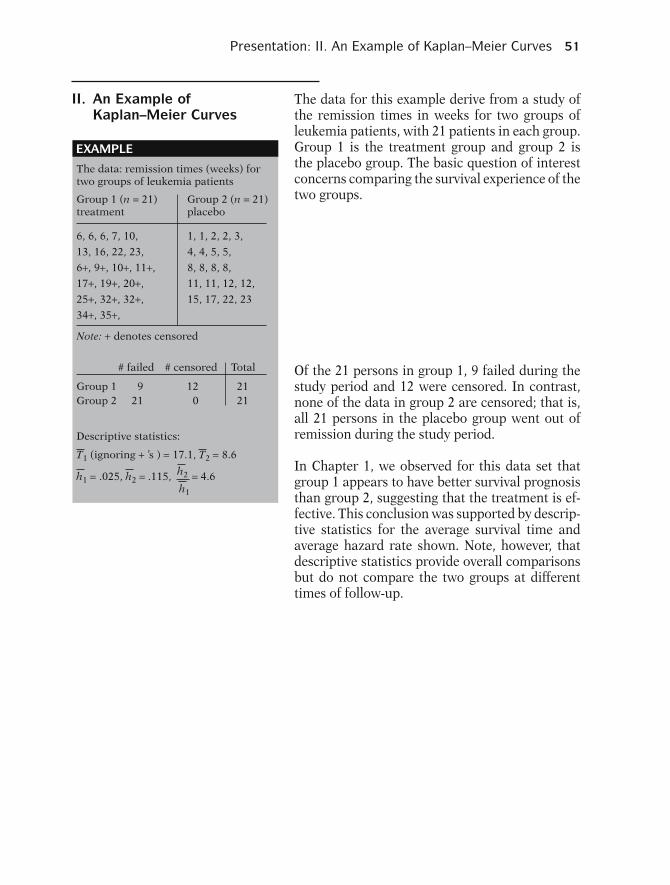
Presentation: II. An Example of Kaplan–Meier Curves 51
II. An Example ofKaplan–Meier Curves
The data for this example derive from a study ofthe remission times in weeks for two groups ofleukemia patients, with 21 patients in each group.Group 1 is the treatment group and group 2 isthe placebo group. The basic question of interestconcerns comparing the survival experience of thetwo groups.
EXAMPLE
The data: remission times (weeks) fortwo groups of leukemia patients
Group 1 (n = 21)treatment
Group 2 (n = 21)placebo
6, 6, 6, 7, 10,
13, 16, 22, 23,
6+, 9+, 10+, 11+,
17+, 19+, 20+,
25+, 32+, 32+,
34+, 35+,
1, 1, 2, 2, 3,
4, 4, 5, 5,
8, 8, 8, 8,
11, 11, 12, 12,
15, 17, 22, 23
Note: + denotes censored
Group 1Group 2
921
120
2121
# failed # censored Total
Descriptive statistics:
T1 (ignoring + ’s ) = 17.1, T2 = 8.6
h1 = .025, h2 = .115, h2 = 4.6h1
Of the 21 persons in group 1, 9 failed during thestudy period and 12 were censored. In contrast,none of the data in group 2 are censored; that is,all 21 persons in the placebo group went out ofremission during the study period.
In Chapter 1, we observed for this data set thatgroup 1 appears to have better survival prognosisthan group 2, suggesting that the treatment is ef-fective. This conclusion was supported by descrip-tive statistics for the average survival time andaverage hazard rate shown. Note, however, thatdescriptive statistics provide overall comparisonsbut do not compare the two groups at differenttimes of follow-up.

52 2. Kaplan–Meier Survival Curves and the Log–Rank Test
EXAMPLE (continued)
Ordered failure times:
Group 1 (treatment)
067
1013162223
>23
212117151211
76
—
03111111—
01120305—
t(j) nj mj qj
t(j) nj mj qj
Group 2 (placebo)
0123458
111215172223
21211917161412
864321
0221224221111
0000000000000
Group 2: no censored subjects
Group 2 (placebo)t( j)
0123458
111215172223
nj
21211917161412864321
mj
0221224221111
qj
0000000000000
S(t( j))
119/21 = .9017/21 = .8116/21 = .7614/21 = .6712/21 = .578/21 = .386/21 = .294/21 = .193/21 = .142/21 = .101/21 = .050/21 = .00
A table of ordered failure times is shown here foreach group. These tables provide the basic infor-mation for the computation of KM curves.
Each table begins with a survival time of zero, eventhough no subject actually failed at the start offollow-up. The reason for the zero is to allow forthe possibility that some subjects might have beencensored before the earliest failure time.
Also, each table contains a column denoted as n jthat gives the number of subjects in the risk set atthe start of the interval. Given that the risk set isdefined as the collection of individuals who havesurvived at least to time t( j ), it is assumed that n jincludes those persons failing at time t( j ). In otherwords, n j counts those subjects at risk for failinginstantaneously prior to time t( j ).
We now describe how to compute the KM curvefor the table for group 2. The computations forgroup 2 are quite straightforward because thereare no censored subjects for this group.
The table of ordered failure times for group 2is presented here again with the addition of an-other column that contains survival probabilityestimates. These estimates are the KM survivalprobabilities for this group. We will discuss thecomputations of these probabilities shortly.

Presentation: II. An Example of Kaplan–Meier Curves 53
KM Curve for Group 2 (Placebo)
S(t) = Pr (T > t)
0
.5
1
5 10 15 20
S(t)
Weeks
EXAMPLE (continued)
t(j) nj mj qj
Group 2 (placebo)
0123458
111215172223
21211917161412864321
0221224221111
0000000000000
119/21 = .9017/21 = .8116/21 = .7614/21 = .6712/21 = .57 8/21 = .38 6/21 = .29 4/21 = .19 3/21 = .14 2/21 = .10 1/21 = .05 0/21 = .00
S(t( j))
S(t( j))# surviving past t( j)
21=
No censorship in group 2
Alternative formula: KM approach
A plot of the KM survival probabilities correspond-ing to each ordered failure time is shown here forgroup 2. Empirical plots such as this one are typ-ically plotted as a step function that starts with ahorizontal line at a survival probability of 1 andthen steps down to the other survival probabili-ties as we move from one ordered failure time toanother.
We now describe how the survival probabilities forthe group 2 data are computed. Recall that a sur-vival probability gives the probability that a studysubject survives past a specified time.
Thus, considering the group 2 data, the probabil-ity of surviving past zero is unity, as it will alwaysbe for any data set.
Next, the probability of surviving past the first or-dered failure time of one week is given by 19/21 or(.90) because 2 people failed at one week, so that19 people from the original 21 remain as survivorspast one week.
Similarly, the next probability concerns subjectssurviving past two weeks, which is 17/21 (or .81)because 2 subjects failed at one week and 2 sub-jects failed at two weeks leaving 17 out of the orig-inal 21 subjects surviving past two weeks.
The remaining survival probabilities in the tableare computed in the same manner, that is, wecount the number of subjects surviving past thespecified time being considered and divide thisnumber by 21, the number of subjects at the startof follow-up.
Recall that no subject in group 2 was censored, sothe q column for group 2 consists entirely of ze-ros. If some of the q’s had been nonzero, an alter-native formula for computing survival probabili-ties would be needed. This alternative formula iscalled the Kaplan–Meier (KM) approach and canbe illustrated using the group 2 data even thoughall values of q are zero.

54 2. Kaplan–Meier Survival Curves and the Log–Rank Test
119 1721 19
1617
1416
1421
×× × × ==
=
=
=
1921
1617
17 = # in risk set at week 3
.67
Pr(T >1|T ≥ 1)
Pr(T >3|T ≥ 3)
S(4)
119 1721 19
1617
14 12 816 14 12
×× × × × ×=
119 1721 19
1617
1416
×× × ×=S(4)
S(8)
EXAMPLE
S(4) = = = .671 1921 19 17 16 21
17 16 14 14× × × ×
Pr(T > t( j) | T ≥ t( j))
KM formula = product limitformula
Group 1 (treatment)
t(j) nj mj qj S(t(j))
0 21 0 0 ©16 21 3 1 1 × 18
21···
For example, an alternative way to calculate thesurvival probability of exceeding four weeks forthe group 2 data can be written using the KM for-mula shown here. This formula involves the prod-uct of conditional probability terms. That is, eachterm in the product is the probability of exceed-ing a specific ordered failure time t( j ) given that asubject survives up to that failure time.
Thus, in the KM formula for survival past fourweeks, the term 19/21 gives the probability of sur-viving past the first ordered failure time, one week,given survival up to the first week. Note that all 21persons in group 2 survived up to one week, butthat 2 failed at one week, leaving 19 persons sur-viving past one week.
Similarly, the term 16/17 gives the probability ofsurviving past the third ordered failure time atweek 3, given survival up to week 3. There were17 persons who survived up to week 3 and one ofthese then failed, leaving 16 survivors past week 3.Note that the 17 persons in the denominator rep-resents the number in the risk set at week 3.
Notice that the product terms in the KM formulafor surviving past four weeks stop at the fourthweek with the component 14/16. Similarly, the KMformula for surviving past eight weeks stops at theeighth week.
More generally, any KM formula for a survivalprobability is limited to product terms up to thesurvival week being specified. That is why the KMformula is often referred to as a “product-limit”formula.
Next, we consider the KM formula for the datafrom group 1, where there are several censoredobservations.
The estimated survival probabilities obtained us-ing the KM formula are shown here for group 1.
The first survival estimate on the list is S(0) = 1, asit will always be, because this gives the probabilityof surviving past time zero.

Presentation: II. An Example of Kaplan–Meier Curves 55
Fraction at t( j): Pr(T > t( j) | T ≥ t( j))
Not available at t( j): failed prior to t( j)orcensored prior to t( j)
group 1 only
EXAMPLE (continued)
KM Plots for Remission Data
0
0.2
0
0.4
0.6
0.8
1
8 16 24 32
Group 2 (placebo)
Group 1 (treatment)
Group 1 (treatment)
0
6
7
10
13
16
22
23
21
21
17
15
12
11
7
6
0
3
1
1
1
1
1
1
0
1
1
2
0
3
0
5
1
118
1621
17
1514
1211
1110
76
65
.8571 ×
×
.8067
.8067 ×
.7529 ×
.7529
.6902 ×
.6902
.6275 ×
.6275
.5378 ×
.5378
.4482
.8571
t(j) nj mj qj S(t( j))
=
=
=
=
=
=
=
Obtain KM plots fromcomputer package, e.g., SAS,
Stata,SPSS
The other survival estimates are calculated by mul-tiplying the estimate for the immediately preced-ing failure time by a fraction. For example, thefraction is 18/21 for surviving past week 6, because21 subjects remain up to week 6 and 3 of thesesubjects fail to survive past week 6. The fraction is16/17 for surviving past week 7, because 17 peo-ple remain up to week 7 and one of these fails tosurvive past week 7. The other fractions are calcu-lated similarly.
For a specified failure time t( j ), the fraction may begenerally expressed as the conditional probabilityof surviving past time t( j ), given availability (i.e.,in the risk set) at time t( j ). This is exactly the sameformula that we previously used to calculate eachproduct term in the product limit formula used forthe group 2 data.
Note that a subject might not be available at timet( j ) for one of two reasons: (1) either the subjecthas failed prior to t( j ), or (2) the subject has beencensored prior to t( j ). Group 1 has censored ob-servations, whereas group 2 does not. Thus, forgroup 1, censored observations have to be takeninto account when determining the number avail-able at t( j ).
Plots of the KM curves for groups 1 and 2 areshown here on the same graph. Notice that theKM curve for group 1 is consistently higher thanthe KM curve for group 2. These figures indi-cate that group 1, which is the treatment group,has better survival prognosis than group 2, theplacebo group. Moreover, as the number of weeksincreases, the two curves appear to get fartherapart, suggesting that the beneficial effects of thetreatment over the placebo are greater the longerone stays in remission.
The KM plots shown above can be easily obtainedfrom most computer packages that perform sur-vival analysis, including SAS, Stata, and SPSS. Allthe user needs to do is provide a KM computerprogram with the basic data layout and then pro-vide appropriate commands to obtain plots.
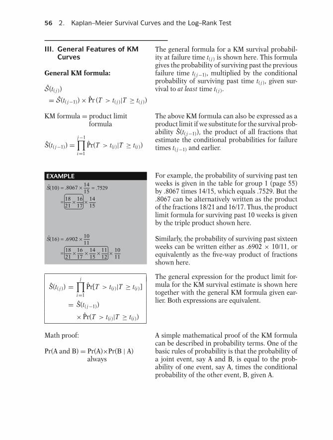
56 2. Kaplan–Meier Survival Curves and the Log–Rank Test
III. General Features of KMCurves
The general formula for a KM survival probabil-ity at failure time t( j ) is shown here. This formulagives the probability of surviving past the previousfailure time t( j−1), multiplied by the conditionalprobability of surviving past time t( j ), given sur-vival to at least time t( j ).
General KM formula:
S(t( j ))
= S(t( j−1)) × Pr (T > t( j )|T ≥ t( j ))
KM formula = product limitformula
S(t( j−1)) =j−1∏i=1
Pr(T > t(i)|T ≥ t(i))
The above KM formula can also be expressed as aproduct limit if we substitute for the survival prob-ability S(t( j−1)), the product of all fractions thatestimate the conditional probabilities for failuretimes t( j−1) and earlier.
EXAMPLE 1415
.8067 ×
1821 17 15
16 14× ×
S(10) =
=
1821 17 15 12 11
16 14 11 10× × × ×
1011
.6902 ×S(16) =
=
= .7529
For example, the probability of surviving past tenweeks is given in the table for group 1 (page 55)by .8067 times 14/15, which equals .7529. But the.8067 can be alternatively written as the productof the fractions 18/21 and 16/17. Thus, the productlimit formula for surviving past 10 weeks is givenby the triple product shown here.
Similarly, the probability of surviving past sixteenweeks can be written either as .6902 × 10/11, orequivalently as the five-way product of fractionsshown here.
S(t( j )) =j∏
i=1
Pr[T > t(i)|T ≥ t(i)]
= S(t( j−1))
× Pr(T > t(i)|T ≥ t(i))
The general expression for the product limit for-mula for the KM survival estimate is shown heretogether with the general KM formula given ear-lier. Both expressions are equivalent.
Math proof:
Pr(A and B) = Pr(A)×Pr(B | A)always
A simple mathematical proof of the KM formulacan be described in probability terms. One of thebasic rules of probability is that the probability ofa joint event, say A and B, is equal to the prob-ability of one event, say A, times the conditionalprobability of the other event, B, given A.

Presentation: IV. The Log–Rank Test for Two Groups 57
A = “T ≥ t( j )” → A and B = BB = “T > t( j )”
Pr(A and B) = Pr(B) = .....................................................................................................................................
......................................................................S(t( j ))
If we let A be the event that a subject survives toat least time t( j ) and we let B be the event that asubject survives past time t( j ), then the joint eventA and B simplifies to the event B, which is inclusiveof A. It follows that the probability of A and Bequals the probability of surviving past time t( j ).
No failures during t( j−1) < T < t( j )
Pr(A) = Pr(T > t( j−1)) = ........................................................................................................................................................
............................................................................................S(t( j−1))
Also, because t( j ) is the next failure time after t( j−1),there can be no failures after time t( j−1) and be-fore time t( j ). Therefore, the probability of A isequivalent to the probability of surviving past the( j − 1)th ordered failure time.
Pr(B|A) =....................................................................................................................................................................................................................................................................................
.........................................
.............................
.................................................
......................................................................................................................
Pr(T > t( j )|T ≥ t( j ))Furthermore, the conditional probability of Bgiven A is equivalent to the conditional probabilityin the KM formula.
Thus, from Pr(A and B) formula,
Pr(A and B) = Pr(A) × Pr(B | A)S(t( j )) = S(t( j−1))
× Pr(T > t( j )|T ≥ t( j ))
Thus, using the basic rules of probability, the KMformula can be derived.
IV. The Log–Rank Test forTwo Groups
We now describe how to evaluate whether or notKM curves for two or more groups are statisticallyequivalent. In this section we consider two groupsonly. The most popular testing method is calledthe log–rank test.
When we state that two KM curves are “statisti-cally equivalent,” we mean that, based on a testingprocedure that compares the two curves in some“overall sense,” we do not have evidence to indi-cate that the true (population) survival curves aredifferent.
Are KM curves statisticallyequivalent?
1.0
.8
.6
.4
.2
.08 16 24

58 2. Kaplan–Meier Survival Curves and the Log–Rank Test
� Chi-square test� Overall comparison of KMcurves� Observed versus expectedcounts� Categories defined by orderedfailure times
The log–rank test is a large-sample chi-square testthat uses as its test criterion a statistic that pro-vides an overall comparison of the KM curves be-ing compared. This (log–rank) statistic, like manyother statistics used in other kinds of chi-squaretests, makes use of observed versus expected cellcounts over categories of outcomes. The cate-gories for the log–rank statistic are defined by eachof the ordered failure times for the entire set ofdata being analyzed.
EXAMPLE
1
2
3
4
5
6
7
8
10
11
12
13
15
16
17
22
23
0
0
0
0
0
3
1
0
1
0
0
1
0
1
0
1
1
2
2
1
2
2
0
0
4
0
2
2
0
1
0
1
1
1
21
21
21
21
21
21
17
16
15
13
12
12
11
11
10
7
6
21
19
17
16
14
12
12
12
8
8
6
4
4
3
3
2
1
Remission data: n = 42
# failures # in risk sett(j) m1j m2j n1j n2j
As an example of the information required for thelog–rank test, we again consider the comparisonof the treatment (group 1) and placebo (group 2)subjects in the remission data on 42 leukemia pa-tients.
Here, for each ordered failure time, t( j ), in the en-tire set of data, we show the numbers of subjects(mi j ) failing at that time, separately by group (i),followed by the numbers of subjects (ni j ) in therisk set at that time, also separately by group.
Thus, for example, at week 4, no subjects failed ingroup 1, whereas two subjects failed in group 2.Also, at week 4, the risk set for group 1 contains21 persons, whereas the risk set for group 2 con-tains 16 persons.
Similarly, at week 10, one subject failed in group 1,and no subjects failed at group 2; the risk sets foreach group contain 15 and 8 subjects, respectively.
Expected cell counts:
e1 j =(
n1 j
n1 j + n2 j
)× (m1 j + m2 j )
↑ ↑Proportion # of failures over
in risk set both groups
e2 j =(
n2 j
n1 j + n2 j
)× (m1 j + m2 j )
We now expand the previous table to include ex-pected cell counts and observed minus expectedvalues for each group at each ordered failuretime. The formula for the expected cell countsis shown here for each group. For group 1, thisformula computes the expected number at time j(i.e., e1 j ) as the proportion of the total subjectsin both groups who are at risk at time j, thatis, n1 j /(n1 j + n2 j ), multiplied by the total num-ber of failures at that time for both groups (i.e.,m1 j + m2 j ). For group 2, e2 j is computed simi-larly.

Presentation: IV. The Log–Rank Test for Two Groups 59
EXAMPLE
Expanded Table (Remission Data)
# failures # in risk set # expected Observed–expected
j t( j) m1j m2j n1j n2j e1j e2j m1j – e1j m2j – e2j
1
2
3
4
5
6
7
8
9
10
11
12
13
14
15
16
17
1
2
3
4
5
6
7
8
10
11
12
13
15
16
17
22
23
0
0
0
0
0
3
1
0
1
0
0
1
0
1
0
1
1
2
2
1
2
2
0
0
4
0
2
2
0
1
0
1
1
1
21
21
21
21
21
21
17
16
15
13
12
12
11
11
10
7
6
21
19
17
16
14
12
12
12
8
8
6
4
4
3
3
2
1
(21/42) × 2
(21/40) × 2
(21/38) × 1
(21/37) × 2
(21/35) × 2
(21/33) × 3
(17/29) × 1
(16/28) × 4
(15/23) × 1
(13/21) × 2
(12/18) × 2
(12/16) × 1
(11/15) × 1
(11/14) × 1
(10/13) × 1
(7/9) × 2
(6/7) × 2
(21/42) × 2
(19/40) × 2
(17/38) × 1
(16/37) × 2
(14/35) × 2
(12/33) × 3
(12/29) × 1
(12/28) × 4
(8/23) × 1
(8/21) × 2
(6/18) × 2
(4/16) × 1
(4/15) × 1
(3/14) × 1
(3/13) × 1
(2/9) × 2
(1/7) × 2
−1.00
−1.05
−0.55
−1.14
−1.20
1.09
0.41
−2.29
0.35
−1.24
−1.33
0.25
−0.73
0.21
−0.77
−0.56
−0.71
1.00
1.05
0.55
1.14
1.20
−1.09
−0.41
2.29
−0.35
1.24
1.33
−0.25
0.73
−0.21
0.77
0.56
0.71
Totals 9 21 19.26 10.74 −10.26 −10.26
# of failure times↓
Oi − E j =17∑j=1
(mi j − ei j ),
i = 1, 2
O1 − E1 = −10.26
O2 − E2 = 10.26
EXAMPLE
When two groups are being compared, the log–rank test statistic is formed using the sum of theobserved minus expected counts over all failuretimes for one of the two groups. In this exam-ple, this sum is −10.26 for group 1 and 10.26 forgroup 2. We will use the group 2 value to carry outthe test, but as we can see, except for the minussign, the difference is the same for the two groups.
Two groups:O2 − E2 = summed observedminus expected score for group 2
Log–rank statistic = (O2 − E2)2
Var(O2 − E2)
For the two-group case, the log–rank statistic,shown here at the left, is computed by dividing thesquare of the summed observed minus expectedscore for one of the groups—say, group 2—by thevariance of the summed observed minus expectedscore.

60 2. Kaplan–Meier Survival Curves and the Log–Rank Test
Var(Oi − Ei )
=∑
j
n1 j n2 j (m1 j + m2 j )(n1 j + n2 j − m1 j − m2 j )(n1 j + n2 j )2(n1 j + n2 j − 1)
i = 1, 2
The expression for the estimated variance isshown here. For two groups, the variance formulais the same for each group. This variance formulainvolves the number in the risk set in each group(ni j ) and the number of failures in each group(mi j ) at time j. The summation is over all distinctfailure times.
H0: no difference between survivalcurves
Log–rank statistic ∼χ2 with 1 dfunder H0
The null hypothesis being tested is that there is nooverall difference between the two survival curves.Under this null hypothesis, the log–rank statisticis approximately chi-square with one degree offreedom. Thus, a P-value for the log–rank test isdetermined from tables of the chi-square distri-bution.
Computer programs:Stata’s “sts test”:
� descriptive statistics for KMcurves� log–rank statistic� Alternative statistics to log–rankstatistic
Several computer programs are available forcalculating the log–rank statistic. For examplethe Stata package has a command called “ststest” that computes descriptive information aboutKaplan–Meier curves, the log–rank statistic, andalternative statistics to the log–rank statistic, tobe described later. Other packages, like SAS andSPSS, have procedures that provide results sim-ilar to those of Stata. A comparison of Stata,SAS, and SPSS procedures and output is pro-vided in the Computer Appendix at the back of thistext.
EXAMPLE Using Stata: Remission Data
GroupEvents
observedEvents
expected
921
12
30 30.00
19.2510.75
Total
Log-rank = chi2(2) = 16.79P-value = Pr > chi2 = 0.000
For the remission data, the edited printout fromusing the Stata “sts test” procedure is shown here.The log–rank statistic is 16.79 and the correspond-ing P-value is zero to three decimal places. ThisP-value indicates that the null hypothesis shouldbe rejected. We can therefore conclude that thetreatment and placebo groups have significantlydifferent KM survival curves.
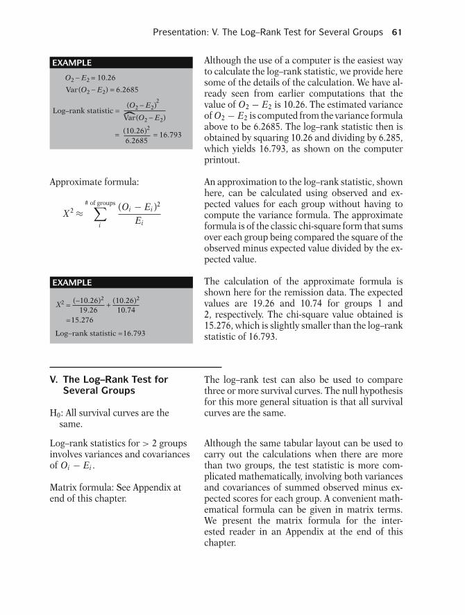
Presentation: V. The Log–Rank Test for Several Groups 61
EXAMPLE
O2 − E2 = 10.26
Var(O2 − E2) = 6.2685
Log–rank statistic =(O2 − E2)
Var(O2 − E2)
2
2(10.26)6.2685
= = 16.793
ˆ
Although the use of a computer is the easiest wayto calculate the log–rank statistic, we provide heresome of the details of the calculation. We have al-ready seen from earlier computations that thevalue of O2 − E2 is 10.26. The estimated varianceof O2 − E2 is computed from the variance formulaabove to be 6.2685. The log–rank statistic then isobtained by squaring 10.26 and dividing by 6.285,which yields 16.793, as shown on the computerprintout.
Approximate formula:
X 2 ≈# of groups∑
i
(Oi − Ei )2
Ei
An approximation to the log–rank statistic, shownhere, can be calculated using observed and ex-pected values for each group without having tocompute the variance formula. The approximateformula is of the classic chi-square form that sumsover each group being compared the square of theobserved minus expected value divided by the ex-pected value.
EXAMPLE
Log−rank statistic =16.793
=15.276
=X2
19.26(−10.26)2
10.74(10.26)2
+
The calculation of the approximate formula isshown here for the remission data. The expectedvalues are 19.26 and 10.74 for groups 1 and2, respectively. The chi-square value obtained is15.276, which is slightly smaller than the log–rankstatistic of 16.793.
V. The Log–Rank Test forSeveral Groups
The log–rank test can also be used to comparethree or more survival curves. The null hypothesisfor this more general situation is that all survivalcurves are the same.H0: All survival curves are the
same.
Log–rank statistics for > 2 groupsinvolves variances and covariancesof Oi − Ei .
Matrix formula: See Appendix atend of this chapter.
Although the same tabular layout can be used tocarry out the calculations when there are morethan two groups, the test statistic is more com-plicated mathematically, involving both variancesand covariances of summed observed minus ex-pected scores for each group. A convenient math-ematical formula can be given in matrix terms.We present the matrix formula for the inter-ested reader in an Appendix at the end of thischapter.
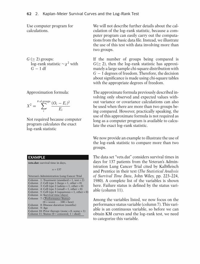
62 2. Kaplan–Meier Survival Curves and the Log–Rank Test
Use computer program forcalculations.
We will not describe further details about the cal-culation of the log–rank statistic, because a com-puter program can easily carry out the computa-tions from the basic data file. Instead, we illustratethe use of this test with data involving more thantwo groups.
G (≥ 2) groups:log–rank statistic ∼χ2 withG − 1 df
If the number of groups being compared isG(≥ 2), then the log–rank statistic has approxi-mately a large sample chi-square distribution withG − 1 degrees of freedom. Therefore, the decisionabout significance is made using chi-square tableswith the appropriate degrees of freedom.
Approximation formula:
X 2 =# of groups∑
i
(Oi − Ei )2
Ei
Not required because computerprogram calculates the exactlog–rank statistic
The approximate formula previously described in-volving only observed and expected values with-out variance or covariance calculations can alsobe used when there are more than two groups be-ing compared. However, practically speaking, theuse of this approximate formula is not required aslong as a computer program is available to calcu-late the exact log–rank statistic.
We now provide an example to illustrate the use ofthe log–rank statistic to compare more than twogroups.
EXAMPLE vets.dat: survival time in days,
Column 1: Treatment (standard = 1, test = 2)Column 2: Cell type 1 (large = 1, other = 0)Column 3: Cell type 2 (adeno = 1, other = 0)Column 4: Cell type 3 (small = 1, other = 0)Column 5: Cell type 4 (squamous = 1, other = 0)Column 6: Survival time (days)
Column 8: Disease duration (months)Column 9: AgeColumn 10: Prior therapy (none = 0, some = 1)Column 11: Status (0 = censored, 1 = died)
Column 7: Performance Status(0 = worst . . . 100 = best)
n = 137
Veteran’s Administration Lung Cancer Trial
The data set “vets.dat” considers survival times indays for 137 patients from the Veteran’s Admin-istration Lung Cancer Trial cited by Kalbfleischand Prentice in their text (The Statistical Analysisof Survival Time Data, John Wiley, pp. 223–224,1980). A complete list of the variables is shownhere. Failure status is defined by the status vari-able (column 11).
Among the variables listed, we now focus on theperformance status variable (column 7). This vari-able is an continuous variable, so before we canobtain KM curves and the log–rank test, we needto categorize this variable.

Presentation: VI. Alternatives to the Log Rank Test 63
Performance Status Categories
Group #
123
Categories Size
525035
KM curves for performance status groups
Eventsobserved
EventsexpectedGroup
123
504731
26.3055.1746.53
TotalLog–rank = chi2(2) = 29.18P-value = Pr > chi2 = 0.0000G = 3 groups; df = G – 1 = 2
128 128.00
Log–rank test is highly significant.
Conclude significant difference amongthree survival curves.
EXAMPLE (continued)
1.0
0.5
0.0
0 100 200 300 400 500 600
1
1
111
1
2222
2 33
33
22
60–7475–100
0–59
If, for the performance status variable, we choosethe categories 0–59, 60–74, and 75–100, we obtainthree groups of sizes 52, 50, and 35, respectively.
The KM curves for each of three groups are shownhere. Notice that these curves appear to be quitedifferent. A test of significance of this difference isprovided by the log–rank statistic.
An edited printout of descriptive informationabout the three KM curves together with the log–rank test results are shown here. These resultswere obtained using the Stata package.
Because three groups are being compared here,G = 3 and the degrees of freedom for the log–rank test is thus G − 1, or 2. The log–rank statisticis computed to be 29.181, which has a P-value ofzero to three decimal places. Thus, the conclusionfrom the log–rank test is that there is a highly sig-nificant difference among the three survival curvesfor the performance status groups.
VI. Alternatives to the LogRank Test
There are several alternatives to the log rank testoffered by Stata, SAS, and SPSS designed to testthe hypothesis that two or more survival curvesare equivalent. In this section we describe theWilcoxon, the Tarone–Ware, the Peto, and theFlemington–Harrington test. All of these testsare variations of the log rank test and are easilyimplemented in Stata.
Alternative tests supported by Stata
WilcoxenTarone–WarePetoFlemington–Harrington
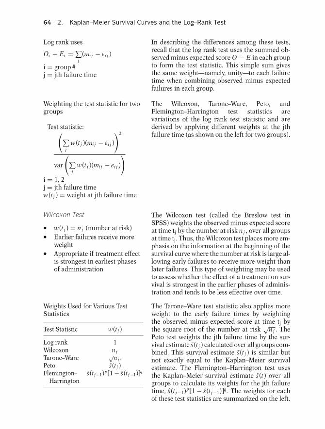
64 2. Kaplan–Meier Survival Curves and the Log–Rank Test
Log rank uses
Oi − Ei = ∑j
(mi j − ei j )
i = group #j = jth failure time
In describing the differences among these tests,recall that the log rank test uses the summed ob-served minus expected score O − E in each groupto form the test statistic. This simple sum givesthe same weight—namely, unity—to each failuretime when combining observed minus expectedfailures in each group.
Weighting the test statistic for twogroups
Test statistic:(∑j
w(t j )(mi j − ei j )
)2
var
(∑j
w(t j )(mi j − ei j )
)i = 1, 2j = jth failure timew(t j ) = weight at jth failure time
The Wilcoxon, Tarone–Ware, Peto, andFlemington–Harrington test statistics arevariations of the log rank test statistic and arederived by applying different weights at the jthfailure time (as shown on the left for two groups).
Wilcoxon Test
� w(t j ) = n j (number at risk)� Earlier failures receive moreweight� Appropriate if treatment effectis strongest in earliest phasesof administration
The Wilcoxon test (called the Breslow test inSPSS) weights the observed minus expected scoreat time tj by the number at risk n j , over all groupsat time tj. Thus, the Wilcoxon test places more em-phasis on the information at the beginning of thesurvival curve where the number at risk is large al-lowing early failures to receive more weight thanlater failures. This type of weighting may be usedto assess whether the effect of a treatment on sur-vival is strongest in the earlier phases of adminis-tration and tends to be less effective over time.
Weights Used for Various TestStatistics
Test Statistic w(t j )
Log rank 1Wilcoxon n j
Tarone–Ware√
n j .
Peto s(t j )Flemington– s(t j−1)p[1 − s(t j−1)]q
Harrington
The Tarone–Ware test statistic also applies moreweight to the early failure times by weightingthe observed minus expected score at time tj bythe square root of the number at risk
√n j . The
Peto test weights the jth failure time by the sur-vival estimate s(t j ) calculated over all groups com-bined. This survival estimate s(t j ) is similar butnot exactly equal to the Kaplan–Meier survivalestimate. The Flemington–Harrington test usesthe Kaplan–Meier survival estimate s(t) over allgroups to calculate its weights for the jth failuretime, s(t j−1)p[1 − s(t j−1)]q . The weights for eachof these test statistics are summarized on the left.

Presentation: VI. Alternatives to the Log Rank Test 65
Flemington–Harrington Test
w(t) = s(t j−1)p[1 − s(t j−1)]q
if p = 1 and q = 0, w(t) = s(t j−1)if p = 0 and q = 1,
w(t) = 1 − s(t j−1)if p = 0 and q = 0,
w(t) = 1 (log rank test)
The Flemington–Harrington test allows the mostflexibility in terms of the choice of weights becausethe user provides the values of p and q. For exam-ple, if p = 1 and q = 0 then w(t) = s(t j−1) whichgives more weight for the earlier survival timeswhen s(t j−1) is close to one. However, if p = 0 andq = 1 then w(t) = 1 − s(t j−1) in which case thelater survival times receive more weight. If p = 0and q = 0 then w(t) = 1, and the Flemington–Harrington test reduces to the log rank test.
Comparisons of Test Results:Remission Data, TestingTreatment (RX)
Chi-squareTest (1 df) P-value
Log rank 16.79 0.0000Wilcoxon 13.46 0.0002Tarone– 15.12 0.0001
WarePeto 14.08 0.0002FH (p = 3, 8.99 0.0027
q = 1)FH (p = 1, 12.26 0.0005
q = 3)
On the left is a comparison of test results for theeffect of treatment (vs. placebo) using the remis-sion data. The log rank chi-square statistic (alsodisplayed previously in this chapter) is the high-est among these tests at 16.79. The Flemington–Harrington (FH) test with p = 3 and q = 1 yieldedthe lowest chi-square value at 8.99, although withthis weighting it is not immediately obvious whichpart of the survival curve is getting the mostweight. However, all the test results are highly sig-nificant yielding a similar conclusion to reject thenull hypothesis.
Vets Data, 3-Level PerformanceStatus
Chi-squareTest (2 df) P-value
Log rank 29.18 0.0000Wilcoxon 46.10 0.0000
Remission Data, 2-Level Treatment
Chi-squareTest (1 df) P-value
Log rank 16.79 0.0000Wilcoxon 13.46 0.0002
On the left are comparisons of the log rank andWilcoxon tests for the 3-level performance statusvariable from the vets dataset discussed in the pre-vious section. The Wilcoxon test yields a higherchi-square value (46.10) than the log rank test(29.18). In contrast, the log rank test for the ef-fect of treatment (RX) from the remissions datayields a higher chi-square value (16.79) than theWilcoxon test (13.46). However, both the Wilcoxonand log rank tests are highly significant for bothperformance status and for treatment.
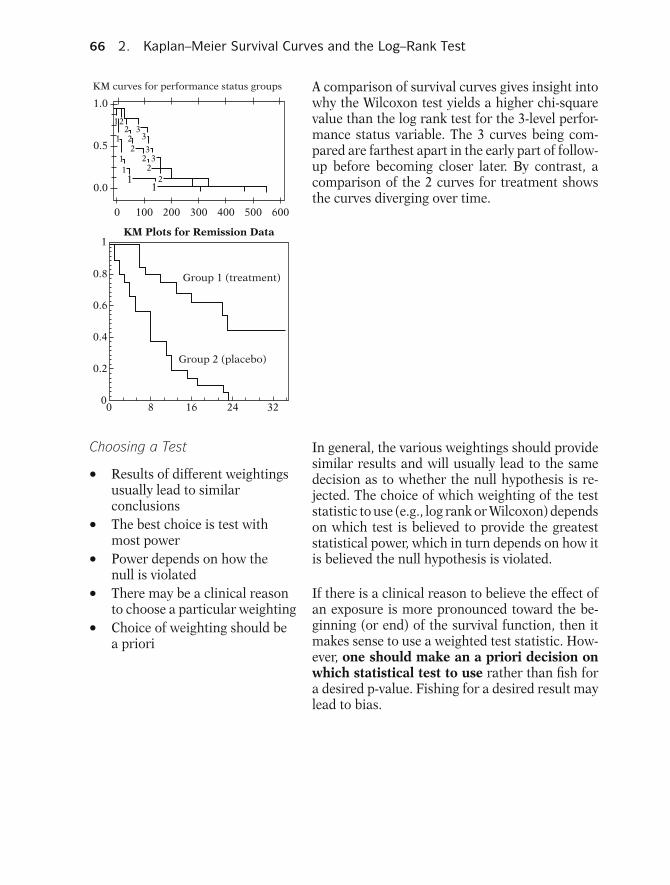
66 2. Kaplan–Meier Survival Curves and the Log–Rank Test
KM curves for performance status groups
1.0
0.5
0.0
0 100 200 300 400 500 600
1
1
111
1
2222
2 33
33
22
KM Plots for Remission Data
0
0.2
0
0.4
0.6
0.8
1
8 16 24 32
Group 2 (placebo)
Group 1 (treatment)
A comparison of survival curves gives insight intowhy the Wilcoxon test yields a higher chi-squarevalue than the log rank test for the 3-level perfor-mance status variable. The 3 curves being com-pared are farthest apart in the early part of follow-up before becoming closer later. By contrast, acomparison of the 2 curves for treatment showsthe curves diverging over time.
Choosing a Test
� Results of different weightingsusually lead to similarconclusions� The best choice is test withmost power� Power depends on how thenull is violated
In general, the various weightings should providesimilar results and will usually lead to the samedecision as to whether the null hypothesis is re-jected. The choice of which weighting of the teststatistic to use (e.g., log rank or Wilcoxon) dependson which test is believed to provide the greateststatistical power, which in turn depends on how itis believed the null hypothesis is violated.
� There may be a clinical reasonto choose a particular weighting� Choice of weighting should bea priori
If there is a clinical reason to believe the effect ofan exposure is more pronounced toward the be-ginning (or end) of the survival function, then itmakes sense to use a weighted test statistic. How-ever, one should make an a priori decision onwhich statistical test to use rather than fish fora desired p-value. Fishing for a desired result maylead to bias.
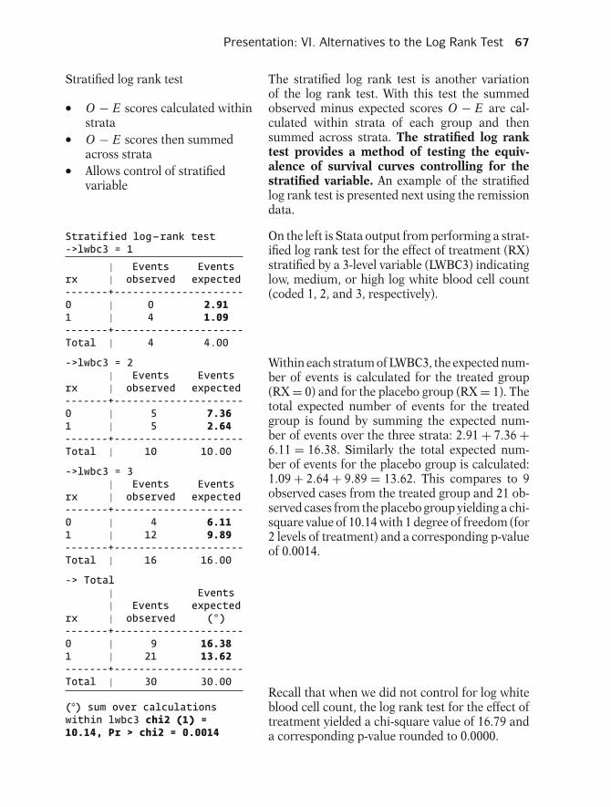
Presentation: VI. Alternatives to the Log Rank Test 67
Stratified log rank test
� O − E scores calculated withinstrata� O − E scores then summedacross strata� Allows control of stratifiedvariable
The stratified log rank test is another variationof the log rank test. With this test the summedobserved minus expected scores O − E are cal-culated within strata of each group and thensummed across strata. The stratified log ranktest provides a method of testing the equiv-alence of survival curves controlling for thestratified variable. An example of the stratifiedlog rank test is presented next using the remissiondata.
Stratified log--rank test->lwbc3 = 1
| Events Eventsrx | observed expected-------+---------------------0 | 0 2.911 | 4 1.09-------+---------------------Total | 4 4.00
->lwbc3 = 2| Events Events
rx | observed expected-------+---------------------0 | 5 7.361 | 5 2.64-------+---------------------Total | 10 10.00
->lwbc3 = 3| Events Events
rx | observed expected-------+---------------------0 | 4 6.111 | 12 9.89-------+---------------------Total | 16 16.00
-> Total| Events| Events expected
rx | observed (*)-------+---------------------0 | 9 16.381 | 21 13.62-------+---------------------Total | 30 30.00
(*) sum over calculationswithin lwbc3 chi2 (1) =10.14, Pr > chi2 = 0.0014
On the left is Stata output from performing a strat-ified log rank test for the effect of treatment (RX)stratified by a 3-level variable (LWBC3) indicatinglow, medium, or high log white blood cell count(coded 1, 2, and 3, respectively).
Within each stratum of LWBC3, the expected num-ber of events is calculated for the treated group(RX = 0) and for the placebo group (RX = 1). Thetotal expected number of events for the treatedgroup is found by summing the expected num-ber of events over the three strata: 2.91 + 7.36 +6.11 = 16.38. Similarly the total expected num-ber of events for the placebo group is calculated:1.09 + 2.64 + 9.89 = 13.62. This compares to 9observed cases from the treated group and 21 ob-served cases from the placebo group yielding a chi-square value of 10.14 with 1 degree of freedom (for2 levels of treatment) and a corresponding p-valueof 0.0014.
Recall that when we did not control for log whiteblood cell count, the log rank test for the effect oftreatment yielded a chi-square value of 16.79 anda corresponding p-value rounded to 0.0000.
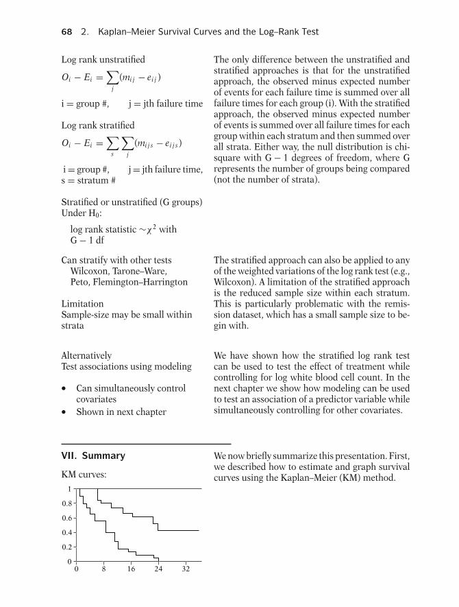
68 2. Kaplan–Meier Survival Curves and the Log–Rank Test
Log rank unstratified
Oi − Ei =∑
j
(mi j − ei j )
i = group #, j = jth failure time
Log rank stratified
Oi − Ei =∑
s
∑j
(mi j s − ei j s)
i = group #, j = jth failure time,s = stratum #
Stratified or unstratified (G groups)Under H0:
log rank statistic ∼χ2 withG − 1 df
The only difference between the unstratified andstratified approaches is that for the unstratifiedapproach, the observed minus expected numberof events for each failure time is summed over allfailure times for each group (i). With the stratifiedapproach, the observed minus expected numberof events is summed over all failure times for eachgroup within each stratum and then summed overall strata. Either way, the null distribution is chi-square with G − 1 degrees of freedom, where Grepresents the number of groups being compared(not the number of strata).
Can stratify with other testsWilcoxon, Tarone–Ware,Peto, Flemington–Harrington
LimitationSample-size may be small withinstrata
The stratified approach can also be applied to anyof the weighted variations of the log rank test (e.g.,Wilcoxon). A limitation of the stratified approachis the reduced sample size within each stratum.This is particularly problematic with the remis-sion dataset, which has a small sample size to be-gin with.
AlternativelyTest associations using modeling
� Can simultaneously controlcovariates� Shown in next chapter
We have shown how the stratified log rank testcan be used to test the effect of treatment whilecontrolling for log white blood cell count. In thenext chapter we show how modeling can be usedto test an association of a predictor variable whilesimultaneously controlling for other covariates.
VII. Summary We now briefly summarize this presentation. First,we described how to estimate and graph survivalcurves using the Kaplan–Meier (KM) method.KM curves:
1
0.8
0.6
0.4
0.2
00 8 16 24 32
Presentation: VII. Summary 69
t( j ) : j th ordered failure time
S(t( j )) =j∏
i=1
Pr[T > t(i)|T ≥ t(i)]
= S(t( j−1))
×Pr(T > t(i)|T ≥ t(i))
To compute KM curves, we must form a data lay-out that orders the failure times from smallest tolargest. For each ordered failure time, the esti-mated survival probability is computed using theproduct limit formula shown here. Alternatively,this estimate can be computed as the product ofthe survival estimate for the previous failure timemultiplied by the conditional probability of sur-viving past the current failure time.
Log–rank test:H0: common survival curve forall groups
Log–rank statistic = (O2 − E2)2
Var(O2 − E2)
log–rank statistic ∼χ2 with G − 1d f under H0
G = # of groups
When survival curves are being compared, the log–rank test gives a statistical test of the null hypoth-esis of a common survival curve. For two groups,the log–rank statistic is based on the summed ob-served minus expected scores for a given groupand its variance estimate. For several groups, acomputer should always be used since the log–rank formula is more complicated mathemati-cally. The test statistic is approximately chi-squarein large samples with G − 1 degrees of freedom,where G denotes the number of groups being com-pared.
Chapters This presentation is now complete. You can reviewthis presentation using the detailed outline thatfollows and then try the practice exercises and test.
1. Introduction✓ 2. Kaplan–Meier Survival Curves
and the Log–Rank Test
��
��
Next:
3. The Cox Proportional HazardsModel and Its Characteristics
Chapter 3 introduces the Cox proportional haz-ards (PH) model, which is the most popular math-ematical modeling approach for estimating sur-vival curves when considering several explanatoryvariables simultaneously.
70 2. Kaplan–Meier Survival Curves and the Log–Rank Test
DetailedOutline
I. Review (pages 48–50)A. The outcome variable is (survival) time until an
event (failure) occurs.B. Key problem: censored data, i.e., don’t know
survival time exactly.C. Notation: T = survival time random variable
t = specific value of Tδ = (0, 1) variable for failure/
censorship statusS(t) = survivor functionh(t) = hazard function
D. Properties of survivor function:i. theoretically, graph is smooth curve, decreasing
from S(t) = 1 at time t = 0 to S(t) = 0 att = ∞;
ii. in practice, graph is step function.E. Properties of h(t):
i. instantaneous potential for failing givensurvival up to time;
ii. h(t) is a rate; ranges from 0 to ∞.F. Relationship of S(t) to h(t): if you know one you
can determine the other.G. Goals of survival analysis: estimation of survivor
and hazard functions; comparisons andrelationships of explanatory variables to survival.
H. Data layoutsi. for the computer;
ii. for understanding the analysis: involves risksets.
II. An Example of Kaplan–Meier Curves (pages 51–55)A. Data are from study of remission times in weeks for
two groups of leukemia patients (21 in each group).B. Group 1 (treatment group) has several censored
observations, whereas group 2 has no censoredobservations.
C. Table of ordered failure times is provided for eachgroup.
D. For group 2 (all noncensored), survival probabilitiesare estimated directly and plotted. Formula used is
S(t( j )) = # surviving past t( j )
21.

Detailed Outline 71
E. Alternative approach for group 2 is given by aproduct limit formula.
F. For group 1, survival probabilities calculated bymultiplying estimate for immediately precedingfailure time by a conditional probability ofsurviving past current failure time, i.e.,
S( j ) = S( j−1) Pr[T > t( j )|T ≥ t( j )].
III. General Features of KM Curves (pages 56–57)A. Two alternative general formulae:
S( j ) =j∏
i=1
Pr[T > t(i)|T ≥ t(i)] (product limitformula)
S( j ) = S( j−1)Pr[T > t( j )|T ≥ t( j )]
B. Second formula derived from probability rule:
Pr(A and B) = Pr(A) × Pr(B|A)
IV. The Log–Rank Test for Two Groups (pages 57–61)A. Large sample chi-square test; provides overall
comparison of KM curves.B. Uses observed versus expected counts over
categories of outcomes, where categories aredefined by ordered failure times for entire set ofdata.
C. Example provided using remission data involvingtwo groups:i. expanded table described to show how
expected and observed minus expected cellcounts are computed.
ii. for ith group at time j, where i = 1 or 2:
observed counts = mi j ,expected counts = ei j , whereexpected counts = (proportion in risk set) ×(# failures over both groups),
i.e., ei j =(
ni j
n1 j + n2 j
)(m1 j + m2 j ).
D. Log–rank statistic for two groups:
(Oi − Ei )2
Var(Oi − Ei ),
where i = 1, 2,

72 2. Kaplan–Meier Survival Curves and the Log–Rank Test
Oi − Ei =∑
j
(mi j − ei j ), and
Var(Oi − Ei )
=∑
j
n1 j n2 j (m1 j + m2 j )(n1 j + n2 j − m1 j − m2 j )(n1 j + n2 j )2(n1 j + n2 j − 1)
,
i = 1, 2E. H0: no difference between survival curves.F. Log–rank statistic ∼χ2 with 1 df under H0.G. Approximate formula:
X 2 =G∑
i=1
(Oi − Ei )2
Ei, where G = 2 = # of groups
H. Remission data example: Log–rank statistic =16.793, whereas X 2 = 15.276.
V. The Log–Rank Test for Several Groups(pages 61–63)A. Involves variances and covariances; matrix
formula in Appendix.B. Use computer for calculations.C. Under H0, log–rank statistic ∼χ2 with G − 1 df,
where G = # of groups.D. Example provided using vets.dat with interval
variable “performance status”; this variable iscategorized into G = 3 groups, so df for log–ranktest is G − 1 = 2, log–rank statistic is 29.181(P = 0.0).
VI. Alternatives to the Log–rank Test (pages 63–68)A. Alternative tests supported by Stata:
Wilcoxen, Tarone-Ware, Peto, andFlemington-Harrington.
B. Alternative tests differ by applying differentweights at the j-th failure time.
C. The choice of alternative depends on the reasonfor the belief that the effect is more pronouncedtowards the beginning (or end) of the survivalfunction.
D. The stratified-log–rank test is a variation of thelog–rank test that controls for one or morestratified variables.
VII. Summary (page 68)
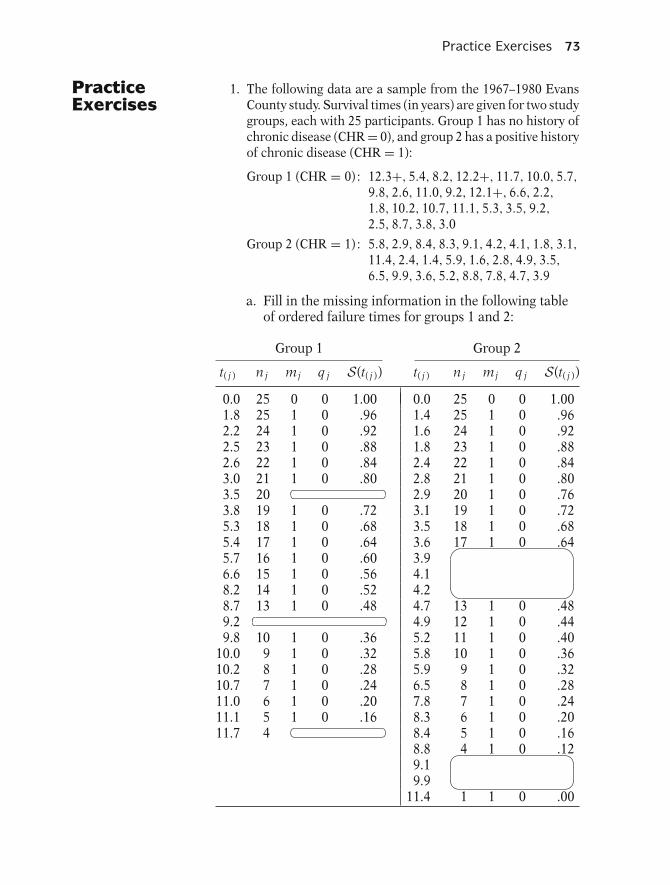
Practice Exercises 73
PracticeExercises
1. The following data are a sample from the 1967–1980 EvansCounty study. Survival times (in years) are given for two studygroups, each with 25 participants. Group 1 has no history ofchronic disease (CHR = 0), and group 2 has a positive historyof chronic disease (CHR = 1):
Group 1 (CHR = 0) : 12.3+, 5.4, 8.2, 12.2+, 11.7, 10.0, 5.7,
9.8, 2.6, 11.0, 9.2, 12.1+, 6.6, 2.2,
1.8, 10.2, 10.7, 11.1, 5.3, 3.5, 9.2,
2.5, 8.7, 3.8, 3.0
Group 2 (CHR = 1) : 5.8, 2.9, 8.4, 8.3, 9.1, 4.2, 4.1, 1.8, 3.1,
11.4, 2.4, 1.4, 5.9, 1.6, 2.8, 4.9, 3.5,
6.5, 9.9, 3.6, 5.2, 8.8, 7.8, 4.7, 3.9
a. Fill in the missing information in the following tableof ordered failure times for groups 1 and 2:
Group 1 Group 2
t( j ) n j mj q j S(t( j )) t( j ) n j mj q j S(t( j ))
0.0 25 0 0 1.00 0.0 25 0 0 1.001.8 25 1 0 .96 1.4 25 1 0 .962.2 24 1 0 .92 1.6 24 1 0 .922.5 23 1 0 .88 1.8 23 1 0 .882.6 22 1 0 .84 2.4 22 1 0 .843.0 21 1 0 .80 2.8 21 1 0 .803.5 20
�� � 2.9 20 1 0 .763.8 19 1 0 .72 3.1 19 1 0 .725.3 18 1 0 .68 3.5 18 1 0 .685.4 17 1 0 .64 3.6 17 1 0 .645.7 16 1 0 .60 3.9
�
�
6.6 15 1 0 .56 4.18.2 14 1 0 .52 4.28.7 13 1 0 .48 4.7 13 1 0 .489.2
�� � 4.9 12 1 0 .449.8 10 1 0 .36 5.2 11 1 0 .40
10.0 9 1 0 .32 5.8 10 1 0 .3610.2 8 1 0 .28 5.9 9 1 0 .3210.7 7 1 0 .24 6.5 8 1 0 .2811.0 6 1 0 .20 7.8 7 1 0 .2411.1 5 1 0 .16 8.3 6 1 0 .2011.7 4
�� � 8.4 5 1 0 .168.8 4 1 0 .129.1
��
��9.9
11.4 1 1 0 .00
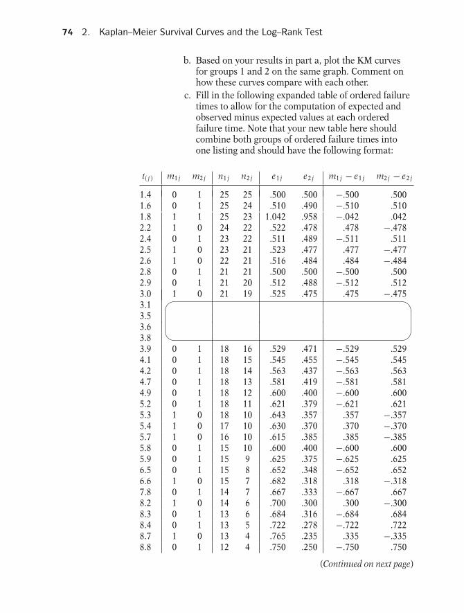
74 2. Kaplan–Meier Survival Curves and the Log–Rank Test
b. Based on your results in part a, plot the KM curvesfor groups 1 and 2 on the same graph. Comment onhow these curves compare with each other.
c. Fill in the following expanded table of ordered failuretimes to allow for the computation of expected andobserved minus expected values at each orderedfailure time. Note that your new table here shouldcombine both groups of ordered failure times intoone listing and should have the following format:
t( j ) m1 j m2 j n1 j n2 j e1 j e2 j m1 j − e1 j m2 j − e2 j
1.4 0 1 25 25 .500 .500 −.500 .5001.6 0 1 25 24 .510 .490 −.510 .5101.8 1 1 25 23 1.042 .958 −.042 .0422.2 1 0 24 22 .522 .478 .478 −.4782.4 0 1 23 22 .511 .489 −.511 .5112.5 1 0 23 21 .523 .477 .477 −.4772.6 1 0 22 21 .516 .484 .484 −.4842.8 0 1 21 21 .500 .500 −.500 .5002.9 0 1 21 20 .512 .488 −.512 .5123.0 1 0 21 19 .525 .475 .475 −.475�
�
�
�
3.13.53.63.83.9 0 1 18 16 .529 .471 −.529 .5294.1 0 1 18 15 .545 .455 −.545 .5454.2 0 1 18 14 .563 .437 −.563 .5634.7 0 1 18 13 .581 .419 −.581 .5814.9 0 1 18 12 .600 .400 −.600 .6005.2 0 1 18 11 .621 .379 −.621 .6215.3 1 0 18 10 .643 .357 .357 −.3575.4 1 0 17 10 .630 .370 .370 −.3705.7 1 0 16 10 .615 .385 .385 −.3855.8 0 1 15 10 .600 .400 −.600 .6005.9 0 1 15 9 .625 .375 −.625 .6256.5 0 1 15 8 .652 .348 −.652 .6526.6 1 0 15 7 .682 .318 .318 −.3187.8 0 1 14 7 .667 .333 −.667 .6678.2 1 0 14 6 .700 .300 .300 −.3008.3 0 1 13 6 .684 .316 −.684 .6848.4 0 1 13 5 .722 .278 −.722 .7228.7 1 0 13 4 .765 .235 .335 −.3358.8 0 1 12 4 .750 .250 −.750 .750
(Continued on next page)

Practice Exercises 75
t( j ) m1 j m2 j n1 j n2 j e1 j e2 j m1 j − e1 j m2 j − e2 j
9.1 0 1 12 3 .800 .200 −.800 .800
�
�
9.29.89.9
10.0 1 0 9 1 .900 .100 .100 −.10010.2 1 0 8 1 .888 .112 .112 −.11210.7 1 0 7 1 .875 .125 .125 −.12511.0 1 0 6 1 .857 .143 .143 −.14311.1 1 0 5 1 .833 .167 .167 −.16711.4 0 1 4 1 .800 .200 −.800 .80011.7 1 0 4 0 1.000 .000 .000 .000
Totals 22 25 30.79 16.21�� �
d. Use the results in part c to compute the log–rankstatistic. Use this statistic to carry out the log–ranktest for these data. What is your null hypothesis andhow is the test statistic distributed under this nullhypothesis? What are your conclusions from thetest?
2. The following data set called “anderson.dat” consists of re-mission survival times on 42 leukemia patients, half of whomget a certain new treatment therapy and the other half ofwhom get a standard treatment therapy. The exposure vari-able of interest is treatment status (Rx = 0 if new treatment,Rx = 1 if standard treatment). Two other variables for con-trol as potential confounders are log white blood cell count(i.e., logwbc) and sex. Failure status is defined by the relapsevariable (0 if censored, 1 if failure). The data set is listed asfollows:
Subj Survt Relapse Sex log WBC Rx
1 35 0 1 1.45 02 34 0 1 1.47 03 32 0 1 2.20 04 32 0 1 2.53 05 25 0 1 1.78 06 23 1 1 2.57 07 22 1 1 2.32 08 20 0 1 2.01 09 19 0 0 2.05 0
10 17 0 0 2.16 0
(Continued on next page)
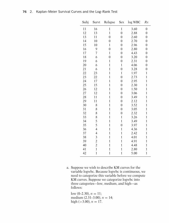
76 2. Kaplan–Meier Survival Curves and the Log–Rank Test
Subj Survt Relapse Sex log WBC Rx
11 16 1 1 3.60 012 13 1 0 2.88 013 11 0 0 2.60 014 10 0 0 2.70 015 10 1 0 2.96 016 9 0 0 2.80 017 7 1 0 4.43 018 6 0 0 3.20 019 6 1 0 2.31 020 6 1 1 4.06 021 6 1 0 3.28 022 23 1 1 1.97 123 22 1 0 2.73 124 17 1 0 2.95 125 15 1 0 2.30 126 12 1 0 1.50 127 12 1 0 3.06 128 11 1 0 3.49 129 11 1 0 2.12 130 8 1 0 3.52 131 8 1 0 3.05 132 8 1 0 2.32 133 8 1 1 3.26 134 5 1 1 3.49 135 5 1 0 3.97 136 4 1 1 4.36 137 4 1 1 2.42 138 3 1 1 4.01 139 2 1 1 4.91 140 2 1 1 4.48 141 1 1 1 2.80 142 1 1 1 5.00 1
a. Suppose we wish to describe KM curves for thevariable logwbc. Because logwbc is continuous, weneed to categorize this variable before we computeKM curves. Suppose we categorize logwbc intothree categories—low, medium, and high—asfollows:
low (0–2.30), n = 11;medium (2.31–3.00), n = 14;high (>3.00), n = 17.

Test 77
Based on this categorization, compute and graphKM curves for each of the three categories of logwbc.(You may use a computer program to assist you oryou can form three tables of ordered failure timesand compute KM probabilities directly.)
b. Compare the three KM plots you obtained in part a.How are they different?
c. Below is an edited printout of the log–rank testcomparing the three groups.
Events EventsGroup observed expected
1 4 13.062 10 10.723 16 6.21
Total 30 30.00
Log–rank = chi2(2) = 26.39P-value = Pr > chi2 = 0.0000
What do you conclude about whether or not thethree survival curves are the same?
Test To answer the questions below, you will need to use a com-puter program (from SAS, Stata, SPSS, or any other packageyou are familiar with) that computes and plots KM curves andcomputes the log–rank test. Freely downloadable files can beobtained from weblink http://www.sph.emory.edu/∼dkleinb/surv2.htm.
1. For the vets.dat data set described in the presentation:a. Obtain KM plots for the two categories of the
variable cell type 1 (1 = large, 0 = other). Commenton how the two curves compare with each other.Carry out the log–rank, and draw conclusions fromthe test(s).
b. Obtain KM plots for the four categories of celltype—large, adeno, small, and squamous. Note thatyou will need to recode the data to define a singlevariable which numerically distinguishes the fourcategories (e.g., 1 = large, 2 = adeno, etc.). As in parta, compare the four KM curves. Also, carry out thelog–rank for the equality of the four curves and drawconclusions.

78 2. Kaplan–Meier Survival Curves and the Log–Rank Test
2. The following questions consider a data set from a studyby Caplehorn et al. (“Methadone Dosage and Retention ofPatients in Maintenance Treatment,” Med. J. Aust., 1991).These data comprise the times in days spent by heroin ad-dicts from entry to departure from one of two methadoneclinics. There are two further covariates, namely, prisonrecord and methadone dose, believed to affect the sur-vival times. The data set name is addicts.dat. A listing ofthe variables is given below:
Column 1: Subject IDColumn 2: Clinic (1 or 2)Column 3: Survival status (0 = censored, 1 = departed
from clinic)Column 4: Survival time in daysColumn 5: Prison record (0 = none, 1 = any)Column 6: Methadone dose (mg/day)
a. Compute and plot the KM plots for the two categoriesof the “clinic” variable and comment on the extent towhich they differ.
b. A printout of the log–rank and Wilcoxon tests (usingStata) is provided below. What are your conclusionsfrom this printout?
Events EventsGroup observed expected
1 122 90.912 28 59.09
Total 150 150.00
Log–rank = chi2(2) = 27.89P-value = Pr > chi2 = 0.0000Wilcoxon = chi2(2) = 11.63P-value = Pr > chi2 = 0.0007
c. Compute and evaluate KM curves and the log–ranktest for comparing suitably chosen categories of thevariable “Methadone dose.” Explain how youdetermined the categories for this variable.
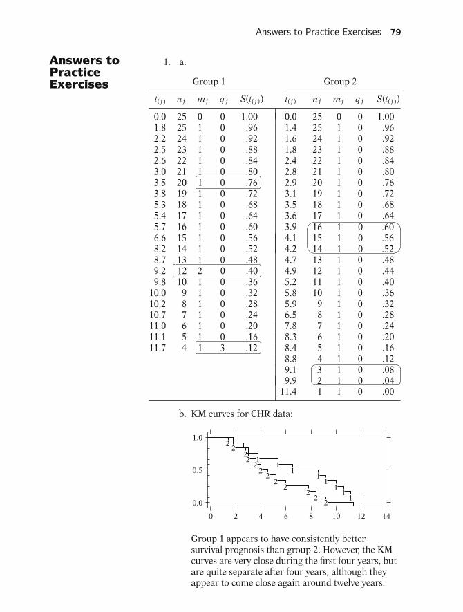
Answers to Practice Exercises 79
Answers toPracticeExercises
1. a.
Group 1 Group 2
t( j ) n j mj q j S(t( j )) t( j ) n j mj q j S(t( j ))
0.0 25 0 0 1.00 0.0 25 0 0 1.001.8 25 1 0 .96 1.4 25 1 0 .962.2 24 1 0 .92 1.6 24 1 0 .922.5 23 1 0 .88 1.8 23 1 0 .882.6 22 1 0 .84 2.4 22 1 0 .843.0 21 1 0 .80 2.8 21 1 0 .803.5 20
��
�1 0 .76 2.9 20 1 0 .76
3.8 19 1 0 .72 3.1 19 1 0 .725.3 18 1 0 .68 3.5 18 1 0 .685.4 17 1 0 .64 3.6 17 1 0 .645.7 16 1 0 .60 3.9
�
�
16 1 0 .6015 1 0 .5614 1 0 .52
6.6 15 1 0 .56 4.18.2 14 1 0 .52 4.28.7 13 1 0 .48 4.7 13 1 0 .489.2
��
�12 2 0 .40 4.9 12 1 0 .44
9.8 10 1 0 .36 5.2 11 1 0 .4010.0 9 1 0 .32 5.8 10 1 0 .3610.2 8 1 0 .28 5.9 9 1 0 .3210.7 7 1 0 .24 6.5 8 1 0 .2811.0 6 1 0 .20 7.8 7 1 0 .2411.1 5 1 0 .16 8.3 6 1 0 .2011.7 4
��
�1 3 .12 8.4 5 1 0 .16
8.8 4 1 0 .129.1
��
��
3 1 0 .082 1 0 .049.9
11.4 1 1 0 .00
b. KM curves for CHR data:
0.0
0.5
1.0
0 2 4 6 8 10 12 14
22
22
22
22
22
22
11
11
11
11
Group 1 appears to have consistently bettersurvival prognosis than group 2. However, the KMcurves are very close during the first four years, butare quite separate after four years, although theyappear to come close again around twelve years.

80 2. Kaplan–Meier Survival Curves and the Log–Rank Test
c. Using the expanded table format, the followinginformation is obtained:
t( j ) m1 j m2 j n1 j n2 j e1 j e2 j m1 j − e1 j m2 j − e2 j
1.4 0 1 25 25 .500 .500 −.500 .5001.6 0 1 25 24 .510 .490 −.510 .5101.8 1 1 25 23 1.042 .958 −.042 .0422.2 1 0 24 22 .522 .478 .478 −.4782.4. 0 1 23 22 .511 .489 −.511 .5112.5. 1 0 23 21 .523 .477 .477 −.4772.6 1 0 22 21 .516 .484 .484 −.4842.8 0 1 21 21 .500 .500 −.500 .5002.9 0 1 21 20 .512 .488 −.512 .5123.0 1 0 21 19 .525 .475 .475 −.4753.1
�
�
�
�
0 1 20 19 .513 .487 −.513 .5131 1 20 18 1.053 .947 −.053 .0530 1 19 17 .528 .472 −.528 .5281 0 19 16 .543 .457 .457 −.457
3.53.63.83.9 0 1 18 16 .529 .471 −.529 .5294.1 0 1 18 15 .545 .455 −.545 .5454.2 0 1 18 14 .563 .437 −.563 .5634.7 0 1 18 13 .581 .419 −.581 .5814.9 0 1 18 12 .600 .400 −.600 .6005.2 0 1 18 11 .621 .379 −.621 .6215.3 1 0 18 10 .643 .357 .357 −.3575.4 1 0 17 10 .630 .370 .370 −.3705.7 1 0 16 10 .615 .385 .385 −.3855.8 0 1 15 10 .600 .400 −.600 .6005.9 0 1 15 9 .625 .375 −.625 .6256.5 0 1 15 8 .652 .348 −.652 .6526.6 1 0 15 7 .682 .318 .318 −.3187.8 0 1 14 7 .667 .333 −.667 .6678.2 1 0 14 6 .700 .300 .300 −.3008.3 0 1 13 6 .684 .316 −.684 .6848.4 0 1 13 5 .722 .278 −.722 .7228.7 1 0 13 4 .765 .235 .335 −.3358.8 0 1 12 4 .750 .250 −.750 .7509.1 0 1 12 3 .800 .200 −.800 .8009.2
�
�
2 0 12 2 1.714 .286 .286 −.2861 0 10 2 .833 .167 .167 −.1670 1 9 2 .818 .182 −.818 .818
9.89.9
10.0 1 0 9 1 .900 .100 .100 −.10010.2 1 0 8 1 .888 .112 .112 −.11210.7 1 0 7 1 .875 .125 .125 −.12511.0 1 0 6 1 .857 .143 .143 −.14311.1 1 0 5 1 .833 .167 .167 −.16711.4 0 1 4 1 .800 .200 −.800 .80011.7 1 0 4 0 1.000 .000 .000 .000
Totals 22 25 30.79 16.21��
��−8.690 8.690
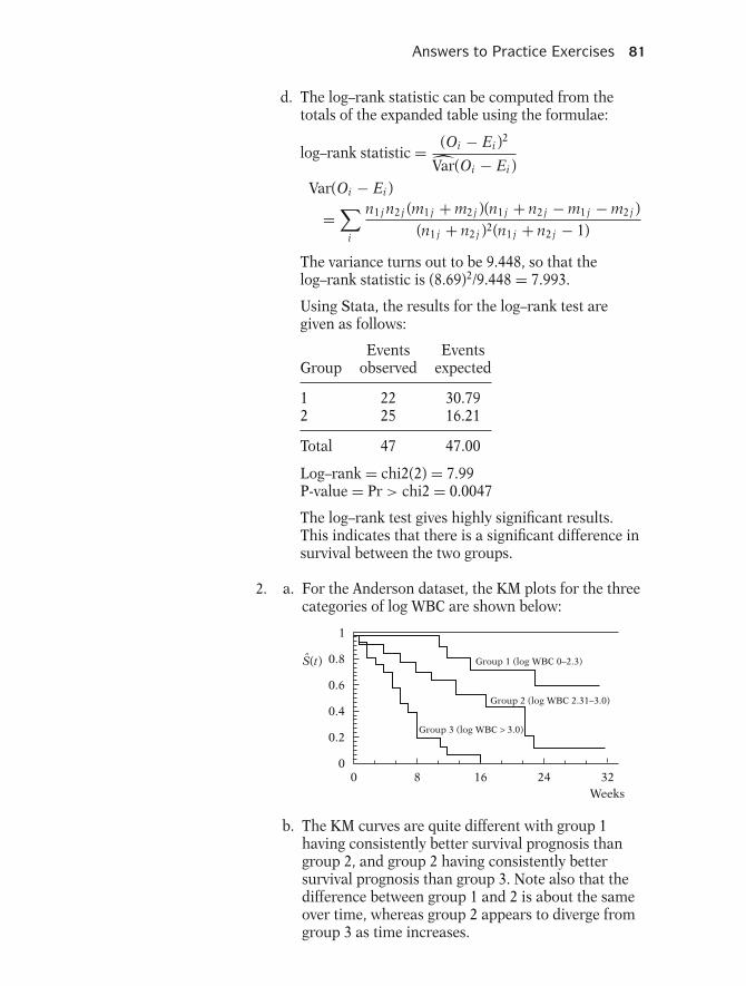
Answers to Practice Exercises 81
d. The log–rank statistic can be computed from thetotals of the expanded table using the formulae:
log–rank statistic = (Oi − Ei )2
Var(Oi − Ei )
Var(Oi − Ei )
=∑
i
n1 j n2 j (m1 j + m2 j )(n1 j + n2 j − m1 j − m2 j )(n1 j + n2 j )2(n1 j + n2 j − 1)
The variance turns out to be 9.448, so that thelog–rank statistic is (8.69)2/9.448 = 7.993.
Using Stata, the results for the log–rank test aregiven as follows:
Events EventsGroup observed expected
1 22 30.792 25 16.21
Total 47 47.00
Log–rank = chi2(2) = 7.99P-value = Pr > chi2 = 0.0047
The log–rank test gives highly significant results.This indicates that there is a significant difference insurvival between the two groups.
2. a. For the Anderson dataset, the KM plots for the threecategories of log WBC are shown below:
Group 1 (log WBC 0–2.3)
Group 2 (log WBC 2.31–3.0)
Group 3 (log WBC > 3.0)
00
0.2
0.4
0.6
0.8
1
8 16 24 32Weeks
S(t)
b. The KM curves are quite different with group 1having consistently better survival prognosis thangroup 2, and group 2 having consistently bettersurvival prognosis than group 3. Note also that thedifference between group 1 and 2 is about the sameover time, whereas group 2 appears to diverge fromgroup 3 as time increases.
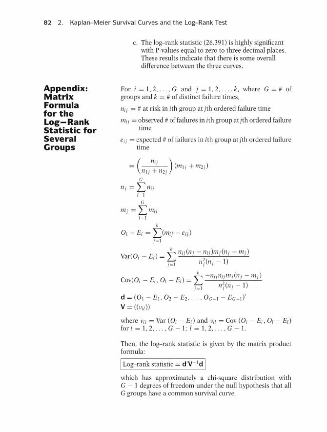
82 2. Kaplan–Meier Survival Curves and the Log–Rank Test
c. The log–rank statistic (26.391) is highly significantwith P-values equal to zero to three decimal places.These results indicate that there is some overalldifference between the three curves.
Appendix:MatrixFormulafor theLog-RankStatistic forSeveralGroups
For i = 1, 2, . . . , G and j = 1, 2, . . . , k, where G = # ofgroups and k = # of distinct failure times,
ni j = # at risk in ith group at jth ordered failure time
mi j = observed # of failures in ith group at jth ordered failuretime
ei j = expected # of failures in ith group at jth ordered failuretime
=(
ni j
n1 j + n2 j
)(m1 j + m2 j )
n j =G∑
i=1
ni j
mj =G∑
i=1
mi j
Oi − Ei =k∑
j=1
(mi j − ei j )
Var(Oi − Ei ) =k∑
j=1
ni j (n j − ni j )mj (n j − mj )
n2j (n j − 1)
Cov(Oi − Ei , Ol − El ) =k∑
j=1
−ni j nl j mj (n j − mj )
n2j (n j − 1)
d = (O1 − E1, O2 − E2, . . . , OG−1 − EG−1)′
V = ((νil ))
where νii = Var (Oi − Ei ) and νil = Cov (Oi − Ei , Ol − El )for i = 1, 2, . . . , G − 1; l = 1, 2, . . . , G − 1.
Then, the log–rank statistic is given by the matrix productformula:
Log–rank statistic = d′V−1d
which has approximately a chi-square distribution withG − 1 degrees of freedom under the null hypothesis that allG groups have a common survival curve.

3 The CoxProportionalHazardsModel andIts Charact-eristics
83

84 3. The Cox Proportional Hazards Model and Its Characteristics
Introduction We begin by discussing some computer results using the CoxPH model, without actually specifying the model; the purposehere is to show the similarity between the Cox model andstandard linear regression or logistic regression.
We then introduce the Cox model and describe why it is sopopular. In addition, we describe its basic properties, includ-ing the meaning of the proportional hazards assumption andthe Cox likelihood.
AbbreviatedOutline
The outline below gives the user a preview of the material tobe covered by the presentation. A detailed outline for reviewpurposes follows the presentation.
I. A computer example using the Cox PH model(pages 86–94)
II. The formula for the Cox PH model (pages 94–96)III. Why the Cox PH model is popular (pages 96–98)IV. ML estimation of the Cox PH model
(pages 98–100)V. Computing the hazard ratio (pages 100–103)
VI. Adjusted survival curves using the Cox PH model(pages 103–107)
VII. The meaning of the PH assumption(pages 107–111)
VIII. The Cox likelihood (pages 111–115)IX. Summary (pages 115–116)

Objectives 85
Objectives Upon completing this chapter, the learner should be able to:
1. State or recognize the general form of the Cox PH model.2. State the specific form of a Cox PH model appropriate for
the analysis, given a survival analysis scenario involvingone or more explanatory variables.
3. State or recognize the form and properties of the baselinehazard function in the Cox PH model.
4. Give three reasons for the popularity of the Cox PHmodel.
5. State the formula for a designated hazard ratio of interestgiven a scenario describing a survival analysis using aCox PH model, whena. there are confounders but no interaction terms in the
model;b. there are both confounders and interaction terms in
the model.6. State or recognize the meaning of the PH assumption.7. Determine and explain whether the PH assumption is
satisfied when the graphs of the hazard functions for twogroups cross each other over time.
8. State or recognize what is an adjusted survival curve.9. Compare and/or interpret two or more adjusted survival
curves.10. Given a computer printout involving one or more fitted
Cox PH models,a. compute or identify any hazard ratio(s) of interest;b. carry out and interpret a designated test of
hypothesis;c. carry out, identify or interpret a confidence interval
for a designated hazard ratio;d. evaluate interaction and confounding involving one
or more covariates.11. Give an example of how the Cox PH likelihood is formed.

86 3. The Cox Proportional Hazards Model and Its Characteristics
Presentation
FOCUS
• model form• why popular• ML estimation• hazard ratio• adjusted survival curves• PH assumption
This presentation describes the Cox proportionalhazards (PH) model, a popular mathematicalmodel used for analyzing survival data. Here, wefocus on the model form, why the model is pop-ular, maximum likelihood (ML) estimation of themodel parameters, the formula for the hazard ra-tio, how to obtain adjusted survival curves, andthe meaning of the PH assumption.
I. A Computer Example Usingthe Cox PH Model We introduce the Cox PH model using computer
output from the analysis of remission time data(Freireich et al., Blood, 1963), which we previouslydiscussed in Chapters 1 and 2. The data set is listedhere at the left.
These data involve two groups of leukemia pa-tients, with 21 patients in each group. Group 1is the treatment group, and group 2 is the placebogroup. The data set also contains the variable logWBC, which is a well-known prognostic indicatorof survival for leukemia patients.
For this example, the basic question of interestconcerns comparing the survival experience of thetwo groups adjusting for the possible confoundingand/or interaction effects of log WBC.
Group 1(n = 21) Group 2(n = 21)
6 2.31
6 4.06
6 3.28
7 4.43
10 2.96
13 2.88
16 3.60
22 2.32
23 2.57
6+ 3.20
9+ 2.80
10+ 2.70
11+ 2.60
17+ 2.16
19+ 2.05
20+ 2.01
25+ 1.78
32+ 2.20
32+ 2.53
34+ 1.47
35+ 1.45
1 2.80
1 5.00
2 4.91
2 4.48
3 4.01
4 4.36
4 2.42
5 3.49
5 3.97
8 3.52
8 3.05
8 2.32
8 3.26
11 3.49
11 2.12
12 1.50
12 3.06
15 2.30
17 2.95
22 2.73
23 1.97
Leukemia Remission Data
+ denotes censored observation
EXAMPLE
t(weeks) log WBC t(weeks) log WBC
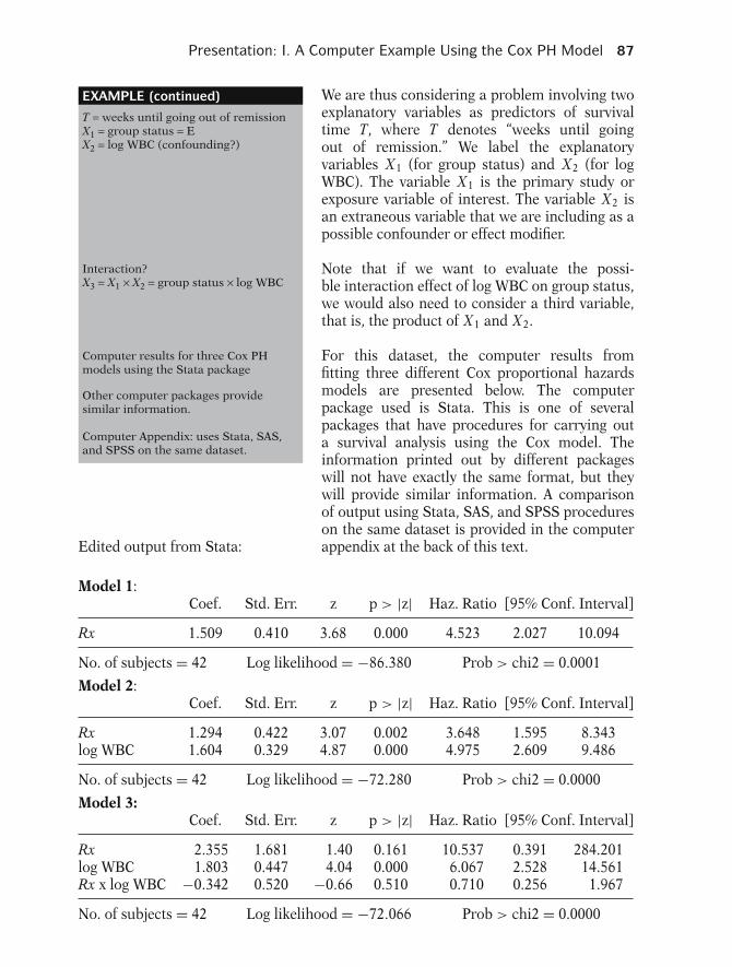
Presentation: I. A Computer Example Using the Cox PH Model 87
EXAMPLE (continued)
T = weeks until going out of remissionX1 = group status = EX2 = log WBC (confounding?)
Interaction?X3 = X1 × X2 = group status × log WBC
Computer results for three Cox PHmodels using the Stata package
Other computer packages providesimilar information.
Computer Appendix: uses Stata, SAS,and SPSS on the same dataset.
We are thus considering a problem involving twoexplanatory variables as predictors of survivaltime T, where T denotes “weeks until goingout of remission.” We label the explanatoryvariables X1 (for group status) and X2 (for logWBC). The variable X1 is the primary study orexposure variable of interest. The variable X2 isan extraneous variable that we are including as apossible confounder or effect modifier.
Note that if we want to evaluate the possi-ble interaction effect of log WBC on group status,we would also need to consider a third variable,that is, the product of X1 and X2.
For this dataset, the computer results fromfitting three different Cox proportional hazardsmodels are presented below. The computerpackage used is Stata. This is one of severalpackages that have procedures for carrying outa survival analysis using the Cox model. Theinformation printed out by different packageswill not have exactly the same format, but theywill provide similar information. A comparisonof output using Stata, SAS, and SPSS procedureson the same dataset is provided in the computerappendix at the back of this text.Edited output from Stata:
Model 1:Coef. Std. Err. z p > |z| Haz. Ratio [95% Conf. Interval]
Rx 1.509 0.410 3.68 0.000 4.523 2.027 10.094
No. of subjects = 42 Log likelihood = −86.380 Prob > chi2 = 0.0001
Model 2:Coef. Std. Err. z p > |z| Haz. Ratio [95% Conf. Interval]
Rx 1.294 0.422 3.07 0.002 3.648 1.595 8.343log WBC 1.604 0.329 4.87 0.000 4.975 2.609 9.486
No. of subjects = 42 Log likelihood = −72.280 Prob > chi2 = 0.0000
Model 3:Coef. Std. Err. z p > |z| Haz. Ratio [95% Conf. Interval]
Rx 2.355 1.681 1.40 0.161 10.537 0.391 284.201log WBC 1.803 0.447 4.04 0.000 6.067 2.528 14.561Rx x log WBC −0.342 0.520 −0.66 0.510 0.710 0.256 1.967
No. of subjects = 42 Log likelihood = −72.066 Prob > chi2 = 0.0000
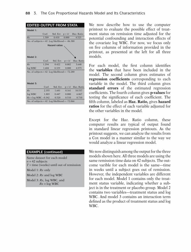
88 3. The Cox Proportional Hazards Model and Its Characteristics
EDITED OUTPUT FROM STATAModel 1:
Coef. Std. Err. p > |z| Haz. Ratio
Rx 1.509 0.410 0.000 4.523
No. of subjects = 42 Log likelihood = −86.380
Hazard ratios
Model 2:
Coef. Std. Err. p > |z| Haz. Ratio
Rx 1.294 0.422 0.002 3.648
log WBC 1.604 0.329 0.000 4.975
No. of subjects = 42 Log likelihood = −72.280
Model 3: Coef. Std. Err. p > |z| Haz. Ratio
Rx 2.355 1.681 0.161 10.537
Rx × log WBC −0.342 0.520 0.510 0.710
log WBC 1.803 0.447 0.000 6.067
No. of subjects = 42 Log likelihood = −72.066
We now describe how to use the computerprintout to evaluate the possible effect of treat-ment status on remission time adjusted for thepotential confounding and interaction effects ofthe covariate log WBC. For now, we focus onlyon five columns of information provided in theprintout, as presented at the left for all threemodels.
For each model, the first column identifiesthe variables that have been included in themodel. The second column gives estimates ofregression coefficients corresponding to eachvariable in the model. The third column givesstandard errors of the estimated regressioncoefficients. The fourth column gives p-values fortesting the significance of each coefficient. Thefifth column, labeled as Haz. Ratio, gives hazardratios for the effect of each variable adjusted forthe other variables in the model.
Except for the Haz. Ratio column, thesecomputer results are typical of output foundin standard linear regression printouts. As theprintout suggests, we can analyze the results froma Cox model in a manner similar to the way wewould analyze a linear regression model.
EXAMPLE (continued)
Same dataset for each modeln = 42 subjectsT = time (weeks) until out of remission
Model 1: Rx only
Model 2: Rx and log WBC
Model 3: Rx, log WBC, andRx × log WBC
We now distinguish among the output for the threemodels shown here. All three models are using thesame remission time data on 42 subjects. The out-come varible for each model is the same—timein weeks until a subject goes out of remission.However, the independent variables are differentfor each model. Model 1 contains only the treat-ment status variable, indicating whether a sub-ject is in the treatment or placebo group. Model 2contains two variables—treatment status and logWBC. And model 3 contains an interaction termdefined as the product of treatment status and logWBC.
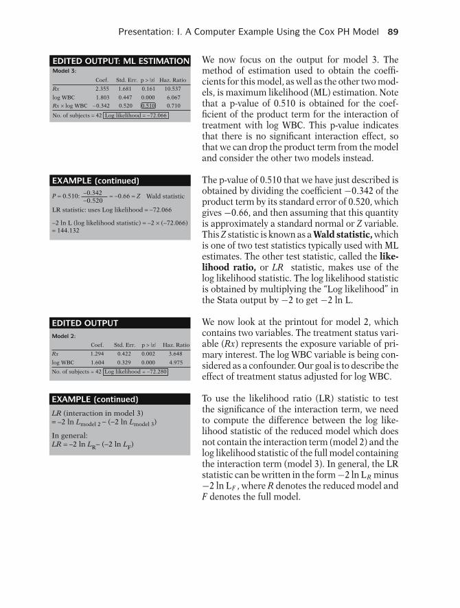
Presentation: I. A Computer Example Using the Cox PH Model 89
EDITED OUTPUT: ML ESTIMATIONModel 3:
Coef. Std. Err. p > |z| Haz. Ratio
Rx 2.355 1.681 0.161 10.537
Rx × log WBC −0.342 0.520 0.510 0.710
log WBC 1.803 0.447 0.000 6.067
No. of subjects = 42 Log likelihood = −72.066
We now focus on the output for model 3. Themethod of estimation used to obtain the coeffi-cients for this model, as well as the other two mod-els, is maximum likelihood (ML) estimation. Notethat a p-value of 0.510 is obtained for the coef-ficient of the product term for the interaction oftreatment with log WBC. This p-value indicatesthat there is no significant interaction effect, sothat we can drop the product term from the modeland consider the other two models instead.
EXAMPLE (continued)
P = 0.510: = −0.66 = Z−0.342−0.520
Wald statistic
LR statistic: uses Log likelihood = −72.066
−2 ln L (log likelihood statistic) = −2 × (−72.066)= 144.132
The p-value of 0.510 that we have just described isobtained by dividing the coefficient −0.342 of theproduct term by its standard error of 0.520, whichgives −0.66, and then assuming that this quantityis approximately a standard normal or Z variable.This Z statistic is known as a Wald statistic, whichis one of two test statistics typically used with MLestimates. The other test statistic, called the like-lihood ratio, or LR statistic, makes use of thelog likelihood statistic. The log likelihood statisticis obtained by multiplying the “Log likelihood” inthe Stata output by −2 to get −2 ln L.
EDITED OUTPUT Model 2:
Coef. Std. Err. p > |z| Haz. Ratio
Rx 1.294 0.422 0.002 3.648
log WBC 1.604 0.329 0.000 4.975
No. of subjects = 42 Log likelihood = −72.280
We now look at the printout for model 2, whichcontains two variables. The treatment status vari-able (Rx) represents the exposure variable of pri-mary interest. The log WBC variable is being con-sidered as a confounder. Our goal is to describe theeffect of treatment status adjusted for log WBC.
EXAMPLE (continued)
LR (interaction in model 3)= –2 ln Lmodel 2 − (−2 ln Lmodel 3)
In general:LR = –2 ln LR− (−2 ln LF)
To use the likelihood ratio (LR) statistic to testthe significance of the interaction term, we needto compute the difference between the log like-lihood statistic of the reduced model which doesnot contain the interaction term (model 2) and thelog likelihood statistic of the full model containingthe interaction term (model 3). In general, the LRstatistic can be written in the form −2 ln LR minus−2 ln LF , where R denotes the reduced model andF denotes the full model.
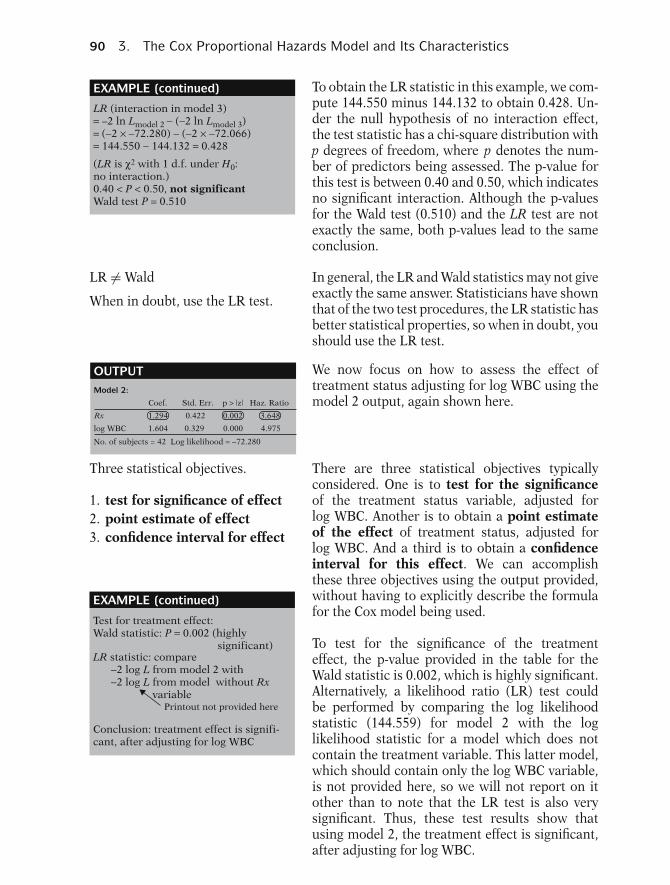
90 3. The Cox Proportional Hazards Model and Its Characteristics
EXAMPLE (continued)
LR (interaction in model 3)= –2 ln Lmodel 2 − (−2 ln Lmodel 3)= (−2 × −72.280) − (−2 × −72.066)= 144.550 − 144.132 = 0.428
(LR is χ2 with 1 d.f. under H0:no interaction.)0.40 < P < 0.50, not significantWald test P = 0.510
To obtain the LR statistic in this example, we com-pute 144.550 minus 144.132 to obtain 0.428. Un-der the null hypothesis of no interaction effect,the test statistic has a chi-square distribution withp degrees of freedom, where p denotes the num-ber of predictors being assessed. The p-value forthis test is between 0.40 and 0.50, which indicatesno significant interaction. Although the p-valuesfor the Wald test (0.510) and the LR test are notexactly the same, both p-values lead to the sameconclusion.
LR �= Wald
When in doubt, use the LR test.
In general, the LR and Wald statistics may not giveexactly the same answer. Statisticians have shownthat of the two test procedures, the LR statistic hasbetter statistical properties, so when in doubt, youshould use the LR test.
OUTPUTModel 2:
Coef. Std. Err. p > |z| Haz. Ratio
Rx 1.294 0.422 0.002 3.648
log WBC 1.604 0.329 0.000 4.975
No. of subjects = 42 Log likelihood = −72.280
We now focus on how to assess the effect oftreatment status adjusting for log WBC using themodel 2 output, again shown here.
Three statistical objectives.
1. test for significance of effect2. point estimate of effect3. confidence interval for effect
EXAMPLE (continued)
Test for treatment effect: Wald statistic: P = 0.002 (highly
significant)LR statistic: compare
−2 log L from model 2 with −2 log L from model without Rx
variablePrintout not provided here
Conclusion: treatment effect is signifi- cant, after adjusting for log WBC
There are three statistical objectives typicallyconsidered. One is to test for the significanceof the treatment status variable, adjusted forlog WBC. Another is to obtain a point estimateof the effect of treatment status, adjusted forlog WBC. And a third is to obtain a confidenceinterval for this effect. We can accomplishthese three objectives using the output provided,without having to explicitly describe the formulafor the Cox model being used.
To test for the significance of the treatmenteffect, the p-value provided in the table for theWald statistic is 0.002, which is highly significant.Alternatively, a likelihood ratio (LR) test couldbe performed by comparing the log likelihoodstatistic (144.559) for model 2 with the loglikelihood statistic for a model which does notcontain the treatment variable. This latter model,which should contain only the log WBC variable,is not provided here, so we will not report on itother than to note that the LR test is also verysignificant. Thus, these test results show thatusing model 2, the treatment effect is significant,after adjusting for log WBC.

Presentation: I. A Computer Example Using the Cox PH Model 91
EXAMPLE (continued)
Point estimate:
Coefficient of treatment variable
HR = 3.648= e1.294
ˆ
A point estimate of the effect of the treatment isprovided in the HR column by the value 3.648.This value gives the estimated hazard ratio (HR)for the effect of the treatment; in particular,we see that the hazard for the placebo group is3.6 times the hazard for the treatment group.Note that the value 3.648 is calculated as e to thecoefficient of the treatment variable; that is, e tothe 1.294 equals 3.648.
To describe the confidence interval for the ef-fect of treatment status, we consider the outputfor the extended table for model 2 given earlier.
Model 2:[95% Conf. Interval]
3.07
log WBC
No. of subjects = 42 Log likelihood = −72.280 Prob > chi2 = 0.0000
OUTPUT
Coef.
1.595 8.343 1.294Rx
4.87 2.609 9.4861.604
3.648
4.975
z Haz. Ratiop > |z|
0.002
0.000
0.422
0.329
Std. Err.
95% confidence interval for the HR:(1.595, 8.343)
95% CI for β1: 1.294 ± (1.96) (0.422)
95% CI for HR = eβ1:
1(
1.595 3.648 8.343
0 1.96 Z
exp[β1 ± 1.96sβ1] = e1.294 ± 1.96(0.422)
EXAMPLE (continued)
0.975
)
From the table, we see that a 95% confidenceinterval for the treatment effect is given by therange of values 1.595–8.343. This is a confidenceinterval for the hazard ratio (HR), which sur-rounds the point estimate of 3.648 previouslydescribed. Notice that this confidence interval isfairly wide, indicating that the point estimate issomewhat unreliable. As expected from the lowp-value of 0.002, the confidence interval for HRdoes not contain the null value of 1.
The calculation of the confidence intervalfor HR is carried out as follows:
1. Compute a 95% confidence interval for the re-gression coefficient of the Rx variable (β1). Thelarge sample formula is 1.294 plus or minus1.96 times the standard error 0.422, where 1.96is the 97.5 percentile of the standard normal orZ distribution.
2. Exponentiate the two limits obtained for theconfidence interval for the regression coeffi-cient of Rx.

92 3. The Cox Proportional Hazards Model and Its Characteristics
Stata: provides CI directly
Other packages: provide β’s and sβ
’s
The Stata output provides the required confidenceinterval directly, so that the user does not have tocarry out the computations required by the largesample formula. Other computer packages maynot provide the confidence interval directly, but,rather, may provide only the estimated regressioncoefficients and their standard errors.
EDITED OUTPUTModel 1:
Coef. Std. Err. p > |z| Haz. Ratio
Rx 1.509 0.410 0.000 4.523
No. of subjects = 42 Log likelihood = −86.380
Model 2:
Coef. Std. Err. p > |z| Haz. Ratio
Rx 1.294 0.422 0.002 3.648
log WBC 1.604 0.329 0.000 4.975
No. of subjects = 42 Log likelihood = −72.280
To this point, we have made use of informationfrom outputs for models 2 and 3, but have not yetconsidered the model 1 output, which is shownagain here. Note that model 1 contains only thetreatment status variable, whereas model 2, shownbelow, contains log WBC in addition to treatmentstatus. Model 1 is sometimes called the “crude”model because it ignores the effect of potential co-variates of interest, like log WBC.
EXAMPLE (continued)
ˆ
HR for model 1 (4.523) is higher than HR for model 2 (3.648).
Confounding: crude versus adjustedHR’s are meaningfully different.
Confounding due to log WBC ⇒ must control for log WBC, i.e., prefer model 2 to model 1.
If no confounding, then consider preci- sion: e.g., if 95% CI is narrower for model 2 than model 1, we prefer model 2.
Model 1 can be used in comparison with model 2to evaluate the potential confounding effect of thevariable log WBC. In particular, notice that thevalue in the HR column for the treatment statusvariable is 4.523 for model 1, but only 3.648 formodel 2. Thus, the crude model yields an esti-mated hazard ratio that is somewhat higher thanthe corresponding estimate obtained when we ad-just for log WBC. If we decide that the crude andadjusted estimates are meaningfully different, wethen say that there is confounding due to log WBC.
Once we decide that confounding is present, wethen must control for the confounder—in thiscase, log WBC—in order to obtain a valid estimateof the effect. Thus, we prefer model 2, whichcontrols for log WBC, to model 1, which does not.
Note that if we had decided that there is no “mean-ingful” confounding, then we would not need tocontrol for log WBC to get a valid answer. Nev-ertheless, we might wish to control for log WBCanyhow, to obtain a more precise estimate of thehazard ratio. That is, if the confidence interval forthe HR is narrower when using model 2 than whenusing model 1, we would prefer model 2 to model 1for precision gain.
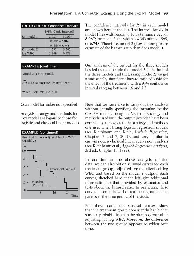
Presentation: I. A Computer Example Using the Cox PH Model 93
EDITED OUTPUT: Confidence Intervals
[95% Conf. Interval]
Rx model 1 2.027 10.094
Rx model 2 1.595 8.343log WBC 2.609 9.486
width = 8.067
width = 6.748
The confidence intervals for Rx in each modelare shown here at the left. The interval for Rx inmodel 1 has width equal to 10.094 minus 2.027, or8.067; for model 2, the width is 8.343 minus 1.595,or 6.748. Therefore, model 2 gives a more preciseestimate of the hazard ratio than does model 1.
EXAMPLE (continued)
Model 2 is best model.
HR = 3.648 statistically significantˆ95% CI for HR: (1.6, 8.3)
Our analysis of the output for the three modelshas led us to conclude that model 2 is the best ofthe three models and that, using model 2, we geta statistically significant hazard ratio of 3.648 forthe effect of the treatment, with a 95% confidenceinterval ranging between 1.6 and 8.3.
Cox model formulae not specified
Analysis strategy and methods forCox model analogous to those forlogistic and classical linear models.
EXAMPLE (continued)Survival Curves Adjusted for log WBC(Model 2)
1.0
.8
.6
.4
.2
.08 16 24
Placebo(Rx = 1)
Treatment (Rx = 0)
Time
S(t)
Note that we were able to carry out this analysiswithout actually specifying the formulae for theCox PH models being fit. Also, the strategy andmethods used with the output provided have beencompletely analogous to the strategy and methodsone uses when fitting logistic regression models(see Kleinbaum and Klein, Logistic Regression,Chapters 6 and 7, 2002), and very similar tocarrying out a classical linear regression analysis(see Kleinbaum et al., Applied Regression Analysis,3rd ed., Chapter 16, 1997).
In addition to the above analysis of thisdata, we can also obtain survival curves for eachtreatment group, adjusted for the effects of logWBC and based on the model 2 output. Suchcurves, sketched here at the left, give additionalinformation to that provided by estimates andtests about the hazard ratio. In particular, thesecurves describe how the treatment groups com-pare over the time period of the study.
For these data, the survival curves showthat the treatment group consistently has highersurvival probabilities than the placebo group afteradjusting for log WBC. Moreover, the differencebetween the two groups appears to widen overtime.

94 3. The Cox Proportional Hazards Model and Its Characteristics
Adjusted survivalcurves KM curvesAdjusted for No covariatescovariatesUse fitted Cox No Cox modelmodel fitted
Note that adjusted survival curves are mathemat-ically different from Kaplan–Meier (KM) curves.KM curves do not adjust for covariates and, there-fore, are not computed using results from a fittedCox PH model.
Nevertheless, for these data, the plotted KM curves(which were described in Chapter 2) are similar inappearance to the adjusted survival curves.
Remainder:
� Cox model formula� basic characteristics of Coxmodel� meaning of PH assumption
In the remainder of this presentation, we describethe Cox PH formula and its basic characteristics,including the meaning of the PH assumption andthe Cox likelihood.
II. The Formula for theCox PH Model
h(t, X) = h0(t) e
p∑i=1
βi Xi
X = (X1, X2, . . . , X p)explanatory/predictor variables
The Cox PH model is usually written in termsof the hazard model formula shown here at theleft. This model gives an expression for the hazardat time t for an individual with a given specifica-tion of a set of explanatory variables denoted bythe bold X. That is, the bold X represents a col-lection (sometimes called a “vector”) of predictorvariables that is being modeled to predict an indi-vidual’s hazard.
h0(t) × e
p∑i=1
βi Xi
Baseline ExponentialhazardInvolves t Involves X ’s butbut not not t (X’s areX ’s time-independent)
The Cox model formula says that the hazard attime t is the product of two quantities. The firstof these, h0(t), is called the baseline hazardfunction. The second quantity is the exponentialexpression e to the linear sum of βi Xi , where thesum is over the p explanatory X variables.
An important feature of this formula, whichconcerns the proportional hazards (PH) assump-tion, is that the baseline hazard is a function oft, but does not involve the X ’s. In contrast, theexponential expression shown here, involves theX ’s, but does not involve t. The X ’s here are calledtime-independent X ’s.

Presentation: II. The Formula for the Cox PH Model 95
X ’s involving t: time-dependent
Requires extended Cox model (noPH)
It is possible, nevertheless, to consider X ’s whichdo involve t. Such X ’s are called time-dependentvariables. If time-dependent variables are consid-ered, the Cox model form may still be used, butsuch a model no longer satisfies the PH assump-tion, and is called the extended Cox model.
Time-dependent variables:Chapter 6
The use of time-dependent variables is discussedin Chapter 6. For the remainder of this presenta-tion, we will consider time-independent X ’s only.
Time-independent variable:Values for a given individualdo not change over time; e.g.,SEX and SMK↘
Assumed not to changeonce measured
A time-independent variable is defined to be anyvariable whose value for a given individual doesnot change over time. Examples are SEX andsmoking status (SMK). Note, however, that a per-son’s smoking status may actually change overtime, but for purposes of the analysis, the SMKvariable is assumed not to change once it is mea-sured, so that only one value per individual is used.
AGE and WGT values do not changemuch, or effect on survival dependson one measurement.
Also note that although variables like AGE andweight (WGT) change over time, it may be appro-priate to treat such variables as time-independentin the analysis if their values do not change muchover time or if the effect of such variables on sur-vival risk depends essentially on the value at onlyone measurement.
X1 = X2 = · · · = X p = 0
h(t,X) = h0(t) e
p∑i=1
βi Xi
= h0(t) e0
= h0(t)Baseline hazard
The Cox model formula has the property that ifall the X ’s are equal to zero, the formula reducesto the baseline hazard function. That is, the expo-nential part of the formula becomes e to the zero,which is 1. This property of the Cox model is thereason why h0(t) is called the baseline function.
No X ’s in model: h(t,X) = h0(t). Or, from a slightly different perspective, the Coxmodel reduces to the baseline hazard when no X ’sare in the model. Thus, h0(t) may be consideredas a starting or “baseline” version of the hazardfunction, prior to considering any of the X ’s.
h0(t) is unspecified.
Cox model: semiparametric
Another important property of the Cox model isthat the baseline hazard, h0(t), is an unspecifiedfunction. It is this property that makes the Coxmodel a semiparametric model.

96 3. The Cox Proportional Hazards Model and Its Characteristics
EXAMPLE: Parametric Model
Weibull:h(t, X) = λptp–1
and h0(t) = ptp–1
p
where λ = exp[ΣβiXi]i=1
In contrast, a parametric model is one whosefunctional form is completely specified, except forthe values of the unknown parameters. For ex-ample, the Weibull hazard model is a parametricmodel and has the form shown here, where theunknown parameters are λ, p, and the βi ’s. Notethat for the Weibull model, h0(t) is given by λptp−1
(see Chapter 7).
Semiparametric property⇓
Popularity of the Cox model
One of the reasons why the Cox model is so popu-lar is that it is semiparametric. We discuss this andother reasons in the next section (III) concerningwhy the Cox model is so widely used.
III. Why the Cox PH ModelIs Popular
Cox PH model is “robust”: Willclosely approximate correctparametric model
A key reason for the popularity of the Cox model isthat, even though the baseline hazard is not spec-ified, reasonably good estimates of regression co-efficients, hazard ratios of interest, and adjustedsurvival curves can be obtained for a wide varietyof data situations. Another way of saying this isthat the Cox PH model is a “robust” model, so thatthe results from using the Cox model will closelyapproximate the results for the correct parametricmodel.
If correct model is:
Cox model willWeibull ⇒ approximate
Weibull
Cox model willExponential ⇒ approximate
exponential
For example, if the correct parametric model isWeibull, then use of the Cox model typically willgive results comparable to those obtained using aWeibull model. Or, if the correct model is expo-nential, then the Cox model results will closely ap-proximate the results from fitting an exponentialmodel.
Prefer parametric model if sure ofcorrect model, e.g., use goodness-of-fit test (Lee, 1982).
We would prefer to use a parametric model if wewere sure of the correct model. Although there arevarious methods for assessing goodness of fit of aparametric model (for example, see Lee, StatisticalMethods for Survival Data Analysis, 1982), we maynot be completely certain that a given parametricmodel is appropriate.

Presentation: III. Why the Cox PH Model Is Popular 97
When in doubt, the Cox model is a“safe” choice.
Thus, when in doubt, as is typically the case, theCox model will give reliable enough results so thatit is a “safe” choice of model, and the user doesnot need to worry about whether the wrong para-metric model is chosen.
In addition to the general “robustness” of the Coxmodel, the specific form of the model is attractivefor several reasons.
h(t,X) = h0(t) × e
p∑i=1
βi Xi
Baseline Exponentialhazard ⇓
0 ≤ h(t,X) < ∞ always
As described previously, the specific form of theCox model gives the hazard function as a productof a baseline hazard involving t and an exponentialexpression involving the X ’s without t. The expo-nential part of this product is appealing becauseit ensures that the fitted model will always giveestimated hazards that are non-negative.
h0(t) ×p∑
i=1
βi Xi︸ ︷︷ ︸Linear
⇓Might be < 0
We want such nonnegative estimates because, bydefinition, the values of any hazard function mustrange between zero and plus infinity, that is, a haz-ard is always nonnegative. If, instead of an expo-nential expression, the X part of the model were,for example, linear in the X ’s, we might obtain neg-ative hazard estimates, which are not allowed.
Even though h0(t) is unspecified,we can estimate the β’s.
Measure of effect: hazard ratio (HR)involves only β’s, withoutestimating h0(t).
Another appealing property of the Cox model isthat, even though the baseline hazard part of themodel is unspecified, it is still possible to estimatethe β’s in the exponential part of the model. Aswe will show later, all we need are estimates of theβ’s to assess the effect of explanatory variables ofinterest. The measure of effect, which is called ahazard ratio, is calculated without having to esti-mate the baseline hazard function.
Can estimate h(t,X) and S(t,X)for Cox model using a minimumof assumptions.
Note that the hazard function h(t,X) and its corre-sponding survival curves S(t,X) can be estimatedfor the Cox model even though the baseline haz-ard function is not specified. Thus, with the Coxmodel, using a minimum of assumptions, we canobtain the primary information desired from asurvival analysis, namely, a hazard ratio and a sur-vival curve.

98 3. The Cox Proportional Hazards Model and Its Characteristics
Cox model preferred to logistic model.⇓ ⇓Uses survival Uses (0,1) outcome;times and ignores survival timescensoring and censoring
One last point about the popularity of the Coxmodel is that it is preferred over the logistic modelwhen survival time information is available andthere is censoring. That is, the Cox model usesmore information—the survival times—than thelogistic model, which considers a (0,1) outcomeand ignores survival times and censoring.
IV. ML Estimation of theCox PH Model
h(t, X) = h0(t) e
p∑i=1
βi Xi
We now describe how estimates are obtained forthe parameters of the Cox model. The parame-ters are the β’s in the general Cox model formulashown here. The corresponding estimates of theseparameters are called maximum likelihood (ML)estimates and are denoted as βi “hat.”
ML estimates: β i
Coef. Std.Err. p > |z| Haz. RatioRx 1.294 0.422 0.002 3.648log WBC 1.604 0.329 0.000 4.975�No. of subjects = 42 Log likelihood = −72.280
Estimated model:h(t,X) = h0(t)e1.294 Rx + 1.604 log WBC
As an example of ML estimates, we consider onceagain the computer output for one of the models(model 2) fitted previously from remission dataon 42 eukemia patients.
The Cox model for this example involvestwo parameters, one being the coefficient ofthe treatment variable (denoted here as Rx)and the other being the coefficient of the logWBC variable. The expression for this model isshown at the left, which contains the estimatedcoefficients 1.294 for Rx and 1.604 for log whiteblood cell count.
ML estimates: maximize likelihoodfunction L
L = joint probability of observeddata = L(β)
As with logistic regression, the ML estimates ofthe Cox model parameters are derived by maxi-mizing a likelihood function, usually denoted asL. The likelihood function is a mathematical ex-pression which describes the joint probability ofobtaining the data actually observed on the sub-jects in the study as a function of the unknown pa-rameters (the β’s) in the model being considered.L is sometimes written notationally as L(β) whereβ denotes the collection of unknown parameters.
The expression for the likelihood is developed atthe end of the chapter. However, we give a briefoverview below.
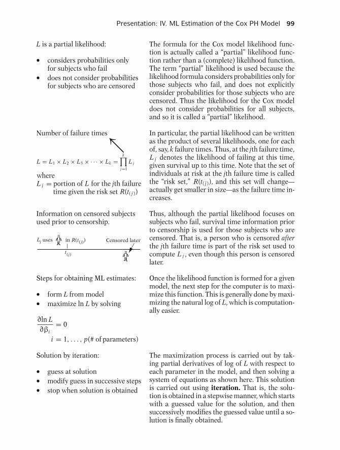
Presentation: IV. ML Estimation of the Cox PH Model 99
L is a partial likelihood:
� considers probabilities onlyfor subjects who fail� does not consider probabilitiesfor subjects who are censored
The formula for the Cox model likelihood func-tion is actually called a “partial” likelihood func-tion rather than a (complete) likelihood function.The term “partial” likelihood is used because thelikelihood formula considers probabilities only forthose subjects who fail, and does not explicitlyconsider probabilities for those subjects who arecensored. Thus the likelihood for the Cox modeldoes not consider probabilities for all subjects,and so it is called a “partial” likelihood.
Number of failure times↖L = L1 × L2 × L3 × · · · × Lk =
k∏j=1
L j
whereL j = portion of L for the jth failure
time given the risk set R(t( j ))
In particular, the partial likelihood can be writtenas the product of several likelihoods, one for eachof, say, k failure times. Thus, at the jth failure time,L j denotes the likelihood of failing at this time,given survival up to this time. Note that the set ofindividuals at risk at the jth failure time is calledthe “risk set,” R(t( j )), and this set will change—actually get smaller in size—as the failure time in-creases.
Information on censored subjectsused prior to censorship.
Lj uses in R(t( j)
t( j)
) Censored later
Thus, although the partial likelihood focuses onsubjects who fail, survival time information priorto censorship is used for those subjects who arecensored. That is, a person who is censored afterthe jth failure time is part of the risk set used tocompute L j , even though this person is censoredlater.
Steps for obtaining ML estimates:
� form L from model� maximize ln L by solving
∂ln L∂βi
= 0
i = 1, . . . , p(# of parameters)
Once the likelihood function is formed for a givenmodel, the next step for the computer is to maxi-mize this function. This is generally done by maxi-mizing the natural log of L, which is computation-ally easier.
Solution by iteration:
� guess at solution� modify guess in successive steps� stop when solution is obtained
The maximization process is carried out by tak-ing partial derivatives of log of L with respect toeach parameter in the model, and then solving asystem of equations as shown here. This solutionis carried out using iteration. That is, the solu-tion is obtained in a stepwise manner, which startswith a guessed value for the solution, and thensuccessively modifies the guessed value until a so-lution is finally obtained.
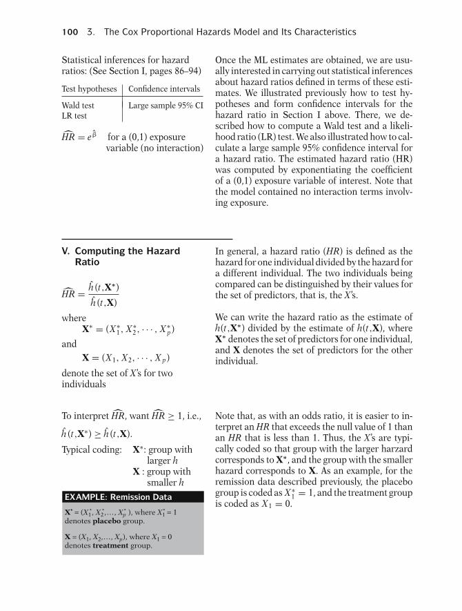
100 3. The Cox Proportional Hazards Model and Its Characteristics
Statistical inferences for hazardratios: (See Section I, pages 86–94)
Test hypotheses Confidence intervals
Wald test Large sample 95% CILR test
HR = eβ for a (0,1) exposurevariable (no interaction)
Once the ML estimates are obtained, we are usu-ally interested in carrying out statistical inferencesabout hazard ratios defined in terms of these esti-mates. We illustrated previously how to test hy-potheses and form confidence intervals for thehazard ratio in Section I above. There, we de-scribed how to compute a Wald test and a likeli-hood ratio (LR) test. We also illustrated how to cal-culate a large sample 95% confidence interval fora hazard ratio. The estimated hazard ratio (HR)was computed by exponentiating the coefficientof a (0,1) exposure variable of interest. Note thatthe model contained no interaction terms involv-ing exposure.
V. Computing the HazardRatio
In general, a hazard ratio (HR) is defined as thehazard for one individual divided by the hazard fora different individual. The two individuals beingcompared can be distinguished by their values forthe set of predictors, that is, the X ’s.HR = h (t,X∗)
h (t,X)
whereX∗ = (X ∗
1, X ∗2, · · · , X ∗
p)
andX = (X1, X2, · · · , X p)
denote the set of X ’s for twoindividuals
We can write the hazard ratio as the estimate ofh(t,X∗) divided by the estimate of h(t,X), whereX∗ denotes the set of predictors for one individual,and X denotes the set of predictors for the otherindividual.
To interpret HR, want HR ≥ 1, i.e.,
h (t,X∗) ≥ h (t,X).
Typical coding: X∗: group withlarger h
X : group withsmaller h
Note that, as with an odds ratio, it is easier to in-terpret an HR that exceeds the null value of 1 thanan HR that is less than 1. Thus, the X ’s are typi-cally coded so that group with the larger harzardcorresponds to X∗, and the group with the smallerhazard corresponds to X. As an example, for theremission data described previously, the placebogroup is coded as X ∗
1 = 1, and the treatment groupis coded as X1 = 0.
EXAMPLE: Remission Data
X* = (X1*, X2
*,..., Xp* ), where X1
* = 1denotes placebo group.
X = (X1, X2,..., Xp), where X1 = 0denotes treatment group.

Presentation: V. Computing the Hazard Ratio 101
HR = h (t,X∗)
h (t,X)= h 0(t) e
p∑i=1
βi X ∗i
h 0(t) e
p∑i=1
βi Xi
We now obtain an expression for the HR formulain terms of the regression coefficients by substi-tuting the Cox model formula into the numeratorand denominator of the hazard ratio expression.This substitution is shown here. Notice that theonly difference in the numerator and denomina-tor are the X ∗’s versus the X ’s. Notice also that thebaseline hazards will cancel out.
HR = h 0(t) e
p∑i=1
βi X ∗i
h 0(t) e
p∑i=1
βi Xi
= e
p∑i=1
βi (X ∗i −Xi )
Using algebra involving exponentials, the hazardratio formula simplifies to the exponential expres-sion shown here. Thus, the hazard ratio is com-puted by exponentiating the sum of each βi “hat”times the difference between X ∗
i and Xi .
HR = exp[ p∑
i=1βi (X ∗
i − Xi )] An alternative way to write this formula, using ex-
ponential notation, is shown here. We will nowillustrate the use of this general formula througha few examples.
EXAMPLE
X = (X1, X2,..., Xp) = (X1), where X1denotes (0,1) exposure status (p = 1)
X1* = 1, X1 = 0
HR = exp[β1(X1* – X1)]
= exp[β1(1 – 0)] = eβ1
ˆ
Model 1:
Coef. Std. Err. P > |z| Haz. Ratio
Rx 1.509 0.410 0.000 4.523
Suppose, for example, there is only one X variableof interest, X1, which denotes (0,1) exposurestatus, so that p = 1. Then, the hazard ratiocomparing exposed to unexposed persons isobtained by letting X ∗
1 = 1 and X1 = 0 in thehazard ratio formula. The estimated hazard ratiothen becomes e to the quantity β1 “hat” times 1minus 0, which simplifies to e to the β1 “hat.”
Recall the remission data printout for model 1,which contains only the Rx variable, again shownhere. Then the estimated hazard ratio is obtainedby exponentiating the coefficient 1.509, whichgives the value 4.523 shown in the HR column ofthe output.
EXAMPLE 2Model 2:
Coef. Std. Err. p > |z| Haz. Ratio
Rx 1.294 0.422 0.002 3.648
log WBC 1.604 0.329 0.000 4.975
+
X* = (1, log WBC), X = (0, log WBC)
HR for effect of Rx adjusted for log WBC:
As a second example, consider the output formodel 2, which contains two variables, the Rx vari-able and log WBC. Then to obtain the hazard ratiofor the effect of the Rx variable adjusted for the logWBC variable, we let the vectors X∗ and X be de-fined as X∗ = (1, log WBC) and X = (0, log WBC).Here we assume that log WBC is the same for X ∗and X though unspecified.

102 3. The Cox Proportional Hazards Model and Its Characteristics
EXAMPLE 2 (continued)
HR = exp[β1(X*1−X1) + β1 (X*
2 − X2)]^ ^
= exp[1.294(1−0)
= exp[1.294(1) + 1.604(0)]=
+ 1.604 (log WBC− log WBC)]
e1.294
ˆThe estimated hazard ratio is then obtained byexponentiating the sum of two quantities, oneinvolving the coefficient 1.294 of the Rx variable,and the other involving the coefficient 1.604 of thelog WBC variable. Since the log WBC value is fixed,however, this portion of the exponential is zero, sothat the resulting estimate is simply e to the 1.294.
General rule: If X1 is a (0,1)exposure variable, then
HR = eβ1 (= effect of exposureadjusted for other X ’s)
provided no other X ’s are productterms involving exposure.
This second example illustrates the general rulethat the hazard ratio for the effect of a (0,1) ex-posure variable which adjusts for other variablesis obtained by exponentiating the estimated coef-ficient of the exposure variable. This rule has theproviso that the model does not contain any prod-uct terms involving exposure.
EXAMPLE 3Model 3:
Coef. Std. Err. p > |z| Haz. Ratio
Rx 2.355 1.681 0.161 10.537
log WBC 1.803 0.447 0.000 6.067
Rx × log WBC −0.342 0.520 0.510 0.710
Want HR for effect of Rx adjusted forlog WBC.
Placebo subject: X* = (X1
* = 1, X2* = log WBC,
X3* = 1 × log WBC)
Treated subject: X = (X1 = 0, X2 = log WBC,
X3 = 0 × log WBC)
HR = exp[ˆ ∑3
βi(Xi* − Xi)]
HR = exp[2.355(1 − 0) + 1.803 (log WBC − log WBC) + (−0.342)(1 × log WBC
0 × log WBC)]
ˆi=1
= exp[2.355 − 0.342 log WBC]
−
We now give a third example which illustrateshow to compute a hazard ratio when the modeldoes contain product terms. We consider theprintout for model 3 of the remission data shownhere.
To obtain the hazard ratio for the effect of Rxadjusted for log WBC using model 3, we considerX ∗ and X vectors which have three components,one for each variable in the model. The X∗ vector,which denotes a placebo subject, has componentsX ∗
1 = 1, X ∗2 = log WBC and X ∗
3 = 1 times logWBC. The X vector, which denotes a treatedsubject, has components X1 = 0, X2 = log WBCand X3 = 0 times log WBC. Note again that, aswith the previous example, the value for log WBCis treated as fixed, though unspecified.
Using the general formula for the hazard ratio,we must now compute the exponential of the sumof three quantities, corresponding to the threevariables in the model. Substituting the valuesfrom the printout and the values of the vectors X∗and X into this formula, we obtain the exponen-tial expression shown here. Using algebra, thisexpression simplifies to the exponential of 2.355minus 0.342 times log WBC.

Presentation: VI. Adjusted Survival Curves Using the Cox PH Model 103
EXAMPLE 3 (continued)
log WBC = 2:
HR = exp[2.355 − 0.342 (2)] = e1.671 = 5.32
ˆlog WBC = 4:
HR = exp[2.355 − 0.342 (4)] = e0.987= 2.68
ˆ
In order to get a numerical value for the hazardratio, we must specify a value for log WBC. Forinstance, if log WBC = 2, the estimated hazardratio becomes 5.32, whereas if log WBC = 4, theestimated hazard ratio becomes 2.68. Thus, we getdifferent hazard ratio values for different values oflog WBC, which should make sense since log WBCis an effect modifier in model 3.
General rule for (0,1) exposurevariables when there are productterms:
HR = exp[β + ∑
δ j Wj
]where
β = coefficient of Eδ j = coefficient of E × Wj
(HR does not contain coefficientsof non-product terms)
The example we have just described using model3 illustrates a general rule which states that thehazard ratio for the effect of a (0,1) exposure vari-able in a model which contains product terms in-volving this exposure with other X ’s can be writtenas shown here. Note that β “hat” denotes the co-efficient of the exposure variable and the δ “hats”are coefficients of product terms in the model ofthe form ExWj . Also note that this formula doesnot contain coefficients of nonproduct terms otherthan those involving E.
EXAMPLE
Model 3:
HR (model 3) = exp[β + δ1 log WBC]= exp[2.355 – 0.342 log WBC]ˆ
β = coefficient of Rx
δ1= coefficient of Rx × log WBC
W1E
For model 3, β “hat” is the coefficient of the Rxvariable, and there is only one δ “hat” in thesum, which is the coefficient of the product termRx × log WBC. Thus, there is only one W, namelyW1 = log WBC. The hazard ratio formula for theeffect of exposure is then given by exponentiatingβ “hat” plus δ1 “hat” times log WBC. Substitutingthe estimates from the printout into this formulayields the expression obtained previously, namelythe exponential of 2.355 minus 0.342 times logWBC.
VI. Adjusted Survival CurvesUsing the Cox PH Model
Two primary quantities:
1. estimated hazard ratios2. estimated survival curves
The two primary quantities desired from a sur-vival analysis point of view are estimated hazardratios and estimated survival curves. Having justdescribed how to compute hazard ratios, we nowturn to estimation of survival curves using the Coxmodel.

104 3. The Cox Proportional Hazards Model and Its Characteristics
No model: use KM curves1.0
0.5
010 20t in weeks
Treatmentgroup
Placebogroup
S(t)
Recall that if no model is used to fit survival data,a survival curve can be estimated using a Kaplan–Meier method. Such KM curves are plotted as stepfunctions as shown here for the remission dataexample.
Cox model: adjusted survivalcurves (also step functions).
When a Cox model is used to fit survival data, sur-vival curves can be obtained that adjust for theexplanatory variables used as predictors. Theseare called adjusted survival curves, and, like KMcurves, these are also plotted as step functions.
Cox model hazard function:
h(t,X) = h0(t) e
p∑i=1
βi Xi
Cox model survival function:
S(t,X) = [S0(t)
]e
p∑i=1
βi Xi
The hazard function formula for the Cox PHmodel, shown here again, can be converted to acorresponding survival function formula as shownbelow. This survival function formula is the ba-sis for determining adjusted survival curves. Notethat this formula says that the survival function attime t for a subject with vector X as predictors isgiven by a baseline survival function S0(t) raisedto a power equal to the exponential of the sum ofβi times Xi .
Estimated survival function:
S(t,X) = [S0(t)
]e
p∑i=1
βi Xi
The expression for the estimated survival functioncan then be written with the usual “hat” notationas shown here.
S0(t) and βi are provided by thecomputer program. The Xi mustbe specified by the investigator.
The estimates of S0(t) and βi are provided by thecomputer program that fits the Cox model. TheX ’s, however, must first be specified by the investi-gator before the computer program can computethe estimated survival curve.

Presentation: VI. Adjusted Survival Curves Using the Cox PH Model 105
EXAMPLE: Model 2 Remission Data
h(t,X) = h0(t)e1.294 Rx + 1.604 log WBC
S(t,X) = [S0(t)]exp(1.294 Rx + 1.604 log WBC)
Rx = 0, log WBC = 2.93:
Specify values for X = (Rx, log WBC):
Rx = 1, log WBC = 2.93:
Adjusted Survival Curves
Rx = 1, log WBC = 2.93: S ˆ
ˆ ˆ
(t,X) = [S0(t)]400.9
Rx = 0, log WBC = 2.93: S(t,X) = [S0(t)]109.9
S(t,X) = [S0(t)]exp(1.294 (1) + 1.604 (2.93))
= [S0(t)]exp(5.99 ) = [S0(t)]400.9
S(t,X) = [S0(t)]exp(1.294 (0) + 1.604 (2.93))
= [S0(t)]exp(4.70) = [S0(t)]109.9
For example, if we consider model 2 for theremission data, the fitted model written in termsof both the hazard function and correspondingsurvival function is given here.
We can obtain a specific survival curve byspecifying values for the vector X, whose compo-nent variables are Rx and log WBC.
For instance, if Rx = 1 and log WBC = 2.93,the estimated survival curve is obtained bysubstituting these values in the formula as shownhere, and carrying out the algebra to obtain theexpression circled. Note that the value 2.93 is theoverall mean log WBC for the entire dataset of 42subjects.
Also, if Rx = 0 and log WBC = 2.93, the es-timated survival curve is obtained as shown here.
Each of the circled expressions gives ad-justed survival curves, where the adjustment isfor the values specified for the X ’s. Note that foreach expression, a survival probability can beobtained for any value of t.
The two formulae just obtained, again shownhere, allow us to compare survival curves for dif-ferent treatment groups adjusted for the covariatelog WBC. Both curves describe estimated survivalprobabilities over time assuming the same valueof log WBC, in this case, the value 2.93.
Typically, use X = X or Xmedian.
Computer uses X .
Typically, when computing adjusted survivalcurves, the value chosen for a covariate being ad-justed is an average value like an arithmetic meanor a median. In fact, most computer programs forthe Cox model automatically use the mean valueover all subjects for each covariate being adjusted.
EXAMPLE (continued)
Remission data (n = 42):
log WBC = 2.93
In our example, the mean log WBC for all 42 sub-jects in the remission data set is 2.93. That is whywe chose this value for log WBC in the formulaefor the adjusted survival curve.
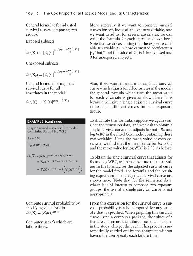
106 3. The Cox Proportional Hazards Model and Its Characteristics
General formulae for adjustedsurvival curves comparing twogroups:
Exposed subjects:
S(t,X1) = [S0(t)]exp[β1(1)+∑
i �=1βi X i ]
Unexposed subjects:
S(t,X0) = [S0(t)]exp[β1(0)+∑
i �=1βi X i ]
More generally, if we want to compare survivalcurves for two levels of an exposure variable, andwe want to adjust for several covariates, we canwrite the formula for each curve as shown here.Note that we are assuming that the exposure vari-able is variable X1, whose estimated coefficient isβ1 “hat,” and the value of X1 is 1 for exposed and0 for unexposed subjects.
General formula for adjustedsurvival curve for allcovariates in the model:
S(t, X) = [S0(t)]exp[∑
βi X i ]
Also, if we want to obtain an adjusted survivalcurve which adjusts for all covariates in the model,the general formula which uses the mean valuefor each covariate is given as shown here. Thisformula will give a single adjusted survival curverather than different curves for each exposuregroup.
EXAMPLE (continued)
Single survival curve for Cox modelcontaining Rx and log WBC:
Rx = 0.50
log WBC = 2.93
S(t,X) = [S0(t)]exp(
= [S0(t)]exp(1.294(0.5) + 1.604(2.93))
= [S0(t)]exp(5.35) = [S0(t)]210.6
β1Rx + β2log WBC)
To illustrate this formula, suppose we again con-sider the remission data, and we wish to obtain asingle survival curve that adjusts for both Rx andlog WBC in the fitted Cox model containing thesetwo variables. Using the mean value of each co-variate, we find that the mean value for Rx is 0.5and the mean value for log WBC is 2.93, as before.
To obtain the single survival curve that adjusts forRx and log WBC, we then substitute the mean val-ues in the formula for the adjusted survival curvefor the model fitted. The formula and the result-ing expression for the adjusted survival curve areshown here. (Note that for the remission data,where it is of interest to compare two exposuregroups, the use of a single survival curve is notappropriate.)
Compute survival probability byspecifying value for t inS(t,X) = [S0(t)]210.6
Computer uses t’s which arefailure times.
From this expression for the survival curve, a sur-vival probability can be computed for any valueof t that is specified. When graphing this survivalcurve using a computer package, the values of tthat are chosen are the failure times of all personsin the study who got the event. This process is au-tomatically carried out by the computer withouthaving the user specify each failure time.
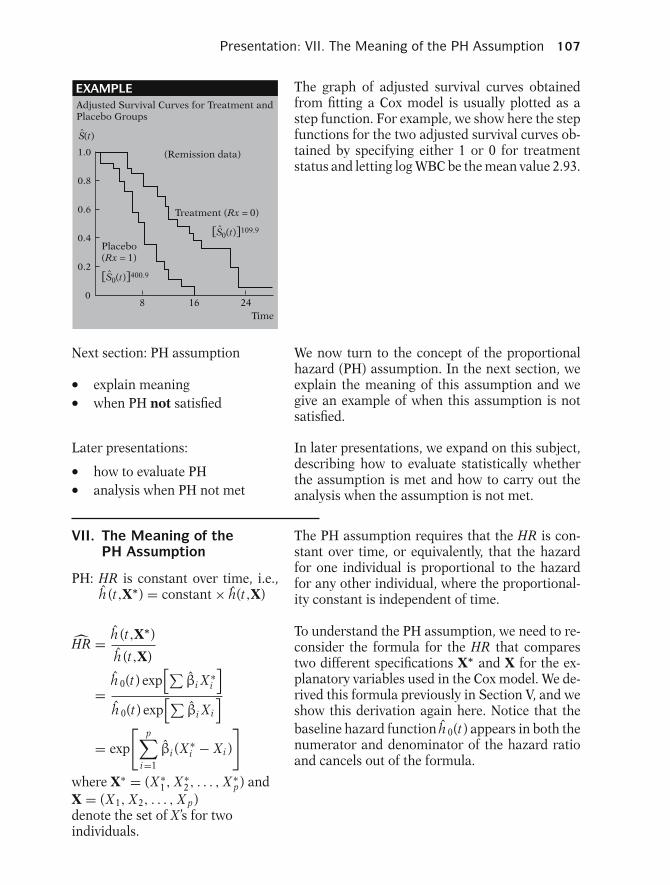
Presentation: VII. The Meaning of the PH Assumption 107
0.2
0
0.4
0.6
0.8
1.0
8 16 24
(Remission data)
Placebo(Rx = 1)
[S0(t)]400.9
Treatment (Rx = 0)
[S0(t)]109.9
Time
S(t)
EXAMPLEAdjusted Survival Curves for Treatment andPlacebo Groups
The graph of adjusted survival curves obtainedfrom fitting a Cox model is usually plotted as astep function. For example, we show here the stepfunctions for the two adjusted survival curves ob-tained by specifying either 1 or 0 for treatmentstatus and letting log WBC be the mean value 2.93.
Next section: PH assumption
� explain meaning� when PH not satisfied
We now turn to the concept of the proportionalhazard (PH) assumption. In the next section, weexplain the meaning of this assumption and wegive an example of when this assumption is notsatisfied.
Later presentations:� how to evaluate PH� analysis when PH not met
In later presentations, we expand on this subject,describing how to evaluate statistically whetherthe assumption is met and how to carry out theanalysis when the assumption is not met.
VII. The Meaning of thePH Assumption
PH: HR is constant over time, i.e.,h (t,X∗) = constant × h(t,X)
The PH assumption requires that the HR is con-stant over time, or equivalently, that the hazardfor one individual is proportional to the hazardfor any other individual, where the proportional-ity constant is independent of time.
HR = h (t,X∗)
h (t,X)
=h 0(t) exp
[∑βi X ∗
i
]h 0(t) exp
[∑βi Xi
]= exp
[p∑
i=1
βi (X ∗i − Xi )
]where X∗ = (X ∗
1, X ∗2, . . . , X ∗
p) andX = (X1, X2, . . . , X p)denote the set of X ’s for twoindividuals.
To understand the PH assumption, we need to re-consider the formula for the HR that comparestwo different specifications X∗ and X for the ex-planatory variables used in the Cox model. We de-rived this formula previously in Section V, and weshow this derivation again here. Notice that thebaseline hazard function h 0(t) appears in both thenumerator and denominator of the hazard ratioand cancels out of the formula.

108 3. The Cox Proportional Hazards Model and Its Characteristics
h (t,X∗)
h (t,X)= exp
[p∑
i=1
βi (X ∗i − Xi )
]does not involve t.
The final expression for the hazard ratio thereforeinvolves the estimated coefficients β1 “hat” andthe values of X∗ and X for each variable. However,because the baseline hazard has canceled out, thefinal expression does not involve time t.
LetConstant↙
θ = exp
[p∑
i=1
βi (X ∗i − Xi )
]then
h (t,X∗)
h (t,X)= θ
Thus, once the model is fitted and the values forX∗ and X are specified, the value of the exponen-tial expression for the estimated hazard ratio is aconstant, which does not depend on time. If wedenote this constant by θ “hat,” then we can writethe hazard ratio as shown here. This is a mathe-matical expression which states the proportionalhazards assumption.
h(t, X*) = θh(t, X)
HR (X* versus X)
t
Proportionality constant(not dependent on time)
Graphically, this expression says that the esti-mated hazard ratio comparing any two individ-uals plots as a constant over time.
Another way to write the proportional hazardsassumption mathematically expresses the hazardfunction for individual X∗ as θ “hat” times thehazard function for individual X, as shown here.This expression says that the hazard function forone individual is proportional to the hazard func-tion for another individual, where the proportion-ality constant is θ “hat,” which does not dependon time.
HR =
h(t, X) = h0(t) e1.294 Rx+1.604 log WBC
h(t, Rx=1, log WBC = 2.93)
h(t, Rx=0, log WBC = 2.93)
h(t, Rx = 1, log WBC = 2.93)
= 3.65h(t, Rx = 0, log WBC = 2.93)
= exp[1.294] = 3.65 Constant
Placebo
3.65 = proportionality constantTreatment
EXAMPLE: Remission Data To illustrate the proportional hazard assumption,we again consider the Cox model for the remissiondata involving the two variables Rx and log WBC.For this model, the estimated hazard ratio thatcompares placebo (Rx = 1) with treated (Rx = 0)subjects controlling for log WBC is given by e tothe 1.294, which is 3.65, a constant.
Thus, the hazard for placebo group (Rx = 1) is3.65 times the hazard for the treatment group(Rx = 0), and the value, 3.65, is the same re-gardless of time. In other words, using the abovemodel, the hazard for the placebo group is propor-tional to the hazard for the treatment group, andthe proportionality constant is 3.65.

Presentation: VII. The Meaning of the PH Assumption 109
Is the above Cox PH model appropriate?
Note:
Serioussurgery
⇒ High risk for death early
Hazards cross
E = 0 (surgery)
E = 0
E = 1
E = 1 (no surgery)
2 days:
5 days:
h(t,X)
t(days)3
h(t = 2, E = 1)
h(t = 2, E = 0)<1
h(t = 5, E = 1)
h(t = 5, E = 0)>1
but
EXAMPLE: PH Not Satisfied
Cancer patientsSurgery
Radiation withno surgery
E = 0 if surgery1 if no surgery
h(t,X) = h0(t)eβE
To further illustrate the concept of proportionalhazards, we now provide an example of a situationfor which the proportional hazards assumption isnot satisfied.
For our example, we consider a study in whichcancer patients are randomized to either surgeryor radiation therapy without surgery. Thus, wehave a (0,1) exposure variable denoting surgerystatus, with 0 if a patient receives surgery and 1if not. Suppose further that this exposure variableis the only variable of interest, so that a Cox PHmodel for the analysis of this data, as shown here,will contain only the one variable E, denotingexposure.
Now the question we consider here is whether theabove Cox model containing the variable E is anappropriate model to use for this situation. To an-swer this question we note that when a patientundergoes serious surgery, as when removing acancerous tumor, there is usually a high risk forcomplications from surgery or perhaps even deathearly in the recovery process, and once the patientgets past this early critical period, the benefits ofsurgery, if any, can then be observed.
Thus, in a study that compares surgery to nosurgery, we might expect to see hazard functionsfor each group that appear as shown here. No-tice that these two functions cross at about threedays, and that prior to three days the hazardfor the surgery group is higher than the hazardfor the no surgery group, whereas after three days,the hazard for the surgery group is lower than thehazard for the no surgery group.
Looking at the above graph more closely, we cansee that at 2 days, when t = 2, the hazard ratio ofnon-surgery (E = 1) to surgery (E = 0) patientsyields a value less than 1. In contrast, at t = 5 days,the hazard ratio of nonsurgery to surgery yields avalue greater than 1.
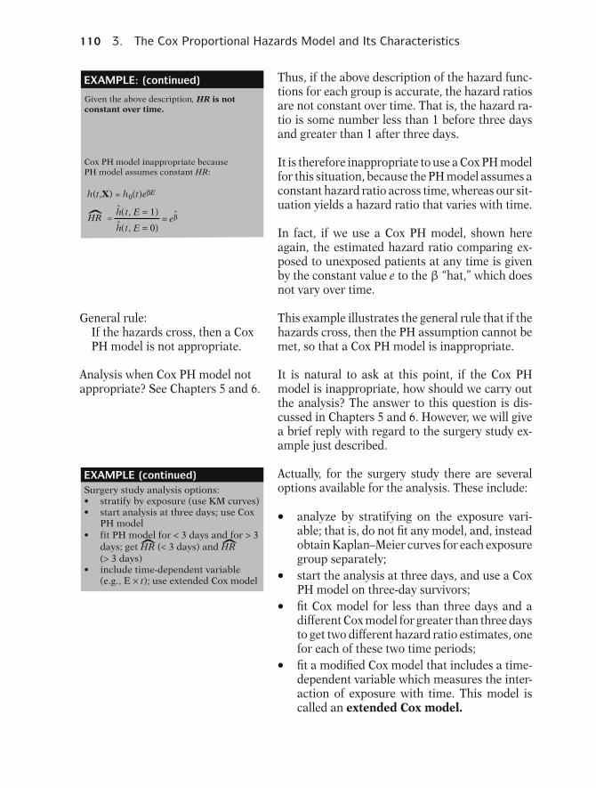
110 3. The Cox Proportional Hazards Model and Its Characteristics
EXAMPLE: (continued)
h(t, E = 1)
h(t, E = 0)
Given the above description, HR is notconstant over time.
Cox PH model inappropriate becausePH model assumes constant HR:
h(t,X) = h0(t)eβE
HR = = eβ
Thus, if the above description of the hazard func-tions for each group is accurate, the hazard ratiosare not constant over time. That is, the hazard ra-tio is some number less than 1 before three daysand greater than 1 after three days.
It is therefore inappropriate to use a Cox PH modelfor this situation, because the PH model assumes aconstant hazard ratio across time, whereas our sit-uation yields a hazard ratio that varies with time.
In fact, if we use a Cox PH model, shown hereagain, the estimated hazard ratio comparing ex-posed to unexposed patients at any time is givenby the constant value e to the β “hat,” which doesnot vary over time.
General rule:If the hazards cross, then a CoxPH model is not appropriate.
This example illustrates the general rule that if thehazards cross, then the PH assumption cannot bemet, so that a Cox PH model is inappropriate.
Analysis when Cox PH model notappropriate? See Chapters 5 and 6.
It is natural to ask at this point, if the Cox PHmodel is inappropriate, how should we carry outthe analysis? The answer to this question is dis-cussed in Chapters 5 and 6. However, we will givea brief reply with regard to the surgery study ex-ample just described.
EXAMPLE (continued) Surgery study analysis options: • stratify by exposure (use KM curves) • start analysis at three days; use Cox PH model • fit PH model for < 3 days and for > 3 days; get HR (< 3 days) and HR
(> 3 days) • include time-dependent variable
(e.g., E × t); use extended Cox model
ˆ ˆ
Actually, for the surgery study there are severaloptions available for the analysis. These include:
� analyze by stratifying on the exposure vari-able; that is, do not fit any model, and, insteadobtain Kaplan–Meier curves for each exposuregroup separately;� start the analysis at three days, and use a CoxPH model on three-day survivors;� fit Cox model for less than three days and adifferent Cox model for greater than three daysto get two different hazard ratio estimates, onefor each of these two time periods;� fit a modified Cox model that includes a time-dependent variable which measures the inter-action of exposure with time. This model iscalled an extended Cox model.
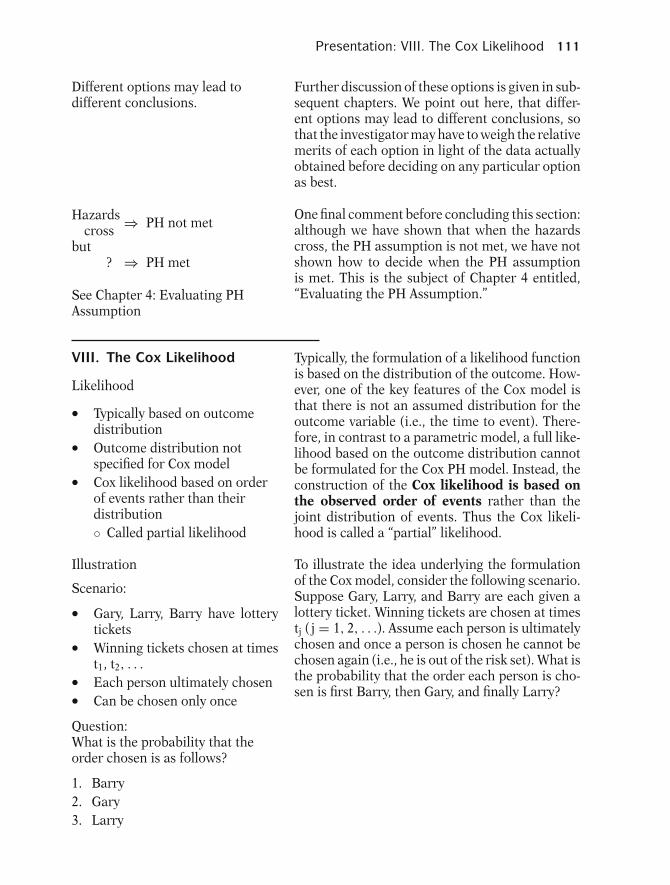
Presentation: VIII. The Cox Likelihood 111
Different options may lead todifferent conclusions.
Further discussion of these options is given in sub-sequent chapters. We point out here, that differ-ent options may lead to different conclusions, sothat the investigator may have to weigh the relativemerits of each option in light of the data actuallyobtained before deciding on any particular optionas best.
Hazards ⇒ PH not metcrossbut
? ⇒ PH met
See Chapter 4: Evaluating PHAssumption
One final comment before concluding this section:although we have shown that when the hazardscross, the PH assumption is not met, we have notshown how to decide when the PH assumptionis met. This is the subject of Chapter 4 entitled,“Evaluating the PH Assumption.”
VIII. The Cox Likelihood
Likelihood
� Typically based on outcomedistribution� Outcome distribution notspecified for Cox model� Cox likelihood based on orderof events rather than theirdistribution◦ Called partial likelihood
Typically, the formulation of a likelihood functionis based on the distribution of the outcome. How-ever, one of the key features of the Cox model isthat there is not an assumed distribution for theoutcome variable (i.e., the time to event). There-fore, in contrast to a parametric model, a full like-lihood based on the outcome distribution cannotbe formulated for the Cox PH model. Instead, theconstruction of the Cox likelihood is based onthe observed order of events rather than thejoint distribution of events. Thus the Cox likeli-hood is called a “partial” likelihood.
Illustration
Scenario:
� Gary, Larry, Barry have lotterytickets� Winning tickets chosen at timest1, t2, . . .� Each person ultimately chosen� Can be chosen only once
Question:What is the probability that theorder chosen is as follows?
1. Barry2. Gary3. Larry
To illustrate the idea underlying the formulationof the Cox model, consider the following scenario.Suppose Gary, Larry, and Barry are each given alottery ticket. Winning tickets are chosen at timestj ( j = 1, 2, . . .). Assume each person is ultimatelychosen and once a person is chosen he cannot bechosen again (i.e., he is out of the risk set). What isthe probability that the order each person is cho-sen is first Barry, then Gary, and finally Larry?
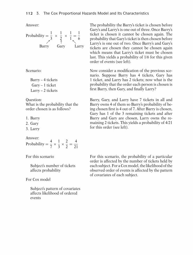
112 3. The Cox Proportional Hazards Model and Its Characteristics
Answer:
Probability = 13
× 12
× 11
= 16↗ ↑ ↖
Barry Gary Larry
The probability the Barry’s ticket is chosen beforeGary’s and Larry’s is one out of three. Once Barry’sticket is chosen it cannot be chosen again. Theprobability that Gary’s ticket is then chosen beforeLarry’s is one out of two. Once Barry’s and Gary’stickets are chosen they cannot be chosen againwhich means that Larry’s ticket must be chosenlast. This yields a probability of 1/6 for this givenorder of events (see left).
Scenario:
Barry – 4 ticketsGary – 1 ticket
Larry – 2 tickets
Now consider a modification of the previous sce-nario. Suppose Barry has 4 tickets, Gary has1 ticket, and Larry has 2 tickets; now what is theprobability that the order each person is chosen isfirst Barry, then Gary, and finally Larry?
Question:What is the probability that theorder chosen is as follows?
1. Barry2. Gary3. Larry
Answer:
Probability = 47
× 13
× 22
= 421
Barry, Gary, and Larry have 7 tickets in all andBarry owns 4 of them so Barry’s probability of be-ing chosen first is 4 out of 7. After Barry is chosen,Gary has 1 of the 3 remaining tickets and afterBarry and Gary are chosen, Larry owns the re-maining 2 tickets. This yields a probability of 4/21for this order (see left).
For this scenario
Subject’s number of ticketsaffects probability
For Cox model
Subject’s pattern of covariatesaffects likelihood of orderedevents
For this scenario, the probability of a particularorder is affected by the number of tickets held byeach subject. For a Cox model, the likelihood of theobserved order of events is affected by the patternof covariates of each subject.
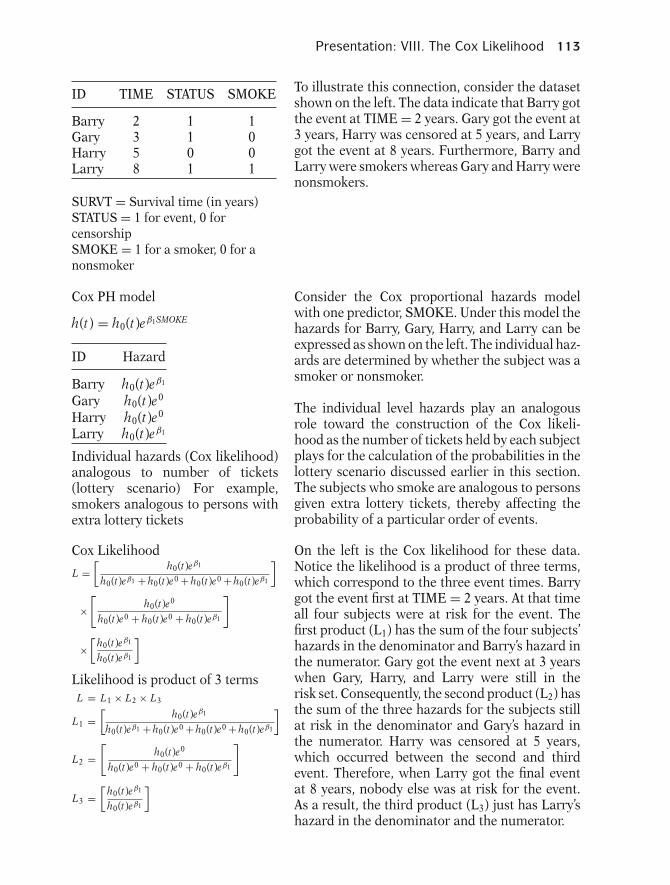
Presentation: VIII. The Cox Likelihood 113
ID TIME STATUS SMOKE
Barry 2 1 1Gary 3 1 0Harry 5 0 0Larry 8 1 1
SURVT = Survival time (in years)STATUS = 1 for event, 0 forcensorshipSMOKE = 1 for a smoker, 0 for anonsmoker
To illustrate this connection, consider the datasetshown on the left. The data indicate that Barry gotthe event at TIME = 2 years. Gary got the event at3 years, Harry was censored at 5 years, and Larrygot the event at 8 years. Furthermore, Barry andLarry were smokers whereas Gary and Harry werenonsmokers.
Cox PH model
h(t) = h0(t)eβ1SMOKE
ID Hazard
Barry h0(t)eβ1
Gary h0(t)e0
Harry h0(t)e0
Larry h0(t)eβ1
Individual hazards (Cox likelihood)analogous to number of tickets(lottery scenario) For example,smokers analogous to persons withextra lottery tickets
Consider the Cox proportional hazards modelwith one predictor, SMOKE. Under this model thehazards for Barry, Gary, Harry, and Larry can beexpressed as shown on the left. The individual haz-ards are determined by whether the subject was asmoker or nonsmoker.
The individual level hazards play an analogousrole toward the construction of the Cox likeli-hood as the number of tickets held by each subjectplays for the calculation of the probabilities in thelottery scenario discussed earlier in this section.The subjects who smoke are analogous to personsgiven extra lottery tickets, thereby affecting theprobability of a particular order of events.
Cox Likelihood
L =[
h0(t)eβ1
h0(t)eβ1 + h0(t)e0 + h0(t)e0 + h0(t)eβ1
]
×[
h0(t)e0
h0(t)e0 + h0(t)e0 + h0(t)eβ1
]
×[
h0(t)eβ1
h0(t)eβ1
]Likelihood is product of 3 termsL = L1 × L2 × L3
L1 =[
h0(t)eβ1
h0(t)eβ1 + h0(t)e0 + h0(t)e0 + h0(t)eβ1
]
L2 =[
h0(t)e0
h0(t)e0 + h0(t)e0 + h0(t)eβ1
]
L3 =[
h0(t)eβ1
h0(t)eβ1
]
On the left is the Cox likelihood for these data.Notice the likelihood is a product of three terms,which correspond to the three event times. Barrygot the event first at TIME = 2 years. At that timeall four subjects were at risk for the event. Thefirst product (L1) has the sum of the four subjects’hazards in the denominator and Barry’s hazard inthe numerator. Gary got the event next at 3 yearswhen Gary, Harry, and Larry were still in therisk set. Consequently, the second product (L2) hasthe sum of the three hazards for the subjects stillat risk in the denominator and Gary’s hazard inthe numerator. Harry was censored at 5 years,which occurred between the second and thirdevent. Therefore, when Larry got the final eventat 8 years, nobody else was at risk for the event.As a result, the third product (L3) just has Larry’shazard in the denominator and the numerator.

114 3. The Cox Proportional Hazards Model and Its Characteristics
t1, time = 2, four at risk (L1)t2, time = 3, three at risk (L2)t3, time = 8, one at risk (L3)
For each term:
Numerator—single hazardDenominator—sum of hazards
To summarize, the likelihood in our example con-sists of a product of three terms (L1, L2, and L3)corresponding to the ordered failure times (t1, t2,and t3). The denominator for the term correspond-ing to time tj ( j = 1, 2, 3) is the sum of the hazardsfor those subjects still at risk at time tj, and thenumerator is the hazard for the subject who gotthe event at tj.
Baseline hazard, h0(t) cancels
L =[
eβ1
eβ1 + e0 + e0 + eβ1
]×
[e0
e0 + e0 + eβ1
]×
[eβ1
eβ1
]Thus, L does not depend on h0(t)
A key property of the Cox likelihood is that thebaseline hazard cancels out in each term. Thus,the form of the baseline hazard need not be spec-ified in a Cox model, as it plays no role in the esti-mation of the regression parameters. By factoringh0(t) in the denominator and then canceling it outof each term, the likelihood for Barry, Gary, andLarry can be rewritten as shown on the left.
Data A
ID TIME STATUS SMOKE
Barry 2 1 1Gary 3 1 0Harry 5 0 0Larry 8 1 1
Data B
ID TIME STATUS SMOKE
Barry 1 1 1Gary 7 1 0Harry 8 0 0Larry 63 1 1
Comparing datasets
� TIME variable differs� Order of events the same� Cox PH likelihood the same
As we mentioned earlier, the Cox likelihood is de-termined by the order of events and censorshipsand not by the distribution of the outcome vari-able. To illustrate this point, compare datasetsA and B on the left, and consider the likelihoodfor a Cox PH model with smoking status as theonly predictor. Although the values for the variableTIME differ in the two datasets, the Cox likelihoodwill be the same using either dataset because theorder of the outcome (TIME) remains unchanged.
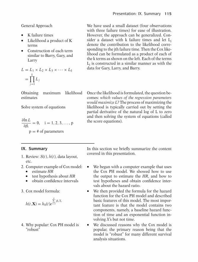
Presentation: IX. Summary 115
General Approach
� K failure times� Likelihood a product of Kterms� Construction of each termsimilar to Barry, Gary, andLarry
L = L1 × L2 × L3 × · · · × Lk
=k∏
j=1
L j
We have used a small dataset (four observationswith three failure times) for ease of illustration.However, the approach can be generalized. Con-sider a dataset with k failure times and let Ljdenote the contribution to the likelihood corre-sponding to the jth failure time. Then the Cox like-lihood can be formulated as a product of each ofthe k terms as shown on the left. Each of the termsLj is constructed in a similar manner as with thedata for Gary, Larry, and Barry.
Obtaining maximum likelihoodestimates
Solve system of equations
∂ ln L∂βi
= 0, i = 1, 2, 3, . . . , p
p = # of parameters
Once the likelihood is formulated, the question be-comes: which values of the regression parameterswould maximize L? The process of maximizing thelikelihood is typically carried out by setting thepartial derivative of the natural log of L to zeroand then solving the system of equations (calledthe score equations).
IX. Summary
1. Review: S(t), h(t), data layout,etc.
In this section we briefly summarize the contentcovered in this presentation.
2. Computer example of Cox model:� estimate HR� test hypothesis about HR� obtain confidence intervals
3. Cox model formula:
h(t,X) = h0(t)e
p∑i=1
βi Xi
� We began with a computer example that usesthe Cox PH model. We showed how to usethe output to estimate the HR, and how totest hypotheses and obtain confidence inter-vals about the hazard ratio.� We then provided the formula for the hazardfunction for the Cox PH model and describedbasic features of this model. The most impor-tant feature is that the model contains twocomponents, namely, a baseline hazard func-tion of time and an exponential function in-volving X ’s but not time.
4. Why popular: Cox PH model is“robust”
� We discussed reasons why the Cox model ispopular, the primary reason being that themodel is “robust” for many different survivalanalysis situations.
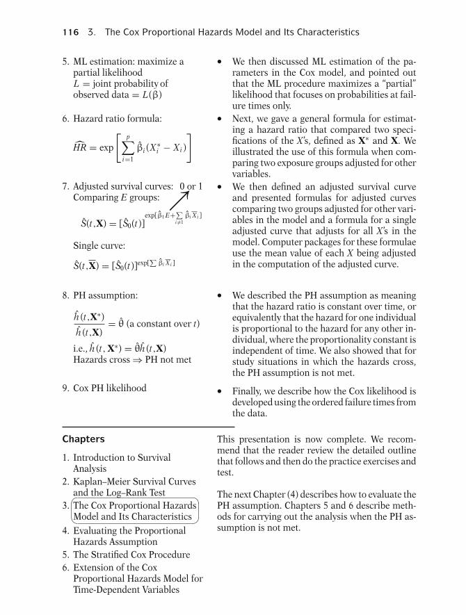
116 3. The Cox Proportional Hazards Model and Its Characteristics
5. ML estimation: maximize apartial likelihoodL = joint probability ofobserved data = L(β)
6. Hazard ratio formula:
HR = exp
[p∑
i=1
βi (X ∗i − Xi )
]
7. Adjusted survival curves: 0 or 1Comparing E groups: ↗
S(t,X) = [S0(t)]exp[β1 E+∑
i �=1βi X i ]
Single curve:
S(t,X) = [S0(t)]exp[∑
βi X i ]
8. PH assumption:
h (t,X∗)
h (t,X)= θ (a constant over t)
i.e., h (t, X∗) = θh (t,X)Hazards cross ⇒ PH not met
9. Cox PH likelihood
� We then discussed ML estimation of the pa-rameters in the Cox model, and pointed outthat the ML procedure maximizes a “partial”likelihood that focuses on probabilities at fail-ure times only.� Next, we gave a general formula for estimat-ing a hazard ratio that compared two speci-fications of the X ’s, defined as X∗ and X. Weillustrated the use of this formula when com-paring two exposure groups adjusted for othervariables.� We then defined an adjusted survival curveand presented formulas for adjusted curvescomparing two groups adjusted for other vari-ables in the model and a formula for a singleadjusted curve that adjusts for all X ’s in themodel. Computer packages for these formulaeuse the mean value of each X being adjustedin the computation of the adjusted curve.
� We described the PH assumption as meaningthat the hazard ratio is constant over time, orequivalently that the hazard for one individualis proportional to the hazard for any other in-dividual, where the proportionality constant isindependent of time. We also showed that forstudy situations in which the hazards cross,the PH assumption is not met.
� Finally, we describe how the Cox likelihood isdeveloped using the ordered failure times fromthe data.
Chapters
1. Introduction to SurvivalAnalysis
2. Kaplan–Meier Survival Curvesand the Log–Rank Test
3. The Cox Proportional HazardsModel and Its Characteristics
�
�
�
�4. Evaluating the Proportional
Hazards Assumption5. The Stratified Cox Procedure6. Extension of the Cox
Proportional Hazards Model forTime-Dependent Variables
This presentation is now complete. We recom-mend that the reader review the detailed outlinethat follows and then do the practice exercises andtest.
The next Chapter (4) describes how to evaluate thePH assumption. Chapters 5 and 6 describe meth-ods for carrying out the analysis when the PH as-sumption is not met.
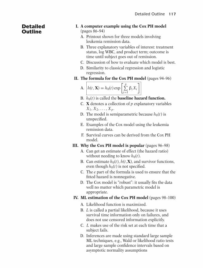
Detailed Outline 117
DetailedOutline
I. A computer example using the Cox PH model(pages 86–94)A. Printout shown for three models involving
leukemia remission data.B. Three explanatory variables of interest: treatment
status, log WBC, and product term; outcome istime until subject goes out of remission.
C. Discussion of how to evaluate which model is best.D. Similarity to classical regression and logistic
regression.II. The formula for the Cox PH model (pages 94–96)
A. h(t, X) = h0(t) exp[ p∑
i=1βi Xi
]B. h0(t) is called the baseline hazard function.C. X denotes a collection of p explanatory variables
X1, X2, . . . , X p.D. The model is semiparametric because h0(t) is
unspecified.E. Examples of the Cox model using the leukemia
remission data.F. Survival curves can be derived from the Cox PH
model.III. Why the Cox PH model is popular (pages 96–98)
A. Can get an estimate of effect (the hazard ratio)without needing to know h0(t).
B. Can estimate h0(t), h(t,X), and survivor functions,even though h0(t) is not specified.
C. The e part of the formula is used to ensure that thefitted hazard is nonnegative.
D. The Cox model is “robust”: it usually fits the datawell no matter which parametric model isappropriate.
IV. ML estimation of the Cox PH model (pages 98–100)
A. Likelihood function is maximized.B. L is called a partial likelihood, because it uses
survival time information only on failures, anddoes not use censored information explicitly.
C. L makes use of the risk set at each time that asubject fails.
D. Inferences are made using standard large sampleML techniques, e.g., Wald or likelihood ratio testsand large sample confidence intervals based onasymptotic normality assumptions

118 3. The Cox Proportional Hazards Model and Its Characteristics
V. Computing the hazard ratio (pages 100–103)A. Formula for hazard ratio comparing two
individuals, X∗ = (X ∗1, X ∗
2, . . . , X ∗p) and
X = (X1, X2, . . . , X p):
h(t, X∗)h(t,X)
= exp
[p∑
i=1
βi (X ∗i − Xi )
]B. Examples are given using a (0,1) exposure variable,
potential confounders, and potential effectmodifiers.
C. Typical coding identifies X∗ as the group with thelarger hazard and X as the group with the smallerhazard, e.g., X ∗
1 = 1 for unexposed group andX1 = 0 for exposed group.
VI. Adjusted survival curves using the Cox PH model(pages 103–107)A. Survival curve formula can be obtained from
hazard ratio formula:
S(t, X) = [S0(t)]exp[∑
βi Xi ]
where S0(t) is the baseline survival function thatcorresponds to the baseline hazard function h0(t).
B. To graph S(t,X), must specify values forX = (X1, X2, . . . , X p).
C. To obtain “adjusted” survival curves, usually useoverall mean values for the X ’s being adjusted.
D. Examples of “adjusted” S(t, X) using leukemiaremission data.
VII. The meaning of the PH assumption (pages 107–111)A. Hazard ratio formula shows that hazard ratio is
independent of time:
h(t, X∗)h(t, X)
= θ
B. Baseline hazard function not involved in the HRformula.
C. Hazard ratio for two X’s are proportional:h(t, X∗) = θ h(t, X)
D. An example when the PH assumption is notsatisfied: hazards cross
VIII. Cox likelihood (pages 111–115)A. Lottery ExampleB. Likelihood based on order of events
IX. Summary (pages 115–116)
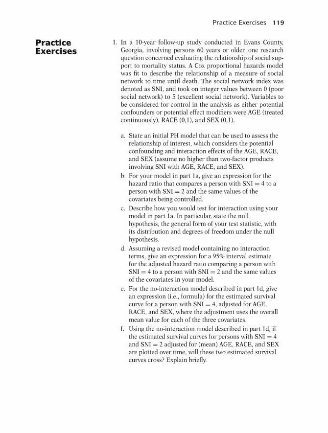
Practice Exercises 119
PracticeExercises
1. In a 10-year follow-up study conducted in Evans County,Georgia, involving persons 60 years or older, one researchquestion concerned evaluating the relationship of social sup-port to mortality status. A Cox proportional hazards modelwas fit to describe the relationship of a measure of socialnetwork to time until death. The social network index wasdenoted as SNI, and took on integer values between 0 (poorsocial network) to 5 (excellent social network). Variables tobe considered for control in the analysis as either potentialconfounders or potential effect modifiers were AGE (treatedcontinuously), RACE (0,1), and SEX (0,1).
a. State an initial PH model that can be used to assess therelationship of interest, which considers the potentialconfounding and interaction effects of the AGE, RACE,and SEX (assume no higher than two-factor productsinvolving SNI with AGE, RACE, and SEX).
b. For your model in part 1a, give an expression for thehazard ratio that compares a person with SNI = 4 to aperson with SNI = 2 and the same values of thecovariates being controlled.
c. Describe how you would test for interaction using yourmodel in part 1a. In particular, state the nullhypothesis, the general form of your test statistic, withits distribution and degrees of freedom under the nullhypothesis.
d. Assuming a revised model containing no interactionterms, give an expression for a 95% interval estimatefor the adjusted hazard ratio comparing a person withSNI = 4 to a person with SNI = 2 and the same valuesof the covariates in your model.
e. For the no-interaction model described in part 1d, givean expression (i.e., formula) for the estimated survivalcurve for a person with SNI = 4, adjusted for AGE,RACE, and SEX, where the adjustment uses the overallmean value for each of the three covariates.
f. Using the no-interaction model described in part 1d, ifthe estimated survival curves for persons with SNI = 4and SNI = 2 adjusted for (mean) AGE, RACE, and SEXare plotted over time, will these two estimated survivalcurves cross? Explain briefly.
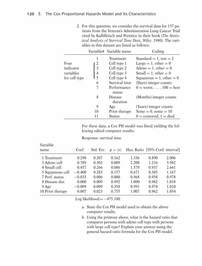
120 3. The Cox Proportional Hazards Model and Its Characteristics
2. For this question, we consider the survival data for 137 pa-tients from the Veteran’s Administration Lung Cancer Trialcited by Kalbfleisch and Prentice in their book (The Statis-tical Analysis of Survival Time Data, Wiley, 1980). The vari-ables in this dataset are listed as follows:
Variable# Variable name Coding
1 Treatment Standard = 1, test = 2Four 2 Cell type 1 Large = 1, other = 0indicator 3 Cell type 2 Adeno = 1, other = 0
⎧⎪⎨⎪⎩variables 4 Cell type 3 Small = 1, other = 0for cell type 5 Cell type 4 Squamous = 1, other = 0
6 Survival time (Days) integer counts7 Performance 0 = worst, . . . , 100 = best
status8 Disease (Months) integer counts
duration9 Age (Years) integer counts
10 Prior therapy None = 0, some = 1011 Status 0 = censored, 1 = died
For these data, a Cox PH model was fitted yielding the fol-lowing edited computer results:
Response: survival time
Variablename Coef. Std. Err. p > |z| Haz. Ratio [95% Conf. interval]
1 Treatment 0.290 0.207 0.162 1.336 0.890 2.0063 Adeno cell 0.789 0.303 0.009 2.200 1.216 3.9824 Small cell 0.457 0.266 0.086 1.579 0.937 2.6615 Squamous cell −0.400 0.283 0.157 0.671 0.385 1.1677 Perf. status −0.033 0.006 0.000 0.968 0.958 0.9788 Disease dur. 0.000 0.009 0.992 1.000 0.982 1.0189 Age −0.009 0.009 0.358 0.991 0.974 1.010
10 Prior therapy 0.007 0.023 0.755 1.007 0.962 1.054
Log likelihood = −475.180
a. State the Cox PH model used to obtain the abovecomputer results.
b. Using the printout above, what is the hazard ratio thatcompares persons with adeno cell type with personswith large cell type? Explain your answer using thegeneral hazard ratio formula for the Cox PH model.
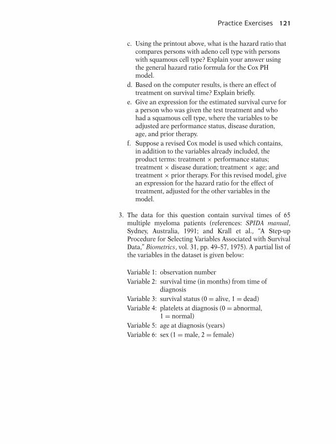
Practice Exercises 121
c. Using the printout above, what is the hazard ratio thatcompares persons with adeno cell type with personswith squamous cell type? Explain your answer usingthe general hazard ratio formula for the Cox PHmodel.
d. Based on the computer results, is there an effect oftreatment on survival time? Explain briefly.
e. Give an expression for the estimated survival curve fora person who was given the test treatment and whohad a squamous cell type, where the variables to beadjusted are performance status, disease duration,age, and prior therapy.
f. Suppose a revised Cox model is used which contains,in addition to the variables already included, theproduct terms: treatment × performance status;treatment × disease duration; treatment × age; andtreatment × prior therapy. For this revised model, givean expression for the hazard ratio for the effect oftreatment, adjusted for the other variables in themodel.
3. The data for this question contain survival times of 65multiple myeloma patients (references: SPIDA manual,Sydney, Australia, 1991; and Krall et al., “A Step-upProcedure for Selecting Variables Associated with SurvivalData,” Biometrics, vol. 31, pp. 49–57, 1975). A partial list ofthe variables in the dataset is given below:
Variable 1: observation numberVariable 2: survival time (in months) from time of
diagnosisVariable 3: survival status (0 = alive, 1 = dead)Variable 4: platelets at diagnosis (0 = abnormal,
1 = normal)Variable 5: age at diagnosis (years)Variable 6: sex (1 = male, 2 = female)

122 3. The Cox Proportional Hazards Model and Its Characteristics
Below, we provide edited computer results for severaldifferent Cox models that were fit to this dataset. A numberof questions will be asked about these results.
Model 1:Variable Coef. Std. Err. p > |z| Haz. Ratio [95% Conf. Interval]
Platelets 0.470 2.854 .869 1.600 0.006 429.689Age 0.000 0.037 .998 1.000 0.930 1.075Sex 0.183 0.725 .801 1.200 0.290 4.969Platelets × age −0.008 0.041 .850 0.992 0.915 1.075Platelets × sex −0.503 0.804 .532 0.605 0.125 2.924
Log likelihood = −153.040Model 2:Platelets −0.725 0.401 .071 0.484 0.221 1.063Age −0.005 0.016 .740 0.995 0.965 1.026Sex −0.221 0.311 .478 0.802 0.436 1.476
Log likelihood = −153.253Model 3:Platelets −0.706 0.401 .078 0.493 0.225 1.083Age −0.003 0.015 .828 0.997 0.967 1.027
Log likelihood = −153.509Model 4:Platelets −0.705 0.397 .076 0.494 0.227 1.075Sex −0.204 0.307 .506 0.815 0.447 1.489
Log likelihood = −153.308Model 5:Platelets −0.694 0.397 .080 0.500 0.230 1.088
Log likelihood = −153.533a. For model 1, give an expression for the hazard ratio
for the effect of the platelet variable adjusted for ageand sex.
b. Using your answer to part 3a, compute the estimatedhazard ratio for a 40-year-old male. Also compute theestimated hazard ratio for a 50-year-old female.
c. Carry out an appropriate test of hypothesis to evaluatewhether there is any significant interaction in model 1.What is your conclusion?
d. Considering models 2–5, evaluate whether age and sexneed to be controlled as confounders?
e. Which of the five models do you think is the bestmodel and why?
f. Based on your answer to part 3e, summarize theresults that describe the effect of the platelet variableon survival adjusted for age and sex.
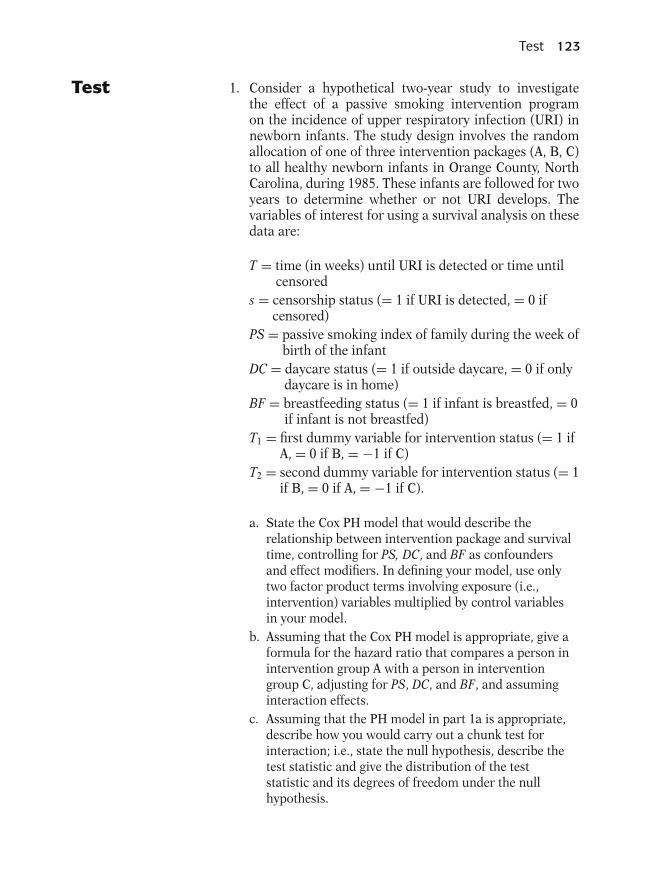
Test 123
Test 1. Consider a hypothetical two-year study to investigatethe effect of a passive smoking intervention programon the incidence of upper respiratory infection (URI) innewborn infants. The study design involves the randomallocation of one of three intervention packages (A, B, C)to all healthy newborn infants in Orange County, NorthCarolina, during 1985. These infants are followed for twoyears to determine whether or not URI develops. Thevariables of interest for using a survival analysis on thesedata are:
T = time (in weeks) until URI is detected or time untilcensored
s = censorship status (= 1 if URI is detected, = 0 ifcensored)
PS = passive smoking index of family during the week ofbirth of the infant
DC = daycare status (= 1 if outside daycare, = 0 if onlydaycare is in home)
BF = breastfeeding status (= 1 if infant is breastfed, = 0if infant is not breastfed)
T1 = first dummy variable for intervention status (= 1 ifA, = 0 if B, = −1 if C)
T2 = second dummy variable for intervention status (= 1if B, = 0 if A, = −1 if C).
a. State the Cox PH model that would describe therelationship between intervention package and survivaltime, controlling for PS, DC, and BF as confoundersand effect modifiers. In defining your model, use onlytwo factor product terms involving exposure (i.e.,intervention) variables multiplied by control variablesin your model.
b. Assuming that the Cox PH model is appropriate, give aformula for the hazard ratio that compares a person inintervention group A with a person in interventiongroup C, adjusting for PS, DC, and BF, and assuminginteraction effects.
c. Assuming that the PH model in part 1a is appropriate,describe how you would carry out a chunk test forinteraction; i.e., state the null hypothesis, describe thetest statistic and give the distribution of the teststatistic and its degrees of freedom under the nullhypothesis.

124 3. The Cox Proportional Hazards Model and Its Characteristics
d. Assuming no interaction effects, how would you testwhether packages A, B, and C are equally effective,after controlling for PS, DC, and BF in a Cox PH modelwithout interaction terms (i.e., state the two modelsbeing compared, the null hypothesis, the test statistic,and the distribution of the test statistic under the nullhypothesis).
e. For the no-interaction model considered in parts 1cand 1d, give an expression for the estimated survivalcurves for the effect of intervention A adjusted for PS,DC, and BF. Also, give similar (but different)expressions for the adjusted survival curves forinterventions B and C.
2. The data for this question consists of a sample of 50 per-sons from the 1967–1980 Evans County Study. There aretwo basic independent variables of interest: AGE andchronic disease status (CHR), where CHR is coded as0 = none, 1 = chronic disease. A product term of the formAGE × CHR is also considered. The dependent variableis time until death, and the event is death. The primaryquestion of interest concerns whether CHR, consideredas the exposure variable, is related to survival time, con-trolling for AGE. The edited output of computer resultsfor this question is given as follows:
Model 1:Variable Coef. Std. Err. Chi-sq p > |z|CHR 0.8595 0.3116 7.61 .0058
Log likelihood = −142.87
Model 2:CHR 0.8051 0.3252 6.13 .0133AGE 0.0856 0.0193 19.63 .0000
Log likelihood = −132.45
Model 3:CHR 1.0009 2.2556 0.20 .6572AGE 0.0874 0.0276 10.01 .0016CHR × AGE −0.0030 0.0345 0.01 .9301
Log likelihood = −132.35

Test 125
a. State the Cox PH model that allows for main effects ofCHR and AGE as well as the interaction effect of CHRwith AGE.
b. Carry out the test for significant interaction; i.e., statethe null hypothesis, the test statistic, and itsdistribution under the null hypothesis. What are yourconclusions about interaction?
c. Assuming no interaction, should AGE be controlled?Explain your answer on the basis of confoundingand/or precision considerations.
d. If, when considering plots of various hazard functionsover time, the hazard function for persons withCHR = 1 crosses the hazard function for persons withCHR = 0, what does this indicate about the use of anyof the three models provided in the printout?
e. Using model 2, give an expression for the estimatedsurvival curve for persons with CHR = 1, adjusted forAGE. Also, give an expression for the estimated survivalcurve for persons with CHR = 0, adjusted for AGE.
f. What is your overall conclusion about the effect ofCHR on survival time based on the computer resultsprovided from this study?
3. The data for this question contain remission times of42 multiple leukemia patients in a clinical trial of a newtreatment. The variables in the dataset are given below:
Variable 1: survival time (in weeks)Variable 2: status (1 = in remission, 0 = relapse)Variable 3: sex (1 = female, 0 = male)Variable 4: log WBCVariable 5: Rx status (1 = placebo, 0 = treatment)

126 3. The Cox Proportional Hazards Model and Its Characteristics
Below, we provide computer results for several differentCox models that were fit to this dataset. A number of ques-tions will be asked about these results starting below.
Model 1:Variable Coef. Std. Err. p > |z| Haz. Ratio [95% Conf.Interval]
Rx 0.894 1.815 .622 2.446 0.070 85.812Sex −1.012 0.752 .178 0.363 0.083 1.585log WBC 1.693 0.441 .000 5.437 2.292 12.897Rx × Sex 1.952 0.907 .031 7.046 1.191 41.702Rx × log WBC −0.151 0.531 .776 0.860 0.304 2.433
Log likelihood = −69.515Model 2:Rx 0.405 0.561 .470 1.500 0.499 4.507Sex −1.070 0.725 .140 0.343 0.083 1.422log WBC 1.610 0.332 .000 5.004 2.610 9.592Rx × Sex 2.013 0.883 .023 7.483 1.325 42.261
Log likelihood = −69.555Model 3:Rx 0.587 0.542 .279 1.798 0.621 5.202Sex −1.073 0.701 .126 0.342 0.087 1.353Rx × Sex 1.906 0.815 .019 6.726 1.362 33.213
Log likelihood = −83.475Model 4:Rx 1.391 0.457 .002 4.018 1.642 9.834Sex 0.263 0.449 .558 1.301 0.539 3.139log WBC 1.594 0.330 .000 4.922 2.578 9.397
Log likelihood = −72.109
a. Use the above computer results to carry out a chunktest to evaluate whether the two interaction terms inmodel 1 are significant. What are your conclusions?
b. Evaluate whether you would prefer model 1 ormodel 2. Explain your answer.
c. Using model 2, give an expression for the hazard ratiofor the effect of the Rx variable adjusted for SEX andlog WBC.
d. Using your answer in part 3c, compute the hazard ratiofor the effect of Rx for males and for females separately.
e. By considering the potential confounding of log WBC,determine which of models 2 and 3 you prefer. Explain.
f. Of the models provided which model do you considerto be best? Explain.
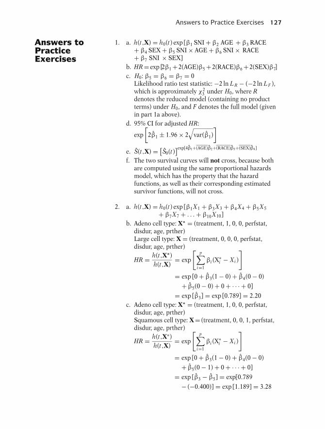
Answers to Practice Exercises 127
Answers toPracticeExercises
1. a. h(t,X) = h0(t) exp [β1 SNI + β2 AGE + β3 RACE+ β4 SEX + β5 SNI × AGE + β6 SNI × RACE+ β7 SNI × SEX]
b. HR = exp [2β1 +2(AGE)β5 +2(RACE)β6 +2(SEX)β7]c. H0: β5 = β6 = β7 = 0
Likelihood ratio test statistic: −2 ln L R − (−2 ln L F ),which is approximately χ2
3 under H0, where Rdenotes the reduced model (containing no productterms) under H0, and F denotes the full model (givenin part 1a above).
d. 95% CI for adjusted HR:
exp[
2β1 ± 1.96 × 2√
var(β1)]
e. S(t,X) = [S0(t)
]exp[4β1+(AGE)β2+(RACE)β3+(SEX)β4]
f. The two survival curves will not cross, because bothare computed using the same proportional hazardsmodel, which has the property that the hazardfunctions, as well as their corresponding estimatedsurvivor functions, will not cross.
2. a. h(t,X) = h0(t) exp [β1 X1 + β3 X3 + β4 X4 + β5 X5
+ β7 X7 + . . . + β10 X10]b. Adeno cell type: X∗ = (treatment, 1, 0, 0, perfstat,
disdur, age, prther)Large cell type: X = (treatment, 0, 0, 0, perfstat,disdur, age, prther)
HR = h(t,X∗)h(t,X)
= exp
[p∑
i=1
βi (X∗i − Xi )
]= exp [0 + β3(1 − 0) + β4(0 − 0)
+ β5(0 − 0) + 0 + · · · + 0]
= exp [β3] = exp [0.789] = 2.20c. Adeno cell type: X∗ = (treatment, 1, 0, 0, perfstat,
disdur, age, prther)Squamous cell type: X = (treatment, 0, 0, 1, perfstat,disdur, age, prther)
HR = h(t,X∗)h(t,X)
= exp
[p∑
i=1
βi (X∗i − Xi )
]= exp [0 + β3(1 − 0) + β4(0 − 0)
+ β5(0 − 1) + 0 + · · · + 0]
= exp [β3 − β5] = exp[0.789
− (−0.400)] = exp [1.189] = 3.28
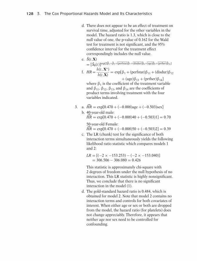
128 3. The Cox Proportional Hazards Model and Its Characteristics
d. There does not appear to be an effect of treatment onsurvival time, adjusted for the other variables in themodel. The hazard ratio is 1.3, which is close to thenull value of one, the p-value of 0.162 for the Waldtest for treatment is not significant, and the 95%confidence interval for the treatment effectcorrespondingly includes the null value.
e. S(t,X)= [S0(t)]exp[2β1+β5+(perfstat)β7+(disdur)β8+(age)β9+(prther)β10]
f. HR = h(t, X∗)h(t,X)
= exp[β1 + (perfstat)β11 + (disdur)β12
+ (age)β13 + (prther)β14]where β1 is the coefficient of the treatment variableand β11, β12, β13, and β14 are the coefficients ofproduct terms involving treatment with the fourvariables indicated.
3. a. HR = exp[0.470 + (−0.008)age + (−0.503)sex]b. 40-year-old male:
HR = exp[0.470 + (−0.008)40 + (−0.503)1] = 0.70
50-year-old Female:HR = exp[0.470 + (−0.008)50 + (−0.503)2] = 0.39
c. The LR (chunk) test for the significance of bothinteraction terms simultaneously yields the followinglikelihood ratio statistic which compares models 1and 2:
LR = [(−2 × −153.253) − (−2 × −153.040)]= 306.506 − 306.080 = 0.426
This statistic is approximately chi-square with2 degrees of freedom under the null hypothesis of nointeraction. This LR statistic is highly nonsignificant.Thus, we conclude that there is no significantinteraction in the model (1).
d. The gold-standard hazard ratio is 0.484, which isobtained for model 2. Note that model 2 contains nointeraction terms and controls for both covariates ofinterest. When either age or sex or both are droppedfrom the model, the hazard ratio (for platelets) doesnot change appreciably. Therefore, it appears thatneither age nor sex need to be controlled forconfounding.
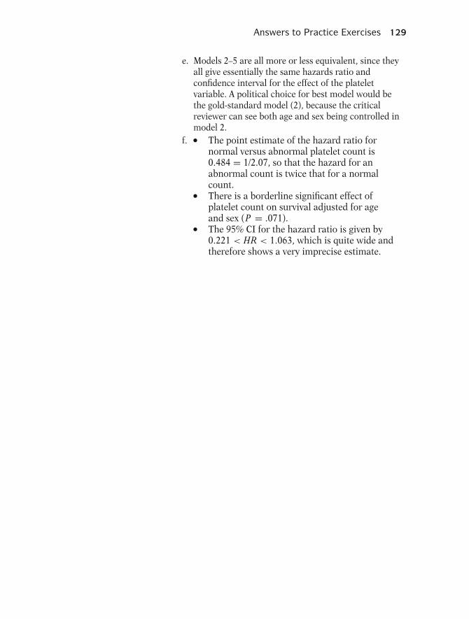
Answers to Practice Exercises 129
e. Models 2–5 are all more or less equivalent, since theyall give essentially the same hazards ratio andconfidence interval for the effect of the plateletvariable. A political choice for best model would bethe gold-standard model (2), because the criticalreviewer can see both age and sex being controlled inmodel 2.
f. � The point estimate of the hazard ratio fornormal versus abnormal platelet count is0.484 = 1/2.07, so that the hazard for anabnormal count is twice that for a normalcount.� There is a borderline significant effect ofplatelet count on survival adjusted for ageand sex (P = .071).� The 95% CI for the hazard ratio is given by0.221 < HR < 1.063, which is quite wide andtherefore shows a very imprecise estimate.
4 Evaluatingthe Propor-tionalHazardsAssumption
131

132 4. Evaluating the Proportional Hazards Assumption
Introduction We begin with a brief review of the characteristics of the Coxproportional hazards (PH) model. We then give an overviewof three methods for checking the PH assumption: graphi-cal, goodness-of-fit (GOF), and time-dependent variable ap-proaches.
We then focus on each of the above approaches, starting withgraphical methods. The most popular graphical approach in-volves the use of “log–log” survival curves. A second graphicalapproach involves the comparison of “observed” with “ex-pected” survival curves.
The GOF approach uses a test statistic or equivalent p-valueto assess the significance of the PH assumption. We illustratethis test and describe some of its advantages and drawbacks.
Finally, we discuss the use of time-dependent variables in anextended Cox model as a third method for checking the PHassumption. A more detailed description of the use of time-dependent variables is provided in Chapter 6.
AbbreviatedOutline
The outline below gives the user a preview of the material tobe covered by the presentation. A detailed outline for reviewpurposes follows the presentation.
I. Background (pages 134–135)II. Checking the PH assumption: Overview
(pages 135–137)III. Graphical approach 1: log–log plots
(pages 137–145)IV. Graphical approach 2: observed versus expected
plots (pages 145–150)V. The goodness-of-fit (GOF) testing approach
(pages 151–153)VI. Assessing the PH assumption using
time-dependent covariates (pages 153–157)

Objectives 133
Objectives Upon completing this chapter, the learner should be able to:
1. State or recognize three general approaches for evaluatingthe PH assumption.
2. Summarize how log–log survival curves may be used toassess the PH assumption.
3. Summarize how observed versus expected plots may beused to assess the PH assumption.
4. Summarize how GOF tests may be used to assess the PHassumption.
5. Summarize how time-dependent variables may be usedto assess the PH assumption.
6. Describe—given survival data or computer output from asurvival analysis that uses a Cox PH model—how to assessthe PH assumption for one or more variables in the modelusing:a. a graphical approachb. the GOF approachc. an extended Cox model with time-dependent
covariates7. State the formula for an extended Cox model that pro-
vides a method for checking the PH assumption for oneor more of the time-independent variables in the model,given survival analysis data or computer output that usesa Cox PH model.

134 4. Evaluating the Proportional Hazards Assumption
Presentation
FOCUS
Evaluating PH:• graphical• goodness-of-fit• time-dependent variables
This presentation describes three approaches forevaluating the proportional hazards (PH) assump-tion of the Cox model—a graphical procedure, agoodness-of-fit testing procedure, and a procedurethat involves the use of time-dependent variables.
I. Background Recall from the previous chapter that the generalform of the Cox PH model gives an expression forthe hazard at time t for an individual with a givenspecification of a set of explanatory variables de-noted by the bold X.
The Cox model formula says that the hazard attime t is the product of two quantities. The firstof these, h0(t), is called the baseline hazard func-tion. The second quantity is the exponential ex-pression e to the linear sum of βi Xi , where thesum is over the p explanatory X variables.
Cox PH model:
h(t,X) = h0(t)e
p∑i=1
βi Xi
X = (X1, X2, . . . , X p) explanatory/predictor variables
h0(t) × e
p∑i=1
βi Xi
Baseline hazard Exponential
Involves t but Involves X ’s butnot X ’s not t (X ’s are time-
independent)
An important feature of this formula, which con-cerns the proportional hazards (PH) assumption,is that the baseline hazard is a function of t, butdoes not involve the X ’s, whereas the exponentialexpression involves the X ’s, but does not involve t.The X ’s here are called time-independent X ’s.
X’s involving t: time-dependent
Requires extended Cox model(no PH) ↑
Chapter 6
It is possible, nevertheless, to consider X ’s thatdo involve t. Such X ’s are called time-dependentvariables. If time-dependent variables are consid-ered, the Cox model form may still be used, butsuch a model no longer satisfies the PH assump-tion, and is called the extended Cox model. Wewill discuss this extended Cox model in Chapter 6of this series.
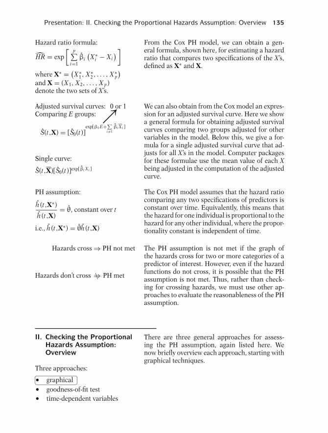
Presentation: II. Checking the Proportional Hazards Assumption: Overview 135
Hazard ratio formula:
HR = exp[ p∑
i=1βi
(X ∗
i − Xi) ]
where X∗ = (X ∗
1, X ∗2, . . . , X ∗
p
)and X = (X1, X2, . . . , X p)denote the two sets of X ’s.
From the Cox PH model, we can obtain a gen-eral formula, shown here, for estimating a hazardratio that compares two specifications of the X ’s,defined as X∗ and X.
Adjusted survival curves: 0 or 1Comparing E groups: ↗
S(t,X) = [S0(t)]exp[β1 E+∑
i �=1βi X i ]
We can also obtain from the Cox model an expres-sion for an adjusted survival curve. Here we showa general formula for obtaining adjusted survivalcurves comparing two groups adjusted for othervariables in the model. Below this, we give a for-mula for a single adjusted survival curve that ad-justs for all X ’s in the model. Computer packagesfor these formulae use the mean value of each Xbeing adjusted in the computation of the adjustedcurve.
Single curve:
S(t,X)[S0(t)]exp[βi Xi ]
PH assumption:
h (t,X∗)
h (t,X)= θ, constant over t
i.e., h (t,X∗) = θh (t,X)
The Cox PH model assumes that the hazard ratiocomparing any two specifications of predictors isconstant over time. Equivalently, this means thatthe hazard for one individual is proportional to thehazard for any other individual, where the propor-tionality constant is independent of time.
Hazards cross ⇒ PH not met
Hazards don’t cross ⇒\ PH met
The PH assumption is not met if the graph ofthe hazards cross for two or more categories of apredictor of interest. However, even if the hazardfunctions do not cross, it is possible that the PHassumption is not met. Thus, rather than check-ing for crossing hazards, we must use other ap-proaches to evaluate the reasonableness of the PHassumption.
II. Checking the ProportionalHazards Assumption:Overview
There are three general approaches for assess-ing the PH assumption, again listed here. Wenow briefly overview each approach, starting withgraphical techniques.
Three approaches:� graphical
��
�� goodness-of-fit test� time-dependent variables
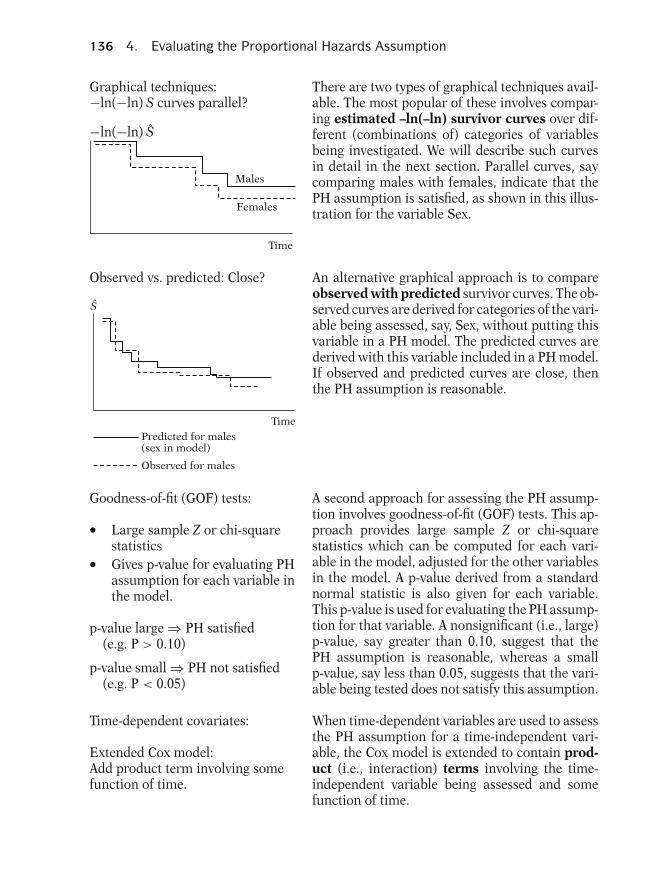
136 4. Evaluating the Proportional Hazards Assumption
Graphical techniques:−ln(−ln) S curves parallel?
−ln(−ln) S
Time
Females
Males
There are two types of graphical techniques avail-able. The most popular of these involves compar-ing estimated –ln(–ln) survivor curves over dif-ferent (combinations of) categories of variablesbeing investigated. We will describe such curvesin detail in the next section. Parallel curves, saycomparing males with females, indicate that thePH assumption is satisfied, as shown in this illus-tration for the variable Sex.
Observed vs. predicted: Close?
S
Time
Predicted for males(sex in model)
Observed for males
An alternative graphical approach is to compareobserved with predicted survivor curves. The ob-served curves are derived for categories of the vari-able being assessed, say, Sex, without putting thisvariable in a PH model. The predicted curves arederived with this variable included in a PH model.If observed and predicted curves are close, thenthe PH assumption is reasonable.
Goodness-of-fit (GOF) tests:
� Large sample Z or chi-squarestatistics� Gives p-value for evaluating PHassumption for each variable inthe model.
p-value large ⇒ PH satisfied(e.g. P > 0.10)
p-value small ⇒ PH not satisfied(e.g. P < 0.05)
A second approach for assessing the PH assump-tion involves goodness-of-fit (GOF) tests. This ap-proach provides large sample Z or chi-squarestatistics which can be computed for each vari-able in the model, adjusted for the other variablesin the model. A p-value derived from a standardnormal statistic is also given for each variable.This p-value is used for evaluating the PH assump-tion for that variable. A nonsignificant (i.e., large)p-value, say greater than 0.10, suggest that thePH assumption is reasonable, whereas a smallp-value, say less than 0.05, suggests that the vari-able being tested does not satisfy this assumption.
Time-dependent covariates:
Extended Cox model:Add product term involving somefunction of time.
When time-dependent variables are used to assessthe PH assumption for a time-independent vari-able, the Cox model is extended to contain prod-uct (i.e., interaction) terms involving the time-independent variable being assessed and somefunction of time.

Presentation: III. Graphical Approach 1: Log–Log Plots 137
EXAMPLE
h(t, X) = h0(t) exp[β Sex + δ(Sex × t)]
δ ≠ 0 ⇒ PH assumption violated
For example, if the PH assumption is being as-sessed for Sex, a Cox model might be extended toinclude the variable “Sex × t” in addition to Sex. Ifthe coefficient of the product term turns out to besignificant, we can conclude that the PH assump-tion is violated for Sex.
GOF provides test statisticGraphical: subjectiveTime-dependent: computationally
cumbersomeGOF: global, may not detect
specific departures from PH
The GOF approach provides a single test statis-tic for each variable being assessed. This ap-proach is not as subjective as the graphical ap-proach nor as cumbersome computationally asthe time-dependent variable approach. Neverthe-less, a GOF test may be too “global” in that itmay not detect specific departures from the PHassumption that may be observed from the othertwo approaches.
III. Graphical Approach 1:Log–Log Plots
The two graphical approaches for checking the PHassumption are comparing log–log survival curvesand comparing observed versus expected survivalcurves. We first explain what a −ln −ln survivalcurve is and how it is used.
� log–log survival curves� observed versus expectedsurvival curves
log – log S = transformation of S= −ln(−ln S)
� ln S is negative ⇒ −(ln S) ispositive.� can’t take log of ln S, but can
take log of (−ln S).� −ln(−ln S) may be positive ornegative.
A log–log survival curve is simply a transforma-tion of an estimated survival curve that resultsfrom taking the natural log of an estimated sur-vival probability twice. Mathematically, we write alog–log curve as −ln(−ln S). Note that the log of aprobability such as S is always a negative number.Because we can only take logs of positive num-bers, we need to negate the first log before takingthe second log. The value for −ln(−ln S) may bepositive or negative, either of which is acceptable,because we are not taking a third log.1
1An equivalent way to write −ln(−ln S) is −ln(∫ t
0 h(u)du),where
∫ t0 h(u)du is called the “cumulative hazard” function.
This result follows from the formula S (t) = exp[− ∫ t0 h(u)du],
which relates the survivor function to the hazard function (seep. 14 in Chapter 1).
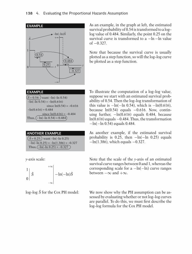
138 4. Evaluating the Proportional Hazards Assumption
t t
EXAMPLE
S
−∞
+∞
00
1
−0.327
0.4840.25
0.54
−ln(−ln)S
As an example, in the graph at left, the estimatedsurvival probability of 0.54 is transformed to a log–log value of 0.484. Similarly, the point 0.25 on thesurvival curve is transformed to a −ln −ln valueof −0.327.
Note that because the survival curve is usuallyplotted as a step function, so will the log–log curvebe plotted as a step function.
S = 0.54: want −ln(−ln 0.54)−ln(–ln 0.54) = −ln(0.616)
−ln(0.616) = 0.484since ln(0.54) = −0.616
since ln(0.616) = −0.484Thus, − ln(−ln 0.54) = 0.484
EXAMPLE To illustrate the computation of a log–log value,suppose we start with an estimated survival prob-ability of 0.54. Then the log–log transformation ofthis value is −ln(−ln 0.54), which is −ln(0.616),because ln(0.54) equals −0.616. Now, contin-uing further, −ln(0.616) equals 0.484, becauseln(0.616) equals −0.484. Thus, the transformation−ln(−ln 0.54) equals 0.484.
S = 0.25: want −ln(−ln 0.25)
−ln(−ln 0.25) = −ln(1.386) = −0.327Thus, −ln(–ln 0.25) = −0.327
ANOTHER EXAMPLE As another example, if the estimated survivalprobability is 0.25, then −ln(−ln 0.25) equals−ln(1.386), which equals −0.327.
y-axis scale:
1
0
∣∣∣∣∣+∞
S
−∞
∣∣∣∣∣∣∣∣ −ln(−ln)S
Note that the scale of the y-axis of an estimatedsurvival curve ranges between 0 and 1, whereas thecorresponding scale for a −ln(−ln) curve rangesbetween −∞ and +∞.
log–log S for the Cox PH model: We now show why the PH assumption can be as-sessed by evaluating whether or not log–log curvesare parallel. To do this, we must first describe thelog–log formula for the Cox PH model.

Presentation: III. Graphical Approach 1: Log–Log Plots 139
Cox PH hazard function:
h(t,X) = h0(t)e
p∑j=1
β j X j
↓ From math
Cox PH survival function:
S(t,X) = [S0(t)]e
p∑j=1
βj X j
↗Baseline survival function.
We start with the formula for the survival curvethat corresponds to the hazard function for theCox PH model. Recall that there is a mathemati-cal relationship between any hazard function andits corresponding survival function. We thereforecan obtain the formula shown here for the sur-vival curve for the Cox PH model. In this formula,the expression S0(t) denotes the baseline survivalfunction that corresponds to the baseline hazardfunction h0(t).
log–log ⇒ takes logs twice
log #1:
The log–log formula requires us to take logs of thissurvival function twice. The first time we take logswe get the expression shown here.
ln S(t,X) = e
p∑i=1
βi Xi × ln S0(t)0 ≤ S(t,X) ≤ 1
ln(probability) = negative value,so ln S(t,X) and ln S0(t) arenegative.
But −ln S(t,X) is positive, whichallows us to take logs again.
Now since S(t,X) denotes a survival probability, itsvalue for any t and any specification of the vectorX will be some number between 0 and 1. It followsthat the natural log of any number between 0 and1 is a negative number, so that the log of S(t, X) aswell as the log of S0(t) are both negative numbers.This is why we have to put a minus sign in front ofthis expression before we can take logs a secondtime, because there is no such thing as the log ofa negative number.
log #2:
ln[−ln S(t, X)]
= ln
[− e
p∑i=1
βi Xi × ln S0(t)
]
= ln
[e
p∑i=1
βi Xi
]+ ln[−ln S0(t)]
=p∑
i=1
βi Xi + ln[−ln S0(t)]
Thus, when taking the second log, we must obtainthe log of −ln S(t,X), as shown here. After usingsome algebra, this expression can be rewritten asthe sum of two terms, one of which is the linearsum of the βi Xi and the other is the log of thenegative log of the baseline survival function.
−ln[−ln S(t,X)]
= −p∑
i=1
βi Xi − ln[−ln S0(t)]
orln[−ln S(t, X)]
= +p∑
i=1
βi Xi + ln[−ln S(t)]
This second log may be either positive or nega-tive, and we aren’t taking any more logs, so weactually don’t have to take a second negative. How-ever, for consistency’s sake, a common practice isto put a minus sign in front of the second log to ob-tain the −ln −ln expression shown here. Neverthe-less, some software packages do not use a secondminus sign.

140 4. Evaluating the Proportional Hazards Assumption
Two individuals:X1 = (X11, X12, . . . , X1p)X2 = (X21, X22, . . . , X2p)
Now suppose we consider two different specifica-tions of the X vector, corresponding to two differ-ent individuals, X1 and X2.⎧⎪⎪⎪⎪⎪⎪⎪⎨⎪⎪⎪⎪⎪⎪⎪⎩
−ln[−ln S(t,X1)]
= −p∑
i=1βi X1i −ln[−ln S0(t)]
−ln[−ln S(t,X2)]
= −p∑
i=1βi X2i −ln[−ln S0(t)]
Then the corresponding log–log curves for theseindividuals are given as shown here, where wehave simply substituted X1 and X2 for X in theprevious expression for the log–log curve for anyindividual X.
−ln[−ln S(t,X1)]− (−ln[−ln S(t, X2)])
=p∑
i=1
βi (X2i − X1i )
does not involve t
Subtracting the second log–log curve from the firstyields the expression shown here. This expressionis a linear sum of the differences in correspondingpredictor values for the two individuals. Note thatthe baseline survival function has dropped out, sothat the difference in log–log curves involves anexpression that does not involve time t.
−ln[−ln S(t,X1)]= −ln[−ln S(t, X2)]
+p∑
i=1βi (X2i − X1i )
Alternatively, using algebra, we can write theabove equation by expressing the log–log survivalcurve for individual X1 as the log–log curve forindividual X2 plus a linear sum term that is inde-pendent of t.
t
X2
X1
−ln[−ln S]∑βi(X2i − X1i)
The above formula says that if we use a Cox PHmodel and we plot the estimated log–log survivalcurves for individuals on the same graph, the twoplots would be approximately parallel. The dis-tance between the two curves is the linear expres-sion involving the differences in predictor values,which does not involve time. Note, in general, ifthe vertical distance between two curves is con-stant, then the curves are parallel.
Graphical approach using log–logplots: PH model is appropriate if“empirical” plots of log–log survivalcurves are parallel.
The parallelism of log–log survival plots for theCox PH model provides us with a graphical ap-proach for assessing the PH assumption. That is,if a PH model is appropriate for a given set of pre-dictors, one should expect that empirical plots oflog–log survival curves for different individualswill be approximately parallel.
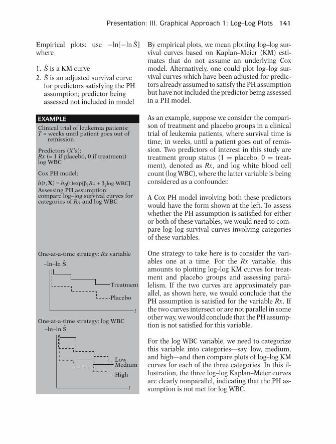
Presentation: III. Graphical Approach 1: Log–Log Plots 141
Empirical plots: use −ln[−ln S]where
1. S is a KM curve2. S is an adjusted survival curve
for predictors satisfying the PHassumption; predictor beingassessed not included in model
By empirical plots, we mean plotting log–log sur-vival curves based on Kaplan–Meier (KM) esti-mates that do not assume an underlying Coxmodel. Alternatively, one could plot log–log sur-vival curves which have been adjusted for predic-tors already assumed to satisfy the PH assumptionbut have not included the predictor being assessedin a PH model.
Clinical trial of leukemia patients:T = weeks until patient goes out of remission
Predictors (X ’s):Rx (= 1 if placebo, 0 if treatment)log WBC
Cox PH model:
EXAMPLE
Assessing PH assumption:compare log−log survival curves forcategories of Rx and log WBC
h(t,X) = h0(t)exp[β1Rx + β2log WBC]
One-at-a-time strategy: log WBC
LowMedium
High
t
−ln−ln S
Placebo
Treatment
t
−ln−ln S
One-at-a-time strategy: Rx variable
ˆ
ˆ
As an example, suppose we consider the compari-son of treatment and placebo groups in a clinicaltrial of leukemia patients, where survival time istime, in weeks, until a patient goes out of remis-sion. Two predictors of interest in this study aretreatment group status (1 = placebo, 0 = treat-ment), denoted as Rx, and log white blood cellcount (log WBC), where the latter variable is beingconsidered as a confounder.
A Cox PH model involving both these predictorswould have the form shown at the left. To assesswhether the PH assumption is satisfied for eitheror both of these variables, we would need to com-pare log–log survival curves involving categoriesof these variables.
One strategy to take here is to consider the vari-ables one at a time. For the Rx variable, thisamounts to plotting log–log KM curves for treat-ment and placebo groups and assessing paral-lelism. If the two curves are approximately par-allel, as shown here, we would conclude that thePH assumption is satisfied for the variable Rx. Ifthe two curves intersect or are not parallel in someother way, we would conclude that the PH assump-tion is not satisfied for this variable.
For the log WBC variable, we need to categorizethis variable into categories—say, low, medium,and high—and then compare plots of log–log KMcurves for each of the three categories. In this il-lustration, the three log–log Kaplan–Meier curvesare clearly nonparallel, indicating that the PH as-sumption is not met for log WBC.
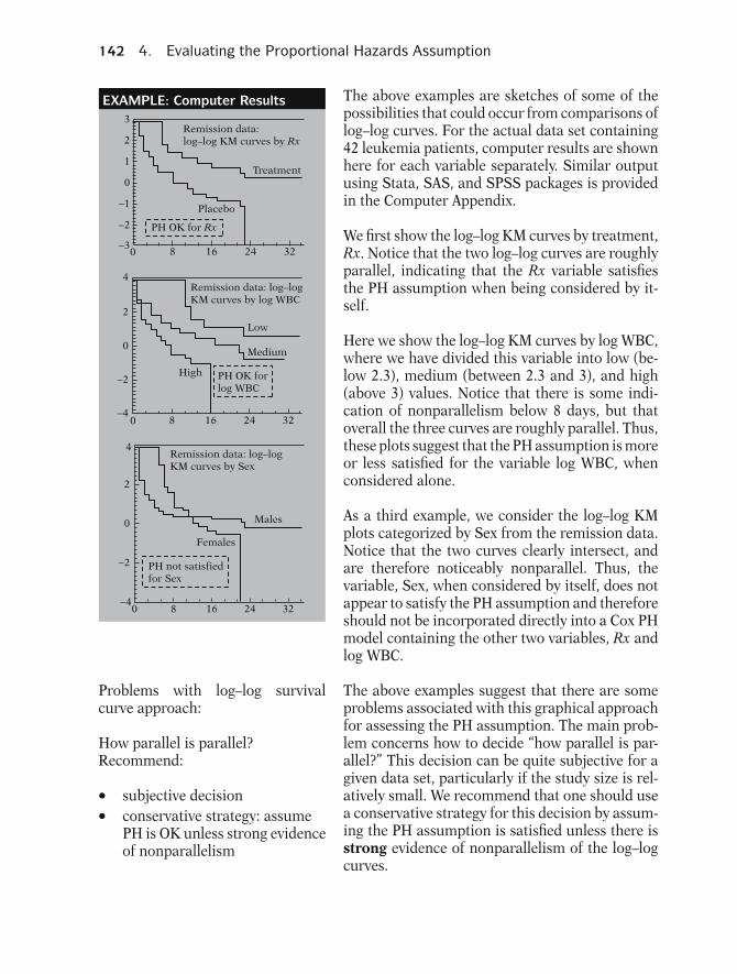
142 4. Evaluating the Proportional Hazards Assumption
3
2
1
0
−1
−2
−30 8 16 24 32
Remission data:log–log KM curves by Rx
Treatment
Placebo
PH OK for Rx
EXAMPLE: Computer Results
4
2
0
−2
−40 8 16 24 32
Remission data: log–log KM curves by log WBC
Low
Medium
High PH OK forlog WBC
−2
−40 8 16 24 32
4
2
0
Remission data: log–log KM curves by Sex
PH not satisfiedfor Sex
Females
Males
The above examples are sketches of some of thepossibilities that could occur from comparisons oflog–log curves. For the actual data set containing42 leukemia patients, computer results are shownhere for each variable separately. Similar outputusing Stata, SAS, and SPSS packages is providedin the Computer Appendix.
We first show the log–log KM curves by treatment,Rx. Notice that the two log–log curves are roughlyparallel, indicating that the Rx variable satisfiesthe PH assumption when being considered by it-self.
Here we show the log–log KM curves by log WBC,where we have divided this variable into low (be-low 2.3), medium (between 2.3 and 3), and high(above 3) values. Notice that there is some indi-cation of nonparallelism below 8 days, but thatoverall the three curves are roughly parallel. Thus,these plots suggest that the PH assumption is moreor less satisfied for the variable log WBC, whenconsidered alone.
As a third example, we consider the log–log KMplots categorized by Sex from the remission data.Notice that the two curves clearly intersect, andare therefore noticeably nonparallel. Thus, thevariable, Sex, when considered by itself, does notappear to satisfy the PH assumption and thereforeshould not be incorporated directly into a Cox PHmodel containing the other two variables, Rx andlog WBC.
Problems with log–log survivalcurve approach:
How parallel is parallel?Recommend:
� subjective decision� conservative strategy: assumePH is OK unless strong evidenceof nonparallelism
The above examples suggest that there are someproblems associated with this graphical approachfor assessing the PH assumption. The main prob-lem concerns how to decide “how parallel is par-allel?” This decision can be quite subjective for agiven data set, particularly if the study size is rel-atively small. We recommend that one should usea conservative strategy for this decision by assum-ing the PH assumption is satisfied unless there isstrong evidence of nonparallelism of the log–logcurves.
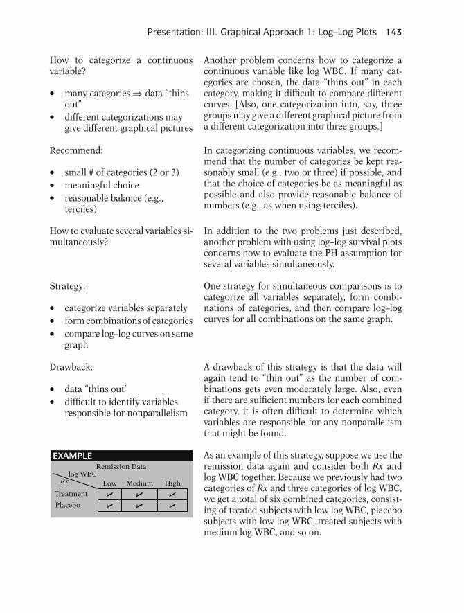
Presentation: III. Graphical Approach 1: Log–Log Plots 143
How to categorize a continuousvariable?
� many categories ⇒ data “thinsout”� different categorizations maygive different graphical pictures
Another problem concerns how to categorize acontinuous variable like log WBC. If many cat-egories are chosen, the data “thins out” in eachcategory, making it difficult to compare differentcurves. [Also, one categorization into, say, threegroups may give a different graphical picture froma different categorization into three groups.]
Recommend:
� small # of categories (2 or 3)� meaningful choice� reasonable balance (e.g.,terciles)
In categorizing continuous variables, we recom-mend that the number of categories be kept rea-sonably small (e.g., two or three) if possible, andthat the choice of categories be as meaningful aspossible and also provide reasonable balance ofnumbers (e.g., as when using terciles).
How to evaluate several variables si-multaneously?
In addition to the two problems just described,another problem with using log–log survival plotsconcerns how to evaluate the PH assumption forseveral variables simultaneously.
Strategy:
� categorize variables separately� form combinations of categories� compare log–log curves on samegraph
One strategy for simultaneous comparisons is tocategorize all variables separately, form combi-nations of categories, and then compare log–logcurves for all combinations on the same graph.
Drawback:
� data “thins out”� difficult to identify variablesresponsible for nonparallelism
A drawback of this strategy is that the data willagain tend to “thin out” as the number of com-binations gets even moderately large. Also, evenif there are sufficient numbers for each combinedcategory, it is often difficult to determine whichvariables are responsible for any nonparallelismthat might be found.
Remission Data
Low Medium Highlog WBC
Rx
Treatment
Placebo
EXAMPLE As an example of this strategy, suppose we use theremission data again and consider both Rx andlog WBC together. Because we previously had twocategories of Rx and three categories of log WBC,we get a total of six combined categories, consist-ing of treated subjects with low log WBC, placebosubjects with low log WBC, treated subjects withmedium log WBC, and so on.

144 4. Evaluating the Proportional Hazards Assumption
EXAMPLE (continued)
Log–log KM curves by six combinations of Rx by log WBC
3
2
1
0
−1
−2
−30 8 16 24
6
6
5
5 3 2
2
4
4
3
Plots suggest PH not satisfied. However, the study is small, i.e., plots are unreliable.
ˆThe computer results are shown here for the log–log curves corresponding to each of the six com-binations of Rx with log WBC. Notice that thereare several points of intersection among the sixcurves. Therefore, these results suggest that thePH assumption is not satisfied when consideringRx and log WBC together.
However, the sample sizes used to estimate thesecurves are quite small, ranging between four sub-jects for group 4 (Rx = 1, log WBC = low) totwelve subjects for group 6 (Rx = 1, log WBC =high), with the total study size being 42. Thus, forthis small study, the use of six log–log curves pro-vides unreliable information for assessing the PHassumption.
Alternative strategy:Adjust for predictors alreadysatisfying PH assumption, i.e., useadjusted log−log S curves
An alternative graphical strategy for consideringseveral predictors together is to assess the PH as-sumption for one predictor adjusted for other pre-dictors that are assumed to satisfy the PH assump-tion. Rather than using Kaplan–Meier curves, thisinvolves a comparison of adjusted log–log survivalcurves.
EXAMPLERemission data:• compare Rx categories adjusted for log WBC• fit PH model for each Rx stratum• obtain adjusted survival curves using overall mean of log WBC
Log–log S curves for Rx groups using PH model adjusted for log WBC
−2
−1
0
1
2
3
0 8 16 24 32
Treatment
Placebo
As an example, again we consider the remissiondata and the predictors Rx and log WBC. To as-sess the PH assumption for Rx adjusted for logWBC, we would compare adjusted log–log survivalcurves for the two treatment categories, whereeach adjusted curve is derived from a PH modelcontaining log WBC as a predictor. In computingthe adjusted survival curve, we need to stratify thedata by treatment, fit a PH model in each stratum,and then obtain adjusted survival probabilities us-ing the overall mean log WBC in the estimated sur-vival curve formula for each stratum.
For the remission data example, the estimatedlog–log survival curves for the two treatmentgroups adjusted for log WBC are shown here. No-tice that these two curves are roughly parallel, in-dicating that the PH assumption is satisfied fortreatment.

Presentation: IV. Graphical Approach 2: Observed Versus Expected Plots 145
Log–log S curves for log WBC groups usingPH model adjusted for Rx
−2
−1
0
1
2
3
0 8 16 24 32
Medium
High
Low
(Rx = 0.5)
EXAMPLE (continued)
Remission data:Assess PH assumption for Sex:• use PH model containing Rx and log WBC• use Rx and log WBC in survival probability formula
Log–log S curves for Sex adjusted for Rx andlog WBC
1
2
3
4
5
6
7
0 8 16 24 32
Females
Males
As another example, we consider adjusted log–logsurvival curves for three categories of log WBC, ad-justed for the treatment status (Rx) variable. Theadjusted survival probabilities in this case use theoverall mean Rx score, i.e., 0.5, the proportion ofthe 42 total subjects that are in the placebo group(i.e., half the subjects have a score of Rx = 1).
The three log–log curves adjusted for treatmentstatus are shown here. Although two of thesecurves intersect early in follow-up, they do not sug-gest a strong departure from parallelism overall,suggesting that the PH assumption is reasonablefor log WBC, after adjusting for treatment status.
As a third example, again using the remission data,we assess the PH assumption for Sex, adjusting forboth treatment status and log WBC in the model.This involves obtaining log–log survival curves formales and females separately, using a PH modelthat contains both treatment status and log WBC.The adjustment uses the overall mean treatmentscore and the overall mean log WBC score in theformula for the estimated survival probability.
The estimated log–log survival curves for Sex, ad-justed for treatment and log WBC are shown here.These curves clearly cross, indicating that the PHassumption is not satisfied for Sex, after adjustingfor treatment and log WBC.
1. log–log survival curves✓
2. observed versus expectedsurvival curves
We have thus described and illustrated one of thetwo graphical approaches for checking the PH as-sumption, that is, using log–log survival plots. Inthe next section, we describe an alternative ap-proach that compares “observed” with “expected”survival curves.
IV. Graphical Approach 2:Observed VersusExpected Plots
The use of observed versus expected plots to as-sess the PH assumption is the graphical analog ofthe goodness-of-fit (GOF) testing approach to bedescribed later, and is therefore a reasonable alter-native to the log–log survival curve approach.Graphical analog of GOF test

146 4. Evaluating the Proportional Hazards Assumption
Two strategies:
1. One-at-a-time: uses KM curves toobtain observed plots
2. Adjusting for other variables:uses stratified Cox PH model toobtain observed plots (seeChapter 5)
As with the log–log approach, the observed versusexpected approach may be carried out using ei-ther or both of two strategies—(1) assessing thePH assumption for variables one-at-a-time, or (2)assessing the PH assumption after adjusting forother variables. The strategy which adjusts forother variables uses a stratified Cox PH model toform observed plots, where the PH model containsthe variables to be adjusted and the stratified vari-able is the predictor being assessed. The stratifiedCox procedure is described in Chapter 5.
Here, we describe only the one-at-a-time strat-egy, which involves using KM curves to obtain ob-served plots.
One-at-a-time:
� stratify data by categories ofpredictor� obtain KM curves for eachcategory
Using the one-at-a-time strategy, we first muststratify our data by categories of the predictor tobe assessed. We then obtain observed plots by de-riving the KM curves separately for each category.
1
0.8
0.6
0.4
0.2
0
1
0.8
0.6
0.4
0.2
0
0 8 16 24 32
0 8 16 24 32
Placebo
Placebo
Treatment
Treatment
S
S
KM (Observed) Plots by Rx Group
Weeks
Weeks
Expected Survival Plots by Rx GroupUsing PH Model
h(t, X) = h0(t) e
S = [S0(t)]
EXAMPLE: Remission Data
exp[β,Rx]
β1Rx
As an example, for the remission data on 42leukemia patients we have illustrated earlier, theKM plots for the treatment and placebo groups,with 21 subjects in each group, are shown here.These are the “observed” plots.
To obtain “expected” plots, we fit a Cox PH modelcontaining the predictor being assessed. We ob-tain expected plots by separately substituting thevalue for each category of the predictor into theformula for the estimated survival curve, therebyobtaining a separate estimated survival curve foreach category.
As an example, again using the remission data, wefit the Cox PH model with Rx as its only variable.Using the corresponding survival curve formulafor this Cox model, as given in the box at the left,we then obtain separate expected plots by substi-tuting the values of 0 (for treatment group) and 1(for placebo group). The expected plots are shownhere.

Presentation: IV. Graphical Approach 2: Observed Versus Expected Plots 147
Observed Versus Expected Plots by Rx
EXAMPLE (continued)
S1
0.8
0.6
0.4
0.2
00
8 16 24 32
Placebo
Treatment
ExpectedObserved
To compare observed with expected plots we thenput both sets of plots on the same graph as shownhere.
If observed and expected plots are:
� close, complies with PHassumption� discrepant, PH assumptionviolated
If for each category of the predictor being as-sessed, the observed and expected plots are “close”to one another, we then can conclude that the PHassumption is satisfied. If, however, one or morecategories show quite discrepant observed and ex-pected plots, we conclude that the PH assumptionis violated.
EXAMPLE: Remission Data (continued)
Observed and expected plots are closefor each treatment group.
Conclude PH assumption not violated.
For the example shown above, observed and ex-pected curves appear to be quite close for eachtreatment group. Thus, we would conclude usingthis graphical approach that the treatment vari-able satisfies the PH assumption.
Drawback: How close is close?
Recommend: PH not satisfied onlywhen plots are strongly discrepant.
An obvious drawback to this graphical approachis deciding “how close is close” when comparingobserved versus expected curves for a given cat-egory. This is analogous to deciding “how par-allel is parallel” when comparing log–log sur-vival curves. Here, we recommend that the PHassumption be considered as not satisfied onlywhen observed and expected plots are stronglydiscrepant.
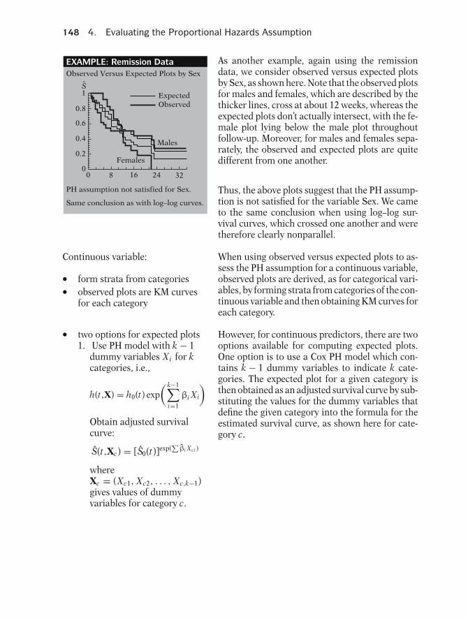
148 4. Evaluating the Proportional Hazards Assumption
Observed Versus Expected Plots by Sex
PH assumption not satisfied for Sex.
Same conclusion as with log–log curves.
EXAMPLE: Remission Data
S1
0.8
0.6
0.4
0.2
00
8 16 24 32
ExpectedObserved
Females
Males
As another example, again using the remissiondata, we consider observed versus expected plotsby Sex, as shown here. Note that the observed plotsfor males and females, which are described by thethicker lines, cross at about 12 weeks, whereas theexpected plots don’t actually intersect, with the fe-male plot lying below the male plot throughoutfollow-up. Moreover, for males and females sepa-rately, the observed and expected plots are quitedifferent from one another.
Thus, the above plots suggest that the PH assump-tion is not satisfied for the variable Sex. We cameto the same conclusion when using log–log sur-vival curves, which crossed one another and weretherefore clearly nonparallel.
Continuous variable:
� form strata from categories� observed plots are KM curvesfor each category
When using observed versus expected plots to as-sess the PH assumption for a continuous variable,observed plots are derived, as for categorical vari-ables, by forming strata from categories of the con-tinuous variable and then obtaining KM curves foreach category.
� two options for expected plots1. Use PH model with k − 1
dummy variables Xi for kcategories, i.e.,
h(t,X) = h0(t) exp( k−1∑
i=1
βi Xi
)Obtain adjusted survivalcurve:
S(t,Xc) = [S0(t)]exp(∑
βi Xci )
whereXc = (Xc1, Xc2, . . . , Xc,k−1)gives values of dummyvariables for category c.
However, for continuous predictors, there are twooptions available for computing expected plots.One option is to use a Cox PH model which con-tains k − 1 dummy variables to indicate k cate-gories. The expected plot for a given category isthen obtained as an adjusted survival curve by sub-stituting the values for the dummy variables thatdefine the given category into the formula for theestimated survival curve, as shown here for cate-gory c.
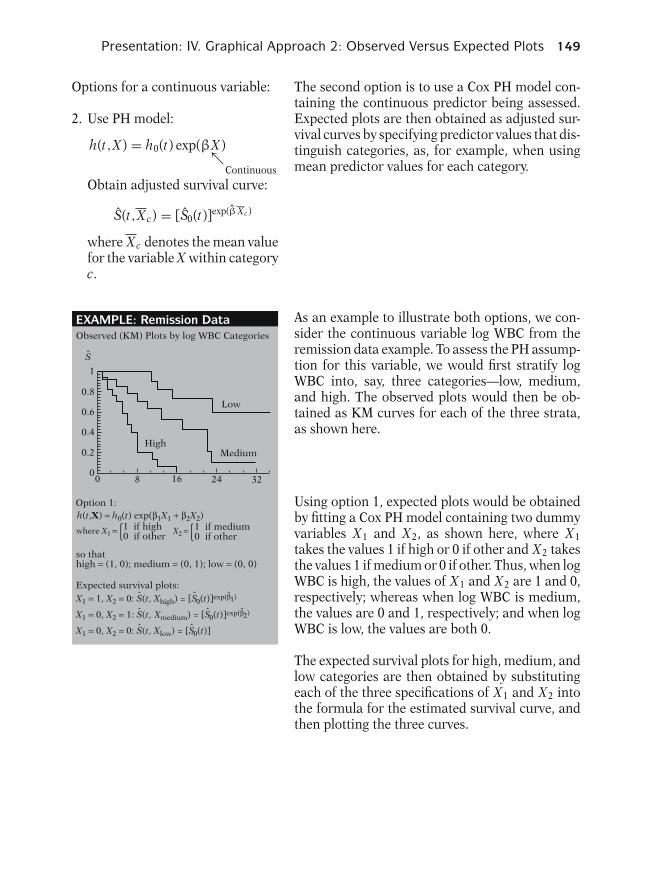
Presentation: IV. Graphical Approach 2: Observed Versus Expected Plots 149
Options for a continuous variable:
2. Use PH model:
h(t,X ) = h0(t) exp(βX )↖Continuous
Obtain adjusted survival curve:
S(t,X c) = [S0(t)]exp(βX c)
where X c denotes the mean valuefor the variable X within categoryc.
The second option is to use a Cox PH model con-taining the continuous predictor being assessed.Expected plots are then obtained as adjusted sur-vival curves by specifying predictor values that dis-tinguish categories, as, for example, when usingmean predictor values for each category.
Observed (KM) Plots by log WBC Categories
EXAMPLE: Remission Data
Option 1:h(t,X) = h0(t) exp(β1X1 + β2X2)
where X1 = {1 if high0 if other
X2 = {1 if medium0 if other
so thathigh = (1, 0); medium = (0, 1); low = (0, 0)
Expected survival plots:X1 = 1, X2 = 0: S(t, Xhigh) = [S0(t)]exp(β1)
X1 = 0, X2 = 1: S(t, Xmedium) = [S0(t)]exp(β2)
X1 = 0, X2 = 0: S(t, Xlow) = [S0(t)]
S
1
0.8
0.6
0.4
0.2
00
8 16 24 32
Low
HighMedium
As an example to illustrate both options, we con-sider the continuous variable log WBC from theremission data example. To assess the PH assump-tion for this variable, we would first stratify logWBC into, say, three categories—low, medium,and high. The observed plots would then be ob-tained as KM curves for each of the three strata,as shown here.
Using option 1, expected plots would be obtainedby fitting a Cox PH model containing two dummyvariables X1 and X2, as shown here, where X1takes the values 1 if high or 0 if other and X2 takesthe values 1 if medium or 0 if other. Thus, when logWBC is high, the values of X1 and X2 are 1 and 0,respectively; whereas when log WBC is medium,the values are 0 and 1, respectively; and when logWBC is low, the values are both 0.
The expected survival plots for high, medium, andlow categories are then obtained by substitutingeach of the three specifications of X1 and X2 intothe formula for the estimated survival curve, andthen plotting the three curves.
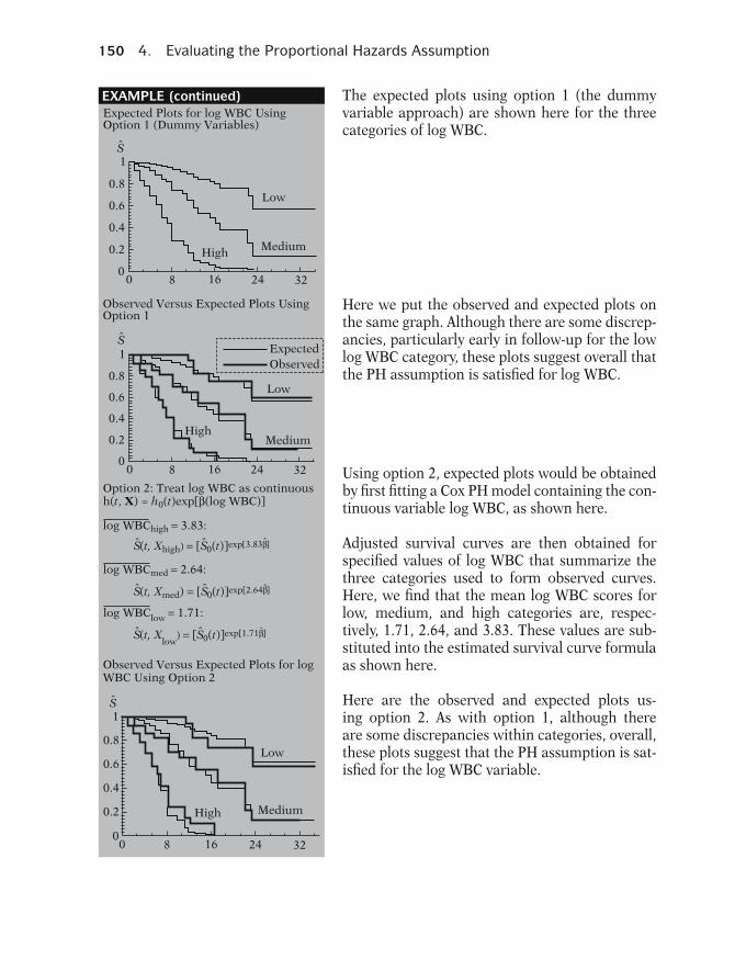
150 4. Evaluating the Proportional Hazards Assumption
1
0.8
0.6
0.4
0.2
00
8 16 24 32
Low
High Medium
S
1
0.8
0.6
0.4
0.2
00
8 16 24 32
S
Low
HighMedium
ExpectedObserved
Option 2: Treat log WBC as continuoush(t, X) = h0(t)exp[β(log WBC)]
log WBCmed = 2.64:
S(t, Xhigh) = [S0(t)]exp[3.83β]
log WBChigh = 3.83:
S(t, Xmed) = [S0(t)]exp[2.64β ]
log WBClow = 1.71:
Observed Versus Expected Plots Using Option 1
Expected Plots for log WBC Using Option 1 (Dummy Variables)
EXAMPLE (continued)
1
0.8
0.6
0.4
0.2
00
8 16 24 32
Low
High Medium
S
Observed Versus Expected Plots for logWBC Using Option 2
S(t, Xlow
) = [S0(t)]exp[1.71β]
The expected plots using option 1 (the dummyvariable approach) are shown here for the threecategories of log WBC.
Here we put the observed and expected plots onthe same graph. Although there are some discrep-ancies, particularly early in follow-up for the lowlog WBC category, these plots suggest overall thatthe PH assumption is satisfied for log WBC.
Using option 2, expected plots would be obtainedby first fitting a Cox PH model containing the con-tinuous variable log WBC, as shown here.
Adjusted survival curves are then obtained forspecified values of log WBC that summarize thethree categories used to form observed curves.Here, we find that the mean log WBC scores forlow, medium, and high categories are, respec-tively, 1.71, 2.64, and 3.83. These values are sub-stituted into the estimated survival curve formulaas shown here.
Here are the observed and expected plots us-ing option 2. As with option 1, although thereare some discrepancies within categories, overall,these plots suggest that the PH assumption is sat-isfied for the log WBC variable.
Presentation: V. The Goodness of Fit (GOF) Testing Approach 151
V. The Goodness of Fit (GOF)Testing Approach
The GOF testing approach is appealing because itprovides a test statistic and p-value for assessingthe PH assumption for a given predictor of inter-est. Thus, the researcher can make a more objec-tive decision using a statistical test than is typicallypossible when using either of the two graphical ap-proaches described above.
Statistical test appealing
� Provides p-value� More objective decision thanwhen using graphical approach
Test of Harrel and Lee (1986)
� Variation of test of Schoenfeld� Uses Schoenfeld residuals
A number of different tests for assessing the PH as-sumption have been proposed in the literature. Wepresent the test of Harrel and Lee (1986), a varia-tion of a test originally proposed by Schoenfeld(1982) and based on the residuals defined bySchoenfeld, now called the Schoenfeld residuals.
Schoenfeld residuals defined for
� Each predictor in model� Every subject who has event
Consider Cox PH model
h(t) = h0(t) exp(β1RX+β2log WBC + β3SEX)
3 predictors −→ 3 Schoenfeldresiduals for eachsubject who hasevent
For each predictor in the model, Schoenfeld resid-uals are defined for every subject who has an event.For example, consider a Cox PH model with threepredictors: RX, LOGWBC, and SEX. Then thereare three Schoenfeld residuals defined for eachsubject who has an event, one for each of the threepredictors.
Schoenfeld residual for ith subjectfor LOGWBC
Observed LOGWBC– LOGWBC weighted average
Weights are other subjects’ hazard(from subjects still at risk)
Suppose subject i has an event at time tj. Thenher Schoenfeld residual for LOGWBC is her ob-served value of log white blood cell count minus aweighted average of the log white blood cell countsfor the other subjects still at risk at time tj. Theweights are each subject’s hazard.
Underlying idea of testIf PH holds then Schoenfeld residu-als uncorrelated with time
The idea behind the statistical test is that if thePH assumption holds for a particular covariatethen the Schoenfeld residuals for that covari-ate will not be related to survival time.
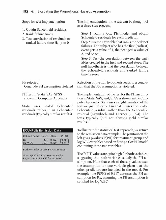
152 4. Evaluating the Proportional Hazards Assumption
Steps for test implementation
1. Obtain Schoenfeld residuals2. Rank failure times3. Test correlation of residuals to
ranked failure time H0: ρ = 0
The implementation of the test can be thought ofas a three-step process.
Step 1. Run a Cox PH model and obtainSchoenfeld residuals for each predictor.Step 2. Create a variable that ranks the order offailures. The subject who has the first (earliest)event gets a value of 1, the next gets a value of2, and so on.Step 3. Test the correlation between the vari-ables created in the first and second steps. Thenull hypothesis is that the correlation betweenthe Schoenfeld residuals and ranked failuretime is zero.
H0 rejectedConclude PH assumption violated
Rejection of the null hypothesis leads to a conclu-sion that the PH assumption is violated.
PH test in Stata, SAS, SPSSshown in Computer Appendix
Stata uses scaled Schoenfeldresiduals rather than Schoenfeldresiduals (typically similar results)
The implementation of the test for the PH assump-tion in Stata, SAS, and, SPSS is shown in the Com-puter Appendix. Stata uses a slight variation of thetest we just described in that it uses the scaledSchoenfeld residual rather than the Schoenfeldresidual (Grambsch and Therneau, 1994). Thetests typically (but not always) yield similarresults.
Column name Coeff. StErr. P(PH)
Both variables satisfy PH assumption.
Note: P(PH) = 0.917 assesses PH forRx, assuming PH OK for log WBC.
1.2941.604
0.4220.329
0.9170.944
Rxlog WBC
EXAMPLE: Remission Data To illustrate the statistical test approach, we returnto the remission data example. The printout on theleft gives p-values P(PH) for treatment group andlog WBC variables based on fitting a Cox PH modelcontaining these two variables.
The P(PH) values are quite high for both variables,suggesting that both variables satisfy the PH as-sumption. Note that each of these p-values teststhe assumption for one variable given that theother predictors are included in the model. Forexample, the P(PH) of 0.917 assesses the PH as-sumption for Rx, assuming the PH assumption issatisfied for log WBC.
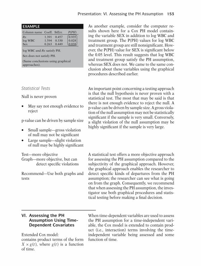
Presentation: VI. Assessing the PH Assumption 153
log WBC and Rx satisfy PH.
Sex does not satisfy PH.
(Same conclusions using graphicalapproaches).
1.3911.5940.263
0.4570.3300.449
0.9350.8280.038
Rxlog WBCSex
Column name Coeff. StErr. P(PH)
EXAMPLE As another example, consider the computer re-sults shown here for a Cox PH model contain-ing the variable SEX in addition to log WBC andtreatment group. The P(PH) values for log WBCand treatment group are still nonsignificant. How-ever, the P(PH) value for SEX is significant belowthe 0.05 level. This result suggests that log WBCand treatment group satisfy the PH assumption,whereas SEX does not. We came to the same con-clusion about these variables using the graphicalprocedures described earlier.
Statistical Tests An important point concerning a testing approachis that the null hypothesis is never proven with astatistical test. The most that may be said is thatthere is not enough evidence to reject the null. Ap-value can be driven by sample size. A gross viola-tion of the null assumption may not be statisticallysignificant if the sample is very small. Conversely,a slight violation of the null assumption may behighly significant if the sample is very large.
Null is never proven
� May say not enough evidence toreject
p-value can be driven by sample size
� Small sample—gross violationof null may not be significant� Large sample—slight violationof null may be highly significant
Test—more objectiveGraph—more objective, but can
detect specific violations
Recommend—Use both graphs andtests
A statistical test offers a more objective approachfor assessing the PH assumption compared to thesubjectivity of the graphical approach. However,the graphical approach enables the researcher todetect specific kinds of departures from the PHassumption; the researcher can see what is goingon from the graph. Consequently, we recommendthat when assessing the PH assumption, the inves-tigator use both graphical procedures and statis-tical testing before making a final decision.
VI. Assessing the PHAssumption Using Time-Dependent Covariates
When time-dependent variables are used to assessthe PH assumption for a time-independent vari-able, the Cox model is extended to contain prod-uct (i.e., interaction) terms involving the time-independent variable being assessed and somefunction of time.
Extended Cox model:contains product terms of the formX × g (t), where g (t) is a functionof time.

154 4. Evaluating the Proportional Hazards Assumption
One-at-a-time model:
h(t,X) = h0(t) exp[βX + δX × g (t)]
When assessing predictors one-at-a-time, the ex-tended Cox model takes the general form shownhere for the predictor X.
Some choices for g (t):g (t) = tg (t) = log t
g (t) ={
1 if t ≥ t00 if t < t0
(heavisidefunction)
One choice for the function g(t) is simply g(t) equalto t, so that the product term takes the form X × t.Other choices for g(t) are also possible, for exam-ple, log t.
H0: δ = 0Under H0, the model reduces to:
h(t,X) = h0(t) exp[βX ]
Using the above one-at-a-time model, we assessthe PH assumption by testing for the significanceof the product term. The null hypothesis is there-fore “δ equal to zero.” Note that if the null hypoth-esis is true, the model reduces to a Cox PH modelcontaining the single variable X.
Use either Wald statistic orlikelihood ratio statistic:X 2 with 1 df under H0
The test can be carried out using either a Waldstatistic or a likelihood ratio statistic. In eithercase, the test statistic has a chi-square distribu-tion with one degree of freedom under the nullhypothesis.
EXAMPLE h(t,X) = h0(t)exp[β1 Sex + β2 (Sex × t)]
β2 ≠ 0 ⇒ PH assumption violated
For example, if the PH assumption is being as-sessed for Sex, a Cox model might be extended toinclude the variable Sex × t in addition to Sex. Ifthe coefficient of the product term turns out to besignificant, we can conclude that the PH assump-tion is violated for Sex.2
Strategies for assessing PH:
� one-at-a-time� several predictorssimultaneously� for a given predictor adjusted forother predictors
In addition to a one-at-a-time strategy, the ex-tended Cox model can also be used to assess thePH assumption for several predictors simultane-ously as well as for a given predictor adjusted forother predictors in the model.
2In contrast, if the test for H0: β2 = 0 is nonsignificant, wecan conclude only that the particular version of the extendedCox model being considered is not supported by the data.
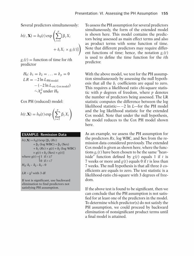
Presentation: VI. Assessing the PH Assumption 155
Several predictors simultaneously:
h(t, X) = h0(t) exp
(p∑
i=1
[βi Xi
+ δi Xi × gi (t)]
)gi (t) = function of time for ithpredictor
To assess the PH assumption for several predictorssimultaneously, the form of the extended modelis shown here. This model contains the predic-tors being assessed as main effect terms and alsoas product terms with some function of time.Note that different predictors may require differ-ent functions of time; hence, the notation gi (t)is used to define the time function for the ithpredictor.
H0: δ1 = δ2 = . . . = δp = 0L R = −2 ln LPH model
− (−2 ln Lext. Cox model)∼X 2
p under H0
Cox PH (reduced) model:
h(t,X) = h0(t) exp
(p∑
i=1
βi Xi
)
With the above model, we test for the PH assump-tion simultaneously by assessing the null hypoth-esis that all the δi coefficients are equal to zero.This requires a likelihood ratio chi-square statis-tic with p degrees of freedom, where p denotesthe number of predictors being assessed. The LRstatistic computes the difference between the loglikelihood statistic— −2 ln L—for the PH modeland the log likelihood statistic for the extendedCox model. Note that under the null hypothesis,the model reduces to the Cox PH model shownhere.
EXAMPLE: Remission Data
If test is significant, use backwardelimination to find predictors notsatisfying PH assumption.
h(t,X) = h0(t)exp [β1 (Rx)+ β2 (log WBC) + β3 (Sex)+ δ1 (Rx) × g(t) + δ2 (log WBC)× g(t) + δ3 (Sex) × g(t)]
H0: δ1 = δ2 = δ3 = 0
LR ∼ χ2 with 3 df
where g(t) = 1 if t ≥70 if t <7{
.
As an example, we assess the PH assumption forthe predictors Rx, log WBC, and Sex from the re-mission data considered previously. The extendedCox model is given as shown here, where the func-tions gi (t) have been chosen to be the same “heav-iside” function defined by g (t) equals 1 if t is7 weeks or more and g (t) equals 0 if t is less than7 weeks. The null hypothesis is that all three δ co-efficients are equals to zero. The test statistic is alikelihood-ratio chi-square with 3 degrees of free-dom.
If the above test is found to be significant, then wecan conclude that the PH assumption is not satis-fied for at least one of the predictors in the model.To determine which predictor(s) do not satisfy thePH assumption, we could proceed by backwardelimination of nonsignificant product terms untila final model is attained.
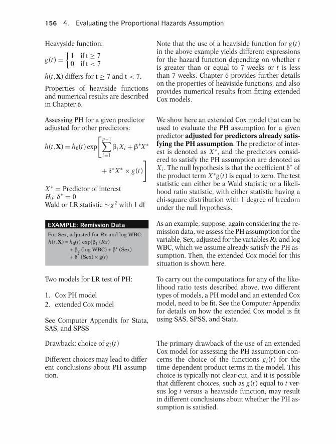
156 4. Evaluating the Proportional Hazards Assumption
Heavyside function:
g (t) ={
1 if t ≥ 70 if t < 7
h(t,X) differs for t ≥ 7 and t < 7.
Properties of heaviside functionsand numerical results are describedin Chapter 6.
Note that the use of a heaviside function for g (t)in the above example yields different expressionsfor the hazard function depending on whether tis greater than or equal to 7 weeks or t is lessthan 7 weeks. Chapter 6 provides further detailson the properties of heaviside functions, and alsoprovides numerical results from fitting extendedCox models.
Assessing PH for a given predictoradjusted for other predictors:
h(t,X) = h0(t) exp
[p−1∑i=1
βi Xi +β∗X ∗
+ δ∗ X ∗ × g (t)
]X ∗ = Predictor of interestH0: δ∗ = 0Wald or LR statistic ∼χ2 with 1 df
We show here an extended Cox model that can beused to evaluate the PH assumption for a givenpredictor adjusted for predictors already satis-fying the PH assumption. The predictor of inter-est is denoted as X ∗, and the predictors consid-ered to satisfy the PH assumption are denoted asXi . The null hypothesis is that the coefficient δ∗ ofthe product term X ∗g (t) is equal to zero. The teststatistic can either be a Wald statistic or a likeli-hood ratio statistic, with either statistic having achi-square distribution with 1 degree of freedomunder the null hypothesis.
For Sex, adjusted for Rx and log WBC:h(t,X) = h0(t) exp[β1 (Rx)
+ β2 (log WBC) + β* (Sex)+ δ* (Sex) × g(t)
EXAMPLE: Remission Data As an example, suppose, again considering the re-mission data, we assess the PH assumption for thevariable, Sex, adjusted for the variables Rx and logWBC, which we assume already satisfy the PH as-sumption. Then, the extended Cox model for thissituation is shown here.
Two models for LR test of PH:
1. Cox PH model2. extended Cox model
See Computer Appendix for Stata,SAS, and SPSS
To carry out the computations for any of the like-lihood ratio tests described above, two differenttypes of models, a PH model and an extended Coxmodel, need to be fit. See the Computer Appendixfor details on how the extended Cox model is fitusing SAS, SPSS, and Stata.
Drawback: choice of gi (t)
Different choices may lead to differ-ent conclusions about PH assump-tion.
The primary drawback of the use of an extendedCox model for assessing the PH assumption con-cerns the choice of the functions gi (t) for thetime-dependent product terms in the model. Thischoice is typically not clear-cut, and it is possiblethat different choices, such as g (t) equal to t ver-sus log t versus a heaviside function, may resultin different conclusions about whether the PH as-sumption is satisfied.

Presentation: VI. Assessing the PH Assumption 157
Chapter 6: Time-dependentcovariates
Further discussion of the use of time-dependentcovariates in an extended Cox model is providedin Chapter 6.
This presentation:Three methods for assessing PH.
i. graphicalii. GOF
iii. time-dependent covariates
Recommend using at least twomethods.
This presentation is now complete. We have de-scribed and illustrated three methods for assess-ing the PH assumption: graphical, goodness-of-fit (GOF), and time-dependent covariate methods.Each of these methods has both advantages anddrawbacks. We recommend that the researcheruse at least two of these approaches when assess-ing the PH assumption.
Chapters We suggest that the reader review this presenta-tion using the detailed outline that follows. Thenanswer the practice exercises and the test that fol-low.
The next Chapter (5) is entitled “The Stratified CoxProcedure.” There, we describe how to use a strat-ification procedure to fit a PH model when oneor more of the predictors do not satisfy the PHassumption.
1. Introduction to SurvivalAnalysis
2. Kaplan–Meier Survival Curvesand the Log–Rank Test
3. The Cox Proportional HazardsModel and Its Characteristics
✓ 4. Evaluating the ProportionalHazards Assumption
��
��
Next:
5. The Stratified Cox Procedure6. Extension of the Cox
Proportional Hazards Modelfor Time-Dependent Variables

158 4. Evaluating the Proportional Hazards Assumption
DetailedOutline
I. Background (pages 134–135)A. The formula for the Cox PH model:
h(t,X) = h0(t) exp[ p∑
i=1βi Xi
]B. Formula for hazard ratio comparing two
individuals,
X∗ = (X ∗1, X ∗
2, . . . , X ∗p) and X = (X1, X2, . . . , X p):
h(t,X∗)h(t,X)
= exp
[p∑
i=1
βi
(X ∗
i − Xi)]
C. Adjusted survival curves using the Cox PH model:
S(t,X) = [S0(t)]exp[∑
βi Xi ]
i. To graph S(t, X), must specify values for
X = (X1, X2, . . . , X p).
ii. To obtain “adjusted” survival curves, usually useoverall mean values for the X ’s being adjusted.
D. The meaning of the PH assumptioni. Hazard ratio formula shows that hazard ratio is
independent of time:
h (t,X∗)
h (t,X)= θ
ii. Hazard ratio for two X ’s are proportional:
h (t,X∗) = θh (t,X)
II. Checking the PH assumption: Overview (pages135–137)A. Three methods for checking the PH assumption:
i. Graphical: compare −ln −ln survival curves orobserved versus predicted curves.
ii. Goodness-of-fit test: use a large sample Zstatistic.
iii. Time-dependent covariates: use product (i.e.,interaction) terms of the form X × g (t).
B. Abbreviated illustrations of each method areprovided.
III. Graphical approach 1: log–log plots (pages 137–145)A. A log–log curve is a transformation of an estimated
survival curve, where the scale for a log–log curve is−∞ to +∞.

Detailed Outline 159
B. The log–log expression for the Cox model survivalcurve is given by
−ln[−lnS(t,X)] = −p∑
i=1
βi Xi −ln[−lnS0(t)]
C. For the Cox model, the log–log survival curve forindividual X1 can be written as the log–log curve forindividual X2 plus a linear sum term that isindependent of time t. This formula is given by−ln[−lnS(t,X1)]
= −ln[−lnS(t,X2)] +p∑
i=1
βi (X2i − X1i )
D. The above log–log formula can be used to check thePH assumption as follows: the PH model isappropriate if “empirical” plots of log–log survivalcurves are parallel.
E. Two kinds of empirical plots for −ln −ln S:i. S is a KM curve
ii. S is an adjusted survival curve where predictorbeing assessed is not included in the Coxregression model.
F. Several examples of log–log plots are provided usingremission data from a clinical trial of leukemiapatients.
G. Problems with log–log curves:i. How parallel is parallel?
ii. How to categorize a continuous variable?iii. How to evaluate several variables
simultaneously?H. Recommendation about problems:
i. Use small number of categories, meaningfulchoice, reasonable balance.
ii. With several variables, two options:a. Compare log–log curves from combinations of
categories.b. Adjust for predictors already satisfying PH
assumption.IV. Graphical approach 2: observed versus expected
plots (pages 145–150)A. Graphical analog of the GOF test.B. Two strategies
i. One-at-a-time: uses KM curves to obtainobserved plots.
ii. Adjusting for other variables: uses stratified CoxPH model to obtain observed plots.

160 4. Evaluating the Proportional Hazards Assumption
C. Expected plots obtained by fitting a Cox modelcontaining the predictor being assessed; substituteinto the fitted model the value for each category ofthe predictor to obtain the expected value for eachcategory.
D. If observed and expected plots are close, concludePH assumption is reasonable.
E. Drawback: how close is close?F. Recommend: conclude PH not satisfied only if plots
are strongly discrepant.G. Another drawback: what to do if assessing
continuous variable.H. Recommend for continuous variable:
i. Form strata from categories.ii. Observed plots are KM curves for each category.
iii. Two options for expected plots:a. Use PH model with k − 1 dummy variables
for k categories.b. Use PH model with continuous predictor and
specify predictor values that distinguishcategories.
V. The goodness-of-fit (GOF) testing approach (pages151–153)A. Appealing approach because
i. provides a test statistic (p-value).ii. researcher can make clear-cut decision.
B. Referencesi. methodological: Schoenfeld (1982), Harrel and
Lee (1986).ii. SAS and Stata use different GOF formulae.
C. The method:i. Schoenfeld residuals for each predictor uses a
chi-square statistic with 1 df.ii. Correlations between Schoenfeld’s residuals and
ranked failure times.iii. If p-value small, then departure from PH.
D. Examples using remission data.E. Drawbacks:
i. global test: may fail to detect a specific kind ofdeparture from PH; recommend using bothgraphical and GOF methods.
ii. several strategies to choose from, with no onestrategy clearly preferable (one-at-a-time, allvariables, each variable adjusted for others).

Practice Exercises 161
VI. Assessing the PH assumption (using time-dependent covariates) (pages 153–157)A. Use extended Cox model: contains product terms of
form X × g (t), where g (t) is function of time, e.g.,g (t) = t, or log t, or heaviside function.
B. One-at-a-time model:h(t,X) = h0(t) exp[βX + δg (t)].Test H0: δ = 0 using Wald or LR test (chi-squarewith 1 df).
C. Evaluating several predictors simultaneously:
h(t, X) = h0(t) exp
(p∑
i=1
[βi Xi + δi Xi gi (t)]
)where gi (t) is function of time for ith predictor. TestH0 : δ1 = δ2 = · · · = δp = 0 using LR (chi-square)test with p df.
D. Examples using remission data.E. Two computer programs, required for test:
i. Cox PH model program.ii. Extended Cox model program.
F. Drawback: choice of g (t) not always clear; differentchoices may lead to different conclusions about PHassumption.
PracticeExercises
The dataset “vets.dat” considers survival times in days for 137patients from the Veteran’s Administration Lung Cancer Trialcited by Kalbfleisch and Prentice in their text (The StatisticalAnalysis of Survival Time Data, Wiley, pp. 223–224, 1980). Theexposure variable of interest is treatment status (standard =1, test = 2). Other variables of interest as control variablesare cell type (four types, defined by dummy variables), perfor-mance status, disease duration, age, and prior therapy status.Failure status is defined by the status variable (0 if censored,1 if died). A complete list of the variables is given below.
Column 1: Treatment (standard = 1, test = 2)Column 2: Cell type 1 (large = 1, other = 0)Column 3: Cell type 2 (adeno = 1, other = 0)Column 4: Cell type 3 (small = 1, other = 0)Column 5: Cell type 4 (squamous = 1, other = 0)Column 6: Survival time (days)
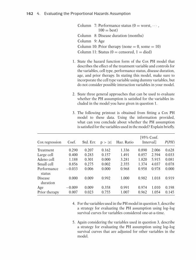
162 4. Evaluating the Proportional Hazards Assumption
Column 7: Performance status (0 = worst, · · · ,100 = best)
Column 8: Disease duration (months)Column 9: AgeColumn 10: Prior therapy (none = 0, some = 10)Column 11: Status (0 = censored, 1 = died)
1. State the hazard function form of the Cox PH model thatdescribes the effect of the treatment variable and controls forthe variables, cell type, performance status, disease duration,age, and prior therapy. In stating this model, make sure toincorporate the cell type variable using dummy variables, butdo not consider possible interaction variables in your model.
2. State three general approaches that can be used to evaluatewhether the PH assumption is satisfied for the variables in-cluded in the model you have given in question 1.
3. The following printout is obtained from fitting a Cox PHmodel to these data. Using the information provided,what can you conclude about whether the PH assumptionis satisfied for the variables used in the model? Explain briefly.
[95% Conf.Cox regression Coef. Std. Err. p > |z| Haz. Ratio Interval] P(PH)
Treatment 0.290 0.207 0.162 1.336 0.890 2.006 0.628Large cell 0.400 0.283 0.157 1.491 0.857 2.594 0.033Adeno cell 1.188 0.301 0.000 3.281 1.820 5.915 0.081Small cell 0.856 0.275 0.002 2.355 1.374 4.037 0.078Performance −0.033 0.006 0.000 0.968 0.958 0.978 0.000
statusDisease 0.000 0.009 0.992 1.000 0.982 1.018 0.919
durationAge −0.009 0.009 0.358 0.991 0.974 1.010 0.198Prior therapy 0.007 0.023 0.755 1.007 0.962 1.054 0.145
4. For the variables used in the PH model in question 3, describea strategy for evaluating the PH assumption using log–logsurvival curves for variables considered one-at-a-time.
5. Again considering the variables used in question 3, describea strategy for evaluating the PH assumption using log–logsurvival curves that are adjusted for other variables in themodel.

Practice Exercises 163
6. For the variable “performance status,” describe how youwould evaluate the PH assumption using observed versusexpected survival plots?
7. For the variable “performance status,” log–log plots whichcompare high (≥50) with low (<50) are given by the follow-ing graph. Based on this graph, what do you conclude aboutthe PH assumption with regard to this variable?
0−4
−2
0
2
4
6
200 400 600 800 1000
High PSLow PS
8. What are some of the drawbacks of using the log–log ap-proach for assessing the PH assumption and what do yourecommend to deal with these drawbacks?
9. For the variable “performance status,” observed versus ex-pected plots that compare high (≥50) with low (<50) aregiven by the following graph. Based on this graph, what doyou conclude about the PH assumption with regard to thisvariable?
00 200 400 600 800 1000
0.2
0.4
0.6
0.8
1Observed
Expected
Low
High
10. State the form of an extended Cox model that allows forthe one-at-a-time assessment of the PH assumption for thevariable “performance status,” and describe how you wouldcarry out a statistical test of the assumption for this variable.
11. State the form of an extended Cox model that allows for thesimultaneous assessment of the PH assumption for the vari-ables, treatment, cell type, performance status, disease du-ration, age, and prior therapy. For this model, describe howyou would carry out a statistical test of the PH assump-tion for these variables. Also, provide a strategy for assess-ing which of these variables satisfy the PH assumption andwhich do not using the extended Cox model approach.

164 4. Evaluating the Proportional Hazards Assumption
12. Using any of the information provided above and any addi-tional analyses that you perform with this dataset, what doyou conclude about which variables satisfy the PH assump-tion and which variables do not? In answering this question,summarize any additional analyses performed.
Test The following questions consider a dataset from a study byCaplehorn et al. (“Methadone Dosage and Retention of Pa-tients in Maintenance Treatment,” Med. J. Aust., 1991). Thesedata comprise the times in days spent by heroin addicts fromentry to departure from one of two methadone clinics. Thereare two additional covariates, namely, prison record and max-imum methadone dose, believed to affect the survival times.The dataset name is addicts.dat. A listing of the variables isgiven below:
Column 1: Subject IDColumn 2: Clinic (1 or 2)Column 3: Survival status (0 = censored, 1 = departed
from clinic)Column 4: Survival time in daysColumn 5: Prison record (0 = none, 1 = any)Column 6: Maximum methadone dose (mg/day)
1. The following edited printout was obtained from fittinga Cox PH model to these data:
Cox regressionAnalysis time t: [95% Conf.survt Coef. Std. Err. p > |z| Haz. Ratio Interval] P(PH)
Clinic −1.009 0.215 0.000 0.365 0.239 0.556 0.001Prison 0.327 0.167 0.051 1.386 0.999 1.924 0.332Dose −0.035 0.006 0.000 0.965 0.953 0.977 0.347
No. of subjects: 238 Log likelihood = −673.403
Based on the information provided in this printout, whatdo you conclude about which variables satisfy the PHassumption and which do not? Explain briefly.

Test 165
2. Suppose that for the model fit in question 1, log–logsurvival curves for each clinic adjusted for prison anddose are plotted on the same graph. Assume that thesecurves are obtained by substituting into the formula forthe estimated survival curve the values for each clinicand the overall mean values for the prison and dosevariables. Below, we show these two curves. Are theyparallel? Explain your answer.
0−3
0
3
6
9
12
300 600 900
Clinic 1
Clinic 2
3. The following printout was obtained from fitting astratified Cox PH model to these data, where thevariable being stratified is clinic:
StratifiedCox regressionAnalysis time t: [95% Conf.survt (in days) Coef. Std. Err. p > |z| Haz. Ratio Interval]
Prison 0.389 0.169 0.021 1.475 1.059 2.054Dose −0.035 0.006 0.000 0.965 0.953 0.978
No. of subjects = 238 Log likelihood = −597.714 Stratified by clinic
Using the above fitted model, we can obtain the log–logcurves below that compare the log–log survival for eachclinic (i.e., stratified by clinic) adjusted for the variablesprison and dose. Using these curves, what do you con-clude about whether or not the clinic variable satisfiesthe PH assumption? Explain briefly.
0−3
0
3
6
9
12
300 600 900
Clinic 1
Clinic 2

166 4. Evaluating the Proportional Hazards Assumption
4. Consider the two plots of log–log curves below thatcompare the log–log survival for the prison variableignoring other variables and adjusted for the clinicand dose variables. Using these curves, what do youconclude about whether or not the prison variablesatisfies the PH assumption? Explain briefly.
−3
9
6
3
0
12
0 300 600 900
Prison = 1
Prison = 0
Log–log curves for prisonignoring other variables(i.e., using log–log KM curves)
−3
9
6
3
0
12
0 300 600 900
Prison = 1
Prison = 0
Log–log curves for prisonadjusted for clinic and dose(i.e., stratified by prison)
5. How do your conclusions from question 1 compare withyour conclusions from question 4? If the conclusions dif-fer, which conclusion do you prefer? Explain.
6. Describe briefly how you would evaluate the PH assump-tion for the variable maximum methadone dose usingobserved versus expected plots.
7. State an extended Cox model that would allow you to as-sess the PH assumption for the variables clinic, prison,and dose simultaneously. For this model, state the nullhypothesis for the test of the PH assumption and de-scribe how the likelihood ratio statistic would be ob-tained and what its degrees of freedom would be underthe null hypothesis.
8. State at least one drawback to the use of the extendedCox model approach described in question 7.
9. State an extended Cox model that would allow you toassess the PH assumption for the variable clinic alone,assuming that the prison and dose variables already sat-isfy the PH assumption. For this model, state the nullhypothesis for the test of the PH assumption, and de-scribe how the likelihood ratio (LR) statistic would beobtained. What is the degrees of freedom of the LR testunder the null hypothesis?
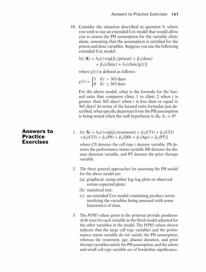
Answers to Practice Exercises 167
10. Consider the situation described in question 9, whereyou wish to use an extended Cox model that would allowyou to assess the PH assumption for the variable clinicalone, assuming that the assumption is satisfied for theprison and dose variables. Suppose you use the followingextended Cox model:
h(t,X) = h0(t) exp[β1(prison) + β2(dose)+ β3(clinic) + δ1(clinic)g (t)]
where g (t) is defined as follows:
g (t) ={
1 if t > 365 days0 if t ≤ 365 days
For the above model, what is the formula for the haz-ard ratio that compares clinic 1 to clinic 2 when t isgreater than 365 days? when t is less than or equal to365 days? In terms of the hazard ratio formulae just de-scribed, what specific departure from the PH assumptionis being tested when the null hypothesis is H0: δ1 = 0?
Answers toPracticeExercises
1. h(t,X) = h0(t) exp[β1(treatment) + β2(CT1) + β3(CT2)+β4(CT3) + β5(PS) + β6(DD) + β7(Age) + β8(PT)]
where CTi denotes the cell type i dummy variable, PS de-notes the performance status variable DD denotes the dis-ease duration variable, and PT denotes the prior therapyvariable.
2. The three general approaches for assessing the PH modelfor the above model are:(a) graphical, using either log–log plots or observed
versus expected plots;(b) statistical test;(c) an extended Cox model containing product terms
involving the variables being assessed with somefunction(s) of time.
3. The P(PH) values given in the printout provide goodness-of-fit tests for each variable in the fitted model adjusted forthe other variables in the model. The P(PH) values shownindicate that the large cell type variables and the perfor-mance status variable do not satisfy the PH assumption,whereas the treatment, age, disease duration, and priortherapy variables satisfy the PH assumption, and the adenoand small cell type variable are of borderline significance.

168 4. Evaluating the Proportional Hazards Assumption
4. A strategy for evaluating the PH assumption using log–logsurvival curves for variables considered one-at-a-time isgiven as follows:
For each variable separately, obtain a plot of obtain log–log Kaplan–Meier curves for the different categories of thatvariable. For the cell type variable, this requires obtaininga plot of four log–log KM curves, one for each cell type.(Note that this is not the same as obtaining four separateplots of two log–log curves, where each plot correspondsto one of the dummy variables used in the model.) Forthe variables PS, DD, and Age, which are interval vari-ables, each variable must be separately categorized intotwo or more groups—say, low versus high values—andKM curves are obtained for each group. For the variablePT, which is a dichotomous variable, two log–log curvesare obtained which compare the “none” versus “some”groups.
For each plot (i.e., one for each variable), those plots thatare noticeably nonparallel indicate variables which do notsatisfy the PH assumption. The remaining variables are as-sumed to satisfy the PH assumption.
5. One strategy for evaluating the PH assumption for eachvariable adjusted for the others is to use adjusted log–logsurvival curves instead of KM curves separately for each ofthe variables in the model. That is, for each variable sepa-rately, a stratified Cox model is fit stratifying on the givenvariable while adjusting for the other variables. Those vari-ables that yield adjusted log–log plots that are noticeablynonparallel are then to be considered as not satisfying thePH assumption. The remaining variables are assumed tosatisfy the PH assumption.
A variation of the above strategy uses adjusted log–logcurves for only those variables not satisfying the PH as-sumption from a one-at-a-time approach, adjusting forthose variables satisfying the PH assumption from the one-at-a-time approach. This second iteration would flag a sub-set of the one-at-a-time flagged variables for further itera-tion. At each new iteration, those variables found to satisfythe assumption get added to the list of variables previouslydetermined to satisfy the assumption.

Answers to Practice Exercises 169
6. For the performance status (PS) variable, observed plotsare obtained by categorizing the variable into strata (say,two strata: low versus high) and then obtaining KM sur-vival plots for each stratum. Expected plots can be ob-tained by fitting a Cox model containing the (continuous)PS variable and then obtaining estimated survival curvesfor values of the performance status (PS) variable that rep-resent summary descriptive statistics for the strata previ-ously identified. For example, if there are two strata, say,high (PS > 50) and low (PS ≤ 50), then the values of PS tobe used could be the mean or median PS score for personsin the high stratum and the mean or median PS score forpersons in the low stratum.
An alternative method for obtaining expected plots in-volves first dichotomizing the PS variable—say, into highand low groups—and then fitting a Cox model contain-ing the dichotomized PS variable instead of the originalcontinuous variable. The expected survival plots for eachgroup are estimated survival curves obtained for each valueof the dichotomized PS variable.
Once observed and expected plots are obtained for eachstratum of the PS variable, they are then compared on thesame graph to determine whether or not correspondingobserved and expected plots are “close.” If it is determinedthat, overall, comparisons for each stratum are close, thenit is concluded that the PH assumption is satisfied for thePH variable. In determining how close is close, the re-searcher should look for noticeably discrepant observedversus expected plots.
7. The log–log plots that compare high versus low PS groups(ignoring other variables) are arguably parallel early infollow-up, and are not comparable later because survivaltimes for the two groups do not overlap after 400 days.These plots do not strongly indicate that the PH assump-tion is violated for the variable PS. This contradicts theconclusion previously obtained for the PS variable usingthe P(PH) results.
8. Drawbacks of the log–log approach are:
� How parallel is parallel?� How to categorize a continuous variable?� How to evaluate several variables simultaneously?
170 4. Evaluating the Proportional Hazards Assumption
Recommendations about problems:
� Look for noticeable nonparallelism; otherwise PH as-sumption is OK.� For continuous variables, use a small number of cat-egories, a meaningful choice of categories, and a rea-sonable balance in sample size for categories.� With several variables, there are two options:
i. Compare log–log curves from combinations of cate-gories.
ii. Adjust for predictors already satisfying PH assump-tion.
9. The observed and expected plots are relatively close forlow and high groups separately, although there is some-what more discrepancy for the high group than for the lowgroup. Deciding how close is close is quite subjective forthese plots. Nevertheless, because there are no major dis-crepancies for either low or high groups, we consider thePH assumption satisfied for this variable.
10. h(t,X) = h0(t) exp[β1(PS) + δ(PS) g (t)]
where g (t) is a function of t, such as g (t) = t, or g (t) =log t, or a heaviside function. The PH assumption is testedusing a 1 df Wald or LR statistic for H0: δ = 0.
11. h(t,X) = h0(t) exp[β1(treatment) + β2(CT1) + β3(CT2)+ β4(CT3) + β5(PS) + β6(DD) + β7(Age) + β8(PT)+ δ1(treatment × g (t)) + δ2(CT1 × g (t)) + δ3(CT2 × g (t))+ δ4(CT3 × g (t)) + δ5(PS × g (t)) + δ6(DD × g (t))+ δ7(Age × g (t)) + δ8(PT × g (t))]
where g (t) is some function of time, such as g (t) = t, org (t) = log t, or a heavyside function. To test the PH as-sumption simultaneously for all variables, the null hypoth-esis is stated as H0: δ1 = δ2 = . . . = δ8 = 0. The test statis-tic is a likelihood-ratio statistic of the form
L R = −2 ln L R − (−2 ln L F )
where R denotes the reduced (PH) model obtained whenall δ’s are 0, and F denotes the full model given above. Un-der H0, the LR statistic is approximately chi-square with8 df.
Answers to Practice Exercises 171
12. The question here is somewhat open-ended, leaving thereader the option to explore additional graphical, GOF, orextended Cox model approaches for evaluating the PH as-sumption for the variables in the model. The conclusionsfrom the GOF statistics provided in question 3 are likely tohold up under further scrutiny, so that a reasonable con-clusion is that cell type and performance status variablesdo not satisfy the PH assumption, with the remaining vari-ables satisfying the assumption.
5 TheStratifiedCoxProcedure
173
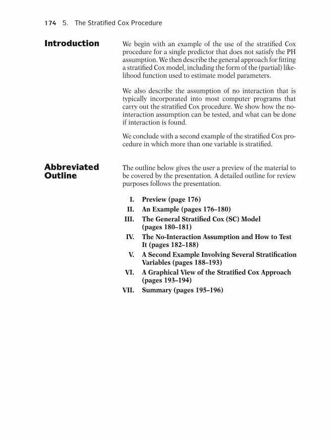
174 5. The Stratified Cox Procedure
Introduction We begin with an example of the use of the stratified Coxprocedure for a single predictor that does not satisfy the PHassumption. We then describe the general approach for fittinga stratified Cox model, including the form of the (partial) like-lihood function used to estimate model parameters.
We also describe the assumption of no interaction that istypically incorporated into most computer programs thatcarry out the stratified Cox procedure. We show how the no-interaction assumption can be tested, and what can be doneif interaction is found.
We conclude with a second example of the stratified Cox pro-cedure in which more than one variable is stratified.
AbbreviatedOutline
The outline below gives the user a preview of the material tobe covered by the presentation. A detailed outline for reviewpurposes follows the presentation.
I. Preview (page 176)II. An Example (pages 176–180)
III. The General Stratified Cox (SC) Model(pages 180–181)
IV. The No-Interaction Assumption and How to TestIt (pages 182–188)
V. A Second Example Involving Several StratificationVariables (pages 188–193)
VI. A Graphical View of the Stratified Cox Approach(pages 193–194)
VII. Summary (pages 195–196)
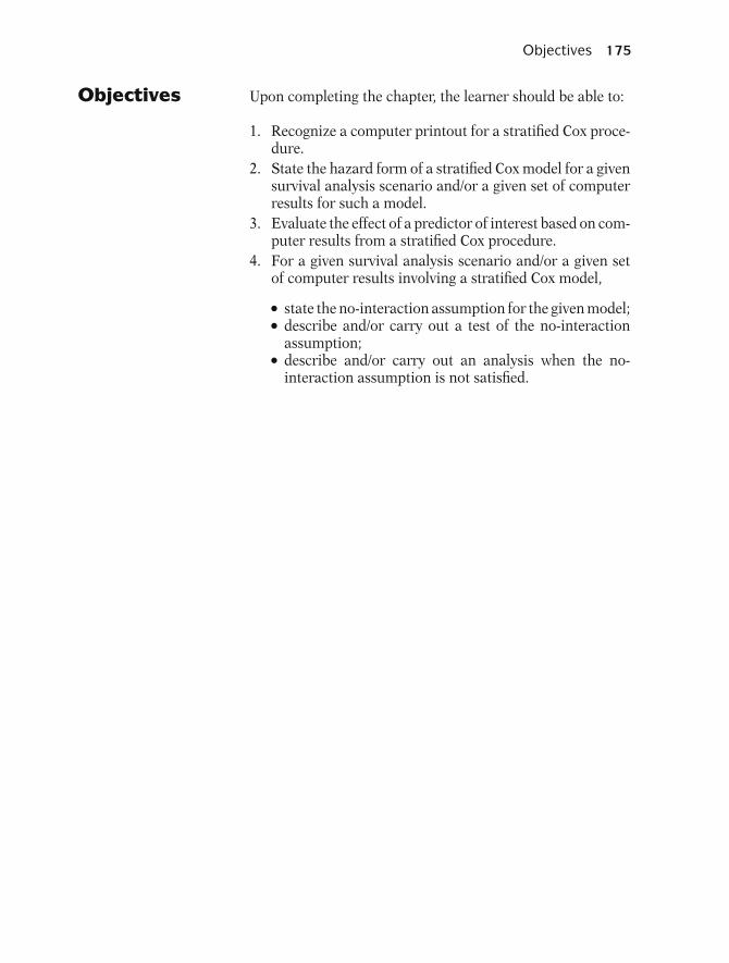
Objectives 175
Objectives Upon completing the chapter, the learner should be able to:
1. Recognize a computer printout for a stratified Cox proce-dure.
2. State the hazard form of a stratified Cox model for a givensurvival analysis scenario and/or a given set of computerresults for such a model.
3. Evaluate the effect of a predictor of interest based on com-puter results from a stratified Cox procedure.
4. For a given survival analysis scenario and/or a given setof computer results involving a stratified Cox model,
� state the no-interaction assumption for the given model;� describe and/or carry out a test of the no-interactionassumption;� describe and/or carry out an analysis when the no-interaction assumption is not satisfied.

176 5. The Stratified Cox Procedure
I. Preview
Stratified Cox model:
� modification of Cox PH model� Stratification of predictor notsatisfying PH� includes predictors satisfyingPH
FOCUS
How stratification iscarried out:• computer results• hazard function• single predictor vs. ≥ 2 predictors• no-interaction vs. interaction
The “stratified Cox model” is a modification of theCox proportional hazards (PH) model that allowsfor control by “stratification” of a predictor thatdoes not satisfy the PH assumption. Predictorsthat are assumed to satisfy the PH assumption areincluded in the model, whereas the predictor be-ing stratified is not included.
In this presentation, we focus on how stratificationis carried out by describing the analysis of com-puter results and the form of the hazard functionfor a stratified Cox model. We first consider strati-fying on a single predictor and then later considerstratifying on two or more predictors. Further, wedistinguish between the use of a “no-interaction”version of the stratified Cox model and an alterna-tive approach that allows interaction.
II. An Example Consider the computer results shown here for aCox PH model containing the three variables, logWBC, treatment group (Rx), and SEX. These re-sults derive from a clinical trial of 42 leukemiapatients, where the response of interest is days inremission.
EXAMPLE
Clinical trial: 42 leukemia patients Response-days in remission
log WBC RxSex
1.5941.3910.263
0.3300.4570.449
0.8280.9350.031
Coef. Std. Err. P(PH)
• log WBC and Rx satisfy PH• Sex does not satisfy PH
(Same conclusions using graphical approaches)
Stratified Cox (SC):
• control for sex (stratified); • simultaneously include log WBC and
Rx in the model
From the printout, the P (PH) values for log WBCand treatment group are nonsignificant. However,the P (PH) value for SEX is significant below the.05 level. These results indicate that log WBCand treatment group satisfy the PH assumption,whereas the SEX variable does not. The same con-clusions regarding the PH assumption about thesevariables would also be made using the graphicalprocedures described earlier.
Because we have a situation where one of thepredictors does not satisfy the PH assumption,we carry out a stratified Cox (SC) procedurefor the analysis. Using SC, we can control forthe SEX variable—which does not satisfy thePH assumption—by stratification while simulta-neously including in the model the log WBC andtreatment variables—which do satisfy the PH as-sumption.

II. An Example 177
EXAMPLE (continued)
STATA OUTPUT USING SC:
Stratified Cox regression Analysis time _t: survt
Stratified Cox regression Analysis time _t: survt
Appendix A illustrates SC procedures using Stata, SAS, and SPSS.
• Log WBC and Rx are included in SC model. • SC model is stratified by SEX.
Effect of Rx adjusted for log WBC and SEX:
• Hazard ratio: 2.537 = e0.931
• Interpretation: Placebo group (Rx = 1) has 2.5 times the hazard as the treatment group (Rx = 0)
95% CI for Rx (1.006, 6.396) indicates considerable variability.
CI formula: exp(0.931 ± 1.96 × 0.472)
Std.Err.Coef.
Haz.Ratio [95% Conf. Interval]
log WBC Rx
p > |z|
1.3900.931
0.3380.472
0.0000.048
4.0162.537
2.0721.006
7.7836.396
No. of subjects = 42 Log likelihood = −57.560 Stratified by sex
Std.Err.Coef.
Haz.Ratio [95% Conf. Interval]
log WBC Rx
p > |z|
1.3900.931
0.3380.472
0.0000.048
4.0162.537
No. of subjects = 42 Log likelihood = −57.560 Stratified by sex
2.0721.006
7.7836.396
Wald test: P = 0.048 (two-tailed), significant at the 0.05 level.
The computer results from a SC procedure areshown here. These results come from the Statapackage. (See the Computer Appendix for runninga SC procedure in Stata, SAS, or SPSS).
The computer results show that the log WBC andRx variables are included in the model listing,whereas the SEX variable is not included; rather,the model stratifies on the SEX variable, as indi-cated at the bottom of the output. Note that theSEX variable is being adjusted by stratification,whereas log WBC is being adjusted by its inclu-sion in the model along with Rx.
In the above output, we have also circled some keyinformation that can be used to assess the effectof the Rx variable adjusted for both log WBC andSEX. In particular, we can see that the hazard ra-tio for the effect of Rx adjusted for log WBC andSEX is given by the value 2.537. This value can beobtained by exponentiating the coefficient 0.931of the Rx variable. The hazard ratio value can beinterpreted to mean that the placebo group (forwhich Rx = 1) has 2.5 times the hazard for goingout of remission as the treatment group (for whichRx = 0).
Also, we can see from the output that a 95% con-fidence interval for the effect of the Rx variable isgiven by the limits 1.006 to 6.396. This is a fairlywide range, thus indicating considerable variabil-ity in the 2.537 hazard ratio point estimate. Notethat these confidence limits can be obtained by ex-ponentiating the quantity 0.931 plus or minus 1.96times the standard error 0.472.
From the above output, a test for the significanceof the Rx variable adjusted for log WBC and SEX isgiven by the Wald statistic P value of 0.048. This isa two-tailed P-value, and the test is just significantat the 0.05 level.

178 5. The Stratified Cox Procedure
LR test: Output for reduced model
EXAMPLE (continued)
Std.Err.Coef.
Haz.Ratio [95% Conf. Interval]
log WBC
p > |z|
1.456 0.320 0.000 4.289 2.291 8.03
No. of subjects = 42 Log likelihood = −59.648 Stratified by sex
SC model for males and females:Females (g = 1):
h1(t,X) = h01(t)exp[β1Rx + β2 log WBC]
Males (g = 2):
h2(t,X) = h02(t)exp[β1Rx + β2 log WBC]
Rx and log WBC in the modelSex not in the model (stratified)
Hazard function for stratified Coxmodel:
hg(t,X) = h0g(t)exp[β1Rx + β2 log WBC]g = 1,2;
g denotes stratum #.
LR and Wald give same conclusion.
Stratified Cox regressionAnalysis time _t: survt
LR = (−2 × −59.648) − (−2 × −57.560) = 119.296 − 115.120 = 4.179 (P < 0.05)
HR for effect of Rx adjusted for log WBCand sex:
eβ1
where β1 is the coefficient of Rx.
An alternative test involves a likelihood ratio (LR)statistic that compares the above model (fullmodel) with a reduced model that does not con-tain the Rx variable. The output for the reducedmodel is shown here. The log-likelihood statisticfor the reduced model is −2 times −59.648,which is to be compared with the log-likelihoodstatistic of −2 times −57.560 for the full model.
The LR statistic is therefore 119.296 minus115.120, which equals 4.179. Under H0, thisstatistic has a chi-square distribution with onedegree of freedom and is significant at the 0.05level. Thus, the LR and Wald tests lead to thesame conclusion.
So far, we have illustrated the results from a strat-ified Cox procedure without actually describingthe model form being used. For the remissiondata example, we now present the hazard func-tion form for the stratified Cox model, as shownhere. This hazard function formula contains asubscript g that indicates the g th stratum.
Thus, in our remission data example, where wehave stratified on SEX, g takes on one of twovalues, so that we have a different baseline hazardfunction for males and females.
Notice that the hazard function formula containsthe variables Rx and log WBC, but does notcontain the variable SEX. SEX is not includedin the model because it doesn’t satisfy the PHassumption. So, instead, the SEX variable iscontrolled by stratification.
Because the variables Rx and log WBC areincluded in the model, we can estimate the effectof each variable adjusted for the other variableand the SEX variable using standard exponentialhazard ratio expressions. For example, the esti-mated hazard ratio for the effect of Rx, adjustedfor log WBC and SEX, is given by e to the β1 “hat,”where β1 is the coefficient of the Rx variable.

II. An Example 179
Cannot estimate HR for SEX variable(SEX doesn’t satisfy PH).
Different baseline hazard functions:
h01(t) for females and h02(t) for males.
No interaction assumption(see Section IV)
Same coefficients β1 and β2 for bothfemale and male models.
EXAMPLE (continued)
Females and males:same β1 and β2⇒ same HR’s, e.g., eβ
1ˆ
Differentbaselines
h01(t) ⇒ Survival curve for femalesh02(t) ⇒ Survival curve for males
{
Estimates of β1 and β2:
Maximize partial likelihood (L),where L = L1 × L2L1 is the likelihood for females derivedfrom h1(t),and L2 is the likelihood for males derivedfrom h2(t).
Nevertheless, because the SEX variable is notincluded in the model, it is not possible to obtaina hazard ratio value for the effect of SEX adjustedfor the other two variables. This is the price to bepaid for stratification on the SEX variable. Notethat a single value for the hazard ratio for SEXis not appropriate if SEX doesn’t satisfy the PHassumption, because the hazard ratio must thenvary with time.
Notice also that the hazard functions for malesand females differ only insofar as they havedifferent baseline hazard functions, namely,h01(t) for females and h02(t) for males. However,the coefficients β1 and β2 are the same for bothfemale and male models.
Because there are different baseline hazardfunctions, the fitted stratified Cox model will yielddifferent estimated survival curves for femalesand males. These curves will be described shortly.
Note, however, that because the coefficients of Rxand log WBC are the same for females and males,estimates of hazard ratios, such as e to the β1“hat,” are the same for both females and males.This feature of the stratified Cox model is calledthe “no-interaction” assumption. It is possibleto evaluate whether this assumption is tenableand to modify the analysis if not tenable. We willdiscuss this assumption further in Section IV.
To obtain estimates of β1 and β2, a (partial)likelihood function (L) is formed from the modeland the data; this function is then maximizedusing computer iteration. The likelihood function(L) for the stratified Cox (SC) model is differentfrom the nonstratified Cox model. For the SCmodel, L is obtained by multiplying togetherlikelihood functions for each stratum. Thus, Lis equal to the product of L1 and L2, where L1and L2 denote the female and male likelihoodfunctions, respectively, which are derived fromtheir respective hazard functions h1(t) and h2(t).
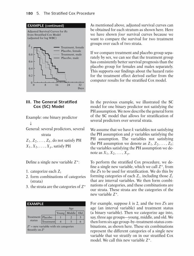
180 5. The Stratified Cox Procedure
EXAMPLE (continued)
Adjusted Survival Curves for Rxfrom Stratified Cox Model(adjusted for log WBC)
1
0.8
0.6
0.4
0.2
00 8 16 24 32
Treatment, female
Treatment, malePlacebo, female
Placebo, male
Days
S
As mentioned above, adjusted survival curves canbe obtained for each stratum as shown here. Herewe have shown four survival curves because wewant to compare the survival for two treatmentgroups over each of two strata.
If we compare treatment and placebo group sepa-rately by sex, we can see that the treatment grouphas consistently better survival prognosis than theplacebo group for females and males separately.This supports our findings about the hazard ratiofor the treatment effect derived earlier from thecomputer results for the stratified Cox model.
III. The General StratifiedCox (SC) Model
In the previous example, we illustrated the SCmodel for one binary predictor not satisfying thePH assumption. We now describe the general formof the SC model that allows for stratification ofseveral predictors over several strata.
Example: one binary predictor↓
General: several predictors, severalstrata
Z1, Z2, . . . , Zk, do not satisfy PHX1, X2, . . . , X p, satisfy PH
We assume that we have k variables not satisfyingthe PH assumption and p variables satisfying thePH assumption. The variables not satisfyingthe PH assumption we denote as Z1, Z2, . . . , Zk;the variables satisfying the PH assumption we de-note as X1, X2, . . . , X p.
Define a single new variable Z ∗:
1. categorize each Z i
2. form combinations of categories(strata)
3. the strata are the categories of Z ∗
To perform the stratified Cox procedure, we de-fine a single new variable, which we call Z ∗, fromthe Z’s to be used for stratification. We do this byforming categories of each Zi , including those Zithat are interval variables. We then form combi-nations of categories, and these combinations areour strata. These strata are the categories of thenew variable Z ∗.
EXAMPLEAge
Young Middle Old
Placebo
Treatment
Treatmentstatus
1 2 3
4 5 6
Z∗ = new variable with six categoriesStratify on Z∗
For example, suppose k is 2, and the two Z’s areage (an interval variable) and treatment status(a binary variable). Then we categorize age into,say, three age groups—young, middle, and old. Wethen form six age group–by–treatment-status com-binations, as shown here. These six combinationsrepresent the different categories of a single newvariable that we stratify on in our stratified Coxmodel. We call this new variable Z ∗.
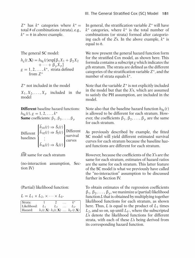
III. The General Stratified Cox (SC) Model 181
Z ∗ has k∗ categories where k∗ =total # of combinations (strata), e.g.,k∗ = 6 in above example.
In general, the stratification variable Z ∗ will havek∗ categories, where k∗ is the total number ofcombinations (or strata) formed after categoriz-ing each of the Z’s. In the above example, k∗ isequal to 6.
The general SC model:
hg (t,X) = h0g (t)exp[β1 X1 + β2 X2+ · · · + βp X p]
g = 1, 2, . . . , k∗, strata definedfrom Z ∗
We now present the general hazard function formfor the stratified Cox model, as shown here. Thisformula contains a subscript g which indicates thegth stratum. The strata are defined as the differentcategories of the stratification variable Z ∗, and thenumber of strata equals k∗.
Z ∗ not included in the model
X1, X2, . . . , X p included in themodel
Note that the variable Z ∗ is not explicitly includedin the model but that the X ’s, which are assumedto satisfy the PH assumption, are included in themodel.
Different baseline hazard functions:h0g (t), g = 1, 2, . . . , k∗
Same coefficients: β1, β2, . . . ,βp
Differentbaselines
⎧⎪⎪⎪⎪⎨⎪⎪⎪⎪⎩h 01(t) ⇒ S1(t)h 02(t) ⇒ S2(t)
...h 0k(t) ⇒ Sk(t)
⎫⎪⎪⎪⎪⎬⎪⎪⎪⎪⎭Differentsurvivalcurves
Note also that the baseline hazard function h0g (t)is allowed to be different for each stratum. How-ever, the coefficients β1,β2, . . . ,βp are the samefor each stratum.
As previously described by example, the fittedSC model will yield different estimated survivalcurves for each stratum because the baseline haz-ard functions are different for each stratum.
HR same for each stratum
(no-interaction assumption, Sec-tion IV)
However, because the coefficients of the X ’s are thesame for each stratum, estimates of hazard ratiosare the same for each stratum. This latter featureof the SC model is what we previously have calledthe “no-interaction” assumption to be discussedfurther in Section IV.
(Partial) likelihood function:
L = L1 × L2, × · · · × Lk∗
Strata: 1 2 . . . k∗
Likelihood: L1 L2 . . . Lk∗
Hazard: h1(t,X) h2(t,X) . . . hk∗ (t,X)
To obtain estimates of the regression coefficientsβ1,β2, . . . ,βp, we maximize a (partial) likelihoodfunction L that is obtained by multiplying togetherlikelihood functions for each stratum, as shownhere. Thus, L is equal to the product of L1 timesL2, and so on, up until Lk∗ , where the subscriptedL’s denote the likelihood functions for differentstrata, with each of these L’s being derived fromits corresponding hazard function.

182 5. The Stratified Cox Procedure
IV. The No-InteractionAssumption and Howto Test It
We previously pointed out that the SC model con-tains regression coefficients, denoted as β’s, thatdo not vary over the strata. We have called thisproperty of the model the “no-interaction assump-tion.” In this section, we explain what this assump-tion means. We also describe how to evaluate theassumption and what to do if the assumption isviolated.
Stratified Cox model
hg (t,X) = h0g (t)exp[β1 X1+β2 X2 + · · · + βp X p]
β coefficients do not vary overstrata (no-interaction assumption)
� how to evaluate� what to do if violated
EXAMPLE
No-interaction SC model:Stratified Cox regressionAnalysis time _t: survt
Std.Err.Coef.
Haz.Ratio [95% Conf. Interval]
log WBC Rx
p > |z|
1.3900.931
0.3380.472
0.0000.048
4.0162.537
2.0721.006
7.7836.396
No. of subjects = 42 Log likelihood = −57.560 Stratified by sex
Interaction by fitting separate models:Cox regression (Females)Analysis time _t: survt
Cox regression (Males)Analysis time _t: survt
Column p-valuename Coeff StErr. 0.95 CI P(PH)HR
4 log WBC
5 Rx
1.639
1.859
0.519 0.002 5.150 1.862 14.242 0.228
0.729 0.011 6.418 1.537 26.790 0.603
Log likelihood = −22.100
Column p-valuename Coeff StErr. 0.95 CI P(PH)HR
4 log WBC
5 Rx
1.170
0.267
0.499 0.019 3.222 1.213 8.562 0.674
0.566 0.637 1.306 0.431 3.959 0.539
No. of subjects = 22 Log likelihood = −33.736
No. of subjects = 20
Which model is more appropriate statistically?
We return to the SC output previously illustrated.Notice that only one set of coefficients, namely,1.390 for log WBC and 0.931 for Rx, are provided,even though there are two strata, one for femalesand one for males. These results assume nointeraction of the sex variable with either logWBC or Rx.
If we allow for interaction, then we wouldexpect to obtain different coefficients for eachof the (SEX) strata. This would happen if we fitseparate hazard models to the female and maledata, with each model containing the log WBCand Rx variables. The computer results fromfitting separate models are shown here.
Notice that the coefficient of log WBC is 1.639 forfemales but is 1.170 for males. Also, the coefficientfor Rx is 1.859 for females but 0.267 for males.These results show different coefficients forfemales than for males, particularly for the Rxvariable.
But are corresponding coefficients statisticallydifferent? That is, which model is more appropri-ate statistically, the no-interaction model or theinteraction model? To answer this question, wemust first look at the hazard function model forthe interaction situation.

IV. The No-Interaction Assumption and How to Test it 183
EXAMPLE (continued)
Interaction model:
No-interaction model:
Alternative interaction model: ( ) hg(t,X) = h0g(t)exp[β1
∗ log WBC + β2
∗Rx + β3∗ (SEX × log WBC) + β4
∗
× (SEX × Rx)]
where SEX = {1 if female 0
h0g(t) are different for g = 1,2 β∗ coefficients do not involve g
Equivalence of models (�) and ( ): g = 1 (females), so that sex = 1:
h1(t,X) = h01(t)exp[β1∗ log WBC + β2
∗ Rx
+ β3∗ (1 × log WBC) + β4
∗ (1 × Rx)]
h2(t,X) = h02(t)exp[β1∗ log WBC + β2
∗ Rx
+β3∗ (0 × log WBC) + β4
∗ (0 × Rx)]
= h01(t)exp[ (β1∗ + β3
∗) log WBC
+ (β2∗ + β4
∗) Rx]
g = 2 (males), so that sex = 0:
= h02(t)exp[ β1∗ log WBC + β2
∗ Rx]
Interaction models in same format:
Females (g = 1): h1 (t,X)(�) = h01(t)exp[β11log WBC + β21Rx]
( ) = h01(t)exp[(β1∗ + β3
∗) log WBC
+ (β2∗ + β4
∗)Rx]
Males (g = 2): h2 (t,X)(�) = h02(t)exp[β12log WBC + β22Rx]
( ) = h02(t)exp[β1∗log WBC + β2
∗ Rx]
if male
(�) hg(t,X)= h0g(t)exp[β1g log WBC + β2gRx]where g = 1 (females), g = 2 (males)
hg(t,X) = h0g(t)exp[β1 log WBC + β2Rx]where g = 1 (females), g = 2 (males)
One way to state the hazard model formula whenthere is interaction is shown here (�). Noticethat each variable in this model has a differentcoefficient for females than for males, as indicatedby the subscript g in the coefficients β1g and β2g .
In contrast, in the no-interaction model, thecoefficient (β1) of log WBC is the same forfemales and for males; also, the coefficient (β2)of Rx is the same for females and for males.
An alternative way to write the interaction modelis shown here (). This alternative form containstwo product terms—SEX × log WBC and SEX ×Rx—as well as the main effects of log WBC andRx. We have coded the SEX so that 1 denotesfemale and 0 denotes male.
In this alternative model, note that although thebaseline hazards h0g (t) are different for each sex,the β∗ coefficients do not involve the subscript gand therefore are the same for each sex.
Nevertheless, this alternative formula () isequivalent to the interaction formula (�) above.We show this by specifying the form that themodel takes for g = 1 (females) and g = 2(males).
Notice that the coefficients of log WBC aredifferent in each formula, namely, (β∗
1 + β∗3) for
females versus β∗1 for males.
Similarly, the coefficients of Rx are different,namely, (β∗
2 + β∗4) for females versus β∗
2 formales.
The preceding formulae indicate that two seem-ingly different formulae for the interactionmodel—(�) versus (), shown earlier—can bewritten in the same format. We show theseformulae here separately for females and males.

184 5. The Stratified Cox Procedure
EXAMPLE (continued)
Females (g = 1): β11 = β1∗ + β3
∗
β21 = β2∗ + β4
∗
(�) ( )
Males (g = 2): β12 = β1∗
β22 = β2∗
(�) ( )
Stratified Cox regression Analysis time _t: survt
logWBC
Rx
Sex× log WBC
Sex× Rx
Std.Err.
0.499
0.566
0.720
0.923
p > |z|
0.019
0.637
0.515
0.084
Haz.Ratio
3.222
1.306
1.598
4.915
[95% Conf. Interval]
1.213 8.562
0.431 3.959
0.390 6.549
0.805 30.003
Coef.
0.469
1.170
0.267
1.592
No. of subjects = 42 Log likelihood = –55.835 Stratified by sex
Females:
Males:
β1∗ + β3
∗ = 1.170 + 0.469 = 1.639
β21 = 1.859
β2∗ + β4
∗ = 0.267 + 1.592 = 1.859Rx
{{
log WBC
log WBC β12 = 1.170 = β1∗
Interaction model:
hg(t,X) = h0g(t)exp[β1∗ log WBC + β2
∗ Rx
+ β3∗ (SEX × log WBC)
+ β4∗ (SEX × Rx)]
β11 = 1.639
Rx β22 = 0.267 = β2∗
Notice that for females, the coefficient β11 inmodel (�) must be equivalent to (β∗
1 + β∗3) in
model () because both models have the same for-mat, and both β11 and (β∗
1 + β∗3) are coefficients
of the same variable, log WBC. Similarly, β21 inmodel (�) is equivalent to (β∗
2 + β∗4) in model ()
because both are coefficients of the same variable,Rx.
For males, it follows in an analogous way,that the coefficient β12 is equivalent to β∗
1, and,similarly, β22 equals β∗
2.
Here we provide computer results obtainedfrom fitting the alternative interaction model ().The estimated regression coefficients β
∗1, β
∗2, β
∗3,
and β∗4, respectively, are circled.
We have shown above that the sums β∗1 + β
∗3 and
β∗2 + β
∗4 are equal to the coefficients β11 and β21,
respectively, in the original interaction model forfemales.
Also, we have shown that β∗1 and β
∗2 are equal
to the coefficients β12 and β22, respectively, inthe original interaction model for the males. Thenumerical equivalences are shown here. Noteagain that the coefficients of log WBC and Rxfor females are different from males, as is to beexpected if sex interacts with each variable.
We have thus seen that the interaction modelcan be written in a format that contains productterms involving the variable being stratified—SEX—being multiplied by each of the predictorsnot being stratified. We show this model involvingproduct terms again here. We will use thismodel to describe a test of the no-interactionassumption.

IV. The No-Interaction Assumption and How to Test it 185
EXAMPLE (continued)
LR = −2 ln LR − (−2 ln LF)R = reduced (no-interaction) modelF = full (interaction) model
LR ~ χ22df under H0: no interaction
(2 df because two product terms testedin interaction model)
Output: –2 log L: 111.670
No interaction (reduced model):
LR = 115.120 – 111.670 = 3.45(P > 0.05 not significant).Thus, the no-interaction model is accep-table.
.
–2 ln LR
–2 ln LF
Output: –2 log L: 115.120
Interaction (full model):
Testing the no-interaction assumption:
The test is a likelihood ratio (LR) test whichcompares log-likelihood statistics for the interac-tion model and the no-interaction model. Thatis, the LR test statistic is of the form −2 ln L Rminus −2 ln L F , where R denotes the reducedmodel, which in this case is the no-interactionmodel, and F denotes the full model, which is theinteraction model.
This LR test statistic has approximately achi-square distribution with 2 degrees of freedomunder the null hypothesis that the no-interactionmodel is correct. The degrees of freedom here is 2because there are two product terms being testedin the interaction model.
The log-likelihood statistic for the reducedmodel comes from the computer output for theno-interaction model and is equal to −2 times−57.560, or 115.120.
The log-likelihood statistic for the full modelcomes from the computer results for the interac-tion model and is equal to −2 times −55.835, or111.670.
The LR statistic is therefore 115.120 minus111.670, which equals 3.45. This value is not sig-nificant at the 0.05 level for 2 degrees of freedom.Thus, it appears that despite the numerical dif-ference between corresponding coefficients in thefemale and male models, there is no statisticallysignificant difference. We can therefore concludefor these data that the no-interaction model isacceptable (at least at the 0.05 level).
Remission data example:� described no-interaction
assumption� evaluated assumption using LRtest� provided interaction model ifneeded
Now, we generalize this process.
Using the remission data example, we havedescribed the no-interaction assumption, haveshown how to evaluate this assumption using alikelihood ratio test, and have provided the formof an interaction model that should be used in casethe no-interaction assumption does not hold. Wenow describe this process more generally for anystratified Cox analysis.
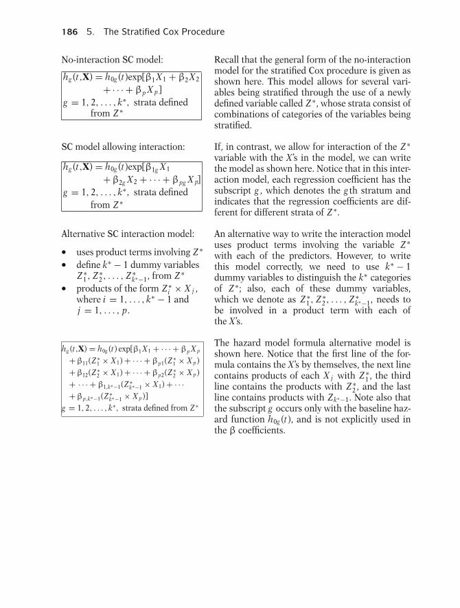
186 5. The Stratified Cox Procedure
No-interaction SC model:
hg (t,X) = h0g (t)exp[β1 X1 + β2 X2
+ · · · + βp X p]g = 1, 2, . . . , k∗, strata defined
from Z ∗
Recall that the general form of the no-interactionmodel for the stratified Cox procedure is given asshown here. This model allows for several vari-ables being stratified through the use of a newlydefined variable called Z ∗, whose strata consist ofcombinations of categories of the variables beingstratified.
SC model allowing interaction:
hg (t,X) = h0g (t)exp[β1g X1
+β2g X2 + · · · + βpg X p]g = 1, 2, . . . , k∗, strata defined
from Z ∗
If, in contrast, we allow for interaction of the Z ∗variable with the X ’s in the model, we can writethe model as shown here. Notice that in this inter-action model, each regression coefficient has thesubscript g , which denotes the g th stratum andindicates that the regression coefficients are dif-ferent for different strata of Z ∗.
Alternative SC interaction model:
� uses product terms involving Z ∗� define k∗ − 1 dummy variables
Z ∗1 , Z ∗
2 , . . . , Z ∗k∗−1, from Z ∗
� products of the form Z ∗i × X j ,
where i = 1, . . . , k∗ − 1 andj = 1, . . . , p.
An alternative way to write the interaction modeluses product terms involving the variable Z ∗with each of the predictors. However, to writethis model correctly, we need to use k∗ − 1dummy variables to distinguish the k∗ categoriesof Z ∗; also, each of these dummy variables,which we denote as Z ∗
1 , Z ∗2 , . . . , Z ∗
k∗−1, needs tobe involved in a product term with each ofthe X ’s.
hg (t,X) = h0g (t) exp[β1 X1 + · · · + βp X p
+β11(Z ∗1 × X1) + · · · + βp1(Z ∗
1 × X p)
+β12(Z ∗2 × X1) + · · · + βp2(Z ∗
2 × X p)
+ · · · + β1,k∗−1(Z ∗k∗−1 × X1) + · · ·
+βp,k∗−1(Z ∗k∗−1 × X p)]
g = 1, 2, . . . , k∗, strata defined from Z ∗
The hazard model formula alternative model isshown here. Notice that the first line of the for-mula contains the X ’s by themselves, the next linecontains products of each X j with Z ∗
1 , the thirdline contains the products with Z ∗
2 , and the lastline contains products with Zk∗−1. Note also thatthe subscript g occurs only with the baseline haz-ard function h0g (t), and is not explicitly used inthe β coefficients.

IV. The No-Interaction Assumption and How to Test it 187
EXAMPLE (Remission Data)
Z∗ = sex, k∗ = 2,
g =1, 2
β1 = β1∗, β2 = β2
∗, β11 = β3∗, and β21 = β4
∗
+ β11(Z∗1 × X1)
= h0g(t)exp[β1∗log WBC
+ β2∗Rx + β3
∗(sex × log WBC)
+ β4∗(sex × Rx)]
Z∗1 = sex(0,1),
X1 = log WBC, X2 = Rx (p = 2)
hg(t,X) = h0g(t)exp[β1X1 + β2X2
+ β21(Z∗1 × X2)]
In our previous example involving the remissiondata, the stratification variable (Z ∗) was the vari-able SEX, and k∗ was equal to 2; thus, we haveonly one dummy variable Z ∗
1 , which uses a (0,1)coding to indicate sex, and we have only ( p equalto) two predictors—X1 equal to log WBC and X2equal to Rx. The interaction model is then writtenin either of the forms shown here.
The latter version of the interaction model is whatwe previously presented for the remission data ex-ample. Because the two versions presented hereare equivalent, it follows that β∗
1 = β1,β2 = β∗2,
β11 = β∗3, and β21 = β∗
4.
We have thus seen that the interaction model canbe written in a format that contains product termsinvolving dummy variables (i.e., Z ∗
i ) for the vari-able being stratified being multiplied by each ofthe predictors (i.e., Xi ) not being stratified. Wewill use this model to describe a test of the no-interaction assumption.
Testing the no-interaction assump-tion:LR = −2 ln L R − (−2 ln L F )R = reduced (no-interaction) modelF = full (interaction) model
contains product terms
H0 :
⎧⎪⎪⎪⎨⎪⎪⎪⎩β11 = · · · = βp1 = 0β12 = · · · = βp2 = 0...β1,k∗−1 = · · · = βp,k∗−1 = 0
The test is a likelihood ratio (LR) test which com-pares log likelihood statistics for the interactionmodel and the no-interaction model. That is, theLR test statistic is of the form −2 ln L R minus−2 ln L F , where R denotes the reduced model,which in this case is the no-interaction model, andF denotes the full model, which is the interactionmodel.
The no-interaction model differs from the inter-action model in that the latter contains additionalproduct terms. Thus, one way to state the null hy-pothesis of no interaction is that the coefficientsof each of these product terms are all zero.
LR ∼ χ2p(k∗−1) df
under H0: no interaction
p(k∗ − 1) gives number of productterms being tested in interactionmodel
The LR test statistic has approximately a chi-square distribution with p(k∗ − 1) degrees of free-dom under the null hypothesis. The degrees offreedom here is p(k∗ − 1) because this value givesthe number of product terms that are being testedin the interaction model.
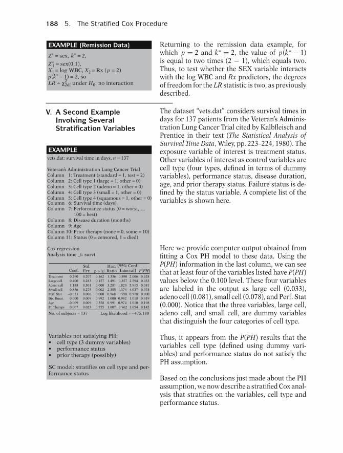
188 5. The Stratified Cox Procedure
EXAMPLE (Remission Data)
Z∗ = sex , k∗ = 2,
Z∗1 = sex(0,1),
X1 = log WBC, X2 = Rx (p = 2) p(k∗ − 1) = 2, so LR ~ χ2
2df under H0: no interaction .
Returning to the remission data example, forwhich p = 2 and k∗ = 2, the value of p(k∗ − 1)is equal to two times (2 − 1), which equals two.Thus, to test whether the SEX variable interactswith the log WBC and Rx predictors, the degreesof freedom for the LR statistic is two, as previouslydescribed.
V. A Second ExampleInvolving SeveralStratification Variables
The dataset “vets.dat” considers survival times indays for 137 patients from the Veteran’s Adminis-tration Lung Cancer Trial cited by Kalbfleisch andPrentice in their text (The Statistical Analysis ofSurvival Time Data, Wiley, pp. 223–224, 1980). Theexposure variable of interest is treatment status.Other variables of interest as control variables arecell type (four types, defined in terms of dummyvariables), performance status, disease duration,age, and prior therapy status. Failure status is de-fined by the status variable. A complete list of thevariables is shown here.
Here we provide computer output obtained fromfitting a Cox PH model to these data. Using theP(PH) information in the last column, we can seethat at least four of the variables listed have P(PH)values below the 0.100 level. These four variablesare labeled in the output as large cell (0.033),adeno cell (0.081), small cell (0.078), and Perf. Stat(0.000). Notice that the three variables, large cell,adeno cell, and small cell, are dummy variablesthat distinguish the four categories of cell type.
Thus, it appears from the P(PH) results that thevariables cell type (defined using dummy vari-ables) and performance status do not satisfy thePH assumption.
Based on the conclusions just made about the PHassumption, we now describe a stratified Cox anal-ysis that stratifies on the variables, cell type andperformance status.
EXAMPLE vets.dat: survival time in days, n = 137
Veteran’s Administration Lung Cancer Trial Column 1: Treatment (standard = 1, test = 2) Column 2: Cell type 1 (large = 1, other = 0) Column 3: Cell type 2 (adeno = 1, other = 0) Column 4: Cell type 3 (small = 1, other = 0) Column 5: Cell type 4 (squamous = 1, other = 0)Column 6: Survival time (days) Column 7: Performance status (0 = worst, ...,
100 = best) Column 8: Disease duration (months) Column 9: Age Column 10: Prior therapy (none = 0, some = 10) Column 11: Status (0 = censored, 1 = died)
Cox regression Analysis time _t: survt
Coef.Std.Err. p > |z|
Haz.Ratio
[95% Conf. Interval] P(PH)
Treatment 0.290 0.207 0.162 1.336 0.890 2.006 0.628Large cell 0.400 0.283 0.157 1.491 0.857 2.594 0.033Adeno cell 1.188 0.301 0.000 3.281 1.820 5.915 0.081Small cell 0.856 0.275 0.002 2.355 1.374 4.037 0.078Perf. Stat –0.033 0.006 0.000 0.968 0.958 0.978 0.000Dis. Durat. 0.000 0.009 0.992 1.000 0.982 1.018 0.919Age –0.009 0.009 0.358 0.991 0.974 1.010 0.198Pr. Therapy 0.007 0.023 0.755 1.007 0.962 1.054 0.145
No. of subjects = 137 Log likelihood = –475.180
Variables not satisfying PH: • cell type (3 dummy variables) • performance status • prior therapy (possibly)
SC model: stratifies on cell type and per-formance status

V. A Second Example Involving Several Stratification Variables 189
EXAMPLE (continued)
Z∗ given by combinations of categories:
Z∗ has k∗= 4 × 2 = 8 categories
• cell type (four categories)• performance status (interval) change
to• PSbin (two categories)
• treatment status• disease duration• age• prior therapy
Four other variables considered as X’s:
Here, we use treatment status and ageas X’s
Stratified Cox regressionAnalysis time _t: survt
Coef.Std.Err. p > |z|
Haz.Ratio
[95% Conf.Interval]
Treatment
Age
0.125 0.208 0.548 1.134 0.753 1.706
– 0.001 0.010 0.897 0.999 0.979 1.019
No. of subjects = 137 Log likelihood = –262.020 Stratified by Z∗
No-interaction model
HR = 1.134 (P = 0.548)
Treatment effect (adjusted for ageand Z∗) is nonsignificant
No-interaction model:
Interaction model:
hg(t,X)= h0g(t)exp[β1 Treatment + β2 Age]g = 1, 2 , . . ., 8 (= # of strata
defined from Z∗)
hg(t,X)= h0g(t)exp[β1g Treatment + β2g Age]g = 1, 2 , . . ., 8
Because we are stratifying on two variables, weneed to form a single new categorical variableZ ∗ whose categories represent combinations ofcategories of the two variables. The cell typevariable has four categories by definition. Theperformance status variable, however, is aninterval variable ranging between 0 for worst to100 for best, so it needs to be categorized. Wecategorize this variable into two groups using acutpoint of 60, and we denote this binary variableas PSbin. Thus, the number of categories for ourZ ∗ variable is 4 × 2, or 8; that is, k∗ = 8.
In addition to the two stratification variables, celltype and performance status, there are four othervariables to be considered as predictors in thestratified Cox model. These are treatment status,disease duration, age, and prior therapy.
For illustrative purposes here, we use onlytreatment status and age as predictors. Theother two variables, disease duration and priortherapy, are considered in exercises following thispresentation.
Here we show computer output from fitting astratified Cox model that stratifies on cell typeand performance status using the eight-categorystratification variable Z ∗. This model also in-cludes treatment and age as predictors. Theseresults consider a no-interaction model, becauseonly one regression coefficient is provided forthe treatment and age predictors. Notice that theestimated hazard ratio is 1.134 for the effect ofthe treatment variable adjusted for age and Z ∗,the latter being adjusted by stratification. Thep-value for this adjusted treatment effect is 0.548,which is highly nonsignificant.
The no-interaction model we have just describedhas the hazard function formula shown here.
To evaluate whether the no-interaction modelis appropriate, we need to define an interactionmodel that allows different regression coeffi-cients for different strata. One way to write thisinteraction model is shown here.
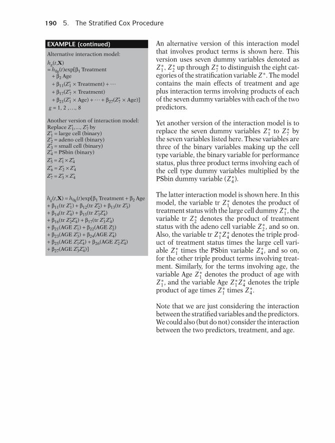
190 5. The Stratified Cox Procedure
EXAMPLE (continued)
Alternative interaction model:
hg(t,X) = h0g(t)exp[β1 Treatment + β2 Age+ β11(tr Z∗
1) + β12(tr Z∗2) + β13(tr Z∗
3)+ β14(tr Z∗
4) + β15(tr Z∗1Z∗
4)+ β16(tr Z∗
2Z∗4) + β17(tr Z∗
3 Z∗4)
+ β21(AGE Z∗1) + β22(AGE Z∗
2)+ β23(AGE Z∗
3) + β24(AGE Z∗4)
+ β25(AGE Z∗1Z∗
4) + β26(AGE Z∗2 Z∗
4)+ β27(AGE Z∗
3Z∗4)]
Another version of interaction model:Replace Z∗
1, ..., Z∗7 by
Z∗1 = large cell (binary)
Z∗2 = adeno cell (binary)
Z∗3 = small cell (binary)
Z∗4 = PSbin (binary)
Z∗5 = Z∗
1 × Z∗4
Z∗6 = Z∗
2 × Z∗4
Z∗7 = Z∗
3 × Z∗4
hg(t,X)= h0g(t)exp[β1 Treatment
+ β2 Age
+ β11(Z∗1 × Treatment) + . . .
+ β17(Z∗7 × Treatment)
+ β21(Z∗1 × Age) + . . . + β27(Z∗
7 × Age)]
g = 1, 2 , . . ., 8
An alternative version of this interaction modelthat involves product terms is shown here. Thisversion uses seven dummy variables denoted asZ ∗
1 , Z ∗2 up through Z ∗
7 to distinguish the eight cat-egories of the stratification variable Z ∗. The modelcontains the main effects of treatment and ageplus interaction terms involving products of eachof the seven dummy variables with each of the twopredictors.
Yet another version of the interaction model is toreplace the seven dummy variables Z ∗
1 to Z ∗7 by
the seven variables listed here. These variables arethree of the binary variables making up the celltype variable, the binary variable for performancestatus, plus three product terms involving each ofthe cell type dummy variables multiplied by thePSbin dummy variable (Z ∗
4).
The latter interaction model is shown here. In thismodel, the variable tr Z ∗
1 denotes the product oftreatment status with the large cell dummy Z ∗
1 , thevariable tr Z ∗
2 denotes the product of treatmentstatus with the adeno cell variable Z ∗
2 , and so on.Also, the variable tr Z ∗
1 Z ∗4 denotes the triple prod-
uct of treatment status times the large cell vari-able Z ∗
1 times the PSbin variable Z ∗4 , and so on,
for the other triple product terms involving treat-ment. Similarly, for the terms involving age, thevariable Age Z ∗
1 denotes the product of age withZ ∗
1 , and the variable Age Z ∗1 Z ∗
4 denotes the tripleproduct of age times Z ∗
1 times Z ∗4 .
Note that we are just considering the interactionbetween the stratified variables and the predictors.We could also (but do not) consider the interactionbetween the two predictors, treatment, and age.
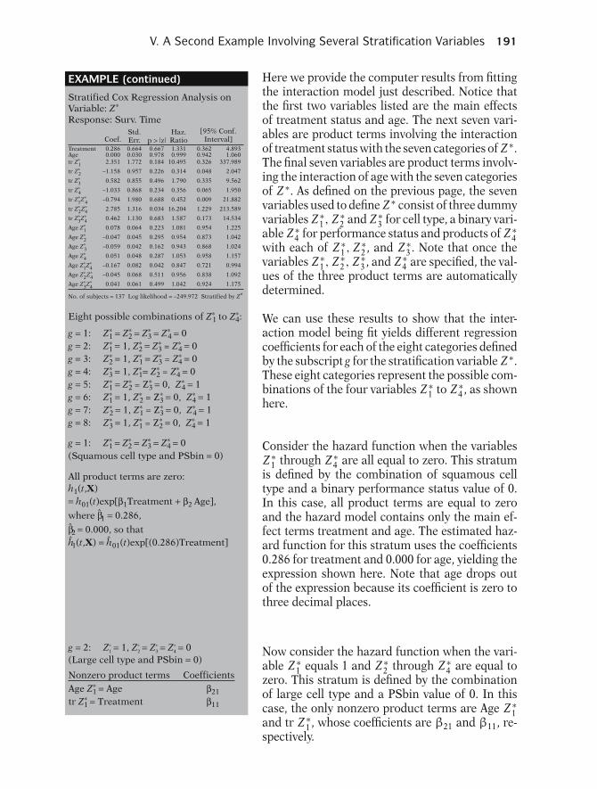
V. A Second Example Involving Several Stratification Variables 191
EXAMPLE (continued)
Coef.Std.Err. p > |z|
Haz.Ratio
[95% Conf. Interval]
Treatment 0.286 0.664 0.667 1.331 0.362 4.893Age 0.000 0.030 0.978 0.999 0.942 1.060tr Z∗
1 2.351 1.772 0.184 10.495 0.326 337.989
tr Z∗2 –1.158 0.957 0.226 0.314 0.048 2.047
tr Z∗3 0.582 0.855 0.496 1.790 0.335 9.562
tr Z∗4 –1.033 0.868 0.234 0.356 0.065 1.950
tr Z∗1Z∗
4 –0.794 1.980 0.688 0.452 0.009 21.882
tr Z∗2Z∗
4 2.785 1.316 0.034 16.204 1.229 213.589
tr Z∗3Z∗
4 0.462 1.130 0.683 1.587 0.173 14.534
Age Z∗1 0.078 0.064 0.223 1.081 0.954 1.225
Age Z∗2 –0.047 0.045 0.295 0.954 0.873 1.042
Age Z∗3 –0.059 0.042 0.162 0.943 0.868 1.024
Age Z∗4 0.051 0.048 0.287 1.053 0.958 1.157
Age Z∗1Z∗
4 –0.167 0.082 0.042 0.847 0.721 0.994
Age Z∗2Z∗
4 –0.045 0.068 0.511 0.956 0.838 1.092
Age Z∗3Z∗
4 0.041 0.061 0.499 1.042 0.924 1.175
Stratified Cox Regression Analysis on Variable: Z∗
Response: Surv. Time
No. of subjects = 137 Log likelihood = –249.972 Stratified by Z∗
Eight possible combinations of Z∗1 to Z∗
4:
g = 1: Z∗1 = Z∗
2 = Z∗3 = Z∗
4 = 0g = 2: Z∗
1 = 1, Z∗2 = Z∗
3 = Z∗4 = 0
g = 3: Z∗2 = 1, Z∗
1 = Z∗3 = Z∗
4 = 0g = 4: Z∗
3 = 1, Z∗1= Z∗
2 = Z∗4 = 0
g = 5: Z∗1 = Z∗
2 = Z∗3 = 0, Z∗
4 = 1g = 6: Z∗
1 = 1, Z∗2 = Z∗
3 = 0, Z∗4 = 1
g = 7: Z∗2 = 1, Z∗
1 = Z∗3 = 0, Z∗
4 = 1g = 8: Z∗
3 = 1, Z∗1 = Z∗
2 = 0, Z∗4 = 1
g = 1: Z∗1 = Z∗
2 = Z∗3 = Z∗
4 = 0(Squamous cell type and PSbin = 0)
All product terms are zero:h1(t,X)= h01(t)exp[β1Treatment + β2 Age],
where β1 = 0.286,
β2 = 0.000, so that h1(t,X) = h01(t)exp[(0.286)Treatment]
g = 2: Z∗1 = 1, Z∗
2 = Z∗3 = Z∗
4 = 0(Large cell type and PSbin = 0)
Nonzero product terms Coefficients
Age Z∗1 = Age β21
tr Z∗1 = Treatment β11
Here we provide the computer results from fittingthe interaction model just described. Notice thatthe first two variables listed are the main effectsof treatment status and age. The next seven vari-ables are product terms involving the interactionof treatment status with the seven categories of Z ∗.The final seven variables are product terms involv-ing the interaction of age with the seven categoriesof Z ∗. As defined on the previous page, the sevenvariables used to define Z ∗ consist of three dummyvariables Z ∗
1 , Z ∗2 and Z ∗
3 for cell type, a binary vari-able Z ∗
4 for performance status and products of Z ∗4
with each of Z ∗1 , Z ∗
2 , and Z ∗3 . Note that once the
variables Z ∗1 , Z ∗
2 , Z ∗3 , and Z ∗
4 are specified, the val-ues of the three product terms are automaticallydetermined.
We can use these results to show that the inter-action model being fit yields different regressioncoefficients for each of the eight categories definedby the subscript g for the stratification variable Z ∗.These eight categories represent the possible com-binations of the four variables Z ∗
1 to Z ∗4 , as shown
here.
Consider the hazard function when the variablesZ ∗
1 through Z ∗4 are all equal to zero. This stratum
is defined by the combination of squamous celltype and a binary performance status value of 0.In this case, all product terms are equal to zeroand the hazard model contains only the main ef-fect terms treatment and age. The estimated haz-ard function for this stratum uses the coefficients0.286 for treatment and 0.000 for age, yielding theexpression shown here. Note that age drops outof the expression because its coefficient is zero tothree decimal places.
Now consider the hazard function when the vari-able Z ∗
1 equals 1 and Z ∗2 through Z ∗
4 are equal tozero. This stratum is defined by the combinationof large cell type and a PSbin value of 0. In thiscase, the only nonzero product terms are Age Z ∗
1and tr Z ∗
1 , whose coefficients are β21 and β11, re-spectively.

192 5. The Stratified Cox Procedure
EXAMPLE (continued)
h2(t,X) = h02(t)exp[(β1 + β11)Treatment+ (β2 + β21) Age]
β1 = 0.286, β2 = 0.000
β11 = 2.351, β21 = 0.078
Hazard functions for interaction model:
g = 1: (Z∗1 = Z∗
2 = Z∗3 = Z∗
4 = 0):h1(t,X) = h01(t)exp[(0.286)Treatment]
g = 2: (Z∗1 = 1, Z∗
2 = Z∗3 = Z∗
4 = 0):h2(t,X) = h02(t)exp[(2.637)Treatment
+ (0.078)Age]g = 3: (Z∗
2 = 1, Z∗1 = Z∗
3 = Z∗4 = 0):
h3(t,X) = h03(t)exp[(−0.872)Treatment
+ (–0.047)Age]g = 4: (Z∗
3 = 1, Z∗1 = Z∗
2 = Z∗4 = 0):
h4(t,X) = h04(t)exp[(0.868)Treatment
+ (−0.059)Age]g = 5: (Z∗
1 = Z∗2 = Z∗
3 = 0, Z∗4 = 1):
h5(t,X) = h05(t)exp[(–0.747)Treatment
+ (0.051)Age]g = 6: (Z∗
1 = 1, Z∗2 = Z∗
3 = 0, Z∗4 = 1):
h6(t,X) = h06(t)exp[(0.810)Treatment
+ (−0.038)Age]g = 7: (Z∗
2 = 1, Z∗1 = Z∗
3 = 0, Z∗4 = 1):
h7(t,X) = h07(t)exp[(0.880)Treatment
+ (−0.041)Age]g = 8: (Z∗
3 = 1, Z∗1 = Z∗
2 = 0, Z∗4 = 1):
h8(t,X) = h08(t)exp[(0.297)Treatment
+ (0.033)Age]
LR test to compare no-interaction modelwith interaction model:
H0: no-interaction model acceptable, i.e.,Treatment: β11 = β12 = . . . = β17 = 0and Age: β21 = β22 = . . . = β27 = 0
14 coefficients ⇒ df = 14
LR = –2 ln LR − (2 ln LF)
F = full (interaction) model
R = reduced (no-interaction) model
The hazard function for this second stratum isshown here. Notice that the coefficients of thetreatment and age variables are (β1 + β11) and(β2 + β21), respectively. The estimated values ofeach of these coefficients are given here.
The corresponding estimated hazard function forthe second stratum (i.e., g = 2) is shown here. Forcomparison, we repeat the estimated hazard func-tion for the first stratum.
The estimated hazard functions for the remain-ing strata are provided here. We leave it up to thereader to verify these formulae. Notice that the co-efficients of treatment are all different in the eightstrata, and the coefficients of age also are all dif-ferent in the eight strata.
We have presented computer results for both theno-interaction and the interaction models. To eval-uate whether the no-interaction assumption is sat-isfied, we need to carry out a likelihood ratio testto compare these two models.
The null hypothesis being tested is that the no-interaction model is acceptable. Equivalently, thisnull hypothesis can be stated by setting the co-efficients of all product terms in the interactionmodel to zero. That is, the seven coefficients ofproduct terms involving treatment and the sevencoefficients of the product terms involving age areset equal to zero as shown here.
Because the null hypothesis involves 14 coeffi-cients, the degrees of freedom of the LR chi-square statistic is 14. The test statistic takes theusual form involving the difference between log-likelihood statistics for the reduced and full mod-els, where the reduced model is the no-interactionmodel and the full model is the interaction model.

VI. A Graphical View of the Stratified Cox Approach 193
EXAMPLE (continued)
LR~χ214df under H0: no interaction
LR = (−2 × –262.020) − (−2 × –249.972)= 524.040 − 499.944 = 24.096
P = 0.045 (significant at 0.05)Conclusion:Reject H0: interaction model ispreferred.
Might use further testing to simplifyinteraction model, e.g., test for sevenproducts involving treatment or test forseven products involving age.
.
Thus, under the null hypothesis, the LR statisticis approximately chi-square with 14 degrees offreedom.
The computer results for the no-interaction andinteraction models give log-likelihood values of524.040 and 499.944, respectively. The differenceis 24.096. A chi-square value of 24.096 with 14 de-grees of freedom yields a p-value of 0.045, so thatthe test gives a significant result at the 0.05 level.This indicates that the no-interaction model is notacceptable and the interaction model is preferred.
Note, however, that it may be possible from fur-ther statistical testing to simplify the interactionmodel to have fewer than 14 product terms. Forexample, one might test for only the seven prod-uct terms involving treatment or only the sevenproduct terms involving age.
VI. A Graphical View of theStratified Cox Approach
a. h(t) = h0(t)exp(β1RX+β2SEX)
ln(− ln S(t)) = ln(− ln S0(t))+β1RX + β2SEX
ln(−lnS(t))
males, RX = 1
males, RX = 0
females, RX = 0
females, RX = 1
t
In this section we examine four log–log survivalplots illustrating the assumptions underlying astratified Cox model with or without interaction.Each of the four models considers two dichoto-mous predictors: treatment (coded RX = 1 forplacebo and RX = 0 for new treatment) and SEX(coded 0 for females and 1 for males). The fourmodels are as follows (see left).
a. h0(t)exp(β1RX + β2SEX). This modelassumes the PH assumption for both RXand SEX and also assumes no interactionbetween RX and SEX. Notice all fourlog–log curves are parallel (PH assumption)and the effect of treatment is the same forfemales and males (no interaction). Theeffect of treatment (controlling for SEX)can be interpreted as the distance betweenthe log–log curves from RX = 1 to RX = 0,for males and for females, separately.

194 5. The Stratified Cox Procedure
b. h(t) = h0(t) exp(β1RX + β2SEX+β3 RX × SEX)
ln(−ln S(t)) = ln(−ln S0(t))+ β1RX+β2SEX+β3RX×SEX
ln(−lnS(t))
males, RX = 1
males, RX = 0
females, RX = 0females, RX = 1
t
c. h(t) = h0g(t)exp(β1RX)(g = 1 for males, g = 0 forfemales)ln(−lnS(t)) = ln(− ln S0g(t))
+ β1RX
ln(−lnS(t))
males, RX = 1males, RX = 0
females, RX = 0
females, RX = 1t
d. h(t) = h0g(t)exp(β1RX+ β2 RX × SEX)
(g = 1 for males, g = 0 forfemales)ln(−ln S(t)) = ln(−ln S0g(t))
+β1RX + β2 RX ×SEX
ln(−lnS(t))
males, RX = 1
males, RX = 0
females, RX = 0
females, RX = 1
t
b. h(t) = h0(t)exp(β1RX + β2SEX + β3RX × SEX). This model assumes the PHassumption for both RX and SEX andallows for interaction between these twovariables. All four log–log curves areparallel (PH assumption) but the effect oftreatment is larger for males than femalesas the distance from RX = 1 to RX = 0 isgreater for males.
c. h(t) = h0g(t)exp(β1RX), where g = 1 formales, g = 0 for females. This is a stratifiedCox model in which the PH assumption isnot assumed for SEX. Notice the curves formales and females are not parallel.However, the curves for RX are parallelwithin each stratum of SEX indicating thatthe PH assumption is satisfied for RX. Thedistance between the log–log curves fromRX = 1 to RX = 0 is the same for malesand females indicating no interactionbetween RX and SEX.
d. h(t) = h0g(t) exp(β1RX + β2RX × SEX),where g = 1 for males, g = 0 for females.This is a stratified Cox model allowing forinteraction of RX and SEX. The curves formales and females are not parallelalthough the PH assumption is satisfied forRX within each stratum of SEX. Thedistance between the log–log curves fromRX = 1 to RX = 0 is greater for males thanfemales indicating interaction between RXand SEX.

VII. Summary 195
VII. Summary We now summarize the most important featuresof the stratified Cox (SC) model described in thispresentation.
The SC model is a modification of the Cox PHmodel to allow for control by “stratification” ofpredictors not satisfying the PH assumption. Vari-ables that are assumed to satisfy the assumptionare included in the model as predictors; the strat-ified variables are not included in the model.
Stratified Cox (SC) model:
� stratification of predictors notsatisfying PH assumption� includes predictors satisfyingPH� does not include stratifiedvariables
Computer Results
Stratified Cox regressionAnalysis time t: survt
Std. Haz. [95% Conf.Coef. Err. p > |z| Ratio Interval]
logWBC 1.390 0.338 0.000 4.016 2.072 7.783RX 0.931 0.472 0.048 2.537 1.006 6.396No. of Log likelihood Stratifiedsubjects = 42 = −57.560 by sex
The computer results for a SC model providesessentially the same type of output as providedfor a Cox PH model without stratification. An ex-ample of SC output using the remission data isshown here. The variables included as predictorsin the model are listed in the first column followedby their estimated coefficients, standard errors,p-values, hazard ratio values, and 95% confidencelimits. Such information cannot be provided forthe variables being stratified, because these lat-ter variables are not explicitly included in themodel.
Hazard function for stratified Coxmodel:
hg (t,X) = h0g (t)exp[β1 X1 + β2 X2
+ · · · + βp X p]g = 1, 2, . . . , k∗, strata defined
from Z ∗
Z ∗ has k∗ categoriesX1, X2, . . . , X p satisfy PH
The general hazard function form for the stratifiedCox model is shown here. This formula containsa subscript g that indicates the gth stratum, wherethe strata are different categories of the stratifica-tion variable Z ∗ and the number of strata equalsk∗. Notice that the baseline hazard functions aredifferent in each stratum.
Stratification variable Z∗:
� identify Z1, Z2, . . . , Zk notsatisfying PH� categorize each Z� form combinations of categories(strata)� each combination is a stratumof Z ∗
The variable Z ∗ is defined by first identifying theZi variables not satisfying the PH assumption. Wethen categorize each Z and form combinations ofcategories of each of the Z’s. Each combinationrepresents a different stratum making up the vari-able Z ∗.

196 5. The Stratified Cox Procedure
No-interaction model:Same coefficients β1,β2, . . . ,βpfor each g, i.e., Z ∗ does not interactwith the X ’s.
The above model is designated as a “no-interaction” model because the β’s in the modelare the same for each subscript g. The no-interaction assumption means that the variablesbeing stratified are assumed not to interact withthe X ’s in the model.
Differentbaselines
⎧⎪⎪⎪⎨⎪⎪⎪⎩h01(t) ⇒ S1(t)h02(t) ⇒ S2(t)
...h0k(t) ⇒ Sk∗ (t)
⎫⎪⎪⎪⎬⎪⎪⎪⎭Differentsurvivalcurves
For the no-interaction model, the fitted SC modelwill yield different estimated survival curves foreach stratum because the baseline hazard func-tions are different for each stratum.
HR same for each stratum However, because the coefficients of the X ’s are thesame for each stratum, estimates of hazard ratiosare the same for each stratum.
(Partial) likelihood function:
L = L1 × L2 × · · · × Lk∗
Regression coefficients in the SC model are esti-mated by maximizing a partial likelihood functionthat is obtained by multiplying likelihood func-tions for each stratum.
Stratified Cox model allowing interaction:
hg (t,X) = h0 g (t) exp[β1g X1 + β2g X2
+ · · · + βpg X p]
g = 1, 2, . . . , k∗, strata defined from Z ∗.
In order to evaluate the no-interaction assump-tion, we must define an interaction model for com-parison. One version of the interaction model isshown here. This version shows regression coeffi-cients with different subscripts in different strata;that is, each β coefficient has a subscript g.
Alternative stratified Cox interac-tion model:
� uses product terms involving Z ∗� define k∗ − 1 dummy variables
from Z ∗� products of the form Z ∗
i × X j
An alternative way to write the interaction modeluses product terms involving the Z ∗ variable witheach predictor. This model uses k∗−1 dummy vari-ables to distinguish the k∗ categories of Z ∗. Eachof these dummy variables is included as a productterm with each of the X ’s.
Testing the no-interaction assump-tion:
LR = −2 ln L R − (2 ln L F )R = reduced (no-interaction) modelF = full (interaction) model
contains product termsLR∼χ2
p(k∗−1)df under H0: nointeraction
To evaluate the no-interaction assumption, we canperform a likelihood ratio test that compares the(reduced) no-interaction model to the (full) inter-action model. The null hypothesis is that the no-interaction assumption is satisfied. The test statis-tic is given by the difference between the log-likelihood statistics for the no-interaction and in-teraction models. This statistic is approximatelychi-square under the null hypothesis. The degreesof freedom is p(k∗−1) where p denotes the num-ber of X ’s and k∗ is the number of categories mak-ing up Z ∗.

VII. Summary 197
PRESENTATION COMPLETE!
Chapters This presentation is now complete. We suggestthat the reader review this presentation using thedetailed outline that follows. Then answer thepractice exercises and the test that follow.
The next Chapter (6) is entitled “Extension of theCox PH Model for Time-Dependent Variables.”There we show how an “extended” Cox modelcan be used as an alternative to the stratified Coxmodel when one or more predictors do not satisfythe PH assumption. We also discuss more gener-ally what is a time-dependent variable, and showhow such a variable can be evaluated using an ex-tended Cox model.
1. Introduction to SurvivalAnalysis
2. Kaplan–Meier Survival Curvesand the Log–Rank Test
3. The Cox Proportional HazardsModel and Its Characteristics
4. Evaluating the ProportionalHazards Assumption
√5.
��
��The Stratified Cox Procedure
Next:
6. Extension of the CoxProportional Hazards Model forTime-Dependent Variables

198 5. The Stratified Cox Procedure
DetailedOutline
I. Preview (page 176)A. Focus on how stratified Cox (SC) procedure is
carried out:� analysis of computer results from SCprocedure;� hazard function for SC model;� stratifying on a single predictor versus two ormore predictors;� no-interaction versus interaction models.
II. An Example (pages 176–180)A. Cox PH results for remission data yield
P (PH) = 0.031 for SEX.B. SC model used: control for SEX (stratified);
include log WBC and Rx in model.C. Analysis of Rx effect from stratified Cox
results:HR = 2.537; 95% CI: (1.006,6.396); LR andWald tests: P < 0.05.
D. Hazard model: hg (t, X) =h0g(t) exp[β1 log WBC + β2 Rx], g = 1,2� different baseline hazard functions and
survival curves for females and males;� same coefficients β1 and β2 for both femalesand males (no-interaction assumption);� obtain estimates by maximizing partiallikelihood L = L1 × L2.
E. Graph of four adjusted survival curves for Rx(adjusted for log WBC).
III. The General Stratified Cox (SC) Model(pages 180–181)A. hg (t,X) = h0g (t) exp [β1 X1 +β2 X2 + · · · +βp X p],
g = 1, 2, · · · , k∗ ,
where the strata are defined from the stratificationvariable Z ∗.
B. Z ∗ defined from Z1, Z2, . . . , Zk variables that donot satisfy PH:� categorize each Zi� form combinations of categories� each combination is a stratum of Z ∗
C. Different baseline hazard functions and survivalcurves for each stratum.
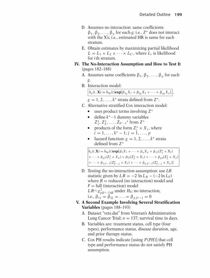
Detailed Outline 199
D. Assumes no interaction: same coefficientsβ1,β2, . . . ,βp for each g; i.e., Z ∗ does not interactwith the X’s; i.e., estimated HR is same for eachstratum.
E. Obtain estimates by maximizing partial likelihoodL = L1 × L2 × · · · × Lk∗ , where Li is likelihoodfor ith stratum.
IV. The No-Interaction Assumption and How to Test It(pages 182–188)A. Assumes same coefficients β1,β2, . . . ,βp for each
g.B. Interaction model:
hg (t, X) = h0g (t)exp[β1g X1 + β2g X2 + · · · + βpg X p] ,
g = 1, 2, . . . , k∗ strata defined from Z ∗.C. Alternative stratified Cox interaction model:� uses product terms involving Z ∗
� define k∗−1 dummy variablesZ ∗
1 , Z ∗2 , . . . , Zk∗−1
∗ from Z ∗� products of the form Z ∗
i × X j , wherei = 1, . . . , k∗ − 1; j = 1, . . . , p� hazard function: g = 1, 2, . . . , k∗ stratadefined from Z ∗
hg (t,X) = h0g (t)exp[β1 X1 + · · · + βp X p + β11(Z ∗1 × X1)
+ · · · + βp1(Z ∗1 × X p) + β12(Z ∗
2 × X1) + · · · + βp2(Z ∗2 × X p)
+ · · · + β1,k∗−1(Z ∗k∗−1 × X1) + · · · + βp,k∗−1(Z ∗
k∗−1 × X p)]
D. Testing the no-interaction assumption: use LRstatistic given by L R = −2 ln L R − (−2 ln LF)where R = reduced (no interaction) model andF = full (interaction) modelL R∼χ2
p(k∗−1)df under H0: no interaction,i.e., β11 = β21 = . . . = βp,k∗−1 = 0
V. A Second Example Involving Several StratificationVariables (pages 188–193)A. Dataset “vets.dat” from Veteran’s Administration
Lung Cancer Trial; n = 137; survival time in days.B. Variables are: treatment status, cell type (four
types), performance status, disease duration, age,and prior therapy status.
C. Cox PH results indicate [using P (PH)] that celltype and performance status do not satisfy PHassumption.
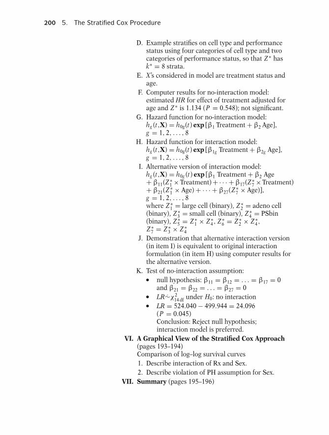
200 5. The Stratified Cox Procedure
D. Example stratifies on cell type and performancestatus using four categories of cell type and twocategories of performance status, so that Z ∗ hask∗ = 8 strata.
E. X ’s considered in model are treatment status andage.
F. Computer results for no-interaction model:estimated HR for effect of treatment adjusted forage and Z ∗ is 1.134 (P = 0.548); not significant.
G. Hazard function for no-interaction model:hg (t,X) = h0g(t) exp [β1 Treatment + β2 Age],g = 1, 2, . . . , 8
H. Hazard function for interaction model:hg (t,X) = h0g(t) exp [β1g Treatment + β2g Age],g = 1, 2, . . . , 8
I. Alternative version of interaction model:hg (t,X) = h0g (t) exp [β1 Treatment + β2 Age+ β11(Z ∗
1 × Treatment) + · · · + β17(Z ∗7 × Treatment)
+ β21(Z ∗1 × Age) + · · · + β27(Z ∗
7 × Age)],g = 1, 2, . . . , 8where Z ∗
1 = large cell (binary), Z ∗2 = adeno cell
(binary), Z ∗3 = small cell (binary), Z ∗
4 = PSbin(binary), Z ∗
5 = Z ∗1 × Z ∗
4 , Z ∗6 = Z ∗
2 × Z ∗4 ,
Z ∗7 = Z ∗
3 × Z ∗4
J. Demonstration that alternative interaction version(in item I) is equivalent to original interactionformulation (in item H) using computer results forthe alternative version.
K. Test of no-interaction assumption:� null hypothesis: β11 = β12 = . . . = β17 = 0and β21 = β22 = . . . = β27 = 0� LR∼χ2
14 df under H0: no interaction� LR = 524.040 − 499.944 = 24.096(P = 0.045)Conclusion: Reject null hypothesis;interaction model is preferred.
VI. A Graphical View of the Stratified Cox Approach(pages 193–194)Comparison of log–log survival curves1. Describe interaction of Rx and Sex.2. Describe violation of PH assumption for Sex.
VII. Summary (pages 195–196)
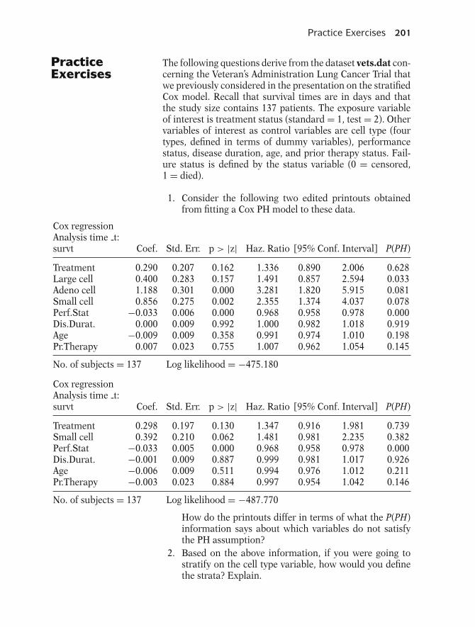
Practice Exercises 201
PracticeExercises
The following questions derive from the dataset vets.dat con-cerning the Veteran’s Administration Lung Cancer Trial thatwe previously considered in the presentation on the stratifiedCox model. Recall that survival times are in days and thatthe study size contains 137 patients. The exposure variableof interest is treatment status (standard = 1, test = 2). Othervariables of interest as control variables are cell type (fourtypes, defined in terms of dummy variables), performancestatus, disease duration, age, and prior therapy status. Fail-ure status is defined by the status variable (0 = censored,1 = died).
1. Consider the following two edited printouts obtainedfrom fitting a Cox PH model to these data.
Cox regressionAnalysis time t:survt Coef. Std. Err. p > |z| Haz. Ratio [95% Conf. Interval] P(PH)
Treatment 0.290 0.207 0.162 1.336 0.890 2.006 0.628Large cell 0.400 0.283 0.157 1.491 0.857 2.594 0.033Adeno cell 1.188 0.301 0.000 3.281 1.820 5.915 0.081Small cell 0.856 0.275 0.002 2.355 1.374 4.037 0.078Perf.Stat −0.033 0.006 0.000 0.968 0.958 0.978 0.000Dis.Durat. 0.000 0.009 0.992 1.000 0.982 1.018 0.919Age −0.009 0.009 0.358 0.991 0.974 1.010 0.198Pr.Therapy 0.007 0.023 0.755 1.007 0.962 1.054 0.145
No. of subjects = 137 Log likelihood = −475.180
Cox regressionAnalysis time t:survt Coef. Std. Err. p > |z| Haz. Ratio [95% Conf. Interval] P(PH)
Treatment 0.298 0.197 0.130 1.347 0.916 1.981 0.739Small cell 0.392 0.210 0.062 1.481 0.981 2.235 0.382Perf.Stat −0.033 0.005 0.000 0.968 0.958 0.978 0.000Dis.Durat. −0.001 0.009 0.887 0.999 0.981 1.017 0.926Age −0.006 0.009 0.511 0.994 0.976 1.012 0.211Pr.Therapy −0.003 0.023 0.884 0.997 0.954 1.042 0.146
No. of subjects = 137 Log likelihood = −487.770
How do the printouts differ in terms of what the P(PH)information says about which variables do not satisfythe PH assumption?
2. Based on the above information, if you were going tostratify on the cell type variable, how would you definethe strata? Explain.
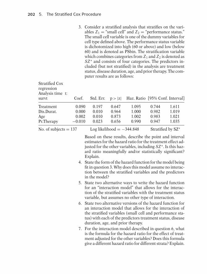
202 5. The Stratified Cox Procedure
3. Consider a stratified analysis that stratifies on the vari-ables Z1 = “small cell” and Z2 = “performance status.”The small cell variable is one of the dummy variables forcell type defined above. The performance status variableis dichotomized into high (60 or above) and low (below60) and is denoted as PSbin. The stratification variablewhich combines categories from Z1 and Z2 is denoted asSZ ∗ and consists of four categories. The predictors in-cluded (but not stratified) in the analysis are treatmentstatus, disease duration, age, and prior therapy. The com-puter results are as follows:
Stratified CoxregressionAnalysis time t:survt Coef. Std. Err. p > |z| Haz. Ratio [95% Conf. Interval]
Treatment 0.090 0.197 0.647 1.095 0.744 1.611Dis.Durat. 0.000 0.010 0.964 1.000 0.982 1.019Age 0.002 0.010 0.873 1.002 0.983 1.021Pr.Therapy −0.010 0.023 0.656 0.990 0.947 1.035
No. of subjects = 137 Log likelihood = −344.848 Stratified by SZ∗
Based on these results, describe the point and intervalestimates for the hazard ratio for the treatment effect ad-justed for the other variables, including SZ ∗. Is this haz-ard ratio meaningfully and/or statistically significant?Explain.
4. State the form of the hazard function for the model beingfit in question 3. Why does this model assume no interac-tion between the stratified variables and the predictorsin the model?
5. State two alternative ways to write the hazard functionfor an “interaction model” that allows for the interac-tion of the stratified variables with the treatment statusvariable, but assumes no other type of interaction.
6. State two alternative versions of the hazard function foran interaction model that allows for the interaction ofthe stratified variables (small cell and performance sta-tus) with each of the predictors treatment status, diseaseduration, age, and prior therapy.
7. For the interaction model described in question 6, whatis the formula for the hazard ratio for the effect of treat-ment adjusted for the other variables? Does this formulagive a different hazard ratio for different strata? Explain.
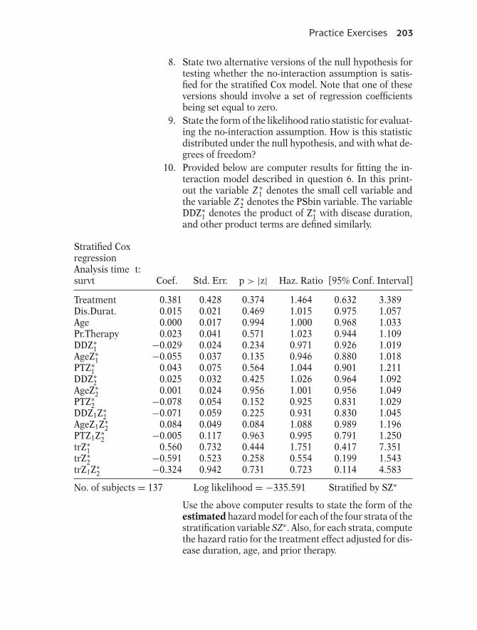
Practice Exercises 203
8. State two alternative versions of the null hypothesis fortesting whether the no-interaction assumption is satis-fied for the stratified Cox model. Note that one of theseversions should involve a set of regression coefficientsbeing set equal to zero.
9. State the form of the likelihood ratio statistic for evaluat-ing the no-interaction assumption. How is this statisticdistributed under the null hypothesis, and with what de-grees of freedom?
10. Provided below are computer results for fitting the in-teraction model described in question 6. In this print-out the variable Z ∗
1 denotes the small cell variable andthe variable Z ∗
2 denotes the PSbin variable. The variableDDZ∗
1 denotes the product of Z∗1 with disease duration,
and other product terms are defined similarly.
Stratified CoxregressionAnalysis time t:survt Coef. Std. Err. p > |z| Haz. Ratio [95% Conf. Interval]
Treatment 0.381 0.428 0.374 1.464 0.632 3.389Dis.Durat. 0.015 0.021 0.469 1.015 0.975 1.057Age 0.000 0.017 0.994 1.000 0.968 1.033Pr.Therapy 0.023 0.041 0.571 1.023 0.944 1.109DDZ∗
1 −0.029 0.024 0.234 0.971 0.926 1.019AgeZ∗
1 −0.055 0.037 0.135 0.946 0.880 1.018PTZ∗
1 0.043 0.075 0.564 1.044 0.901 1.211DDZ∗
2 0.025 0.032 0.425 1.026 0.964 1.092AgeZ∗
2 0.001 0.024 0.956 1.001 0.956 1.049PTZ∗
2 −0.078 0.054 0.152 0.925 0.831 1.029DDZ1Z∗
2 −0.071 0.059 0.225 0.931 0.830 1.045AgeZ1Z∗
2 0.084 0.049 0.084 1.088 0.989 1.196PTZ1Z∗
2 −0.005 0.117 0.963 0.995 0.791 1.250trZ∗
1 0.560 0.732 0.444 1.751 0.417 7.351trZ∗
2 −0.591 0.523 0.258 0.554 0.199 1.543trZ1Z∗
2 −0.324 0.942 0.731 0.723 0.114 4.583
No. of subjects = 137 Log likelihood = −335.591 Stratified by SZ∗
Use the above computer results to state the form of theestimated hazard model for each of the four strata of thestratification variable SZ∗. Also, for each strata, computethe hazard ratio for the treatment effect adjusted for dis-ease duration, age, and prior therapy.

204 5. The Stratified Cox Procedure
11. Carry out the likelihood ratio test to evaluate the no-interaction model described in question 4. In carryingout this test, make sure to state the null hypothesis interms of regression coefficients being set equal to zero inthe interaction model fitted in question 10. Also, deter-mine the p-value for this test and state your conclusionsabout significance as well as which model you prefer, theno-interaction model or the interaction model.
12. The adjusted log–log survival curves for each of the fourstrata defined by the stratification variable SZ ∗ (adjustedfor treatment status, disease duration, age, and priortherapy) are presented below.
6
4
2
0
0 200 400 600 800 Days−2
Adjusted log–log survival curves by SZ∗S adj ∗∗∗
Using this graph, what can you conclude about whetherthe PH assumption is satisfied for the variables, smallcell type and PSbin?
13. Comment on what you think can be learned by graphingadjusted survival curves that compare the two treatmentgroups for each of the four strata of SZ ∗.
Test The following questions consider a dataset from a studyby Caplehorn et al. (“Methadone Dosage and Retention ofPatients in Maintenance Treatment,” Med. J. Aust., 1991).These data comprise the times in days spent by heroin addictsfrom entry to departure from one of two methadone clinics.Two other covariates, namely, prison record and maximummethadone dose, are believed to affect the survival times. Thedataset name is addicts.dat. A listing of the variables is givenbelow:
Column 1: Subject IDColumn 2: Clinic (1 or 2)

Test 205
Column 3: Survival status (0 = censored, 1 = departedfrom clinic)
Column 4: Survival time in daysColumn 5: Prison record (0 = none, 1 = any)Column 6: Maximum methadone dose (mg/day)
1. The following edited printout was obtained from fitting aCox PH model to these data:
Cox regressionAnalysis time t:survt Coef. Std. Err. p > |z| Haz. Ratio [95% Conf. Interval] P(PH)
clinic −1.009 0.215 0.000 0.365 0.239 0.556 0.001prison 0.327 0.167 0.051 1.386 0.999 1.924 0.332dose −0.035 0.006 0.000 0.965 0.953 0.977 0.341
No. of subjects = 238 Log likelihood = −673.403
Based on the P(PH) information in the above printout, itappears that clinic does not satisfy the PH assumption;this conclusion is also supported by comparing log–logcurves for the two clinics and noticing strong nonparal-lelism. What might we learn from fitting a stratified Cox(SC) model stratifying on the clinic variable? What is adrawback to using a SC procedure that stratifies on theclinic variable?
2. The following printout was obtained from fitting a SC PHmodel to these data, where the variable being stratified isclinic:
Stratified CoxregressionAnalysis time t:survt Coef. Std. Err. p > |z| Haz. Ratio [95% Conf. Interval]
Prison 0.389 0.169 0.021 1.475 1.059 2.054Dose −0.035 0.006 0.000 0.965 0.953 0.978
No. of subjects = 238 Log likelihood = −597.714 Stratified by clinic
Using the above fitted model, we can obtain the adjustedcurves below that compare the adjusted survival probabil-ities for each clinic (i.e., stratified by clinic) adjusted forthe variables, prison and maximum methadone dose.
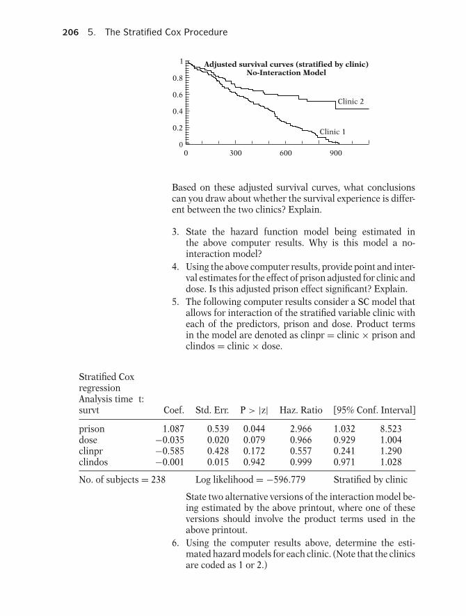
206 5. The Stratified Cox Procedure
0.2
0.4
0.6
0.8
1
0 300 600 9000
Adjusted survival curves (stratified by clinic)No-Interaction Model
Clinic 2
Clinic 1
Based on these adjusted survival curves, what conclusionscan you draw about whether the survival experience is differ-ent between the two clinics? Explain.
3. State the hazard function model being estimated inthe above computer results. Why is this model a no-interaction model?
4. Using the above computer results, provide point and inter-val estimates for the effect of prison adjusted for clinic anddose. Is this adjusted prison effect significant? Explain.
5. The following computer results consider a SC model thatallows for interaction of the stratified variable clinic witheach of the predictors, prison and dose. Product termsin the model are denoted as clinpr = clinic × prison andclindos = clinic × dose.
Stratified CoxregressionAnalysis time t:survt Coef. Std. Err. P > |z| Haz. Ratio [95% Conf. Interval]
prison 1.087 0.539 0.044 2.966 1.032 8.523dose −0.035 0.020 0.079 0.966 0.929 1.004clinpr −0.585 0.428 0.172 0.557 0.241 1.290clindos −0.001 0.015 0.942 0.999 0.971 1.028
No. of subjects = 238 Log likelihood = −596.779 Stratified by clinic
State two alternative versions of the interaction model be-ing estimated by the above printout, where one of theseversions should involve the product terms used in theabove printout.
6. Using the computer results above, determine the esti-mated hazard models for each clinic. (Note that the clinicsare coded as 1 or 2.)

Answers to Practice Exercises 207
7. Below are the adjusted survival curves for each clinicbased on the interaction model results above. Thesecurves are adjusted for the prison and dose variables.
0.2
0.4
0.6
0.8
1
0 300 600 900
0
Adjusted survival curves (stratified by clinic)Interaction Model
Clinic 2
Clinic 1
Compare the survival curves by clinic obtained for theinteraction model with the corresponding curves previ-ously shown for the no-interaction model. Do both curvesindicate the similar conclusions about the clinic effect?Explain.
8. Carry out a likelihood ratio test to determine whether theno-interaction model is appropriate. In doing so, make useof the computer information described above, state thenull hypothesis, state the form of the likelihood statisticand its distribution under the null hypothesis, and com-pute the value of the likelihood statistic and evaluate itssignificance. What are your conclusions?
Answers toPracticeExercises
1. The first printout indicates that the variables large cell,adeno cell, small cell, and performance status do not sat-isfy the PH assumption at the 0.10 level. The second print-out considers a different model that does not contain thelarge cell and adeno cell variables. This latter printout in-dicates that small cell satisfies the PH assumption, in con-trast to the first printout. The performance status variable,however, does not satisfy the PH assumption as in the firstprintout.
2. The cell type variable is defined to have four categories,as represented by the three dummy variables in the firstprintout. The “small cell” variable dichotomizes the celltype variable into the categories small cell type versus therest. From the second printout, the small cell variable doesnot appear by itself to violate the PH assumption. This re-sult conflicts with the results of the first printout, for whichthe cell type variable considered in four categories does not

208 5. The Stratified Cox Procedure
satisfy the PH assumption at the 0.10 level of significance.We therefore think it is more appropriate to use a SC pro-cedure only if four strata are to be used. A drawback tousing four strata, however, is that the number of survivalcurves to be plotted is larger than for two strata; conse-quently, a large number of curves is more difficult to in-terpret graphically than when there are only two curves.Thus, for convenience of interpretation, we may chooseto dichotomize the cell type variable instead of consider-ing four strata. We may also consider dichotomies otherthan those defined by the small cell variable. For instance,we might consider dichotomizing on either the adeno orlarge cell variables instead of the small cell variable. Al-ternatively, we may combine categories so as to compare,say, large and adeno cell types with small and squamoustypes. However, a decision to combine categories shouldnot be just a statistical decision, but should also be basedon biologic considerations.
3. HRadj = 1.095, 95% CI: (0.744,1.611), two-tailed P-value is0.647, not significant. The estimated hazard ratio for treat-ment is neither meaningfully or statistically significant.The point estimate is essentially 1, which says that there isno meaningful effect of treatment adjusted for the predic-tors in the model and for the stratified predictor SZ ∗.
4. hg (t,X) = h0g(t)exp[β1Treatment + β2DD + β3 Age+ β4PT], g = 1, . . . , 4, where the strata are defined fromthe stratification variable SZ ∗, DD = disease duration,and PT = prior therapy. This model assumes no interac-tion because the coefficient of each predictor in the modelis not subscripted by g, i.e., the regression coefficients arethe same for each stratum.
5. Version 1: hg (t, X) = h0g (t)exp[β1g Treatment + β2 DD+ β3 Age + β4 PT], g = 1, . . . , 4.
Version 2: hg (t,X) = h0g(t)exp[β1 Treatment + β2 DD+ β3 Age + β4 PT + β5(Z ∗
1 × Treatment)+ β6(Z ∗
2 × Treatment) + β7(Z ∗1 × Z ∗
2 × Treatment)],where Z ∗
1 = small cell type (0, 1), Z ∗2 = PSbin (0, 1),
and g = 1, . . . , 4.
Answers to Practice Exercises 209
6. Version 1: hg (t,X) = h0g (t)exp[β1g Treatment + β2g DD+ β3g Age + β4g PT], g = 1, . . . , 4.
Version 2: hg (t,X) = h0g (t)exp[β1 Treatment + β2 DD
+ β3 Age + B4 PT + β5(Z ∗1 × Treatment) + β6(Z ∗
1 × DD)
+ β7(Z ∗1 × Age) + β8(Z ∗
1 × PT) + β9(Z ∗2 × Treatment)
+ β10(Z ∗2 × DD) + β11(Z ∗
2 × Age) + β12(Z ∗2 × PT)
+ β13(Z ∗1 × Z ∗
2 × Treatment) + β14(Z ∗1 × Z ∗
2 × DD)
+ β15(Z ∗1 × Z ∗
2 × Age) + β16(Z ∗1 × Z ∗
2 × PT)],
g = 1, . . . , 4.
7. HRg = exp(β1g ), using version 1 model form. Yes, this for-mula gives different hazard ratios for different strata be-cause the value of the hazard ratio changes with the sub-script g.
8. H0: No interaction assumption is satisfied.
H0: β11 = β12 = β13 = β14, β21 = β22 = β23 = β24,
β31 = β32 = β33 = β34, β41 = β42 = β43 = β44from version 1.
H0: β5 = β6 = β7 = β8 = β9 = β10 = β11 = β12= β13 = β14 = β15 = β16 = 0 from version 2.
9. LR = −2 ln L R − (−2 ln L F ), where R denotes the reduced(no-interaction) model and F denotes the full (interaction)model. Under the null hypothesis, LR is approximately achi-square with 12 degrees of freedom.
10. Estimated hazard models for each stratum:
g = 1; Z ∗1 = Z ∗
2 = 0:h 1(t,X) = h 01(t)exp[(0.381)Treatment + (0.015)DD+ (0.000)Age + (0.023)PT]
g = 2; Z ∗1 = 1, Z ∗
2 = 0:h 2(t,X) = h 02(t)exp[(0.941)Treatment + (−0.014)DD+ (−0.055)Age + (0.066)PT]
g = 3; Z ∗1 = 0, Z ∗
2 = 1:h 3(t,X) = h 03(t) exp[(−0.210)Treatment + (0.040)DD+ (0.001)Age + (−0.055)PT]
g = 4; Z ∗1 = 1, Z ∗
2 = 1:h 4(t,X) = h 04(t)exp[(0.026)Treatment + (−0.060)DD+ (0.030)Age + (−0.017)PT]

210 5. The Stratified Cox Procedure
Estimated hazard ratios for treatment effect adjusted forDD, Age, and PT:
g = 1: HR1 = exp (0.381) = 1.464g = 2: HR2 = exp (0.941) = 2.563g = 3: HR3 = exp (−0.210) = 0.811g = 4: HR4 = exp (0.026) = 1.026
11. H0: β5 = β6 = β7 = β8 = β9 = β10 = β11 = β12 = β13 =β14 = β15 = β16 = 0
LR = 689.696 − 671.182 = 18.514, which is approxi-mately chi-square with 12 df.
P = 0.101, which is not significant below the .05 level.Conclusion: Accept the null hypothesis and conclude thatthe no-interaction model is preferable to the interactionmodel.
12. The three curves at the bottom of the graph appear to bequite non-parallel. Thus, the PH assumption is not satis-fied for one or both of the variables, small cell type andPSbin. Note, however, that because both these variableshave been stratified together, it is not clear from the graphwhether only one of these variables fails to satisfy the PHassumption.
13. If we graph adjusted survival curves that compare the twotreatment groups for each of the four strata, we will beable to see graphically how the treatment effect, if any,varies over time within each strata. The difficulty with thisapproach, however, is that eight adjusted survival curveswill be produced, so that if all eight curves are put on thesame graph, it may be difficult to see what is going on.
6 Extensionof the CoxPropor-tionalHazardsModel forTime-DependentVariables
211
212 6. Extension of the Cox Proportional Hazards Model
Introduction We begin by defining a time-dependent variable and providingsome examples of such a variable. We also state the generalformula for a Cox model that is extended to allow time depen-dent variables, followed by a discussion of the characteristicsof this model, including a description of the hazard ratio.
In the remainder of the presentation, we give examples ofmodels with time-dependent variables, including models thatallow for checking the PH assumption for time-independentvariables. In particular, we describe a method that uses “heav-iside functions” to evaluate the PH assumption for time-independent variables. We also describe two computer appli-cations of the extended Cox model, one concerning a study onthe treatment of heroin addiction and the other concerningthe Stanford heart transplant study.
AbbreviatedOutline
The outline below gives the user a preview of the material tobe covered by the presentation. A detailed outline for reviewpurposes follows the presentation.
I. Preview (page 214)II. Review of the Cox PH Model (pages 214–216)
III. Definition and Examples of Time-DependentVariables (pages 216–219)
IV. The Extended Cox Model for Time-DependentVariables (pages 219–221)
V. The Hazard Ratio Formula for the Extended CoxModel (pages 221–223)
VI. Assessing Time-Independent Variables That DoNot Satisfy the PH Assumption (pages 224–229)
VII. An Application of the Extended Cox Model to anEpidemiologic Study on the Treatment of HeroinAddiction (pages 230–234)
VIII. An Application of the Extended Cox Model to theAnalysis of the Stanford Heart Transplant Data(pages 235–239)
IX. The Extended Cox Likelihood (pages 239–242)X. Summary (pages 242–245)

Objectives 213
Objectives Upon completing the chapter, the learner should be able to:
1. State or recognize the general form of the Cox model ex-tended for time-dependent variables.
2. State the specific form of an extended Cox model appro-priate for the analysis, given a survival analysis scenarioinvolving one or more time-dependent variables.
3. State the formula for a designated hazard ratio of interest,given a scenario describing a survival analysis using anextended Cox model.
4. State the formula for an extended Cox model that pro-vides a method for checking the PH assumption for onemore of the time-independent variables in the model, givena scenario describing a survival analysis involving time-independent variables.
5. State the formula for an extended Cox model that usesone or more heaviside functions to check the PH assump-tion for one more of the time-independent variables in themodel, given a scenario describing a survival analysis in-volving time-independent variables.
6. State the formula for the hazard ratio during different timeinterval categories specified by the heaviside function(s),for a model involving heaviside function(s).
7. Carry out an appropriate analysis of the data to evaluatethe effect of one or more of the explanatory variables inthe model(s) being used, given computer results for a sur-vival analysis involving time-dependent variables. Such ananalysis will involve:� computing and interpreting any hazard ratio(s) of
interest;� carrying out and interpreting appropriate test(s) ofhypotheses for effects of interest;� obtaining confidence intervals for hazard ratios ofinterest;� evaluating interaction and confounding involving oneor more covariates.
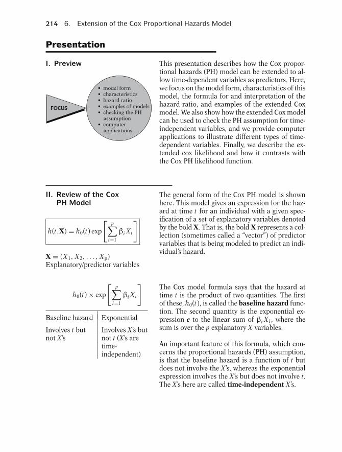
214 6. Extension of the Cox Proportional Hazards Model
Presentation
I. Preview This presentation describes how the Cox propor-tional hazards (PH) model can be extended to al-low time-dependent variables as predictors. Here,we focus on the model form, characteristics of thismodel, the formula for and interpretation of thehazard ratio, and examples of the extended Coxmodel. We also show how the extended Cox modelcan be used to check the PH assumption for time-independent variables, and we provide computerapplications to illustrate different types of time-dependent variables. Finally, we describe the ex-tended cox likelihood and how it contrasts withthe Cox PH likelihood function.
FOCUS
• model form• characteristics• hazard ratio• examples of models• checking the PH assumption• computer applications
II. Review of the CoxPH Model
The general form of the Cox PH model is shownhere. This model gives an expression for the haz-ard at time t for an individual with a given spec-ification of a set of explanatory variables denotedby the bold X. That is, the bold X represents a col-lection (sometimes called a “vector”) of predictorvariables that is being modeled to predict an indi-vidual’s hazard.
h(t,X) = h0(t) exp
[p∑
i=1
βi Xi
]
X = (X1, X2, . . . , Xp)Explanatory/predictor variables
h0(t) × exp
[p∑
i=1
βi Xi
]
Baseline hazard Exponential
Involves t but Involves X ’s butnot X ’s not t (X ’s are
time-independent)
The Cox model formula says that the hazard attime t is the product of two quantities. The firstof these, h0(t), is called the baseline hazard func-tion. The second quantity is the exponential ex-pression e to the linear sum of βi Xi , where thesum is over the p explanatory X variables.
An important feature of this formula, which con-cerns the proportional hazards (PH) assumption,is that the baseline hazard is a function of t butdoes not involve the X ’s, whereas the exponentialexpression involves the X ’s but does not involve t.The X ’s here are called time-independent X ’s.
Presentation: II. Review of the Cox PH Model 215
X ’s involving t: time dependent
Requires extended Cox model(no PH)
It is possible, nevertheless, to consider X ’s thatdo involve t. Such X ’s are called time-dependentvariables. If time-dependent variables are consid-ered, the Cox model form may still be used, butsuch a model no longer satisfies the PH assump-tion and is called the extended Cox model. Wewill discuss time-dependent variables and the cor-responding extended Cox model beginning in thenext section.
Hazard ratio formula:
HR = exp
[p∑
i=1
βi (X ∗i − Xi )
]where X∗ = (X ∗
1, X ∗2, . . . , X ∗
p) andX = (X1, X2, . . . , X p) denote thetwo sets of X ’s.
From the Cox PH model, we can obtain a gen-eral formula, shown here, for estimating a hazardratio that compares two specifications of the X ’s,defined as X∗ and X.
PH assumption:
h (t,X∗)
h (t,X)= θ (a constant over t)
i.e., h (t,X∗) = θh (t,X)
The (PH) assumption underlying the Cox PHmodel is that the hazard ratio comparing anytwo specifications of X predictors is constant overtime. Equivalently, this means that the hazard forone individual is proportional to the hazard forany other individual, where the proportionalityconstant is independent of time.
Hazards cross ⇒ PH not met
Hazards don’t cross ⇒\ PH met
An example of when the PH assumption is not metis given by any study situation in which the haz-ards for two or more groups cross when graphedagainst time. However, even if the hazard func-tions do not cross, it is possible that the PH as-sumption is not met.
Three approaches:
� graphical� time-dependent variables� goodness-of-fit test
As described in more detail in Chapter 4, thereare three general approaches for assessing the PHassumption. These are
� a graphical approach;� the use of time-dependent variables in an ex-tended Cox model; and� the use of a goodness-of-fit test.
Time-dependent covariates:
Extend Cox model: add productterm(s) involving some function oftime
When time-dependent variables are used to assessthe PH assumption for a time-independent vari-able, the Cox model is extended to contain prod-uct (i.e., interaction) terms involving the time-independent variable being assessed and somefunction of time.

216 6. Extension of the Cox Proportional Hazards Model
h(t,X) = h0(t) exp[β1sex + β2(sex × t)]
EXAMPLE
H0:β2 = 0 ⇒ PH assumption satisfied
For example, if the PH assumption is being as-sessed for gender, a Cox model might be extendedto include the variable sex × t in addition to sex.If the coefficient of the product term turns out tobe non-significant, we can conclude that the PHassumption is satisfied for sex provided that thevariable sex × t is an appropriate choice of time-dependent variable.
Options when PH assumption notsatisfied:
� Use a stratified Cox (SC) model.� Use time-dependent variables.
There are two options to consider if the PH as-sumption is not satisfied for one or more of thepredictors in the model. In Chapter 5, we de-scribed the option of using a stratified Cox (SC)model, which stratifies on the predictor(s) not sat-isfying the PH assumption, while keeping in themodel those predictors that satisfy the PH as-sumption. In this chapter, we describe the otheroption, which involves using time-dependent vari-ables.
Time-dependent variables may be:
� inherently time-dependent� defined to analyze a time-independent predictor notsatisfying the PH assumption.
Note that a given study may consider predictorsthat are inherently defined as time-dependent, aswe will illustrate in the next section. Thus, in addi-tion to considering time-dependent variables as anoption for analyzing a time-independent variablenot satisfying the PH assumption, we also discusspredictors which are inherently defined as time-dependent.
III. Definition and Examplesof Time-DependentVariables
A time-dependent variable is defined as any vari-able whose value for a given subject may differover time (t). In contrast, a time-independent vari-able is a variable whose value for a given subjectremains constant over time.
As a simple example, the variable RACE is atime-independent variable, whereas the variableRACE × time is a time-dependent variable.
Definition:
Time-dependent Time-independent
Value of variable Value of variablediffers over time is constant over
time
Example:��
��Race × t
��
�Race

Presentation: III. Definition and Examples of Time-Dependent Variables 217
EXAMPLES OFDEFINED VARIABLES
Defined variable: RACE × t
Time-independentRace = 1 ⇒ Race × t = tRace = 0 ⇒ Race × t = 0 (at any t)
E × (log t – 3){
{
Function of t
[E denotes a (0,1) exposure variable].
E × g(t) where g(t) = 1 if t ≥ t00 if t < t0
Heavyside function
t ≥ t0: E × g(t) = E
t < t0: E × g(t) = 0
1
0
Heavyside functions used when PHassumptions not met.
The variable RACE × time is an example of what iscalled a “defined” time-dependent variable. Mostdefined variables are of the form of the product of atime-independent variable (e.g., RACE) multipliedby time or some function of time. Note that afterRACE is determined for a given subject, all the val-ues of the RACE × time variable are completelydefined over a specified time interval of study.
A second example of a defined variable is given byE× (log t − 3), where E denotes, say, a (0,1) expo-sure status variable determined at one’s entry intothe study. Notice that here we have used a func-tion of time—that is, log t − 3—rather than timealone.
Yet another example of a defined variable, whichalso involves a function of time, is given by E ×g (t), where g (t) is defined to take on the value 1 ift is greater than or equal to some specified valueof t, called t0, and takes on the value 0 if t is lessthan t0.
The function g (t) is called a “heaviside” function.Note that whenever t is greater than or equal tot0, g (t) equals 1, so E × g (t) = E; however, when-ever t is less than t0, g (t) = 0, so the value ofE × g (t) is always 0. We will later return to illus-trate how heaviside functions may be used as onemethod for the analysis when a time-independentvariable like E does not satisfy the proportionalhazards assumption.
Internal variable: Another type of time-dependent variable is calledan “internal” variable. Examples of such a variableinclude exposure level E at time t, employmentstatus (EMP) at time t, smoking status (SMK) attime t, and obesity level (OBS) at time t.
EXAMPLES OF INTERNALVARIABLESE(t), EMP(t), SMK(t), OBS(t),
Values change because of “internal”characteristics or behavior of the in-dividual.
All these examples consider variables whose val-ues may change over time for any subject understudy; moreover, for internal variables, the reasonfor a change in value depends on “internal” char-acteristics or behavior specific to the individual.

218 6. Extension of the Cox Proportional Hazards Model
“Ancillary” variable:Value changes because of “external”characteristics.
In contrast, a variable is called an “ancillary” vari-able if its value changes primarily because of “ex-ternal” characteristics of the environment thatmay affect several individuals simultaneously. Anexample of an ancillary variable is air pollutionindex at time t for a particular geographical area.Another example is employment status (EMP) attime t, if the primary reason for whether some-one is employed or not depends more on generaleconomic circumstances than on individual char-acteristics.
EXAMPLES OF ANCILLARY VARIABLES
Air pollution index at time t; EMP(t)
ANOTHER EXAMPLEHeart transplant status at time t:
Transplant
Heart transplant status = HT(t)
Internal:Status determinedfrom individualtraits
Ancillary:Status determinedfrom externalavailability of adonor
HT(t) = 1 if received transplant at some time t0 ≤ t0 if did not receive transplant by time t
HT(t): 0000...0 111111111
t0t
T
T
HT(t):No transplant HT(t): 0000...00000
t
As another example, which may be part internaland part ancillary, we consider heart transplantstatus (HT) at time t for a person identified to havea serious heart condition, making him or her el-igible for a transplant. The value of this variableHT at time t is 1 if the person has already receiveda transplant at some time, say t0, prior to time t.The value of HT is 0 at time t if the person has notyet received a transplant by time t.
Note that once a person receives a transplant,at time t0, the value of HT remains at 1 for allsubsequent times. Thus, for a person receiving atransplant, the value of HT is 0 up to the time oftransplant, and then remains at 1 thereafter. Incontrast, a person who never receives a transplanthas HT equal to 0 for all times during the periodhe or she is in the study.
The variable “heart transplant status,” HT(t), canbe considered essentially an internal variable, be-cause individual traits of an eligible transplant re-cipient are important determinants of the decisionto carry out transplant surgery. Nevertheless, theavailability of a donor heart prior to tissue andother matching with an eligible recipient can beconsidered an “ancillary” characteristic externalto the recipient.
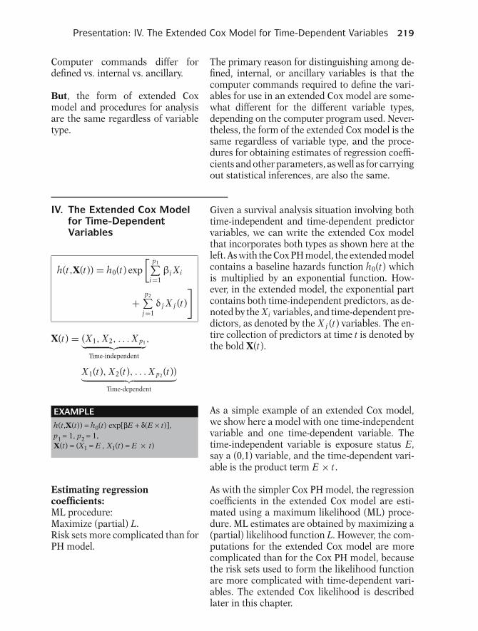
Presentation: IV. The Extended Cox Model for Time-Dependent Variables 219
Computer commands differ fordefined vs. internal vs. ancillary.
But, the form of extended Coxmodel and procedures for analysisare the same regardless of variabletype.
The primary reason for distinguishing among de-fined, internal, or ancillary variables is that thecomputer commands required to define the vari-ables for use in an extended Cox model are some-what different for the different variable types,depending on the computer program used. Never-theless, the form of the extended Cox model is thesame regardless of variable type, and the proce-dures for obtaining estimates of regression coeffi-cients and other parameters, as well as for carryingout statistical inferences, are also the same.
IV. The Extended Cox Modelfor Time-DependentVariables
Given a survival analysis situation involving bothtime-independent and time-dependent predictorvariables, we can write the extended Cox modelthat incorporates both types as shown here at theleft. As with the Cox PH model, the extended modelcontains a baseline hazards function h0(t) whichis multiplied by an exponential function. How-ever, in the extended model, the exponential partcontains both time-independent predictors, as de-noted by the Xi variables, and time-dependent pre-dictors, as denoted by the X j (t) variables. The en-tire collection of predictors at time t is denoted bythe bold X(t).
h(t,X(t)) = h0(t) exp[ p1∑
i=1βi Xi
+p2∑
j=1δ j X j (t)
]
X(t) = (X1, X2, . . . X p1︸ ︷︷ ︸Time-independent
,
X1(t), X2(t), . . . X p2 (t))︸ ︷︷ ︸Time-dependent
h(t,X(t)) = h0(t) exp[βE + δ(E × t)],
EXAMPLE
p1 = 1, p2 = 1,X(t) = (X1 = E , X1(t) = E × t)
As a simple example of an extended Cox model,we show here a model with one time-independentvariable and one time-dependent variable. Thetime-independent variable is exposure status E,say a (0,1) variable, and the time-dependent vari-able is the product term E × t.
Estimating regressioncoefficients:ML procedure:Maximize (partial) L.Risk sets more complicated than forPH model.
As with the simpler Cox PH model, the regressioncoefficients in the extended Cox model are esti-mated using a maximum likelihood (ML) proce-dure. ML estimates are obtained by maximizing a(partial) likelihood function L. However, the com-putations for the extended Cox model are morecomplicated than for the Cox PH model, becausethe risk sets used to form the likelihood functionare more complicated with time-dependent vari-ables. The extended Cox likelihood is describedlater in this chapter.
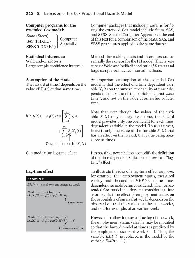
220 6. Extension of the Cox Proportional Hazards Model
Computer programs for theextended Cox model:
Stata (Stcox)SAS (PHREG)SPSS (COXREG)
⎫⎬⎭ ComputerAppendix
Computer packages that include programs for fit-ting the extended Cox model include Stata, SAS,and SPSS. See the Computer Appendix at the endof this text for a comparison of the Stata, SAS, andSPSS procedures applied to the same dataset.
Statistical inferences:Wald and/or LR testsLarge sample confidence intervals
Methods for making statistical inferences are es-sentially the same as for the PH model. That is, onecan use Wald and/or likelihood ratio (LR) tests andlarge sample confidence interval methods.
Assumption of the model:The hazard at time t depends on thevalue of X j (t) at that same time.
An important assumption of the extended Coxmodel is that the effect of a time-dependent vari-able X j (t) on the survival probability at time t de-pends on the value of this variable at that sametime t, and not on the value at an earlier or latertime.
h(t,X(t)) = h0(t) exp
[p1∑
i=1
βi Xi
+p2∑
j=1
δ j X j (t)
]↑
One coefficient forX j (t)
Note that even though the values of the vari-able X j (t) may change over time, the hazardmodel provides only one coefficient for each time-dependent variable in the model. Thus, at time t,there is only one value of the variable X j (t) thathas an effect on the hazard, that value being mea-sured at time t.
Can modify for lag-time effect It is possible, nevertheless, to modify the definitionof the time-dependent variable to allow for a “lag-time” effect.
Lag-time effect:
EMP(t) = employment status at week t
EXAMPLE
Model without lag-time:
Same week
h(t,X(t)) = h0(t) exp[δEMP(t)]
One-week earlier
Model with 1-week lag-time:h(t,X(t)) = h0(t) exp[δ∗EMP(t – 1)]
To illustrate the idea of a lag-time effect, suppose,for example, that employment status, measuredweekly and denoted as EMP (t), is the time-dependent variable being considered. Then, an ex-tended Cox model that does not consider lag-timeassumes that the effect of employment status onthe probability of survival at week t depends on theobserved value of this variable at the same week t,and not, for example, at an earlier week.
However, to allow for, say, a time-lag of one week,the employment status variable may be modifiedso that the hazard model at time t is predicted bythe employment status at week t − 1. Thus, thevariable EMP (t) is replaced in the model by thevariable EMP (t − 1).

Presentation: V. The Hazard Ratio Formula for the Extended Cox Model 221
General lag-time extended model:
h(t,X(t)) = h0(t) exp
[p1∑
i=1
βi Xi
+p2∑
j=1
δ j X j (t − L j )
]↗
X j (t − L j ) replaces X j (t)
More generally, the extended Cox model may bealternatively written to allow for a lag-time modi-fication of any time-dependent variable of interest.If we let L j denote the lag-time specified for time-dependent variable j, then the general “lag-timeextended model” can be written as shown here.Note that the variable X j (t) in the earlier versionof the extended model is now replaced by the vari-able X j (t − L j ).
V. The Hazard Ratio Formulafor the ExtendedCox Model
We now describe the formula for the hazard ra-tio that derives from the extended Cox model.The most important feature of this formula isthat the proportional hazards assumption is nolonger satisfied when using the extended Coxmodel.
The general hazard ratio formula for the extendedCox model is shown here. This formula describesthe ratio of hazards at a particular time t, and re-quires the specification of two sets of predictorsat time t. These two sets are denoted as bold X∗(t)and bold X(t).
The two sets of predictors, X∗(t) and X(t), identifytwo specifications at time t for the combined set ofpredictors containing both time-independent andtime-dependent variables. The individual compo-nents for each set of predictors are shown here.
PH assumption is not satisfied forthe extended Cox model.
HR(t) = h (t,X∗(t))
h (t,X(t))
= exp
[p1∑
i=1
βi
[X ∗
i − Xi]
+p2∑
j=1
δ j[X ∗
j (t) − X j (t)]]
Two sets of predictors:
X∗(t) = (X ∗1, X ∗
2, . . . , X ∗p1
, X ∗1(t),
X ∗2(t), . . . , X ∗
p2(t))
X(t) = (X1, X2, . . . , X p1, X1(t),X2(t), . . . , X p2 (t))

222 6. Extension of the Cox Proportional Hazards Model
h(t,X(t)) = h0(t) exp[βE + δ(E × t)]
EXAMPLE
E = { 1 if exposed 0 if unexposed
X*(t) = (E = 1, E × t = t)X(t) = (E = 0, E × t = 0)
HR(t) =ˆ h(t, E = 1)
h(t, E = 0)= exp[β(1 – 0) + δ((1 × t) – (0 × t))]= exp[β + δt]
δ > 0 ⇒ HR(t) ↑ as t ↑PH assumption not satisfied
ˆ
As a simple example, suppose the model containsonly one time-independent predictor, namely, ex-posure status E, a (0,1) variable, and one time-dependent predictor, namely, E × t. Then, to com-pare exposed persons, for whom E = 1, withunexposed persons, for whom E = 0, at timet, the bold X∗(t) set of predictors has as itstwo components E = 1 and E × t = t; the boldX(t) set has as its two components E = 0 andE × t = 0.
If we now calculate the estimated hazard ratio thatcompares exposed to unexposed persons at timet, we obtain the formula shown here; that is, HR“hat” equals the exponential of β “hat” plus δ “hat”times t. This formula says that the hazard ratio isa function of time; in particular, if δ “hat” is posi-tive, then the hazard ratio increases with increas-ing time. Thus, the hazard ratio in this example iscertainly not constant, so that the PH assumptionis not satisfied for this model.
HR(t) = exp
[p1∑
i=1
βi
[X ∗
i − Xi]
+p2∑
j=1
δ j
��
��
[X ∗
j (t) − X j (t)] ]
↗A function of time
More generally, because the general hazard ratioformula involves differences in the values of thetime-dependent variables at time t, this hazard ra-tio is a function of time. Thus, in general, the ex-tended Cox model does not satisfy the PH assump-tion if any δ j is not equal to zero.
In general, PH assumption not sat-isfied for extended Cox model.
δ j is not time-dependent.
δ j represents “overall” effect ofX j (t).
Note that, in the hazard ratio formula, the co-efficient δ j “hat” of the difference in valuesof the jth time-dependent variable is itself nottime-dependent. Thus, this coefficient representsthe “overall” effect of the corresponding time-dependent variable, considering all times at whichthis variable has been measured in the study.

Presentation: V. The Hazard Ratio Formula for the Extended Cox Model 223
EXAMPLEE(t) = chemical exposure status at time t (weekly)
= 0 if unexposed at time t1 if exposed at time t
A
B
:
:
E(t) 0 1 0 1 1
t 1 2 3 4 5...
E(t) 1 1 0 1 0
t 1 2 3 4 5...
Exposed vs. unexposedE = 1 E = 0
h(t,X(t)) = h0(t) exp[δE(t)]
One coefficient
δ represents the overall effect of E(t).
......
{
= eδ, a fixed number
HR(t) = ˆh(t,E(t) = 0)
h(t,E(t) = 1)
= exp[δ[1 – 0]]
ˆBut, PH is not satisfied:HR(t) is time-dependent because E(t) istime-dependent.
As another example to illustrate the formula forthe hazard ratio, consider an extended Cox modelcontaining only one variable, say a weekly mea-sure of chemical exposure status at time t. Sup-pose this variable, denoted as E(t), can take one oftwo values, 0 or 1, depending on whether a personis unexposed or exposed, respectively, at a givenweekly measurement.
As defined, the variable E(t) can take on differ-ent patterns of values for different subjects. Forexample, for a five-week period, subject A’s valuesmay be 01011, whereas subject B’s values may be11010.
Note that in this example, we do not considertwo separate groups of subjects, with one groupalways exposed and the other group always un-exposed throughout the study. This latter situa-tion would require a (0,1) time-independent vari-able for exposure, whereas our example involvesa time-dependent exposure variable.
The extended Cox model that includes only thevariable E(t) is shown here. In this model, the val-ues of the exposure variable may change over timefor different subjects, but there is only one coeffi-cient, δ, corresponding to the one variable in themodel. Thus, δ represents the overall effect on sur-vival time of the time-dependent variable E(t).
Notice, also, that the hazard ratio formula, whichcompares an exposed person to an unexposed per-son at time t, yields the expression e to the δ “hat.”
Although this result is a fixed number, the PH as-sumption is not satisfied. The fixed number givesthe hazard ratio at a given time, assuming that theexposure status at that time is 1 in the numeratorand is 0 denominator. Thus, the hazard ratio istime-dependent, because exposure status is time-dependent, even though the formula yields a singlefixed number.

224 6. Extension of the Cox Proportional Hazards Model
VI. Assessing Time-Independent VariablesThat Do Not Satisfy thePH Assumption
Use an extended Cox model to
� check PH assumption;� assess effect of variable notsatisfying PH assumption.
We now discuss how to use an extended Cox modelto check the PH assumption for time-independentvariables and to assess the effect of a variable thatdoes not satisfy the PH assumption.
Three methods for checking PH as-sumption:
1. graphical2.
��
��extended Cox model
3. GOF test
As described previously (see Chapter 4), there arethree methods commonly used to assess the PHassumption: (1) graphical, using, say, log–log sur-vival curves; (2) using an extended Cox model; and(3) using a goodness-of-fit (GOF) test. We have pre-viously (in Chapter 4) discussed items 1 and 3, butonly briefly described item 2, which we focus onhere.
Cox PH model for p time-independent X ’s:
h(t,X) = h0(t) exp
[p∑
i=1
βi Xi
]If the dataset for our study contains several, say p,time-independent variables, we might wish to fit aCox PH model containing each of these variables,as shown here.
Extended Cox model:Add product terms of the form:
Xi × gi (t)
However, to assess whether such a PH model isappropriate, we can extend this model by defin-ing several product terms involving each time-independent variable with some function of time.That is, if the ith time-independent variable is de-noted as Xi , then we can define the ith productterm as Xi × gi (t) where gi (t) is some function oftime for the ith variable.
h(t,X(t)) = h0(t) exp[ p∑
i=1βi Xi
+p∑
i=1δi Xi gi (t)
]The extended Cox model that simultaneously con-siders all time-independent variables of interest isshown here.

Presentation: VI. Assessing Time-Independent Variables 225
EXAMPLE
gi(t) = 0 for all i implies no time- dependent variable involving Xi, i.e.,
h(t,X(t)) = h0(t) expp
i=1ΣβiXi[ ]
In using this extended model, the crucial decisionis the form that the functions gi (t) should take.The simplest form for gi (t) is that all gi (t) areidentically 0 at any time; this is another way ofstating the original PH model, containing no time-dependent terms.
EXAMPLE 2
gi(t) = t ⇒ Xigi(t) = Xi × t
h(t,X(t)) = h0(t) expp
i=1ΣβiXi + Σδi(Xi × t)[ ] p
i=1
Another choice for the gi (t) is to let gi (t) = t. Thisimplies that for each Xi in the model as a main ef-fect, there is a corresponding time-dependent vari-able in the model of the form Xi × t. The extendedCox model in this case takes the form shown here.
EXAMPLE 3: one variable at a time
XL only ⇒ { gL(t) = t,
gi(t) = 0 for other i
h(t,X(t)) = h0(t) exp[ βiXi + δL(XL × t)]∑p
i=1
Suppose, however, we wish to focus on a partic-ular time-independent variable, say, variable X L .Then gi (t) = t for i = L , but equals 0 for all otheri. The corresponding extended Cox model wouldthen contain only one product term X L × t, asshown here.
h(t,X(t)) = h0(t) exp[ βiXi + δ i(Xi × ln t)]gi(t) = ln t ⇒ Xigi(t) = Xi × ln t
∑ ∑p p
i=1 i=1
EXAMPLE 4 Another choice for the gi (t) is the log of t, ratherthan simply t, so that the corresponding time-dependent variables will be of the form Xi × ln t.
EXAMPLE 5: Heaviside Function
gi(t) =0 if t ≥ t01 if t < t0
{And yet another choice would be to let gi (t) be a“heaviside function” of the form gi (t) = 1 whent is at or above some specified time, say t0, andgi (t) = 0 when t is below t0. We will discuss thischoice in more detail shortly.
Extended Cox model:
h(t,X(t)) = h0(t) exp
[p∑
i=1
βi Xi
+p∑
i=1
δi Xi gi (t)
]� Check PH assumption.� Obtain hazard ratio when PH
assumption not satisfied.
H0 : δ1 = δ2 = · · · = δp = 0
Given a particular choice of the gi (t), the corre-sponding extended Cox model, shown here againin general form, may then be used to check the PHassumption for the time-independent variables inthe model. Also, we can use this extended Coxmodel to obtain a hazard ratio formula that con-siders the effects of variables not satisfying the PHassumption.
To check the PH assumption using a statisticaltest, we consider the null hypothesis that all the δterms, which are coefficients of the Xi gi (t) prod-uct terms in the model, are zero.
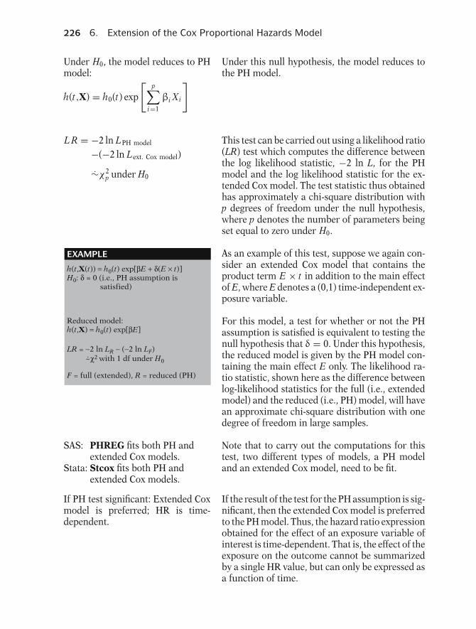
226 6. Extension of the Cox Proportional Hazards Model
Under H0, the model reduces to PHmodel:
h(t,X) = h0(t) exp
[p∑
i=1
βi Xi
] Under this null hypothesis, the model reduces tothe PH model.
L R = −2 ln LPH model
−(−2 ln Lext. Cox model)
∼χ2p under H0
This test can be carried out using a likelihood ratio(LR) test which computes the difference betweenthe log likelihood statistic, −2 ln L, for the PHmodel and the log likelihood statistic for the ex-tended Cox model. The test statistic thus obtainedhas approximately a chi-square distribution withp degrees of freedom under the null hypothesis,where p denotes the number of parameters beingset equal to zero under H0.
EXAMPLE
h(t,X(t)) = h0(t) exp[βE + δ(E × t)]H0: δ = 0 (i.e., PH assumption is
satisfied)
Reduced model:h(t,X) = h0(t) exp[βE]
LR = −2 ln LR − (−2 ln LF)~χ2 with 1 df under H0.
F = full (extended), R = reduced (PH)
As an example of this test, suppose we again con-sider an extended Cox model that contains theproduct term E × t in addition to the main effectof E, where E denotes a (0,1) time-independent ex-posure variable.
For this model, a test for whether or not the PHassumption is satisfied is equivalent to testing thenull hypothesis that δ = 0. Under this hypothesis,the reduced model is given by the PH model con-taining the main effect E only. The likelihood ra-tio statistic, shown here as the difference betweenlog-likelihood statistics for the full (i.e., extendedmodel) and the reduced (i.e., PH) model, will havean approximate chi-square distribution with onedegree of freedom in large samples.
SAS: PHREG fits both PH andextended Cox models.
Stata: Stcox fits both PH andextended Cox models.
Note that to carry out the computations for thistest, two different types of models, a PH modeland an extended Cox model, need to be fit.
If PH test significant: Extended Coxmodel is preferred; HR is time-dependent.
If the result of the test for the PH assumption is sig-nificant, then the extended Cox model is preferredto the PH model. Thus, the hazard ratio expressionobtained for the effect of an exposure variable ofinterest is time-dependent. That is, the effect of theexposure on the outcome cannot be summarizedby a single HR value, but can only be expressed asa function of time.
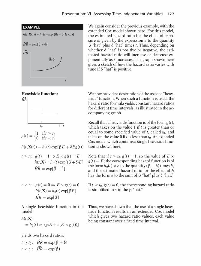
Presentation: VI. Assessing Time-Independent Variables 227
EXAMPLE
h(t,X(t)) = h0(t) exp[βE + δ(E × t)]
t
HR = exp[β + δt]
HR
δ>0
We again consider the previous example, with theextended Cox model shown here. For this model,the estimated hazard ratio for the effect of expo-sure is given by the expression e to the quantityβ “hat” plus δ “hat” times t. Thus, depending onwhether δ “hat” is positive or negative, the esti-mated hazard ratio will increase or decrease ex-ponentially as t increases. The graph shown heregives a sketch of how the hazard ratio varies withtime if δ “hat” is positive.
Heaviside function:
t0 t
HR
g (t) ={
1 if t ≥ t00 if t < t0
h(t,X(t)) = h0(t) exp[βE + δEg (t)]
We now provide a description of the use of a “heav-iside” function. When such a function is used, thehazard ratio formula yields constant hazard ratiosfor different time intervals, as illustrated in the ac-companying graph.
Recall that a heaviside function is of the form g (t),which takes on the value 1 if t is greater than orequal to some specified value of t, called t0, andtakes on the value 0 if t is less than t0. An extendedCox model which contains a single heaviside func-tion is shown here.
t ≥ t0: g (t) = 1 ⇒ E × g (t) = Eh(t,X) = h0(t) exp[(β+δ)E]
HR = exp[β + δ]
Note that if t ≥ t0, g (t) = 1, so the value of E ×g (t) = E; the corresponding hazard function is ofthe form h0(t) × e to the quantity (β + δ) times E,and the estimated hazard ratio for the effect of Ehas the form e to the sum of β “hat” plus δ “hat.”
t < t0: g (t) = 0 ⇒ E × g (t) = 0h(t,X) = h0(t) exp[βE]
HR = exp[β]
If t < t0, g (t) = 0, the corresponding hazard ratiois simplified to e to the β “hat.”
A single heaviside function in themodel
h(t,X)= h0(t) exp[βE + δ(E × g (t))]
yields two hazard ratios:
t ≥ t0 : HR = exp(β + δ)
t < t0 : HR = exp(β)
Thus, we have shown that the use of a single heav-iside function results in an extended Cox modelwhich gives two hazard ratio values, each valuebeing constant over a fixed time interval.

228 6. Extension of the Cox Proportional Hazards Model
Alternative model with two heavi-side functions:
h(t,X) = h0(t) exp[δ1(E × g1(t))+ δ2(E × g2(t))]
g1(t) ={
1 if t ≥ t00 if t < t0
g2(t) ={
1 if t < t00 if t ≥ t0
Note: Main effect for E not in model.
There is actually an equivalent way to write thismodel that uses two heaviside functions in thesame model. This alternative model is shown here.The two heaviside functions are called g1(t) andg2(t). Each of these functions are in the model aspart of a product term with the exposure variableE. Note that this model does not contain a maineffect term for exposure.
Two HR’s from the alternativemodel:
t ≥ t0 : g1(t) = 1, g2(t) = 0h(t,X) = h0(t) exp[δ1(E × 1)
+ δ2(E × 0)]= h0(t) exp[δ1 E]
so that HR = exp(δ1)
For this alternative model, as for the earlier modelwith only one heaviside function, two differenthazard ratios are obtained for different time inter-vals. To obtain the first hazard ratio, we considerthe form that the model takes when t ≥ t0. In thiscase, the value of g1(t) is 1 and the value of g2(t)is 0, so the exponential part of the model simpli-fies to δ1 × E; the corresponding formula for theestimated hazard ratio is then e to the δ1 “hat.”
t < t0 : g1(t) = 0, g2(t) = 1h(t,X) = h0(t) exp[δ1(E × 0)
+ δ2(E × 1)]= h0(t) exp[δ2 E]
so that HR = exp(δ2)
When t < t0, the value of g1(t) is 0 and the value ofg2(t) is 1. Then, the exponential part of the modelbecomes δ2 × E, and the corresponding hazardratio formula is e to the δ2 “hat.”
Alternative model:
h(t,X(t)) = h0(t) exp[δ1(E × g1(t))+ δ2(E × g2(t))]
Original model:
h(t,X(t))= h0(t) exp[βE + δ(E × g (t))]
t ≥ t0 : HR = exp(δ1) = exp(β + δ)
t < t0 : HR = exp(δ2) = exp(β)
Thus, using the alternative model, again shownhere, we obtain two distinct hazard ratio values.Mathematically, these are the same values as ob-tained from the original model containing onlyone heaviside function. In other words, δ1 “hat” inthe alternative model equals β “hat” plus δ “hat” inthe original model (containing one heaviside func-tion), and δ2 “hat” in the alternative model equalsβ “hat” in the original model.

Presentation: VI. Assessing Time-Independent Variables 229
Heaviside functions:
� two HR’s constant within twotime intervals� extension: several HR’s constantwithin several time intervals
We have thus seen that heaviside functions canbe used to provide estimated hazard ratios thatremain constant within each of two separate timeintervals of follow-up. We can also extend the useof heaviside functions to provide several distincthazard ratios that remain constant within severaltime intervals.
Four time intervals:
HR
0 .5 1.0 1.5 t (years)
Extended Cox model contains either
� E, E × g1(t), E × g2(t),E × g3(t)or� E × g1(t), E × g2(t), E ×g3(t), E × g4(t)
| 1 | 2 | 3 | 4−−−−−−−−−−−−−−−0 0.5 1.0 1.5 t(years)
Suppose, for instance, that we wish to separate thedata into four separate time intervals, and for eachinterval we wish to obtain a different hazard ratioestimate as illustrated in the graph shown here.
We can obtain four different hazard ratios usingan extended Cox model containing a main effect ofexposure and three heaviside functions in the modelas products with exposure. Or, we can use a modelcontaining no main effect exposure term, but withproduct terms involving exposure with four heav-iside functions.
To illustrate the latter model, suppose, as shownon the graph, that the first time interval goes fromtime 0 to 0.5 of a year; the second time intervalgoes from 0.5 to 1 year; the third time interval goesfrom 1 year to a year and a half; and the fourthtime interval goes from a year and a half onward.
h(t,X(t))= h0(t) exp[δ1 Eg1(t) + δ2 Eg2(t)
+δ3 Eg3(t) + δ4 Eg4(t)]
where
g1(t) ={
1 if 0 ≤ t < 0.5 year0 if otherwise
g2(t) ={
1 if 0.5 year ≤ t < 1.0 year0 if otherwise
g3(t) ={
1 if 1.0 year ≤ t < 1.5 years0 if otherwise
g4(t) ={
1 if t ≥ 1.5 years0 if otherwise
Then, an appropriate extended Cox model con-taining the four heaviside functions g1(t), g2(t),g3(t), and g4(t) is shown here. This model assumesthat there are four different hazard ratios identi-fied by three cutpoints at half a year, one year, andone and a half years. The formulae for the fourhazard ratios are given by separately exponenti-ating each of the four estimated coefficients, asshown below:
4 HR’s
⎧⎪⎪⎨⎪⎪⎩0 ≤ t < 0.5: HR = exp(δ1)0.5 ≤ t < 1.0: HR = exp(δ2)1.0 ≤ t < 1.5: HR = exp(δ3)t ≥ 1.5: HR = exp(δ4)

230 6. Extension of the Cox Proportional Hazards Model
VII. An Application of theExtended Cox Model toAn Epidemiologic Studyon the Treatment ofHeroin Addiction
A 1991 Australian study by Caplehorn et al., com-pared retention in two methadone treatment clin-ics for heroin addicts. A patient’s survival time(T) was determined as the time in days until thepatient dropped out of the clinic or was cen-sored at the end of the study clinic. The two clin-ics differed according to their overall treatmentpolicies.
A listing of some of the variables in the datasetfor this study is shown here. The dataset name iscalled “ADDICTS,” and survival analysis programsin the Stata package are used in the analysis. Notethat the survival time variable is listed in column4 and the survival status variable, which indicateswhether a patient departed from the clinic or wascensored, is listed in column 3. The primary ex-posure variable of interest is the clinic variable,which is coded as 1 or 2. Two other variables of in-terest are prison record status, listed in column 5and coded as 0 if none and 1 if any, and maximummethadone dose, in milligrams per day, which islisted in column 6. These latter two variables areconsidered as covariates.
One of the first models considered in the analysisof the addicts dataset was a Cox PH model con-taining the three variables, clinic, prison record,and dose. An edited printout of the results for thismodel is shown here. What stands out from thisprintout is that the P(PH) value for the clinic vari-able is zero to three significant places, which in-dicates that the clinic variable does not satisfy theproportional hazard assumption.
Since the P(PH) values for the other two variablesin the model are highly nonsignificant, this sug-gests that these two variables, namely, prison anddose, can remain in the model.
EXAMPLE
Dataset name: ADDICTSColumn 1: Subject IDColumn 2: Clinic (1 or 2)Column 3: Survival status (0 = cen-
sored, 1 = departed clinic)Column 4: Survival time in daysColumn 5: Prison Record
(0 = none, 1 = any)Column 6: Maximum Methadone Dose
(mg/day)
E
covariates
h(t,X) = h0(t) exp[β1(clinic)+ β2(prison) + β3(dose)]
Coef. Std. Err. p> |z| Haz. Ratio P(PH)
ClinicPrisonDose
−1.009 0.327−0.035
0.2150.1670.006
0.0000.0510.000
0.3651.3860.965
0.0010.3320.347
P(PH) for the variables prison and dose arenonsignificant ⇒ remain in model
1991 Australian study (Caplehornet al.) of heroin addicts
• two methadone treatment clinics
• T = days remaining in treatment(= days until drop out of clinic)
• clinics differ in treatment policies

Presentation: VII. An Epidemiologic Study on the Treatment of Heroin Addiction 231
EXAMPLE (continued)
Results:
Stratifying by clinic: cannot obtain hazardratio for clinic
Hazard ratio for clinic requires clinic in themodel.
Adjusted Survival CurvesStratified by Clinic
(prison and dose in the model)
Clinic 2
Clinic 1
1
.8
.6
.4
.2
00 200 400 600 800 1000 1200
Days
S
h(t,X(t)) = h0(t) exp[β1(clinic)+ β2(prison) + β3(dose)+ δ(clinic)g(t)]
Extended Cox model:
t ≥ 365 days: HR = exp(β1 + δ)
t < 365 days: HR = exp(β1)
where
g(t) = 1 if t ≥ 365 days0 if t < 365 days{
clinic = { 1 if clinic 10 if clinic 2
and
Note:Previously
clinic = 2 forclinic 2
• Curve for clinic 2 consistently lies above curve for clinic 1.
• Curves diverge, with clinic 2 being vastly superior after one year.
Further evidence of the PH assumption not be-ing satisfied for the clinic variable can be seenfrom a graph of adjusted survival curves strati-fied by clinic, where the prison and dose variableshave been kept in the model. Notice that the twocurves are much closer together at earlier times,roughly less than one year (i.e., 365 days), but thetwo curves diverge greatly after one year. This in-dicates that the hazard ratio for the clinic variablewill be much closer to one at early times but quitedifferent from one later on.
The above graph, nevertheless, provides impor-tant results regarding the comparison of the twoclinics. The curve for clinic 2 consistently liesabove the curve for clinic 1, indicating that clinic2 does better than clinic 1 in retaining its patientsin methadone treatment. Further, because the twocurves diverge after about a year, it appears thatclinic 2 is vastly superior to clinic 1 after one yearbut only slightly better than clinic 1 prior to oneyear.
Unfortunately, because the clinic variable has beenstratified in the analysis, we cannot use this anal-ysis to obtain a hazard ratio expression for theeffect of clinic, adjusted for the effects of prisonand dose. We can only obtain such an expressionfor the hazard ratio if the clinic variable is in themodel.
Nevertheless, we can obtain a hazard ratio us-ing an alternative analysis with an extended Coxmodel that contains a heaviside function, g (t), to-gether with the clinic variable, as shown here.Based on the graphical results shown earlier, a log-ical choice for the cutpoint of the heaviside func-tion is one year (i.e., 365 days). The correspondingmodel then provides two hazard ratios: one that isconstant above 365 days and the other that is con-stant below 365 days.
Note that in the extended Cox model here, we havecoded the clinic variable as 1 if clinic 1 and 0 ifclinic 2, whereas previously we had coded clinic2 as 2. The reason for this change in coding, asillustrated by computer output below, is to obtainhazard ratio estimates that are greater than unity.
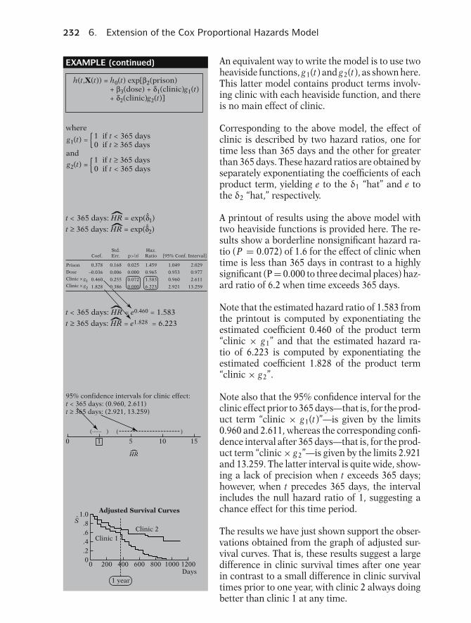
232 6. Extension of the Cox Proportional Hazards Model
EXAMPLE (continued)
h(t,X(t)) = h0(t) exp[β2(prison)+ β3(dose) + δ1(clinic)g1(t)+ δ2(clinic)g2(t)]
t < 365 days: HR = exp(δ1)
t ≥ 365 days: HR = exp(δ2)
where
g1(t) = { 1 if t < 365 days0 if t ≥ 365 days
g2(t) = { 1 if t ≥ 365 days0 if t < 365 days
and
ˆˆ
t < 365 days: HR = e0.460 = 1.583
t ≥ 365 days: HR = e1.828 = 6.223ˆˆ
Coef.
0.378
–0.036
0.460
1.828
Std.Err.
0.168
0.006
0.255
0.386
p>|z|
0.025
0.000
0.072
0.000
Haz.Ratio
1.459
0.965
1.583
6.223
[95% Conf. Interval]
1.049
0.953
0.960
2.921
2.029
0.977
2.611
13.259
Prison
Dose
Clinic × g1Clinic × g2
95% confidence intervals for clinic effect:t < 365 days: (0.960, 2.611)t ≥ 365 days: (2.921, 13.259)
(...... ) ( )
0 1 5 10 15
1 year
HR
1.0.8.6.4.20
0 200 400 600 800 1000 1200Days
Adjusted Survival Curves
Clinic 2Clinic 1
S
An equivalent way to write the model is to use twoheaviside functions, g1(t) and g2(t), as shown here.This latter model contains product terms involv-ing clinic with each heaviside function, and thereis no main effect of clinic.
Corresponding to the above model, the effect ofclinic is described by two hazard ratios, one fortime less than 365 days and the other for greaterthan 365 days. These hazard ratios are obtained byseparately exponentiating the coefficients of eachproduct term, yielding e to the δ1 “hat” and e tothe δ2 “hat,” respectively.
A printout of results using the above model withtwo heaviside functions is provided here. The re-sults show a borderline nonsignificant hazard ra-tio (P = 0.072) of 1.6 for the effect of clinic whentime is less than 365 days in contrast to a highlysignificant (P = 0.000 to three decimal places) haz-ard ratio of 6.2 when time exceeds 365 days.
Note that the estimated hazard ratio of 1.583 fromthe printout is computed by exponentiating theestimated coefficient 0.460 of the product term“clinic × g1” and that the estimated hazard ra-tio of 6.223 is computed by exponentiating theestimated coefficient 1.828 of the product term“clinic × g2”.
Note also that the 95% confidence interval for theclinic effect prior to 365 days—that is, for the prod-uct term “clinic × g1(t)”—is given by the limits0.960 and 2.611, whereas the corresponding confi-dence interval after 365 days—that is, for the prod-uct term “clinic × g2”—is given by the limits 2.921and 13.259. The latter interval is quite wide, show-ing a lack of precision when t exceeds 365 days;however, when t precedes 365 days, the intervalincludes the null hazard ratio of 1, suggesting achance effect for this time period.
The results we have just shown support the obser-vations obtained from the graph of adjusted sur-vival curves. That is, these results suggest a largedifference in clinic survival times after one yearin contrast to a small difference in clinic survivaltimes prior to one year, with clinic 2 always doingbetter than clinic 1 at any time.
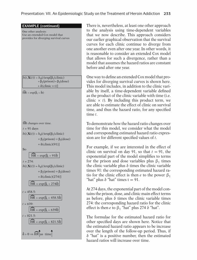
Presentation: VII. An Epidemiologic Study on the Treatment of Heroin Addiction 233
EXAMPLE (continued)One other analysis:Use an extended Cox model thatprovides for diverging survival curves
h(t,X(t)) = h0(t)exp[β1(clinic) +β2(prison)+β3(dose)
+ δ(clinic × t)]
HR = exp(β1 + δt)
So
t = 91 days
HR = exp(β1 + 91δ)ˆt = 274:
HR = exp(β1 + 274δ)ˆ
h(t,X(t)) = h0(t)exp[β1(clinic)
+ β2(prison) + β3(dose)
+ δ(clinic)(91)]
h(t,X(t)) = h0(t)exp[β1(clinic)
+ β2(prison) + β3(dose)
+ δ(clinic)(274)]
t = 458.5:
HR = exp(β1 + 458.5δ)ˆt = 639:
HR = exp(β1 + 639δ)ˆt = 821.5:
HR = exp(β1 + 821.5δ)ˆ
δ > 0 ⇒ HR as time ˆ
HR changes over time.
There is, nevertheless, at least one other approachto the analysis using time-dependent variablesthat we now describe. This approach considersour earlier graphical observation that the survivalcurves for each clinic continue to diverge fromone another even after one year. In other words, itis reasonable to consider an extended Cox modelthat allows for such a divergence, rather than amodel that assumes the hazard ratios are constantbefore and after one year.
One way to define an extended Cox model that pro-vides for diverging survival curves is shown here.This model includes, in addition to the clinic vari-able by itself, a time-dependent variable definedas the product of the clinic variable with time (i.e.clinic × t). By including this product term, weare able to estimate the effect of clinic on survivaltime, and thus the hazard ratio, for any specifiedtime t.
To demonstrate how the hazard ratio changes overtime for this model, we consider what the modeland corresponding estimated hazard ratio expres-sion are for different specified values of t.
For example, if we are interested in the effect ofclinic on survival on day 91, so that t = 91, theexponential part of the model simplifies to termsfor the prison and dose variables plus β1 timesthe clinic variable plus δ times the clinic variabletimes 91: the corresponding estimated hazard ra-tio for the clinic effect is then e to the power β1“hat” plus δ “hat” times t = 91.
At 274 days, the exponential part of the model con-tains the prison, dose, and clinic main effect termsas before, plus δ times the clinic variable times274: the corresponding hazard ratio for the cliniceffect is then e to β1 “hat” plus 274 δ “hat”.
The formulae for the estimated hazard ratio forother specified days are shown here. Notice thatthe estimated hazard ratio appears to be increaseover the length of the follow-up period. Thus, ifδ “hat” is a positive number, then the estimatedhazard ratios will increase over time.
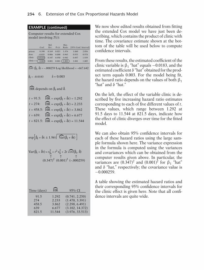
234 6. Extension of the Cox Proportional Hazards Model
EXAMPLE (continued)
Coef.
0.390
–0.035
–0.0183
0.003
Std.Err.
0.169
0.006
0.347
0.001
P>|z|
0.021
0.000
0.958
0.001
Haz.Ratio
1.476
0.965
0.982
1.003
[95% Conf. Interval]
1.060
0.953
0.497
1.001
2.056
0.978
1.939
1.005
prison
dose
clinic
clinic × t
HR depends on β1 and δ.ˆ
Computer results for extended Coxmodel involving T(t):
cov (β1, δ) = –.000259 Log likelihood = –667.642 ˆβ1 = –0.0183 δ = 0.003
t = 91.5: HR = exp(β1 + δt) = 1.292ˆt = 274: HR = exp(β1 + δt) = 2.233ˆt = 458.5: HR = exp(β1 + δt) = 3.862ˆt = 639: HR = exp(β1 + δt) = 6.677ˆt = 821.5: HR = exp(β1 + δt) = 11.544ˆ
exp β1 + δt ± 1.96 Var(β1 + δt)
Var(β1 + δt) = sβ1+ t2 sδ + 2t cov(β1, δ)
↑ ↑ ↑(0.347)2 (0.001)2 (–.000259)
ˆ
ˆ
Time (days)
91.5274458.5639 821.5
HR
1.2922.2333.8626.677
11.544
95% CI
(0.741, 2.250)(1.470, 3.391)(2.298, 6.491)
2 2
(3.102, 14.372)(3.976, 33.513)
We now show edited results obtained from fittingthe extended Cox model we have just been de-scribing, which contains the product of clinic withtime. The covariance estimate shown at the bot-tom of the table will be used below to computeconfidence intervals.
From these results, the estimated coefficient of theclinic variable is β1 “hat” equals −0.0183, and theestimated coefficient δ “hat” obtained for the prod-uct term equals 0.003. For the model being fit,the hazard ratio depends on the values of both β1“hat” and δ “hat.”
On the left, the effect of the variable clinic is de-scribed by five increasing hazard ratio estimatescorresponding to each of five different values of t.These values, which range between 1.292 at91.5 days to 11.544 at 821.5 days, indicate howthe effect of clinic diverges over time for the fittedmodel.
We can also obtain 95% confidence intervals foreach of these hazard ratios using the large sam-ple formula shown here. The variance expressionin the formula is computed using the variancesand covariances which can be obtained from thecomputer results given above. In particular, thevariances are (0.347)2 and (0.001)2 for β1 “hat”and δ “hat,” respectively; the covariance value is−0.000259.
A table showing the estimated hazard ratios andtheir corresponding 95% confidence intervals forthe clinic effect is given here. Note that all confi-dence intervals are quite wide.
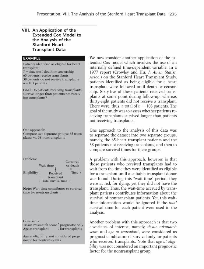
Presentation: VIII. The Analysis of the Stanford Heart Transplant Data 235
VIII. An Application of theExtended Cox Model tothe Analysis of theStanford HeartTransplant Data
EXAMPLEPatients identified as eligible for hearttransplant:T = time until death or censorship65 patients receive transplants38 patients do not receive transplantsn = 103 patients
Goal: Do patients receiving transplantssurvive longer than patients not receiv-ing transplants?
One approach:Compare two separate groups: 65 trans-plants vs. 38 nontransplants
Problem:
Wait-time
Eligibility
Censoredor death
↑Received
transplant← Total survival time →
×Time→
Note: Wait-time contributes to survivaltime for nontransplants.
Covariates:Tissue mismatch score prognostic onlyAge at transplant for transplants
Age at eligibility: not considered prog-nostic for nontransplants
}
We now consider another application of the ex-tended Cox model which involves the use of aninternally defined time-dependent variable. In a1977 report (Crowley and Hu, J. Amer. Statist.Assoc.) on the Stanford Heart Transplant Study,patients identified as being eligible for a hearttransplant were followed until death or censor-ship. Sixty-five of these patients received trans-plants at some point during follow-up, whereasthirty-eight patients did not receive a transplant.There were, thus, a total of n = 103 patients. Thegoal of the study was to assess whether patients re-ceiving transplants survived longer than patientsnot receiving transplants.
One approach to the analysis of this data wasto separate the dataset into two separate groups,namely, the 65 heart transplant patients and the38 patients not receiving transplants, and then tocompare survival times for these groups.
A problem with this approach, however, is thatthose patients who received transplants had towait from the time they were identified as eligiblefor a transplant until a suitable transplant donorwas found. During this “wait-time” period, theywere at risk for dying, yet they did not have thetransplant. Thus, the wait-time accrued by trans-plant patients contributes information about thesurvival of nontransplant patients. Yet, this wait-time information would be ignored if the totalsurvival time for each patient were used in theanalysis.
Another problem with this approach is that twocovariates of interest, namely, tissue mismatchscore and age at transplant, were considered asprognostic indicators of survival only for patientswho received transplants. Note that age at eligi-bility was not considered an important prognosticfactor for the nontransplant group.
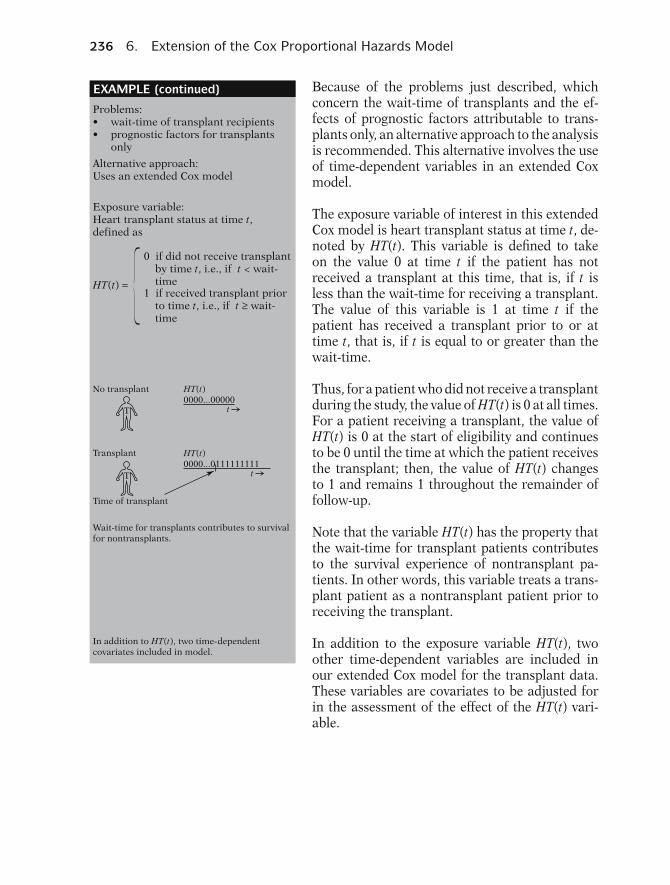
236 6. Extension of the Cox Proportional Hazards Model
EXAMPLE (continued)
HT(t) =
Problems:• wait-time of transplant recipients• prognostic factors for transplants
only
Alternative approach:Uses an extended Cox model
Exposure variable:Heart transplant status at time t,defined as
0 if did not receive transplant by time t, i.e., if t < wait- time
1 if received transplant prior to time t, i.e., if t ≥ wait- time
T
T
Wait-time for transplants contributes to survivalfor nontransplants.
In addition to HT(t), two time-dependentcovariates included in model.
No transplant
Transplant
Time of transplant
HT(t)0000...00000
t
t
HT(t)0000...0111111111
Because of the problems just described, whichconcern the wait-time of transplants and the ef-fects of prognostic factors attributable to trans-plants only, an alternative approach to the analysisis recommended. This alternative involves the useof time-dependent variables in an extended Coxmodel.
The exposure variable of interest in this extendedCox model is heart transplant status at time t, de-noted by HT(t). This variable is defined to takeon the value 0 at time t if the patient has notreceived a transplant at this time, that is, if t isless than the wait-time for receiving a transplant.The value of this variable is 1 at time t if thepatient has received a transplant prior to or attime t, that is, if t is equal to or greater than thewait-time.
Thus, for a patient who did not receive a transplantduring the study, the value of HT(t) is 0 at all times.For a patient receiving a transplant, the value ofHT(t) is 0 at the start of eligibility and continuesto be 0 until the time at which the patient receivesthe transplant; then, the value of HT(t) changesto 1 and remains 1 throughout the remainder offollow-up.
Note that the variable HT(t) has the property thatthe wait-time for transplant patients contributesto the survival experience of nontransplant pa-tients. In other words, this variable treats a trans-plant patient as a nontransplant patient prior toreceiving the transplant.
In addition to the exposure variable HT(t), twoother time-dependent variables are included inour extended Cox model for the transplant data.These variables are covariates to be adjusted forin the assessment of the effect of the HT(t) vari-able.

Presentation: VIII. The Analysis of the Stanford Heart Transplant Data 237
EXAMPLE (continued)
Note: HT(t) does not satisfy PHassumption.
Focus:Assessing the effect of HT(t) adjustedfor TMS(t) and AGE(t).
h(t,X(t)) = h0(t) exp[δ1HT(t)+ δ2TMS(t) + δ3AGE(t)]
VariableHT(t)TMS(t)AGE(t)
Coef.−3.17180.44420.0552
P>|z|0.0080.1120.014
Haz.Ratio0.04171.55931.0567
Std.Err.
1.18610.28020.0226
HR =ˆ
HR = e−3.1718 = 0.0417 =ˆ 123.98
124
h(transplants)
h(nontransplants)≈ ?
Not appropriate!
Covariates:
TMS(t) = 0 if t < wait-time TMS if t ≥ wait-time
AGE(t) = 0 if t < wait-time AGE if t ≥ wait-time
These covariates are denoted as TMS(t) andAGE(t) and they are defined as follows: TMS(t)equals 0 if t is less than the wait-time for a trans-plant but changes to the “tissue mismatch score”(TMS) at the time of the transplant if t is equalto or greater than the wait-time. Similarly, AGE(t)equals 0 if t is less than the wait-time but changesto AGE at time of transplant if t is equal to orgreater than the wait-time.
The extended Cox model for the transplant data isshown here. The model contains the three time-dependent variables HT(t), TMS(t) and AGE(t) asdescribed above.
For this model, since HT(t) is the exposure vari-able of interest, the focus of the analysis concernsassessing the effect of this variable adjusted forthe two covariates. Note, however, that becausethe HT(t) variable is time-dependent by definition,this variable does not satisfy the PH assumption,so that any hazard ratio estimate obtained for thisvariable is technically time-dependent.
A summary of computer results for the fit of theabove extended Cox model is shown here. Theseresults indicate that the exposure variable HT(t) issignificant below the one percent significance level(i.e., the two-sided p-value is 0.008). Thus, trans-plant status appears to be significantly associatedwith survival.
To evaluate the strength of the association, notethat e to the coefficient of HT(t) equals 0.0417.Since 1 over 0.0417 is 23.98, it appears that there isa 24-fold increase in the hazard of nontransplantpatients to transplant patients. The preceding in-terpretation of the value 0.0417 as a hazard ratioestimate is not appropriate, however, as we shallnow discuss further.

238 6. Extension of the Cox Proportional Hazards Model
EXAMPLE (continued)
ˆ23.98 is inappropriate as a HR:
Alternative interpretation:At time t,h (“not yet received transplant’’)≈ 24 h(“already received transplant’’)
More appropriate:
Hazard ratio formula should accountfor TMS and AGE.
Transplant? TMS(t)HT(t) AGE(t)
YesNo
10 0 0
TMS AGE
i denotes ith transplant patient
X*(t) = (HT(t) = 1, TMS(t) = TMSi, AGE(t) = AGEi)X(t) = (HT(t) = 0, TMS(t) = 0, AGE(t) = 0)
HR(t) = exp[δ1(1 − 0) + δ2(TMSi – 0)+ δ3(AGEi − 0)]= exp[δ1 + δ2TMSi + δ3AGEi]
= exp[−3.1718 + 0.4442 TMSi
+ 0.0552 AGEi]
• does not compare two separategroups
• exposure variable is not time-independent
• wait-time on transplants contributesto survival on nontransplants
First, note that the value of 23.98 inappropri-ately suggests that the hazard ratio is compar-ing two separate groups of patients. However, theexposure variable in this analysis is not a time-independent variable that distinguishes betweentwo separate groups. In contrast, the exposurevariable is time-dependent, and uses the wait-timeinformation on transplants as contributing to thesurvival experience of non-transplants.
Since the exposure variable is time-dependent, analternative interpretation of the hazard ratio esti-mate is that, at any given time t, the hazard for aperson who has not yet received a transplant (butmay receive one later) is approximately 24 timesthe hazard for a person who already has received atransplant by that time.
Actually, we suggest that a more appropriate haz-ard ratio expression is required to account fora transplant’s TMS and AGE score. Such an ex-pression would compare, at time t, the values ofeach of the three time-dependent variables in themodel. For a person who received a transplant,these values are 1 for HT(t) and TMS and AGE forthe two covariates. For a person who has not re-ceived a transplant, the values of all three variablesare 0.
Using this approach to compute the hazard ratio,the X∗(t) vector, which specifies the predictors fora patient i who received a transplant at time t, hasthe values 1, TMSi and AGEi for patient i; the X(t)vector, which specifies the predictors at time t fora patient who has not received a transplant at timet, has values of 0 for all three predictors.
The hazard ratio formula then reduces to e to thesum of δ1 “hat” plus δ2 “hat” times TMSi plus δ3“hat” times AGEi , where the δ “hat’s” are the es-timated coefficients of the three time-dependentvariables. Substituting the numerical values forthese coefficients in the formula gives the expo-nential expression circled here.

Presentation: IX. The Extended Cox Likelihood 239
EXAMPLE (continued)
HR(t) is time-dependent, i.e., its value at time t depends on TMSi and AGEi at time t
ˆ
TMS range: (0−3.05)AGE range: (12−64)
The resulting formula for the hazard ratio is time-dependent in that its value depends on the TMSand AGE values of the ith patient at the time oftransplant. That is, different patients can have dif-ferent values for TMS and AGE at time of trans-plant. Note that in the dataset, TMS ranged be-tween 0 and 3.05 and AGE ranged between 12 and64.
We end our discussion of the Stanford HeartTransplant Study at this point. For further insightinto the analysis of this dataset, we refer the readerto the 1977 paper by Crowley and Hu (J. Amer.Statist. Assoc.).
IX. The Extended CoxLikelihood
At the end of the presentation from Chapter 3 (Sec-tion VIII), we illustrated the Cox likelihood usingthe dataset shown on the left. In this section weextend that discussion to illustrate the Cox likeli-hood with a time-dependent variable.
To review: The data indicate that Barry got theevent at TIME = 2 years. Gary got the event at3 years, Harry was censored at 5 years, and Larrygot the event at 8 years. Furthermore, Barry andLarry were smokers whereas Gary and Harry werenonsmokers.
ID TIME STATUS SMOKE
Barry 2 1 1Gary 3 1 0Harry 5 0 0Larry 8 1 1
SURVT = Survival time (in years)STATUS = 1 for event, 0 forcensorshipSMOKE = 1 for a smoker, 0 for anonsmoker
Cox PH model: h(t) = h0(t)eβ1SMOKE In Chapter 3 we constructed the Cox likelihoodwith one predictor SMOKE in the model. Themodel and the likelihood are shown on the left.The likelihood is a product of three terms, oneterm for each event time tj (TIME = 2, 3, and 8).The denominator of each term is the sum of thehazards from the subjects still in the risk set attime tj, including the censored subject Harry. Thenumerator of each term is the hazard of the sub-ject who got the event at tj. The reader may wishto reread Section VIII of Chapter 3.
Cox PH Likelihood
L =[h0(t)eβ1
h0(t)eβ1 + h0(t)e0 + h0(t)e0 + h0(t)eβ1
]
×[
h0(t)e0
h0(t)e0 + h0(t)e0 + h0(t)eβ1
]
×[
h0(t)eβ1
h0(t)eβ1
]

240 6. Extension of the Cox Proportional Hazards Model
Cox extended model
h(t) = h0(t)eβ1SMOKE + β2SMOKE × TIME↗Time-dependent covariate(its value changes over time)
Now consider an extended Cox model, which con-tains the predictor SMOKE, and a time-dependentvariable SMOKE × TIME. For this model it is notonly the baseline hazard that may change overtime but also the value of the predictor variables.This can be illustrated by examining Larry’s haz-ard at each event time.
Larry got the event at TIME = 8
Larry’s hazard at each event time
TIME Larry’s Hazard
2 h0(t)eβ1+2β2
3 h0(t)eβ1+3β2
8 h0(t)eβ1+8β2
Larry, a smoker, got the event at TIME = 8.However at TIME = 2, 3, and 8, the covariateSMOKE × TIME changes values, thus affectingLarry’s hazard at each event time (see left). Un-derstanding how the expression for an individual’shazard changes over time is the key addition to-ward understanding how the Cox extended likeli-hood differs from the Cox PH likelihood.
Cox extended model
L =[h0(t)eβ1+2β2
h0(t)eβ1+2β2 + h0(t)e0 + h0(t)e0 + h0(t)eβ1+2β2
]
×[
h0(t)e0
h0(t)e0 + h0(t)e0 + h0(t)eβ1+3β2
]
×[
h0(t)eβ1+8β2
h0(t)eβ1+8β2
]
Likelihood is product of 3 terms:L = L1 × L2 × L3↗ ↑ ↖
Barry Gary Larry(t = 2) (t = 3) (t = 8)
The likelihood for the extended Cox model is con-structed in a similar manner to that of the likeli-hood for the Cox PH model. The difference is thatthe expression for the subject’s hazard is allowedto vary over time. The extended Cox likelihood forthese data is shown on the left.
Just as with the Cox PH likelihood shown previ-ously, the extended Cox likelihood is also a productof three terms, corresponding to the three eventtimes (L = L1 × L2 × L3). Barry got the eventfirst at t = 2, then Gary at t = 3, and finally Larryat t = 8. Harry, who was censored at t = 5, wasstill at risk when Barry and Gary got the event.Therefore, Harry’s hazard is still in the denomina-tor of L1 and L2.
SMOKE × TIME = 0 for nonsmok-ers
SMOKE × TIME changes over timefor smokers
Larry’s hazard changes over L1, L2,L3.
The inclusion of the time-varying covariateSMOKE × TIME does not change the expres-sion for the hazard for the nonsmokers (Gary andHarry) because SMOKE is coded 0 for nonsmok-ers. However, for smokers (Barry and Larry), theexpression for the hazard changes with time. No-tice how Larry’s hazard changes in the denomina-tor of L1, L2 and L3 (see dashed arrows above).

Presentation: IX. The Extended Cox Likelihood 241
h0(t) cancels in L
L =[
eβ1+2β2
eβ1+2β2 + e0 + e0 + eβ1+2β2
]×
[e0
e0 + e0 + eβ1+3β2
]×
[eβ1+8β2
eβ1+8β2
]
The baseline hazard cancels in the extended Coxlikelihood as it does with the Cox PH likelihood.Thus, the form of the baseline hazard need not bespecified, as it plays no role in the estimation ofthe regression parameters.
Incorrent coding of SMOKE × TIME
SMOKEID TIME STATUS SMOKE × TIME
Barry 2 1 1 2Gary 3 1 0 0Harry 5 0 0 0Larry 8 1 1 8↗
Coded as time-independent,not time-dependent
A word of caution for those planning to run amodel with a time-varying covariate: it is incor-rect to create a product term with TIME in thedata step by multiplying each individual’s valuefor SMOKE with his survival time. In other words,SMOKE × TIME should not be coded like the typ-ical interaction term. In fact, if SMOKE × TIMEwere coded as it is on the left, then SMOKE ×TIME would be a time-independent variable.Larry’s value for SMOKE × TIME is incorrectlycoded at a constant value of 8 even though Larry’svalue for SMOKE × TIME changes in the likeli-hood over L1, L2, and L3.
Incorrectly coded SMOKE × TIME
� Time independent� Probably highly significant� Survival time should predictsurvival time� But not meaningful
If the incorrectly coded time-independentSMOKE × TIME were included in a Cox model itwould not be surprising if the coefficient estimatewere highly significant even if the PH assumptionwere not violated. It would be expected that aproduct term with each individual’s survival timewould predict the outcome (his survival time),but it would not be meaningful. Nevertheless, thisis a common mistake.
Correctly coding SMOKE × TIME
� Time dependent� Computer packages allowdefinition in the analyticprocedure� See Computer Appendix fordetails
To obtain a correctly defined SMOKE × TIMEtime-dependent variable, computer packages typ-ically allow the variable to be defined within theanalytic procedure. See Computer Appendix tosee how time-dependent variables are defined inStata, SAS, and SPSS.
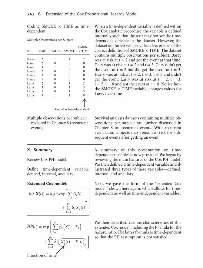
242 6. Extension of the Cox Proportional Hazards Model
Coding SMOKE × TIME as time-dependent
Multiple Observations per Subject
SMOKEID TIME STATUS SMOKE × TIME
Barry 2 1 1 2Gary 2 0 0 0Gary 3 1 0 0Harry 2 0 0 0Harry 3 0 0 0Harry 5 0 0 0Larry 2 0 1 2Larry 3 0 1 3Larry 5 0 1 5Larry 8 1 1 8↑
Coded as time-dependent
When a time-dependent variable is defined withinthe Cox analytic procedure, the variable is definedinternally such that the user may not see the time-dependent variable in the dataset. However, thedataset on the left will provide a clearer idea of thecorrect definition of SMOKE × TIME. The datasetcontains multiple observations per subject. Barrywas at risk at t = 2 and got the event at that time.Gary was at risk at t = 2 and t = 3. Gary didn’t getthe event at t = 2 but did get the event at t = 3.Harry was at risk at t = 2, t = 3, t = 5 and didn’tget the event. Larry was at risk at t = 2, t = 3,t = 5, t = 8 and got the event at t = 8. Notice howthe SMOKE × TIME variable changes values forLarry over time.
Multiple observations per subject:revisited in Chapter 8 (recurrentevents)
Survival analysis datasets containing multiple ob-servations per subject are further discussed inChapter 8 on recurrent events. With recurrentevent data, subjects may remain at risk for sub-sequent events after getting an event.
X. Summary A summary of this presentation on time-dependent variables is now provided. We began byreviewing the main features of the Cox PH model.We then defined a time-dependent variable and il-lustrated three types of these variables—defined,internal, and ancillary.
Review Cox PH model.
Define time-dependent variable:defined, internal, ancillary.
Extended Cox model:
h(t,X(t)) = h0(t) exp[ p1∑
i=1βi Xi
+p2∑
j=1δ j X j (t)
]Next, we gave the form of the “extended Coxmodel,” shown here again, which allows for time-dependent as well as time-independent variables.
HR(t) = exp
[p1∑
i=1
βi
[X ∗
i − Xi]
+p2∑
j=1
δ j[��
��X ∗
j (t) − X j (t)]]
↗Function of time
We then described various characteristics of thisextended Cox model, including the formula for thehazard ratio. The latter formula is time-dependentso that the PH assumption is not satisfied.

Presentation: X. Summary 243
Model for assessing PHassumption:
h(t,X(t)) = h0(t) exp[ p∑
i=1βi Xi
+p∑
i=1δi Xi gi (t)
]
We also showed how to use time-dependent vari-ables to assess the PH assumption for time-independent variables. A general formula for anextended Cox model that simultaneously consid-ers all time-independent variables of interest isshown here.
Examples of gi (t):t, log t, heaviside function
The functions gi (t) denote functions of time forthe ith variable that are to be determined by the in-vestigator. Examples of such functions are gi (t) =t, log t, or a heaviside function.
Heaviside functions:
HR
t
The use of heaviside functions were described andillustrated. Such functions allow for the hazardratio to be constant within different time intervals.
h(t,X(t)) = h0(t) exp[βE + δEg (t)]
where
g (t) ={
1 if t ≥ t00 if t < t0
h(t,X(t))= h0(t) exp[β1 Eg1(t) + β2 Eg2(t)]
where
g1(t) ={
1 if t ≥ t00 if t < t0
g2(t) ={
1 if t < t00 if t ≥ t0
For two time intervals, the model can take eitherone of two equivalent forms as shown here. Thefirst model contains a main effect of exposure andonly one heaviside function. The second modelcontains two heaviside functions without a maineffect of exposure. Both models yield two distinctand equivalent values for the hazard ratio.
EXAMPLE 1
1991 Australian study of heroin addicts
• two methadone maintenance clinics • addicts dataset file • clnic variable did not satisfy PH
assumption
We illustrated the use of time-dependent variablesthrough two examples. The first example consid-ered the comparison of two methadone mainte-nance clinics for heroin addicts. The dataset filewas called addicts. In this example, the clinic vari-able, which was a dichotomous exposure variable,did not satisfy the PH assumption.
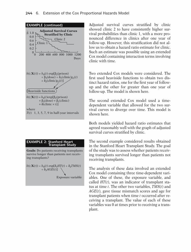
244 6. Extension of the Cox Proportional Hazards Model
EXAMPLE (continued)
h(t,X(t)) = h0(t)exp[β2(prison)+ β3(dose) + β1(clinic)+ δ(clinic × t)]
Adjusted Survival Curves Stratified by Clinic
Clinic 1Clinic 2
00
0.20.40.60.81.0
200 400 600 800 1000 1200Days
S
Heaviside functions
whereT(t) 1, 3, 5, 7, 9 in half-year intervals
h(t,X(t)) = h0(t) exp[β2(prison)+ β3(dose) + δ1(clinic)g1(t)+ δ2(clinic)g2(t)]
Adjusted survival curves stratified by clinicshowed clinic 2 to have consistently higher sur-vival probabilities than clinic 1, with a more pro-nounced difference in clinics after one year offollow-up. However, this stratification did not al-low us to obtain a hazard ratio estimate for clinic.Such an estimate was possible using an extendedCox model containing interaction terms involvingclinic with time.
Two extended Cox models were considered. Thefirst used heaviside functions to obtain two dis-tinct hazard ratios, one for the first year of follow-up and the other for greater than one year offollow-up. The model is shown here.
The second extended Cox model used a time-dependent variable that allowed for the two sur-vival curves to diverge over time. This model isshown here.
Both models yielded hazard ratio estimates thatagreed reasonably well with the graph of adjustedsurvival curves stratified by clinic.
EXAMPLE 2: Stanford Heart Transplant Study
h(t,X(t)) = h0(t) exp[δ1HT(t) + δ2TMS(t)+ δ3AGE(t)]
Goals: Do patients receiving transplants survive longer than patients not receiv- ing transplants?
Exposure variable
The second example considered results obtainedin the Stanford Heart Transplant Study. The goalof the study was to assess whether patients receiv-ing transplants survived longer than patients notreceiving transplants.
The analysis of these data involved an extendedCox model containing three time-dependent vari-ables. One of these, the exposure variable, andcalled HT(t), was an indicator of transplant sta-tus at time t. The other two variables, TMS(t) andAGE(t), gave tissue mismatch scores and age fortransplant patients when time t occurred after re-ceiving a transplant. The value of each of thesevariables was 0 at times prior to receiving a trans-plant.
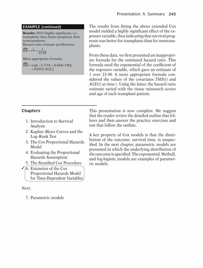
Presentation: X. Summary 245
EXAMPLE (continued)
HR = exp[ −3.1718 + 0.4442 TMSi+ 0.0552 AGEi]
ˆ
ˆ
Results: HT(t) highly significant, i.e., transplants have better prognosis than nontransplants.Hazard ratio estimate problematic:
HR = eδ1 = 123.98
More appropriate formula:
The results from fitting the above extended Coxmodel yielded a highly significant effect of the ex-posure variable, thus indicating that survival prog-nosis was better for transplants than for nontrans-plants.
From these data, we first presented an inappropri-ate formula for the estimated hazard ratio. Thisformula used the exponential of the coefficient ofthe exposure variable, which gave an estimate of1 over 23.98. A more appropriate formula con-sidered the values of the covariates TMS(t) andAGE(t) at time t. Using the latter, the hazard ratioestimate varied with the tissue mismatch scoresand age of each transplant patient.
Chapters This presentation is now complete. We suggestthat the reader review the detailed outline that fol-lows and then answer the practice exercises andtest that follow the outline.
A key property of Cox models is that the distri-bution of the outcome, survival time, is unspec-ified. In the next chapter, parametric models arepresented in which the underlying distribution ofthe outcome is specified. The exponential, Weibull,and log-logistic models are examples of paramet-ric models.
1. Introduction to SurvivalAnalysis
2. Kaplan–Meier Curves and theLog–Rank Test
3. The Cox Proportional HazardsModel
4. Evaluating the ProportionalHazards Assumption
5. The Stratified Cox Procedure✓ 6. Extension of the Cox
Proportional Hazards Modelfor Time-Dependent Variables
�
�
Next:
7. Parametric models

246 6. Extension of the Cox Proportional Hazards Model
DetailedOutline
I. Preview (page 214)II. Review of the Cox PH Model (pages 214–216)
A. The formula for the Cox PH model:
h(t,X) = h0(t) exp[ p∑
i=1βi Xi
]B. Formula for hazard ratio comparing two
individuals:
X∗ = (X ∗1, X ∗
2, . . . , X ∗p) and X = (X1, X2, . . . , X p) :
h(t,X∗)h(t,X)
= exp
[p∑
i=1
βi (X ∗i − Xi )
]
C. The meaning of the PH assumption:� Hazard ratio formula shows that the hazardratio is independent of time:
h(t,X∗)h(t,X)
= θ
� Hazard ratio for two X ’s are proportional:
h(t,X∗) = θh(t,X)
D. Three methods for checking the PH assumption:i. Graphical: Compare ln–ln survival curves or
observed versus predicted curvesii. Time-dependent covariates: Use product (i.e.,
interaction) terms of the form X × g (t).iii. Goodness-of-fit test: Use a large sample Z
statistic.E. Options when the PH assumption is not met:
i. Use a stratified Cox procedure.ii. Use an extended Cox model containing a
time-dependent variable of the form X × g (t).III. Definition and Examples of Time-Dependent
Variables (pages 216–219)A. Definition: any variable whose values differ over
timeB. Examples of defined, internal, and ancillary
time-dependent variables

Detailed Outline 247
IV. The Extended Cox Model for Time-DependentVaribles (pages 219–221)
A. h(t,X(t)) = h0(t) exp
[p1∑
i=1βi Xi +
p2∑j=1
δ j X j (t)
]
where X(t) = (X1, X2, . . . , X p1, X1(t), X2(t), . . . ,X p2 (t)) denotes the entire collection of predictorsat time t, Xi denotes the ith time-independentvariable, and X j (t) denotes the jth time-dependentvariable.
B. ML procedure used to estimate regressioncoefficients.
C. List of computer programs for the extended Coxmodel.
D. Model assumes that the hazard at time t dependson the value of X j (t) at the same time.
E. Can modify model for lag-time effect.V. The Hazard Ratio Formula for the Extended Cox
Model (pages 221–223)
A.
HR(t) = exp[ p1∑
i=1βi
[X ∗
i − Xi]
+p2∑
j=1δ j
[X ∗
j (t) − X j (t)]]
B. Because HR(t) is a function of time, the PHassumption is not satisfied.
C. The estimated coefficient of X j (t) istime-independent, and represents an “overall”effect of X j (t).
VI. Assessing Time-Independent Variables That DoNot Satisfy the PH Assumption (pages 224–229)A. General formula for assessing PH assumption:
h(t,X(t)) = h0(t) exp[ p∑
i=1βi Xi +
p∑i=1
δi Xi gi (t)]
B. gi (t) is a function of time corresponding to Xi
C. Test H0: δ1 = δ2 = . . . = δp = 0D. Heaviside function:
g (t) ={
1 if t ≥ t00 if t < t0

248 6. Extension of the Cox Proportional Hazards Model
E. The model with a single heaviside function:
h(t,X(t)) = h0(t) exp[βE + δEg (t)]
F. The model with two heaviside functions:
h(t,X(t)) = h0(t) exp[δ1 Eg1(t) + δ2 Eg2(t)]
where
g1(t) ={
1 if t ≥ t00 if t < t0
and g2(t) ={
1 if t < t00 if t ≥ t0
G. The hazard ratios:
t ≥ t0 : HR = exp(β + δ) = exp(δ1)
t < t0 : HR = exp(β) = exp(δ2)
H. Several heaviside functions: examples given withfour time-intervals:� Extended Cox model contains either
{E, E × g1(t), E × g2(t), E × g3(t)} or{E × g1(t), E × g2(t), E × g3(t), E × g4(t)}� The model using four product terms and nomain effect of E:
h(t,X(t)) = h0(t) exp[δ1 Eg1(t) + δ2 Eg2(t)+ δ3 Eg3(t) + δ4 Eg4(t)]
where
gi (t) ={
1 if t is within interval i0 if otherwise
VII. An Application of the Extended Cox Model to anEpidemiologic Study on the Treatment of HeroinAddiction (pages 230–234)A. 1991 Australian study of heroin addicts� two methadone maintenance clinics� addicts dataset file� clinic variable did not satisfy PH assumptionB. Clinic 2 has consistently higher retention
probabilities than clinic 1, with a morepronounced difference in clinics after one year oftreatment.
C. Two extended Cox models were considered:� Use heaviside functions to obtain two distincthazard ratios, one for less than one year and theother for greater than one year.� Use a time-dependent variable that allows forthe two survival curves to diverge over time.

Practice Exercises 249
VIII. An Application of the Extended Cox Model to theAnalysis of the Stanford Heart Transplant Data(pages 235–239)A. The goal of the study was to assess whether
patients receiving transplants survived longer thanpatients not receiving transplants.
B. We described an extended Cox model containingthree time-dependent variables:
h(t,X(t)) = h0(t) exp[δ1HT(t) + δ2TMS(t) + δ3AGE(t)]
C. The exposure variable, called HT(t), was anindicator of transplant status at time t. The othertwo variables, TMS(t) and AGE(t), gave tissuemismatch scores and age for transplant patientswhen time t occurred after receiving a transplant.
D. The results yielded a highly significant effect of theexposure variable.
E. The use of a hazard ratio estimate for this data wasproblematical.� An inappropriate formula is the exponential of
the coefficient of HT(t), which yields 1/23.98.� An alternative formula considers the values ofthe covariates TMS(t) and AGE(t) at time t.
IX. Extended Cox Likelihood (pages 239–242)A. Review of PH likelihood (Chapter 3).B. Barry, Gary, Larry, example of Cox likelihood.
X. Summary (pages 242–245)
PracticeExercises
The following dataset called “anderson.dat” consists of remis-sion survival times on 42 leukemia patients, half of whomreceive a new therapy and the other half of whom get a stan-dard therapy (Freireich et al., Blood, 1963). The exposure vari-able of interest is treatment status (Rx = 0 if new treatment,Rx = 1 if standard treatment). Two other variables for con-trol are log white blood cell count (i.e., log WBC) and sex.Failure status is defined by the relapse variable (0 if censored,1 if failure). The dataset is listed as follows:
Subj Surv Relapse Sex log WBC Rx
1 35 0 1 1.45 02 34 0 1 1.47 03 32 0 1 2.2 04 32 0 1 2.53 05 25 0 1 1.78 06 23 1 1 2.57 0
(Continued on next page)

250 6. Extension of the Cox Proportional Hazards Model
Subj Surv Relapse Sex log WBC Rx
7 22 1 1 2.32 08 20 0 1 2.01 09 19 0 0 2.05 0
10 17 0 0 2.16 011 16 1 1 3.6 012 13 1 0 2.88 013 11 0 0 2.6 014 10 0 0 2.7 015 10 1 0 2.96 016 9 0 0 2.8 017 7 1 0 4.43 018 6 0 0 3.2 019 6 1 0 2.31 020 6 1 1 4.06 021 6 1 0 3.28 022 23 1 1 1.97 123 22 1 0 2.73 124 17 1 0 2.95 125 15 1 0 2.3 126 12 1 0 1.5 127 12 1 0 3.06 128 11 1 0 3.49 129 11 1 0 2.12 130 8 1 0 3.52 131 8 1 0 3.05 132 8 1 0 2.32 133 8 1 1 3.26 134 5 1 1 3.49 135 5 1 0 3.97 136 4 1 1 4.36 137 4 1 1 2.42 138 3 1 1 4.01 139 2 1 1 4.91 140 2 1 1 4.48 141 1 1 1 2.8 142 1 1 1 5 1
The following edited printout gives computer results for fit-ting a Cox PH model containing the three predictives Rx, logWBC, and Sex.
Cox regression [95% Conf.Analysis time t: survt Coef. Std. Err. p > |z| Haz. Ratio Interval] P(PH)
Sex 0.263 0.449 0.558 1.301 0.539 3.139 0.042log WBC 1.594 0.330 0.000 4.922 2.578 9.397 0.714Rx 1.391 0.457 0.002 4.018 1.642 9.834 0.500
No. of subjecs = 42 Log likelihood = −72.109
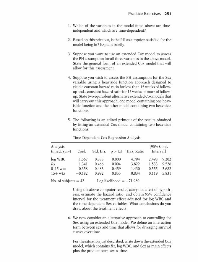
Practice Exercises 251
1. Which of the variables in the model fitted above are time-independent and which are time-dependent?
2. Based on this printout, is the PH assumption satisfied for themodel being fit? Explain briefly.
3. Suppose you want to use an extended Cox model to assessthe PH assumption for all three variables in the above model.State the general form of an extended Cox model that willallow for this assessment.
4. Suppose you wish to assess the PH assumption for the Sexvariable using a heaviside function approach designed toyield a constant hazard ratio for less than 15 weeks of follow-up and a constant hazard ratio for 15 weeks or more of follow-up. State two equivalent alternative extended Cox models thatwill carry out this approach, one model containing one heav-iside function and the other model containing two heavisidefunctions.
5. The following is an edited printout of the results obtainedby fitting an extended Cox model containing two heavisidefunctions:
Time-Dependent Cox Regression Analysis
Analysis [95% Conf.time t: survt Coef. Std. Err. p > |z| Haz. Ratio Interval]
log WBC 1.567 0.333 0.000 4.794 2.498 9.202Rx 1.341 0.466 0.004 3.822 1.533 9.5260–15 wks 0.358 0.483 0.459 1.430 0.555 3.68215+ wks −0.182 0.992 0.855 0.834 0.119 5.831
No. of subjects = 42 Log likelihood = −71.980
Using the above computer results, carry out a test of hypoth-esis, estimate the hazard ratio, and obtain 95% confidenceinterval for the treatment effect adjusted for log WBC andthe time-dependent Sex variables. What conclusions do youdraw about the treatment effect?
6. We now consider an alternative approach to controlling forSex using an extended Cox model. We define an interactionterm between sex and time that allows for diverging survivalcurves over time.
For the situation just described, write down the extended Coxmodel, which contains Rx, log WBC, and Sex as main effectsplus the product term sex × time.

252 6. Extension of the Cox Proportional Hazards Model
7. Using the model described in question 6, express the hazardratio for the effect of Sex adjusted for Rx and log WBC at 8and 16 weeks.
8. The following is an edited printout of computer resultsobtained by fitting the model described in question 6.
Time-Dependent Cox Regression Analysis
Analysis [95% Conf.time t: survt Coef. Std. Err. p > |z| Haz. Ratio Interval]
Sex 1.820 1.012 0.072 6.174 0.849 44.896log WBC 1.464 0.336 0.000 4.322 2.236 8.351Rx 1.093 0.479 0.022 2.984 1.167 7.626Sex × Time −0.345 0.199 0.083 0.708 0.479 1.046
No. of subjects = 42 Log likelihood = −70.416
Based on the above results, describe the hazard ratio estimatefor the treatment effect adjusted for the other variables in themodel, and summarize the results of the significance test andinterval estimate for this hazard ratio. How do these resultscompare with the results previously obtained when a heavi-side function approach was used? What does this comparisonsuggest about the drawbacks of using an extended Cox modelto adjust for variables not satisfying the PH assumption?
9. The following gives an edited printout of computer resultsusing a stratified Cox procedure that stratifies on the Sexvariable but keeps Rx and log WBC in the model.
Stratified Cox regression
Analysis [95% Conf.time t: survt Coef. Std. Err. p > |z| Haz. Ratio Interval]
log WBC 1.390 0.338 0.000 4.016 2.072 7.783Rx 0.931 0.472 0.048 2.537 1.006 6.396
No. of subjects = 42 Log likelihood = −57.560 Stratified by sex
Compare the results of the above printout with previouslyprovided results regarding the hazard ratio for the effect ofRx. Is there any way to determine which set of results is moreappropriate? Explain.

Test 253
Test The following questions consider the analysis of data from aclinical trial concerning gastric carcinoma, in which 90 pa-tients were randomized to either chemotherapy (coded as 2)alone or to a combination of chemotherapy and radiation(coded as 1). See Stablein et al., “Analysis of Survival Datawith Nonproportional Hazard Functions,” Controlled Clini-cal Trials, vol. 2, pp. 149–159 (1981). A listing of the dataset(called chemo) is given at the end of the presentation.
1. A plot of the log–log Kaplan–Meier curves for eachtreatment group is shown below. Based on this plot, whatwould you conclude about the PH assumption regardingthe treatment group variable? Explain.
2
22
22
2
11
11
11
12
0 200 400 600 800 1000 1200 1400
Log–log Survival Curves forEach Treatment Group
4.0
2.0
0.0
−2.0
Number at risk
45
45 40 25 17 10 7 6 2
26 20 11 10 7 5 2
2. The following is an edited printout of computer resultsobtained when fitting the PH model containing only thetreatment group variable. Based on these results, whatwould you conclude about the PH assumption regardingthe treatment group variable? Explain.
Cox regressionAnalysis time t: [95% Conf.survt Coef. Std. Err. p > |z| Haz. Ratio Interval] P(PH)
Tx −0.267 0.233 0.253 0.766 0.485 1.21 0
No. of subjects = 90 Log likelihood = −282.744
3. The following printout shows the results from using aheaviside function approach with an extended Cox modelto fit these data. The model used product terms of thetreatment variable (Tx) with each of three heaviside func-tions. The first product term (called Time1) involves aheaviside function for the period from 0 to 250 days,the second product term (i.e., Time2) involves the periodfrom 250 to 500 days, and the third product term (i.e.,Time3) involves the open-ended period from 500 days andbeyond.
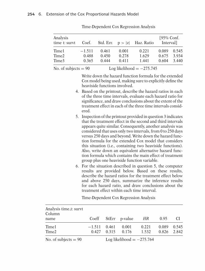
254 6. Extension of the Cox Proportional Hazards Model
Time-Dependent Cox Regression Analysis
Analysis [95% Conf.time t: survt Coef. Std. Err. p > |z| Haz. Ratio Interval]
Time1 −1.511 0.461 0.001 0.221 0.089 0.545Time2 0.488 0.450 0.278 1.629 0.675 3.934Time3 0.365 0.444 0.411 1.441 0.604 3.440
No. of subjects = 90 Log likelihood = −275.745
Write down the hazard function formula for the extendedCox model being used, making sure to explicitly define theheaviside functions involved.
4. Based on the printout, describe the hazard ratios in eachof the three time intervals, evaluate each hazard ratio forsignificance, and draw conclusions about the extent of thetreatment effect in each of the three time intervals consid-ered.
5. Inspection of the printout provided in question 3 indicatesthat the treatment effect in the second and third intervalsappears quite similar. Consequently, another analysis wasconsidered that uses only two intervals, from 0 to 250 daysversus 250 days and beyond. Write down the hazard func-tion formula for the extended Cox model that considersthis situation (i.e., containing two heaviside functions).Also, write down an equivalent alternative hazard func-tion formula which contains the main effect of treatmentgroup plus one heaviside function variable.
6. For the situation described in question 5, the computerresults are provided below. Based on these results,describe the hazard ratios for the treatment effect belowand above 250 days, summarize the inference resultsfor each hazard ratio, and draw conclusions about thetreatment effect within each time interval.
Time-Dependent Cox Regression Analysis
Analysis time t: survtColumnname Coeff StErr p-value HR 0.95 CI
Time1 −1.511 0.461 0.001 0.221 0.089 0.545Time2 0.427 0.315 0.176 1.532 0.826 2.842
No. of subjects = 90 Log likelihood = −275.764
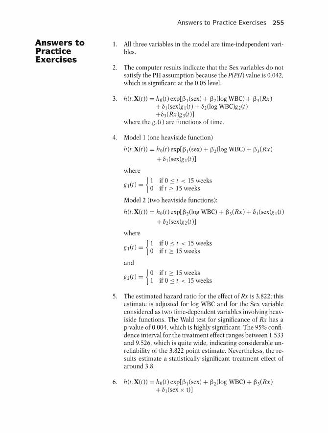
Answers to Practice Exercises 255
Answers toPracticeExercises
1. All three variables in the model are time-independent vari-bles.
2. The computer results indicate that the Sex variables do notsatisfy the PH assumption because the P(PH) value is 0.042,which is significant at the 0.05 level.
3. h(t,X(t)) = h0(t) exp[β1(sex) + β2(log WBC) + β3(Rx)+ δ1(sex)g1(t) + δ2(log WBC)g2(t)+δ3(Rx)g3(t)]
where the gi (t) are functions of time.
4. Model 1 (one heaviside function)
h(t,X(t)) = h0(t) exp[β1(sex) + β2(log WBC) + β3(Rx)
+ δ1(sex)g1(t)]
where
g1(t) ={
1 if 0 ≤ t < 15 weeks0 if t ≥ 15 weeks
Model 2 (two heaviside functions):
h(t,X(t)) = h0(t) exp[β2(log WBC) + β3(Rx) + δ1(sex)g1(t)
+ δ2(sex)g2(t)]
where
g1(t) ={
1 if 0 ≤ t < 15 weeks0 if t ≥ 15 weeks
and
g2(t) ={
0 if t ≥ 15 weeks1 if 0 ≤ t < 15 weeks
5. The estimated hazard ratio for the effect of Rx is 3.822; thisestimate is adjusted for log WBC and for the Sex variableconsidered as two time-dependent variables involving heav-iside functions. The Wald test for significance of Rx has ap-value of 0.004, which is highly significant. The 95% confi-dence interval for the treatment effect ranges between 1.533and 9.526, which is quite wide, indicating considerable un-reliability of the 3.822 point estimate. Nevertheless, the re-sults estimate a statistically significant treatment effect ofaround 3.8.
6. h(t,X(t)) = h0(t) exp[β1(sex) + β2(log WBC) + β3(Rx)+ δ1(sex × t)]

256 6. Extension of the Cox Proportional Hazards Model
7. The hazard ratio for the effect of Sex in each time interval,controlling for Rx and log WBC is given as follows:
t = 8 weeks HR = exp[β1 + 8δ1]t = 16 weeks HR = exp[β1 + 16δ1]
8. Using the model containing Sex, log WBC, Rx, and Sex ×Time, the estimated hazard ratio for the treatment effect isgiven by 2.984, with a p-value of 0.022 and a 95% confi-dence interval ranging between 1.167 and 7.626. The pointestimate of 2.984 is quite different from the point estimateof 3.822 for the heaviside function model, although the con-fidence intervals for both models are wide enough to in-clude both estimates. The discrepancy between point esti-mates demonstrates that when a time-dependent variableapproach is to be used to account for a variable not satis-fying the PH assumption, different results may be obtainedfrom different choices of time-dependent variables.
9. The stratified Cox analysis yields a hazard ratio of 2.537 witha p-value of 0.048 and a 95% CI ranging between 1.006 and6.396. The point estimate is much closer to the 2.984 forthe model containing the Sex × Time product term than tothe 3.822 for the model containing two heaviside functions.One way to choose between models would be to comparegoodness-of-fit test statistics for each model; another way isto compare graphs of the adjusted survival curves for eachmodel and determine by eye which set of survival curves fitsthe data better.

7 ParametricSurvivalModels
257

258 7. Parametric Survival Models
Introduction The Cox model is the most widely used survival model in thehealth sciences, but it is not the only model available. In thischapter we present a class of survival models, called paramet-ric models, in which the distribution of the outcome (i.e., thetime to event) is specified in terms of unknown parameters.Many parametric models are acceleration failure time modelsin which survival time is modeled as a function of predictorvariables. We examine the assumptions that underlie acceler-ated failure time models and compare the acceleration factoras an alternative measure of association to the hazard ratio.We present examples of the exponential, Weibull, and log-logistic models and give a brief description of other paramet-ric approaches. The parametric likelihood is constructed anddescribed in relation to left, right, and interval-censored data.Binary regression is presented as an alternative approach formodeling interval-censored outcomes. The chapter concludeswith a discussion of frailty models.
AbbreviatedOutline
The outline below gives the user a preview of the materialcovered by the presentation. A detailed outline for review pur-poses follows the presentation.
I. Overview (pages 260–262)II. Probability Density Function in Relation to the
Hazard and Survival Function (pages 262–263)III. Exponential Example (pages 263–265)IV. Accelerated Failure Time Assumption
(pages 266–268)V. Exponential Example Revisited (pages 268–272)
VI. Weibull Example (pages 272–277)VII. Log-Logistic Example (pages 277–282)
VIII. A More General Form of the AFT Model(pages 282–284)
IX. Other Parametric Models (pages 284–286)X. The Parametric Likelihood (pages 286–289)
XI. Interval-Censored Data (pages 289–294)XII. Frailty Models (pages 294–308)
XIII. Summary (pages 309–312)

Objectives 259
Objectives Upon completing this chapter, the learner should be able to:
1. State or recognize the form of a parametric survivalmodel and contrast it with a Cox model.
2. State common distributions used for parametric survivalmodels.
3. Contrast an AFT model with a PH model.4. Interpret output from an exponential survival model.5. Interpret output from a Weibull survival model.6. Interpret output from a log-logistic survival model.7. State or recognize the formulation of a parametric like-
lihood.8. State or recognize right-censored, left-censored, and
interval-censored data.9. State or recognize the form of a frailty model and the
purpose of including a frailty component.10. Interpret the output obtained from a frailty model.

260 7. Parametric Survival Models
Presentation
I. Overview In this chapter we present parametric survivalmodels and the assumptions that underlie thesemodels. Specifically we examine the acceleratedfailure time (AFT) assumption and contrast itto the proportional hazards (PH) assumption.We present examples of several parametric mod-els, including the exponential model, the Weibullmodel, and the log-logistic model. The paramet-ric likelihood is discussed and how it accommo-dates left-, right-, and interval-censored data. Wealso consider models that include a frailty com-ponent to account for unobserved heterogeneity.
parametric modelsexponential exampleAFT vs. PHWeibull examplelog-logistic exampleother approachesparametric likelihoodinterval-censoringfrailty models
Focus
Parametric Modeling
� Outcome assumed to followsome family of distributions� Exact distribution is unknownif parameters are unknown� Data used to estimateparameters� Examples of parametric models:◦ Linear regression◦ Logistic regression◦ Poisson regression
Linear regression, logistic regression, and Poissonregression are examples of parametric models thatare commonly used in the health sciences. Withthese models, the outcome is assumed to followsome distribution such as the normal, binomial,or Poisson distribution. Typically, what is actuallymeant is that the outcome follows some family ofdistributions of similar form with unknown pa-rameters. It is only when the value of the parame-ter(s) is known that the exact distribution is fullyspecified. For example, if one distribution is nor-mal with a mean of three and another distributionis normal with a mean of seven, the distributionsare of the same family (i.e., normal) but they arenot exactly the same distribution. For parametricregression models, the data are typically used toestimate the values of the parameters that fullyspecify that distribution.
Distributions commonly used forparametric survival models:
� Weibull� Exponential� Log-logistic� Lognormal� Generalized gamma
A parametric survival model is one in whichsurvival time (the outcome) is assumed to fol-low a known distribution. Examples of distribu-tions that are commonly used for survival timeare: the Weibull, the exponential (a special caseof the Weibull), the log-logistic, the lognormal,and the generalized gamma, all of which are sup-ported by SAS or Stata software.
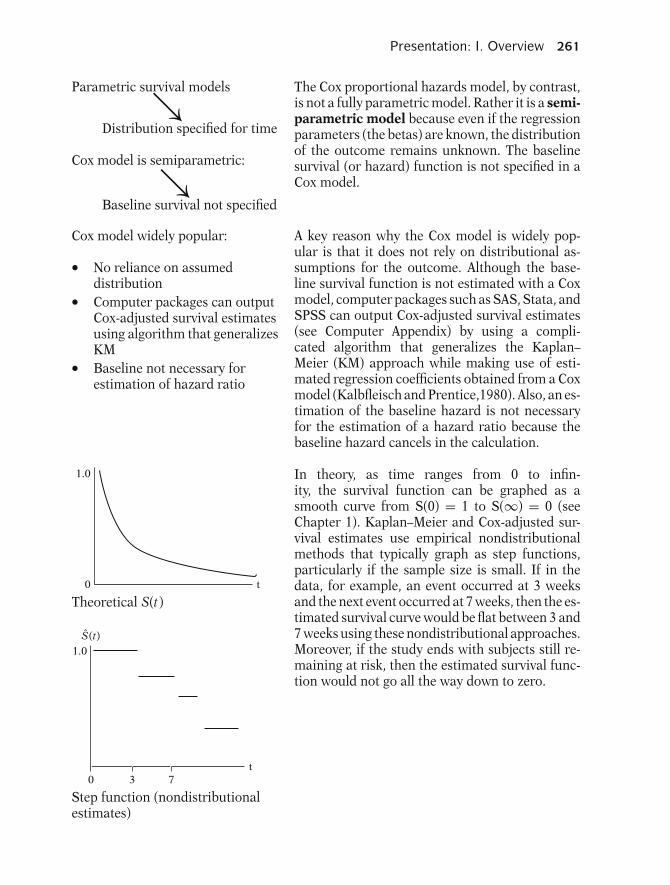
Presentation: I. Overview 261
Parametric survival models↘Distribution specified for time
Cox model is semiparametric:↘Baseline survival not specified
The Cox proportional hazards model, by contrast,is not a fully parametric model. Rather it is a semi-parametric model because even if the regressionparameters (the betas) are known, the distributionof the outcome remains unknown. The baselinesurvival (or hazard) function is not specified in aCox model.
Cox model widely popular:
� No reliance on assumeddistribution� Computer packages can outputCox-adjusted survival estimatesusing algorithm that generalizesKM� Baseline not necessary forestimation of hazard ratio
A key reason why the Cox model is widely pop-ular is that it does not rely on distributional as-sumptions for the outcome. Although the base-line survival function is not estimated with a Coxmodel, computer packages such as SAS, Stata, andSPSS can output Cox-adjusted survival estimates(see Computer Appendix) by using a compli-cated algorithm that generalizes the Kaplan–Meier (KM) approach while making use of esti-mated regression coefficients obtained from a Coxmodel (Kalbfleisch and Prentice,1980). Also, an es-timation of the baseline hazard is not necessaryfor the estimation of a hazard ratio because thebaseline hazard cancels in the calculation.
1.0
0 t
Theoretical S(t)
0 3 7
S(t)1.0
t
Step function (nondistributionalestimates)
In theory, as time ranges from 0 to infin-ity, the survival function can be graphed as asmooth curve from S(0) = 1 to S(∞) = 0 (seeChapter 1). Kaplan–Meier and Cox-adjusted sur-vival estimates use empirical nondistributionalmethods that typically graph as step functions,particularly if the sample size is small. If in thedata, for example, an event occurred at 3 weeksand the next event occurred at 7 weeks, then the es-timated survival curve would be flat between 3 and7 weeks using these nondistributional approaches.Moreover, if the study ends with subjects still re-maining at risk, then the estimated survival func-tion would not go all the way down to zero.
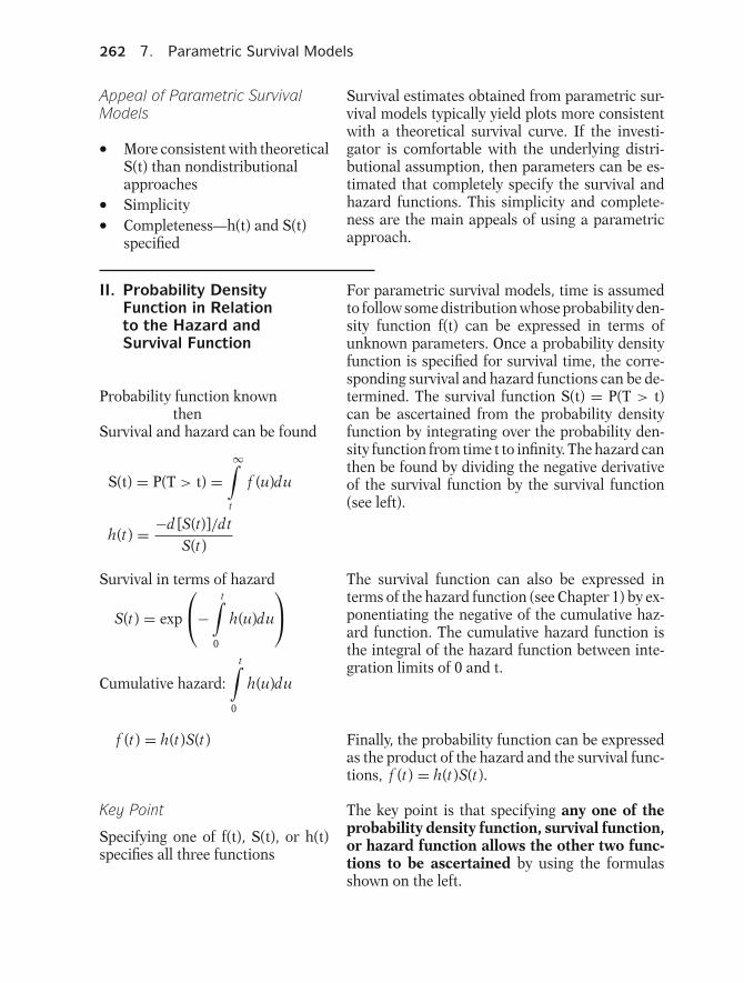
262 7. Parametric Survival Models
Appeal of Parametric SurvivalModels
� More consistent with theoreticalS(t) than nondistributionalapproaches� Simplicity� Completeness—h(t) and S(t)specified
Survival estimates obtained from parametric sur-vival models typically yield plots more consistentwith a theoretical survival curve. If the investi-gator is comfortable with the underlying distri-butional assumption, then parameters can be es-timated that completely specify the survival andhazard functions. This simplicity and complete-ness are the main appeals of using a parametricapproach.
II. Probability DensityFunction in Relationto the Hazard andSurvival Function
Probability function knownthen
Survival and hazard can be found
S(t) = P(T > t) =∞∫
t
f (u)du
h(t) = −d [S(t)]/dtS(t)
For parametric survival models, time is assumedto follow some distribution whose probability den-sity function f(t) can be expressed in terms ofunknown parameters. Once a probability densityfunction is specified for survival time, the corre-sponding survival and hazard functions can be de-termined. The survival function S(t) = P(T > t)can be ascertained from the probability densityfunction by integrating over the probability den-sity function from time t to infinity. The hazard canthen be found by dividing the negative derivativeof the survival function by the survival function(see left).
Survival in terms of hazard
S(t) = exp
⎛⎝−t∫
0
h(u)du
⎞⎠Cumulative hazard:
t∫0
h(u)du
The survival function can also be expressed interms of the hazard function (see Chapter 1) by ex-ponentiating the negative of the cumulative haz-ard function. The cumulative hazard function isthe integral of the hazard function between inte-gration limits of 0 and t.
f (t) = h(t)S(t) Finally, the probability function can be expressedas the product of the hazard and the survival func-tions, f (t) = h(t)S(t).
Key Point
Specifying one of f(t), S(t), or h(t)specifies all three functions
The key point is that specifying any one of theprobability density function, survival function,or hazard function allows the other two func-tions to be ascertained by using the formulasshown on the left.
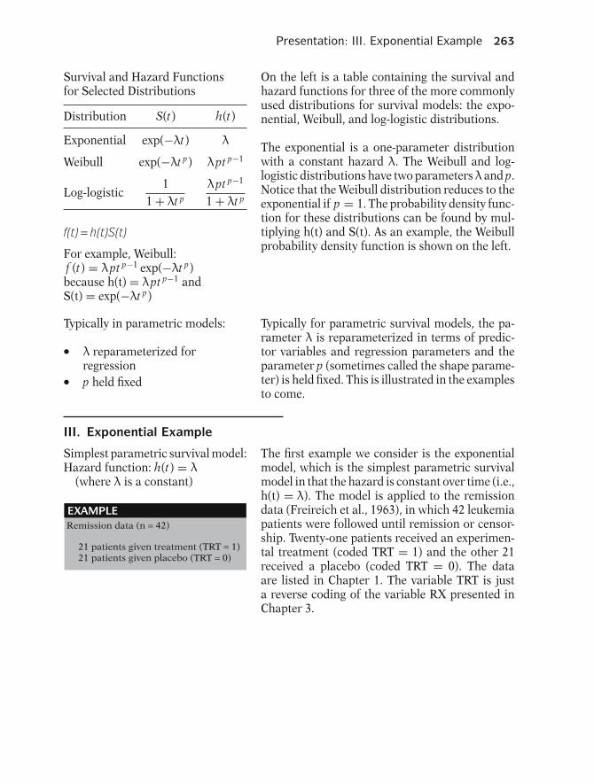
Presentation: III. Exponential Example 263
Survival and Hazard Functionsfor Selected Distributions
Distribution S(t) h(t)
Exponential exp(−λt) λ
Weibull exp(−λt p) λpt p−1
Log-logistic1
1 + λt p
λpt p−1
1 + λt p
On the left is a table containing the survival andhazard functions for three of the more commonlyused distributions for survival models: the expo-nential, Weibull, and log-logistic distributions.
The exponential is a one-parameter distributionwith a constant hazard λ. The Weibull and log-logistic distributions have two parameters λ and p.Notice that the Weibull distribution reduces to theexponential if p = 1. The probability density func-tion for these distributions can be found by mul-tiplying h(t) and S(t). As an example, the Weibullprobability density function is shown on the left.
f(t) = h(t)S(t)
For example, Weibull:f (t) = λpt p−1 exp(−λt p)because h(t) = λpt p−1 andS(t) = exp(−λt p)
Typically in parametric models:
� λ reparameterized forregression� p held fixed
Typically for parametric survival models, the pa-rameter λ is reparameterized in terms of predic-tor variables and regression parameters and theparameter p (sometimes called the shape parame-ter) is held fixed. This is illustrated in the examplesto come.
III. Exponential Example
Simplest parametric survival model:Hazard function: h(t) = λ
(where λ is a constant)
EXAMPLERemission data (n = 42)
21 patients given treatment (TRT = 1)21 patients given placebo (TRT = 0)
The first example we consider is the exponentialmodel, which is the simplest parametric survivalmodel in that the hazard is constant over time (i.e.,h(t) = λ). The model is applied to the remissiondata (Freireich et al., 1963), in which 42 leukemiapatients were followed until remission or censor-ship. Twenty-one patients received an experimen-tal treatment (coded TRT = 1) and the other 21received a placebo (coded TRT = 0). The dataare listed in Chapter 1. The variable TRT is justa reverse coding of the variable RX presented inChapter 3.
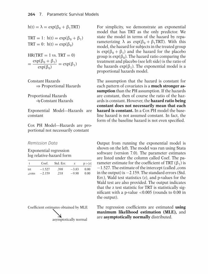
264 7. Parametric Survival Models
h(t) = λ = exp(β0 + β1TRT)
TRT = 1: h(t) = exp(β0 + β1)TRT = 0: h(t) = exp(β0)
HR(TRT = 1 vs. TRT = 0)
= exp(β0 + β1)exp(β0)
= exp(β1)
For simplicity, we demonstrate an exponentialmodel that has TRT as the only predictor. Westate the model in terms of the hazard by repa-rameterizing λ as exp(β0 + β1TRT). With thismodel, the hazard for subjects in the treated groupis exp(β0 + β1) and the hazard for the placebogroup is exp(β0). The hazard ratio comparing thetreatment and placebo (see left side) is the ratio ofthe hazards exp(β1). The exponential model is aproportional hazards model.
Constant Hazards⇒ Proportional Hazards
Proportional Hazards⇒\ Constant Hazards
Exponential Model—Hazards areconstant
Cox PH Model—Hazards are pro-portional not necessarily constant
The assumption that the hazard is constant foreach pattern of covariates is a much stronger as-sumption than the PH assumption. If the hazardsare constant, then of course the ratio of the haz-ards is constant. However, the hazard ratio beingconstant does not necessarily mean that eachhazard is constant. In a Cox PH model the base-line hazard is not assumed constant. In fact, theform of the baseline hazard is not even specified.
Remission Data
Exponential regressionlog relative-hazard form
t Coef. Std. Err. z p >|z|trt −1.527 .398 −3.83 0.00cons −2.159 .218 −9.90 0.00
Output from running the exponential model isshown on the left. The model was run using Statasoftware (version 7.0). The parameter estimatesare listed under the column called Coef. The pa-rameter estimate for the coefficient of TRT (β1) is−1.527. The estimate of the intercept (called consin the output) is −2.159. The standard errors (Std.Err.), Wald test statistics (z), and p-values for theWald test are also provided. The output indicatesthat the z test statistic for TRT is statistically sig-nificant with a p-value <0.005 (rounds to 0.00 inthe output).
Coefficient estimates obtained by MLE↘asymptotically normal
The regression coefficients are estimated usingmaximum likelihood estimation (MLE), andare asymptotically normally distributed.

Presentation: III. Exponential Example 265
TRT = 1: h (t) = exp(−2.159+ (−1.527)) = 0.025
TRT = 0: h (t) = exp(−2.159)= 0.115
HR (TRT = 1 vs. 0) = exp(−1.527)= 0.22
95% CI =exp[−1.527 ± 1.96(0.398)]= (0.10, 0.47)
Results: suggest treatment lowershazard
The estimated hazards for TRT = 1 and TRT =0 are shown on the left. The estimated hazardratio of 0.22 is obtained by exponentiating theestimated coefficient (−1.527) of the TRT vari-able. A 95% confidence interval can be calculatedexp[−1.527 ± 1.96(0.398)] yielding a CI of (0.10,0.47). These results suggest that the experimentaltreatment delays remission.
Parametric models
� Need not be PH models� Many are AFT models
Exponential and Weibull
� Accommodate PH and AFTassumptions
Up to this point in the book, the key assump-tion for survival models has been the proportionalhazard assumption. However, parametric survivalmodels need not be PH models. Many paramet-ric models are acceleration failure time mod-els rather than PH models. The exponential andWeibull distributions can accommodate both thePH and AFT assumptions.
Remission Data
Exponential regressionaccelerated failure-time form
t Coef. Std. Err. z p >|z|trt 1.527 .398 3.83 0.00cons 2.159 .218 9.90 0.00
On the left is Stata output from the AFT form ofthe exponential model with TRT as the only pre-dictor. Stata can output both the PH or AFT formof an exponential or Weibull model (see ComputerAppendix). SAS (version 8.2) only runs the AFTform of parametric models and SPSS (version11.5) does not yet provide commands to run para-metric models.
AFT vs. PH
� Different interpretation ofparameters� AFT applies to comparison ofsurvival times� PH applies to comparison ofhazards
The interpretation of parameters differs for AFTand PH models. The AFT assumption is applicablefor a comparison of survival times whereas thePH assumption is applicable for a comparison ofhazards. In the following sections we discuss theAFT assumption and then revisit this example anddiscuss the AFT form of this model.
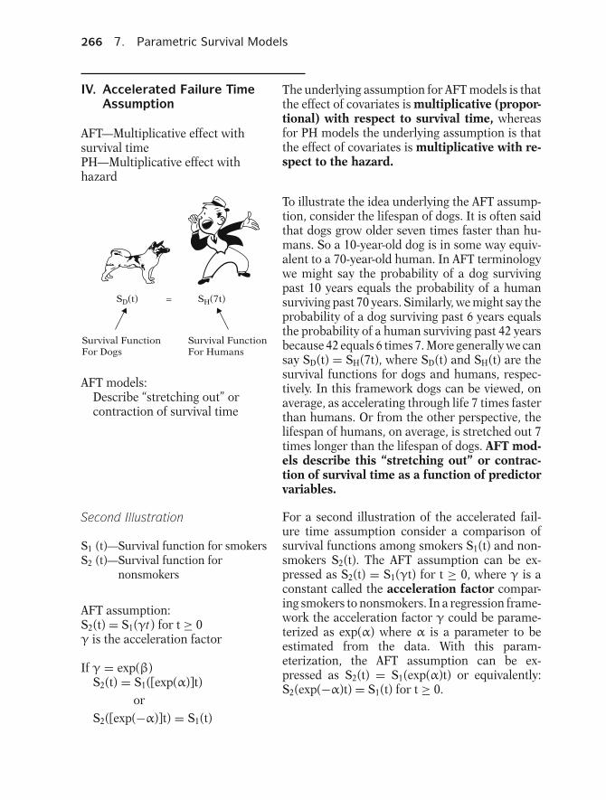
266 7. Parametric Survival Models
IV. Accelerated Failure TimeAssumption
The underlying assumption for AFT models is thatthe effect of covariates is multiplicative (propor-tional) with respect to survival time, whereasfor PH models the underlying assumption is thatthe effect of covariates is multiplicative with re-spect to the hazard.
AFT—Multiplicative effect withsurvival timePH—Multiplicative effect withhazard
SD(t) SH(7t)=
Survival FunctionFor Dogs
Survival FunctionFor Humans
AFT models:Describe “stretching out” orcontraction of survival time
To illustrate the idea underlying the AFT assump-tion, consider the lifespan of dogs. It is often saidthat dogs grow older seven times faster than hu-mans. So a 10-year-old dog is in some way equiv-alent to a 70-year-old human. In AFT terminologywe might say the probability of a dog survivingpast 10 years equals the probability of a humansurviving past 70 years. Similarly, we might say theprobability of a dog surviving past 6 years equalsthe probability of a human surviving past 42 yearsbecause 42 equals 6 times 7. More generally we cansay SD(t) = SH(7t), where SD(t) and SH(t) are thesurvival functions for dogs and humans, respec-tively. In this framework dogs can be viewed, onaverage, as accelerating through life 7 times fasterthan humans. Or from the other perspective, thelifespan of humans, on average, is stretched out 7times longer than the lifespan of dogs. AFT mod-els describe this “stretching out” or contrac-tion of survival time as a function of predictorvariables.
Second Illustration
S1 (t)—Survival function for smokersS2 (t)—Survival function for
nonsmokers
AFT assumption:S2(t) = S1(γt) for t ≥ 0γ is the acceleration factor
If γ = exp(β)S2(t) = S1([exp(α)]t)
orS2([exp(−α)]t) = S1(t)
For a second illustration of the accelerated fail-ure time assumption consider a comparison ofsurvival functions among smokers S1(t) and non-smokers S2(t). The AFT assumption can be ex-pressed as S2(t) = S1(γt) for t ≥ 0, where γ is aconstant called the acceleration factor compar-ing smokers to nonsmokers. In a regression frame-work the acceleration factor γ could be parame-terized as exp(α) where α is a parameter to beestimated from the data. With this param-eterization, the AFT assumption can be ex-pressed as S2(t) = S1(exp(α)t) or equivalently:S2(exp(−α)t) = S1(t) for t ≥ 0.

Presentation: IV. Accelerated Failure Time Assumption 267
Suppose exp(α) = 0.75thenS2(80) = S1(60)S2(40) = S1(30)
More generallyS2(t) = S1(0.75t)
Suppose exp(α) = 0.75; then the probability of anonsmoker surviving 80 years equals the proba-bility of a smoker surviving 80(0.75) or 60 years.Similarly, the probability of a nonsmoker surviv-ing 40 years equals the probability of a smokersurviving 30 years. More generally, the probabilityof a nonsmoker surviving t years equals the proba-bility of a smoker surviving 0.75 times t years (i.e.,S2(t) = S1(0.75t)).
T1—Survival time for smokersT2—Survival time for nonsmokers
AFT assumption in terms of randomvariables:
T1 = γT2
The AFT assumption can also be expressed interms of random variables for survival time ratherthan the survival function. If T2 is a random vari-able (following some distribution) representingthe survival time for nonsmokers and T1 is a ran-dom variable representing the survival time forsmokers, then the AFT assumption can be ex-pressed as T1 = γ T2.
Acceleration factorMeasure of associationon survival time
Hazard ratioMeasure of association on thehazard
The acceleration factor is the key measure of as-sociation obtained in an AFT model. It allows theinvestigator to evaluate the effect of predictor vari-ables on survival time just as the hazard ratio al-lows the evaluation of predictor variables on thehazard.
Acceleration factor (γ)� Describes stretching orcontraction of S(t)� Ratio of times to any fixedvalue of S(t)
Suppose γ = 2.0(Group 2 vs. Group 1)� Time to S(t) = 0.50 (median) is
double for Group 2� Time to S(t) = 0.20 is double forGroup 2� Time to S(t) = 0.83 is double forGroup 2� Time to S(t) = 0.98 is double forGroup 2� Time to S(t) = q is double forGroup 2 (generalization)
The acceleration factor describes the “stretchingout” or contraction of survival functions whencomparing one group to another. More precisely,the acceleration factor is a ratio of survivaltimes corresponding to any fixed value of S(t).For example, if the acceleration factor comparingsubjects in Group 2 vs. Group 1 is γ = 2.0, thenthe median survival time (value of t when S(t) =0.5) for Group 2 is double the median survival timefor Group 1. Moreover, the time it takes for S(t) toequal 0.2 or 0.83 or 0.98 is double for Group 2compared to Group 1 for the same value of S(t).In general, the acceleration factor is a ratio of sur-vival times corresponding to any quantile of sur-vival time (S(t) = q).

268 7. Parametric Survival Models
1.00
0.75
0.50
0.25
S(t)
G = 1 G = 2t
γ = 2
distance to G = 1
distance to G = 2
Survival curves for Group 1 (G = 1)and Group 2 (G = 2)
Horizontal lines are twice as long toG = 2 compared to G = 1 becauseγ = 2
This idea is graphically illustrated by examiningthe survival curves for Group 1 (G = 1) and Group2 (G = 2) shown on the left. For any fixed value ofS(t), the distance of the horizontal line from theS(t) axis to the survival curve for G = 2 is doublethe distance to the survival curve for G = 1. No-tice the median survival time (as well as the 25thand 75th percentiles) is double for G = 2. For AFTmodels, this ratio of survival times is assumed con-stant for all fixed values of S(t).
V. Exponential ExampleRevisited
Remission data (n = 42)
21 patients given treatment (TRT = 1)21 patients given placebo (TRT = 0)
Previously discussed PH form ofmodelNow discuss AFT form of model
We return to the exponential example applied tothe remission data with treatment status (TRT) asthe only predictor. In Section III, results from thePH form of the exponential model were discussed.In this section we discuss the AFT form of themodel.
Exponential survival and hazardfunctions:
S(t) = exp(−λt)h(t) = λ
Recall for PH model:
h(t) = λ = exp(β0 + β1 TRT)
The exponential survival and hazard functions areshown on the left. Recall that the exponential haz-ard is constant and can be reparameterized as aPH model, h(t) = λ = exp(β0 + β1TRT). In thissection we show how S(t) can be reparameterizedas an AFT model.

Presentation: V. Exponential Example Revisited 269
AFT assumption(comparing 2 levels)
� Ratio of times is constant to allfixed S(t)
Strategy for developing the model:
� Solve for t in terms of S(t)� Scale t in terms of the predictors
The underlying AFT assumption, for comparingtwo levels of covariates, is that the ratio of timesto any fixed value of S(t) = q is constant for anyprobability q. We develop the model with the sur-vival function and solve for t in terms of S(t). Wethen scale t in terms of the predictors.
S(t) = exp(−λt)
t = [−ln(S(t)] × 1λ
let1λ
= exp(α0 + α1TRT)
t = [−ln(S(t)] × exp(α0 + α1TRT)
↗Scaling of t
Median survival time, S(t) = 0.5:
tm = [−ln(0.5)] × exp(α0 +α1TRT)
The exponential survival function is S(t) =exp(−λt). By solving for t, we can obtain a for-mula for t in terms of S(t). Taking the naturallog, multiplying by negative 1, and then multi-plying by the reciprocal of λ, yields the expres-sion for t shown on the left. By reparameteriz-ing 1/λ = exp(α0 + α1TRT), or equivalently λ =exp[−(α0 + α1TRT)], it can be seen how the pre-dictor variable TRT is used to scale the time toany fixed value of S(t) (see left). For example, tofind an expression for the median survival time tm,substitute S(t) = 0.5 (see left).
Let S(t) = qt = [−ln(q)] × exp(α0 + α1TRT)
Acceleration Factor:γ (TRT = 1 vs. TRT = 0)
γ = [−ln(q)] exp(α0 + α1)[−ln(q)] exp(α0)
= exp(α1)
The expression for t is restated on the left in termsof any fixed probability S(t) = q. The accelerationfactor γ is found by taking the ratio of the times toS(t) = q for TRT = 1 and TRT = 0. After canceling,γ reduces to exp(α1).
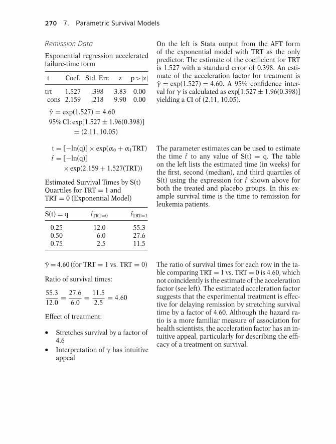
270 7. Parametric Survival Models
Remission Data
Exponential regression acceleratedfailure-time form
t Coef. Std. Err. z p >|z|trt 1.527 .398 3.83 0.00cons 2.159 .218 9.90 0.00
γ = exp(1.527) = 4.6095% CI: exp[1.527 ± 1.96(0.398)]
= (2.11, 10.05)
On the left is Stata output from the AFT formof the exponential model with TRT as the onlypredictor. The estimate of the coefficient for TRTis 1.527 with a standard error of 0.398. An esti-mate of the acceleration factor for treatment isγ = exp(1.527) = 4.60. A 95% confidence inter-val for γ is calculated as exp[1.527 ± 1.96(0.398)]yielding a CI of (2.11, 10.05).
t = [−ln(q)] × exp(α0 + α1TRT)t = [−ln(q)]
× exp(2.159 + 1.527(TRT))
Estimated Survival Times by S(t)Quartiles for TRT = 1 andTRT = 0 (Exponential Model)
S(t) = q tTRT=0 tTRT=1
0.25 12.0 55.30.50 6.0 27.60.75 2.5 11.5
The parameter estimates can be used to estimatethe time t to any value of S(t) = q. The tableon the left lists the estimated time (in weeks) forthe first, second (median), and third quartiles ofS(t) using the expression for t shown above forboth the treated and placebo groups. In this ex-ample survival time is the time to remission forleukemia patients.
γ= 4.60 (for TRT = 1 vs. TRT = 0)
Ratio of survival times:
55.312.0
= 27.66.0
= 11.52.5
= 4.60
Effect of treatment:
� Stretches survival by a factor of4.6� Interpretation of γ has intuitiveappeal
The ratio of survival times for each row in the ta-ble comparing TRT = 1 vs. TRT = 0 is 4.60, whichnot coincidently is the estimate of the accelerationfactor (see left). The estimated acceleration factorsuggests that the experimental treatment is effec-tive for delaying remission by stretching survivaltime by a factor of 4.60. Although the hazard ra-tio is a more familiar measure of association forhealth scientists, the acceleration factor has an in-tuitive appeal, particularly for describing the effi-cacy of a treatment on survival.

Presentation: V. Exponential Example Revisited 271
HR and γ are reciprocals in expo-nential models:
HR(TRT = 1 vs. 0) = exp(−1.527)= 0.22
γ(TRT = 1 vs. 0) = exp(1.527)= 4.60
In generalγ > 1 ⇒ exposure benefitssurvivalHR > 1 ⇒ exposure harmful tosurvival
γ < 1 ⇒ exposure harmful tosurvivalHR < 1 ⇒ exposure benefitssurvival
γ = HR = 1 ⇒ no effect fromexposure
Recall from Section III that the hazard ratiofor the effect of treatment was estimated atexp(−1.527) = 0.22 using the PH form of the ex-ponential model. This result illustrates a key prop-erty of the exponential model: the correspondingacceleration factor and hazards ratio (e.g., TRT =1 vs. TRT = 0) are reciprocals of each other. Thisproperty is unique to the exponential model. Whatcan be generalized, however, is that an accelera-tion factor greater than one for the effect of anexposure implies that the exposure is benefi-cial to survival whereas a hazard ratio greaterthan one implies the exposure is harmful tosurvival (and vice versa).
Exponential PH and AFT models:
� Same model� Different parameterization� Same estimates for◦ Survival function◦ Hazard function◦ Median survival
Although the exponential PH and AFT models fo-cus on different underlying assumptions, they arein fact the same model. The only difference isin their parameterization. The resulting estimatesfor the survival function, hazard function, and me-dian survival do not differ between these models(see Practice Exercises 6 and 7).

272 7. Parametric Survival Models
For those experienced with Poissonregression:
Exponential and Poisson models
� Assume a constant rate� Different data structure◦ Poisson—aggregate counts◦ Exponential—individual
level� Use different outcomes◦ Poisson—number of cases◦ Exponential—time to
event� Yield equivalent parameterestimates◦ With same data and same
covariates in the model
For those who have experience with Poisson re-gression, there is a close connection between theexponential and Poisson models. Both distribu-tions assume an underlying constant rate. In fact,if the data are structured such that all the casesand the total time at risk are aggregated for eachpattern of covariates (e.g., TRT = 1 and TRT = 0)and the log of the corresponding person-time atrisk is used as an offset, then a Poisson model willyield equivalent parameter estimates as the expo-nential PH model. The difference is that the ran-dom outcome for the Poisson model is the countof events over a fixed amount of time at risk andthe random outcome for the exponential model isthe time (at risk) to event.
Exponential model is special caseof Weibull model
We continue with the remission data example andpresent the more general Weibull model, whichincludes the exponential model as a special case.In the next section we also show a graphical ap-proach for evaluating the appropriateness of theWeibull (and thus also the exponential) model.
VI. Weibull Example
Weibull Model:
Hazard function: h(t) = λpt p−1
(where p > 0 and λ > 0)
p is a shape parameter
� p > 1 hazard increases overtime� p = 1 constant hazard(exponential model)� p < 1 hazard decreases overtime
Additional shape parameter offersgreater flexibility
The Weibull model is the most widely usedparametric survival model. Its hazard function ish(t) = λpt p−1, where p and λ > 0. As with the ex-ponential model, λ will be reparameterized withregression coefficients. The additional parameterp is called a shape parameter and determines theshape of the hazard function. If p > 1 then thehazard increases as time increases. If p = 1 thenthe hazard is constant and the Weibull model re-duces to the exponential model (h(t) = λ). If p < 1then the hazard decreases over time. The additionof this shape parameter gives the Weibull modelgreater flexibility than the exponential model yetthe hazard function remains relatively simple (ba-sically a scaling of t raised to some fixed power).
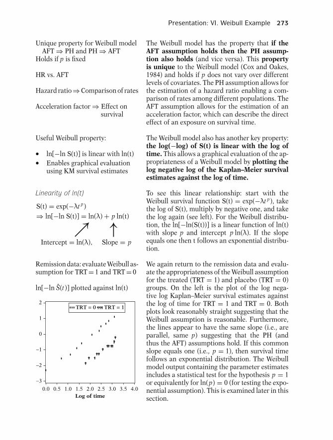
Presentation: VI. Weibull Example 273
Unique property for Weibull modelAFT ⇒ PH and PH ⇒ AFT
Holds if p is fixed
HR vs. AFT
Hazard ratio ⇒ Comparison of rates
Acceleration factor ⇒ Effect onsurvival
The Weibull model has the property that if theAFT assumption holds then the PH assump-tion also holds (and vice versa). This propertyis unique to the Weibull model (Cox and Oakes,1984) and holds if p does not vary over differentlevels of covariates. The PH assumption allows forthe estimation of a hazard ratio enabling a com-parison of rates among different populations. TheAFT assumption allows for the estimation of anacceleration factor, which can describe the directeffect of an exposure on survival time.
Useful Weibull property:
� ln[−ln S(t)] is linear with ln(t)� Enables graphical evaluationusing KM survival estimates
The Weibull model also has another key property:the log(−log) of S(t) is linear with the log oftime. This allows a graphical evaluation of the ap-propriateness of a Weibull model by plotting thelog negative log of the Kaplan–Meier survivalestimates against the log of time.
Linearity of ln(t)
S(t) = exp(−λt p)⇒ ln[−ln S(t)] = ln(λ) + p ln(t)
↗ ↑Intercept = ln(λ), Slope = p
To see this linear relationship: start with theWeibull survival function S(t) = exp(−λt p), takethe log of S(t), multiply by negative one, and takethe log again (see left). For the Weibull distribu-tion, the ln[−ln(S(t))] is a linear function of ln(t)with slope p and intercept p ln(λ). If the slopeequals one then t follows an exponential distribu-tion.
Remission data: evaluate Weibull as-sumption for TRT = 1 and TRT = 0
ln[−ln S(t)] plotted against ln(t)
0.0 0.5 1.0 1.5 2.0 2.5 3.0 3.5 4.0
−3
−2
−1
0
1
2TRT = 0 TRT = 1
Log of time
We again return to the remission data and evalu-ate the appropriateness of the Weibull assumptionfor the treated (TRT = 1) and placebo (TRT = 0)groups. On the left is the plot of the log nega-tive log Kaplan–Meier survival estimates againstthe log of time for TRT = 1 and TRT = 0. Bothplots look reasonably straight suggesting that theWeibull assumption is reasonable. Furthermore,the lines appear to have the same slope (i.e., areparallel, same p) suggesting that the PH (andthus the AFT) assumptions hold. If this commonslope equals one (i.e., p = 1), then survival timefollows an exponential distribution. The Weibullmodel output containing the parameter estimatesincludes a statistical test for the hypothesis p = 1or equivalently for ln(p) = 0 (for testing the expo-nential assumption). This is examined later in thissection.

274 7. Parametric Survival Models
Summary of possible results for plotof ln[−ln S(t)] against ln(t)
1. Parallel straight lines ⇒ Weibull,PH, and AFT assumptions hold
2. Parallel straight lines with slopeof 1 ⇒ Exponential. PH and AFT
3. Parallel but not straight lines ⇒PH but not Weibull, not AFT (canuse Cox model)
4. Not parallel and not straight ⇒Not Weibull, PH violated
5. Not parallel but straight lines ⇒Weibull holds, but PH and AFTviolated, different p
On the left is a summary of five possible re-sults from an examination of the log negative logKaplan–Meier survival estimates plotted againstthe log of time for two or more levels of covariates.The key points are that straight lines support theWeibull assumption and parallel curves sup-port the PH assumption. If the plots are parallelbut not straight then the PH assumption holds butnot the Weibull. Assessing whether the curves areparallel is a familiar approach for evaluating thePH assumption in a Cox model (see Chapter 4 andComputer Appendix). An interesting scenario oc-curs if the lines are straight but not parallel. In thissituation the Weibull assumption is supported butthe PH and AFT assumptions are violated. If thelines are not parallel, then p is not constant acrosslevels of covariates. In Section IX of this chapter,we present a method for modeling the shape pa-rameter p as a function of predictor variables, buttypically p is assumed fixed.
Previous plot suggests Weibull andPH assumption reasonable for TRT
An examination of the plot on the previous pagesuggests that the Weibull and PH assumptions arereasonable for treatment (TRT). First the PH formof the model is presented and then the AFT form.
Weibull PH model:
h(t) = λpt p−1
where λ = exp(β0 + β1TRT).
Hazard ratio (TRT = 1 vs. TRT = 0)
HR = exp(β0 + β1)pt p−1
exp(β0)pt p−1
= exp(β1)
The Weibull hazard function is h(t) = λpt p−1. AWeibull PH model is defined by reparameterizinglambda λ as exp(β0 + β1TRT). The hazard ratiois obtained by substituting TRT = 1 and TRT = 0into the hazard functions (see left). After cancelingwe obtain the familiar result exp(β1). Note thatthis result depends on p having the same value forTRT = 1 and TRT = 0, otherwise time (t) wouldnot cancel in the expression for the HR (i.e., PHassumption not satisfied).
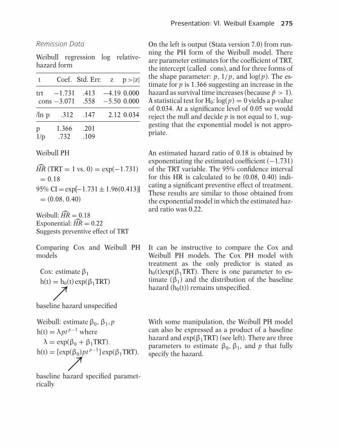
Presentation: VI. Weibull Example 275
Remission Data
Weibull regression log relative-hazard form
t Coef. Std. Err. z p >|z|trt −1.731 .413 −4.19 0.000cons −3.071 .558 −5.50 0.000
/ln p .312 .147 2.12 0.034
p 1.366 .2011/p .732 .109
On the left is output (Stata version 7.0) from run-ning the PH form of the Weibull model. Thereare parameter estimates for the coefficient of TRT,the intercept (called cons), and for three forms ofthe shape parameter: p, 1/p, and log(p). The es-timate for p is 1.366 suggesting an increase in thehazard as survival time increases (because p > 1).A statistical test for H0: log(p) = 0 yields a p-valueof 0.034. At a significance level of 0.05 we wouldreject the null and decide p is not equal to 1, sug-gesting that the exponential model is not appro-priate.
Weibull PH
HR (TRT = 1 vs. 0) = exp(−1.731)= 0.18
95% CI = exp[−1.731 ± 1.96(0.413)]= (0.08, 0.40)
Weibull: HR = 0.18Exponential: HR = 0.22Suggests preventive effect of TRT
An estimated hazard ratio of 0.18 is obtained byexponentiating the estimated coefficient (−1.731)of the TRT variable. The 95% confidence intervalfor this HR is calculated to be (0.08, 0.40) indi-cating a significant preventive effect of treatment.These results are similar to those obtained fromthe exponential model in which the estimated haz-ard ratio was 0.22.
Comparing Cox and Weibull PHmodels
Cox: estimate β1
h(t) = h0(t) exp(β1TRT)↗baseline hazard unspecified
Weibull: estimate β0,β1,ph(t) = λpt p−1 where
λ = exp(β0 + β1TRT).h(t) = [exp(β0)pt p−1] exp(β1TRT).↗baseline hazard specified paramet-rically
It can be instructive to compare the Cox andWeibull PH models. The Cox PH model withtreatment as the only predictor is stated ash0(t)exp(β1TRT). There is one parameter to es-timate (β1) and the distribution of the baselinehazard (h0(t)) remains unspecified.
With some manipulation, the Weibull PH modelcan also be expressed as a product of a baselinehazard and exp(β1TRT) (see left). There are threeparameters to estimate β0,β1, and p that fullyspecify the hazard.

276 7. Parametric Survival Models
S(t) = exp(−λt p)
solve for t
t = [−ln S(t)]1/p × 1
λ1/p
let1
λ1/p= exp(α0 + α1RX)
t = [−ln S(t)]1/p× exp(α0 +α1TRT)↗Scaling of t
An AFT model can also be formulated with theWeibull distribution. We develop the AFT parame-terization similarly to that done with the exponen-tial model, by solving for t in terms of a fixed S(t).The Weibull survival function is S(t) = exp(−λt p).Taking the natural log, multiplying by negative1, raising to the power 1/p, and then multiply-ing by the reciprocal of λ1/p, yields the expres-sion for t shown on the left. By reparameterizing1/λ1/p = exp(α0 + α1TRT), it can be seen that thepredictor variable TRT is used to scale the time toany fixed value of S(t) (see left).
Let S(t) = q
t = [−ln(q)]1/p × exp(α0 + α1TRT)
Median survival time (q = 0.5)
tm = [−ln(0.5)]1/p
× exp(α0 + α1TRT)
The expression for t is restated on the left in termsof any fixed probability S(t) = q. For example, tofind an expression for the median survival time tm,substitute q = 0.5 (see left).
Acceleration factor, γ (TRT = 1 vs.TRT = 0)
γ = [−ln(q)]1/p exp(α0 + α1)[−ln(q)]1/p exp(α0)
= exp(α1)
The acceleration factor γ is obtained as the ratio ofthe times to S(t) = q for TRT = 1 and for TRT = 0.After canceling, γ reduces to exp(α1). As with thePH form of the model, this result depends on p notvarying by treatment status; otherwise γ woulddepend on q.
Remission Data
Weibull regression acceleratedfailure-time form
t Coef. Std. Err. z P >|z|trt 1.267 .311 4.08 0.000cons 2.248 .166 13.55 0.000
/ln p .312 .147 2.12 0.034
p 1.366 .2011/p .732 .109
Output from running a Weibull AFT model isshown on the left. The estimates for each form ofthe shape parameter (p, 1/p, and ln(p)) are thesame as obtained from the previously shown PHform of the model.
The estimated acceleration factor of 3.55 isobtained by exponentiating the estimated co-efficient (1.267) of the TRT variable. The 95%confidence interval for γ is calculated to be (1.93,6.53).

Presentation: VII. Log-Logistic Example 277
Weibull AFT:
γ(TRT = 1 vs. 0) = exp(1.267)= 3.55
95% CI = exp[1.267 ± 1.96(0.311)]= (1.93, 6.53)
Weibull: γ = 3.55Exponential: γ = 4.60 (assumes
h(t) = λ)
These results suggest that the median (or any otherquantile of) survival time is increased by a fac-tor of 3.55 for those receiving the treatment com-pared to the placebo. Recall that the accelerationfactor was estimated at 4.60 using the exponen-tial model. However, the exponential model usesa much stronger assumption: that the hazards areconstant.
Relating Weibull AFT andPH coefficients
AFT: λ1/p = exp[−(α0 + α1TRT)](1/p)ln λ = −(α0 + α1TRT)
ln λ = −p (α0 + α1TRT)
PH: λ = exp(β0 + β1TRT)ln λ = β0 + β1TRT
Corresponding coefficients obtained from the PHand AFT forms of the Weibull models are relatedas follows: βj = −αj p for the jth covariate. Thiscan most easily be seen by formulating the param-eterization equivalently in terms of ln(λ) for boththe PH and AFT forms of the model as shown onthe left.
Relationship of coefficients:
βj = −αj p so that
β = −α for exponential (p = 1)
Relating estimates for TRT(PH vs. AFT)
−1.731 = (−1.267)(1.366)
This relationship is illustrated utilizing the coef-ficient estimates we obtained for TRT: −1.731 =(−1.267)(1.366). Note for the exponential modelin which p = 1, the PH and AFT coefficients arerelated, β = −α.
Next: log-logistic model
� Hazard may be nonmonotonic
Weibull model
� Hazard does not changedirection
In the next example the log-logistic model is pre-sented. In contrast to the Weibull, the hazardfunction for the log-logistic distribution allows forsome nonmonotonic behavior in the hazard func-tion.
VII. Log-Logistic Example
Log-logistic hazard: h(t) = λpt p−1
1 + λt p
(where p > 0 and λ > 0)
The log-logistic distribution accommodates anAFT model but not a PH model. Its hazard func-tion is shown on the left. The shape parameter isp(>0).
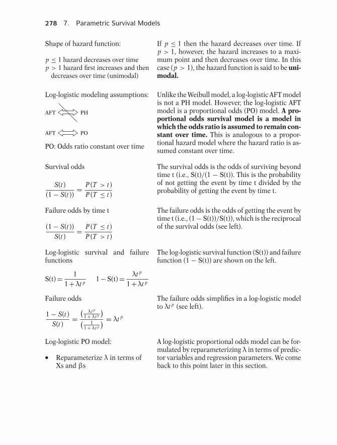
278 7. Parametric Survival Models
Shape of hazard function:
p ≤ 1 hazard decreases over timep > 1 hazard first increases and then
decreases over time (unimodal)
If p ≤ 1 then the hazard decreases over time. Ifp > 1, however, the hazard increases to a maxi-mum point and then decreases over time. In thiscase (p > 1), the hazard function is said to be uni-modal.
Log-logistic modeling assumptions:
AFT
AFT
PH
PO
PO: Odds ratio constant over time
Unlike the Weibull model, a log-logistic AFT modelis not a PH model. However, the log-logistic AFTmodel is a proportional odds (PO) model. A pro-portional odds survival model is a model inwhich the odds ratio is assumed to remain con-stant over time. This is analogous to a propor-tional hazard model where the hazard ratio is as-sumed constant over time.
Survival odds
S(t)(1 − S(t))
= P (T > t)P (T ≤ t)
The survival odds is the odds of surviving beyondtime t (i.e., S(t)/(1 − S(t)). This is the probabilityof not getting the event by time t divided by theprobability of getting the event by time t.
Failure odds by time t
(1 − S(t))S(t)
= P (T ≤ t)P (T > t)
The failure odds is the odds of getting the event bytime t (i.e., (1 − S(t))/S(t)), which is the reciprocalof the survival odds (see left).
Log-logistic survival and failurefunctions
S(t) = 11 +λt p
1 − S(t) = λt p
1 +λt p
The log-logistic survival function (S(t)) and failurefunction (1 − S(t)) are shown on the left.
Failure odds
1 − S(t)S(t)
=(
λt p
1 + λt p
)( 11 + λt p
) = λt p
The failure odds simplifies in a log-logistic modelto λt p (see left).
Log-logistic PO model:
� Reparameterize λ in terms ofXs and βs
A log-logistic proportional odds model can be for-mulated by reparameterizing λ in terms of predic-tor variables and regression parameters. We comeback to this point later in this section.
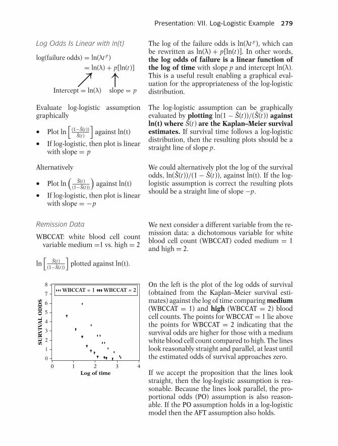
Presentation: VII. Log-Logistic Example 279
Log Odds Is Linear with ln(t)
log(failure odds) = ln(λt p)
= ln(λ) + p[ln(t)]↗ ↑Intercept = ln(λ) slope = p
The log of the failure odds is ln(λt p), which canbe rewritten as ln(λ) + p[ln(t)]. In other words,the log odds of failure is a linear function ofthe log of time with slope p and intercept ln(λ).This is a useful result enabling a graphical eval-uation for the appropriateness of the log-logisticdistribution.
Evaluate log-logistic assumptiongraphically
� Plot ln[
(1−S(t))S(t)
]against ln(t)
� If log-logistic, then plot is linearwith slope = p
The log-logistic assumption can be graphicallyevaluated by plotting ln(1 − S(t))/(S(t)) againstln(t) where S(t) are the Kaplan–Meier survivalestimates. If survival time follows a log-logisticdistribution, then the resulting plots should be astraight line of slope p.
Alternatively
� Plot ln(
S(t)(1−S(t))
)against ln(t)
� If log-logistic, then plot is linearwith slope = −p
We could alternatively plot the log of the survivalodds, ln(S(t))/(1 − S(t)), against ln(t). If the log-logistic assumption is correct the resulting plotsshould be a straight line of slope −p.
Remission Data
WBCCAT: white blood cell countvariable medium =1 vs. high = 2
We next consider a different variable from the re-mission data: a dichotomous variable for whiteblood cell count (WBCCAT) coded medium = 1and high = 2.
ln[
S(t)(1−S(t))
]plotted against ln(t).
0 1 2 3 4
0
1
2
3
4
5
7
6
8WBCCAT = 1 WBCCAT = 2
Log of time
SU
RV
IVA
L O
DD
S
On the left is the plot of the log odds of survival(obtained from the Kaplan–Meier survival esti-mates) against the log of time comparing medium(WBCCAT = 1) and high (WBCCAT = 2) bloodcell counts. The points for WBCCAT = 1 lie abovethe points for WBCCAT = 2 indicating that thesurvival odds are higher for those with a mediumwhite blood cell count compared to high. The lineslook reasonably straight and parallel, at least untilthe estimated odds of survival approaches zero.
If we accept the proposition that the lines lookstraight, then the log-logistic assumption is rea-sonable. Because the lines look parallel, the pro-portional odds (PO) assumption is also reason-able. If the PO assumption holds in a log-logisticmodel then the AFT assumption also holds.

280 7. Parametric Survival Models
Straight lines Log-logistic
Parallel plots PO
Log-logistic and PO AFT
The key points from above are:
a. straight lines support the log-logisticassumption,
b. parallel curves support the POassumption, and
c. If the log-logistic and PO assumptionshold, then the AFT assumption alsoholds.
Log-logistic and Weibull graphicalapproach analogous
� Check PH for Weibull� Check PO for log-logistic
The graphical evaluation for the log-logistic as-sumption is analogous to the graphical analysis ofthe Weibull assumption presented in the last sec-tion, except here the PO assumption rather thanthe PH assumption is evaluated by checking forparallel lines.
AFT log-logistic model
S(t) = 11 + λt p
= 1
1 + (λ1/pt)p
solve for t to obtain
t =[
1S(t)
− 1]1/p
× 1
λ1/p
let1
λ1/p= exp(α0 + α1WBCCAT)
t =[
1S(t)
− 1]1/p
× exp(α0 + α1WBCCAT)↗Scaling of t
Next we consider an AFT log-logistic model withwhite blood cell count as the only predictor com-paring WBCCAT = 2 (high count) and WBCCAT= 1 (medium count).
We develop the AFT parameterization bysolving for t in terms of a fixed S(t). Startingwith the expression for S(t), taking reciprocals,subtracting 1, raising to the power 1/p, and thenmultiplying by the reciprocal of λ1/p, yields theexpression for t shown on the left. By reparameter-izing 1/λ1/p = exp(α0 + α1WBCCAT), we allowthe predictor variable WBCCAT to be used for themultiplicative scaling of time to any fixed value ofS(t) (see left).
Let S(t) = q
t = [q−1 − 1]1/p
× exp(α0 + α1WBCCAT)
Median survival time (q = 0.5):
tm = [2 − 1]1/p
× exp(α0 + α1WBCCAT)
The expression for t is restated on the left in termsof any fixed probability S(t) = q. For example, tofind an expression for the median survival time tm,substitute q = 0.5 (see left).
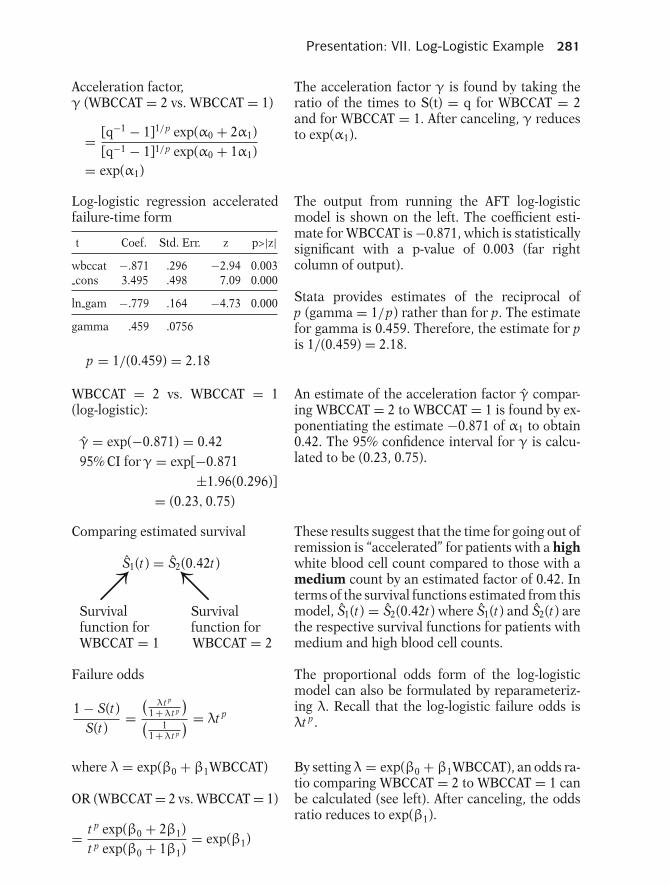
Presentation: VII. Log-Logistic Example 281
Acceleration factor,γ (WBCCAT = 2 vs. WBCCAT = 1)
= [q−1 − 1]1/p exp(α0 + 2α1)[q−1 − 1]1/p exp(α0 + 1α1)
= exp(α1)
The acceleration factor γ is found by taking theratio of the times to S(t) = q for WBCCAT = 2and for WBCCAT = 1. After canceling, γ reducesto exp(α1).
Log-logistic regression acceleratedfailure-time form
t Coef. Std. Err. z p>|z|wbccat −.871 .296 −2.94 0.003cons 3.495 .498 7.09 0.000
ln gam −.779 .164 −4.73 0.000
gamma .459 .0756
p = 1/(0.459) = 2.18
The output from running the AFT log-logisticmodel is shown on the left. The coefficient esti-mate for WBCCAT is −0.871, which is statisticallysignificant with a p-value of 0.003 (far rightcolumn of output).
Stata provides estimates of the reciprocal ofp (gamma = 1/p) rather than for p. The estimatefor gamma is 0.459. Therefore, the estimate for pis 1/(0.459) = 2.18.
WBCCAT = 2 vs. WBCCAT = 1(log-logistic):
γ = exp(−0.871) = 0.4295% CI for γ = exp[−0.871
±1.96(0.296)]= (0.23, 0.75)
An estimate of the acceleration factor γ compar-ing WBCCAT = 2 to WBCCAT = 1 is found by ex-ponentiating the estimate −0.871 of α1 to obtain0.42. The 95% confidence interval for γ is calcu-lated to be (0.23, 0.75).
Comparing estimated survival
S1(t) = S2(0.42t)↗ ↖Survival Survivalfunction for function forWBCCAT = 1 WBCCAT = 2
These results suggest that the time for going out ofremission is “accelerated” for patients with a highwhite blood cell count compared to those with amedium count by an estimated factor of 0.42. Interms of the survival functions estimated from thismodel, S1(t) = S2(0.42t) where S1(t) and S2(t) arethe respective survival functions for patients withmedium and high blood cell counts.
Failure odds
1 − S(t)S(t)
=(
λt p
1 + λt p
)( 11 + λt p
) = λt p
The proportional odds form of the log-logisticmodel can also be formulated by reparameteriz-ing λ. Recall that the log-logistic failure odds isλt p.
where λ = exp(β0 + β1WBCCAT)
OR (WBCCAT = 2 vs. WBCCAT = 1)
= t p exp(β0 + 2β1)t p exp(β0 + 1β1)
= exp(β1)
By setting λ = exp(β0 + β1WBCCAT), an odds ra-tio comparing WBCCAT = 2 to WBCCAT = 1 canbe calculated (see left). After canceling, the oddsratio reduces to exp(β1).
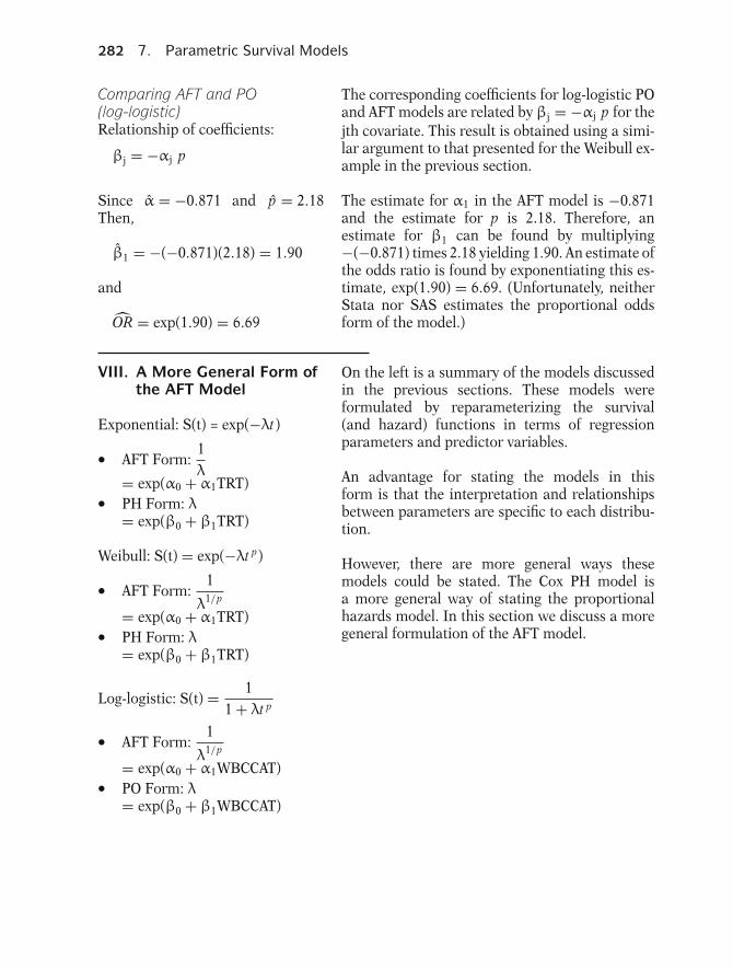
282 7. Parametric Survival Models
Comparing AFT and PO(log-logistic)Relationship of coefficients:
βj = −αj p
The corresponding coefficients for log-logistic POand AFT models are related by βj = −αj p for thejth covariate. This result is obtained using a simi-lar argument to that presented for the Weibull ex-ample in the previous section.
Since α = −0.871 and p = 2.18Then,
β1 = −(−0.871)(2.18) = 1.90
and
OR = exp(1.90) = 6.69
The estimate for α1 in the AFT model is −0.871and the estimate for p is 2.18. Therefore, anestimate for β1 can be found by multiplying−(−0.871) times 2.18 yielding 1.90. An estimate ofthe odds ratio is found by exponentiating this es-timate, exp(1.90) = 6.69. (Unfortunately, neitherStata nor SAS estimates the proportional oddsform of the model.)
VIII. A More General Form ofthe AFT Model
Exponential: S(t) = exp(−λt)
� AFT Form:1λ= exp(α0 + α1TRT)� PH Form: λ
= exp(β0 + β1TRT)
Weibull: S(t) = exp(−λt p)
� AFT Form:1
λ1/p
= exp(α0 + α1TRT)� PH Form: λ= exp(β0 + β1TRT)
Log-logistic: S(t) = 11 + λt p
� AFT Form:1
λ1/p
= exp(α0 + α1WBCCAT)� PO Form: λ= exp(β0 + β1WBCCAT)
On the left is a summary of the models discussedin the previous sections. These models wereformulated by reparameterizing the survival(and hazard) functions in terms of regressionparameters and predictor variables.
An advantage for stating the models in thisform is that the interpretation and relationshipsbetween parameters are specific to each distribu-tion.
However, there are more general ways thesemodels could be stated. The Cox PH model isa more general way of stating the proportionalhazards model. In this section we discuss a moregeneral formulation of the AFT model.
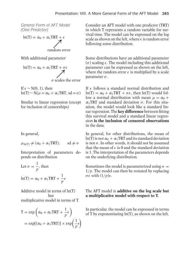
Presentation: VIII. A More General Form of the AFT Model 283
General Form of AFT Model(One Predictor)
ln(T) = α0 + α1TRT + ε↗random error
Consider an AFT model with one predictor (TRT)in which T represents a random variable for sur-vival time. The model can be expressed on the logscale as shown on the left, where ε is random errorfollowing some distribution.
With additional parameter
ln(T) = α0 + α1TRT + σε↗σ scales the error
Some distributions have an additional parameter(σ ) scaling ε. The model including this additionalparameter can be expressed as shown on the left,where the random error ε is multiplied by a scaleparameter σ .
If ε ∼ N(0, 1), thenln(T) ∼ N(µ =α0 + α1TRT, sd = σ )
Similar to linear regression (exceptfor inclusion of censorships)
If ε follows a standard normal distribution andln(T) = α0 + α1TRT + σε, then ln(T) would fol-low a normal distribution with mean µ = α0 +α1TRT and standard deviation σ . For this situ-ation, the model would look like a standard lin-ear regression. The key difference between fittingthis survival model and a standard linear regres-sion is the inclusion of censored observationsin the data.
In general,
µln(T) �= (α0 + α1TRT), sd �= σ
Interpretation of parameters de-pends on distribution
In general, for other distributions, the mean ofln(T) is not α0 + α1TRT and its standard deviationis not σ . In other words, it should not be assumedthat the mean of ε is 0 and the standard deviationis 1. The interpretation of the parameters dependson the underlying distribution.
Let σ = 1p
, then
ln(T) = α0 + α1TRT + 1pε
Sometimes the model is parameterized using σ =1/p. The model can then be restated by replacingσε with (1/p)ε.
Additive model in terms of ln(T)but
multiplicative model in terms of T
The AFT model is additive on the log scale buta multiplicative model with respect to T.
T = exp(α0 + α1TRT + 1
pε
)= exp[(α0 + α1TRT)] × exp
(1pε
)In particular, the model can be expressed in termsof T by exponentiating ln(T), as shown on the left.

284 7. Parametric Survival Models
Collapse α0 into baseline term
T0 = exp(α0) exp(
1pε
)so that T = exp(α1TRT) × T0where T0 is a random variable forTRT = 0
The model may also be expressed by collapsing theintercept into a baseline random term T0 (see left).In this setting T0 is a random variable representingthe survival time of the placebo group (TRT = 0).
AFT model may be expressed interms of T or ln(T)
Comparing Distributions: T andln(T)
T ln(T)
Exponential Extreme minimumvalue
Weibull Extreme minimumvalue
Log-logistic LogisticLognormal Normal
In summary, an AFT model may be expressed byreparameterizing a specific distribution, or maybe more generally expressed either in terms of arandom variable T (for survival time), or ln(T).If T follows a Weibull distribution then ln(T) fol-lows a distribution called the extreme minimumvalue distribution (see table on left). Similarly, ifT follows a log-logistic or lognormal distributionthen ln(T) follows a logistic or normal distribu-tion, respectively. The logistic and normal distri-butions are similarly shaped, and are both sym-metric about their mean.
IX. Other Parametric Models In the previous sections we presented examples ofthe exponential, Weibull, and log-logistic models.In this section we briefly discuss some other para-metric survival models.
Generalized Gamma Model
� Supported by SAS and Stata� S(t), h(t) expressed in termsof integrals� Contains three parameters� Weibull, lognormal are specialcases
The generalized gamma model is a parametricsurvival model that is supported by both SAS andStata software. The hazard and survival functionfor this model is complicated and can only beexpressed in terms of integrals. The generalizedgamma distribution has three parameters allow-ing for great flexibility in its shape. The Weibulland lognormal distributions are special cases ofthe generalized gamma distribution (see PracticeExercises 12 to 14).
Lognormal Model
Similar to log-logisticDifference:
Log-logistic: AFT and POLognormal: AFT but not PO
The lognormal model also has a relatively com-plicated hazard and survival function that can onlybe expressed in terms of integrals. The shape ofthe lognormal distribution is very similar to thelog-logistic distribution and yields similar modelresults. A difference is that although the lognor-mal model accommodates an accelerated failuretime model, it is not a proportional odds model.
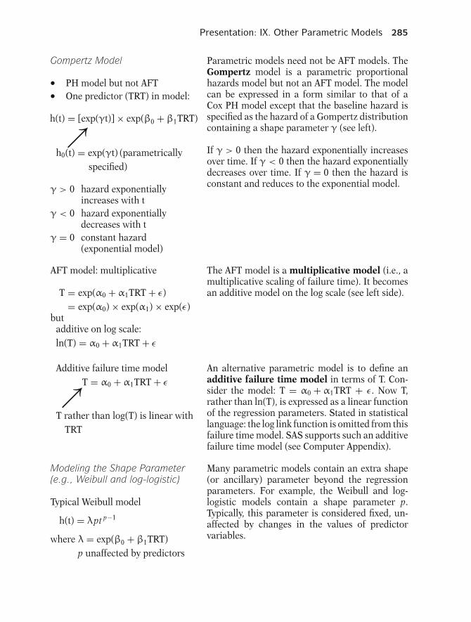
Presentation: IX. Other Parametric Models 285
Gompertz Model
� PH model but not AFT� One predictor (TRT) in model:
h(t) = [exp(γt)] × exp(β0 + β1TRT)
↗h0(t) = exp(γt) (parametrically
specified)
γ > 0 hazard exponentiallyincreases with t
γ < 0 hazard exponentiallydecreases with t
γ = 0 constant hazard(exponential model)
Parametric models need not be AFT models. TheGompertz model is a parametric proportionalhazards model but not an AFT model. The modelcan be expressed in a form similar to that of aCox PH model except that the baseline hazard isspecified as the hazard of a Gompertz distributioncontaining a shape parameter γ (see left).
If γ > 0 then the hazard exponentially increasesover time. If γ < 0 then the hazard exponentiallydecreases over time. If γ = 0 then the hazard isconstant and reduces to the exponential model.
AFT model: multiplicative
T = exp(α0 + α1TRT + ε)= exp(α0) × exp(α1) × exp(ε)
butadditive on log scale:ln(T) = α0 + α1TRT + ε
Additive failure time modelT = α0 + α1TRT + ε↗
T rather than log(T) is linear withTRT
The AFT model is a multiplicative model (i.e., amultiplicative scaling of failure time). It becomesan additive model on the log scale (see left side).
An alternative parametric model is to define anadditive failure time model in terms of T. Con-sider the model: T = α0 + α1TRT + ε. Now T,rather than ln(T), is expressed as a linear functionof the regression parameters. Stated in statisticallanguage: the log link function is omitted from thisfailure time model. SAS supports such an additivefailure time model (see Computer Appendix).
Modeling the Shape Parameter(e.g., Weibull and log-logistic)
Typical Weibull model
h(t) = λpt p−1
where λ = exp(β0 + β1TRT)p unaffected by predictors
Many parametric models contain an extra shape(or ancillary) parameter beyond the regressionparameters. For example, the Weibull and log-logistic models contain a shape parameter p.Typically, this parameter is considered fixed, un-affected by changes in the values of predictorvariables.

286 7. Parametric Survival Models
Alternative Weibull modelmodels the ancillary parameter p
h(t) = λpt p−1
where λ = exp(β0 + β1TRT)p = exp(δ0 + δ1TRT)
Not a PH or AFT model if δ1 �= 0but still a Weibull model
An alternative approach is to model the shape pa-rameter in terms of predictor variables and regres-sion coefficients. In the Weibull model shown onthe left, both λ and p are modeled as functions oftreatment status (TRT). If δ1 is not equal to zero,then the value of p differs by TRT. For that sit-uation, the PH (and thus the AFT) assumption isviolated because t p−1 will not cancel in the hazardratio for TRT (see Practice Exercises 15 to 17).
Choosing appropriate model
� Evaluate graphically◦ Exponential◦ Weibull◦ Log-logistic� Akaike’s information criterion◦ Compares model fit◦ Uses −2 log likelihood
Choosing the most appropriate parametric modelcan be difficult. We have provided graphical ap-proaches for evaluating the appropriateness ofthe exponential, Weibull, and log-logistic models.Akaike’s information criterion (AIC) providesan approach for comparing the fit of models withdifferent underlying distributions, making use ofthe −2 log likelihood statistic (described in Prac-tice Exercises 11 and 14).
X. The Parametric Likelihood
� Function of observed data andunknown parameters� Based on outcome distributionf(t)� Censoring complicates survivaldata◦ Right-censored◦ Left-censored◦ Interval-censored
The likelihood for any parametric model is a func-tion of the observed data and the model’s un-known parameters. The form of the likelihoodis based on the probability density function f(t)of the outcome variable. A complication of sur-vival data is the possible inclusion of censoredobservations (i.e., observations in which the ex-act time of the outcome is unobserved). We con-sider three types of censored observations: right-censored, left-censored, and interval-censored.
Examples of Censored Subjects
Right-censored:10
10
108
Left-censored: __________________ time
Interval-censored: ______________ time
x
x
x
time
Right-censored. Suppose a subject is lost tofollow-up after 10 years of observation. The timeof event is not observed because it happened af-ter the 10th year. This subject is right-censored at10 years because the event happened to the rightof 10 on the time line (i.e., t > 10).
Left-censored. Suppose a subject had an event be-fore the 10th year but the exact time of the event isunknown. This subject is left-censored at 10 years(i.e., t < 10).
Interval-censored. Suppose a subject had anevent between the 8th and 10th year (exact timeunknown). This subject is interval-censored (i.e.,8 < t < 10).

Presentation: X. The Parametric Likelihood 287
Formulating the Likelihood
Barry, Gary, Larry, . . . , OutcomeDistribution f (t)
Event LikelihoodSubject Time Contribution
Barry t = 2 f (2)
Gary t > 8(right-censored)
∞∫8
f (t)dt
Harry t = 6 f (6)
Carrie t < 2(left-censored)
2∫0
f (t)dt
Larry 4 < t < 8(interval-censored)
8∫4
f (t)dt
The table on the left illustrates how the likelihoodis formulated for data on five subjects. We assumea probability density function f(t) for the outcome.Barry gets the event at time t = 2. His contribu-tion to the likelihood is f(2). Gary is right-censoredat t = 8. The probability that Gary gets the eventafter t = 8 is found by integrating f(t) from 8 to in-finity. This is Gary’s contribution to the likelihood.Harry gets the event at time t = 6. His contribu-tion to the likelihood is f(6). Carrie is left-censoredat t = 2. Her contribution to the likelihood is ob-tained by integrating f(t) from zero to 2. Finally,Larry is interval-censored between t = 4 and t =8. His contribution to the likelihood is found byintegrating f(t) from 4 to 8.
Likelihood (L)
Product of individual contributions
L = f (2) ×∞∫
8
f (t)dt × f (6)
×∫ 2
0f (t)dt ×
8∫4
f (t)dt
(Barry × Gary × Harry× Carrie× Larry)
The full likelihood (L) is found by taking the prod-uct of each subject’s independent contribution tothe likelihood. The likelihood for this example isshown on the left.
Assumptions for formulating L
� No competing risks◦ Competing event does not
prohibit event of interest◦ Death of all causes is
classic example of nocompeting risk
The formulation of this likelihood uses the as-sumption of no competing risks. In other words,we assume that no competing event will prohibitany subject from eventually getting the event ofinterest (see Chapter 9). Death from all causes isthe classic example of an outcome that in realityhas no competing risk. For other outcomes, the nocompeting risk assumption is more of a theoreti-cal construct.
� Subjects independent◦ Allows L to be formulated as
product of subjects’contributions
Another assumption is that individual contri-butions to the likelihood are independent. Thisassumption allows the full likelihood to be formu-lated as the product of each individual’s contribu-tion.

288 7. Parametric Survival Models
� Follow-up time continuous◦ No gaps in follow-up
A third assumption is that each subject’s follow-uptime is continuous without gaps (i.e., once sub-jects are out of the study, they do not return). Ifgaps are allowed, the likelihood can be modifiedto accommodate such a scenario.
Revisit example with Barry, Gary,Larry, . . .f(t) is WeibullSMOKE is only predictor
1 = Smoker0 = Nonsmoker
Weibull: h(t) = λpt p−1,S(t) = exp(−λt p)
f (t) = h(t)S(t)f (t) = λpt p−1 exp(−λt p)
where λ = exp(β0 + β1SMOKE)(PH form of the model)
In the last example, we did not specify the prob-ability density f(t), nor did we specify any co-variates. We revisit this example, assuming f(t) isWeibull with one predictor SMOKE in the model(coded 1 for smokers and 0 for nonsmokers).
The Weibull hazard and survival functions areshown on the left. The probability density func-tion f(t) is the product of the hazard and survivalfunctions. The parameterization will use the pro-portional hazards (PH) form of the Weibull model:λ = β0 + β1SMOKE.
Data Layout for Right-, Left-, andInterval-Censoring Using SAS
ID LOWER UPPER SMOKE
Barry 2 2 1Gary 8 — 0Harry 6 6 0Carrie — 2 0Larry 4 8 1
Right-censored: UPPER missingLeft-censored: LOWER missingInterval-censored: LOWER <
UPPERNot censored: LOWER = UPPER
On the left is the data layout for running paramet-ric models containing right-, left-, and interval-censored data in a form suitable for using theSAS procedure PROC LIFETEST (version 8.2).There are two time variables LOWER and UPPER.Barry got the event at t = 2, so both LOWER andUPPER get the value 2. Gary was right-censoredat 8 (t >8) so LOWER gets the value 8 and UP-PER is set to missing. Carrie is left-censored at 2(t < 2) so LOWER is set to missing and UPPERgets the value 2. Larry was interval-censored withLOWER = 4 and UPPER = 8. Barry and Larryare smokers whereas Gary, Harry, and Carrie arenonsmokers.
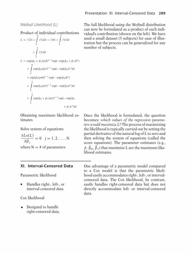
Presentation: XI. Interval-Censored Data 289
Weibull Likelihood (L)
Product of individual contributions
L = f (2) ×∞∫
8
f (t)dt × f (6) ×2∫
0
f (t)dt
×8∫
4
f (t)dt
L = exp(β0 + β1)p(2)p−1exp(−exp(β0 + β1)2p)
×∞∫
8
exp(β0)p(t)p−1 exp(− exp(β0)t p)dt
× exp(β0)p(6)p−1 exp(− exp(β0)6p)
×2∫
0
exp(β0)p(t)p−1 exp(− exp(β0)t p)dt
×8∫
4
exp(β0 + β1)p(t)p−1 exp(− exp(β0
+ β1)t p)dt
Obtaining maximum likelihood es-timates
Solve system of equations:
∂Ln(L)∂β j
= 0 j = 1, 2, . . . , N
where N = # of parameters
The full likelihood using the Weibull distributioncan now be formulated as a product of each indi-vidual’s contribution (shown on the left). We haveused a small dataset (5 subjects) for ease of illus-tration but the process can be generalized for anynumber of subjects.
Once the likelihood is formulated, the questionbecomes: which values of the regression parame-ters would maximize L? The process of maximizingthe likelihood is typically carried out by setting thepartial derivative of the natural log of L to zero andthen solving the system of equations (called thescore equations). The parameter estimates (e.g.,p, β0, β1) that maximize L are the maximum like-lihood estimates.
XI. Interval-Censored Data
Parametric likelihood
� Handles right-, left-, orinterval-censored data
Cox likelihood
• Designed to handleright-censored data.
One advantage of a parametric model comparedto a Cox model is that the parametric likeli-hood easily accommodates right-, left-, or interval-censored data. The Cox likelihood, by contrast,easily handles right-censored data but does notdirectly accommodate left- or interval-censoreddata.
290 7. Parametric Survival Models
Interval-censored study design
� Check for nonsymptomaticoutcome once a year� If outcome newly detected,exact time occurred duringprevious year� Left-censoring special case ofinterval-censoring◦ Zero the lower boundary of
the interval
Sometimes the design of a study is such that allthe data are interval-censored. For example, con-sider a study in which healthcare workers exam-ine subjects once a year, checking for a nonsymp-tomatic outcome. If an event was first detectedin the beginning of the third year, then the ex-act time of the outcome occurred sometime be-tween the second and third years. In this frame-work left-censoring can be considered a specialcase of interval-censoring with zero as the lowerboundary of the interval.
Parametric model can be fitted
� f(t) specified� Contribution to likelihood foreach subject◦ Integrate f(t) over event
interval
A parametric model can easily be fitted using themethods described in the previous section. Once adistribution for the outcome, f(t), is specified, eachsubject’s contribution to the likelihood is obtainedby integrating f(t) over the interval in which he orshe had the event.
Binary regression
� Alternative approachfor interval-censored data� Outcome coded◦ 0 if subject survives interval◦ 1 if subject gets event during
interval� Useful approach if◦ Ample number of events in
each interval◦ Prefer not to specify f(t)
A binary regression (e.g., logistic regression) isan alternative approach that may be consideredif all the data are interval-censored. With thismethod the outcome variable can be coded zeroif the subject survives the interval and coded oneif the subject gets the event during the interval.This approach is particularly useful if there are anample number of events in each interval and theanalyst prefers not to specify a distribution f(t) forcontinuous survival time.
Information on Three Subjects
Subject 1: Gets event in first intervalSubject 2: Survives first interval
Survives second intervalGets event in thirdinterval
Subject 3: Survives first intervalGets event in secondinterval
For illustration, consider a small dataset contain-ing three subjects. Subject 1 gets the event in thefirst interval of follow-up, subject 2 gets the eventin the third interval, and subject 3 gets the eventin the second interval of follow-up.

Presentation: XI. Interval-Censored Data 291
Data Layout for Binary Regression
SUBJECT EVENT D1 D2 D3 TRT
1 1 1 0 0 12 0 1 0 0 02 0 0 1 0 02 1 0 0 1 03 0 1 0 0 13 1 0 1 0 1
EVENT: dichotomous outcomecoded 1 if event, 0 for no eventduring the interval
D1, D2, D3: dummy variables forintervals 1, 2, and 3 coded 1 if in thecorresponding interval, 0 otherwise
TRT: Treatment coded 1 for newtreatment, 0 for placebo
The data layout is shown on the left. Eachobservation represents one interval of follow-uptime allowing multiple observations per subject.EVENT is the dichotomous outcome variable.Subject 1 had the event in the first interval(EVENT = 1) and thus has one observation.Subject 2 has three observations because shesurvived the first two intervals (EVENT = 0) butgot the event in the third interval. D1 is a dummyvariable coded 1 if the observation representsthe first interval and 0 otherwise. Similarly, D2 iscoded 1 for the second interval and D3 is coded 1for the third interval.
TRT is the predictor of interest, coded 1 forthe new treatment and 0 for the placebo. TRTcould be coded as a time-independent or time-dependent variable. In this example, TRT istime-independent because TRT does not changevalues over different intervals corresponding tothe same subject.
Logistic Model
Logit P(Y = 1) = β1D1 + β2D2
+β3D3 + β4TRT
where P(Y = 1) is the probabilityof event for a given interval condi-tioned on survival of previous inter-vals
A logistic model (shown at left) containing thethree dummy variables and TRT can be formu-lated with the data in this form.
Interpretation of Parameters
β1: Log odds of event in 1st intervalamong TRT = 0
β2: Log odds of event in 2nd inter-val given survival of 1st intervalamong TRT = 0
β3: Log odds of event in 3rd intervalgiven survival of first two inter-vals among TRT = 0
β4: Log odds ratio for TRT
Care must be taken with the interpretation of theparameters: β1 is the log odds of the event occur-ring in the first interval among the placebo group;β2 is the log odds of the event occurring in the sec-ond interval conditioned on survival of the first in-terval among the placebo group; β3 is the log oddsof the event occurring in the third interval condi-tioned on survival of the first and second intervalsamong the placebo group; and β4 is the log oddsratio for TRT.
292 7. Parametric Survival Models
D1, D2, D3 play similar role as inter-cept
� Baseline measure whencovariates are zero� 3 parameters rather than 1intercept◦ Baseline measure may differ
for each interval
The dummy variables play a similar role to thatof the intercept in a conventional regression, pro-viding a baseline outcome measure for the case inwhich all predictors are zero (e.g., TRT = 0). Ingeneral, the baseline measure may differ for eachinterval, which is the reason that the model con-tains 3 dummy variables rather than 1 intercept.
Odds Ratio (TRT = 1 vs. TRT = 0)= exp(β4)
Model uses PO assumption
� OR constant over time� PO assumption can be tested◦ Include interaction terms
with TRT and dummyvariables
◦ Significant interactionsuggests PO violation
◦ Need ample data topractically carry out test
The odds ratio comparing TRT = 1 to TRT = 0 isobtained by exponentiating β4. This model usesthe proportional odds (PO) assumption in thatthe odds ratio is assumed constant over time (orat least constant at the end of each interval). Thisassumption can be tested by including interaction(product) terms with TRT and two of the dummyvariables in the model. A statistically significantproduct term would suggest a violation of the POassumption. However, if there are sparse data cor-responding to particular intervals, it will not bepractical to carry out such a test on those inter-vals.
Alternative Binary Model
log(− log(1 − P(Y = 1)))= β1D1 + β2D2 + β3D3 + β4TRT
where 1 − P(Y = 1) is the probabil-ity of surviving a given interval con-ditioned on survival of previous in-tervals
Logistic regression is not the only type of binaryregression that may be considered for interval-censored data. An alternative binary model(shown on the left) uses the complementary log–log link function rather than the logit link func-tion that is used for the more familiar logisticregression.
Complementary log–log link� Log–log survival modeled aslinear function of regressionparameters
Logit link� Log odds of failure modeledas linear function of regressionparameters
A model using a complementary log–log link func-tion expresses the log negative log survival prob-ability as a linear function of regression param-eters. By contrast, a model using a logit linkfunction expresses the log odds of failure (i.e., get-ting the event) as a linear function of regressionparameters.

Presentation: XI. Interval-Censored Data 293
Complementary log–log model isPH model
� HR (TRT = 1 vs. TRT = 0) =exp(β4)� HR constant over time
The complementary log–log binary model is aproportional hazards model. The hazard ratiocomparing TRT = 1 to TRT = 0 is obtained byexponentiating β4.
Log–log survival curves:parallel additive effects
PH
Complementary log–log link:additive effects on log–log scale
PH
Recall we can use log–log survival curves to eval-uate the PH assumption for a Cox model. If theeffects are additive (e.g., parallel for TRT = 1 andTRT = 0) then the PH assumption is assumed tohold. The underlying idea is similar for the com-plementary log–log link function in that additiveeffects are assumed on the log–log scale (e.g., com-paring TRT = 1 to TRT = 0).
In theory� Survival time is continuous
In practice� Survival time measured inintervals◦ If event occured in month 7
then event occurred in aninterval of time
In theory, the time-to-event variable in survivalanalyses is thought of as a continuous variable.In practice, however, the time variable is typicallyan interval of time. For example, if time is mea-sured in months and an event occurs in month 7then the event is recorded as having occurred in aspecific interval lasting a month.
Discrete survival analysis
� Discrete time� For example, number ofmenstrual cycles to pregnancyrather than time to pregnancy◦ Fraction of cycle does not
make sense
Discrete survival analysis is a survival analysisin which the outcome variable is discrete, both intheory and in practice. For example, consider astudy in which women who stop using oral con-traception are followed until pregnancy. The out-come is defined as the number of menstrual cy-cles until pregnancy. The number of cycles ratherthan the time to pregnancy is used because thecycle length varies among women and a womanovulates only once per menstrual cycle (i.e., oneopportunity per cycle to become pregnant). Thenumber of cycles is a discrete outcome. A fractionof a cycle does not make sense.

294 7. Parametric Survival Models
Analyzing discrete survival data
� Can use binary regression� Analogous to interval-censoreddata◦ Discrete outcome—subjects
survive discrete units of time◦ Interval outcomes—
subjects survive intervalsof time
Binary regression, as described in this section,can be applied for discrete survival outcomes ina similar manner to that described for interval-censored outcomes. With this method, subjectscan be conceptualized as surviving discrete unitsof time analogously as subjects surviving continu-ous intervals of time.
XII. Frailty Models
Frailty
� Random component� Accounts for extra variabilityfrom unobserved factors
In this section we consider the inclusion of frailtyto a survival model. Frailty is a random compo-nent designed to account for variability due tounobserved individual-level factors that is other-wise unaccounted for by the other predictors inthe model.
Conceptualize S(t) two ways:
� For an individual� Averaging over a theoreticallarge population
Consider a survival model with a continuous agevariable and dichotomous smoking status variableas the only predictors. Under this model the sur-vival function for a 33-year-old smoker might beconceptualized in different ways. One way is asthe survival function for an individual 33-year-oldsmoker. The second way is as some kind of averag-ing over a theoretical large population of 33-year-old smokers.
With Frailty Component
Jake and Blake1. May have different S(t) due to
unobserved factors2. Extra source of variability in
outcome (e.g., more variationthan expected under Weibull)
Without Frailty Component
Jake and Blake1. Have same S(t)2. May have different event times
because event time is random,following some distribution (e.g.,Weibull)
Now suppose a “frailty” component is included inthe model. Under this model, we can conceptu-alize survival functions specific to each individ-ual. If Jake and Blake are both 33-year-old smok-ers, not only might their observed failure timesbe different, but under this model their individ-ual survival functions could also be different.Jake may be more “frail” than Blake due to un-observed factors accounting for individual leveldifferences in his hazard and survival functions.These unobserved factors may contribute an ex-tra layer of heterogeneity, leading to greater vari-ability in survival times than might be expectedunder the model (e.g., Weibull) without the frailtycomponent.
Presentation: XII. Frailty Models 295
The frailty component α (α> 0)
� Unobserved multiplicativeeffect on hazard� Follows distribution g(α) withµ = 1� Var(g(α)) = θ , parameter to beestimated
Hazard and survival conditioned onfrailty
h(t|α) =αh(t)S(t|α) = S(t)α
The frailty α is an unobserved multiplicative ef-fect on the hazard function assumed to followsome distribution g(α) with α > 0 and the meanof g(α) equal to 1. The variance of g(α) is a param-eter θ (theta) that is typically estimated from thedata.
An individual’s hazard function conditional on thefrailty can be expressed as α multiplied by h(t).Using the relationship between the survival andhazard functions, the corresponding conditionalsurvival function can be expressed as S(t) raisedto the α power.
α > 1� Increased hazard: αh(t) > h(t)� Decreased survival: S(t)α < S(t)
α < 1� Decreased hazard: αh(t) < h(t)� Increases survival: S(t)α > S(t)
α = 1 (average frailty): αh(t) = h(t)
Individuals with α > 1 have an increased hazardand decreased probability of survival compared tothose of average frailty (α = 1). Similarly, individ-uals with α < 1 have a decreased hazard and in-creased probability of survival compared to thoseof average frailty.
Survival functions(with frailty models)
1. Conditional, S(t|α), individuallevel
2. Unconditional, S∪(t), populationlevel
Unconditional survival functionS∪(t)
S∪(t) =∞∫
0
S(t |α)g (α)dα
hU (t) = −d[SU (t)]/dtSU (t)
With frailty models, we distinguish the individ-ual level or conditional survival function S(t|α)discussed above, from the population level or un-conditional survival function S∪(t), which repre-sents a population average. Once the frailty distri-bution g(α) is chosen, the unconditional survivalfunction is found by integrating over the condi-tional survival function S(t|α) times g(α), withrespect to α. The corresponding unconditionalhazard h∪(t) can then be found using the relation-ship between the survival and hazard functions(see left).
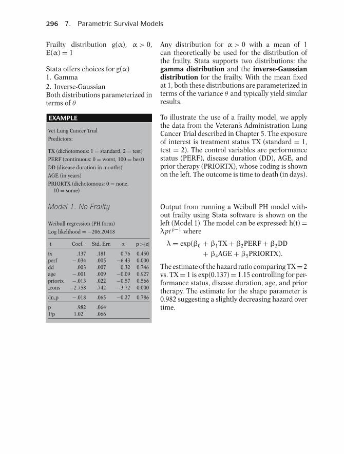
296 7. Parametric Survival Models
Frailty distribution g(α), α > 0,E(α) = 1
Stata offers choices for g(α)1. Gamma2. Inverse-GaussianBoth distributions parameterized interms of θ
Any distribution for α > 0 with a mean of 1can theoretically be used for the distribution ofthe frailty. Stata supports two distributions: thegamma distribution and the inverse-Gaussiandistribution for the frailty. With the mean fixedat 1, both these distributions are parameterized interms of the variance θ and typically yield similarresults.
EXAMPLE
Vet Lung Cancer Trial
Predictors:
TX (dichotomous: 1 = standard, 2 = test)
PERF (continuous: 0 = worst, 100 = best)
DD (disease duration in months)
AGE (in years)
PRIORTX (dichotomous: 0 = none,10 = some)
To illustrate the use of a frailty model, we applythe data from the Veteran’s Administration LungCancer Trial described in Chapter 5. The exposureof interest is treatment status TX (standard = 1,test = 2). The control variables are performancestatus (PERF), disease duration (DD), AGE, andprior therapy (PRIORTX), whose coding is shownon the left. The outcome is time to death (in days).
Model 1. No Frailty
Weibull regression (PH form)
Log likelihood = −206.20418
t Coef. Std. Err. z p >|z|tx .137 .181 0.76 0.450perf −.034 .005 −6.43 0.000dd .003 .007 0.32 0.746age −.001 .009 −0.09 0.927priortx −.013 .022 −0.57 0.566cons −2.758 .742 −3.72 0.000
/ln p −.018 .065 −0.27 0.786
p .982 .0641/p 1.02 .066
Output from running a Weibull PH model with-out frailty using Stata software is shown on theleft (Model 1). The model can be expressed: h(t) =λpt p−1 where
λ = exp(β0 + β1TX + β2PERF + β3DD+ β4AGE + β5PRIORTX).
The estimate of the hazard ratio comparing TX = 2vs. TX = 1 is exp(0.137) = 1.15 controlling for per-formance status, disease duration, age, and priortherapy. The estimate for the shape parameter is0.982 suggesting a slightly decreasing hazard overtime.

Presentation: XII. Frailty Models 297
EXAMPLE (continued)
Model 2. With Frailty
Weibull regression (PH form)Gamma frailtyLog likelihood = −200.11338
t Coef. Std. Err. z p >|z|tx .105 .291 0.36 0.719perf −.061 .012 −5.00 0.000dd −.006 .017 −0.44 0.663age −.013 .015 −0.87 0.385priortx −.006 .035 −0.18 0.859cons −2.256 1.100 −2.05 0.040
/ln p .435 .141 3.09 0.002/ln the −.150 .382 −0.39 0.695
p 1.54 .2171/p .647 .091theta .861 .329
Likelihood ratio test of theta = 0:chibar2(01) = 12.18Prob>=chibar2 = 0.000
Model 2 (output on left) is the same Weibull modelas Model 1 except that a frailty component hasbeen included. The frailty in Model 2 is assumedto follow a gamma distribution with mean 1 andvariance equal to theta (θ ). The estimate of thetais 0.861 (bottom row of output). A variance ofzero (theta = 0) would indicate that the frailtycomponent does not contribute to the model. Alikelihood ratio test for the hypothesis theta = 0is shown directly below the parameter estimatesand indicates a chi-square value of 12.18 with 1degree of freedom yielding a highly significantp-value of 0.000 (rounded to 3 decimals).
Notice how all the parameter estimatesare altered with the inclusion of the frailty.The estimate for the shape parameter is now 1.54,quite different from the estimate 0.982 obtainedfrom Model 1. The inclusion of frailty not onlyhas an impact on the parameter estimates butalso complicates their interpretation.
Comparing Model 2 with Model 1
� There is one additionalparameter to estimate inModel 2� The actual values ofindividuals’ frailty are notestimated in Model 2� The coefficients for thepredictor variables in Models 1and 2 have different estimatesand interpretation� The estimate of the shapeparameter is <1.0 for Model 1and >1.0 for Model 2
Before discussing in detail how the inclusionof frailty influences the interpretation of theparameters, we overview some of the key points(listed on the left) that differentiate Model 2(containing the frailty) and Model 1.
Model 2 contains one additional parameter,the variance of the frailty. However, the actualvalues of each subject’s frailty are not estimated.The regression coefficients and Weibull shapeparameter also differ in their interpretations forModel 2 compared to Model 1. We now elaborateon these points.

298 7. Parametric Survival Models
Model 2
Hazard for jth individual:
hj(t|αj) = αjh(t) j = 1, 2, . . . , n
where h(t) = λpt p−1
with λ = exp(β0 + β1TX+β2PERF + β3DD+β4AGE + β5PRIORTX)
and where α ∼ gamma (µ = 1,variance = θ )
For Model 2 we can express the Weibull modelwith a gamma distributed frailty in terms of theindividual level hazard for the jth subject.
If αj denotes the frailty for the jth subject,then that subject’s hazard hj(t|αj) can be ex-pressed as αj multiplied by h(t), where h(t) is theWeibull hazard function parameterized in termsof the predictor variables and their regressioncoefficients (see left).
αj not estimable� An αj associated with eachsubject� Too many parameters
The values for each αj are not estimable becausethere is a level of frailty associated with each datapoint. If we tried to estimate each subject’s frailty,then there would be more parameters to estimatethan observations in the dataset and the modelwould be overparameterized.
Rather, var[g(α)] is estimated� Gamma is 2-parameterdistribution◦ Mean set at 1.0◦ θ = Var[g(α)] is estimated
Rather, the variance of the frailty is estimated. Thegamma distribution is a two-parameter distribu-tion. Because the mean is set at 1, we need onlyestimate its variance to fully specify the frailty dis-tribution.
Interpreting coefficients in Model 2
H R = exp(β1) = 1.11
Estimates HR comparing two indi-viduals� With same α� One with TX = 2, other with
TX = 1� With same levels of otherpredictors
The estimated coefficient for TX using Model 2 is0.105. By exponentiating, we obtain exp(0.105) =1.11. This is the estimated hazard ratio for twoindividuals having the same frailty in which onetakes the test treatment and the other takes thestandard treatment controlling for the other co-variates in the model. Thus, for two individualswith the same frailty, we can use the coefficientestimates from Model 2 to estimate the ratio ofconditional hazards.

Presentation: XII. Frailty Models 299
Recall: h(t|α) = αh(t)
TX = 1: h1(t|α1) = α1h1(t)TX = 2: h2(t|α2) = α2h1(t)
Ifh2(t)h1(t)
= exp(β1)
thenα1�h1(t)α2� h2(t)
= exp(β1)
only if α1 = α2
To clarify, recall that the individual level or condi-tional hazard function can be expressed as a mul-tiplied by h(t). Suppose h1(t|α1) and h2(t|α2) arethe conditional hazard functions for individualswho use the standard and test treatments, respec-tively, at the mean levels of the other covariates. Ifthe ratio of h2(t) and h1(t) equals exp(β1), then theratio of h2(t|α2) and h1(t|α1) equals exp(β1) onlyif the individuals have the same level of frailty (i.e.,α1 = α2; see left).
Another interpretation for exp(β1)
� Ratio of conditional hazardsfrom the same individual� Effect for individual taking testrather than standard treatment
Another way to interpret the exponentiated coeffi-cient for TRT, exp(β1), is as a ratio of conditionalhazards from the same individual. This measurecan be used to estimate an effect for an individualtaking the test treatment instead of the standardtreatment.
Model 1 ( p = 0.982)
Decreasing hazard for individualand population because p < 1
Model 2 ( p = 1.54)
Complication:Individual level hazard
vsPopulation level hazard
A somewhat striking difference in the output fromModel 1 and Model 2 is the estimate of the shapeparameter. The hazard estimated from Model 1(without the frailty) is estimated to decrease overtime because p < 1. By contrast, the estimated in-dividual level hazard from Model 2 is estimated toincrease over time because p > 1. However, theinterpretation of the shape parameter in Model 2has an additional complication that should be con-sidered before making direct comparisons withModel 1. For frailty models, we have to distin-guish between the individual level and popula-tion level hazards.
For Model 2Conditional hazard increases
butunconditional hazard unimodal
Although the estimated individual level or con-ditional hazard is estimated to increase fromModel 2, the estimated population level or un-conditional hazard does not strictly increase. Theunconditional hazard first increases but then de-creases to zero, resulting in a unimodal shape dueto the effect of the frailty.
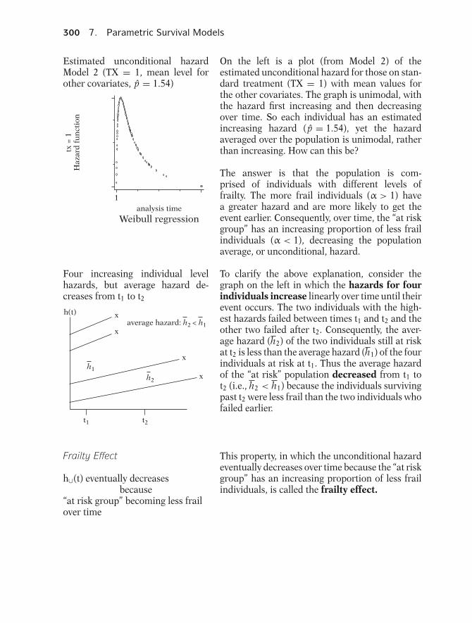
300 7. Parametric Survival Models
Estimated unconditional hazardModel 2 (TX = 1, mean level forother covariates, p = 1.54)
analysis time
Weibull regression
tx =
1H
azar
d f
un
ctio
n
1
On the left is a plot (from Model 2) of theestimated unconditional hazard for those on stan-dard treatment (TX = 1) with mean values forthe other covariates. The graph is unimodal, withthe hazard first increasing and then decreasingover time. So each individual has an estimatedincreasing hazard ( p = 1.54), yet the hazardaveraged over the population is unimodal, ratherthan increasing. How can this be?
The answer is that the population is com-prised of individuals with different levels offrailty. The more frail individuals (α > 1) havea greater hazard and are more likely to get theevent earlier. Consequently, over time, the “at riskgroup” has an increasing proportion of less frailindividuals (α < 1), decreasing the populationaverage, or unconditional, hazard.
Four increasing individual levelhazards, but average hazard de-creases from t1 to t2
h(t)
h1
x
x
x
xh2
t1 t2
average hazard: h2 < h1
To clarify the above explanation, consider thegraph on the left in which the hazards for fourindividuals increase linearly over time until theirevent occurs. The two individuals with the high-est hazards failed between times t1 and t2 and theother two failed after t2. Consequently, the aver-age hazard (h2) of the two individuals still at riskat t2 is less than the average hazard (h1) of the fourindividuals at risk at t1. Thus the average hazardof the “at risk” population decreased from t1 tot2 (i.e., h2 < h1) because the individuals survivingpast t2 were less frail than the two individuals whofailed earlier.
Frailty Effect
h∪(t) eventually decreasesbecause
“at risk group” becoming less frailover time
This property, in which the unconditional hazardeventually decreases over time because the “at riskgroup” has an increasing proportion of less frailindividuals, is called the frailty effect.

Presentation: XII. Frailty Models 301
Unconditional hazard h∪(t) withgamma frailty
h∪(t) = h(t)1 − θ ln[S(t)]
If θ = 0 then h∪(t) = h(t)(no frailty)
The unconditional hazard function h∪(t), withgamma frailty is shown on the left.
If θ = 0, then h∪(t) reduces to h(t) indicating thatthere is no frailty.
For Model 2:
� h(t) and S(t) are Weibull� At t = 0◦ h∪(t) = h(t) (increasing)� As t gets large◦ If θ > 0 then hu(t) → 0� So h∪(t) increases and thendecreases (unimodal)
An examination of the expression for h∪(t) givesfurther insight into how we obtained an estimatedunconditional hazard of unimodal shape. S(t) andh(t) represent the survival and hazard functions ig-noring the frailty, which for Model 2 correspondsto a Weibull distribution. If t = 0 then h∪(t) = h(t),which for Model 2 yields an estimated increasinghazard. As t gets larger, and if θ > 0, the denomi-nator gets larger (because ln[S(t)] is negative) untileventually h∪(t) approaches zero. So h∪(t) is in-creasing at t = 0 but eventually decreases to zero,which means at some point in time, h∪(t) changesdirection.
Population level hazards (withgamma frailty)
h∪1(t) = h1(t)1 − θ ln[S1(t)]
for TX = 1
h∪2(t) = h2(t)1 − θ ln[S2(t)]
for TX = 2
Ratio of unconditional hazards (notPH)
hU 2(t)hU 1(t)
= h2(t)h1(t)
× 1 − θ ln[S1(t)]1 − θ ln[S2(t)]
A consequence of the frailty effect is the need todistinguish between the ratio of individual levelhazards and the ratio of population level haz-ards. For the population level hazards, the PH as-sumption is violated when a gamma (or inverse-Gaussian) distributed frailty is added to a PHmodel. To see this for gamma frailty, let h∪1(t) andh∪2(t) be the unconditional hazard functions rep-resenting the standard and test treatments, respec-tively, at the mean levels of the other covariates.The ratio of these hazards is shown on the left.
302 7. Parametric Survival Models
If
h2(t)h1(t)
= exp(β1)
then
hU 2(t)hU 1(t)
= exp(β1) × 1 − θ ln[S1(t)]1 − θ ln[S2(t)]↗
not constant over time,PH violated
If the ratio of h2(t) and h1(t) equals exp(β1),then the ratio of the unconditional hazards equalsexp(β1) times the ratio of 1 − θ ln[S1(t)] and 1 −θ ln[S2(t)]. This latter ratio is a function of timeand only cancels when t equals zero. Therefore theratio of the unconditional hazards is not constantover time, thus violating the PH assumption.
Plots of S(t)
� Generally averaged overpopulation◦ An important consideration
for frailty models
Generally, survival plots are estimated over a pop-ulation average (e.g., Kaplan–Meier). When con-sidering PH models without frailty, we do not needto distinguish between the conditional and uncon-ditional survival functions. However, this distinc-tion needs to be considered with frailty models.
Suppose ln[−ln S(t)] curves for TXstart parallel but then converge overtime:
1. It may be effect of TX weakensover time
PH model not appropriate2. It may be effect of TX is constant
over time but unobservedheterogeneity is inpopulation
PH model with frailty isappropriate
Suppose we plot Kaplan–Meier log–log survival es-timates evaluating the PH assumption for treat-ment (TX = 2 vs. TX = 1), and the plots start outparallel but then begin to converge over time. Oneinterpretation is that the effect of the treatmentweakens over time. For this interpretation, a PHmodel is not appropriate. Another interpretationis that the effect of the treatment remains con-stant over time but the plots converge due to un-observed heterogeneity in the population. For thisinterpretation, a PH model with frailty would beappropriate.
Model 2 (Weibull with frailty)
� Used PH parameterization� Can equivalently use AFTparameterization
Recall, from Section VI of this chapter, that aWeibull PH model is also an AFT model. The onlydifference is in the way the model is parameter-ized. We next present the AFT form of Model 2.

Presentation: XII. Frailty Models 303
Unconditional survival functionS∪(t) with gamma frailty g(α)
S∪(t) =∞∫
0
S(t |α)g (α)dα
= [[1 − θ ln S(t)]−1/θ
Before stating the model, we show the uncondi-tional survival function using gamma frailty. Re-call that the unconditional survival function is ob-tained by integrating over the frailty, as shown onthe left.
Model 3 (Weibull AFT with gammafrailty)
S∪(t) = [[1 − θ ln S(t)]−1/θ
where S(t) = exp(−λt p) (Weibull)and
1
λ1/p= exp(α0 + α1TX.
+α2PERF + α3DD+α4AGE + α5PRIORTX)
Model 3 (the AFT form of Model 2) is presented interms of the unconditional survival function S∪(t).The unconditional survival function is a functionof S(t), which represents the Weibull survival func-tion. The Weibull survival function, in turn, is pa-rameterized in terms of the shape parameter pand regression coefficients using AFT parameter-ization (see left).
Model 3 Output
Weibull regression (AFT form)Gamma frailtyLog likelihood = −200.11338
t Coef. Std. Err. z P >|z|tx −.068 .190 −0.36 0.721perf .040 .005 8.37 0.000dd .004 .009 0.44 0.661age .008 .009 0.89 0.376priortx .004 .023 0.18 0.860cons 1.460 .752 1.94 0.052
/ln p .435 .141 3.09 0.002/ln the −.150 .382 −0.39 0.695
p 1.54 .2171/p .647 .091theta .861 .329
Likelihood ratio test of theta = 0:
chibar2(01) = 12.18
Prob>=chibar2 = 0.000
γ(TX = 2 vs. 1) = exp(−0.068)= 0.93
Comparing individuals with same α
The output for Model 3, shown on the left, issimilar to that obtained from Model 2. Theestimates for theta and p are identical to thoseobtained from Model 2. The difference is thatthe regression coefficients obtained with Model 3use AFT parameterization (multiply by −p to getthe PH coefficient estimates in Model 2).
An estimated acceleration factor of 0.93 com-paring two individuals with the same level offrailty, for the effect of treatment (TX = 2 vs.TX = 1) and controlling for the other covariates,is obtained by exponentiating the estimatedcoefficient (−0.068) of the TX variable.
304 7. Parametric Survival Models
Interpreting γ
� Taking test treatment reducesindividual’s median survivaltime by factor of 0.93� Suggests slightly harmful effect� α1 is not significant (p = 0.721)
Another interpretation for this estimate is that anindividual taking the test treatment instead of thestandard treatment reduces her median survivaltime (i.e., contracts her individual level survivalfunction) by an estimated factor of 0.93. This esti-mate suggests a slight harmful effect from the testtreatment compared to the standard treatment.However, the estimated coefficient for TX is notsignificant, with a p-value of 0.721.
PH assumptionIndividual level PH ⇒� Populationlevel PH
AFT assumptionIndividual level AFT ⇒ Populationlevel AFT
A key difference between the PH and AFT formu-lations of this model is that if the AFT assump-tion holds at the individual level, then it will alsohold at the population level using the gamma (orinverse-Gaussian) distributed frailty.
Population level survival (withgamma frailty)
S∪1(t) = [[1 − θ ln S1(t)]−1/θ
S∪2(t) = [[1 − θ ln S2(t)]−1/θ
If S1(t) = S2(γt)then
S∪1(t) = [[1 − θ ln S1(t)]−1/θ
= [[1 − θ ln S2(γt)]−1/θ
= S∪2(γt)
Thus,Individual level AFT
⇒ Population level AFT
To see this for gamma frailty, let S∪1(t) and S∪2(t)be the unconditional survival functions represent-ing the standard and test treatments respectively,at the mean levels of the other covariates.
Also let γ represent the individual level accelera-tion factor for treatment; that is, S1(t) = S2(γt).Then S∪1(t) = S∪2(γt) (see left).
Thus, for models with gamma frailty, if the AFT as-sumption holds at the individual level then it alsoholds at the population level.
Presentation: XII. Frailty Models 305
Coefficient estimates from Model 3
� Applies to individual orpopulation� Interpretation of exp(α1) =0.93◦ Median survival time for
individual reduced by factorof 0.93
◦ Median survival timereduced in population byfactor of 0.93
The coefficient estimates obtained from Model 3can therefore be used at the population level aswell as the individual level. So another interpreta-tion for the estimated acceleration factor for treat-ment is that the test treatment reduces the mediansurvival time in the population by an estimatedfactor of 0.93.
Models 2 and 3:Same model, differentparameterizationSame estimates forS(t), S∪(t), h(t), h∪(t)
Model 2 and Model 3 are the same model butuse different parameterizations. The models pro-vide identical estimates for the hazard and survivalfunctions.
Models 2 and 3: Weibull withgamma frailty� Unimodal unconditional hazard
Log-logistic model� Accommodates unimodalhazard without a frailtycomponent
Recall that the estimated unconditional haz-ard function obtained from this frailty model isof unimodal shape. Alternatively, a log-logistic(or lognormal) model, which accommodates aunimodal-shaped hazard function, could havebeen run without the frailty (see Practice Exercises8 to 11 for comparison).
Parametric likelihood with frailty
� Uses f∪(t), where f∪(t) =h∪(t)S∪(t)� Formulated similarly to thatdescribed in Section X with f∪(t)replacing f(t)� Additional parameter θ
The likelihood for Model 3 can be formulated us-ing the unconditional probability density functionf∪(t) which is the product of the unconditionalhazard and survival functions. The likelihood isconstructed in a similar manner to that describedpreviously in this chapter except that f∪(t) is usedfor the likelihood rather than f(t) (see Section X).The main difference is that there is one additionalparameter to estimate, the variance of the frailty.

306 7. Parametric Survival Models
Shared Frailty
� Clusters share same frailty� For example, subjects fromsame family may shareunobserved factors◦ Shared frailty designed to
account for such similarities
Another type of frailty model is the shared frailtymodel. With this model, clusters of subjects areassumed to share the same frailty. For example,subjects from the same family may be similar withrespect to some unobserved genetic or environ-mental factors. Allowing family members to sharethe same frailty is designed to account for suchsimilarities.
Unshared Frailty
� The type of frailty we havedescribed previous to this point� Frailty distributedindependently among subjects
By contrast, the frailty described previous to thispoint (unshared frailty) has been assumed to bedistributed independently among subjects.
Shared Frailty Models
� Similar to random effectregression models� Accounts for within-clustercorrelation� θ is a measure of the degree ofcorrelation
Adding shared frailty to a survival model plays ananalogous role to that of adding a random effect toa linear regression as a way to account for correla-tion between clusters of observations (Kleinbaumand Klein 2002). The estimate for the variance pa-rameter θ in a shared frailty model can be thoughtof as a measure of the degree of correlation, whereθ = 0 indicates no within-cluster correlation.
Hazard conditional on shared frailty(for jth subject in kth cluster)
hjk(t|αk) = αkhjk(t)where
hjk(t) = h(t|Xjk)for j = 1, 2, . . . , nk
and total nk subjects in kth cluster
If family is the cluster variable,then
subjects of same family have sameαk
For a shared frailty model, the conditional hazardfunction for the jth subject from the kth clustercan be expressed as αk multiplied by hjk(t) wherehjk(t) depends on the subject’s covariates Xjk. No-tice that the frailty αk is subscripted by k, but notby j. This indicates that subjects from the samecluster share the same frailty. If, for example, sub-jects are clustered by family, then subjects fromthe same family are assumed to have the samefrailty.

Presentation: XII. Frailty Models 307
Shared and unshared frailty
� Fundamentally the same◦ Accounts for variation due
to unobservable factors� Difference in data to which theyare applied◦ Affects interpretation and
methods of estimation
The frailty in a shared frailty model or unsharedfrailty model is fundamentally the same, a ran-dom effect to account for a source of variation dueto unobservable, or latent, factors. However, thedata to which the shared and unshared frailtyis applied are different, affecting differencesin interpretation and methods of estimation.
Unshared frailty models
� Subjects assumed independent
Shared frailty models
� Accounts for dependenceamong subjects who sharefrailty
For unshared frailty models, a subject’s survival isassumed to be independent of the survival of othersubjects in the study population. For shared frailtymodels, however, the frailty accounts for depen-dence among subjects who share the same frailty.Shared frailty provides an approach to account forcorrelation in the data due to unobservable factorscommon within clusters of subjects.
S∪(t) and h∪(t)
� Population averages inunshared frailty models� Population averages in sharedfrailty models provided thatcluster size is uncorrelated withfrailty
Recall, with unshared frailty models, we inter-preted the unconditional survival and hazardfunctions as representing population averages.With shared frailty models, however, these uncon-ditional functions may not strictly represent pop-ulation averages unless the number of subjects ina cluster is uncorrelated with the level of frailty.
Likelihood for shared frailty models
� More complicated than forunshared frailty models� Unconditional contribution ofeach cluster formulatedseparately by integrating outg(α)� Full likelihood formed asproduct of unconditionalcontribution from each cluster
The formulation of the likelihood is more com-plicated for shared frailty models than it is forunshared frailty models. To construct the sharedfrailty likelihood, the unconditional contributionfor each cluster of subjects is formulated sepa-rately by integrating out the frailty from the prod-uct of each subject’s conditional contribution. Thefull likelihood is then formulated as the product ofthe contributions from each cluster (see Gutierrez2002 for details).
308 7. Parametric Survival Models
Shared frailty in Cox model
� Provided by Stata◦ Only gamma distributed
shared frailty available� Accounts for within-groupcorrelation
Cox shared frailty model
hjk(t|αj) = αkh0(t) exp(βXjk)for j = 1, 2, . . . , nk
total of nk subjects in kth cluster
Up to this point we have discussed frailty in termsof parametric models. Stata (version 8) allowsshared frailty to be included in a Cox model in or-der to account for within-group correlation. Theconditional hazard function for the jth subjectfrom the kth cluster can be expressed as αk mul-tiplied by the baseline hazard h0(t) multiplied byexp(βXjk). The frailty component is assumed tofollow some distribution even though the distribu-tion is unspecified for the rest of the model. Stataonly allows a gamma distribution for the frailty tobe included with a Cox model.
PH violation of h∪(t) in Cox model
� If gamma-distributed frailtyincluded� Interpreting coefficientestimates◦ Only used for HR estimates
among those who sharesame α
If a gamma-distributed frailty component is addedto the Cox model, then the PH assumption is notsatisfied for the unconditional hazards. In thisframework, the frailty in a Cox model can bethought of as a source of random error that causesviolation of the PH assumption at the populationlevel. Consequently, care must be taken in the in-terpretation of the coefficient estimates. They canonly be used to obtain estimates for hazard ratiosconditioned on the same level of frailty.
Recurrent events
� Multiple events from samesubject� Events from same subject maybe correlated� Clusters are formedrepresenting each subject◦ Different subjects do not
share frailty◦ Observations from same
subject share frailty
Shared frailty models can also be applied to re-current event data. It is reasonable to expect thatmultiple events occurring over follow-up from thesame individual would be correlated. To handlewithin-subject correlation, clusters are formed,each containing observations from the same sub-ject. In this setting, it is not the case that differentsubjects share the same frailty. Rather, multipleobservations representing the same subject sharethe same frailty.
Recurrent events:
� Topic of next chapter(Chapter 8)
Survival analyses on recurrent events are the fo-cus of the next chapter (Chapter 8) of this text.An example of a Weibull model with shared frailtyapplied to recurrent event data is presented in thenext chapter.

Presentation: XIII. Summary 309
XIII. Summary
Parametric Models� Assume distribution for survival
time� Distribution specified in termsof parameters� Parameters estimated from data
In this chapter we presented parametric survivalmodels as an alternative to the Cox model. Theyare called parametric models because the distri-bution of the time-to-event variable is specifiedin terms of unknown parameters, which are esti-mated from the data. Distributions that are com-monly utilized are the exponential, the Weibull,the log-logistic, the lognormal, and the general-ized gamma.
f(t) specified ⇒ corresponding S(t),h(t) also determined
Moreover,Specifying one of f(t), S(t), or h(t)determines all three functions
More precisely, for parametric survival models, itis the probability density function f(t) of the dis-tribution that is specified in terms of the parame-ters. Once f(t) is specified, the corresponding sur-vival and hazard functions S(t) and h(t) can also bedetermined. Moreover, specifying any one of theprobability density function, survival function, orhazard function allows the other two functions tobe determined.
Parametric models
� Need not be PH models� Many are AFT models
The proportional hazards (PH) assumption is theunderlying assumption for a Cox PH model. How-ever, parametric survival models need not be pro-portional hazards models. Many parametric mod-els are acceleration failure time (AFT) modelsrather than proportional hazards models.
Acceleration factor (γ)
� Key measure of association inAFT models� Describes stretching orcontraction of S(t)
AFT assumptionS2(t) = S1(γt)↑ ↑
Group 2 Group 1
The acceleration factor (γ) is the key measureof association obtained in an AFT model. It de-scribes the “stretching out” or contraction of sur-vival functions when comparing one group to an-other. If S1(t) and S2(t) are the survival func-tions for Group 1 and Group 2, respectively, thenthe AFT assumption can be expressed as S2(t) =S1(γt).
Detailed examples presented:
� Exponential model� Weibull model� Log-logistic model
We presented detailed examples of the exponen-tial, Weibull, and log-logistic model using the re-mission dataset.
310 7. Parametric Survival Models
Exponential Model
� h(t) = λ (constant hazard)� Special case of Weibull model
Weibull Model
� AFT PH
Log-logistic Model
� Not a PH model� AFT PO
The underlying assumption for an exponentialmodel, a special case of the Weibull model, is thatthe hazard function is constant over time (i.e.,h(t) =λ). The Weibull model is unique in that if thePH assumption holds then the AFT assumptionalso holds (and vice versa). The log-logistic modeldoes not accommodate the PH assumption. How-ever, if the AFT assumption holds in a log-logisticmodel, then the proportional odds (PO) assump-tion also holds (and vice versa).
PO assumption
OR = S(t, x∗)/[1 − S(t, x∗)]S(t, x)/[1 − S(t, x)]
OR is constant over time
The idea underlying the proportional odds as-sumption is that the survival (or failure) odds ra-tio comparing two specifications of covariates re-mains constant over time.
Graphical Evaluation
Weibull and Exponential
� Plot ln[−ln S(t)] against ln(t)
Log-logistic:
� Plot ln[
S(t)(1−S(t))
]against ln(t).
Check for linearity
We presented graphical approaches for evaluatingthe appropriateness of the exponential, Weibull,and log-logistic model by plotting a function ofthe Kaplan–Meier survival estimates S(t) againstthe log of time and then checking for linearity.
For evaluation of the exponential and Weibullassumptions, the ln[− ln S(t)] is plotted againstln(t) and for evaluation of the log-logistic as-sumption the log odds of S(t) is plotted againstln(t).
Presented other parametric models
� Generalized gamma model� Lognormal model� Gompertz model
We briefly discussed other parametric modelssuch as the generalized gamma, lognormal, andGompertz models and showed additional para-metric approaches such as modeling ancillary(shape) parameters as a function of predictor vari-ables.

Presentation: XIII. Summary 311
Contributions to Likelihood
If event at t, contributes f(t)
If censored, integrate over f(t)t1∫
0
f (t)dt: left-censored at t1
∞∫t1
f (t)dt: right-censored at t1
t2∫t1
f (t)dt: interval-censoredfrom t1 to t2
The parametric likelihood was developed and in-cludes a discussion of left-, right-, and interval-censored data. If a subject has an event at time t,then that subject’s contribution to the likelihoodis f(t). On the other hand, if a subject is censored(i.e., exact time of event unknown), then the sub-ject’s contribution to the likelihood is found by in-tegrating over f(t). The integration limits are de-termined by the time and type of censorship (seeleft).
Full likelihood (L)
L =N∏
j=1
L j j = 1, 2, . . . , N
where L j is the contribution fromjth subject
Assuming independence among subjects, the fulllikelihood can be formulated as a product of eachsubject’s contribution.
Binary regression for interval-censored data
� Follow-up divided into intervals◦ Allows for multiple
observations per subject� Binary outcome variabledefined◦ Indicates survival or failure
over each interval
We showed how binary regression could be ap-plied to interval-censored data by defining a di-chotomous outcome variable indicating subjects’survival or failure over each interval of theirfollow-up. The data layout for this type of anal-ysis allows multiple observations per subject, rep-resenting intervals of survival prior to failure (orcensorship).
Binary regression for discrete sur-vival analysis
� Analogous to interval-censoreddata◦ Discrete outcome—subjects
survive discrete units of time◦ Interval outcomes—
subjects survive intervalsof time
Binary regression can also be used for discrete sur-vival analysis in which the “time-to-event” variableis considered discrete rather than continuous. Thedata layout is similar to that for interval-censoreddata except subjects are conceptualized as surviv-ing discrete units of time rather than continuousintervals of time.

312 7. Parametric Survival Models
Frailty, α
h(t|α) = αh(t)
↗multiplicative effect on h(t)mean = 1, variance = θ
θ estimated from data
We concluded with a discussion of frailty mod-els. The frailty α is a multiplicative random effecton the hazard designed to account for individual-level unobserved factors that add an extra layer ofvariability beyond what has already been specifiedin the model. The frailty is generally assumed tofollow a distribution with mean equal to 1 and istypically parameterized in terms of the variance θ
which is estimated from the data.
Chapters
1. Introduction to SurvivalAnalysis
2. Kaplan–Meier Curves and theLog-Rank Test
3. The Cox Proportional HazardModel
4. Evaluating the ProportionalHazards Assumption
5. The Stratified Cox Procedure6. Extension of the Cox
Proprtional Hazards Model forTime-Dependent Covariates
✓7. Parametric Survival Models
The presentation is now complete. The readercan review the detailed outline that follows andthen answer the practice exercises and test.
In the next chapter (8) entitled “RecurrentEvent Survival Analysis,” we consider approachesfor analyzing data in which individuals may havemore than one event over the course of theirfollow-up.
Next:
8. Recurrent Event SurvivalAnalysis

Detailed Outline 313
DetailedOutline
I. Overview (pages 260–262)A. Parametric Survival Models
i. Outcome assumed to follow specifieddistribution
ii. Weibull, exponential (a special case of theWeibull), log-logistic, lognormal, andgeneralized gamma are supported withpopular software (SAS and Stata)
iii. Contrasts with Cox model in which baselinehazard and survival functions are not specified
II. Probability Density Function in Relation to theHazard and Survival Function (pages 262–263)A. If any one of the hazard h(t), survival s(t), or
probability density f(t) functions is known thenthe other two functions can be determined.
B. If f(t) is specified, then S(t) =∞∫
t
f (u)du
C. If S(t) is specified, thenh(t) = (−d[S(t)]/dt)/S(t) andf (t) = (−d[S(t)])/dt
D. If h(t) is specified, then S(t) = exp(−t∫
0
h(u)du)
and f (t) = h(t)S(t)III. Exponential Example (pages 263–265)
A. Hazard is constant (i.e., not a function of time) inan exponential modeli. Stronger assumption than the PH assumption
that the HR is constantB. Exponential PH model (one predictor X1)
i. In terms of the hazard: h(t) = λ whereλ = exp(β0 + β1X1)
ii. Hazard ratio: HR (X1 = 1 vs. X1 = 0) = exp(β1)IV. Acceleration Failure Time Assumption
(pages 266–268)A. Underlying assumptions
i. AFT—effect of covariates is multiplicative withrespect to survival time
ii. PH—effect of covariates is multiplicative withrespect to the hazard
314 7. Parametric Survival Models
B. The acceleration factor (γ) is the key measureof association in an AFTi. Acceleration factor is a ratio of survival times
corresponding to any fixed value of S(t), thatis, tA/tB where A and B denote two individualsfor which S(tA) = S(tB)
ii. S2(t) = S1(γt), survival function for Group 1,S1(t) is stretched (or contracted) by a factor ofγ compared to survival function for Group 2,S2(t)
C. AFT illustrationi. Dogs are said to grow older 7 times faster
than humans, SD(t) = SH(7t)V. Exponential Example Revisited (pages 268–272)
A. Exponential AFT model (one predictor X1)i. In terms of survival: S(t) = exp(−λt) where
λ = exp[−(α0 + α1 X1)]ii. In terms of time:
t = [−ln(S(t)] × exp(α0 + α1X1)iii. Acceleration factor (X1 = 1 vs.
X1 = 0),γ = exp(α1)B. An exponential PH model is an exponential AFT
model (but uses different parameterization)i. βj = −αj, where βj and αj are PH and AFT
parameterization for the jth covariateii. α > 1 for (X1 = 1 vs. X1 = 0) implies effect
of X1 = 1 is beneficial to survivaliii. HR > 1 for (X1 = 1 vs. X1 = 0) implies effect
of X1 = 1 is harmful to survivalC. Exponential model is a special case of a Weibull
modeli. Graphical approach for evaluating
appropriateness of exponential model isdescribed in the section on the Weibullexample
VI. Weibull Example (pages 272–277)A. PH form of the Weibull model (one predictor X1)
i. In terms of the hazard: h(t) = λpt p−1 whereλ = exp(β0 + β1X1)
ii. Hazard ratio: HR (X1 = 1 vs.X1 = 0) = exp(β1)

Detailed Outline 315
iii. Weibull hazard is monotonic with itsdirection determined by the value of theshape parameter pa. p > 1 hazard increases over timeb. p = 1 constant hazard (exponential model)c. p < 1 hazard decreases over time
A. Graphical approach for evaluating appropriatenessof Weibull modeli. Plot the log negative log of the Kaplan–Meier
survival estimates against the log of time foreach pattern of covariatesa. If Weibull assumption is correct then plots
should be straight lines of slope pb. If exponential assumption is correct then
plots should be straight lines with slopeequal to one (p = 1)
c. If plots are parallel straight lines thenWeibull PH and AFT assumptions arereasonable
B. AFT form of the Weibull model (one predictor X1)i. In terms of survival:
S(t) = exp(−λt p) = exp[−(λ1/pt)p] whereλ1/p = exp[−(α0 + α1X1)]
ii. In terms of time:t = [−ln(S(t)]1/p × exp(α0 + α1X1)
iii. Acceleration factor (X1 = 1 vs. X1 = 0),γ = exp(α1)
C. A Weibull PH model is a Weibull AFT model (butuses different parameterization)i. Unique property of Weibull model
(exponential is special case, p = 1)ii. βj = −αj p where βj and αj are PH and AFT
parameterization, respectively, for the jthcovariate
VII. Log-Logistic Example (pages 277–282)A. Log-logistic hazard function:
h(t) = λpt p−1/(1 + λt p).i. p ≤ 1 hazard decreases over time
ii. p > 1 hazard first increases and thendecreases over time (unimodal)

316 7. Parametric Survival Models
B. Graphical approach for evaluatingappropriateness of log-logistic modeli. Plot the log of the survival odds (using KM
estimates) against the log of time for eachpattern of covariatesa. If log-logistic assumption is correct then
plots should be straight line of slope −pb. If plots are parallel straight lines then
log-logistic proportional odds (PO) and AFTassumptions are reasonable
C. Log-logistic AFT model (one predictor X1):i. In terms of survival:
S(t) = 1/(1 + λt p) = 1/(1 + (λ1/pt)p)where λ1/p = exp(−(α0 + α1X1))
ii. In terms of time:
t =[
1S(t) − 1
]1/p× exp(α0 + α1X1)
iii. Acceleration factor (X1 = 1 vs. X1 = 0),γ = exp(α1)
D. Log-logistic proportional odds (PO) model(one predictor X1)
i. In terms of survival: S(t) = 1/(1 + λt p) whereλ = exp(β0 + β1X1)
ii. Odds of an event (failure odds) by time t:(1 − S(t))/S(t) = λt p
iii. Odds of surviving event (survival odds)beyond t: S(t)/(1 − S(t)) = 1/λt p
iv. Failure odds ratio:HR (X1 = 1 vs. X1 = 0) = exp(β1)a. PO assumption is that the odds ratio is
constant over timev. Survival odds ratio:
HR (X1 = 1 vs. X1 = 0) = exp(−β1)a. Survival odds ratio is reciprocal of failure
odds ratioE. A log-logistic AFT model is a log-logistic PO
model (but uses different parameterization)i. Log-logistic model is not a proportional
hazards (PH) modelii. βj = −αj p where βj and αj are PO and AFT
parameterization for the jth covariatea. Shape parameter with Stata is
parameterized as gamma = 1/p
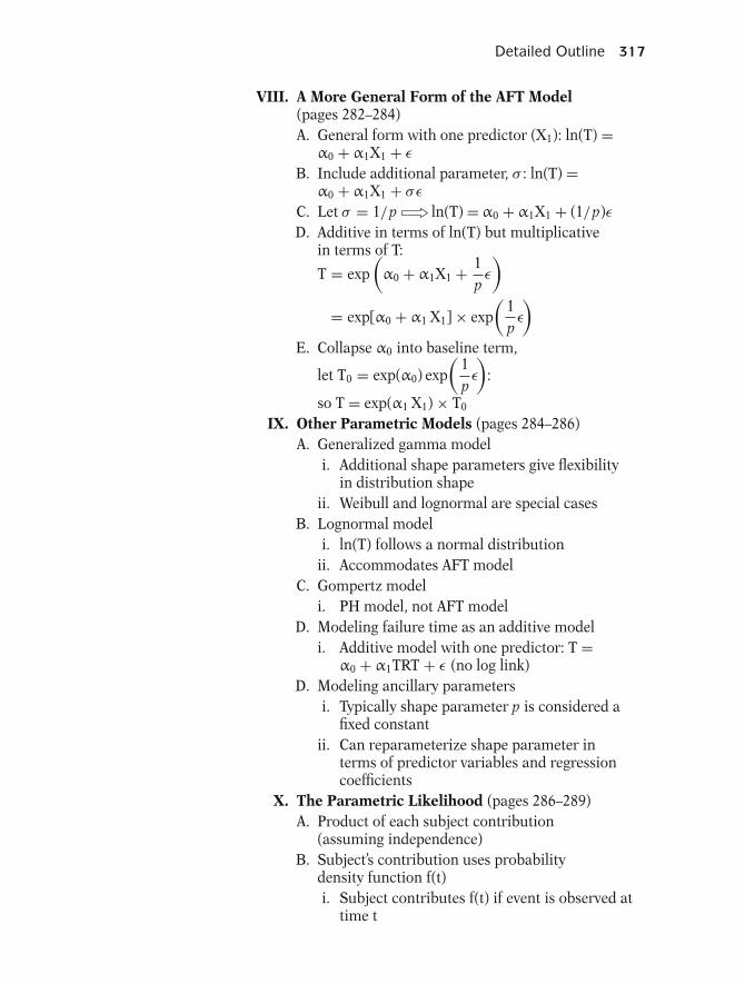
Detailed Outline 317
VIII. A More General Form of the AFT Model(pages 282–284)A. General form with one predictor (X1): ln(T) =
α0 + α1X1 + ε
B. Include additional parameter, σ : ln(T) =α0 + α1X1 + σε
C. Let σ = 1/p ln(T) = α0 + α1X1 + (1/p)εD. Additive in terms of ln(T) but multiplicative
in terms of T:
T = exp(α0 + α1X1 + 1
pε
)= exp[α0 + α1 X1] × exp
(1pε
)E. Collapse α0 into baseline term,
let T0 = exp(α0) exp(
1pε
):
so T = exp(α1 X1) × T0
IX. Other Parametric Models (pages 284–286)A. Generalized gamma model
i. Additional shape parameters give flexibilityin distribution shape
ii. Weibull and lognormal are special casesB. Lognormal model
i. ln(T) follows a normal distributionii. Accommodates AFT model
C. Gompertz modeli. PH model, not AFT model
D. Modeling failure time as an additive modeli. Additive model with one predictor: T =
α0 + α1TRT + ε (no log link)D. Modeling ancillary parameters
i. Typically shape parameter p is considered afixed constant
ii. Can reparameterize shape parameter interms of predictor variables and regressioncoefficients
X. The Parametric Likelihood (pages 286–289)A. Product of each subject contribution
(assuming independence)B. Subject’s contribution uses probability
density function f(t)i. Subject contributes f(t) if event is observed at
time t

318 7. Parametric Survival Models
ii. Integrate over f(t) if subject is censoreda. Integrate from 0 to t if subject is
left-censored at tb. Integrate from t to infinity if subject is
right-censored at tc. Integrate over interval of censorship if
subject is interval-censoredXI. Interval-Censored Data (pages 289–294)
A. Binary regression is alternative approach ifdata are interval-censored
B. Binary outcome variable represents survivalor failure over each subinterval of subject’sfollow-up
C. Specify a link function when using binaryregressioni. Logit link for logistic regression
ii. Complementary log–log link is an alternativeto logistic regression
D. Discrete survival analysisi. Time-to-event variable is discrete
ii. Binary regression can be applied in a similarmanner to that of interval-censored data
XII. Frailty Models (pages 294–308)A. The frailty α is an unobserved multiplicative
effect on the hazard functioni. Hazard, conditioned on the frailty,
h(t|α) = αh(t)ii. Survival, conditioned on the frailty,
S(t|α) = S(t)α
B. Frailty assumed to follow some distributiong(α) of mean 1 and variance θ
i. The variance θ is a parameter estimated bythe data
ii. Gamma and inverse-Gaussian aredistributions offered by Stata software
C. Designed to account for unobservedindividual-level factors that influence survivali. Distinction is made between the
individual-level and population-level hazards.PH assumption may hold on individual levelbut not on population level

Practice Exercises 319
D. Shared frailty models allow individuals toshare the same frailtyi. Play similar role as adding a random effect to
a linear regressionii. Can account for within-group correlation.
XIII. Summary (pages 309–312)
PracticeExercises
Answer questions 1 to 5 as true or false (circle T or F)
T F 1. The acceleration factor comparing exposed andunexposed subjects, (E = 1 vs. E = 0), is a ratioof their median survival times (time to S(t) = 0.5),or more generally the ratio of their times to anyfixed value of S(t) = q.
T F 2. Let S0(t) be the survival function for unexposedsubjects (E = 0) and let S1(t) be the survival func-tion for exposed subjects (E = 1). If S0(t) = S1(3t)then the median survival time for the unexposedsubjects is 3 times longer than the median survivaltime for the exposed subjects.
T F 3. The Cox proportional hazards model is a paramet-ric model.
T F 4. If the acceleration failure time (AFT) assumptionholds in a Weibull model then the proportional haz-ards assumption also holds.
T F 5. The hazard is assumed constant in a log-logisticmodel.
Questions 6 and 7 make use of the output (copied below) pre-sented in Sections III and V containing an example of the ex-ponential model. This example used the remission data withtreatment status (coded TRT = 1 for the experimental treat-ment and TRT = 0 for the placebo). The exponential survivaland hazard functions are, respectively, S(t) = exp(−λt) andh(t) = λ where λ = exp[−(α0 + α1TRT)] for the AFT param-eterization and λ = exp(β0 + β1TRT) for the PH parameter-ization. The output for both the AFT and PH forms of themodel are presented.
Exponential regressionaccelerated failure-time formλ = exp[−(α0 + α1TRT)]
t Coef. Std. Err. z p >|z|trt 1.527 .398 3.83 0.00
cons 2.159 .218 9.90 0.00
Exponential regression logrelative-hazard formλ = exp(β0 + β1TRT)
t Coef. Std. Err. z p >|z|trt −1.527 .398 3.83 0.00
cons −2.159 .218 −9.90 0.00
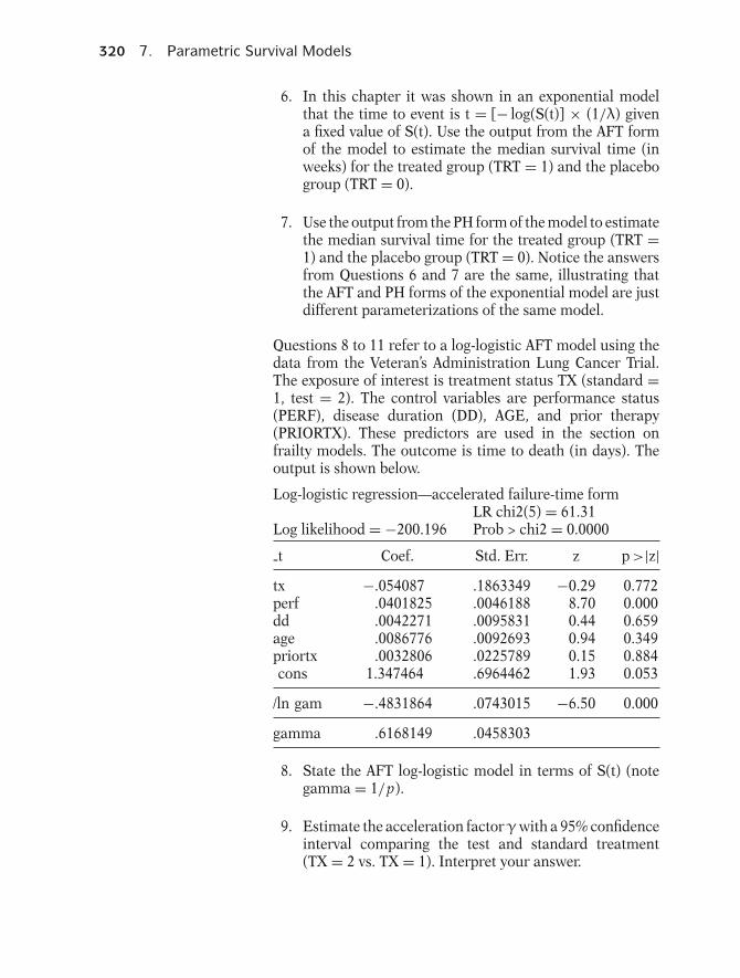
320 7. Parametric Survival Models
6. In this chapter it was shown in an exponential modelthat the time to event is t = [− log(S(t)] × (1/λ) givena fixed value of S(t). Use the output from the AFT formof the model to estimate the median survival time (inweeks) for the treated group (TRT = 1) and the placebogroup (TRT = 0).
7. Use the output from the PH form of the model to estimatethe median survival time for the treated group (TRT =1) and the placebo group (TRT = 0). Notice the answersfrom Questions 6 and 7 are the same, illustrating thatthe AFT and PH forms of the exponential model are justdifferent parameterizations of the same model.
Questions 8 to 11 refer to a log-logistic AFT model using thedata from the Veteran’s Administration Lung Cancer Trial.The exposure of interest is treatment status TX (standard =1, test = 2). The control variables are performance status(PERF), disease duration (DD), AGE, and prior therapy(PRIORTX). These predictors are used in the section onfrailty models. The outcome is time to death (in days). Theoutput is shown below.
Log-logistic regression—accelerated failure-time formLR chi2(5) = 61.31
Log likelihood = −200.196 Prob > chi2 = 0.0000
t Coef. Std. Err. z p >|z|tx −.054087 .1863349 −0.29 0.772perf .0401825 .0046188 8.70 0.000dd .0042271 .0095831 0.44 0.659age .0086776 .0092693 0.94 0.349priortx .0032806 .0225789 0.15 0.884cons 1.347464 .6964462 1.93 0.053
/ln gam −.4831864 .0743015 −6.50 0.000
gamma .6168149 .0458303
8. State the AFT log-logistic model in terms of S(t) (notegamma = 1/p).
9. Estimate the acceleration factor γ with a 95% confidenceinterval comparing the test and standard treatment(TX = 2 vs. TX = 1). Interpret your answer.

Practice Exercises 321
10. The AFT log-logistic model is also a proportional oddsmodel. Use the output to estimate the odds ratio (oddsof death) comparing the test and standard treatment.Also estimate the survival odds ratio comparing the testand standard treatment.
11. The Akaike Information Criterion (AIC) is a method de-signed to compare the fit of different models. For thisquestion, three models are compared using the same 5predictors:1. A Weibull model without frailty (presented as Model
1 in the section on frailty models);2. A Weibull model containing a frailty component (pre-
sented as Model 2 in the section on frailty models);and
3. The log-logistic model presented above.
Below is a table containing the log likelihood statistic foreach model.
Number ofModel Frailty parameters Log likelihood
1. Weibull No 7 −206.2042. Weibull Yes 8 −200.1933. Log-logistic No 7 −200.196
The goal for this question is to calculate the AIC statisticfor each model and select the model based on this criterion.The AIC statistic is calculated as: −2 log likelihood +2p (where p is the number of parameters in the model). Asmaller AIC statistic suggests a better fit. The addition of2 times p can be thought of as a penalty if nonpredictiveparameters are added to the model. Each model containsthe 5 predictors, an intercept, and a shape parameter.Model 2 contains an additional variance parameter (theta)because a frailty component is included in the model.The log likelihood was unchanged when a frailty compo-nent was added to the log-logistic model (not shown in table).
Note that if we are just comparing Models 1 and 2 wecould use the likelihood ratio test because Model 1 is nested(contained) in Model 2. The likelihood ratio test is considereda superior method to the AIC for comparing models butcannot be used to compare the log-logistic model to theother two, because that model uses a different distribution.
Which of the three models should be selected based onthe AIC?

322 7. Parametric Survival Models
Questions 12 to 14 refer to a generalized gamma model us-ing the Veterans’ data with the same five predictor variablesthat were used in the model for Questions 8 to 10. The gen-eralized gamma distribution contains two shape parameters(kappa and sigma) that allow great flexibility in the shape ofthe hazard. If kappa = 1, the model reduces to a Weibull dis-tribution with p = 1/sigma. If kappa = 0 the model reducesto a lognormal distribution. The output is shown below.
Gamma regression—accelerated failure-time formLR chi2(5) = 52.86
Log likelihood = −200.626 Prob > chi2 = 0.0000
t Coef. Std. Err. z p >|z|tx −.131 .1908 −0.69 0.491perf .039 .0051 7.77 0.000dd .0004 .0097 0.04 0.965age .008 .0095 0.89 0.376priortx .004 .0229 0.17 0.864cons 1.665 .7725 2.16 0.031
/ln sig .0859 .0654 1.31 0.189/kappa .2376 .2193 1.08 0.279
sigma 1.0898 .0714
12. Estimate the acceleration factor γ with a 95% confidenceinterval comparing the test and standard treatment (TX= 2 vs. TX = 1).
13. Use the output to test the null hypothesis that a lognor-mal distribution is appropriate for this model.
14. A lognormal model was run with the same five predic-tors (output not shown) and yielded very similar param-eter estimates to those obtained from the generalizedgamma model shown above. The value of the log likeli-hood for the lognormal model was −201.210. Comparethe AIC of the generalized gamma model, the lognormalmodel, and the log-logistic model from Question 11 andselect a model based on that criterion. Note: each modelcontains an intercept and five predictors. The general-ized gamma distribution contains two additional shapeparameters and the log-logistic and lognormal distribu-tions each contain one additional shape parameter (seeQuestion 11 for further details on the AIC).

Practice Exercises 323
Questions 15 to 17 refer to a Weibull model using theremission data with treatment as the only predictor (codedTRT = 1 for the test treatment and TRT = 0 for the placebo).In this model both λ and p are modeled as functions ofthe predictor TRT. The model can be stated in terms of thehazard function: h(t) = λpt p−1 where λ = exp(β0 + β1TRT)and p = exp(δ0 + δ1TRT). Typically, the shape parameter ina Weibull model is assumed constant (i.e., δ1 = 0) acrosslevels of covariates. This model is discussed in the section ofthis chapter called “Other Parametric Models.” The outputobtained using Stata is shown below.
Weibull regression—log relative-hazard formLR chi2(1) = 1.69
Log likelihood = −47.063396 Prob > chi2 = 0.1941
t Coef. Std. Err. z p >|z|t
trt −1.682 1.374 −1.22 0.221cons −3.083 .646 −4.77 0.000
ln ptrt −.012 .328 −0.04 0.970cons .315 .174 1.82 0.069
15. Even though λ is parameterized similarly to that in a PHWeibull model, this model is not a PH model becausethe shape parameter p varies across treatment groups.Show the PH assumption is violated in this model byestimating the hazard ratios for TRT = 0 vs. TRT = 1after 10 weeks and after 20 weeks of follow-up.
16. Perform a statistical test on the hypothesis δ1 = 0 (thecoefficient for the treatment term for ln(p)). Note: if weassume δ1 = 0, then the model reduces to the exampleof the Weibull PH model presented in Section VI of thischapter.
17. Consider the plot of the log negative log of the Kaplan–Meier survival estimates against the log of time forTRT = 1 and TRT = 0. How should the graph look ifδ1 = 0?
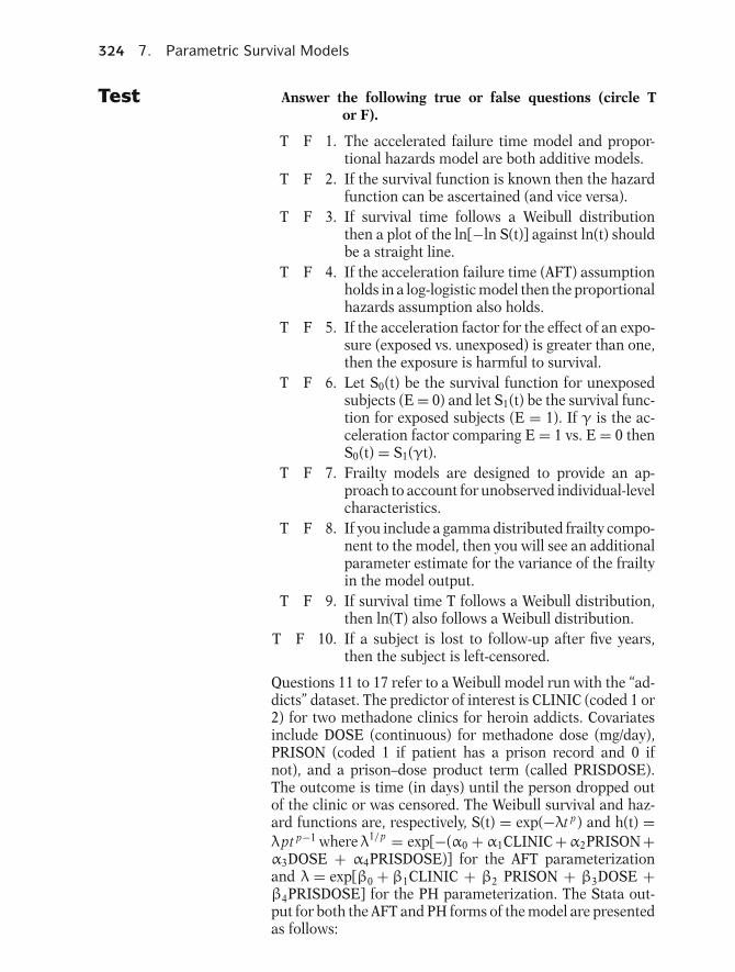
324 7. Parametric Survival Models
Test Answer the following true or false questions (circle Tor F).
T F 1. The accelerated failure time model and propor-tional hazards model are both additive models.
T F 2. If the survival function is known then the hazardfunction can be ascertained (and vice versa).
T F 3. If survival time follows a Weibull distributionthen a plot of the ln[−ln S(t)] against ln(t) shouldbe a straight line.
T F 4. If the acceleration failure time (AFT) assumptionholds in a log-logistic model then the proportionalhazards assumption also holds.
T F 5. If the acceleration factor for the effect of an expo-sure (exposed vs. unexposed) is greater than one,then the exposure is harmful to survival.
T F 6. Let S0(t) be the survival function for unexposedsubjects (E = 0) and let S1(t) be the survival func-tion for exposed subjects (E = 1). If γ is the ac-celeration factor comparing E = 1 vs. E = 0 thenS0(t) = S1(γt).
T F 7. Frailty models are designed to provide an ap-proach to account for unobserved individual-levelcharacteristics.
T F 8. If you include a gamma distributed frailty compo-nent to the model, then you will see an additionalparameter estimate for the variance of the frailtyin the model output.
T F 9. If survival time T follows a Weibull distribution,then ln(T) also follows a Weibull distribution.
T F 10. If a subject is lost to follow-up after five years,then the subject is left-censored.
Questions 11 to 17 refer to a Weibull model run with the “ad-dicts” dataset. The predictor of interest is CLINIC (coded 1 or2) for two methadone clinics for heroin addicts. Covariatesinclude DOSE (continuous) for methadone dose (mg/day),PRISON (coded 1 if patient has a prison record and 0 ifnot), and a prison–dose product term (called PRISDOSE).The outcome is time (in days) until the person dropped outof the clinic or was censored. The Weibull survival and haz-ard functions are, respectively, S(t) = exp(−λt p) and h(t) =λpt p−1 where λ1/p = exp[−(α0 + α1CLINIC +α2PRISON +α3DOSE + α4PRISDOSE)] for the AFT parameterizationand λ = exp[β0 + β1CLINIC + β2 PRISON + β3DOSE +β4PRISDOSE] for the PH parameterization. The Stata out-put for both the AFT and PH forms of the model are presentedas follows:

Test 325
Weibull regressionaccelerated failure-time form
Log likelihood = −260.74854
t Coef. Std. Err. z p >|z|clinic .698 .158 4.42 0.000prison .145 .558 0.26 0.795dose .027 .006 4.60 0.000prisdose −.006 .009 −0.69 0.492cons 3.977 .376 10.58 0.000
/ln p .315 .068 4.67 0.000
p 1.3704671/p .729678
Weibull regressionlog relative-hazard form
Log likelihood = −260.74854
t Coef. Std. Err. z p >|z|clinic −.957 .213 −4.49 0.000prison −.198 .765 −0.26 0.795dose −.037 .008 −4.63 0.000prisdose .009 .013 0.69 0.491cons −5.450 .702 −7.76 0.000
/ln p .315 .068 4.67 0.000
p 1.3704671/p .729678
11. Estimate the acceleration factor with a 95% confidenceinterval comparing CLINIC = 2 vs. CLINIC = 1. Interpretthis result.
12. Estimate the hazard ratio with a 95% confidence intervalcomparing CLINIC = 2 vs. CLINIC = 1. Interpret thisresult.
13. Estimate the coefficient for CLINIC in the PH Weibullmodel using the results reported in the output fromthe AFT form of the model. Hint: the coefficients for aWeibull PH and AFT model are related β j = −α j p forthe jth covariate.
14. Is the product term PRISDOSE included in the model toaccount for potential interaction or potential confound-ing of the effect of CLINIC on survival?
15. Use the output to estimate the median survival time fora patient from CLINIC = 2 who has a prison record andreceives a methadone dose of 50 mg/day. Hint: use the re-lationship that t = [−ln S(t)]1/p × (1/λ1/p) for a Weibullmodel.
16. Use the output to estimate the median survival time fora patient from CLINIC = 1 who has a prison record andreceives a methadone dose of 50 mg/day.
17. What is the ratio of your answers from Questions 15and 16 and how does this ratio relate to the accelerationfactor?
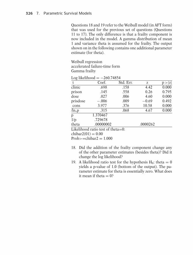
326 7. Parametric Survival Models
Questions 18 and 19 refer to the Weibull model (in AFT form)that was used for the previous set of questions (Questions11 to 17). The only difference is that a frailty component isnow included in the model. A gamma distribution of mean1 and variance theta is assumed for the frailty. The outputshown on in the following contains one additional parameterestimate (for theta).
Weibull regressionaccelerated failure-time formGamma frailty
Log likelihood = −260.74854t Coef. Std. Err. z p >|z|
clinic .698 .158 4.42 0.000prison .145 .558 0.26 0.795dose .027 .006 4.60 0.000prisdose −.006 .009 −0.69 0.492cons 3.977 .376 10.58 0.000
/ln p .315 .068 4.67 0.000p 1.3704671/p .729678theta .00000002 .0000262Likelihood ratio test of theta=0:chibar2(01) = 0.00Prob>=chibar2 = 1.000
18. Did the addition of the frailty component change anyof the other parameter estimates (besides theta)? Did itchange the log likelihood?
19. A likelihood ratio test for the hypothesis H0: theta = 0yields a p-value of 1.0 (bottom of the output). The pa-rameter estimate for theta is essentially zero. What doesit mean if theta = 0?

Answers to Practice Exercises 327
Answers toPracticeExercises
1. T
2. F: The median survival time for the unexposed is 1/3 of themedian survival time for the exposed.
3. F: The Cox model is a semiparametric model. The distri-bution of survival time is unspecified in a Cox model.
4. T
5. F: The hazard is assumed constant in an exponentialmodel.
6. t = [−log(S(t)] × (1/λ), where S(t) = 0.5, and 1/λ =exp(α0 + α1TRT).For TRT = 0: estimated median survival
= [−ln(0.5)] exp(2.159) = 6.0 weeks.For TRT = 1: estimated median survival
= [−ln(0.5)] exp(2.159 + 1.527) = 27.6 weeks.
7. t = [−log(S(t)] (1/λ), where S(t) = 0.5, andλ = exp(β0 + β1TRT) ⇒ 1/λ = exp[−(β0 + β1TRT)].For TRT = 0: estimated median survival
= [−ln(0.5)] exp[−(−2.159)] = 6.0 weeks.For TRT = 1: estimated median survival
= [−ln(0.5)] exp[−(−2.159 − 1.527)] = 27.6 weeks.
8. S(t) = 1/(1 + λt p) where λ1/p = exp[−(α0 + α1TX+ α2PERF + α3DD + α4AGE + α5PRIORTX)].
9. γ = exp[α0 + α1(2) + α2PERF + α3 D D + α4 AG E + α5PRIORTX]exp[α0 + α1(1) + α2PERF + α3 D D + α4 AG E + α5PRIORTX]
= exp(α1)
γ = exp(−0.054087) = 0.95
95% CI = exp[−0.054087 ± 1.96(0.1863349)] = (0.66, 1.36)
The point estimate along with the 95% CI suggests a nullresult.
10. The coefficients for a log-logistic proportional odds (PO)and AFT model are related β1 = −α1 p = −β1÷ gamma,where β1 is the coefficient for TX in a PO model.OR = exp(−α1÷ gamma)estimated OR = exp(−0.054087 ÷ 0.6168149) = 0.92estimated survival OR = 1/[exp(−0.054087 ÷ 0.6168149)]
= 1.09.
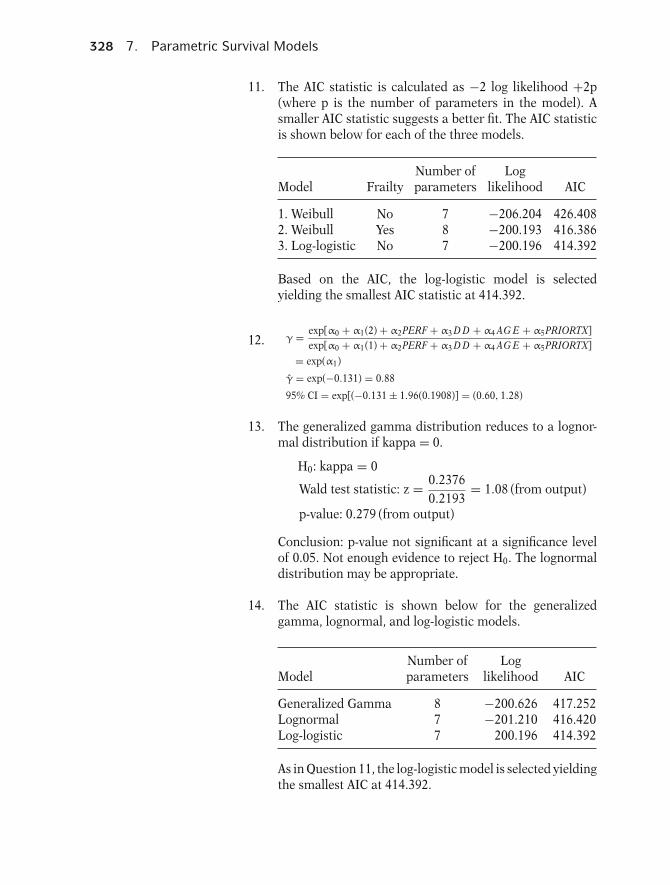
328 7. Parametric Survival Models
11. The AIC statistic is calculated as −2 log likelihood +2p(where p is the number of parameters in the model). Asmaller AIC statistic suggests a better fit. The AIC statisticis shown below for each of the three models.
Number of LogModel Frailty parameters likelihood AIC
1. Weibull No 7 −206.204 426.4082. Weibull Yes 8 −200.193 416.3863. Log-logistic No 7 −200.196 414.392
Based on the AIC, the log-logistic model is selectedyielding the smallest AIC statistic at 414.392.
12. γ = exp[α0 + α1(2) + α2PERF + α3 D D + α4 AG E + α5PRIORTX]exp[α0 + α1(1) + α2PERF + α3 D D + α4 AG E + α5PRIORTX]
= exp(α1)
γ = exp(−0.131) = 0.88
95% CI = exp[(−0.131 ± 1.96(0.1908)] = (0.60, 1.28)
13. The generalized gamma distribution reduces to a lognor-mal distribution if kappa = 0.
H0: kappa = 0
Wald test statistic: z = 0.23760.2193
= 1.08 (from output)
p-value: 0.279 (from output)
Conclusion: p-value not significant at a significance levelof 0.05. Not enough evidence to reject H0. The lognormaldistribution may be appropriate.
14. The AIC statistic is shown below for the generalizedgamma, lognormal, and log-logistic models.
Number of LogModel parameters likelihood AIC
Generalized Gamma 8 −200.626 417.252Lognormal 7 −201.210 416.420Log-logistic 7 200.196 414.392
As in Question 11, the log-logistic model is selected yieldingthe smallest AIC at 414.392.

Answers to Practice Exercises 329
15. h(t) = λpt p−1 where λ = exp(β0 + β1TRT) andp = exp(δ0 + δ1TRT)let λ0 = exp[β0 + β1(0)], λ1 = exp[β0 + β1(1)]
let p0 = exp[δ0 + δ1(0)], p1 = exp[δ0 + δ1(1)]
λ0 = 0.0458, λ1 = 0.0085, p0 = 1.3703,
p1 = 1.3539 (calculated using output)
HR (TRT = 0 vs. TRT = 1) = λ0 p0t p0−1
λ1 p1t p1−1
HR(as a function of t) = (0.0458)(1.3703)t0.3703
(0.0085)(1.3539)t0.3539
HR(t = 10) = (0.0458)(1.3703)(100.3703)(0.0085)(1.3539)(100.3539)
= 5.66
HR(t = 20) = (0.0458)(1.3703)(200.3703)(0.0085)(1.3539)(200.3539)
= 5.73
The estimated hazard ratios for RX at 10 weeks and at 20weeks are different, demonstrating that the hazards are notconstrained to be proportional in this model. However, theestimated hazard ratios are just slightly different, suggestingthat the PH assumption is probably reasonable.
16. H0: δ1 = 0
Wald test statistic: z = −0.01230830.328174
= −0.04 (from output)
p-value: 0.970 (from output)Conclusion: p-value is not significant. No evidence to reject
H0. The PH assumption is reasonable.
17. If the Weibull assumption is met, then the plots should bestraight lines with slope p. If δ1 = 0, then the slope p is thesame for TRT = 1 and TRT = 0 and the lines are parallel.
8 RecurrentEventSurvivalAnalysis
331

332 8. Recurrent Event Survival Analysis
Introduction This chapter considers outcome events that may occur morethan once over the follow-up time for a given subject. Suchevents are called “recurrent events.” Modeling this type ofdata can be carried out using a Cox PH model with the datalayout constructed so that each subject has a line of datacorresponding to each recurrent event. A variation of thisapproach uses a stratified Cox PH model, which stratifieson the order in which recurrent events occur. Regardless ofwhich approach is used, the researcher should consider ad-justing the variances of estimated model coefficients for thelikely correlation among recurrent events on the same sub-ject. Such adjusted variance estimates are called “robust vari-ance estimates.” A parametric approach for analyzing recur-rent event data that includes a frailty component (introducedin Chapter 7) is also described and illustrated.
AbbreviatedOutline
The outline below gives the user a preview of the material tobe covered by the presentation. A detailed outline for reviewpurposes follows the presentation.
I. Overview (page 334)II. Examples of Recurrent Event Data
(pages 334–336)III. Counting Process Example (pages 336–337)IV. General Data Layout for Counting Process
Approach (pages 338–339)V. The Counting Process Model and Method
(pages 340–344)VI. Robust Estimation (pages 344–346)
VII. Results for CP Example (pages 346–347)VIII. Other Approaches—Stratified Cox
(pages 347–353)IX. Bladder Cancer Study Example (Continued)
(pages 353–357)X. A Parametric Approach Using Shared Frailty
(pages 357–359)XI. A Second Example (pages 359–364)
XII. Survival Curves with Recurrent Events(pages 364–367)
XIII. Summary (pages 367–370)
Objectives 333
Objectives Upon completing this chapter, the learner should be able to:
1. State or recognize examples of recurrent event data.2. State or recognize the form of the data layout used for the
counting process approach for analyzing correlated data.3. Given recurrent event data, outline the steps needed to an-
alyze such data using the counting process approach.4. State or recognize the form of the data layout used for the
marginal model approach for analyzing correlated data.5. Given recurrent event data, outline the steps needed to an-
alyze such data using the marginal model approach.
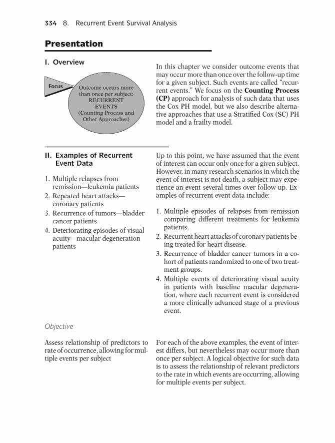
334 8. Recurrent Event Survival Analysis
Presentation
I. Overview
Outcome occurs morethan once per subject:
RECURRENTEVENTS
(Counting Process andOther Approaches)
Focus
In this chapter we consider outcome events thatmay occur more than once over the follow-up timefor a given subject. Such events are called “recur-rent events.” We focus on the Counting Process(CP) approach for analysis of such data that usesthe Cox PH model, but we also describe alterna-tive approaches that use a Stratified Cox (SC) PHmodel and a frailty model.
II. Examples of RecurrentEvent Data
Up to this point, we have assumed that the eventof interest can occur only once for a given subject.However, in many research scenarios in which theevent of interest is not death, a subject may expe-rience an event several times over follow-up. Ex-amples of recurrent event data include:
1. Multiple episodes of relapses from remissioncomparing different treatments for leukemiapatients.
2. Recurrent heart attacks of coronary patients be-ing treated for heart disease.
3. Recurrence of bladder cancer tumors in a co-hort of patients randomized to one of two treat-ment groups.
4. Multiple events of deteriorating visual acuityin patients with baseline macular degenera-tion, where each recurrent event is considereda more clinically advanced stage of a previousevent.
1. Multiple relapses fromremission—leukemia patients
2. Repeated heart attacks—coronary patients
3. Recurrence of tumors—bladdercancer patients
4. Deteriorating episodes of visualacuity—macular degenerationpatients
Objective
Assess relationship of predictors torate of occurrence, allowing for mul-tiple events per subject
For each of the above examples, the event of inter-est differs, but nevertheless may occur more thanonce per subject. A logical objective for such datais to assess the relationship of relevant predictorsto the rate in which events are occurring, allowingfor multiple events per subject.

Presentation: II. Examples of Recurrent Event Data 335
LEUKEMIA EXAMPLE
Do treatment groups differ in rates ofrelapse from remission?
In the leukemia example above, we might askwhether persons in one treatment group are ex-periencing relapse episodes at a higher rate thanpersons in a different treatment group.
Do smokers have a higher heart attack ratethan nonsmokers?
HEART ATTACK EXAMPLE If the recurrent event is a heart attack, we mightask, for example, whether smokers are experienc-ing heart attack episodes at a higher rate than non-smokers.
All events are of the same type
The order of events is not important
Heart attacks: Treat as identical events; Don't distinguish among 1st, 2nd, 3rd, etc. attack
LEUKEMIA AND HEART ATTACK EXAMPLES
For either of the above two examples, we are treat-ing all events as if they were the same type. That is,the occurrence of an event on a given subject iden-tifies the same disease without considering morespecific qualifiers such as severity or stage of dis-ease. We also are not taking into account the orderin which the events occurred.
For example, we may wish to treat all heart at-tacks, whether on the same or different subjects,as identical types of events, and we don’t wish toidentify whether a given heart attack episode wasthe first, or the second, or the third event that oc-curred on a given subject.
BLADDER CANCER EXAMPLE
Compare overall tumor recurrence ratewithout considering order or type of tumor
The third example, which considers recurrence ofbladder cancer tumors, can be considered simi-larly. That is, we may be interested in assessingthe “overall” tumor recurrence rate without dis-tinguishing either the order or type of tumor.
MACULAR DEGENERATION OFVISUAL ACUITY EXAMPLE
A second or higher event is more severethan its preceding event
Order of event is important
The fourth example, dealing with macular degen-eration events, however, differs from the other ex-amples. The recurrent events on the same subjectdiffer in that a second or higher event indicates amore severe degenerative condition than its pre-ceding event.
Consequently, the investigator in this scenariomay wish to do separate analyses for each orderedevent in addition to or instead of treating all recur-rent events as identical.

336 8. Recurrent Event Survival Analysis
Use a different analysis dependingon whether
a. recurrent events are treated asidentical
b. recurrent events involve differentdisease categories and/or theorder of events is important
We have thus made an important distinction tobe considered in the analysis of recurrent eventdata. If all recurrent events on the same subjectare treated as identical, then the analysis requiredof such data is different than what is required ifeither recurrent events involve different diseasecategories and/or the order that events reoccur isconsidered important.
Recurrent events identical⇓
Counting Process Approach(Andersen et al., 1993)
Recurrent events: different diseasecategories or event order important
⇓Stratified Cox (SC) ModelApproaches
The approach to analysis typically used when re-current events are treated as identical is calledthe Counting Process Approach (Andersen et al.,1993).
When recurrent events involve different diseasecategories and/or the order of events is consideredimportant, a number of alternative approaches toanalysis have been proposed that involve usingstratified Cox (SC) models.
In this chapter, we focus on the Counting Process(CP) approach, but also describe the other strati-fied Cox approaches (in a later section).
III. Counting Process Example To illustrate the counting process approach,we consider data on two hypothetical subjects(Table 8.1), Al and Hal, from a randomized trialthat compares two treatments for bladder cancertumors.
Al gets recurrent bladder cancer tumors at months3, 9, and 21, and is without a bladder cancer tumorat month 23, after which he is no longer followed.Al received the treatment coded as 1.
Hal gets recurrent bladder cancer tumors atmonths 3, 15, and 25, after which he is no longerfollowed. Hal received the treatment coded as 0.
Table 8.1. 2 Hypothetical SubjectsBladder Cancer Tumor Events
Time Event Treatmentinterval indicator group
Al 0 to 3 1 13 to 9 1 19 to 21 1 1
21 to 23 0 1
Hal 0 to 3 1 03 to 15 1 0
15 to 25 1 0

Presentation: III. Counting Process Example 337
Al Hal
No. recurrent 3 3events
Follow-up 23 months 25 monthstime
Event times 3, 9, 21 3, 15, 25from startof follow-up
Additional 2 months 0 monthsmonths offollow-upafter lastevent
Al has experienced 3 events of the same type(i.e., recurrent bladder tumors) over a follow-upperiod of 23 months. Hal has also experienced3 events of the same type over a follow-up periodof 25 months.
The 3 events experienced by Al occurred at differ-ent survival times (from the start of initial follow-up) from the 3 events experienced by Hal.
Also, Al had an additional 2 months of follow-upafter his last recurrent event during which timeno additional event occurred. In contrast, Hal hadno additional event-free follow-up time after hislast recurrent event.
Table 8.2. Example of Data Layoutfor Counting Process Approach
Interval Time Time Event TreatmentSubj Number Start Stop Status Group
Al 1 0 3 1 1Al 2 3 9 1 1Al 3 9 21 1 1Al 4 21 23 0 1Hal 1 0 3 1 0Hal 2 3 15 1 0Hal 3 15 25 1 0
Counting process: Start and Stoptimes
Standard layout: only Stop(survival) times (no recurrentevents)
In Table 8.2, we show for these 2 subjects, howthe data would be set up for computer analysesusing the counting process approach. Each sub-ject contributes a line of data for each time inter-val corresponding to each recurrent event and anyadditional event-free follow-up interval.
A distinguishing feature of the data layout for thecounting process approach is that each line of datafor a given subject lists the start time and stoptime for each interval of follow-up. This contrastswith the standard layout for data with no recurrentevents, which lists only the stop (survival) time.
Interval Time Time Event TreatmentSubj Number Start Stop Status Group
Sal 1 0 17 1 0Mal 1 0 12 0 1
Note that if a third subject, Sal, failed without fur-ther events or follow-up occurring, then Sal con-tributes only one line of data, as shown at the left.Similarly, only one line of data is contributed by a(fourth) subject, Mal, who was censored withouthaving failed at any time during follow-up.
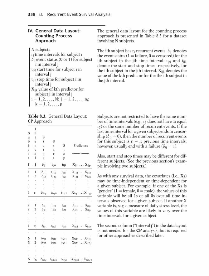
338 8. Recurrent Event Survival Analysis
IV. General Data Layout:Counting ProcessApproach
The general data layout for the counting processapproach is presented in Table 8.3 for a datasetinvolving N subjects.
The ith subject has ri recurrent events. δij denotesthe event status (1 = failure, 0 = censored) for theith subject in the jth time interval. tij0 and tij1denote the start and stop times, respectively, forthe ith subject in the jth interval. Xijk denotes thevalue of the kth predictor for the the ith subject inthe jth interval.
⎧⎪⎪⎪⎪⎪⎪⎪⎪⎪⎪⎪⎪⎪⎪⎪⎪⎪⎨⎪⎪⎪⎪⎪⎪⎪⎪⎪⎪⎪⎪⎪⎪⎪⎪⎪⎩
N subjectsri time intervals for subject iδij event status (0 or 1) for subject
i in interval jtij0 start time for subject i in
interval jtij1 stop time for subject i in
interval jXijk value of kth predictor for
subject i in interval ji = 1, 2, . . . , N; j = 1, 2, . . . , ni;
k = 1, 2, . . . , p
Table 8.3. General Data Layout:CP Approach
IS nu t Sb e t Sj r a t S Predictorse v t a tc a u r o ︷ ︸︸ ︷t l s t p
i j δij tij0 tij1 Xij1 . . . Xijp
1 1 δ11 t110 t111 X111 . . . X11p
1 2 δ12 t120 t121 X121 . . . X12p
· · · · · · ·· · · · · · ·· · · · · · ·1 r1 δ1r1 t1r10 t1r11 X1r11 . . . X1r1p
· · · · · · ·i 1 δi1 ti10 ti11 Xi11 . . . Xi1p
i 2 δi2 ti20 ti21 Xi21 . . . Xi2p
· · · · · · ·· · · · · · ·· · · · · · ·i ri δiri tiri0 tiri1 Xiri1 . . . Xirip
· · · · · · ·N 1 δN1 tN10 tN11 XN11 . . . XN1p
N 2 δN2 tN20 tN21 XN21 . . . XN2p
· · · · · · ·· · · · · · ·· · · · · · ·N rN δNrN tNrN0 tNrN1 XNrN1 . . .XNrNp
Subjects are not restricted to have the same num-ber of time intervals (e.g., r1 does not have to equalr2) or the same number of recurrent events. If thelast time interval for a given subject ends in censor-ship (δij = 0), then the number of recurrent eventsfor this subject is ri − 1; previous time intervals,however, usually end with a failure (δij = 1).
Also, start and stop times may be different for dif-ferent subjects. (See the previous section’s exam-ple involving two subjects.)
As with any survival data, the covariates (i.e., Xs)may be time-independent or time-dependent fora given subject. For example, if one of the Xs is“gender” (1 = female, 0 = male), the values of thisvariable will be all 1s or all 0s over all time in-tervals observed for a given subject. If another Xvariable is, say, a measure of daily stress level, thevalues of this variable are likely to vary over thetime intervals for a given subject.
The second column (“Interval j”) in the data layoutis not needed for the CP analysis, but is requiredfor other approaches described later.
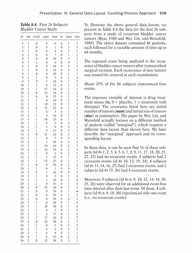
Presentation: IV. General Data Layout: Counting Process Approach 339
Table 8.4. First 26 Subjects:Bladder Cancer Study
id int event start stop tx num size
1 1 0 0 0 0 1 12 1 0 0 1 0 1 33 1 0 0 4 0 2 14 1 0 0 7 0 1 15 1 0 0 10 0 5 16 1 1 0 6 0 4 16 2 0 6 10 0 4 17 1 0 0 14 0 1 18 1 0 0 18 0 1 19 1 1 0 5 0 1 39 2 0 5 18 0 1 3
10 1 1 0 12 0 1 110 2 1 12 16 0 1 110 3 0 16 18 0 1 111 1 0 0 23 0 3 312 1 1 0 10 0 1 312 2 1 10 15 0 1 312 3 0 15 23 0 1 313 1 1 0 3 0 1 113 2 1 3 16 0 1 113 3 1 16 23 0 1 114 1 1 0 3 0 3 114 2 1 3 9 0 3 114 3 1 9 21 0 3 114 4 0 21 23 0 3 115 1 1 0 7 0 2 315 2 1 7 10 0 2 315 3 1 10 16 0 2 315 4 1 16 24 0 2 316 1 1 0 3 0 1 116 2 1 3 15 0 1 116 3 1 15 25 0 1 117 1 0 0 26 0 1 218 1 1 0 1 0 8 118 2 0 1 26 0 8 119 1 1 0 2 0 1 419 2 1 2 26 0 1 420 1 1 0 25 0 1 220 2 0 25 28 0 1 221 1 0 0 29 0 1 422 1 0 0 29 0 1 223 1 0 0 29 0 4 124 1 1 0 28 0 1 624 2 1 28 30 0 1 625 1 1 0 2 0 1 525 2 1 2 17 0 1 525 3 1 17 22 0 1 525 4 0 22 30 0 1 526 1 1 0 3 0 2 126 2 1 3 6 0 2 126 3 1 6 8 0 2 126 4 1 8 12 0 2 126 5 0 12 30 0 2 1
To illustrate the above general data layout, wepresent in Table 8.4 the data for the first 26 sub-jects from a study of recurrent bladder cancertumors (Byar, 1980 and Wei, Lin, and Weissfeld,1989). The entire dataset contained 86 patients,each followed for a variable amount of time up to64 months.
The repeated event being analyzed is the recur-rence of bladder cancer tumors after transurethralsurgical excision. Each recurrence of new tumorswas treated by removal at each examination.
About 25% of the 86 subjects experienced fourevents.
The exposure variable of interest is drug treat-ment status (tx, 0 = placebo, 1 = treatment withthiotepa). The covariates listed here are initialnumber of tumors (num) and initial size of tumors(size) in centimeters. The paper by Wei, Lin, andWeissfeld actually focuses on a different methodof analysis (called “marginal”), which requires adifferent data layout than shown here. We laterdescribe the “marginal” approach and its corre-sponding layout.
In these data, it can be seen that 16 of these sub-jects (id #s 1, 2, 3, 4, 5, 6, 7, 8, 9, 11, 17, 18, 20, 21,22, 23) had no recurrent events, 4 subjects had 2recurrent events (id #s 10, 12, 19, 24), 4 subjects(id #s 13, 14, 16, 25) had 3 recurrent events, and 2subjects (id #s 15, 26) had 4 recurrent events.
Moreover, 9 subjects (id #s 6, 9, 10, 12, 14, 18, 20,25, 26) were observed for an additional event-freetime interval after their last event. Of these, 4 sub-jects (id #s 6, 9, 18, 20) experienced only one event(i.e., no recurrent events).

340 8. Recurrent Event Survival Analysis
V. The Counting ProcessModel and Method
The model typically used to carry out the Count-ing Process approach is the standard Cox PHmodel, once again shown here at the left.
As usual, the PH assumption needs to be evalu-ated for any time-independent variable. A strati-fied Cox model or an extended Cox model wouldneed to be used if one or more time-independentvariables did not satisfy the PH assumption. Also,an extended Cox model would be required if inher-ently time-dependent variables were considered.
Cox PH Model
h(t, X) = h0(t) exp[�βiXi]
Need to
Assess PH assumption for Xi
Consider stratified Cox or extendedCox if PH assumption notsatisfied
Use extended Cox for time-dependent variables
The primary difference in the way the Cox modelis used for analyzing recurrent event data versusnonrecurrent (one time interval per subject) datais the way several time intervals on the same sub-ject are treated in the formation of the likelihoodfunction maximized for the Cox model used.
To keep things simple, we assume that the datainvolve only time-independent variables satisfyingthe PH assumption. For recurrent survival data, asubject with more than one time interval remainsin the risk set until his or her last interval, afterwhich the subject is removed from the risk set. Incontrast, for nonrecurrent event data, each subjectis removed from the risk set at the time of failureor censorship.
Nevertheless, for subjects with two or more in-tervals, the different lines of data contributed bythe same subject are treated in the analysis as ifthey were independent contributions from differ-ent subjects, even though there are several out-comes on the same subject.
In contrast, for the standard Cox PH model ap-proach for nonrecurrent survival data, differentlines of data are treated as independent becausethey come from different subjects.
Recurrent event Nonrecurrentdata event data(Likelihood function formed differently)
Subjects with >1time intervalremain in the riskset until lastinterval iscompleted
Subjects removedfrom risk set attime of failureor censorship
Different lines ofdata are treatedas independenteven thoughseveral outcomeson the samesubject
Different lines ofdata are treatedas independentbecause theycome fromdifferentsubjects

Presentation: V. The Counting Process Model and Method 341
Cox PH Model for CP Approach:Bladder Cancer Study
For the bladder cancer study described inTable 8.4, the basic Cox PH model fit to these datatakes the form shown at the left.
h(t, X) = h0(t)exp[β tx + γ1 num+γ2 size]
where
tx = 1 if thiotepa, 0 if placebonum = initial # of tumorssize = initial size of tumors
The primary (exposure) variable of interest in thismodel is the treatment variable tx. The variablesnum and size are considered as potential con-founders. All three variables are time-independentvariables.
No-interaction Model This is a no-interaction model because it does notcontain product terms of the form tx × num ortx × size. An interaction model involving suchproduct terms could also be considered, but weonly present the no-interaction model for illustra-tive purposes.
Interaction model would involveproduct terms
tx × num and/or tx × size
Table 8.5. Ordered Failure Timeand Risk Set Information for First26 Subjects in Bladder CancerStudy
SubjectOrdered # in # ID #s forfailure risk # censored outcomestimes set failed in int(j) nj mj [t(j), t(j+1)) [t(j), t(j+1))
0 26 — 1 11 25 1 1 2, 182 24 2 0 19, 253 24 4 1 3, 13, 14,
16, 265 23 1 0 96 23 2 0 6, 267 23 1 1 4, 158 22 1 0 269 22 1 0 14
10 22 2 2 5, 6, 12, 1512 20 2 1 7, 10, 2615 19 2 0 12, 1616 19 3 0 10, 13, 1517 19 1 3 8, 9, 10, 2521 16 1 0 1422 16 1 0 2523 16 1 3 11, 12, 13, 1424 12 1 0 1525 11 2 0 16, 2026 10 1 2 17, 18, 1928 7 1 4 20, 21, 22,
23, 2430 3 1 2 24, 25, 26
32 21
Table 8.5 at the left provides ordered failure timesand corresponding risk set information that wouldresult if the first 26 subjects that we described inTable 8.4 comprised the entire dataset. (Recall thatthere are 86 subjects in the complete dataset.)
Because we consider 26 subjects, the number inthe risk set at ordered failure time t(0) is n(0) = 26.As these subjects fail (i.e., develop a bladder cancertumor) or are censored over follow-up, the num-ber in the risk set will decrease from the jth tothe j + 1th ordered failure time provided that nosubject who fails at time t(j) either has a recurrentevent at a later time or has additional follow-uptime until later censorship. In other words, a sub-ject who has additional follow-up time after havingfailed at t( j ) does not drop out of the risk set aftert( j ).

342 8. Recurrent Event Survival Analysis
Table 8.6. Focus on Subject #s 19and 25
t(j) nj mj q(j) Subject ID #s
0 26 — 1 11 25 1 1 2, 182 24 2 0 19, 253 24 4 1 3, 13, 14, 16, 26
•••
17 19 1 3 8, 9, 10, 2521 16 1 0 1422 16 1 0 2523 16 1 3 11, 12, 13, 1424 12 1 0 1525 11 2 0 16, 2026 10 1 2 17, 18, 1928 7 1 4 20, 21, 22, 23, 2430 3 1 2 24, 25, 26
For example, at month t(j) = 2, subject #s 19 and25 fail, but the number in the risk set at that time(nj = 24) does not decrease (by 2) going into thenext failure time because each of these subjectshas later recurrent events. In particular, subject#19 has a recurrent event at month t(j) = 26 andsubject #25 has two recurrent events at monthst(j) = 17 and t(j) = 22 and has additional follow-up time until censored month 30.
Table 8.7. Focus on Subject #s 3,13, 14, 16, 26
t(j) nj mj q(j) Subject ID #s
0 26 — 1 11 25 1 1 2, 182 24 2 0 19, 253 24 4 1 3, 13, 14, 16, 265 23 1 0 96 23 2 0 6, 267 23 1 1 4, 158 22 1 0 269 22 1 0 14
10 22 2 2 5, 6, 12, 1512 20 2 1 7, 10, 2615 19 2 0 12, 1616 19 3 0 10, 13, 1517 19 1 3 8, 9, 10, 2521 16 1 0 1422 16 1 0 2523 16 1 3 11, 12, 13, 1424 12 1 0 1525 11 2 0 16, 2026 10 1 2 17, 18, 1928 7 1 4 20, 21, 22, 23, 2430 3 1 2 24, 25, 26
As another example from Table 8.5, subject #s 3,13, 14, 16, 26 contribute information at orderedfailure time t(j) = 3, but the number in the risk setonly drops from 24 to 23 even though the last fourof these subjects all fail at t(j) = 3. Subject #3 iscensored at month 4 (see Table 8.4), so this sub-ject is removed from the risk set after failure timet(j) = 3. However, subjects 13, 14, 16, and 26 allhave recurrent events after t(j) = 3, so they are notremoved from the risk set after t(j) = 3.
Subject #26 appears in the last column 5 times.This subject contributes 5 (start, stop) time inter-vals, fails at months 3, 6, 8, and 12, and is alsofollowed until month 30, when he is censored.

Presentation: V. The Counting Process Model and Method 343
“Gaps” in follow-up time:
0 10 25 50gaplost re-enter
Another situation, which is not illustrated in thesedata, involves “gaps” in a subject’s follow-up time.A subject may leave the risk set (e.g., lost to follow-up) at, say, time = 10 and then re-enter the riskset again and be followed from, say, time = 25 totime = 50. This subject has a follow-up gap duringthe period from time = 10 to time = 25.No Interaction Cox PH Model
The (partial) likelihood function (L) used to fit theno-interaction Cox PH model is expressed in typi-cal fashion as the product of individual likelihoodscontributed by each ordered failure time and cor-responding risk set information in Table 8.5. Thereare 22 such terms in this product because there are22 ordered failure times listed in Table 8.5.
h(t,X) = h0(t)exp[β tx + γ1 num+γ2 size]
Partial likelihood function:
L = L1 × L2 × · · · × L22
Lj = individual likelihood at t(j)
= Pr[failing at t(j) | survival up tot(j)]
j = 1, 2, . . . , 22
Lj = exp (βtx(j) + γ1num(j) + γ2size(j))∑s in R(t(j) )
exp (βtxs(j) +γ1nums(j) +γ2sizes(j))
Each individual likelihood Lj essentially gives theconditional probability of failing at time t(j), givensurvival (i.e., remaining in the risk set) at t(j).
If there is only one failure at the jth ordered fail-ure time, Lj is expressed as shown at the left forthe above no-interaction model. In this expressiontx(j), num(j), and size(j) denote the values of thevariables tx, num, and size for the subject failingat month t(j).
tx(j), num(j), and size(j) values of tx,num, and size at t(j)
txs(j), nums(j), and sizes(j) values of tx,num, and size for subject s in R(t(j))
The terms txs(j), nums(j), and sizes(j) denote the val-ues of the variables tx, num, and size for the sub-ject s in the risk set R(t(j)). Recall that R(t(j)) con-sists of all subjects remaining at risk at failuretime t(j).
Data for Subject #25
id int event start stop tx num size
25 1 1 0 2 0 1 525 2 1 2 17 0 1 525 3 1 17 22 0 1 525 4 0 22 30 0 1 5
j = 15th ordered failure timen15 = 16 subjects in risk set att(15) = 22:
R(t(15) = 22) = {subject #s 11, 12,13, 14, 15, 16, 17, 18, 19, 20, 21,22, 23, 24, 25, 26}
For example, subject #25 from Table 8.4 failed forthe third time at month 22, which is the j = 15thordered failure time listed in Table 8.5. It can beseen that nj = 16 of the initial 26 subjects are stillat risk at the beginning of month 22. The risk setat this time includes subject #25 and several othersubjects (#s 12, 13, 14, 15, 16, 18, 19, 26) who al-ready had at least one failure prior to month 22.

344 8. Recurrent Event Survival Analysis
L15 = exp(β(0) + γ1(1) + γ1(5))∑s in R(t(15) )
exp(βtxs(15) + γ1nums(15) + γ1sizes(15))The corresponding likelihood L15 at t(15) = 22 isshown at the left. Subject #25’s values tx25(15) = 0,num25(15) = 1, and size25(15) = 5, have been in-serted into the numerator of the formula. The de-nominator will contain a sum of 16 terms, one foreach subject in the risk set at t(15) = 22.
Computer program formulatespartial likelihood L(See Computer Appendix)
The overall partial likelihood L will be formulatedinternally by the computer program once the datalayout is in the correct form and the program codeused involves the (start, stop) formulation.
VI. Robust Estimation As illustrated for subject #14 at the left, each sub-ject contributes a line of data for each time inter-val corresponding to each recurrent event and anyadditional event-free follow-up interval.
Data for Subject #14
id int event start stop tx num size
14 1 1 0 3 0 3 114 2 1 3 9 0 3 114 3 1 9 21 0 3 114 4 0 21 23 0 3 1
Up to this point:the 4 lines of data for subject #14 aretreated as independent observations
We have also pointed out that the Cox model anal-ysis described up to this point treats differentlines of data contributed by the same subject asif they were independent contributions from dif-ferent subjects.
Nevertheless,
� Observations of the samesubject are correlated� Makes sense to adjust for suchcorrelation in the analysis
Nevertheless, it makes sense to view the differentintervals contributed by a given subject as repre-senting correlated observations on the same sub-ject that must be accounted for in the analysis.
Robust (Empirical) Estimation A widely used technique for adjusting for the cor-relation among outcomes on the same subject iscalled robust estimation (also referred to as em-pirical estimation). This technique essentially in-volves adjusting the estimated variances of re-gression coefficients obtained for a fitted modelto account for misspecification of the correlationstructure assumed (see Zeger and Liang, 1986 andKleinbaum and Klein, 2002).
� Adjusts
Var (βk)
where
βk
is an estimated regressioncoefficient� accounts for misspecification ofassumed correlation structure

Presentation: VI. Robust Estimation 345
CP approach: assumesindependence
Goal of robust estimation: adjust forcorrelation within subjects
In the CP approach, the assumed correlationstructure is independence; that is, the Cox PHmodel that is fit assumes that different outcomeson the same subject are independent. Thereforethe goal of robust estimation for the CP approachis to obtain variance estimators that adjust for cor-relation within subjects when previously no suchcorrelation was assumed.
Same goal for other approaches foranalyzing recurrent event data
This is the same goal for other approaches for an-alyzing recurrent event data that we describe laterin this chapter.
Do not adjust
βk
Only adjust
Var (βk)
Note that the estimated regression coefficientsthemselves are not adjusted; only the estimatedvariances of these coefficients are adjusted.
Robust (Empirical) Variance The robust (i.e., empirical) estimator of the vari-ance of an estimated regression coefficient there-fore allows tests of hypotheses and confidence in-tervals about model parameters that account forcorrelation within subjects.
allowstests of hypotheses andconfidence intervals
that account for correlated data
Matrix formula:
derived from ML estimation
We briefly describe the formula for the robust vari-ance estimator below. This formula is in matrixform and involves terms that derive from the setof “score” equations that are used to solve for MLestimates of the regression coefficients. This in-formation may be of interest to the more mathe-matically inclined reader with some backgroundin methods for the analysis of correlated data(Kleinbaum and Klein, 2002).
Formula not essential for usingcomputer packages
However, the information below is not essentialfor an understanding of how to obtain robust esti-mators using computer packages. (See ComputerAppendix for the code using SAS and Stata.)
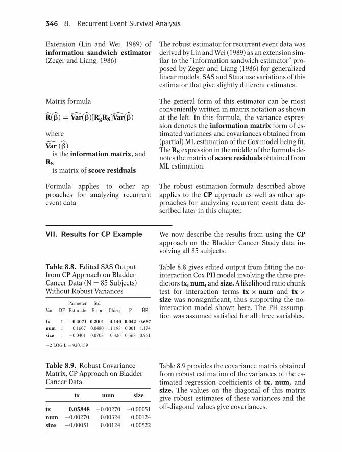
346 8. Recurrent Event Survival Analysis
Extension (Lin and Wei, 1989) ofinformation sandwich estimator(Zeger and Liang, 1986)
The robust estimator for recurrent event data wasderived by Lin and Wei (1989) as an extension sim-ilar to the “information sandwich estimator” pro-posed by Zeger and Liang (1986) for generalizedlinear models. SAS and Stata use variations of thisestimator that give slightly different estimates.
Matrix formula
R(β) = Var(β)[R′SRS]Var(β)
where
Var (β)is the information matrix, and
RSis matrix of score residuals
The general form of this estimator can be mostconveniently written in matrix notation as shownat the left. In this formula, the variance expres-sion denotes the information matrix form of es-timated variances and covariances obtained from(partial) ML estimation of the Cox model being fit.The RS expression in the middle of the formula de-notes the matrix of score residuals obtained fromML estimation.
Formula applies to other ap-proaches for analyzing recurrentevent data
The robust estimation formula described aboveapplies to the CP approach as well as other ap-proaches for analyzing recurrent event data de-scribed later in this chapter.
VII. Results for CP Example We now describe the results from using the CPapproach on the Bladder Cancer Study data in-volving all 85 subjects.
Table 8.8. Edited SAS Outputfrom CP Approach on BladderCancer Data (N = 85 Subjects)Without Robust Variances
Parmeter StdVar DF Estimate Error Chisq P HR
tx 1 −0.4071 0.2001 4.140 0.042 0.667num 1 0.1607 0.0480 11.198 0.001 1.174size 1 −0.0401 0.0703 0.326 0.568 0.961
−2 LOG L = 920.159
Table 8.8 gives edited output from fitting the no-interaction Cox PH model involving the three pre-dictors tx, num, and size. A likelihood ratio chunktest for interaction terms tx × num and tx ×size was nonsignificant, thus supporting the no-interaction model shown here. The PH assump-tion was assumed satisfied for all three variables.
Table 8.9. Robust CovarianceMatrix, CP Approach on BladderCancer Data
tx num size
tx 0.05848 −0.00270 −0.00051num −0.00270 0.00324 0.00124size −0.00051 0.00124 0.00522
Table 8.9 provides the covariance matrix obtainedfrom robust estimation of the variances of the es-timated regression coefficients of tx, num, andsize. The values on the diagonal of this matrixgive robust estimates of these variances and theoff-diagonal values give covariances.

Presentation: VIII. Other Approaches—Stratified Cox 347
Robust standard error for tx= square-root (.05848) = 0.2418
Nonrobust standard error for tx= 0.2001
Because the exposure variable of interest in thisstudy is tx, the most important value in this ma-trix is 0.05848. The square root of this value is0.2418, which gives the robust standard error ofthe estimated coefficient of the tx variable. Noticethat this robust estimator is similar but somewhatdifferent from the nonrobust estimator of 0.2001shown in Table 8.8.
Summary of Results fromCP Approach
We now summarize the CP results for the effectof the exposure variable tx on recurrent event sur-vival controlling for num and size. The hazard ra-tio estimate of .667 indicates that the hazard forthe placebo is 1.5 times the hazard for the treat-ment.
Hazard Ratio tx : exp(−0.407) = 0.667(= 1/1.5)
Wald Chi-Square tx : robust nonrobust2.83 4.14
P-value tx : .09 .04
(H0: no effect of tx, HA: two sided)
95% CI for HR tx (robust): (0.414,1.069)
HA: one-sided, both p-values < .05
We return to the analysis of thesedata when we discuss other ap-proaches for analysis of recurrentevent data.
Using robust estimation, the Wald statistic for thishazard ratio is borderline nonsignificant (P = .09).Using the nonrobust estimator, the Wald statisticis borderline significant (P = .04). Both these P-values, however, are for a two-sided alternative.For a one-sided alternative, both P-values wouldbe significant at the .05 level. The 95% confidenceinterval using the robust variance estimator isquite wide in any case.
VIII. Other Approaches—Stratified Cox
We now describe three other approaches for ana-lyzing recurrent event data, each of which uses aStratified Cox (SC) PH model. They are called con-ditional 1, conditional 2, and marginal. Theseapproaches are often used to distinguish the or-der in which recurrent events occur.
The “strata” variable for each approach treats thetime interval number as a categorical variable.
3 stratified Cox (SC) approaches:
Conditional 1 (Prentice,Williams and
Conditional 2 Peterson,1981)Marginal (Wei, Lin, and
Weissfeld,1989)
Goal: distinguish order of recurrentevents
Strata variable: time interval #treated ascategorical
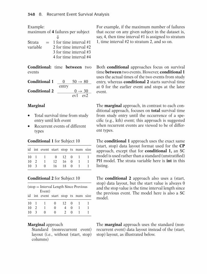
348 8. Recurrent Event Survival Analysis
Example:maximum of 4 failures per subject
⇓Strata = 1 for time interval #1variable 2 for time interval #2
3 for time interval #34 for time interval #4
For example, if the maximum number of failuresthat occur on any given subject in the dataset is,say, 4, then time interval #1 is assigned to stratum1, time interval #2 to stratum 2, and so on.
Conditional: time between twoevents
Conditional 1 0 50 → 80entry
Conditional 2 0 → 30ev1 ev2
Both conditional approaches focus on survivaltime between two events. However, conditional 1uses the actual times of the two events from studyentry, whereas conditional 2 starts survival timeat 0 for the earlier event and stops at the laterevent.
Marginal
� Total survival time from studyentry until kth event� Recurrent events of differenttypes
The marginal approach, in contrast to each con-ditional approach, focuses on total survival timefrom study entry until the occurrence of a spe-cific (e.g., kth) event; this approach is suggestedwhen recurrent events are viewed to be of differ-ent types.
Conditional 1 for Subject 10
id int event start stop tx num size
10 1 1 0 12 0 1 110 2 1 12 16 0 1 110 3 0 16 18 0 1 1
The conditional 1 approach uses the exact same(start, stop) data layout format used for the CPapproach, except that for conditional 1, an SCmodel is used rather than a standard (unstratified)PH model. The strata variable here is int in thislisting.
Conditional 2 for Subject 10
(stop = Interval Length Since PreviousEvent)
id int event start stop tx num size
10 1 1 0 12 0 1 110 2 1 0 4 0 1 110 3 0 0 2 0 1 1
The conditional 2 approach also uses a (start,stop) data layout, but the start value is always 0and the stop value is the time interval length sincethe previous event. The model here is also a SCmodel.
Marginal approachStandard (nonrecurrent event)layout (i.e., without (start, stop)columns)
The marginal approach uses the standard (non-recurrent event) data layout instead of the (start,stop) layout, as illustrated below.

Presentation: VIII. Other Approaches—Stratified Cox 349
Marginal Approach for Subject 10
id int event stime tx num size
10 1 1 12 0 1 110 2 1 16 0 1 110 3 0 18 0 1 110 4 0 18 0 1 1
The marginal approach layout, shown at the left,contains four lines of data in contrast to the threelines of data that would appear for subject #10using the CP, conditional 1, and conditional 2approaches
Marginal approachEach subject at risk for all failuresthat might occur
# actual failures ≤ # possible failures
The reason why there are 4 lines of data here isthat, for the marginal approach, each subject isconsidered to be at risk for all failures that mightoccur, regardless of the number of events a subjectactually experienced.
Bladder cancer data:
Maximum # (possible) failures = 4
So, subject 10 (as well as all othersubjects) gets 4 lines of data
Because the maximum number of failures be-ing considered in the bladder cancer data is 4(e.g., for subject #s 15 and 26), subject #10, whofailed only twice, will have two additional linesof data corresponding to the two additional fail-ures that could have possibly occurred for thissubject.
Fundamental Difference Amongthe 3 SC Approaches
The three alternative SC approaches (conditional1, conditional 2, and marginal) fundamentallydiffer in the way the risk set is determined forstrata corresponding to events after the first event.Risk set differs for strata after first
event
Conditional 2: time until 1st eventdoes not influence risk set for laterevents (i.e., clock reset to 0 afterevent occurs)
With conditional 2, the time until the first eventdoes not influence the composition of the risk setfor a second or later event. In other words, theclock for determining who is at risk gets reset to 0after each event occurs.
Conditional 1: time until 1st eventinfluences risk set for later events
In contrast, with conditional 1, the time until thefirst event affects the composition of the risk setfor later events.
Marginal: risk set determined fromtime since study entry
With the marginal approach, the risk set for thekth event (k = 1, 2, . . .) identifies those at risk forthe kth event since entry into the study.
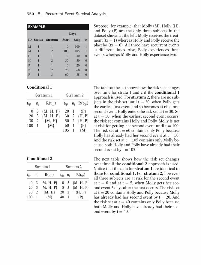
350 8. Recurrent Event Survival Analysis
EXAMPLE
Days
ID Status Stratum Start Stop tx
M 1 11M 2 11
H 1 01
H 2 01
P 1 01
P 2 01P 3
0100
0
30
0
2060
100105
30
50
20
6085 01
Suppose, for example, that Molly (M), Holly (H),and Polly (P) are the only three subjects in thedataset shown at the left. Molly receives the treat-ment (tx = 1) whereas Holly and Polly receive theplacebo (tx = 0). All three have recurrent eventsat different times. Also, Polly experiences threeevents whereas Molly and Holly experience two.
Conditional 1
Stratum 1 Stratum 2
t(j) nj R(t(j)) t(j) nj R(t(j))
0 3 {M, H, P} 20 1 {P}20 3 {M, H, P} 30 2 {H, P}30 2 {M, H} 50 2 {H, P}
100 1 {M} 60 1 {P}105 1 {M}
The table at the left shows how the risk set changesover time for strata 1 and 2 if the conditional 1approach is used. For stratum 2, there are no sub-jects in the risk set until t = 20, when Polly getsthe earliest first event and so becomes at risk for asecond event. Holly enters the risk set at t = 30. Soat t = 50, when the earliest second event occurs,the risk set contains Holly and Polly. Molly is notat risk for getting her second event until t = 100.The risk set at t = 60 contains only Polly becauseHolly has already had her second event at t = 50.And the risk set at t = 105 contains only Molly be-cause both Holly and Polly have already had theirsecond event by t = 105.
Conditional 2
Stratum 1 Stratum 2
t(j) nj R(t(j)) t(j) nj R(t(j))
0 3 {M, H, P} 0 3 {M, H, P}20 3 {M, H, P} 5 3 {M, H, P}30 2 {M, H} 20 2 {H, P}
100 1 {M} 40 1 {P}
The next table shows how the risk set changesover time if the conditional 2 approach is used.Notice that the data for stratum 1 are identical tothose for conditional 1. For stratum 2, however,all three subjects are at risk for the second eventat t = 0 and at t = 5, when Molly gets her sec-ond event 5 days after the first occurs. The risk setat t = 20 contains Holly and Polly because Mollyhas already had her second event by t = 20. Andthe risk set at t = 40 contains only Polly becauseboth Molly and Holly have already had their sec-ond event by t = 40.

Presentation: VIII. Other Approaches—Stratified Cox 351
Marginal
Stratum 1 Stratum 2
t(j) nj R(t(j)) t(j) nj R(t(j))
0 3 {M, H, P} 0 3 {M, H, P}20 3 {M, H, P} 50 3 {M, H, P}30 2 {M, H} 60 2 {M, P}
100 3 {M} 105 1 {M}
We next consider the marginal approach. Forstratum 1, the data are identical again to those forconditional 1. For stratum 2, however, all threesubjects are at risk for the second event at t = 0and at t = 50, when Holly gets her second event.The risk set at t = 60 contains Molly and Polly be-cause Holly has already had her second event att = 50. And the risk set at t = 105 contains onlyMolly because both Holly and Polly have alreadyhad their second event by t = 60.
Stratum 3 for Marginal approachfollows
Because Polly experienced three events, there isalso a third stratum for this example, which wedescribe for the marginal approach only.
MarginalStratum 3
t(j) nj R(t(j))
0 3 {M, H, P}85 2 {M, P}Note: H censored by t = 85
Using the marginal approach, all three subjects areconsidered at risk for the third event when theyenter the study (t = 0), even though Molly andHolly actually experience only two events. At t =85, when Polly has her third event, Holly, whosefollow-up ended at t = 50, is no longer in therisk set; which still includes Molly because Molly’sfollow-up continues until t = 105.
Basic idea (marginal approach):
Each failure considered aseparate process
Allows stratifying on
� Failure order� Different failure type(e.g., stage 1 vs. stage 2 cancer)
The basic idea behind the marginal approach isthat it allows each failure to be considered as aseparate process. Consequently, the marginal ap-proach not only allows the investigator to considerthe ordering of failures as separate events (i.e.,strata) of interest, but also allows the different fail-ures to represent different types of events that mayoccur on the same subject.
Stratified Cox PH (SC) Model for all3 alternative approaches
Use standard computer program forSC (e.g., SAS’s PHREG, Stata’s stcox,SPSS’s coxreg)
All three alternative approaches, although differ-ing in the form of data layout and the way the riskset is determined, nevertheless use a stratified CoxPH model to carry out the analysis. This allows astandard program that fits a SC model (e.g., SAS’sPHREG) to perform the analysis.
No-interaction SC model for blad-der cancer data
hg(t,X) = h0g(t)exp[β tx + γ1 num+γ2 size]
where g = 1, 2, 3, 4
The models used for the three alternative SC ap-proaches are therefore of the same form. For ex-ample, we show on the left the no-interaction SCmodel appropriate for the bladder cancer data wehave been illustrating.

352 8. Recurrent Event Survival Analysis
Two types of SC models:
No-interaction versus interactionmodel
Typically compared using LR test
As described previously in Chapter 5 on the strati-fied Cox procedure, a no-interaction stratified Coxmodel is not appropriate if there is interactionbetween the stratified variables and the predictorvariables put into the model. Thus, it is necessaryto assess whether an interaction version of the SCmodel is more appropriate, as typically carried outusing a likelihood ratio test.
Version 1: Interaction SC Model For the bladder cancer data, we show at theleft two equivalent versions of the SC interactionmodel. The first version separates the data into 4separate models, one for each stratum.
hg(t,X) = h0g(t)exp[βg tx
+γ1g num + γ2g size]
g = 1, 2, 3, 4
Version 2: Interaction SC Model The second version contains product terms involv-ing the stratified variable with each of the 3 pre-dictors in the model. Because there are 4 strata,the stratified variable is defined using 3 dummyvariables Z∗
1, Z∗2, and Z∗
3.
hg(t,X) = h0g(t)exp[β tx + γ1 num+γ2 size + δ11(Z∗
1 × tx)+ δ12(Z∗
2 × tx) + δ13(Z∗3 × tx)
+ δ21(Z∗1 × num) + δ22(Z∗
2 × num)+ δ23(Z∗
3 × num) + δ31(Z∗1 × size)
+ δ32(Z∗2 × size) + δ33(Z∗
3 × size)]
where Z∗1, Z∗
2, and Z∗3 are 3 dummy
variables for the 4 strata.
H0(Version 1) The null hypotheses for the LR test that comparesthe interaction with the no-interaction SC modelis shown at the left for each version. The df for theLR test is 9.
β1 = β2 = β3 = β4 ≡ β,
γ11 = γ12 = γ13 = γ14 ≡ γ1,
γ21 = γ22 = γ23 = γ24 ≡ γ2
H0(Version 2)
δ11 = δ12 = δ13 = δ21 = δ22 = δ23
= δ31 = δ32 = δ33 = 0
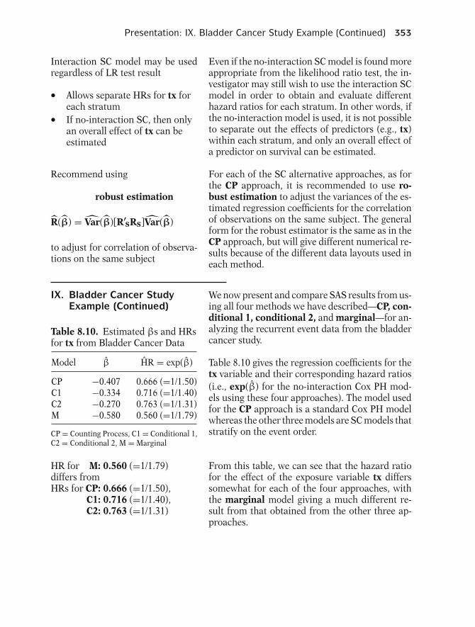
Presentation: IX. Bladder Cancer Study Example (Continued) 353
Interaction SC model may be usedregardless of LR test result
� Allows separate HRs for tx foreach stratum� If no-interaction SC, then onlyan overall effect of tx can beestimated
Even if the no-interaction SC model is found moreappropriate from the likelihood ratio test, the in-vestigator may still wish to use the interaction SCmodel in order to obtain and evaluate differenthazard ratios for each stratum. In other words, ifthe no-interaction model is used, it is not possibleto separate out the effects of predictors (e.g., tx)within each stratum, and only an overall effect ofa predictor on survival can be estimated.
Recommend using
robust estimation
R(β) = Var(β)[R′SRS]Var(β)
to adjust for correlation of observa-tions on the same subject
For each of the SC alternative approaches, as forthe CP approach, it is recommended to use ro-bust estimation to adjust the variances of the es-timated regression coefficients for the correlationof observations on the same subject. The generalform for the robust estimator is the same as in theCP approach, but will give different numerical re-sults because of the different data layouts used ineach method.
IX. Bladder Cancer StudyExample (Continued)
We now present and compare SAS results from us-ing all four methods we have described—CP, con-ditional 1, conditional 2, and marginal—for an-alyzing the recurrent event data from the bladdercancer study.
Table 8.10 gives the regression coefficients for thetx variable and their corresponding hazard ratios(i.e., exp(β) for the no-interaction Cox PH mod-els using these four approaches). The model usedfor the CP approach is a standard Cox PH modelwhereas the other three models are SC models thatstratify on the event order.
Table 8.10. Estimated βs and HRsfor tx from Bladder Cancer Data
Model β HR = exp(β)
CP −0.407 0.666 (=1/1.50)C1 −0.334 0.716 (=1/1.40)C2 −0.270 0.763 (=1/1.31)M −0.580 0.560 (=1/1.79)
CP = Counting Process, C1 = Conditional 1,C2 = Conditional 2, M = Marginal
HR for M: 0.560 (=1/1.79)differs fromHRs for CP: 0.666 (=1/1.50),
C1: 0.716 (=1/1.40),C2: 0.763 (=1/1.31)
From this table, we can see that the hazard ratiofor the effect of the exposure variable tx differssomewhat for each of the four approaches, withthe marginal model giving a much different re-sult from that obtained from the other three ap-proaches.

354 8. Recurrent Event Survival Analysis
Table 8.11. Estimated βs, SE(β)s,and P-Values for tx fromNo-Interaction Model for BladderCancer Data
Model β SE(NR) SE(R) P(NR) P(R)
CP −0.407 0.200 0.242 .042 .092C1 −0.334 0.216 0.197 .122 .090C2 −0.270 0.208 0.208 .195 .194M −0.580 0.201 0.303 .004 .056
CP = Counting Process, C1 = Conditional 1,C2 = Conditional 2, M = Marginal,NR = Nonrobust, R = Robust, P = Wald P-value
Table 8.11 provides, again for the exposure vari-able tx only, the regression coefficients, robuststandard errors, nonrobust standard errors, andcorresponding Wald Statistic P-values obtainedfrom using the no-interaction model with eachapproach.
SE(NR) differs from SE(R)P(NR) differs from P(R)
but no clear pattern
for example,CP: P(NR) = .042 < P(R) = .092C1: P(NR) = .122 > P(R) = .090C2: P(NR) = .195 = P(R) = .194
The nonrobust and robust standard errors and P-values differ to some extent for each of the dif-ferent approaches. There is also no clear patternto suggest that the nonrobust results will alwaysbe either higher or lower than the correspondingrobust results.
Wald test statistic(s):
Z = β/SE(β) ⇔ Z2 = [β/SE(β)]2
∼ N(0,1) under H0: β= 0 ∼ χ21 df
The P-values shown in Table 8.11 are computed us-ing the standard Wald test Z or chi-square statistic,the latter having a chi-square distribution with 1df under the null hypothesis that there is no effectof tx.
Table 8.12. Estimated βs andRobust SE(β)s for tx fromInteraction SC Model for BladderCancer Data
Interaction SC ModelNo
Str1 Str2 Str3 Str4 Interactionβ1 β2 β3 β4 β
Model (SE) (SE) (SE) (SE) (SE)
CP — — — — −.407(.242)
C1 −.518 −.459 .117 −.041 −.334(.308) (.441) (.466) (.515) (.197)
C2 −.518 −.259 .221 −.195 −.270(.308) (.402) (.620) (.628) (.208)
M −.518 −.619 −.700 −.651 −.580(.308) (.364) (.415) (.490) (.303)
CP = Counting Process, C1 = Conditional 1,C2 = Conditional 2, M = Marginal
Table 8.12 presents, again for the exposure vari-able tx only, the estimated regression coefficientsand robust standard errors for both the interac-tion and the no-interaction SC models for the 3approaches (other than the CP approach) that usea SC model.
Notice that for each of the 3 SC modeling ap-proaches, the estimated βs and correspondingstandard errors are different over the four strataas well as for the no-interaction model. For exam-ple, using the conditional 1 approach, the esti-mated coefficients are −0.518, −0.459, −0.117,−0.041, and −0.334 for strata 1 through 4 andthe no-interaction model, respectively.

Presentation: IX. Bladder Cancer Study Example (Continued) 355
Version 1: Interaction SC Model Such differing results over the different stratashould be expected because they result from fit-ting an interaction SC model, which by definitionallows for different regression coefficients over thestrata.
hg(t,X) = h0g(t)exp[βgtx
+γ1gnum + γ2gsize]
g = 1, 2, 3, 4
Note: subscript g allows for differ-ent regression coefficients for eachstratum
Conditional 1 for Subject 10
id int event start stop tx num size
10 1 1 0 12 0 1 1
Conditional 2 for Subject 10Stop = Interval Length SincePrevious Event
id int event start stop tx num size
10 1 1 0 12 0 1 1
Marginal Approach for Subject 10
id int event stime tx num size
10 1 1 12 0 1 1
Note: int = stratum #
Notice also that for stratum 1 the estimated βand its standard error are identical (−0.518 and0.308, resp.) for the conditional 1, conditional2, and marginal approaches. This is as expectedbecause, as illustrated for subject #10 at the left,the survival time information for first stratum isthe same for stratum 1 for the 3 SC approachesand does not start to differ until stratum 2.
Marginal approach
start time = 0 alwaysstop time = stime
Subject #10: (start, stop) = (0, 12)
Although the data layout for the marginal ap-proach does not require (start,stop) columns, thestart time for the first stratum (and all other strata)is 0 and the stop time is given in the stime column.In other words, for stratum 1 on subject #10, thestop time is 0 and the start time is 12, which is thesame as for the conditional 1 and 2 data for thissubject.
Bladder Cancer Study So, based on all the information we have providedabove concerning the analysis of the bladder can-cer study,
1. Which of the four recurrent event analysis ap-proaches is best?
2. What do we conclude about the estimated effectof tx controlling for num and size?
1. Which approach is best?2. Conclusion about tx?

356 8. Recurrent Event Survival Analysis
Which of the 4 approaches is best?It depends!
CP: Don’t want to distinguishrecurrent event order
Want overall effect
The answer to question 1 is probably best phrasedas, “It depends!” Nevertheless, if the investigatordoes not want to distinguish between recurrentevents on the same subject and wishes an overallconclusion about the effect of tx, then the CP ap-proach seems quite appropriate, as for this study.
If event order important:
Choose from the 3 SC approaches.
If, however, the investigator wants to distinguishthe effects of tx according to the order that theevent occurs (i.e., by stratum #), then one ofthe three SC approaches should be preferred. So,which one?
Conditional 1: time of recurrentevent from entryinto the study
The conditional 1 approach is preferred if thestudy goal is to use time of occurrence of eachrecurrent event from entry into the study to assessa subject’s risk for an event of a specific order (i.e.,as defined by a stratum #) to occur.
Conditional 2: Use time fromprevious event tonext recurrentevent
The conditional 2 approach would be preferred ifthe time interval of interest is the time (reset from0) from the previous event to the next recurrentevent rather than time from study entry until eachrecurrent event.
Marginal: Consider strata asrepresenting differentevent types
Finally, the marginal approach is recommendedif the investigator wants to consider the eventsoccurring at different orders as different types ofevents, for example different disease conditions.
Conditional 1 versus Marginal(subtle choice)
Recommend: Choose conditional 1unless stratarepresent differentevent types
We (the authors) consider the choice between theconditional 1 and marginal approaches to bequite subtle. We prefer conditional 1, providedthe different strata do not clearly represent dif-ferent event types. If, however, the strata clearlyindicate separate event processes, we would rec-ommend the marginal approach.
What do we conclude about tx?
Conclusions based on results fromCP and conditional 1 approaches
Overall, based on the above discussion, we thinkthat the CP approach is an acceptable method touse for analyzing the bladder cancer data. If wehad to choose one of the three SC approaches asan alternative, we would choose the conditional1 approach, particularly because the order of re-current events that define the strata doesn’t clearlydistinguish separate disease processes.

Presentation: X. A Parametric Approach Using Shared Frailty 357
Table 8.13. Comparison of ResultsObtained from No-InteractionModels Across Two Methods forBladder Cancer Data
Counting Conditionalprocess 1
Parameter −0.407 −0.334estimate
Robust 0.2418 0.1971standarderror
Wald 2.8338 2.8777chi-square
p-value 0.0923 0.0898Hazard 0.667 0.716
ratio95% (0.414, 1.069) (0.486, 1.053)
confidenceinterval
Table 8.13 summarizes the results for the CP andconditional 1 approaches with regard to the effectof the treatment variable (tx), adjusted for the con-trol variables num and size. We report results onlyfor the no-interaction models, because the interac-tion SC model for the conditional 1 approach wasfound (using LR test) to be not significantly differ-ent from the no-interaction model.
The results are quite similar for the two differ-ent approaches. There appears to be a small effectof tx on survival from bladder cancer: HR(CP) =0.667 = 1/1.50, HR(C1) = 0.716 = 1/1.40. Thiseffect is borderline nonsignificant (2-sided tests):P(CP) = .09 = P(C1). 95% confidence intervalsaround the hazard ratios are quite wide, indicat-ing an imprecise estimate of effect.
Overall, therefore, these results indicate that thereis no strong evidence that tx is effective (aftercontrolling for num and size) based on recurrentevent survival analyses of the bladder cancer data.
X. A Parametric ApproachUsing Shared Frailty
In the previous section we compared results ob-tained from using four analytic approaches onthe recurrent event data from the bladder cancerstudy. Each of these approaches used a Cox model.Robust standard errors were included to adjust forthe correlation among outcomes from the samesubject.
Compared 4 approaches in previoussection
� Each used a Cox model� Robust standard errors◦ Adjusts for correlation from
same subject
We now present a parametric ap-proach
� Weibull PH model� Gamma shared frailtycomponent� Bladder Cancer dataset◦ Data layout for the counting
process approach
Can review Chapter 7Weibull model (Section VI)Frailty models (Section XII)
In this section we present a parametric approachfor analyzing recurrent event data that includesa frailty component. Specifically, a Weibull PHmodel with a gamma distributed shared frailtycomponent is shown using the Bladder Cancerdataset. The data layout is the same as describedfor the counting process approach. It is recom-mended that the reader first review Chapter 7, par-ticularly the sections on Weibull models (SectionVI) and frailty models (Section XII).
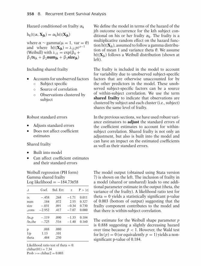
358 8. Recurrent Event Survival Analysis
Hazard conditioned on frailty αk
hk(t|α, Xjk) = αkh(t|Xjk)
where α ∼ gamma(µ = 1, var = θ)and where h(t|Xjk) = λ j k pt p−1
(Weibull) with λ j k = exp(β0 +β1txjk + β2numjk + β3sizejk)
We define the model in terms of the hazard of thejth outcome occurrence for the kth subject con-ditional on his or her frailty αk. The frailty is amultiplicative random effect on the hazard func-tion h(t|Xjk), assumed to follow a gamma distribu-tion of mean 1 and variance theta θ. We assumeh(t|Xjk) follows a Weibull distribution (shown atleft).
Including shared frailty
� Accounts for unobserved factors◦ Subject specific◦ Source of correlation◦ Observations clustered by
subject
The frailty is included in the model to accountfor variability due to unobserved subject-specificfactors that are otherwise unaccounted for bythe other predictors in the model. These unob-served subject-specific factors can be a sourceof within-subject correlation. We use the termshared frailty to indicate that observations areclustered by subject and each cluster (i.e., subject)shares the same level of frailty.
Robust standard errors
� Adjusts standard errors� Does not affect coefficientestimates
Shared frailty
� Built into model� Can affect coefficient estimatesand their standard errors
In the previous sections, we have used robust vari-ance estimators to adjust the standard errors ofthe coefficient estimates to account for within-subject correlation. Shared frailty is not only anadjustment, but also is built into the model andcan have an impact on the estimated coefficientsas well as their standard errors.
Weibull regression (PH form)Gamma shared frailtyLog likelihood = −184.73658
t Coef. Std. Err. z P > |z|
tx −.458 .268 −1.71 0.011num .184 .072 2.55 0.327size −.031 .091 −0.34 0.730cons −2.952 .417 −7.07 0.000
/ln p −.119 .090 −1.33 0.184/ln the −.725 .516 −1.40 0.160
p .888 .0801/p 1.13 .101theta .484 .250
Likelihood ratio test of theta = 0:chibar(01) = 7.34Prob >= chibar2 = 0.003
The model output (obtained using Stata version7) is shown on the left. The inclusion of frailty ina model (shared or unshared) leads to one addi-tional parameter estimate in the output (theta, thevariance of the frailty). A likelihood ratio test fortheta = 0 yields a statistically significant p-valueof 0.003 (bottom of output) suggesting that thefrailty component contributes to the model andthat there is within-subject correlation.
The estimate for the Weibull shape parameter pis 0.888 suggesting a slightly decreasing hazardover time because p < 1. However, the Wald testfor ln (p) = 0 (or equivalently p = 1) yields a non-significant p-value of 0.184.
Presentation: XI. A Second Example 359
Comparing Hazard Ratios An estimated hazard ratio of 0.633 for the effectof treatment comparing two individuals with thesame level of frailty and controlling for the othercovariates is obtained by exponentiating the es-timated coefficient (−0.458) for tx. The estimatedhazard ratio and 95% confidence intervals are sim-ilar to the corresponding results obtained usinga counting processes approach with a Cox modeland robust standard errors (see left).
Weibull with frailty model
HR(tx) = exp(−0.458) = 0.633
95% CI = exp[−0.458 ± 1.96(0.268)]
= (0.374, 1.070)
Counting processes approach withCox model
HR(tx) : exp(−0.407) = 0.667
95% CI for HR tx (robust): (0.414,1.069)
Interpretations of HR from frailtymodel
� Compares 2 individuals withsame α� Compares individual withhimself◦ What is effect if individual
had used treatment ratherthan placebo?
Another interpretation for the estimated hazardratio from the frailty model involves the compari-son of an individual to himself. In other words, thishazard ratio describes the effect on an individual’shazard (i.e., conditional hazard) if that individualhad used the treatment rather than the placebo.
XI. A Second Example We now illustrate the analysis of recurrent eventsurvival data using a new example. We consider asubset of data from the Age-Related Eye DiseaseStudy (AREDS), a long-term multicenter, prospec-tive study sponsored by the U.S. National Eye In-stitute of the clinical course of age-related mac-ular degeneration (AMD) (see AREDS ResearchGroup, 2003).
Age-Related Eye DiseaseStudy (AREDS)
Outcome
Age-related macular degeneration(AMD)
Clinical trialEvaluate effect of treatment withhigh doses of antioxidants and zincon progression of AMD
n = 43 (subset of data analyzedhere)
In addition to collecting natural history data,AREDS included a clinical trial to evaluate theeffect of high doses of antioxidants and zinc onthe progression of AMD. The data subset we con-sider consists of 43 patients who experiencedocular events while followed for their baselinecondition, macular degeneration.
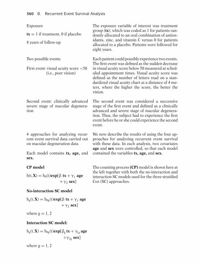
360 8. Recurrent Event Survival Analysis
Exposure
tx = 1 if treatment, 0 if placebo
8 years of follow-up
The exposure variable of interest was treatmentgroup (tx), which was coded as 1 for patients ran-domly allocated to an oral combination of antiox-idants, zinc, and vitamin C versus 0 for patientsallocated to a placebo. Patients were followed foreight years.
Two possible events
First event: visual acuity score <50(i.e., poor vision)
Each patient could possibly experience two events.The first event was defined as the sudden decreasein visual acuity score below 50 measured at sched-uled appointment times. Visual acuity score wasdefined as the number of letters read on a stan-dardized visual acuity chart at a distance of 4 me-ters, where the higher the score, the better thevision.
Second event: clinically advancedsevere stage of macular degenera-tion
The second event was considered a successivestage of the first event and defined as a clinicallyadvanced and severe stage of macular degenera-tion. Thus, the subject had to experience the firstevent before he or she could experience the secondevent.
4 approaches for analyzing recur-rent event survival data carried outon macular degeneration data
Each model contains tx, age, andsex.
We now describe the results of using the four ap-proaches for analyzing recurrent event survivalwith these data. In each analysis, two covariatesage and sex were controlled, so that each modelcontained the variables tx, age, and sex.
CP model
h(t,X) = h0(t)exp[β tx + γ1 age+γ2 sex]
No-interaction SC model
hg(t,X) = h0g(t)exp[β tx + γ1 age+γ2 sex]
where g = 1, 2
Interaction SC model:
hg(t,X) = h0g(t)exp[βg tx + γ1g age
+γ2g sex]
where g = 1, 2
The counting process (CP) model is shown here atthe left together with both the no-interaction andinteraction SC models used for the three stratifiedCox (SC) approaches.

Presentation: XI. A Second Example 361
Table 8.14. Comparison ofParameter Estimates and RobustStandard Errors for TreatmentVariable (tx) Controlling for Ageand Sex (Macular DegenerationData)
“No-“Interaction” Cox interaction”stratified model SC model
Model Stratum 1 Stratum 2β1 β2 β
(SE) (SE) (SE)Counting n/a n/a −0.174
process (0.104)Cond 1 −0.055 −0.955 −0.306
(0.286) (0.443) (0.253)Cond 2 −0.055 −1.185 −0.339
(0.286) (0.555) (0.245)Marginal −0.055 −0.861 −0.299
(0.286) (0.465) (0.290)
In Table 8.14, we compare the coefficient estimatesand their robust standard errors for the treatmentvariable (tx) from all four approaches. This tableshows results for both the “interaction” and “no-interaction” stratified Cox models for the threeapproaches other than the counting process ap-proach.
Notice that the estimated coefficients for β1 andtheir corresponding standard errors are identicalfor the three SC approaches. This will always bethe case for the first stratum regardless of the dataset being considered.
The estimated coefficients for β2 are, as expected,somewhat different for the three SC approaches.We return to these results shortly.
Interaction SC models are preferred(based on LR test results) to use ofno-interaction SC model
LR tests for comparing the “no-interaction” withthe “interaction” SC models were significant (P <
.0001) for all three SC approaches (details notshown), indicating that an interaction model wasmore appropriate than a no-interaction model foreach approach.

362 8. Recurrent Event Survival Analysis
Table 8.15. Comparison of Resultsfor the Treatment Variable (tx)Obtained for Conditional 1 andMarginal Approaches (MacularDegeneration Data)
Cond 1 Marginal
Estimate β1 −0.0555 −0.0555β2 −0.9551 −0.8615β −0.306 −0.2989
------------------------------------------------------------------------------Robust SE(β1) 0.2857 0.2857
std. SE(β2) 0.4434 0.4653error SE(β) 0.2534 0.2902
------------------------------------------------------------------------------Wald H0:β1 = 0 0.0378 0.0378
chi- H0:β2 = 0 4.6395 3.4281square H0:β = 0 1.4569 1.0609
------------------------------------------------------------------------------P-value H0:β1 = 0 0.8458 0.8478
H0:β2 = 0 0.0312 0.0641H0:β = 0 0.2274 0.3030
------------------------------------------------------------------------------Hazard exp(β1) 0.946 0.946
ratio exp(β2) 0.385 0.423exp(β) 0.736 0.742
------------------------------------------------------------------------------95% Conf. exp(β1) (0.540, 1.656) (0.540, 1.656)
interval exp(β2) (0.161, 0.918) (0.170, 1.052)exp(β) (0.448, 1.210) (0.420, 1.310)
In Table 8.15, we summarize the statistical infer-ence results for the effect of the treatment vari-able (tx) for the conditional 1 and marginal ap-proaches only.
We have not included the CP results here becausethe two events being considered are of very dif-ferent types, particularly regarding severity of ill-ness, whereas the CP approach treats both eventsas identical replications. We have not consideredthe conditional 2 approach because the investi-gators were more likely interested in survival timefrom baseline entry into the study than the sur-vival time “gap” from the first to second event.
Because we previously pointed out that the inter-action SC model was found to be significant whencompared to the corresponding no-interaction SCmodel, we focus here on the treatment (tx) effectfor each stratum (i.e., event) separately.
Based on the Wald statistics and correspondingP-values for testing the effect of the treatment onsurvival to the first event (i.e., H0: β1 = 0), both theconditional 1 and marginal approaches give theidentical result that the estimated treatment effect(HR = 0.946 = 1/1.06) is neither meaningful norsignificant (P = 0.85).
For the second event, indicating a clinically severestage of macular degeneration, the Wald statisticP-value for the conditional 1 approach is 0.03,which is significant at the .05 level, whereas thecorresponding P-value for the marginal approachis 0.06, borderline nonsignificant at the .05 level.
The estimated HR for the effect of the treatmentis HR = 0.385 = 1/2.60 using the conditional 1approach and its 95% confidence interval is quitewide but does not contain the null value of 1.For the marginal approach, the estimated HRis HR = 0.423 = 1/2.36, also with a wide confi-dence interval, but includes 1.

Presentation: XI. A Second Example 363
Conclusions regarding 1st event:
� No treatment effect� Same for conditional 1 andmarginal approaches
Thus, based on the above results, there appears tobe no effect of treating patients with high dosesof antioxidants and zinc on reducing visual acu-ity score below 50 (i.e., the first event) based oneither conditional 1 or marginal approaches tothe analysis.
Conclusions regarding 2nd event:
� Clinically moderate andstatistically significanttreatment effect� Similar for conditional 1 andmarginal approaches, but moresupport from conditional 1approach
However, there is evidence of a clinically moder-ate and statistically significant effect of the treat-ment on protection (i.e., not failing) from thesecond more severe event of macular degenera-tion. This conclusion is more supported from theconditional 1 analysis than from the marginalanalysis.
Comparison of conditional 1 withmarginal Approach
What if results had been different?
Despite similar conclusions from both ap-proaches, it still remains to compare the two ap-proaches for these data. In fact, if the results fromeach approach had been very different, it wouldbe important to make a choice between these ap-proaches.
Recommend conditional 1 if
Can assume 2nd event cannot occurwithout 1st event previouslyoccurring
⇓Should consider survival time to
2nd event conditional onexperiencing 1st event
Nevertheless, we authors find it difficult to makesuch a decision, even for this example. The con-ditional 1 approach would seem appropriate ifthe investigators assumed that the second eventcannot occur without the first event previously oc-curring. If so, it would be important to considersurvival time to the second event only for (i.e., con-ditional on) those subjects who experience a firstevent.
Recommend marginal if
Can assume each subject at risk for2nd event whether or not 1stevent previously occurred
⇓2nd event considered a separate
event, that is, unconditional ofthe 1st event
⇓Should consider survival times to
2nd event for all subjects
On the other hand, the marginal approach wouldseem appropriate if each subject is considered tobe at risk for the second event whether or notthe subject experiences the first event. The secondevent is therefore considered separate from (i.e.,unconditional of) the first event, so that survivaltimes to the second event need to be included forall subjects, as in the marginal approach.
364 8. Recurrent Event Survival Analysis
Macular degeneration data: recom-mend marginal approach
In general: carefully consider inter-pretation of each approach
For the macular degeneration data example, wefind the marginal approach persuasive. However,in general, the choice among all four approachesis not often clear-cut and requires careful consid-eration of the different interpretations that can bedrawn from each approach.
XII. Survival Curves withRecurrent Events
Goal: Plot and InterpretSurvival Curves
An important goal of most survival analyses,whether or not a regression model (e.g., Cox PH)is involved, is to plot and interpret/compare sur-vival curves for different groups. We have previ-ously described the Kaplan–Meier (KM) approachfor plotting empirical survival curves (Chapter 2)and we have also described how to obtain adjustedsurvival curves for Cox PH models (Chapters 3and 4).
Types of survival curves:
KM (empirical): Chapter 2Adjusted (Cox PH): Chapters 3 and 4
Previously: 1 (nonrecurrent) eventNow:Survival plots with recurrentevents?
This previous discussion only considered survivaldata for the occurrence of one (nonrecurrent)event. So, how does one obtain survival plots whenthere are recurrent events?
Focus on one ordered event at a time
S1(t) : 1st eventS2(t) : 2nd event
· · ·Sk(t) : kth event
The answer is that survival plots with recurrentevents only make sense when the focus is on oneordered event at a time. That is, we can plot a sur-vival curve for survival to a first event, survivalto a second event, and so on.
Survival to a 1st event
S1(t) = Pr(T1 > t)
whereT1 = survival time up to
occurrence of 1st event(ignores later recurrent events)
For survival to a first event, the survival curvedescribes the probability that a subject’s time tooccurrence of a first event will exceed a specifiedtime. Such a plot essentially ignores any recurrentevents that a subject may have after a first event.
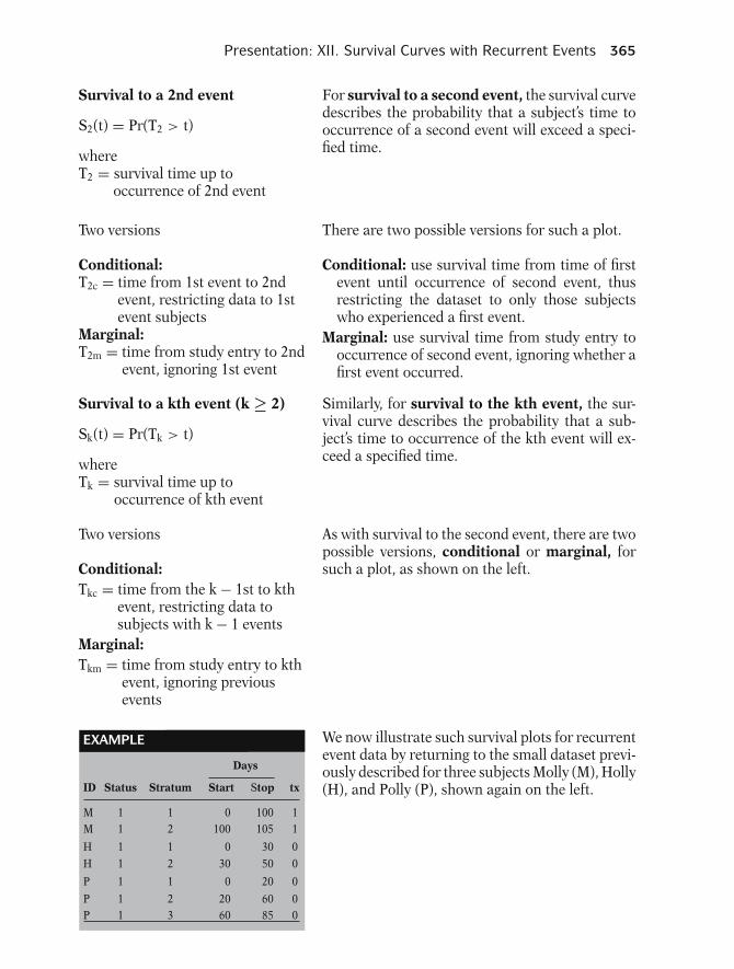
Presentation: XII. Survival Curves with Recurrent Events 365
Survival to a 2nd event
S2(t) = Pr(T2 > t)
whereT2 = survival time up to
occurrence of 2nd event
Two versions
Conditional:T2c = time from 1st event to 2nd
event, restricting data to 1stevent subjects
Marginal:T2m = time from study entry to 2nd
event, ignoring 1st event
For survival to a second event, the survival curvedescribes the probability that a subject’s time tooccurrence of a second event will exceed a speci-fied time.
There are two possible versions for such a plot.
Conditional: use survival time from time of firstevent until occurrence of second event, thusrestricting the dataset to only those subjectswho experienced a first event.
Marginal: use survival time from study entry tooccurrence of second event, ignoring whether afirst event occurred.
Survival to a kth event (k ≥ 2)
Sk(t) = Pr(Tk > t)
whereTk = survival time up to
occurrence of kth event
Similarly, for survival to the kth event, the sur-vival curve describes the probability that a sub-ject’s time to occurrence of the kth event will ex-ceed a specified time.
Two versions
Conditional:Tkc = time from the k − 1st to kth
event, restricting data tosubjects with k − 1 events
Marginal:Tkm = time from study entry to kth
event, ignoring previousevents
As with survival to the second event, there are twopossible versions, conditional or marginal, forsuch a plot, as shown on the left.
EXAMPLE
Days
ID Status Stratum Start Stop tx
M 1 11M 2 11
H 1 01
H 2 01
P 1 01
P 2 01P 3
0100
0
30
0
2060
100105
30
50
20
6085 01
We now illustrate such survival plots for recurrentevent data by returning to the small dataset previ-ously described for three subjects Molly (M), Holly(H), and Polly (P), shown again on the left.
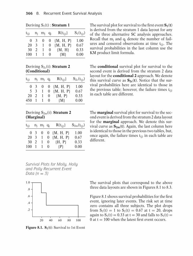
366 8. Recurrent Event Survival Analysis
Deriving S1(t) : Stratum 1
t(j) nj mj qj R(t(j)} S1(t(j))
0 3 0 0 {M, H, P} 1.0020 3 1 0 {M, H, P} 0.6730 2 1 0 {M, H} 0.33
100 1 1 0 {M} 0.00
The survival plot for survival to the first event S1(t)is derived from the stratum 1 data layout for anyof the three alternative SC analysis approaches.Recall that mj and qj denote the number of fail-ures and censored observations at time t(j). Thesurvival probabilities in the last column use theKM product limit formula.
Deriving S2c(t): Stratum 2(Conditional)
t(j) nj mj qj R(t(j)} S2c(t(j))
0 3 0 0 {M, H, P} 1.005 3 1 0 {M, H, P} 0.67
20 2 1 0 {M, P} 0.33450 1 1 0 {M} 0.00
The conditional survival plot for survival to thesecond event is derived from the stratum 2 datalayout for the conditional 2 approach. We denotethis survival curve as S2c(t). Notice that the sur-vival probabilities here are identical to those inthe previous table; however, the failure times t(j)in each table are different.
Deriving S2m(t): Stratum 2(Marginal)
t(j) nj mj qj R(t(j)} S2m(t(j))
0 3 0 0 {M, H, P} 1.0020 3 1 0 {M, H, P} 0.6730 2 1 0 {H, P} 0.33
100 1 1 0 {P} 0.00
The marginal survival plot for survival to the sec-ond event is derived from the stratum 2 data layoutfor the marginal approach. We denote this sur-vival curve as S2m(t). Again, the last column hereis identical to those in the previous two tables, but,once again, the failure times t(j) in each table aredifferent.
Survival Plots for Molly, Hollyand Polly Recurrent EventData (n = 3)
1.0
.8
.6
.4
.2
20 40 60 80 100
Figure 8.1. S1(t): Survival to 1st Event
The survival plots that correspond to the abovethree data layouts are shown in Figures 8.1 to 8.3.
Figure 8.1 shows survival probabilities for the firstevent, ignoring later events. The risk set at timezero contains all three subjects. The plot dropsfrom S1(t) = 1 to S1(t) = 0.67 at t = 20, dropsagain to S1(t) = 0.33 at t = 30 and falls to S1(t) =0 at t = 100 when the latest first event occurs.
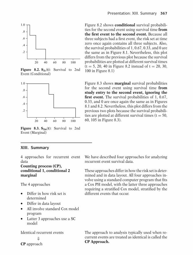
Presentation: XIII. Summary 367
1.0
.8
.6
.4
.2
20 40 60 80 100
Figure 8.2. S2c(t): Survival to 2ndEvent (Conditional)
Figure 8.2 shows conditional survival probabili-ties for the second event using survival time fromthe first event to the second event. Because allthree subjects had a first event, the risk set at timezero once again contains all three subjects. Also,the survival probabilities of 1, 0.67, 0.33, and 0 arethe same as in Figure 8.1. Nevertheless, this plotdiffers from the previous plot because the survivalprobabilities are plotted at different survival times(t = 5, 20, 40 in Figure 8.2 instead of t = 20, 30,100 in Figure 8.1)
1.0
.8
.6
.4
.2
20 40 60 80 100
Figure 8.3. S2m(t): Survival to 2ndEvent (Marginal)
Figure 8.3 shows marginal survival probabilitiesfor the second event using survival time fromstudy entry to the second event, ignoring thefirst event. The survival probabilities of 1, 0.67,0.33, and 0 are once again the same as in Figures8.1 and 8.2. Nevertheless, this plot differs from theprevious two plots because the survival probabili-ties are plotted at different survival times (t = 50,60, 105 in Figure 8.3).
XIII. Summary
4 approaches for recurrent eventdataCounting process (CP),conditional 1, conditional 2marginal
The 4 approaches
� Differ in how risk set isdetermined� Differ in data layout� All involve standard Cox modelprogram� Latter 3 approaches use a SCmodel
We have described four approaches for analyzingrecurrent event survival data.
These approaches differ in how the risk set is deter-mined and in data layout. All four approaches in-volve using a standard computer program that fitsa Cox PH model, with the latter three approachesrequiring a stratified Cox model, stratified by thedifferent events that occur.
Identical recurrent events⇓
CP approach
The approach to analysis typically used when re-current events are treated as identical is called theCP Approach.

368 8. Recurrent Event Survival Analysis
Recurrent events: different diseasecategories or event order important
⇓Stratified Cox (SC) approaches
When recurrent events involve different diseasecategories and/or the order of events is consideredimportant, the analysis requires choosing amongthe three alternative SC approaches.
CP approach: Start and Stop times
Standard layout: only Stop (sur-vival) times (no recurrent events)
The data layout for the counting process approachrequires each subject to have a line of data for eachrecurrent event and lists the start time and stoptime of the interval of follow-up. This contrastswith the standard layout for data with no recurrentevents, which lists only the stop (survival) time ona single line of data for each subject.
Conditional 1: same Start and StopTimes as CP, butuses SC model
The conditional 1 approach uses the exact same(start, stop) data layout format used for the CP ap-proach, except that for conditional 1, the modelused is a SC PH model rather than an unstratifiedPH model.
Conditional 2: Start and StopTimes
Start = 0 alwaysStop = time since
previousevent
SC model
The conditional 2 approach also uses a (start,stop) data layout, but the start value is always 0and the stop value is the time interval length sincethe previous event. The model here is also a SCmodel.
Marginal approach:
Standard layout (nonrecurrentevent), that is, without (Start,Stop) columns
Each failure is a separate process
The marginal approach uses the standard (non-recurrent event) data layout instead of the (start,stop) layout. The basic idea behind the marginalapproach is that it allows each failure to be con-sidered as a separate process.
Recommend using robust estima-tion to adjust for correlation of ob-servations on the same subject.
For each of the SC alternative approaches, as forthe CP approach, it is recommended to use ro-bust estimation to adjust the variances of the es-timated regression coefficients for the correlationof observations on the same subject.
Application 1: Bladder Cancerstudy
n = 8664 months of follow-
up
We considered two applications of the differentapproaches described above. First, we comparedresults from using all four methods to analyzedata from a study of bladder cancer involving 86patients, each followed for a variable time up to64 months.

Presentation: XIII. Summary 369
Repeated event: recurrence ofbladder cancertumor; up to4 events
The repeated event analyzed was the recurrence ofa bladder cancer tumor after transurethral surgi-cal excision. Each recurrence of new tumors wastreated by removal at each examination. About25% of the 86 subjects experienced four events.
tx = 1 if thiotepa, 0 if placebonum = initial # of tumorssize = initial size of tumors
The exposure variable of interest was drug treat-ment status (tx, 0 = placebo, 1 = treatment withthiotepa), There were two covariates: initial num-ber of tumors (num) and initial size of tumors(size).
CP results: no strong evidence for tx(HR = 0.67, P = .09, 95% CI: 0.414,1.069)
Results for the CP approach, which was consid-ered appropriate for these data, indicated thatthere was no strong evidence that tx is effectiveafter controlling for num and size (HR = 0.67,P = .09, 95% CI: 0.414, 1.069)
Alternative parametric approach
� Weibull PH model� Gamma shared frailtycomponent� Bladder cancer dataset� Similar HR and confidenceinterval as for counting processapproach
An alternative approach for analyzing recurrentevent data was also described using a parametricmodel containing a frailty component (see Chap-ter 7). Specifically, a Weibull PH model with agamma distributed frailty was fit using the blad-der cancer dataset. The resulting estimated HRand confidence interval were quite similar to thecounting process results.
Application 2: Clinical trial
n = 438 years of follow-upHigh doses of antioxidants and zincAge-related macular degeneration
The second application considered a subset of data(n = 43) from a clinical trial to evaluate the ef-fect of high doses of antioxidants and zinc on theprogression of age-related macular degeneration(AMD). Patients were followed for eight years.
Exposure: tx = 1 if treatment, 0 ifplacebo
Covariates: age, sex
The exposure variable of interest was treatmentgroup (tx). Covariates considered were age andsex.
Two possible events:
1st event: visual acuity score <50(i.e., poor vision)
2nd event: clinically advancedsevere stage of maculardegeneration
Each patient could possibly experience two events.The first event was defined as the sudden decreasein visual acuity score below 50. The second eventwas considered a successive stage of the first eventand defined as a clinically advanced and severestage of macular degeneration.

370 8. Recurrent Event Survival Analysis
Focus on conditional 1 vs.marginal (events were of differenttypes)
Because the two events were of very different typesand because survival from baseline was of primaryinterest, we focused on the results for the condi-tional 1 and marginal approaches only.
Interaction SC model ✓No-interaction SC model ×
An interaction SC model was more appropriatethan a no-interaction model for each approach,thus requiring separate results for the two eventsunder study.
Conclusions regarding 1st event
� No treatment effect� Same for conditional 1 andmarginal approaches
The results for the first event indicated no effectof the treatment on reducing visual acuity scorebelow 50 (i.e., the first event) from either condi-tional 1 or marginal approaches to the analysis.
Conclusions regarding 2nd event
� Clinically moderate andstatistically significanttreatment effect
However, there was evidence of a clinically moder-ate and statistically significant effect of the treat-ment on the second more severe event of maculardegeneration.
Macular degeneration data: prefermarginal approach (but not clear-cut)
The choice between the conditional 1 andmarginal approaches for these data was not clear-cut, although the Marginal approach was perhapsmore appropriate because the two events were ofvery different types.
In general: carefully consider inter-pretation of each approach
In general, however, the choice among all four ap-proaches requires careful consideration of the dif-ferent interpretations that can be drawn from eachapproach.
Survival plots: one ordered event ata time Two versions for survival tokth event:Conditional: only subjects with k −
1 eventsMarginal: ignores previous events
Survival plots with recurrent events are derivedone ordered event at a time. For plotting survivalto a kth event where k ≥ 2, one can use eithera conditional or marginal plot, which typicallydiffer.
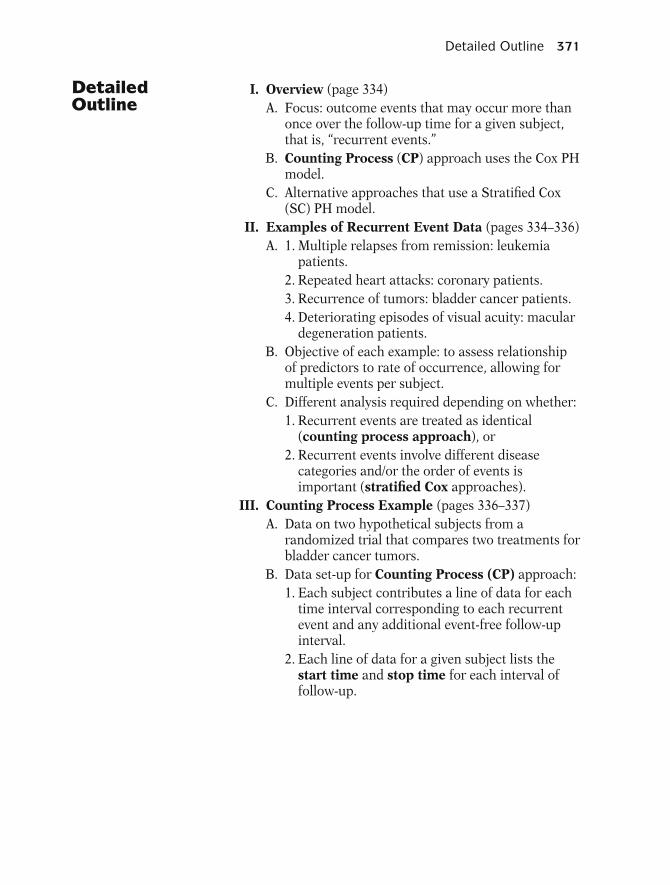
Detailed Outline 371
DetailedOutline
I. Overview (page 334)A. Focus: outcome events that may occur more than
once over the follow-up time for a given subject,that is, “recurrent events.”
B. Counting Process (CP) approach uses the Cox PHmodel.
C. Alternative approaches that use a Stratified Cox(SC) PH model.
II. Examples of Recurrent Event Data (pages 334–336)A. 1. Multiple relapses from remission: leukemia
patients.2. Repeated heart attacks: coronary patients.3. Recurrence of tumors: bladder cancer patients.4. Deteriorating episodes of visual acuity: macular
degeneration patients.B. Objective of each example: to assess relationship
of predictors to rate of occurrence, allowing formultiple events per subject.
C. Different analysis required depending on whether:1. Recurrent events are treated as identical
(counting process approach), or2. Recurrent events involve different disease
categories and/or the order of events isimportant (stratified Cox approaches).
III. Counting Process Example (pages 336–337)A. Data on two hypothetical subjects from a
randomized trial that compares two treatments forbladder cancer tumors.
B. Data set-up for Counting Process (CP) approach:1. Each subject contributes a line of data for each
time interval corresponding to each recurrentevent and any additional event-free follow-upinterval.
2. Each line of data for a given subject lists thestart time and stop time for each interval offollow-up.
372 8. Recurrent Event Survival Analysis
IV. General Data Layout for Counting ProcessApproach (pages 338–339)A. ri time intervals for subject i.
δij event status (0 or 1) for subject i in interval j.tij0 start time for subject i in interval j.tij1 stop time for subject i in interval j.Xijk value of kth predictor for subject i ininterval j.i = 1, 2,. . ., N; j = 1, 2,. . ., ni; k = 1, 2,. . ., p.
B. Layout for subject i:
i j δij tij0 tij1 Xij1 . . . Xijp
i 1 δi1 ti10 ti11 X111 . . . Xi1pi 2 δi2 ti20 ti21 X121 . . . Xi2p· · · · · · ·· · · · · · ·· · · · · · ·i ri δiri tiri0 tiri1 Xiri1 . . . Xirip
C. Bladder Cancer Study example:1. Data layout provided for the first 26 subjects
(86 subjects total) from a 64-month study ofrecurrent bladder cancer tumors.
2. The exposure variable: drug treatment status(tx, 0 = placebo, 1 = treatment with thiotepa).
3. Covariates: initial number of tumors (num) andinitial size of tumors (size).
4. Up to 4 events per subject.V. The Counting Process Model and Method
(pages 340–344)A. The model typically used to carry out the
Counting Process (CP) approach is the standardCox PH model: h(t, X) = h0(t) exp[�βiXi].
B. For recurrent event survival data, the (partial)likelihood function is formed differently than fornonrecurrent event survival data:1. A subject who continues to be followed after
having failed at t(j) does not drop out of the riskset after t(j) and remains in the risk set until hisor her last interval of follow-up, after which thesubject is removed from the risk set.
2. Different lines of data contributed by the samesubject are treated in the analysis as if they wereindependent contributions from differentsubjects.

Detailed Outline 373
C. For the bladder cancer data, the Cox PH Model forCP approach is given by
h(t, X) = h0(t)exp[β tx + γ1 num + γ2 size].
D. The overall partial likelihood L from using the CPapproach will be automatically determined by thecomputer program used once the data layout is inthe correct CP form and the program code usedinvolves the (start, stop) formulation.
VI. Robust Estimation (pages 344–346)A. In the CP approach, the different intervals
contributed by a given subject represent correlatedobservations on the same subject that must beaccounted for in the analysis.
B. A widely used technique for adjusting for thecorrelation among outcomes on the same subjectis called robust estimation.
C. The goal of robust estimation for the CPapproach is to obtain variance estimators thatadjust for correlation within subjects whenpreviously no such correlation was assumed.
D. The robust estimator of the variance of anestimated regression coefficient allows tests ofhypotheses and confidence interval estimationabout model parameters to account for correlationwithin subjects.
E. The general form of the robust estimator can bemost conveniently written in matrix notation; thisformula is incorporated into the computerprogram and is automatically calculated by theprogram with appropriate coding.
VII. Results for CP Example (pages 346–347)A. Edited output is provided from fitting the
no-interaction Cox PH model involving the threepredictors tx, num, and size.
B. A likelihood ratio chunk test for interaction termstx × num and tx × size was nonsignificant.
C. The PH assumption was assumed satisfied for allthree variables.
D. The robust estimator of 0.2418 for the standarddeviation of tx was similar though somewhatdifferent from the corresponding nonrobustestimator of 0.2001.
E. There was not strong evidence that tx is effectiveafter controlling for num and size (HR = 0.67,two-sided P = .09, 95% CI: 0.414, 1.069).
374 8. Recurrent Event Survival Analysis
F. However, for a one-sided alternative, the P-valuesusing both robust and nonrobust standard errorswere significant at the .05 level.
G. The 95% confidence interval using the robustvariance estimator is quite wide.
VIII. Other Approaches—Stratified Cox (pages 347–353)A. The “strata” variable for each of the three SC
approaches treats the time interval number foreach event occurring on a given subject as astratified variable.
B. Three alternative approaches involving SC modelsneed to be considered if the investigator wants todistinguish the order in which recurrent eventsoccur.
C. These approaches all differ from what is calledcompeting risk survival analysis in that the latterallows each subject to experience only one ofseveral different types of events over follow-up.
D. Conditional 1 approach:1. Same Start and Stop Times as CP.2. SC model.
E. Conditional 2 approach:1. Start and Stop Times, but Start = 0 always and
Stop = time since previous event.2. SC model.
F. Marginal approach:1. Uses standard layout (nonrecurrent event); no
(Start, Stop) columns.2. Treats each failure is a separate process.3. Each subject at risk for all failures that might
occur, so that # actual failures < # possiblefailures.
4. SC model.G. Must decide between two types of SC models:
1. No-interaction SC versus interaction SC.2. Bladder cancer example:
No-interaction model: hg(t,X) =h0g(t)exp[β tx + γ1 num + γ2 size]. where g =1, 2, 3, 4.Interaction model: hg(t,X) = h0g(t)exp[βgtx+ γ1gnum + γ2gsize]. where g = 1, 2, 3, 4.
H. Recommend using robust estimation to adjust forcorrelation of observations on the same subject.

Detailed Outline 375
IX. Bladder Cancer Study Example (Continued)(pages 353–357)A. Results from using all four methods—CP,
conditional 1, conditional 2, and marginal—onthe bladder cancer data were compared.
B. The hazard ratio for the effect of tx based on ano-interaction model differed somewhat for eachof the four approaches, with the marginal modelbeing most different:
M: 0.560 CP: 0.666 C1: 0.716 C2: 0.763
C. The nonrobust and robust standard errors andP-values differed to some extent for each of thedifferent approaches.
D. Using an interaction SC model, the estimated βsand corresponding standard errors are differentover the four strata (i.e., four events) for eachmodel separately.
E. The estimated β’s and corresponding standarderrors for the three alternative SC models areidentical, as expected (always for first events).
F. Which of the four recurrent event analysisapproaches is best?1. Recommend CP approach if do not want to
distinguish between recurrent events on thesame subject and desire overall conclusionabout the effect of tx.
2. Recommend one of the three SC approaches ifwant to distinguish the effect of tx according tothe order in which the event occurs.
3. The choice between the conditional 1 andmarginal is difficult, but prefer conditional 1because the strata do not clearly representdifferent event types.
G. Overall, regardless of the approach used, there wasno strong evidence that tx is effective aftercontrolling for num and size.
X. A Parametric Approach Using Shared Frailty(pages 357–359)A. Alternative approach using a parametric model
containing a frailty component (see Chapter 7).B. Weibull PH model with a gamma distributed
frailty was fit using the bladder cancer dataset.C. Estimated HR and confidence interval were quite
similar to the counting process results.D. Estimated frailty component was significant
(P = 0.003).

376 8. Recurrent Event Survival Analysis
XI. A Second Example (pages 359–364)A. Clinical trial (n = 43, 8-year study) on effect of
using high doses of antioxidants and zinc (i.e.,tx = 1 if yes, 0 if no) to prevent age-relatedmacular degeneration.
B. Covariates: age and sex.C. Two possible events:
1. First event: visual acuity score <50 (i.e., poorvision).
2. Second event: clinically advanced stage ofmacular degeneration.
D. Focus on conditional 1 vs. marginal becauseevents are of different types.
E. Interaction SC model significant when comparedto no-interaction SC model.
F. Conclusions regarding 1st event:1. No treatment effect (HR = 0.946, P = 0.85).2. Same for conditional 1 and marginal
approaches.G. Conclusions regarding 2nd event:
1. Conditional 1: HR = .385 = 1/2.60, two-sidedP = .03.
2. Marginal: HR = .423 = 1/2.36, two-sidedP = .06).
3. Overall, clinically moderate and statisticallysignificant treatment effect.
H. Marginal approach preferred because 1st and 2ndevents are different types.
XII. Survival Curves with Recurrent Events(pages 364–367)A. Survival plots with recurrent events only make
sense when the focus is on one ordered event at atime.
B. For survival from a 1st event, the survival curve isgiven by S1(t) = Pr (T1 > t) where T1 = survivaltime up to occurrence of the 1st event (ignoreslater recurrent events).
C. For survival from the kth event, the survival curveis given by Sk(t) = Pr (Tk > t) where Tk = survivaltime up to occurrence of the kth event).
Practice Exercises 377
D. Two versions for Sk(t):i. Skc(t) conditional: Tkc = time from the k − 1st
to kth event, restricting data to subjects withk − 1 events.
ii. Skm(t) marginal: Tkm = time from study entryto kth event, ignoring previous events.
E. Illustration of survival plots for recurrent eventdata using a small dataset involving three subjectsMolly (M), Holly (H), and Polly (P).
XIII. Summary (pages 367–370)A. Four approaches for analyzing recurrent event
survival data: the counting process (CP),conditional 1, conditional 2, and marginalapproaches.
B. Data layouts differ for each approach.C. CP approach uses Cox PH model; other
approaches use Cox SC model.D. Choice of approach depends in general on carefully
considering the interpretation of each approach.E. Should use robust estimation to adjust for
correlation of observations on the same subject.
PracticeExercises
Answer questions 1 to 15 as true or false (circle T or F).
T F 1. A recurrent event is an event (i.e., failure) thatcan occur more than once over the follow-up ona given subject.
T F 2. The Counting Process (CP) approach is appro-priate if a given subject can experience more thanone different type of event over follow-up.
T F 3. In the data layout for the CP approach, a subjectwho has additional follow-up time after havingfailed at time t(j) does not drop out of the risk setafter t(j).
T F 4. The CP approach requires the use of a stratifiedCox (SC) PH model.
T F 5. Using the CP approach, if exactly two subjects failat month t(j) = 10, but both these subjects havelater recurrent events, then the number in the riskset at the next ordered failure time does not de-crease because of these two failures.

378 8. Recurrent Event Survival Analysis
T F 6. The goal of robust estimation for the CPapproach is to adjust estimated regression coef-ficients to account for the correlation of obser-vations within subjects when previously no suchcorrelation was assumed.
T F 7. Robust estimation is recommended for the CPapproach but not for the alternative SC ap-proaches for analyzing recurrent event survivaldata.
T F 8. The P-value obtained from using a robust stan-dard error will always be larger than the corre-sponding P-value from using a nonrobust stan-dard error.
T F 9. The marginal approach uses the exact same(start, stop) data layout format used for the CPapproach, except that for the marginal approach,the model used is a stratified Cox PH modelvariable rather than a standard (unstratified) PHmodel.
T F 10. Supppose the maximum number of failures oc-curring for a given subject is five in a dataset tobe analyzed using the marginal approach. Then asubject who failed only twice will contribute fivelines of data corresponding to his or her two fail-ures and the three additional failures that couldhave possibly occurred for this subject.
T F 11. Suppose the maximum number of failures occur-ring for a given subject is five in a dataset tobe analyzed using the conditional 1 approach.Then an interaction SC model used to carryout this analysis will have the following gen-eral model form: hg(t, X) = h0g(t) exp[β1gX1 +β2gX2 + · · · + βpgXp], g = 1,2,3,4,5.
T F 12. Suppose a no-interaction SC model using the con-ditional 1 approach is found (using a likelihoodratio test) not statistically different from a corre-sponding interaction SC model. Then if the no-interaction model is used, it will not be possibleto separate out the effects of predictors withineach stratum representing the recurring events ona given subject.
T F 13. In choosing between the conditional 1 and themarginal approaches, the marginal approachwould be preferred provided the different strataclearly represent different event types.
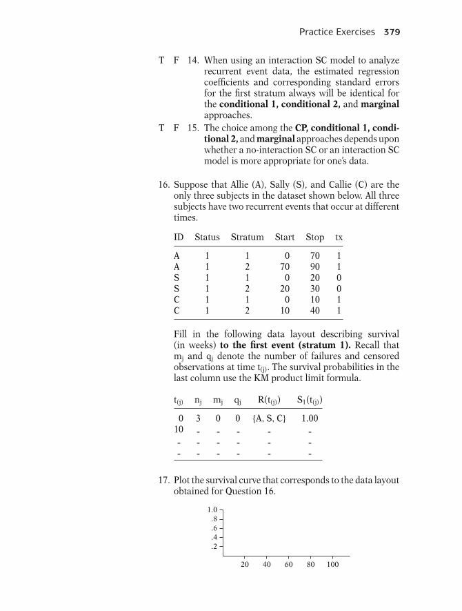
Practice Exercises 379
T F 14. When using an interaction SC model to analyzerecurrent event data, the estimated regressioncoefficients and corresponding standard errorsfor the first stratum always will be identical forthe conditional 1, conditional 2, and marginalapproaches.
T F 15. The choice among the CP, conditional 1, condi-tional 2, and marginal approaches depends uponwhether a no-interaction SC or an interaction SCmodel is more appropriate for one’s data.
16. Suppose that Allie (A), Sally (S), and Callie (C) are theonly three subjects in the dataset shown below. All threesubjects have two recurrent events that occur at differenttimes.
ID Status Stratum Start Stop tx
A 1 1 0 70 1A 1 2 70 90 1S 1 1 0 20 0S 1 2 20 30 0C 1 1 0 10 1C 1 2 10 40 1
Fill in the following data layout describing survival(in weeks) to the first event (stratum 1). Recall thatmj and qj denote the number of failures and censoredobservations at time t(j). The survival probabilities in thelast column use the KM product limit formula.
t(j) nj mj qj R(t(j)) S1(t(j))
0 3 0 0 {A, S, C} 1.0010
17. Plot the survival curve that corresponds to the data layoutobtained for Question 16.
1.0.8.6.4.2
20 40 60 80 100

380 8. Recurrent Event Survival Analysis
18. Fill in the following data layout describing survival(in weeks) from the first to second event using theconditional approach:
t(j) nj mj qj R(t(j)) S1(t(j))
0 3 0 0 {A, S, C} 1.0010
19. Plot the survival curve that corresponds to the data layoutobtained for Question 18.
1.0.8.6.4.2
20 40 60 80 100
20. Fill in the following data layout describing survival(in weeks) to the second event using the marginalapproach:
t(j) nj mj qj R(t(j)) S1(t(j))
0 3 0 0 {A, S, C} 1.0030
21. Plot the survival curve that corresponds to the data layoutobtained for Question 20.
1.0.8.6.4.2
20 40 60 80 100
22. To what extent do the three plots obtained in Questions17, 19, and 21 differ? Explain briefly.
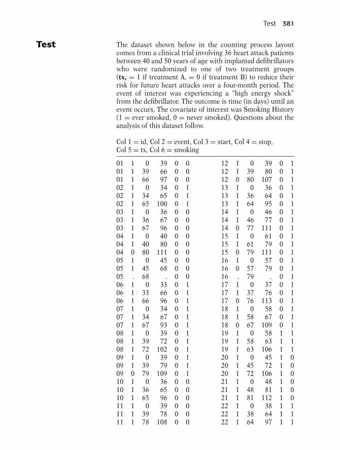
Test 381
Test The dataset shown below in the counting process layoutcomes from a clinical trial involving 36 heart attack patientsbetween 40 and 50 years of age with implanted defibrillatorswho were randomized to one of two treatment groups(tx, = 1 if treatment A, = 0 if treatment B) to reduce theirrisk for future heart attacks over a four-month period. Theevent of interest was experiencing a “high energy shock”from the defibrillator. The outcome is time (in days) until anevent occurs. The covariate of interest was Smoking History(1 = ever smoked, 0 = never smoked). Questions about theanalysis of this dataset follow.
Col 1 = id, Col 2 = event, Col 3 = start, Col 4 = stop,Col 5 = tx, Col 6 = smoking
01 1 0 39 0 0 12 1 0 39 0 101 1 39 66 0 0 12 1 39 80 0 101 1 66 97 0 0 12 0 80 107 0 102 1 0 34 0 1 13 1 0 36 0 102 1 34 65 0 1 13 1 36 64 0 102 1 65 100 0 1 13 1 64 95 0 103 1 0 36 0 0 14 1 0 46 0 103 1 36 67 0 0 14 1 46 77 0 103 1 67 96 0 0 14 0 77 111 0 104 1 0 40 0 0 15 1 0 61 0 104 1 40 80 0 0 15 1 61 79 0 104 0 80 111 0 0 15 0 79 111 0 105 1 0 45 0 0 16 1 0 57 0 105 1 45 68 0 0 16 0 57 79 0 105 . 68 . 0 0 16 . 79 . 0 106 1 0 33 0 1 17 1 0 37 0 106 1 33 66 0 1 17 1 37 76 0 106 1 66 96 0 1 17 0 76 113 0 107 1 0 34 0 1 18 1 0 58 0 107 1 34 67 0 1 18 1 58 67 0 107 1 67 93 0 1 18 0 67 109 0 108 1 0 39 0 1 19 1 0 58 1 108 1 39 72 0 1 19 1 58 63 1 108 1 72 102 0 1 19 1 63 106 1 109 1 0 39 0 1 20 1 0 45 1 009 1 39 79 0 1 20 1 45 72 1 009 0 79 109 0 1 20 1 72 106 1 010 1 0 36 0 0 21 1 0 48 1 010 1 36 65 0 0 21 1 48 81 1 010 1 65 96 0 0 21 1 81 112 1 011 1 0 39 0 0 22 1 0 38 1 111 1 39 78 0 0 22 1 38 64 1 111 1 78 108 0 0 22 1 64 97 1 1

382 8. Recurrent Event Survival Analysis
23 1 0 51 1 1 30 1 0 57 1 023 1 51 69 1 1 30 1 57 78 1 023 0 69 98 1 1 30 1 78 99 1 024 1 0 43 1 1 31 1 0 44 1 124 1 43 67 1 1 31 1 44 74 1 124 0 67 111 1 1 31 1 74 96 1 125 1 0 46 1 0 32 1 0 38 1 125 1 46 66 1 0 32 1 38 71 1 125 1 66 110 1 0 32 1 71 105 1 126 1 0 33 1 1 33 1 0 38 1 126 1 33 68 1 1 33 1 38 64 1 126 1 68 96 1 1 33 1 64 97 1 127 1 0 51 1 1 34 1 0 38 1 127 1 51 97 1 1 34 1 38 63 1 127 0 97 115 1 1 34 1 63 99 1 128 1 0 37 1 0 35 1 0 49 1 128 1 37 79 1 0 35 1 49 70 1 128 1 79 93 1 0 35 0 70 107 1 129 1 0 41 1 1 36 1 0 34 1 129 1 41 73 1 1 36 1 34 81 1 129 0 73 111 1 1 36 1 81 97 1 1
Table T.1 below provides the results for the treatment variable(tx) from no-interaction models over all four recurrent eventanalysis approaches. Each model was fit using either a CoxPH model (CP approach) or a Stratified Cox (SC) PH model(conditional 1, conditional 2, marginal approaches) thatcontrolled for the covariate smoking.
Table T.1. Comparison of Results for the Treatment Variable (tx) Obtainedfrom No-Interaction Modelsa Across Four Methods (Defibrillator Study)
Model CP Conditional 1 Conditional 2 Marginal
Parameter 0.0839 0.0046 −0.0018 −0.0043estimateb
Robust 0.1036 0.2548 0.1775 0.2579standarderror
Chi-square 0.6555 0.0003 0.0001 0.0003p-value 0.4182 0.9856 0.9918 0.9866Hazard 1.087 1.005 0.998 0.996
ratio95% confidence (0.888, 1.332) (0.610, 1.655) (0.705, 1.413) (0.601, 1.651)
interval
a No-interaction SC model fitted with PROC PHREG for the conditional 1, conditional 2 andmarginal methods; no-interaction standard Cox PH model fitted for CP approach.b Estimated coefficient of tx variable.
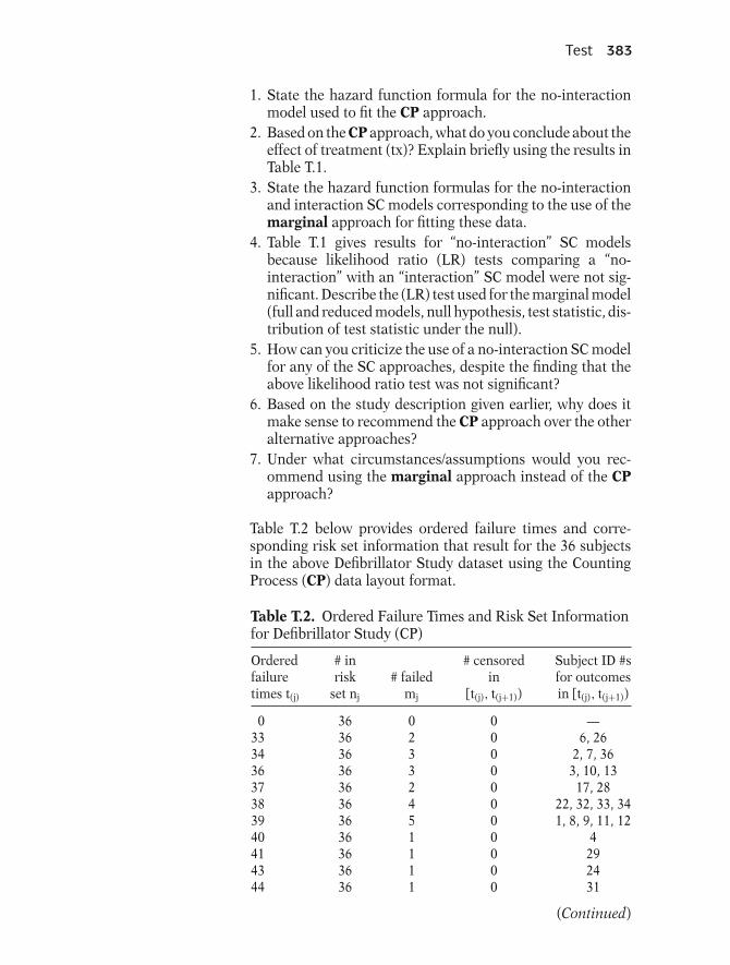
Test 383
1. State the hazard function formula for the no-interactionmodel used to fit the CP approach.
2. Based on the CP approach, what do you conclude about theeffect of treatment (tx)? Explain briefly using the results inTable T.1.
3. State the hazard function formulas for the no-interactionand interaction SC models corresponding to the use of themarginal approach for fitting these data.
4. Table T.1 gives results for “no-interaction” SC modelsbecause likelihood ratio (LR) tests comparing a “no-interaction” with an “interaction” SC model were not sig-nificant. Describe the (LR) test used for the marginal model(full and reduced models, null hypothesis, test statistic, dis-tribution of test statistic under the null).
5. How can you criticize the use of a no-interaction SC modelfor any of the SC approaches, despite the finding that theabove likelihood ratio test was not significant?
6. Based on the study description given earlier, why does itmake sense to recommend the CP approach over the otheralternative approaches?
7. Under what circumstances/assumptions would you rec-ommend using the marginal approach instead of the CPapproach?
Table T.2 below provides ordered failure times and corre-sponding risk set information that result for the 36 subjectsin the above Defibrillator Study dataset using the CountingProcess (CP) data layout format.
Table T.2. Ordered Failure Times and Risk Set Informationfor Defibrillator Study (CP)
Ordered # in # censored Subject ID #sfailure risk # failed in for outcomestimes t(j) set nj mj [t(j), t(j+1)) in [t(j), t(j+1))
0 36 0 0 —33 36 2 0 6, 2634 36 3 0 2, 7, 3636 36 3 0 3, 10, 1337 36 2 0 17, 2838 36 4 0 22, 32, 33, 3439 36 5 0 1, 8, 9, 11, 1240 36 1 0 441 36 1 0 2943 36 1 0 2444 36 1 0 31
(Continued)

384 8. Recurrent Event Survival Analysis
Table T.2. (Continued)
Ordered # in # censored Subject ID #sfailure risk # failed in for outcomestimes t(j) set nj mj [t(j), t(j+1)) in [t(j), t(j+1))
45 36 2 0 5, 2046 36 2 0 14, 2548 36 1 0 2149 36 1 0 3551 36 2 0 23, 2757 36 2 0 16, 3058 36 2 0 18, 1961 36 1 0 1563 36 2 0 19, 3464 36 3 0 13, 22, 3365 36 2 0 2, 1066 36 3 0 1, 6, 2567 36 4 0 3, 7, 18, 2468 36 2 0 5, 2669 35 1 0 2370 35 1 0 3571 35 1 0 3272 35 2 0 8, 2073 35 1 0 2974 35 1 0 3176 35 1 0 1777 35 1 0 1478 35 2 0 11, 3079 35 3 1 9, 15, 16, 2880 34 2 0 4, 1281 34 2 0 21, 3693 34 2 0 7, 2895 32 1 0 1396 31 5 0 3, 6, 10, 26, 3197 26 5 0 1, 22, 27, 33, 3698 22 0 1 2399 21 2 0 30, 34
100 19 1 0 2102 18 1 0 8105 17 1 0 32106 16 2 0 19, 20107 14 1 1 12, 35108 12 1 0 11109 11 0 2 9, 18110 9 1 0 25111 8 0 5 4, 14, 15, 24, 29112 3 1 0 21113 2 0 1 17115 1 0 1 27
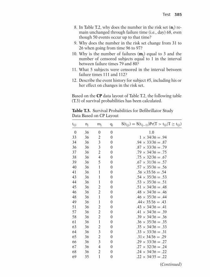
Test 385
8. In Table T.2, why does the number in the risk set (nj) re-main unchanged through failure time (i.e., day) 68, eventhough 50 events occur up to that time?
9. Why does the number in the risk set change from 31 to26 when going from time 96 to 97?
10. Why is the number of failures (mj) equal to 3 and thenumber of censored subjects equal to 1 in the intervalbetween failure times 79 and 80?
11. What 5 subjects were censored in the interval betweenfailure times 111 and 112?
12. Describe the event history for subject #5, including his orher effect on changes in the risk set.
Based on the CP data layout of Table T.2, the following table(T.3) of survival probabilities has been calculated.
Table T.3. Survival Probabilities for Defibrillator StudyData Based on CP Layout
t(j) nj mj qj S(t(j)) = S(t(j−1))Pr(T > t(j)|T ≥ t(j))
0 36 0 0 1.033 36 2 0 1 × 34/36 = .9434 36 3 0 .94 × 33/36 = .8736 36 3 0 .87 × 33/36 = .7937 36 2 0 .79 × 34/36 = .7538 36 4 0 .75 × 32/36 = .6739 36 5 0 .67 × 31/36 = .5740 36 1 0 .57 × 35/36 = .5641 36 1 0 .56 ×35/36 = .5443 36 1 0 .54 × 35/36 = .5344 36 1 0 .53 × 35/36 = .5145 36 2 0 .51 × 34/36 = .4846 36 2 0 .48 × 34/36 = .4648 36 1 0 .46 × 35/36 = .4449 36 1 0 .44× 35/36 = .4351 36 2 0 .43 × 34/36 = .4157 36 2 0 .41 × 34/36 = .3958 36 2 0 .39 × 34/36 = .3661 36 1 0 .36 × 35/36 = .3563 36 2 0 .35 × 34/36 = .3364 36 3 0 .33 × 33/36 = .3165 36 2 0 .31× 34/36 = .2966 36 3 0 .29 × 33/36 = .2767 36 4 0 .27 × 32/36 = .2468 36 2 0 .24 × 34/36 = .2269 35 1 0 .22 × 34/35 = .22
(Continued)
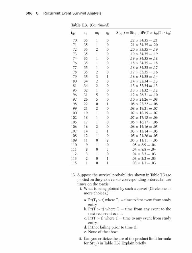
386 8. Recurrent Event Survival Analysis
Table T.3. (Continued)
t(j) nj mj qj S(t(j)) = S(t(j−1))Pr(T > t(j)|T ≥ t(j))
70 35 1 0 .22 × 34/35 = .2171 35 1 0 .21 × 34/35 = .2072 35 2 0 .20 × 33/35 = .1973 35 1 0 .19 × 34/35 = .1974 35 1 0 .19 × 34/35 = .1876 35 1 0 .18 × 34/35 = .1877 35 1 0 .18 × 34/35 = .1778 35 2 0 .17 × 33/35 = .1679 35 3 1 .16 × 31/35 = .1480 34 2 0 .14 × 32/34 = .1381 34 2 0 .13 × 32/34 = .1395 32 1 0 .13 × 31/32 = .1296 31 5 0 .12 × 26/31 = .1097 26 5 0 .10 × 21/26 = .0898 22 0 1 .08 × 22/22 = .0899 21 2 0 .08 × 19/21 = .07
100 19 1 0 .07 × 18/19 = .07102 18 1 0 .07 × 17/18 = .06105 17 1 0 .06 × 16/17 = .06106 16 2 0 .06 × 14/16 = .05107 14 1 1 .05 × 13/14 = .05108 12 1 0 .05 × 21/26 = .05109 11 0 2 .05 × 11/11 = .05110 9 1 0 .05 × 8/9 = .04111 8 0 5 .04 × 8/8 = .04112 3 1 0 .04 × 2/3 = .03113 2 0 1 .03 × 2/2 = .03115 1 0 1 .03 × 1/1 = .03
13. Suppose the survival probabilities shown in Table T.3 areplotted on the y-axis versus corresponding ordered failuretimes on the x-axis.
i. What is being plotted by such a curve? (Circle one ormore choices.)
a. Pr(T1 > t) where T1 = time to first event from studyentry.
b. Pr(T > t) where T = time from any event to thenext recurrent event.
c. Pr(T > t) where T = time to any event from studyentry.
d. Pr(not failing prior to time t).e. None of the above.
ii. Can you criticize the use of the product limit formulafor S(t(j)) in Table T.3? Explain briefly.

Test 387
14. Use Table T.2 to complete the data layouts for plotting thefollowing survival curves.a. S1(t) = Pr(T1 > t) where T1 = time to first event from
study entry
t(j) nj mj qj S(t(j)) = S(t(j−1)) × Pr(T1 > t|T1 ≥ t)
0 36 0 0 1.0033 36 2 0 0.9434 34 3 0 0.8636 31 3 0 0.7837 28 2 0 0.7238 26 4 0 0.6139 22 5 0 0.4740 17 1 0 0.4441 16 1 0 0.4243 15 1 0 0.3944 14 1 0 0.3645 13 2 0 0.3146 11 2 0 0.2548 9 1 0 0.2249 8 1 0 0.1951575861
b. Conditional S2c(t) = Pr(T2c > t) where T2c = time tosecond event from first event.
t(j) nj mj qj S(t(j)) = S(t(j−1)) × Pr(T1 > t|T1 ≥ t)
0 36 0 0 1.005 36 1 0 0.979 35 1 0 0.94
18 34 2 0 0.8920 32 1 0 0.8621 31 2 1 0.8123 28 1 0 0.7824 27 1 0 0.7525 26 1 0 0.7226 25 2 0 0.6627 23 2 0 0.6028 21 1 0 0.5829 20 1 0 0.5530 19 1 0 0.52
(Continued)

388 8. Recurrent Event Survival Analysis
(Continued)
t(j) nj mj qj S(t(j)) = S(t(j−1)) × Pr(T1 > t|T1 ≥ t)
31 18 3 0 0.4332 15 1 0 0.4033 14 5 0 0.2635 9 1 0 0.2339 8 2 0 0.174041424647
c. Marginal S2m(t) = Pr(T2m > t) where T2m = time tosecond event from study entry.
t(j) nj mj qj S(t(j)) = S(t(j−1)) × Pr(T1 > t|T1 ≥ t)
0 36 0 0 1.0063 36 2 0 0.9464 34 3 0 0.8665 31 2 0 0.8166 29 3 0 0.7267 26 4 0 0.6168 22 2 0 0.5669 20 1 0 0.5370 19 1 0 0.5071 18 1 0 0.4772 17 2 0 0.4273 15 1 0 0.3974 14 1 0 0.3676 13 1 0 0.3377 12 1 0 0.3178 11 2 0 0.2579808197
15. The survival curves corresponding to each of the data lay-outs (a, b, c) described in Question 14 will be different.Why?

Answers to Practice Exercises 389
Answers toPracticeExercises
1. T
2. F: The marginal approach is appropriate if events are ofdifferent types.
3. T
4. F: The marginal, conditional 1, and conditional 2 ap-proaches all require a SC model, whereas the CP approachrequires a standard PH model.
5. T
6. F: Robust estimation adjusts the standard errors of re-gression coefficients.
7. F: Robust estimation is recommended for all four ap-proaches, not just the CP approach.
8. F: The P-value from robust estimation may be either largeror smaller than the corresponding P-value from nonrobustestimation.
9. F: Replace the word marginal with conditional 1 or con-ditional 2. The marginal approach does not use (Start,Stop) columns in its layout.
10. T
11. T
12. T
13. T
14. T
15. F: The choice among the CP, conditional 1, conditional2, and marginal approaches depends on carefully consid-ering the interpretation of each approach.
16. t(j) nj mj qj R(t(j)} S1(t(j))
0 3 0 0 {A, S, C} 1.0010 3 1 0 {A, S, C} 0.6720 2 1 0 {A, S} 0.3370 1 1 0 {A} 0.00

390 8. Recurrent Event Survival Analysis
17. S1(t)
1.0.8.6.4.2
20 40 60 80 100
18. t(j) nj mj qj R(t(j)} S1(t(j)) Conditional
0 3 0 0 {A, S, C} 1.0010 3 1 0 {A, S, C} 0.6720 2 1 0 {A, C} 0.3330 1 1 0 {C} 0.00
19. S2c(t) Conditional
1.0.8.6.4.2
20 40 60 80 100
20. t(j) nj mj qj R(t(j)} S1(t(j)) Marginal
0 3 0 0 {A, S, C} 1.0030 3 1 0 {A, S, C} 0.6740 2 1 0 {A, C} 0.3390 1 1 0 {A} 0.00
21. S2m(t) Marginal
1.0.8.6.4.2
20 40 60 80 100
22. All three plots differ because the risk sets for each plotare defined differently inasmuch as the failure times aredifferent for each plot.
9 CompetingRisksSurvivalAnalysis
391
392 9. Competing Risks Survival Analysis
Introduction This chapter considers survival data in which each subjectcan experience only one of several different types of eventsover follow-up. This situation contrasts with the topic of thepreceding chapter in which subjects could experience morethan one event of a given type. When only one of several dif-ferent types of event can occur, we refer to the probabilitiesof these events as “competing risks,” which explains the titleof this chapter.
Modeling competing risks survival data can be carried outusing a Cox model, a parametric survival model, or modelsthat use the cumulative incidence (rather than survival). Inthis chapter, we mainly consider the Cox model because of itswide popularity and also because of the availability of com-puter programs that use the Cox model for analysis of com-peting risks.
The typical (“cause-specific”) approach for analyzing com-peting risks data is to perform a survival analysis for eachevent type separately, where the other (competing) event typesare treated as censored categories. There are two primarydrawbacks to the above method. One problem is that theabove method requires the assumption that competing risksare independent. The second problem is that the generalizedKaplan–Meier (KM)-based product-limit survival curve ob-tained from fitting separate Cox models for each event typehas questionable interpretation when there are competingrisks.
Unfortunately, if the independence assumption is incorrect,there is no direct methodology available for analyzing com-peting risks simultaneously. The only “indirect” method foraddressing this problem involves carrying out a “sensitiv-ity analysis” that treats subjects with events from compet-ing risks as all being event-free or as all experiencing theevent of interest. An example of this “sensitivity” approach isprovided.
Introduction 393
The primary alternative summary curve to the KM-based sur-vival curve is the “cumulative incidence curve (CIC),” whichestimates the “marginal probability” of an event (both termsare defined in this chapter). This CIC is not estimated usinga product-limit formulation, and its computation is not in-cluded in mainstream statistical packages. Moreover, the in-dependence of competing risks is still required when a propor-tional hazard model is used to obtain hazard ratio estimatesfor individual competing risks as an intermediate step in thecomputation of a CIC. Nevertheless, the CIC has a meaning-ful interpretation in terms of treatment utility regardless ofwhether competing risks are independent. A variation of theCIC, called the “conditional probability curve (CPC),” pro-vides a risk probability conditional on an individual not ex-periencing any of the other competing risks by time t.
An equivalent approach to the cause-specific method for an-alyzing competing risks is called the Lunn–McNeil (LM) ap-proach. The LM approach allows only one model to be fitrather than separate models for each event type and, more-over, allows flexibility to perform statistical inferences aboutsimpler versions of the LM model. This approach has addedappeal in that competing events are not considered as sim-ply being censored. Nevertheless, as with the cause-specificapproach, the LM method assumes the independence of com-peting risks.
394 9. Competing Risks Survival Analysis
AbbreviatedOutline
The outline below gives the user a preview of the materialcovered by the presentation. A detailed outline for review pur-poses follows the presentation.
I. Overview (page 396)II. Examples of Competing Risks Data
(pages 396–398)III. Byar Data (pages 399–400)IV. Method 1—Separate Models for Different Event
Types (pages 400–403)V. The Independence Assumption (pages 403–411)
VI. Cumulative Incidence Curves (CIC)(pages 412–420)
VII. Conditional Probability Curves (CPC)(pages 420–421)
VIII. Method 2—Lunn–McNeil (LM) Approach(pages 421–427)
IX. Method 2a—Alternative Lunn–McNeil (LMalt)Approach (pages 427–430)
X. Method 1—Separate Models versusMethod 2—LM Approach (pages 431–434)
XI. Summary (pages 434–439)

Objectives 395
Objectives Upon completing this chapter, the learner should be able to:
1. State or recognize examples of competing risks survivaldata.
2. Given competing risks data, outline the steps needed toanalyze such data using separate Cox models.
3. Given computer output from the analysis of competingrisk data, carry out an analysis to assess the effects ofexplanatory variables on one or more of the competingrisks.
4. State or describe the independence assumption typicallyrequired in the analysis of competing risks data.
5. Describe how to carry out and/or interpret a “sensitivityanalysis” to assess the independence assumption aboutcompeting risks.
6. State why a survival function obtained from competingrisk using the Cox model has a questionable interpreta-tion.
7. State or describe the “cumulative incidence” approachfor analyzing competing risks data.
8. Given competing risk data, describe how to calculate aCIC and/or a CPC curve.
9. Given competing risks data, outline the steps needed toanalyze such data using the Lunn–McNeil method.
10. Given computer output from fitting either a LM or LMaltmodel, carry out an analysis to assess the effect of ex-planatory variables on one or more of the competingrisks.
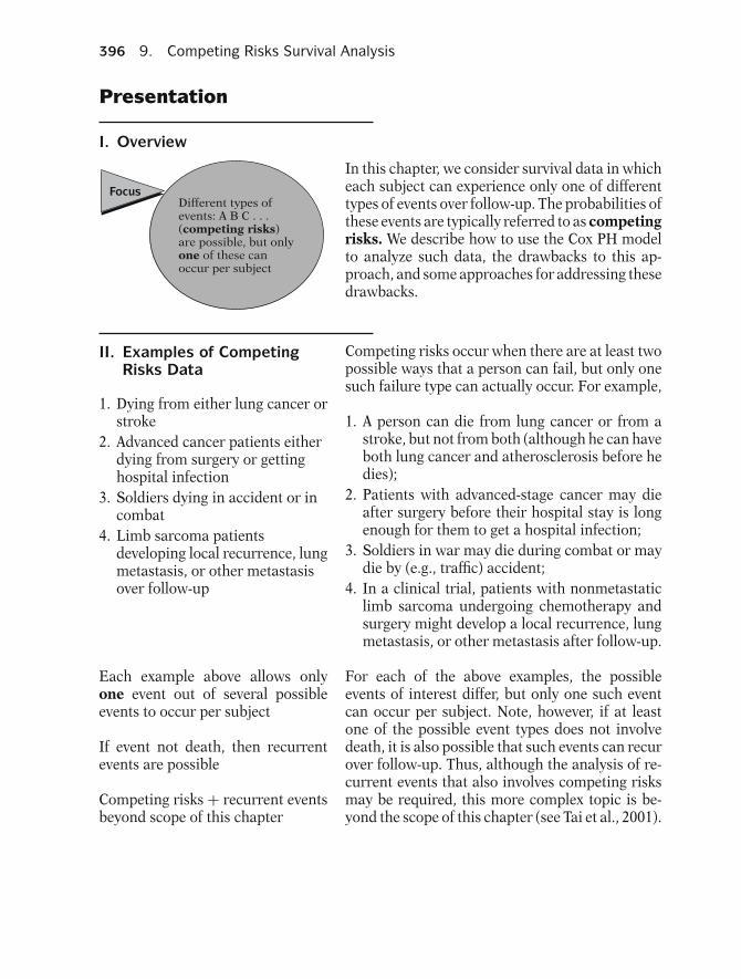
396 9. Competing Risks Survival Analysis
Presentation
I. Overview
Different types ofevents: A B C . . .(competing risks)are possible, but onlyone of these canoccur per subject
Focus
In this chapter, we consider survival data in whicheach subject can experience only one of differenttypes of events over follow-up. The probabilities ofthese events are typically referred to as competingrisks. We describe how to use the Cox PH modelto analyze such data, the drawbacks to this ap-proach, and some approaches for addressing thesedrawbacks.
II. Examples of CompetingRisks Data
1. Dying from either lung cancer orstroke
2. Advanced cancer patients eitherdying from surgery or gettinghospital infection
3. Soldiers dying in accident or incombat
4. Limb sarcoma patientsdeveloping local recurrence, lungmetastasis, or other metastasisover follow-up
Competing risks occur when there are at least twopossible ways that a person can fail, but only onesuch failure type can actually occur. For example,
1. A person can die from lung cancer or from astroke, but not from both (although he can haveboth lung cancer and atherosclerosis before hedies);
2. Patients with advanced-stage cancer may dieafter surgery before their hospital stay is longenough for them to get a hospital infection;
3. Soldiers in war may die during combat or maydie by (e.g., traffic) accident;
4. In a clinical trial, patients with nonmetastaticlimb sarcoma undergoing chemotherapy andsurgery might develop a local recurrence, lungmetastasis, or other metastasis after follow-up.
Each example above allows onlyone event out of several possibleevents to occur per subject
If event not death, then recurrentevents are possible
Competing risks + recurrent eventsbeyond scope of this chapter
For each of the above examples, the possibleevents of interest differ, but only one such eventcan occur per subject. Note, however, if at leastone of the possible event types does not involvedeath, it is also possible that such events can recurover follow-up. Thus, although the analysis of re-current events that also involves competing risksmay be required, this more complex topic is be-yond the scope of this chapter (see Tai et al., 2001).

Presentation: II. Examples of Competing Risks Data 397
Objective: assess
X1, X2, . . . , X p ⇒ Failure rate(survival probability)
for any one event allowing forcompeting risks from other possi-ble events
A logical objective for competing risks data is toassess the relationship of relevant predictors to thefailure rate or corresponding survival probabilityof any one of the possible events allowing for thecompeting risks of the other ways to fail.
Another objectiveCompare hazard rate for event Awith hazard rate for event B
We might also want to compare the failure rates(e.g., using a hazard ratio) for two or more possibleevents, controlling for relevant predictors.
Lung Cancer vs. Stroke (1)
HRLC(E vs. not E) = 1?(allowing for competing risk fromstroke)
In the lung cancer versus stroke example above, wemight ask whether the lung cancer death rate in“exposed” persons is different from the lung can-cer rate in “unexposed” persons, allowing for thepossibility that subjects could have died from astroke instead.
HR(LC vs. Stroke) = 1?(controlling for predictors)
We might also want to know if the lung cancerdeath rate differs from the stroke death rate con-trolling for predictors of interest.
Surgery Death vs. HospitalInfection (2)
HRHOSPINF(E vs. not E) = 1?(allowing for competing risk fromsurgery)
Note: death from surgery reducesnumber of hospital infections to betreated
In the second example, the competing risks aredeath from surgery versus development of a hos-pital infection. For infection control investigators,the hospital infection event is of primary inter-est. Nevertheless, the occurrence of death fromsurgery reduces the burden of hospital infectioncontrol required. Thus, the estimation of hospitalinfection rates are complicated by the competingrisk of death from surgery.
Accidental Death vs. CombatDeath (3)
HRCOMBAT (E vs. not E)(allowing competing risk of acci-dental death)
Suppose entire company dies ataccident time t before entering combat
⇓SCOMBAT(t) = P(TCOMBAT > t) = 1
where TCOMBAT = time to combat death
The third example involves competing risks ofdeath from either combat or accident in a com-pany of soldiers. Here, primary interest concernsthe hazard ratio for combat death comparing twoexposure groups. Suppose the entire company diesat time t in a helicopter accident on their way toa combat area. Because no one died in combatby time t, the survival probability of not dying incombat is one, even though no combat took place.

398 9. Competing Risks Survival Analysis
However,
TC+A = combat or accidental death
⇓“event free” SC+A(t) = P(TC+A > t) = 0
However, if we define the outcome of interest asdeath from either combat or accident, the “eventfree” survival probability is zero after the accidentoccurred (at time t).
Moreover,
SKM(TCOMBAT > t)
is undefined because the risk set isempty at time t
Moreover, the KM survival probability for combatdeath at time t is undefined because no one was atrisk for a combat death at time t.
Competing Risks Data SurvivalCurve Interpretation?
This example points out that when there are com-peting risks, the interpretation of a survival curvemay be difficult or questionable (more on this is-sue later).
Limb sarcoma patients (4)
Competing risks1 = local recurrence, 2 = lung meta-stasis, or 3 = other metastasis
HRc(E vs. not E), c = 1, 2, 3(allowing for competing risk fromother two failure types)
In the fourth example involving limb sarcoma pa-tients, the competing risks are the three failuretypes shown at the left.
In this study, the investigators wanted hazard ra-tios for each failure type, allowing for competingrisks from the other two failure types.
HR(Lung Metastasis vs. LocalRecurrence)? Controlling forPredictors
It was also of interest to compare the failure ratesfor lung metastasis versus local recurrence (or anyother two of the three failure types), controlling forrelevant predictors.
No failure types involve death⇓
Recurrent events possible
But can use classical competingrisk methods if focus on only firstfailure
Because none of the failure types involves death,recurrent events are possible for any of the threefailure types. If, however, the information on onlythe first failure is targeted, the classical competingrisk methodology described in this chapter can beapplied.

Presentation: III. Byar Data 399
III. Byar Data
� Randomized clinical trial� Compare treatments for StageIII and IV prostate cancer� Rx status: placebo or one of3 dose levels of DES
We now introduce an example of competing riskssurvival analysis of data from a randomized clini-cal trial (Byar and Green, 1980) comparing treat-ments for prostate cancer. We henceforth refer tothis as the Byar data. Patients with Stages III(local extension beyond the prostate gland) andIV (distant metastases, elevated acid phosphatase,or both) prostate cancer were randomized to re-ceive either a placebo or one of three dose levels ofthe active treatment diethylstilbestrol (DES).
Competing risks: deaths from
Cancer (main focus)CVDOther
Covariate information collected
Some predictors grouped
In this study, patients could die from prostate can-cer, cardiovascular disease, or other causes. Co-variate information was also collected to accountfor the possible influence of predictors on survival.These data have been analyzed extensively (Byarand Corle, 1977, Kay, 1986, and Lunn and McNeil,1995). Some grouping of the predictors was con-sidered to be clinically meaningful.
Predictors Value Category
Treatment (Rx) 0 Placebo, 0.2 mg DES1 1.0, 5 mg DES
Age at diagnosis 0 ≤74 yearsDiagnosis (Age) 1 75–79 years
2 ≥80 yearsStandardizeda 0 ≥100
weight (Wt) 1 80–992 <80
Performance 0 Normalstatus (PF) 1 Limitation of activity
History of 0 NoCVD (Hx) 1 Yes
Hemoglobin (Hg) 0 ≥12 g/100 ml1 9.0–11.9 g/100 ml2 <9 g/100 ml
Size of the primary 0 <30 cm2
lesion (SZ) 1 ≥30 cm2
Gleeson 0 ≤10Score+(SG) 1 >10
a weight (kg) − height (cm) + 200+ index of tumor invasiveness/aggressiveness
Key risk factors related to the primary outcomeof interest (cancer deaths) and the appropriategrouping is shown at the left.
Primary interest was to assess the effect of treat-ment (Rx) adjusted for relevant risk factors in thepresence of the competing risks. Notice from thetable that the Rx variable is grouped into a binaryvariable by coding subjects receiving the placeboor 0.2 mg of DES as 0 and coding subjects receiv-ing 1.0 or 5.0 mg of DES as 1.

400 9. Competing Risks Survival Analysis
Independence assumption (dis-cussed later)Next
Analysis of competing riskssurvival data
Assume independentcompeting risks
From a clinical perspective, these three competingrisks can be considered to be independent (e.g.,failure from heart disease and/or other causes ofdeath is unrelated to risk of failure from prostatecancer). We discuss this “independence assump-tion” in more detail in a subsequent section of thischapter.
We now describe the approach typically used toanalyze competing risks data. This approach as-sumes that competing risks are independent. Weillustrate this approach using the Byar data.
IV. Method 1—SeparateModels for DifferentEvent Types
� Use Cox (PH) model� Estimate separate hazards orHRs for each failure type� Other (competing) failure typesare treated as censored� Persons lost to follow-up orwithdrawal are also censored
The typical approach for analyzing competingrisks data uses the Cox (PH) model to separatelyestimate hazards and corresponding hazard ratiosfor each failure type, treating the other (compet-ing) failure types as censored in addition to thosewho are censored from loss to follow-up or with-drawal. We refer to this approach as Method 1because we later describe an alternative approach(Method 2) that requires only a single model to befit.
If only one failure type of interest⇓
Estimate only one hazard or HR
If only one failure type is of primary interest, thenthe analysis might be restricted to estimating haz-ards or hazard ratios for that type only (but stilltreating the competing failure types as censored).
Cause-specific hazard function
hc(t) = lim�t→0
P(t ≤ Tc < t + �t|Tc ≥ t)/�t
where Tc = time-to-failure fromevent cc = 1, 2, . . . , C (# of event types)
To describe this method mathematically, we definethe cause-specific hazard function shown at theleft. The random variable Tc denotes the time-to-failure from event type c. Thus, hc(t) gives the in-stantaneous failure rate at time t for event type c,given not failing from event c by time t.
Cox PH cause-specific model(event-type c):
hc(t,X) = h0c(t)exp[p∑
i=1
βicXi],
c = 1, . . . , C
βic allows effect of Xi to differ byevent-type
Using a Cox PH model that considers predictorsX = (X1, X2, . . . , Xp), the cause-specific hazardmodel for event type c has the form shown at theleft. Note that βic, the regression coefficient for theith predictor, is subscripted by c to indicate thatthe effects of the predictors may be different fordifferent event types.
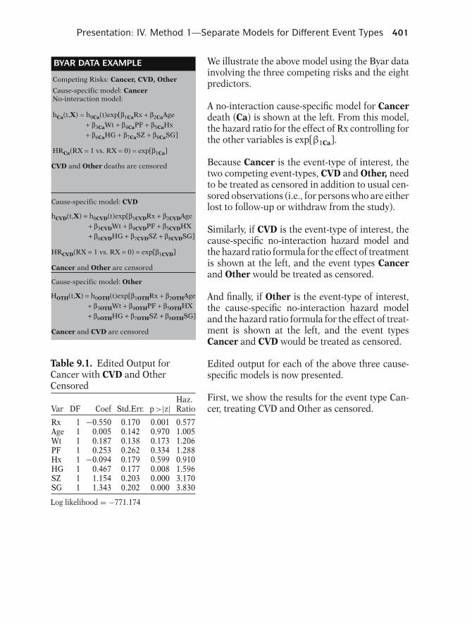
Presentation: IV. Method 1—Separate Models for Different Event Types 401
BYAR DATA EXAMPLE
Cause-specific model: CancerNo-interaction model:
hCa(t,X) = h0Ca(t)exp[β1CaRx + β2CaAge
+ β3CaWt + β4CaPF + β5CaHx
+ β6CaHG + β7CaSZ + β8CaSG]
HRCa(RX = 1 vs. RX = 0) = exp[β1Ca]
CVD and Other deaths are censored
Cause-specific model: CVD
Cause-specific model: Other
hCVD(t,X) = h0CVD(t)exp[β1CVDRx + β2CVDAge
+ β3CVDWt + β4CVDPF + β5CVDHX
+ β6CVDHG + β7CVDSZ + β8CVDSG]
HRCVD(RX = 1 vs. RX = 0) = exp[β1CVD]
Cancer and Other are censored
Cancer and CVD are censored
HOTH(t,X) = h0OTH(t)exp[β1OTHRx + β2OTHAge
+ β3OTHWt + β4OTHPF + β5OTHHX
+ β6OTHHG + β7OTHSZ + β8OTHSG]
Competing Risks: Cancer, CVD, Other
We illustrate the above model using the Byar datainvolving the three competing risks and the eightpredictors.
A no-interaction cause-specific model for Cancerdeath (Ca) is shown at the left. From this model,the hazard ratio for the effect of Rx controlling forthe other variables is exp[β1Ca].
Because Cancer is the event-type of interest, thetwo competing event-types, CVD and Other, needto be treated as censored in addition to usual cen-sored observations (i.e., for persons who are eitherlost to follow-up or withdraw from the study).
Similarly, if CVD is the event-type of interest, thecause-specific no-interaction hazard model andthe hazard ratio formula for the effect of treatmentis shown at the left, and the event types Cancerand Other would be treated as censored.
And finally, if Other is the event-type of interest,the cause-specific no-interaction hazard modeland the hazard ratio formula for the effect of treat-ment is shown at the left, and the event typesCancer and CVD would be treated as censored.
Table 9.1. Edited Output forCancer with CVD and OtherCensored
Haz.Var DF Coef Std.Err. p >|z| Ratio
Rx 1 −0.550 0.170 0.001 0.577Age 1 0.005 0.142 0.970 1.005Wt 1 0.187 0.138 0.173 1.206PF 1 0.253 0.262 0.334 1.288Hx 1 −0.094 0.179 0.599 0.910HG 1 0.467 0.177 0.008 1.596SZ 1 1.154 0.203 0.000 3.170SG 1 1.343 0.202 0.000 3.830
Log likelihood = −771.174
Edited output for each of the above three cause-specific models is now presented.
First, we show the results for the event type Can-cer, treating CVD and Other as censored.
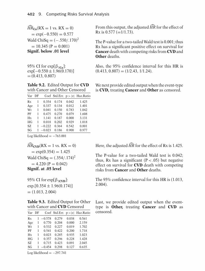
402 9. Competing Risks Survival Analysis
HRCa(RX = 1 vs. RX = 0)= exp(−0.550) = 0.577
Wald ChiSq = (−.550/.170)2
= 10.345 (P = 0.001)Signif. below .01 level
95% CI for exp[β1Ca]:exp[−0.550 ± 1.96(0.170)]= (0.413, 0.807)
From this output, the adjusted HR for the effect ofRx is 0.577 (=1/1.73).
The P-value for a two-tailed Wald test is 0.001; thusRx has a significant positive effect on survival forCancer death with competing risks from CVD andOther deaths.
Also, the 95% confidence interval for this HR is(0.413, 0.807) = (1/2.43, 1/1.24).
Table 9.2. Edited Output for CVDwith Cancer and Other CensoredVar DF Coef Std.Err. p > |z| Haz.Ratio
Rx 1 0.354 0.174 0.042 1.425Age 1 0.337 0.134 0.012 1.401Wt 1 0.041 0.150 0.783 1.042PF 1 0.475 0.270 0.079 1.608Hx 1 1.141 0.187 0.000 3.131HG 1 0.018 0.202 0.929 1.018SZ 1 −0.222 0.364 0.542 0.801SG 1 −0.023 0.186 0.900 0.977
Log likelihood = −763.001
We next provide edited output when the event-typeis CVD, treating Cancer and Other as censored.
HRCVD(RX = 1 vs. RX = 0)= exp(0.354) = 1.425
Wald ChiSq = (.354/.174)2
= 4.220 (P = 0.042)Signif. at .05 level
Here, the adjusted HR for the effect of Rx is 1.425.
The P-value for a two-tailed Wald test is 0.042;thus, Rx has a significant (P < .05) but negativeeffect on survival for CVD death with competingrisks from Cancer and Other deaths.
95% CI for exp[β1CVD]:exp.[0.354 ± 1.96(0.174)]= (1.013, 2.004)
The 95% confidence interval for this HR is (1.013,2.004).
Table 9.3. Edited Output for Otherwith Cancer and CVD CensoredVar DF Coef Std.Err. p >|z| Haz.Ratio
Rx 1 −0.578 0.279 0.038 0.561Age 1 0.770 0.204 0.000 2.159Wt 1 0.532 0.227 0.019 1.702PF 1 0.541 0.422 0.200 1.718Hx 1 0.023 0.285 0.935 1.023HG 1 0.357 0.296 0.228 1.428SZ 1 0.715 0.423 0.091 2.045SG 1 −0.454 0.298 0.127 0.635
Log likelihood = −297.741
Last, we provide edited output when the event-type is Other, treating Cancer and CVD ascensored.
Presentation: V. The Independence Assumption 403
HRCOTH(RX = 1 vs. RX = 0)= exp(−0.580) = 0.561
Wald ChiSq = (−.578/.279)2
= 4.29 (P = 0.038)Signif. at .05 level
Here, the adjusted HR for the effect of Rx is 0.561(= 1/1.78).
The P-value for a two-tailed Wald test is .038; thus,Rx has a significant (P < .05) protective effect onsurvival for Other deaths with competing risksfrom Cancer and CVD deaths.
95% CI for exp[β1OTH]:exp .[−0.578 ± 1.96(0.279)]= (0.325, 0.969)
The 95% confidence interval for this HR is (0.325,0.969), which is somewhat imprecise.
Not assessed in the above analysis:
PH assumption
Interaction of Rx with control vari-ables
We have thus completed a competing risk analy-sis of the Byar data assuming that a no-interactionCox PH model is appropriate. We haven’t actuallychecked the PH assumption for any of the vari-ables in the model nor have we assessed whetherthere is significant interaction between Rx and theother variables being controlled. Typically, thesesituations should be explored to ensure a moreappropriate analysis.
V. The IndependenceAssumption
Censoring: a major concern insurvival analysis
Right Censoring vs. left censoring↓� More often� Our focus
At the beginning of this text in Chapter 1, we intro-duced the concept of censoring as a major concernfor the analysis of survival data. We distinguishedbetween right- and left-censoring and indicatedour focus in the text would be on right-censoring,which occurs more often.
Important assumption
� Required for all approaches/models described to this point� Relevant for competing risks
We also briefly introduced in Chapter 1 an impor-tant assumption about censoring that is requiredfor all approaches/models for analyzing survivaldata described up to this point, including datawith competing risks. This assumption is typicallystated as follows: censoring is noninformative orindependent.
Censoring Is Noninformative(Synonym: Independent)

404 9. Competing Risks Survival Analysis
Typical context
� No competing risks� Homogeneous sample
Noninformative censoring can be defined in a con-text that assumes the absence of competing risksand a homogeneous study sample; that is, all sub-jects have the same values for covariate predictors.
Definition: noninformative censor-ing:
Probability of being censored attime t does not depend on prog-nosis for failure at time t
In the above context, we define noninformativecensoring to mean that the probability of beingcensored for any subject in the risk set at time tdoes not depend on that subject’s prognosis forfailure at time t.
EXAMPLEHarry in homogeneous risk set at time t
Event: death from any cause
Suppose, for example, that Harry is in a homoge-neous risk set at time t (e.g., the entire risk set is,say, white, male, age 60) and the event of interestis death from any cause, so there are no competingrisks.
3 possible outcomes at time tFail, not fail, unknown (censored)status
Given the above scenario, one of the followingthree outcomes can be observed on each subject,including Harry, in the risk set at time t: he canfail (i.e., die), not fail, or have unknown (censored)outcome from withdrawal or loss to follow-up.
Harry in poorer health than othersubjects in risk set at time t
⇓Harry’s prognosis for failing higherthan other subjects in the risk set attime t
Now, suppose Harry is in much poorer healththan other subjects in the risk set at time t. ThenHarry’s potential for failing at time t is likely tobe higher than for other subjects in the risk set attime t.
Noninformative censoring⇓⇑
Pr (C | PH) = Pr(C | GH)where
C = censoringPH = poor healthGH = good health
Now, if censoring is noninformative, then de-spite Harry’s being in poorer health than othersubjects at time t, a subject like Harry wouldjust as likely be censored as any other sub-ject in the risk set, including subjects healthierthan Harry who have a lower prognosis for failure.
Presentation: V. The Independence Assumption 405
Harry more likely to be censoredthan other subjects in risk set
⇓Pr(C | PH) > Pr(C | GH)
⇓⇑
Nevertheless, because Harry has poor health, hemight be more likely to drop out of the study (i.e.,be censored) at time t because of his poor healththan other healthier subjects in the risk set. Ifso, Harry’s censoring would be informative (ordependent).
Informative censoring unfortunately can lead tobiased results in a survival analysis. A bias canresult because people who get censored are morelikely to have failed than those not censored. Thus,the estimated survival probability at any time tmay overestimate the true survival probability attime t if a large proportion of those with unknownstatus (i.e., censored) actually failed.
Informative Censoring(Synonym: DEPENDENT)
⇓Biased results
S(t) overestimates S(t)if
large proportion of censored sub-jects actually failed at time t
Competing risks⇓
Different types of censoring
� Failure from competing risks� Lost to follow-up� Withdrawal� End of study
When the survival analysis problem involves com-peting risks, the requirement of noninformativeor independent censoring has the additionalcomplication that there are different types of cen-soring that are possible. That is, when focusingon the cause-specific hazard for event-type A, say,competing risks other than A are also consideredas censored in addition to standard censorshipfrom lost to follow-up, withdrawal, or ending ofthe study.
Noninformative (i.e.,Independent) Censoring withCompeting Risks
Harry in risk set at time t⇓
Harry just as likely to be censoredas any other subject in risk setregardless of reason for censoringor prognosis for event-type A
Thus, for competing risks, censoring is noninfor-mative or independent if for a subject like Harryin the risk set at time t, Harry is just as likely to becensored at time t as any other subject in the riskset at t, regardless of the reason for censoring, in-cluding failure from a competing risk, or Harry’sprognosis for failing from event-type A.
Byar data: 3 competing risks(Cancer, CVD, Other deaths)
Noninformative censoring?
For example, in the Byar data set, there werethree competing risks of interest, Cancer, CVD,or Other deaths. What, then, must we assume ifcensoring in this study were noninformative?

406 9. Competing Risks Survival Analysis
Cause-specific focus: CancerNoninformative censoring
⇓Harry just as likely to be censored
as any other subject in risk setregardless of type of censoring
Types of censoring—competing risks:CVD or Other death or usual censoring
Suppose censoring is noninformative and wefocus on cause-specific deaths for Cancer. Thenany subject (e.g., Harry) in the risk set at time twith a given set of covariates is just as likely tobe censored at time t as any other subject in therisk set with the same set of covariates regard-less of whether the reason for censoring is a CVDor Other death, withdrawal from study, or loss tofollow-up.
Informative (Dependent)Censoring
Harry in poorer health than othersubjects in risk set at time t
⇓Harry more likely to be censored
than other subjects in risk set
On the other hand, if censoring is informative(or dependent) and Harry was in poorer healththan other subjects in the risk set at time t, hemight be more likely to be censored, including dy-ing from CVD or Other cause, at time t than othersubjects in the risk set.
Initial context: subjects are homoge-neous
More general context: each subjectrepresentative of subjects in the riskset with the same values of predic-tors
Recall that the context in which we initially de-fined noninformative censoring assumed subjectsin the risk set at time t to be “homogeneous,” thatis, having the same values for the predictors ofinterest. Actually, because predictors are typicallyincluded in one’s model, the more general contextassumes that each subject in the risk set at time t isrepresentative of all subjects with the same valuesof the predictors who survive to time t.
EXAMPLEE = exposed, Age = 45, Gender = male
Noninformative censoring
All subjects in risk set for whichE = exposed, Age = 45, Gender = male are equally likely to be censored regardless of type of censoring
⇓
For example, if the predictors are exposure (E),Age, and Gender, then noninformative censoringrequires that a subject in the risk set at time t whois exposed, 45 years old, and male, is just as likelyto be censored at time t as any other subject inthe risk set at time t who is also exposed, 45 yearsold, and male.
Presentation: V. The Independence Assumption 407
Important assumption forcompeting risks
Censoring is noninformative (i.e.,independent)regardless of different types ofcensoring possible
Synonym: Competing risks areindependent
The important message at this point when ana-lyzing competing risks survival data is that it istypically assumed that censoring is noninforma-tive or independent regardless of the differentways that censoring can occur, including failurefrom competing risks other than the cause-specificevent-type of interest. A synonymous expressionis to say that competing risks are independent,which we henceforth adopt in our remaining dis-cussion of this topic.
Questions about independence as-sumption
1. How can we determine whetherthis assumption is satisfied?
2. How can we proceed with theanalysis to consider thepossibility that the assumptionis not satisfied?
So, if we typically require that competing risks areindependent, (1) how can we determine whetherthis assumption is satisfied and (2) how can weproceed with the analysis to consider the possibil-ity that the assumption is not satisfied?
Answer to 1:We can never explicitly prove the
assumption is satisfied for givendata.
For example, Byar data: CancerdeathThen can’t determine would havedied from Cancer if hadn’t diedfrom CVD.
CVD death⇓
Cancer death unobservable
Unfortunately, the answer to the first question isthat we can never explicitly prove that compet-ing risks are or are not independent for a givendataset. For example, in the Byar dataset, we can-not determine for certain whether a subject whodied from, say, CVD at time t would have died fromCancer if he hadn’t died from CVD.
In generalFailure from competing risk A
⇓Failure from competing risk B
unobservable
In other words, dying from Cancer at time t is anunobservable outcome for a subject who died fromCVD at or before time t. More generally, failurefrom a competing risk at time t is unobservable fora subject who has already failed from a differentcompeting risk up to time t.
Answer to 2:Alternative strategies available
but no strategy is always best
Because we can never fully determine whethercompeting risks are independent, how can we pro-ceed with the analysis of competing risks survivaldata? The answer is that there are several alterna-tive strategies, but no one strategy that is alwaysbest.

408 9. Competing Risks Survival Analysis
Strategy 1Decide assumption satisfied onclinical/biological/other grounds
One strategy is to decide on clinical/biological/other grounds without any data analysis that theindependence assumption is satisfied and thencarry out the analysis assuming independence.
EXAMPLE OF STRATEGY 1—CANCER VS. CVDDecide independence if subjects who werecensored because of CVD death were nomore or less likely to have died fromCancer.
For example, suppose the two competing risks areCancer deaths and CVD deaths. Then you maydecide that the assumption of independent com-peting risks is reasonable if at any time t, subjectswho were censored because of CVD death were nomore or less likely to have died from Cancer.
Strategy 2Include common risk factors forcompeting risks in survival model
EXAMPLE OF STRATEGY 2—CANCER VS. CVDInclude age smoking in model toremove the common effects of thesevariables on competing risks
A second strategy is to measure those variablesthat are common risk factors for competing risksbeing considered and then include those variablesin the survival model. For example, with Cancerand CVD, perhaps including age and smoking sta-tus in the survival model might remove commoneffects on competing risks.
Criticism of Strategies 1 and 2Assumptions cannot beverified with observed data
A criticism of each of the above strategies is thatthey both rely on assumptions that cannot be ver-ified with the observed data.
Strategy 3Use a sensitivity analysis
� Considers “worst-case”violations of theindependence assumption
Another strategy (3) that can be used is a sensitiv-ity analysis. As with Strategies 1 and 2, a sensitiv-ity analysis cannot explicitly demonstrate whetherthe independence assumption is satisfied. How-ever, this strategy allows the estimation of param-eters by considering “worst-case” violations of theindependence assumption.
Sensitivity analysis
� Determines extreme ranges forestimated parameters of one’smodel
Thus, using a sensitivity analysis, the investigatorcan determine extreme ranges for the estimatedparameters in one’s model under violation of theindependence assumption.
If “worst-case” not meaningfullydifferent from independence
thenat most a small bias whenassuming independence
If such “worst-case” results do not meaningfullydiffer from results obtained under the indepen-dence assumption, then the investigator mayconclude that at most a small bias can result froman analysis that assumes independence.

Presentation: V. The Independence Assumption 409
If “worst-case” meaningfullydifferent from independence
thenonly extreme of bias but notactual bias is determined
If, on the other hand, the sensitivity analysis pro-vides results that meaningfully differ from resultsobtained under the independence assumption, theinvestigator learns only the extremes to whichthe results could be biased without adjustingfor the actual bias.
EXAMPLE BYAR DATA
Cause-specific focus: CancerCensored: CVD deaths, Other deaths,
usual censoring
Worst-case situations:
1. CVD or Other deaths are assumed to die of cancer instead2. CVD or Other deaths assumed to survive as long as the largest survival time observed in the study
We now illustrate how a sensitivity analysis can becarried out using the Byar data, where we focuson the cause-specific survival for Cancer deaths,treating CVD and Other deaths as censored in ad-dition to usual censoring.
The following two worst-case situations are con-sidered. (1) All subjects that are censored becauseof CVD or Other deaths are assumed to die of can-cer instead. (2) All subjects that are censored be-cause of CVD or Other deaths survive as long asthe largest survival time observed in the study.
Table 9.4. Edited Output forCancer Worst-Case (1)Var DF Coef Std.Err. p >|z| Haz.Ratio
Rx 1 −0.185 0.110 0.092 0.831Age 1 0.286 0.087 0.001 1.332Wt 1 0.198 0.093 0.032 1.219PF 1 0.402 0.170 0.018 1.495Hx 1 0.437 0.112 0.000 1.548HG 1 0.292 0.120 0.015 1.339SZ 1 0.672 0.159 0.000 1.958SG 1 0.399 0.115 0.001 1.491
Log likelihood = −1892.091
Table 9.5. Edited Output forCancer Worst-Case (2)
Haz.Var DF Coef Std.Err. p >|z| Ratio
Rx 1 −0.411 0.169 0.015 0.663Age 1 −0.118 0.139 0.394 0.888Wt 1 0.086 0.138 0.532 1.090PF 1 0.125 0.254 0.622 1.133Hx 1 −0.266 0.179 0.138 0.767HG 1 0.314 0.169 0.063 1.369SZ 1 0.825 0.197 0.000 2.282SG 1 1.293 0.201 0.000 3.644
Log likelihood = −839.631
Table 9.4 and Table 9.5 give edited output for theabove two scenarios followed by a repeat of theoutput previously shown (Table 9.1) under the in-dependence assumption.
To carry out worst-case scenario (1), the Statusvariable (indicating whether a subject failed orwas censored) was changed in the dataset from0 to 1 for each subject that had a CVD or Otherdeath.
For worst-case scenario (2), the longest survivaltime observed in the study was 76 weeks. Thus,the survival time for each subject that had a CVDor Other death was changed in the dataset fromthe actual time of death to 76 weeks.
To evaluate the results of the sensitivity analysis,we need to compare the output in Table 9.1, whichassumes that competing risks are independent,with output for worst-case situations provided inTable 9.4 and Table 9.5. We focus this compari-son on the estimated coefficient of the Rx variable.
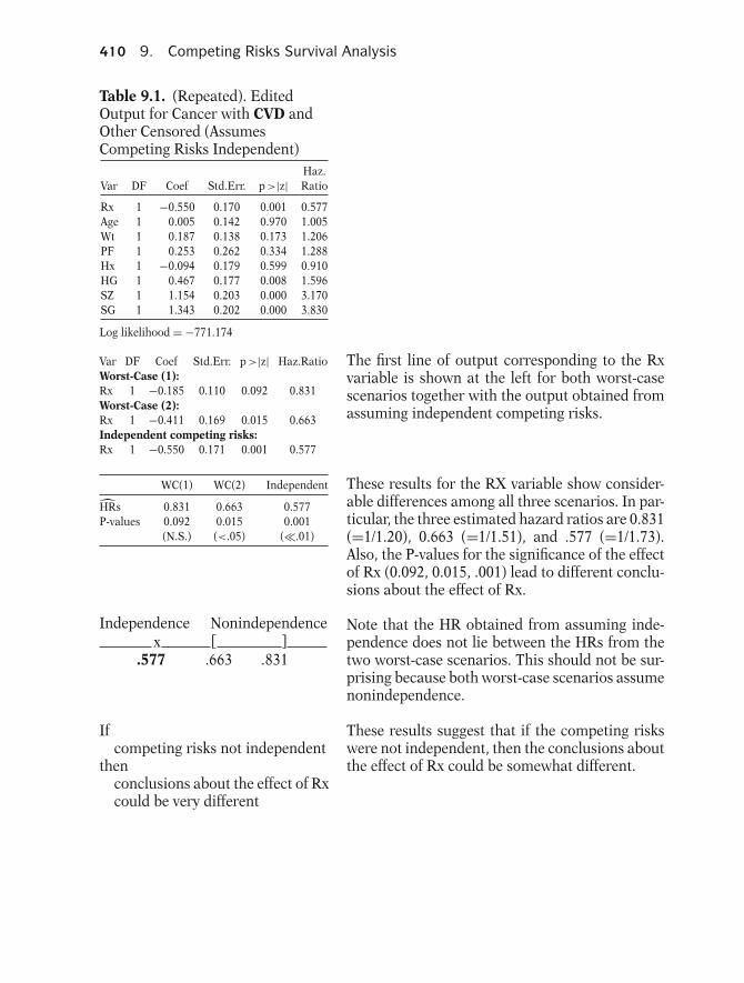
410 9. Competing Risks Survival Analysis
Table 9.1. (Repeated). EditedOutput for Cancer with CVD andOther Censored (AssumesCompeting Risks Independent)
Haz.Var DF Coef Std.Err. p >|z| Ratio
Rx 1 −0.550 0.170 0.001 0.577Age 1 0.005 0.142 0.970 1.005Wt 1 0.187 0.138 0.173 1.206PF 1 0.253 0.262 0.334 1.288Hx 1 −0.094 0.179 0.599 0.910HG 1 0.467 0.177 0.008 1.596SZ 1 1.154 0.203 0.000 3.170SG 1 1.343 0.202 0.000 3.830
Log likelihood = −771.174
Var DF Coef Std.Err. p >|z| Haz.RatioWorst-Case (1):Rx 1 −0.185 0.110 0.092 0.831Worst-Case (2):Rx 1 −0.411 0.169 0.015 0.663Independent competing risks:Rx 1 −0.550 0.171 0.001 0.577
The first line of output corresponding to the Rxvariable is shown at the left for both worst-casescenarios together with the output obtained fromassuming independent competing risks.
WC(1) WC(2) Independent
HRs 0.831 0.663 0.577P-values 0.092 0.015 0.001
(N.S.) (<.05) (�.01)
These results for the RX variable show consider-able differences among all three scenarios. In par-ticular, the three estimated hazard ratios are 0.831(=1/1.20), 0.663 (=1/1.51), and .577 (=1/1.73).Also, the P-values for the significance of the effectof Rx (0.092, 0.015, .001) lead to different conclu-sions about the effect of Rx.
Independence Nonindependencex [ ]
.577 .663 .831
Note that the HR obtained from assuming inde-pendence does not lie between the HRs from thetwo worst-case scenarios. This should not be sur-prising because both worst-case scenarios assumenonindependence.
Ifcompeting risks not independent
thenconclusions about the effect of Rxcould be very different
These results suggest that if the competing riskswere not independent, then the conclusions aboutthe effect of Rx could be somewhat different.

Presentation: V. The Independence Assumption 411
But,
� Have not demonstrated whetherindependence assumptionsatisfied� Have not obtained correctresults under violation ofindependence assumption
However, these results do not demonstratewhether the independence assumption is satisfied,nor do they provide estimates of the unbiased haz-ard ratios and corresponding Wald tests under vi-olation of the independent assumption.
Worst-case (1)More departure from indepen-
denceMore realisticMore emphasis
than
Worst-case (2)
Worst-case (1) gives more departure from inde-pendence than worst-case (2). It can also be ar-gued that worst-case (1) is more realistic and thusshould be emphasized more than worst-case (2),because subjects who were censored because ofCVD or Other deaths would not be expected tosurvive the entire study if they hadn’t died.
Sensitivity analysis: approaches canvary for example,
� Randomly select subset of 50%(or 25%) of subjects censoredwith CVD or Other deaths� Assume everyone in subset diesof Cancer
The previous observation suggests that the inves-tigator can vary the approach used to either carryout or interpret such a sensitivity analysis. For ex-ample, an alternative approach would be to mod-ify worst-case (1) by randomly selecting a subsetof 50% (or 25%) of subjects censored with CVD orOther deaths and then assuming that everyone inthis subset dies of Cancer instead.
Main point:
Sensitivity analysis is one of sev-eral strategies to address concernabout independence assumption
Evaluates how badly biased the re-sults can get if independence notsatisfied
In any case, the main point here is that a sensitiv-ity analysis of the type we have illustrated is one ofseveral strategies that can be used to address con-cern about the independence assumption. Such asensitivity analysis allows the investigator to eval-uate how badly biased the results could get if theindependence assumption is not satisfied.
Nevertheless
� No method to directly assessindependence assumption� Typical analysis assumesindependence assumption issatisfied
Nevertheless, as mentioned earlier, there is nomethod currently available that can directly as-sess the independence assumption nor guaranteecorrect estimates when the independence assump-tion is violated. Consequently, the typical survivalanalysis assumes that the independence assump-tion is satisfied when there are competing risks,even if this is not the case.

412 9. Competing Risks Survival Analysis
VI. Cumulative IncidenceCurves (CIC)
Survival curves S(t):provide summary information overtime of survival experience
KM: empirical approach for esti-mating survival curves
Adjusted survival curves: general-ized version of KM using a regres-sion model to adjust for covariates
Up to now: One event-type ofinterest (no competingrisks)
We have previously discussed (Chapter 1 andbeyond) the use of survival curves to provide sum-mary information over time of the survival expe-rience of (sub) groups of interest. The Kaplan–Meier (KM) approach (Chapter 2), also called theproduct-limit approach, is a widely used empiri-cal method for estimating survival curves. A gen-eralized version of KM can be used with a regres-sion (e.g., Cox) model to estimate adjusted survivalcurves (Chapter 3) that account for covariates. Upto now, such survival curves have been describedonly for the situation when there is only one event-type of interest.
Competing risks: KM may not be asinformative as when only one risk
When competing risks are being considered, theKM survival curve may not be as informative aswith only one risk.
Hypothetical Study
� n = 100 subjects� All subjects with prostate cancer
Survt (months) # Died Cause
3 99 CVD5 1 Cancer
Consider the following hypothetical scenario: a5-month follow-up of 100 subjects with (say,prostate) cancer. Suppose that at 3 months fromstart of follow-up, 99 of the 100 subjects die fromCVD. And at 5 months, the 1 remaining subjectdies from prostate cancer.
Study goal: cause-specific cancersurvivalCensored: CVD deaths
The goal of the study is to determine the cause-specific survival experience for cancer mortality,where a CVD death is considered as censored.
Table 9.6. Hypothetical SurvivalData
j tj nj mj qj SCa(tj) ↔ KM
0 0 100 0 0 11 3 100 0 99 12 5 1 1 — 0
Table 9.6 summarizes the survival experience inthis hypothetical study. The first five columns ofthis table show the ordered failure-time intervalnumber ( j), the time of failure (tj), the numberin the risk set (nj), the number who fail (mj), andthe number who are censored at each failure time(qj), assuming that a subject who died of CVD ata given time is censored at that time. The last col-umn shows the KM survival probabilities SCa(tj)for cause-specific cancer at each failure time.

Presentation: VI. Cumulative Incidence Curves (CIC) 413
Risk set at tj = 5: 1 subject
Pr(T > 5 | T ≥ 5) = (1 − 1)/2 = 0
KMCa: SCa(t = 5)
= S(t = 4) × Pr(T > 5 | T ≥ 5)= 1 × 0= 0
From this table, we see that there is only one sub-ject in the risk set at 5 months, and that this sub-ject fails at month 5. The conditional probabilityof surviving past 5 months given survival up to5 months is (1 − 1)/1 = 0, so that the KM survivalprobability at 5 months is 0.
KMCa ⇒ RiskCa(T ≤ 5)= 1 − 0 = 1
Nevertheless,
1 cancer death100 initial subjects
= 0.01 (small)
Thus, use of the KMCa curve in the presenceof competing risks (for CVD), suggests that the5-month risk for cancer death is 1; that is, 1 − SCa(t = 5). Nevertheless, because 99 patients died ofCVD instead of cancer, the proportion of the initial100 subjects who died of cancer is .01, a very small“risk” in contrast to the KM-based “risk” of 1.
Question:How many of the 99 CVD deathswould have died of cancer at t = 5if they hadn’t died of CVD at t = 3?
A natural question at this point is, how many of the99 patients who died of CVD at 3 months wouldhave died of cancer by 5 months instead if theyhadn’t died of CVD?
Cannot answer: unobservable Unfortunately, we cannot ever answer this ques-tion because those dying of CVD cannot be ob-served further once they have died.
Table 9.7. Hypothetical SurvivalData Sensitivity Analysis A (99CVD Deaths of Cancer at t = 5)
j tj nj mj qj SCa(tj)↔KM
0 0 100 0 0 11 3 100 0 0 12 5 100 100 0 0
But we can consider a sensitivity-type of analy-sis to see what might happen under certain al-ternative scenarios. Suppose, for example, that all99 subjects who died of CVD at 3 months wouldhave died of cancer at 5 months if they hadn’t diedof CVD. Also assume as before that the 100th sub-ject survived up to 5 months but then immediatelydied. The survival experience for this situation isshown in Table 9.7. Notice that the KM survivalprobability at month 5 is 0, which is the same valueas obtained in the original dataset.
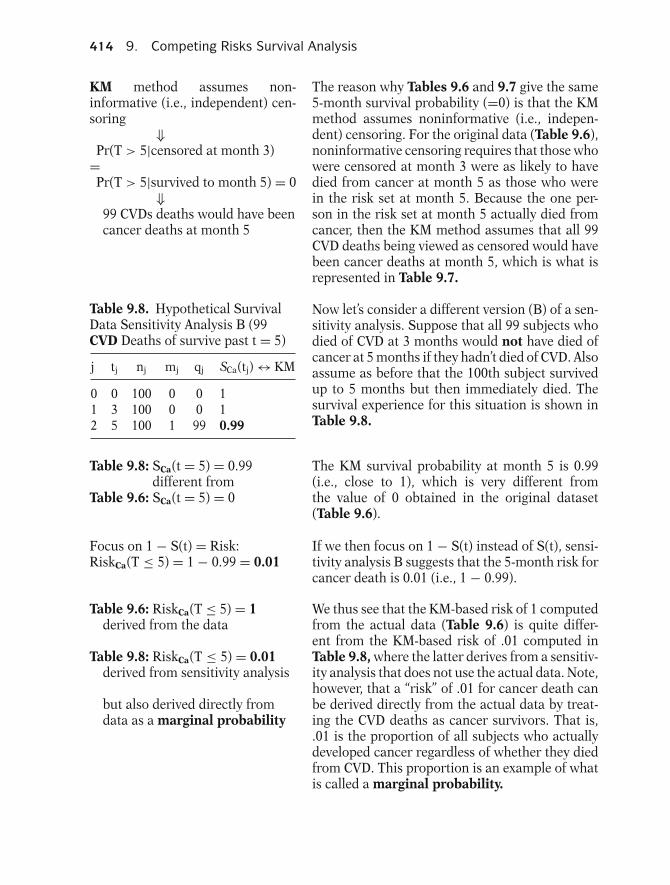
414 9. Competing Risks Survival Analysis
KM method assumes non-informative (i.e., independent) cen-soring
⇓Pr(T > 5|censored at month 3)
=Pr(T > 5|survived to month 5) = 0
⇓99 CVDs deaths would have beencancer deaths at month 5
The reason why Tables 9.6 and 9.7 give the same5-month survival probability (=0) is that the KMmethod assumes noninformative (i.e., indepen-dent) censoring. For the original data (Table 9.6),noninformative censoring requires that those whowere censored at month 3 were as likely to havedied from cancer at month 5 as those who werein the risk set at month 5. Because the one per-son in the risk set at month 5 actually died fromcancer, then the KM method assumes that all 99CVD deaths being viewed as censored would havebeen cancer deaths at month 5, which is what isrepresented in Table 9.7.
Table 9.8. Hypothetical SurvivalData Sensitivity Analysis B (99CVD Deaths of survive past t = 5)
j tj nj mj qj SCa(tj) ↔ KM
0 0 100 0 0 11 3 100 0 0 12 5 100 1 99 0.99
Now let’s consider a different version (B) of a sen-sitivity analysis. Suppose that all 99 subjects whodied of CVD at 3 months would not have died ofcancer at 5 months if they hadn’t died of CVD. Alsoassume as before that the 100th subject survivedup to 5 months but then immediately died. Thesurvival experience for this situation is shown inTable 9.8.
Table 9.8: SCa(t = 5) = 0.99different from
Table 9.6: SCa(t = 5) = 0
The KM survival probability at month 5 is 0.99(i.e., close to 1), which is very different fromthe value of 0 obtained in the original dataset(Table 9.6).
Focus on 1 − S(t) = Risk:RiskCa(T ≤ 5) = 1 − 0.99 = 0.01
If we then focus on 1 − S(t) instead of S(t), sensi-tivity analysis B suggests that the 5-month risk forcancer death is 0.01 (i.e., 1 − 0.99).
Table 9.6: RiskCa(T ≤ 5) = 1derived from the data
Table 9.8: RiskCa(T ≤ 5) = 0.01derived from sensitivity analysis
but also derived directly fromdata as a marginal probability
We thus see that the KM-based risk of 1 computedfrom the actual data (Table 9.6) is quite differ-ent from the KM-based risk of .01 computed inTable 9.8, where the latter derives from a sensitiv-ity analysis that does not use the actual data. Note,however, that a “risk” of .01 for cancer death canbe derived directly from the actual data by treat-ing the CVD deaths as cancer survivors. That is,.01 is the proportion of all subjects who actuallydeveloped cancer regardless of whether they diedfrom CVD. This proportion is an example of whatis called a marginal probability.
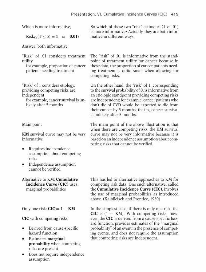
Presentation: VI. Cumulative Incidence Curves (CIC) 415
Which is more informative,
RiskCa(T ≤ 5) = 1 or 0.01?
Answer: both informative
So which of these two “risk” estimates (1 vs. 01)is more informative? Actually, they are both infor-mative in different ways.
“Risk” of .01 considers treatmentutility
for example, proportion of cancerpatients needing treatment
The “risk” of .01 is informative from the stand-point of treatment utility for cancer because inthese data, the proportion of cancer patients need-ing treatment is quite small when allowing forcompeting risks.
“Risk” of 1 considers etiology,providing competing risks areindependent
for example, cancer survival is un-likely after 5 months
On the other hand, the “risk” of 1, correspondingto the survival probability of 0, is informative froman etiologic standpoint providing competing risksare independent; for example, cancer patients whodon’t die of CVD would be expected to die fromtheir cancer by 5 months; that is, cancer survivalis unlikely after 5 months.
Main point
KM survival curve may not be veryinformative
� Requires independenceassumption about competingrisks� Independence assumptioncannot be verified
The main point of the above illustration is thatwhen there are competing risks, the KM survivalcurve may not be very informative because it isbased on an independence assumption about com-peting risks that cannot be verified.
Alternative to KM: CumulativeIncidence Curve (CIC) usesmarginal probabilities
This has led to alternative approaches to KM forcompeting risk data. One such alternative, calledthe Cumulative Incidence Curve (CIC), involvesthe use of marginal probabilities as introducedabove. (Kalbfleisch and Prentice, 1980)
Only one risk: CIC = 1 − KM
CIC with competing risks
� Derived from cause-specifichazard function� Estimates marginalprobability when competingrisks are present� Does not require independenceassumption
In the simplest case, if there is only one risk, theCIC is (1 − KM). With competing risks, how-ever, the CIC is derived from a cause-specific haz-ard function, provides estimates of the “marginalprobability” of an event in the presence of compet-ing events, and does not require the assumptionthat competing risks are independent.

416 9. Competing Risks Survival Analysis
Marginal probabilitiesUseful to assess treatment utility
in cost-effectiveness analyses
for example, 0.01 (5-month)marginal probability for Cancer(Table 9.6)
Such marginal probabilities are relevant to clini-cians in cost-effectiveness analyses in which riskprobabilities are used to assess treatment utility.For example, the .01 (5-month) marginal proba-bility for cancer derived from hypothetical datain Table 9.6 illustrates small treatment utility forcancer.
Steps to Construct CIC
1. Estimate hazard at orderedfailure times tj for event type (c)of interest
hc(tj) = mcj
nj
wheremcj = # of events for event type
c at time tjnj = # of subjects at risk at time
tj
How does one construct a CIC? We first estimatethe hazard at ordered time points tj when theevent of interest occurs. This hazard estimate issimply the number of events that occur at tj di-vided by the number at risk at tj (analogous to theKM estimate). We can write this as hc(tj) = mcj/njwhere the mcj denotes the number of events forrisk c at time tj and nj is the number of subjects atthat time. Thus, at any particular time, mcj/nj isthe estimated proportion of subjects failing fromrisk c.
2. EstimateS(tj−1) = overall survival
probability ofsurviving previoustime (tj−1)
overall ⇒ subject survivesall other competingevents
To be able to fail at time tj, the subject needs to be“around to fail”; that is, he must have survived theprevious time when a failure occurred. The prob-ability of surviving the previous time tj−1 is de-noted S(tj−1), where S(t) denotes the overall sur-vival curve rather than the cause-specific survivalcurve Sc(t). We must consider “overall” survivalhere, because the subject must have survived allother competing events.
3. Compute estimated incidence offailing from event-type c attime tj
Ic(tj) = S(tj − 1) × hc(tj)
The probability (i.e., incidence) of failing fromevent-type c at time tj is then simply the proba-bility of surviving the previous time period multi-plied by hc(tj).
4. CIC(tj) = ∑jj′=1 Ic(tj′)
= ∑jj′=1 S(tj′−1)hc(tj′)
The cumulative incidence at time tj is then the cu-mulative sum up to time tj, (i.e., from j′ = 1 toj′ = j) of these incidence values over all event-typec failure times.
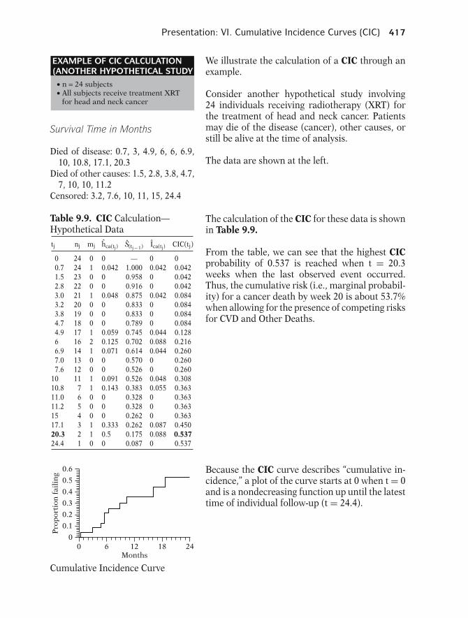
Presentation: VI. Cumulative Incidence Curves (CIC) 417
• n = 24 subjects • All subjects receive treatment XRT for head and neck cancer
EXAMPLE OF CIC CALCULATION(ANOTHER HYPOTHETICAL STUDY
We illustrate the calculation of a CIC through anexample.
Consider another hypothetical study involving24 individuals receiving radiotherapy (XRT) forthe treatment of head and neck cancer. Patientsmay die of the disease (cancer), other causes, orstill be alive at the time of analysis.
The data are shown at the left.
Survival Time in Months
Died of disease: 0.7, 3, 4.9, 6, 6, 6.9,10, 10.8, 17.1, 20.3
Died of other causes: 1.5, 2.8, 3.8, 4.7,7, 10, 10, 11.2
Censored: 3.2, 7.6, 10, 11, 15, 24.4
Table 9.9. CIC Calculation—Hypothetical Data
tj nj mj hca(tj) S(tj − 1) Ica(tj) CIC(tj)
0 24 0 0 — 0 00.7 24 1 0.042 1.000 0.042 0.0421.5 23 0 0 0.958 0 0.0422.8 22 0 0 0.916 0 0.0423.0 21 1 0.048 0.875 0.042 0.0843.2 20 0 0 0.833 0 0.0843.8 19 0 0 0.833 0 0.0844.7 18 0 0 0.789 0 0.0844.9 17 1 0.059 0.745 0.044 0.1286 16 2 0.125 0.702 0.088 0.2166.9 14 1 0.071 0.614 0.044 0.2607.0 13 0 0 0.570 0 0.2607.6 12 0 0 0.526 0 0.260
10 11 1 0.091 0.526 0.048 0.30810.8 7 1 0.143 0.383 0.055 0.36311.0 6 0 0 0.328 0 0.36311.2 5 0 0 0.328 0 0.36315 4 0 0 0.262 0 0.36317.1 3 1 0.333 0.262 0.087 0.45020.3 2 1 0.5 0.175 0.088 0.53724.4 1 0 0 0.087 0 0.537
The calculation of the CIC for these data is shownin Table 9.9.
From the table, we can see that the highest CICprobability of 0.537 is reached when t = 20.3weeks when the last observed event occurred.Thus, the cumulative risk (i.e., marginal probabil-ity) for a cancer death by week 20 is about 53.7%when allowing for the presence of competing risksfor CVD and Other Deaths.
0.6
0.5
0.4
0.3
0.2
0.1
00 6 12
Months
Pro
por
tion
fai
lin
g
18 24
Cumulative Incidence Curve
Because the CIC curve describes “cumulative in-cidence,” a plot of the curve starts at 0 when t = 0and is a nondecreasing function up until the latesttime of individual follow-up (t = 24.4).

418 9. Competing Risks Survival Analysis
CIC Summary
� Gives marginal probability� Does not use product limitformulation� Not included in mainstreamcommercially availablestatistical packages (e.g., SAS,STATA, SPSS)
Thus, as the example illustrates, the “marginalprobability” estimated by the CIC does not usea product-limit (i.e., KM) formulation. Moreover,the computation of a CIC is currently not includedin mainstream commercially available statisticalpackages.
Independence of competing risksnot required for CIC approach
As mentioned earlier, the assumption of indepen-dent competing risks is not required for the calcu-lation of the CIC, in contrast to the KM survivalcurve, which requires this assumption.
Nevertheless, CIC requires
h(t) = hc1(t) + hc2(t) + · · · + hck(t)
where
h(t) = overall hazardhc(t) = hazard for event-type c
Note: satisfied if
� Mutually exclusive event-types� Non-recurrent events
Nevertheless, the CIC does require that the overallhazard is the sum of the individual hazards forall the risk types (Kalbfleisch and Prentice, 1980).The latter assumption will be satisfied, however,whenever competing risks are mutually exclusiveand events are nonrecurrent; that is, one and onlyone event can occur at any one time and only onceover time.
Comparing CICs for 2 or moregroups:
� Statistical test available (Gray,1988)� Analogous to log rank test� No independence assumption� Does not adjust for covariates
Gray (1988) developed a test to compare twoor more CICs. This test is analogous to the logrank test. The independence assumption is notrequired. However, this test does not adjust forcovariates.
0.5
0.6
0.7
0.4
0.3
0.2
0.1
00 12 24 36 48 60
Months
Placebo, 0.2 mg DES
1.0, 5.0 mg DES
Pro
por
tion
dyi
ng
of p
rost
ate
can
cer
72
Cumulative Incidence Curves –Byar Data
The plot shown at the left gives the CICs for thetwo treatments for the Byar data.

Presentation: VI. Cumulative Incidence Curves (CIC) 419
Gray’s test results: χ2 = 6.6, df = 1p-value: 0.01
Using Gray’s test to compare the two CICs shownin the plot, we find the two curves to be signifi-cantly different (P = 0.01).
PH model used to obtain CIC⇓
Independence of competing risks re-quired
(but CIC meaningful for treatmentutility)
So far, we have described the CIC without consid-ering (Cox PH) models that account for covariates.However, when a PH model is used to obtain haz-ard ratio estimates for individual competing risksas an intermediate step in the computation of aCIC, the independence of competing risks isrequired. In any case, the CIC has a meaningfulinterpretation in terms of treatment utility regard-less of whether competing risks are independent.
Modeling CIC with covariates usingPH model: Fine and Gray (1999)
(CIC also called subdistributionfunction)
Software available (Gebski, 1997)
Fine and Gray (1999) provide methodology formodeling the CIC with covariates using a propor-tional hazards assumption. They refer to the CICcurves as subdistribution functions. The mathe-matical details of these methods are beyond thescope of this text but software is available that al-lows for such models to be fitted (Gebski, 1997)
Fine and Gray model analogous toCox PH model
Effects of predictors (e.g., HRs)have similar interpretation
The CIC models developed by Fine and Gray areanalogous to the Cox PH model but, for any fail-ure type, they model a CIC. The results from fittingthese models have a similar interpretation regard-ing the effects of predictors in the model as canbe derived from the (standard) Cox PH model ap-proach for competing risks data.
Table 9.10. Edited Output forCancer with CVD and OtherCensored—Byar Data (Fine andGray CIC Approach)Var DF Coef Std.Err. p >|z| Haz.Ratio
Rx 1 −0.414 0.171 0.008 0.661Age 1 −0.112 0.145 0.221 0.894Wt 1 0.088 0.146 0.274 1.092PF 1 0.126 0.260 0.313 1.135Hx 1 −0.256 0.182 0.080 0.774HG 1 0.321 0.191 0.046 1.379SZ 1 0.841 0.207 0.001 2.318SG 1 1.299 0.198 0.001 3.665
−2 LOG L = 1662.766546
For the Byar data, the fitted CIC model that fo-cuses on cancer deaths as the event-type of inter-est is shown in Table 9.10 below which we haverepeated Table 9.1, which uses the standard com-peting risks Cox PH model approach.
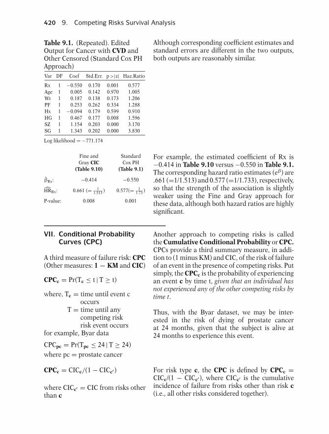
420 9. Competing Risks Survival Analysis
Table 9.1. (Repeated). EditedOutput for Cancer with CVD andOther Censored (Standard Cox PHApproach)Var DF Coef Std.Err. p >|z| Haz.Ratio
Rx 1 −0.550 0.170 0.001 0.577Age 1 0.005 0.142 0.970 1.005Wt 1 0.187 0.138 0.173 1.206PF 1 0.253 0.262 0.334 1.288Hx 1 −0.094 0.179 0.599 0.910HG 1 0.467 0.177 0.008 1.596SZ 1 1.154 0.203 0.000 3.170SG 1 1.343 0.202 0.000 3.830
Log likelihood = −771.174
Although corresponding coefficient estimates andstandard errors are different in the two outputs,both outputs are reasonably similar.
Fine and StandardGray CIC Cox PH
(Table 9.10) (Table 9.1)
βRx: −0.414 −0.550
HRRx: 0.661 (= 11.513 ) 0.577(= 1
1.73 )
P-value: 0.008 0.001
For example, the estimated coefficient of Rx is−0.414 in Table 9.10 versus −0.550 in Table 9.1.The corresponding hazard ratio estimates (eβ) are.661 (=1/1.513) and 0.577 (=1/1.733), respectively,so that the strength of the association is slightlyweaker using the Fine and Gray approach forthese data, although both hazard ratios are highlysignificant.
VII. Conditional ProbabilityCurves (CPC)
A third measure of failure risk: CPC(Other measures: 1 − KM and CIC)
CPCc = Pr(Tc ≤ t | T ≥ t)
where, Tc = time until event coccurs
T = time until anycompeting riskrisk event occurs
for example, Byar data
CPCpc = Pr(Tpc ≤ 24 | T ≥ 24)where pc = prostate cancer
Another approach to competing risks is calledthe Cumulative Conditional Probability or CPC.CPCs provide a third summary measure, in addi-tion to (1 minus KM) and CIC, of the risk of failureof an event in the presence of competing risks. Putsimply, the CPCc is the probability of experiencingan event c by time t, given that an individual hasnot experienced any of the other competing risks bytime t.
Thus, with the Byar dataset, we may be inter-ested in the risk of dying of prostate cancerat 24 months, given that the subject is alive at24 months to experience this event.
CPCc = CICc/(1 − CICc′)
where CICc′ = CIC from risks otherthan c
For risk type c, the CPC is defined by CPCc =CICc/(1 − CICc′), where CICc′ is the cumulativeincidence of failure from risks other than risk c(i.e., all other risks considered together).

Presentation: VIII. Method 2—The Lunn–McNeil (LM) Approach 421
Graphs of CPCs obtained from CICs
Tests to compare CPCs:
Pepe and Mori (1993)—2 curvesLunn (1998)—g curves
Graphs of CPC curves can be obtained from CICcurves and have been studied by Pepe–Mori (1993)and Lunn (1998). Pepe–Mori provide a test to com-pare two CPC curves. Lunn (1998) extended thistest to g-groups and allows for strata.
0.6
0.8
0.4
0.2
00 12 24 36 48 60
Months
Placebo, 0.2 mg DES
1.0, 5.0 mg DES
Pro
por
tion
dyi
ng
fro
m p
rost
ate
can
cer
72 84
Byar Data: Cumulative ConditionalProbability
For the Byar data, the plot shown here givesthe CPC curves comparing the two DES treat-ments. These curves give the probability of anevent (death) from prostate cancer at any particu-lar time given that the patient is alive at this timeto experience the event.
(Note: the Fine and Gray approach has not beenextended to model the CPCs in a regression frame-work.)
Test for equality: p-value = .01(Pepe–Mori)
The Pepe–Mori test shows a significant differencebetween these two CPC curves.
VIII. Method 2—The Lunn–McNeil (LM) Approach
Method 1: separate estimates foreach failure type, treating the com-peting failure types as censored
We have previously (Section IV) described an ap-proach (called Method 1) for analyzing competingrisks data that uses the Cox (PH) model to sep-arately estimate hazards and corresponding haz-ard ratios for each failure type, treating the other(competing) failure types as censored in additionto those not failing from any event-type.
Method 2: LM Approach
� Uses a single Cox (PH) model� Gives identical results asobtained from Method 1� Allows flexibility to performstatistical inferences notavailable from Method 1
We now describe Method 2, called the Lunn–McNeil (LM) approach, that allows only one CoxPH model to be fit rather than separate mod-els for each event-type (i.e., Method 1 above).This approach, depending on the variables put inthe model, can give identical results to those ob-tained from separate models. Moreover, the LMapproach allows flexibility to perform statisticalinferences about various features of the competingrisk models that cannot be conveniently assessedusing Method 1.
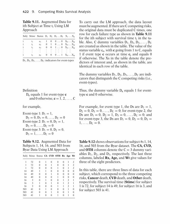
422 9. Competing Risks Survival Analysis
Table 9.11. Augmented Data forith Subject at Time ti Using LMApproach
Subj Stime Status D1 D2 D3 . . . DC X1 . . . Xp
i ti e1 1 0 0 . . . 0 Xi1 . . . Xip
i ti e2 0 1 0 . . . 0 Xi1 . . . Xip
i ti e3 0 0 1 . . . 0 Xi1 . . . Xip...
......
......
......
......
...i ti eC 0 0 0 . . . 1 Xi1 . . . Xip
D1, D2, D3, . . . , DC: indicators for event-types
To carry out the LM approach, the data layoutmust be augmented. If there are C competing risks,the original data must be duplicated C times, onerow for each failure type as shown in Table 9.11for the ith subject with survival time ti in the ta-ble. Also, C dummy variables D1, D2, D3, . . . , DCare created as shown in the table. The value of thestatus variable ec, with c going from 1 to C, equals1 if event type c occurs at time c, and equals 0if otherwise. The Xs in the table denote the pre-dictors of interest and, as shown in the table, areidentical in each row of the table.
The dummy variables D1, D2, D3, . . . ,DC are indi-cators that distinguish the C competing risks (i.e.,event-types).
DefinitionDc equals 1 for event-type c
and 0 otherwise, c = 1, 2, . . . , C
Thus, the dummy variable Dc equals 1 for event-type c and 0 otherwise.
for example,
Event-type 1: D1 = 1,D2 = 0, D3 = 0, . . . , DC = 0
Event-type 2: D1 = 0, D2 = 1,
D3 = 0, . . . , DC = 0Event-type 3: D1 = 0, D2 = 0,
D3 = 1, . . . , DC = 0
For example, for event type 1, the Ds are D1 = 1,D2 = 0, D3 = 0, . . . , DC = 0; for event-type 2, theDs are D1 = 0, D2 = 1, D3 = 0, . . . , DC = 0; andfor event-type 3, the Ds are D1 = 0, D2 = 0, D3 =1, . . . , DC = 0.
Table 9.12. Augmented Data forSubjects 1, 14, 16, and 503 fromByar Data Using LM Approach
Subj Stime Status CA CVD OTH Rx Age Wt
1 72 0 1 0 0 0 1 21 72 0 0 1 0 0 1 21 72 0 0 0 1 0 1 2
14 49 1 1 0 0 0 0 014 49 0 0 1 0 0 0 014 49 0 0 0 1 0 0 016 3 0 1 0 0 1 2 116 3 1 0 1 0 1 2 116 3 0 0 0 1 1 2 1
503 41 0 1 0 0 0 1 0503 41 0 0 1 0 0 1 0503 41 1 0 0 1 0 1 0
Table 9.12 shows observations for subject #s 1, 14,16, and 503 from the Byar dataset. The CA, CVD,and OTH columns denote the C = 3 dummy vari-ables D1, D2, and D3, respectively. The last threecolumns, labeled Rx, Age, and Wt give values forthree of the eight predictors.
In this table, there are three lines of data for eachsubject, which correspond to the three competingrisks, Cancer death, CVD death, and Other death,respectively. The survival time (Stime) for subject1 is 72, for subject 14 is 49, for subject 16 is 3, andfor subject 503 is 41.

Presentation: VIII. Method 2—The Lunn–McNeil (LM) Approach 423
From the Status and Event (i.e., CA, CVD, OTH)columns, we can see that subject 1 was censored,subject 14 died of Cancer, subject 16 died of CVD,and subject 503 died from Other causes.
For subject 1, the values for the predictors Rx, Age,and Wt, were 0, 1, and 2, respectively. These valuesappear identically in the last three columns of thethree rows for this subject. Similarly, for subject16, the predictor values for Rx, Age, and Wt, are1, 2, and 1, respectively.
General Stratified Cox LM Model
g = 1, 2, . . . , C
h∗g(t,X) = h∗
0g(t)
× exp[β1X1 + β2X2+ · · · + βpXp
+ δ21D2X1 + δ22D2X2+ · · · + δ2pD2Xp
+ δ31D3X1 + δ32D3X2+ · · · + δ3pD3Xp
+ · · ·+ δC1DCX1 + δC2DCX2+ · · · + δCpDCXp]
1st row: predictors X1, X2, . . . , Xp2nd row: product termsD2X1, D2X2, . . . , D2Xp
· · ·Cth row: product termsDCX1, DCX2, . . . , DCXp
To use the LM approach with augmented data toobtain identical results from fitting separate mod-els (Method 1), an interaction version of a strati-fied Cox PH model is required. A general form forthis model based on the notation used for the col-umn heading variables in Table 9.11 is shown atthe left.
Recall that the X1, X2, . . . , Xp denote the p predic-tors of interest. D2, D3, . . . , DC are C − 1 dummyvariables that distinguish the C event-types. Notethat event-type 1 (g = 1) is the referent group, sovariable D1 is omitted from the model. Thus, thefirst row in the exponential formula contains theXs, the second row contains product terms involv-ing D2 with each of the Xs, and so on, with the last(Cth) row containing product terms of DC witheach of the Xs. The strata (g = 1, . . . , c) are theC event-types.
LM Hazard Model forEvent-Type 1
h1(t,X) = h∗01(t)
× exp[β1X1 + β2X2+ · · · + βpXp]
(D2 = D3 = · · · = DC = 0)
For event-type 1 (g = 1), the above stratified Coxmodel simplifies to the expression shown at theleft. Note that because g = 1, the values of thedummy variables D2, D3, . . . , Dc are D2 = D3 =· · · = DC = 0.
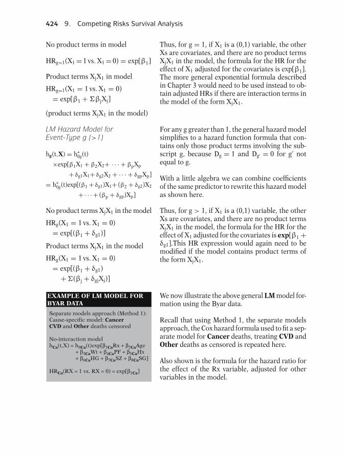
424 9. Competing Risks Survival Analysis
No product terms in model
HRg=1(X1 = 1 vs. X1 = 0) = exp[β1]
Product terms XjX1 in model
HRg=1(X1 = 1 vs. X1 = 0)= exp[β1 + �βjXj]
(product terms XjX1 in the model)
Thus, for g = 1, if X1 is a (0,1) variable, the otherXs are covariates, and there are no product termsXjX1 in the model, the formula for the HR for theeffect of X1 adjusted for the covariates is exp[β1].The more general exponential formula describedin Chapter 3 would need to be used instead to ob-tain adjusted HRs if there are interaction terms inthe model of the form XjX1.
LM Hazard Model forEvent-Type g (>1)
hg(t,X) = h∗0g(t)
×exp[β1X1 + β2X2+ · · · + βpXp
+ δg1X1+ δg2X2 + · · · + δgpXp]
= h∗0g(t)exp[(β1 + δg1)X1+ (β2 + δg2)X2
+ · · · + (βp + δgp)Xp]
For any g greater than 1, the general hazard modelsimplifies to a hazard function formula that con-tains only those product terms involving the sub-script g, because Dg = 1 and Dg′ = 0 for g′ notequal to g.
With a little algebra we can combine coefficientsof the same predictor to rewrite this hazard modelas shown here.
No product terms XjX1 in the model
HRg(X1 = 1 vs. X1 = 0)= exp[(β1 + δg1)]
Product terms XjX1 in the model
HRg(X1 = 1 vs. X1 = 0)= exp[(β1 + δg1)
+ �(βj + δgjXj)]
Thus, for g > 1, if X1 is a (0,1) variable, the otherXs are covariates, and there are no product termsXjX1 in the model, the formula for the HR for theeffect of X1 adjusted for the covariates is exp[β1 +δg1].This HR expression would again need to bemodified if the model contains product terms ofthe form XjX1.
EXAMPLE OF LM MODEL FORBYAR DATA
Separate models approach (Method 1):Cause-specific model: CancerCVD and Other deaths censored
No-interaction modelhCa(t,X) = h0Ca(t)exp[β1CaRx + β2CaAge
+ β3CaWt + β4CaPF + β5CaHx+ β6CaHG + β7CaSZ + β8CaSG]
HRCa(RX = 1 vs. RX = 0) = exp[β1Ca]
We now illustrate the above general LM model for-mation using the Byar data.
Recall that using Method 1, the separate modelsapproach, the Cox hazard formula used to fit a sep-arate model for Cancer deaths, treating CVD andOther deaths as censored is repeated here.
Also shown is the formula for the hazard ratio forthe effect of the Rx variable, adjusted for othervariables in the model.
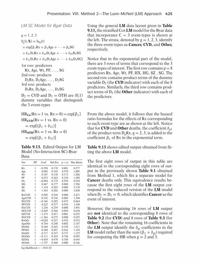
Presentation: VIII. Method 2—The Lunn–McNeil (LM) Approach 425
LM SC Model for Byar Data
g = 1, 2, 3
h∗g(t,X) = h0g(t)
× exp[β1Rx + β2Age + · · · +β8SG
+ δ21D2Rx + δ22D2Age + · · · + δ28D2SG
+ δ31D3Rx + δ32D3Age + · · · + δ38D3SG]
1st row: predictorsRx, Age, Wt, PF, . . . , SG
2nd row: productsD2Rx, D2Age, . . . , D2SG
3rd row: productsD3Rx, D2Age, . . . , D3SG
D2 = CVD and D3 = OTH are (0,1)dummy variables that distinguishthe 3 event-types
Using the general LM data layout given in Table9.11, the stratified Cox LM model for the Byar datathat incorporates C = 3 event-types is shown atthe left. The strata, denoted by g = 1, 2, 3, identifythe three event-types as Cancer, CVD, and Other,respectively.
Notice that in the exponential part of the model,there are 3 rows of terms that correspond to the 3event-types of interest. The first row contains p = 8predictors Rx, Age, Wt, PF, HX, HG, SZ , SG. Thesecond row contains product terms of the dummyvariable D2 (the CVD indicator) with each of the 8predictors. Similarly, the third row contains prod-uct terms of D3 (the Other indicator) with each ofthe predictors.
HRCa(Rx = 1 vs. Rx = 0) = exp[β1]HRCVD(Rx = 1 vs. Rx = 0)
= exp[(β1 + δ21)]HROTH(Rx = 1 vs. Rx = 0)
= exp[(β1 + δ31)]
From the above model, it follows that the hazardratio formulas for the effects of Rx correspondingto each event-type are as shown at the left. Noticethat for CVD and Other deaths, the coefficient δg1of the product term DgRx, g = 2, 3, is added to thecoefficient β1 of Rx in the exponential term.
Table 9.13. Edited Output for LMModel (No-Interaction SC)-ByarDataVar DF Coef Std.Err. p >|z| Haz.Ratio
Rx 1 −0.550 0.170 0.001 0.577Age 1 0.005 0.142 0.970 1.005Wt 1 0.187 0.138 0.173 1.206PF 1 0.253 0.262 0.334 1.288Hx 1 −0.094 0.179 0.599 0.910HG 1 0.467 0.177 0.008 1.596SZ 1 1.154 0.203 0.000 3.170SG 1 1.343 0.202 0.000 3.830
RxCVD 1 0.905 0.244 0.000 2.471AgeCVD 1 0.332 0.196 0.089 1.394WtCVD 1 −0.146 0.203 0.472 0.864PFCVD 1 0.222 0.377 0.556 1.248HxCVD 1 1.236 0.259 0.000 3.441HGCVD 1 −0.449 0.268 0.094 0.638SZCVD 1 −1.375 0.417 0.001 0.253SGCVD 1 −1.366 0.275 0.000 0.255RxOth 1 −0.028 0.327 0.932 0.972AgeOth 1 0.764 0.248 0.002 2.147WtOth 1 0.344 0.265 0.194 1.411PFOth 1 0.288 0.497 0.562 1.334HxOth 1 0.117 0.337 0.727 1.125HGOth 1 −0.111 0.345 0.748 0.895SZOth 1 −0.439 0.470 0.350 0.645SGOth 1 −1.797 0.360 0.000 0.166
log likelihood = −1831.92
Table 9.13 shows edited output obtained from fit-ting the above LM model.
The first eight rows of output in this table areidentical to the corresponding eight rows of out-put in the previously shown Table 9.1 obtainedfrom Method 1, which fits a separate model forCancer deaths only. This equivalence results be-cause the first eight rows of the LM output cor-respond to the reduced version of the LM modelwhen D2 = D3 = 0, which identifies Cancer as theevent of interest.
However, the remaining 16 rows of LM outputare not identical to the corresponding 8 rows ofTable 9.2 (for CVD) and 8 rows of Table 9.3 (forOther). Note that the remaining 16 coefficients inthe LM output identify the δgj coefficients in theLM model rather than the sum (β1 + δgj) requiredfor computing the HR when g = 2 and 3.

426 9. Competing Risks Survival Analysis
HRCa(Rx = 1 vs. Rx = 0)= exp[−0.550] = 0.577= (1/1.733)
Wald ChiSq = (−.550/.171)2
= 10.345(P = 0.001)
95% CI for exp[β1Ca]:exp[−0.550 ± 1.96(0.171)]= (0.413, 0.807)
From Table 9.13, the adjusted HR for the effect ofRx when the event-type is Cancer can be read di-rectly off the output as 0.577. Also, the Wald statis-tic for testing H0: β1 = 0 is highly significant (P =.001). The corresponding 95% confidence intervalfor this HR has the limits (0.413, 0.807).
LM results for Cancer identical toMethod 1 results for Cancer
These results are identical to those obtained forthe adjusted HR, the Wald test, and interval esti-mate obtained in Table 9.1 using Method 1 to as-sess the effect of Rx on survival for cancer death.
HRCVD(Rx = 1 vs. Rx = 0)= exp(β1 + δ11)= exp(−0.550 + 0.905)= exp(0.355) = 1.426
HROTH(Rx = 1 vs. Rx = 0)= exp(β1 + δ21)= exp(−0.550 − 0.028)= exp(−0.578) = 0.561
Using Table 9.13 to obtain adjusted HR for theRx effect when the event-type is CVD or Other,we must exponentiate the sum (β1 + δg1) for g =2 and 3, respectively.
LM results for CVD and Other iden-tical to Method 1 results for CVDand Other
These results are shown at the left, and they areidentical to those obtained in Tables 9.2 and 9.3using Method 1.
Wald test statistics for CVD andOther
WaldCVD =[
β1 + δ11
SEβ1+δ 21
]2
WaldOTH =[
β1 + δ11
SEβ1+δ 21
]2
Note, however, that using the LM model to obtainWald test statistics and 95% confidence intervalsfor the HRs for CVD and Other, the mathemat-ical formulas (shown at left for the Wald tests)require obtaining standard errors of the sums(β1 + δg1) for g = 2 and 3, whereas the output inTable 9.13 gives only individual standard errorsof β1, δ11, and δ21.
Computer packages provide forcomputation of the above formulas
SAS: test statement
STATA: lincom command
SAS and STATA provide special syntax to specifythe computer code for such computations:SAS’s PHREG allows a “test” statement; STATAallows a “lincom” command.

Presentation: IX. Method 2a—Alternative Lunn–McNeil (LMalt) Approach 427
Alternative LM formulation (LMaltmodel)
Output identical to Method 1(Tables 9.1, 9.2, 9.3)
Nevertheless, there is an alternative version of theLM model that avoids the need for special syn-tax. This alternative formulation, which we callthe LMalt model, results in output that is identicalto the output from the separate models (Method 1)approach for analyzing competing risk data asgiven in Tables 9.1 through 9.3.
IX. Method 2a—AlternativeLunn–McNeil (LMalt)Approach
� Uses same data layout asTable 9.11� Column headings:◦ Dummy variables
D1, D2, . . . , DC◦ Predictor variables
X1, X2, . . . , Xp� Above variables are transformedinto product terms
The data layout required to fit the LMalt modelis the same as shown earlier in Table 9.11. How-ever, the variables listed in the columns of this ta-ble, namely, the dummy variables D1, D2, . . . , DCand the predictor variables X1, X2, . . . , Xp, serveas basic variables that are transformed into prod-uct terms that define the LMalt model.
1st row of LMalt model:product terms
D1X1, D1X2, . . . , D1Xpcoefficients δ′
11, . . . , δ′1p
1st row of LM modelpredictors X1, X2, . . . , Xpcoefficients β1, . . . ,βp
The primary difference in the two formulasis that the first row of the exponential termin the LMalt model contains product termsD1X1, D1X2, . . . , D1Xp with coefficients denotedδ′
11, . . . , δ′1p whereas the first row in the LM
model contains the predictors X1, X2, . . . , Xpwithout product terms and coefficients denotedβ1, . . . ,βp.
General Stratified CoxLMalt Model
g = 1, . . . , C
h′g(t,X) = h′
0g(t)
× exp[δ′11D1X1 + δ′
12D1X2 + · · · + δ′1pD1Xp
+ δ′21D2X1 + δ′
22D2X2+ · · · + δ′2pD2Xp
+ δ′31D3X1 + δ′
32D3X2 + · · · + δ′3pD3Xp
+ · · ·+ δ′
C1DCX1 + δ′C2DCX2 + · · · + δ′
CpDCXp]
The general form of the LMalt model is shown atthe left. We have used a superscript prime (′) to dis-tinguish the hazard model formula for the LMaltmodel from the corresponding formula for the LMmodel given earlier.
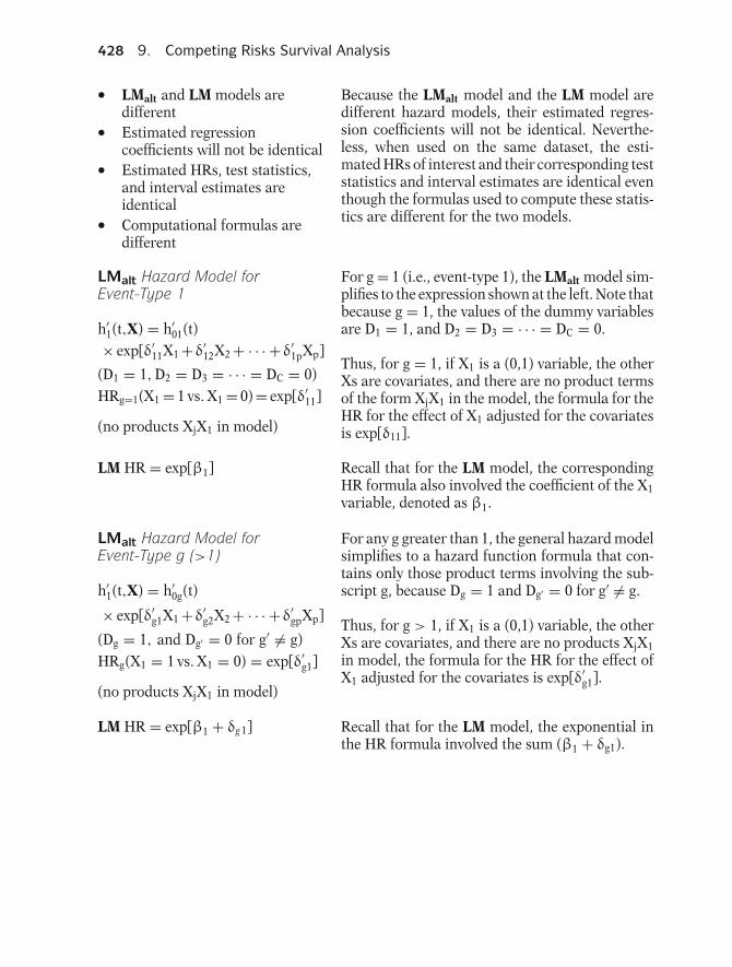
428 9. Competing Risks Survival Analysis
� LMalt and LM models aredifferent� Estimated regressioncoefficients will not be identical� Estimated HRs, test statistics,and interval estimates areidentical� Computational formulas aredifferent
Because the LMalt model and the LM model aredifferent hazard models, their estimated regres-sion coefficients will not be identical. Neverthe-less, when used on the same dataset, the esti-mated HRs of interest and their corresponding teststatistics and interval estimates are identical eventhough the formulas used to compute these statis-tics are different for the two models.
LMalt Hazard Model forEvent-Type 1
h′1(t,X) = h′
01(t)× exp[δ′
11X1 +δ′12X2 + · · · +δ′
1pXp]
(D1 = 1, D2 = D3 = · · · = DC = 0)HRg=1(X1 = 1 vs. X1 = 0) = exp[δ′
11]
(no products XjX1 in model)
For g = 1 (i.e., event-type 1), the LMalt model sim-plifies to the expression shown at the left. Note thatbecause g = 1, the values of the dummy variablesare D1 = 1, and D2 = D3 = · · · = DC = 0.
Thus, for g = 1, if X1 is a (0,1) variable, the otherXs are covariates, and there are no product termsof the form XjX1 in the model, the formula for theHR for the effect of X1 adjusted for the covariatesis exp[δ11].
LM HR = exp[β1] Recall that for the LM model, the correspondingHR formula also involved the coefficient of the X1variable, denoted as β1.
LMalt Hazard Model forEvent-Type g (>1)
h′1(t,X) = h′
0g(t)
× exp[δ′g1X1 +δ′
g2X2 + · · · +δ′gpXp]
(Dg = 1, and Dg′ = 0 for g′ �= g)HRg(X1 = 1 vs. X1 = 0) = exp[δ′
g1]
(no products XjX1 in model)
For any g greater than 1, the general hazard modelsimplifies to a hazard function formula that con-tains only those product terms involving the sub-script g, because Dg = 1 and Dg′ = 0 for g′ �= g.
Thus, for g > 1, if X1 is a (0,1) variable, the otherXs are covariates, and there are no products XjX1in model, the formula for the HR for the effect ofX1 adjusted for the covariates is exp[δ′
g1].
LM HR = exp[β1 + δg1] Recall that for the LM model, the exponential inthe HR formula involved the sum (β1 + δg1).

Presentation: IX. Method 2a—Alternative Lunn–McNeil (LMalt) Approach 429
Statistical inferences (i.e., Wald test,95% CI)
LMalt model: need standard error forδ
′g1(directly provided by output)
LM model: standard error of(β1 + δg1). (more complicatedcomputation)
Thus for g > 1, statistical inferences about HRsusing the LMalt model only require use of the stan-dard error for δ
′g1 that is directly provided in the
output.
In contrast, the LM model requires computingthe more complicated standard error of the sum(β1 + δg1).
Next: Byar data example of LMaltmodel
We now illustrate the above general LMalt modelformation using the Byar data.
LMalt SC Model for Byar Data
g = 1, 2, 3h′
g(t,X) = h0g′(t)
× exp[δ′11D1Rx + δ′
12D1Age + · · ·+ δ′
1pD1SG + δ′21D2Rx
+ δ′22D2Age + · · · + δ′
28D2SG+ δ′
31D3Rx + δ′32D3Age + · · ·
+ δ′38D3SG]
The stratified Cox (SC) LMalt model that incorpo-rates the C = 3 event-types is shown at the left.The strata, denoted by g = 1, 2, 3, identify thethree event-types, Cancer, CVD, and Other.
D1 = CA, D2 = CVD, and D3 =OTH are (0,1) dummy variables forthe 3 event-types
1st row: productsD1Rx, D1Age, . . . , D1SG(LM predictors, Rx, Age, . . . , SG)
2nd row: productsD2Rx, D2Age, . . . , D2SG
3rd row: productsD3Rx, D3Age, . . . , D3SG
Notice that in the exponential part of the model,the first row contains product terms of the dummyvariable D1 (the CA indicator) with each of the 8predictors Rx, Age, Wt, PF, HX, HG, SZ, SG. Recallthat in the LM version of this model, the first rowcontained main effects of the predictors instead ofproduct terms.
The second and third rows, as in the LM model,contain product terms of the dummy variable D2(the CVD indicator) and D3 (the OTH indicator),respectively, with each of the 8 predictors.
HRCa(Rx = 1 vs. Rx = 0) = exp[δ′11]
HRCVD(Rx = 1 vs. Rx = 0)= exp[δ′
21]HROTH(Rx = 1 vs. Rx = 0)
= exp[δ′31]
From the above model, it follows that the HR for-mulas for the effects of Rx corresponding to eachevent-type are of the form exp(δ′
g1), where δ′g1 is
the coefficient of the product term DgRx in theLMalt model.

430 9. Competing Risks Survival Analysis
Waldg =[
δ′g1
SEδ ′
g1
]2
g = 1 (CA), 2 (CVD), 3 (OTH)
Consequently, Wald test statistics (shown at theleft) and confidence intervals for these HRs usestandard errors that are directly obtained from thestandard error column from the output obtainedfor the LMalt model.
Statistical inference information
LMalt model: directly provided byoutput
LM model: not directly provided byoutput (requires additionalcomputer code)
Thus, the LMalt model allows the user to performstatistical inference procedures using the infor-mation directly provided in the computer output,whereas the LM model requires additional com-puter code to carry out more complicated compu-tations.
Table 9.14. Edited Output for SCLMalt Model—Byar Data
Var DF Coef Std.Err. p >|z| Haz.Ratio
RxCa 1 −0.550 0.170 0.001 0.577AgeCa 1 0.005 0.142 0.970 1.005WtCa 1 0.187 0.138 0.173 1.206PFCa 1 0.253 0.262 0.334 1.288HxCa 1 −0.094 0.179 0.599 0.910HGCa 1 0.467 0.177 0.008 1.596SZCa 1 1.154 0.203 0.000 3.170SGCa 1 1.343 0.202 0.000 3.830
RxCVD 1 0.354 0.174 0.042 1.429AgeCVD 1 0.337 0.134 0.012 1.401WtCVD 1 0.041 0.150 0.783 1.042PFCVD 1 0.475 0.270 0.079 1.608HxCVD 1 1.141 0.187 0.000 3.131HGCVD 1 0.018 0.202 0.929 1.018SZCVD 1 −0.222 0.364 0.542 0.801SGCVD 1 −0.023 0.186 0.900 0.977
RxOth 1 −0.578 0.279 0.038 0.561AgeOth 1 0.770 0.204 0.000 2.159WtOth 1 0.532 0.227 0.019 1.702PFOth 1 0.541 0.422 0.200 1.718HxOth 1 0.023 0.285 0.935 1.023HGOth 1 0.357 0.296 0.228 1.428SZOth 1 0.715 0.423 0.091 2.045SGOth 1 −0.454 0.298 0.127 0.635
log likelihood = −1831.916
Table 9.14 shows edited output obtained from fit-ting the above LMalt model.
The first eight rows of output in this table are iden-tical to the eight rows of output in the previouslyshown Table 9.1 obtained from Method 1, whichfits a separate model for Cancer deaths only, treat-ing CVD and Other deaths as censored.
The next eight rows in the table are identical tothe eight rows of output in the previous Table 9.2,which fits a separate model for CVD deaths only,treating Cancer and Other deaths as censored.
The last eight rows in the table are identical to theeight rows of output in the previous Table 9.3,which fits a separate model for Other deaths only,treating Cancer and CVD deaths as censored.
Table 9.14 (LMalt) outputidentical to
Tables 9.1, 9.2, 9.3 (Method 1)output combined
Thus, the output in Table 9.14 using the singleLMalt model gives identical results to what is ob-tained from fitting 3 separate models in Tables9.1, 9.2, and 9.3.
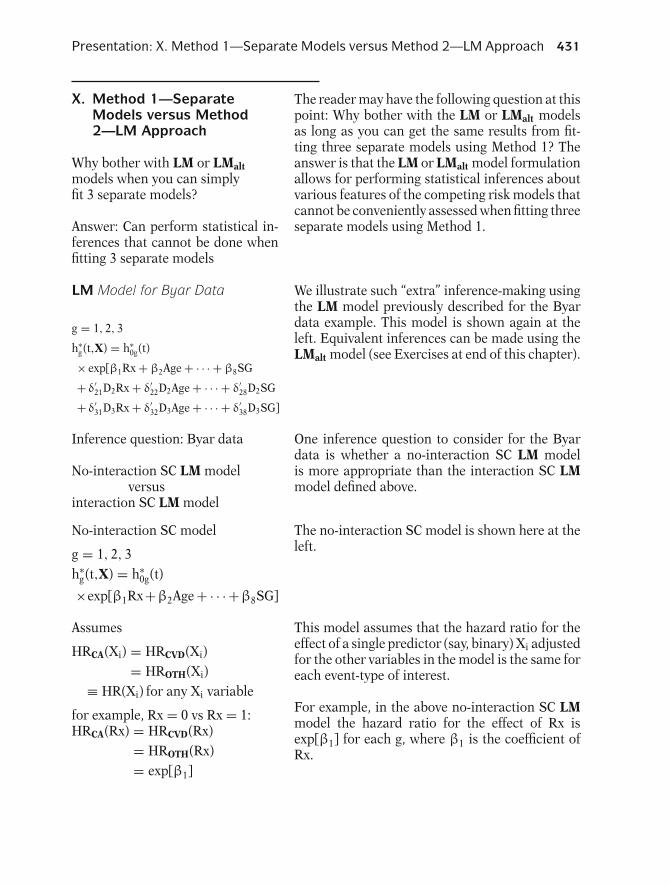
Presentation: X. Method 1—Separate Models versus Method 2—LM Approach 431
X. Method 1—SeparateModels versus Method2—LM Approach
Why bother with LM or LMaltmodels when you can simplyfit 3 separate models?
Answer: Can perform statistical in-ferences that cannot be done whenfitting 3 separate models
The reader may have the following question at thispoint: Why bother with the LM or LMalt modelsas long as you can get the same results from fit-ting three separate models using Method 1? Theanswer is that the LM or LMalt model formulationallows for performing statistical inferences aboutvarious features of the competing risk models thatcannot be conveniently assessed when fitting threeseparate models using Method 1.
LM Model for Byar Data
g = 1, 2, 3
h∗g(t,X) = h∗
0g(t)
× exp[β1Rx + β2Age + · · · + β8SG
+ δ′21D2Rx + δ′
22D2Age + · · · + δ′28D2SG
+ δ′31D3Rx + δ′
32D3Age + · · · + δ′38D3SG]
We illustrate such “extra” inference-making usingthe LM model previously described for the Byardata example. This model is shown again at theleft. Equivalent inferences can be made using theLMalt model (see Exercises at end of this chapter).
Inference question: Byar data
No-interaction SC LM modelversus
interaction SC LM model
One inference question to consider for the Byardata is whether a no-interaction SC LM modelis more appropriate than the interaction SC LMmodel defined above.
No-interaction SC model
g = 1, 2, 3h∗
g(t,X) = h∗0g(t)
×exp[β1Rx+β2Age + · · · +β8SG]
The no-interaction SC model is shown here at theleft.
Assumes
HRCA(Xi) = HRCVD(Xi)= HROTH(Xi)
≡ HR(Xi) for any Xi variable
for example, Rx = 0 vs Rx = 1:HRCA(Rx) = HRCVD(Rx)
= HROTH(Rx)= exp[β1]
This model assumes that the hazard ratio for theeffect of a single predictor (say, binary) Xi adjustedfor the other variables in the model is the same foreach event-type of interest.
For example, in the above no-interaction SC LMmodel the hazard ratio for the effect of Rx isexp[β1] for each g, where β1 is the coefficient ofRx.
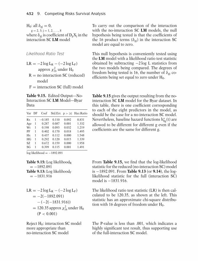
432 9. Competing Risks Survival Analysis
H0: all δgj = 0,g = 2, 3; j = 1, 2, . . . , 8
where δgj is coefficient of DgXj in theinteraction SC LM model
To carry out the comparison of the interactionwith the no-interaction SC LM models, the nullhypothesis being tested is that the coefficients ofthe 16 product terms (δgj) in the interaction SCmodel are equal to zero.
Likelihood Ratio Test
LR = −2 log LR − (−2 log LF)approx χ2
16 under H0
R = no interaction SC (reduced)model
F = interaction SC (full) model
This null hypothesis is conveniently tested usingthe LM model with a likelihood ratio test statisticobtained by subtracting −2 log L statistics fromthe two models being compared. The degrees offreedom being tested is 16, the number of δgj co-efficients being set equal to zero under H0.
Table 9.15. Edited Output—No-Interaction SC LM Model—ByarData
Var DF Coef Std.Err. p > |z| Haz.Ratio
Rx 1 −0.185 0.110 0.092 0.831Age 1 0.287 0.087 0.001 1.332Wt 1 0.198 0.093 0.032 1.219PF 1 0.402 0.170 0.018 1.495Hx 1 0.437 0.112 0.000 1.548HG 1 0.292 0.120 0.015 1.339SZ 1 0.672 0.159 0.000 1.958SG 1 0.399 0.115 0.001 1.491
log likelihood = −1892.091
Table 9.15 gives the output resulting from the no-interaction SC LM model for the Byar dataset. Inthis table, there is one coefficient correspondingto each of the eight predictors in the model, asshould be the case for a no-interaction SC model.Nevertheless, baseline hazard functions h∗
0g(t) areallowed to be different for different g even if thecoefficients are the same for different g.
Table 9.15: Log likelihoodR
= −1892.091Table 9.13: Log likelihoodF
= −1831.916
From Table 9.15, we find that the log-likelihoodstatistic for the reduced (no-interaction SC) modelis −1892.091. From Table 9.13 (or 9.14), the log-likelihood statistic for the full (interaction SC)model is −1831.916.
LR = −2 log LR − (−2 log LF)= −2(−1892.091)
− (−2(−1831.916))= 120.35 approx χ2
16 under H0
(P < 0.001)
The likelihood ratio test statistic (LR) is then cal-culated to be 120.35, as shown at the left. Thisstatistic has an approximate chi-square distribu-tion with 16 degrees of freedom under H0.
Reject H0: interaction SC modelmore appropriate thanno-interaction SC model
The P-value is less than .001, which indicates ahighly significant test result, thus supporting useof the full-interaction SC model.
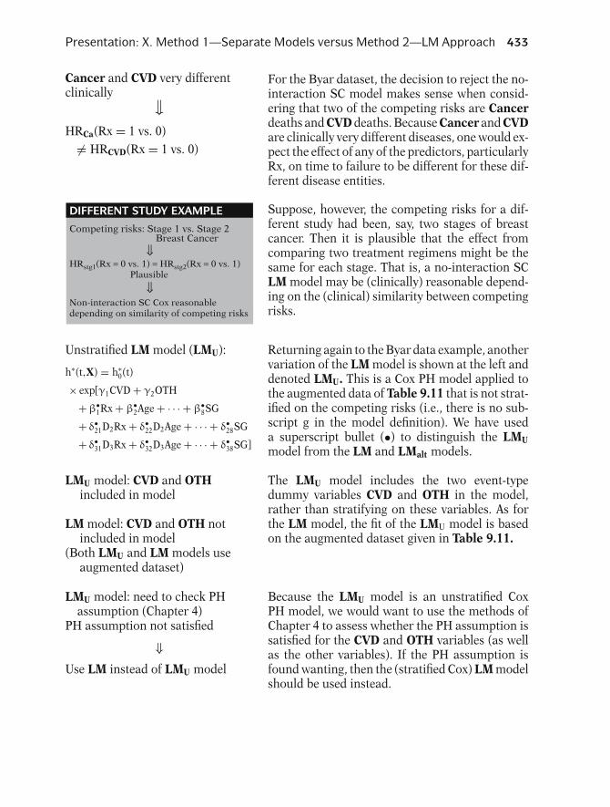
Presentation: X. Method 1—Separate Models versus Method 2—LM Approach 433
Cancer and CVD very differentclinically ,-HRCa(Rx = 1 vs. 0)
�= HRCVD(Rx = 1 vs. 0)
For the Byar dataset, the decision to reject the no-interaction SC model makes sense when consid-ering that two of the competing risks are Cancerdeaths and CVD deaths. Because Cancer and CVDare clinically very different diseases, one would ex-pect the effect of any of the predictors, particularlyRx, on time to failure to be different for these dif-ferent disease entities.
DIFFERENT STUDY EXAMPLE
⇓
⇓
Competing risks: Stage 1 vs. Stage 2Breast Cancer
HRstg1(Rx = 0 vs. 1) = HRstg2(Rx = 0 vs. 1) Plausible
Non-interaction SC Cox reasonabledepending on similarity of competing risks
Suppose, however, the competing risks for a dif-ferent study had been, say, two stages of breastcancer. Then it is plausible that the effect fromcomparing two treatment regimens might be thesame for each stage. That is, a no-interaction SCLM model may be (clinically) reasonable depend-ing on the (clinical) similarity between competingrisks.
Unstratified LM model (LMU):
h∗(t,X) = h∗0(t)
× exp[γ1CVD + γ2OTH
+β•1Rx + β•
2Age + · · · + β•8SG
+ δ•21D2Rx + δ•
22D2Age + · · · + δ•28SG
+ δ•31D3Rx + δ•
32D3Age + · · · + δ•38SG]
Returning again to the Byar data example, anothervariation of the LM model is shown at the left anddenoted LMU. This is a Cox PH model applied tothe augmented data of Table 9.11 that is not strat-ified on the competing risks (i.e., there is no sub-script g in the model definition). We have useda superscript bullet (•) to distinguish the LMUmodel from the LM and LMalt models.
LMU model: CVD and OTHincluded in model
LM model: CVD and OTH notincluded in model
(Both LMU and LM models useaugmented dataset)
The LMU model includes the two event-typedummy variables CVD and OTH in the model,rather than stratifying on these variables. As forthe LM model, the fit of the LMU model is basedon the augmented dataset given in Table 9.11.
LMU model: need to check PHassumption (Chapter 4)
PH assumption not satisfied
⇓Use LM instead of LMU model
Because the LMU model is an unstratified CoxPH model, we would want to use the methods ofChapter 4 to assess whether the PH assumption issatisfied for the CVD and OTH variables (as wellas the other variables). If the PH assumption isfound wanting, then the (stratified Cox) LM modelshould be used instead.

434 9. Competing Risks Survival Analysis
PH assumption satisfied⇓
Determine HRs using exponentialformula (Chapter 3)
If the PH assumption is satisfied, hazard ratios forthe effects of various predictors in the LMU modelcan be determined using the standard exponentialformula described in Chapter 3 for the Cox PHmodel.
Cancer survival (CVD = OTH = 0):
HRCa(Rx = 1 vs. Rx = 0) = exp[δ•11]
CVD survival (CVD = 1, OTH = 0):
HRCVD(Rx = 1 vs. Rx = 0)= exp[γ1 + δ•
21]
Other survival (CVD = 0, OTH = 1):
HROTH(Rx = 1 vs. Rx = 0)= exp[γ1 + δ•
31]
In particular, to obtain the hazard ratio for the ef-fect of Rx on Cancer survival, we would specifyCVD = OTH = 0 in the model and then exponen-tiate the coefficient of the Rx variable in the model,as shown at the left.
Similar HR expressions (but involving γ1 and γ2also) are obtained for the effect of Rx when CVDdeaths and Other deaths are the event-types ofinterest.
Essential point
Use of single LM-type model offersgreater flexibility for the analysisthan allowed using Method 1
At this point, we omit further description of re-sults from fitting the LMU model to the Byardataset. The essential point here is that the useof a single LM-type model with augmented dataallows greater flexibility for the analysis than canbe achieved when using Method 1 to fit separatehazard models for each event-type of interest.
XI. Summary
Competing Risks
Each subject can experience onlyone of several different types ofevents over follow-up
This chapter has considered survival data in whicheach subject can experience only one of several dif-ferent types of events over follow-up. The differentevents are called competing risks.
Typical approach
� Cox PH model� Separate model for eachevent-type� Other (competing) event-typestreated as censored
We have described how to model competing riskssurvival data using a Cox PH model. The typicalapproach for analyzing competing risks data isto perform a survival analysis for each event-typeseparately, where the other (competing) event-types are treated as censored categories.
Presentation: XI. Summary 435
Drawbacks
1. Require independent competingrisks that is, censored subjectshave same risk as all subjects inrisk set
2. Product-limit (e.g., KM) curvehas questionable interpretation
There are two primary drawbacks to the abovemethod. One problem is the requirement thatcompeting risks be independent. This assumptionwill not be satisfied if those subjects censored fromcompeting risks do not have the same risk for fail-ing as subjects who are not censored from thecause-specific event of interest at that same time.
A second drawback is that the estimated product-limit survival curve obtained from fitting separateCox models for each event-type has questionableinterpretation when there are competing risks.
Several alternative strategies re-garding independence assumption:No single strategy is always best
Regarding the independence assumption, severalalternative strategies for addressing this issue aredescribed, although no single strategy is alwaysbest.
Sensitivity analysis: worst-case vio-lations of independence assumption
For example, subjects censoredfrom competing risks treated inanalysis as if
� All event-free� All experience event of interest
A popular strategy is a sensitivity analysis, whichallows the estimation of parameters by consider-ing worst-case violations of the independence as-sumption. For example, subjects censored fromcompeting risks might be treated in the analysisas either all being event-free or all experiencingthe event of interest.
� Independence assumption noteasily verifiable� Typical analysis assumesindependence assumption issatisfied
Unfortunately, the independence assumption isnot easily verifiable. Consequently, the typicalcompeting risks analysis assumes that the inde-pendence assumption is satisfied even if this is notthe case.
CIC Alternative to KM
� Derived from cause-specifichazard function� Estimates marginalprobability when competingrisks are present� Does not require independenceassumption� Useful to assess treatment utilityin cost-effectiveness analyses
To avoid a questionable interpretation of the KMsurvival curve, the primary alternative to usingKM is the Cumulative Incidence Curve (CIC),which estimates the marginal probability of anevent. Marginal probabilities are relevant for as-sessing treatment utility whether competing risksare independent.
436 9. Competing Risks Survival Analysis
CIC(tj) =j∑
j′=1
Ic(tj′)
=j∑
j′=1
S(tj′−1)hc(tj′)
hc(tj′) = estimated hazard at orderedfailure time tj′ for the event-type (c)
S(tj′−1) = overall survival probabil-ity of previous time (tj′−1)
The formula for the calculating the CIC is shownat the left. The hc(tj′) in the formula is the esti-mated hazard at survival time tj′ for the event-type (c) of interest. The term S(tj′−1) denotesthe overall survival probability of previous time(tj′−1), where “overall survival” indicates a subjectthat survives all competing events.
CIC
� Does not use product limitformulation� Not included in mainstreamcommercially availablestatistical packages (e.g., SAS,STATA, SPSS)
As the formula indicates, the CIC is not estimatedusing a product-limit formulation. Also, its com-putation is not included in mainstream commer-cially available standard statistical packages.
PH model used to obtain CIC⇓
Independence of competing risks re-quired
If a proportional hazard model is used to obtainhazard ratio estimates for individual competingrisks as an intermediate step in the computation ofa CIC, the assumption of independent competingrisks is still required.
Modeling CIC with covariates usingPH model: Fine and Gray (1999)
Software available (Gebski, 1997)Fine and Gray model analogous toCox PH model
Recent work of Fine and Gray (1999) providesmethodology for modeling the CIC with covariatesusing a proportional hazards assumption. Soft-ware is available for this method (Gebski, 1997,Tai et al., 2001), although not in standard com-mercial packages.
Alternative to CIC
CPCc = Pr(Tc ≤ t | T ≥ t)
where Tc = time until event coccurs
T = time until anycompeting risk eventoccurs
An alternative to the CIC is the Conditional Prob-ability Curve (CPC). For risk type c, CPCc is theprobability of experiencing an event c by time t,given that an individual has not experienced any ofthe other competing risks by time t.
CPCc = CICc/(1 − CICc′)
where CICc′ = CIC from risks otherthan c
The CPC can be computed from the CIC throughthe formula CPCc = CICc/(1 − CICc′), where CICc′
is the cumulative incidence of failure from risksother than risk c (i.e., all other risks consideredtogether).
Presentation: XI. Summary 437
Tests to compare CPCs:
Pepe and Mori (1993)—2 curvesLunn (1998)—g curves
Pepe–Mori provide a test to compare two CPCcurves. Lunn (1998) extended this test to g-groupsand allows for strata.
Method 2: LM Approach
� Uses a single Cox (PH) model� Gives identical results asobtained from Method 1� Allows flexibility to performstatistical inferences notavailable from Method 1
We have also described an alternative approach,called the Lunn–McNeil (LM) approach, for an-alyzing competing risks data. The LM approachallows only one model to be fit rather than sep-arate models for each event-type (Method 1).This method is equivalent to using Method 1.The LM model also allows the flexibility to per-form statistical inferences to determine whethera simpler version of an initial LM model is moreappropriate.
Augmented Data for ith Subject atTime t Using LM Approach
Subj Stime Status D1 D2 D3 . . . DC X1 . . . Xp
i ti e1 1 0 0 . . . 0 Xi1 . . . Xip
i ti e2 0 1 0 . . . 0 Xi1 . . . Xip
i ti e3 0 0 1 . . . 0 Xi1 . . . Xip
......
......
......
......
......
i ti eC 0 0 0 . . . 1 Xi1 . . . Xip
To carry out the LM approach, the data layoutmust be augmented. If there are C competing risks,the original data must be duplicated C times, onerow for each failure type.
g = 1, 2, . . . , C
h∗g(t,X) = h∗
0g(t)
× exp[β1X1 + β2X2 + · · · + βpXp
+ δ21D2X1 + δ22D2X2 + · · · + δ2pD2Xp
+ δ31D3X1 + δ32D3X2 + · · · + δ3pD3Xp
+ · · ·+ δC1DCX1 + δC2DCX2 + · · · + δCpDCXp]
To use the LM approach with augmented data toobtain identical results from fitting separate mod-els (Method 1), an interaction version of a strati-fied Cox (SC) PH model is required. A general formfor this model is shown at the left.
LM model: need standard error of
(β1 + δg1)
(special syntax required for compu-tation)
The LM model can be used to obtain Wald teststatistics and 95% confidence intervals for HRsseparately for each competing risk. These statis-tics require obtaining standard errors of the sumsof estimated regression coefficients (e.g., β1 +δg1). Such computations require special syntaxavailable in standard computer packages such asSAS, STATA, and SPSS.

438 9. Competing Risks Survival Analysis
Alternative LM formulation: LMaltmodel
LMalt yields output identical toMethod 1
Nevertheless, there is an alternative formation ofthe LM model that avoids the need for special syn-tax. This alternative formulation, called the LMaltmodel, yields output that is identical to the outputfrom the separate models (Method 1) approach foranalyzing competing risk data.
1st row of LMalt model
Product terms D1X1, D1X2, . . . , D1Xp
Coefficients δ′11,. . . ,δ
′1p
1st row of LM model
Predictors X1, X2, . . . , Xp
Coefficients β1, . . . ,βp
The primary difference in the two formulasis that the first row of the exponential termin the LMalt model contains product termsD1X1, D1X2, . . . , D1Xp1 with coefficients denotedδ′
11, . . . , δ′1p whereas the first row in the LM
model contains the predictors X1, X2, . . . , Xpwithout product terms and coefficients denotedβ1, . . . ,βp.
LMalt model: Waldg =[
δ′g1
SEδ ′
g1
]2
directly obtained from output
Using the LMalt model, Wald test statistics (shownat the left) and confidence intervals use standarderrors that are directly obtained from the stan-dard error column from the output obtained forthe LMalt model.
Statistical inference information
LMalt model: directly provided byoutput
LM model: not directly provided byoutput (requires additionalcomputer code)
Thus, the LMalt model allows the user to performstatistical inference procedures using the infor-mation directly provided in the computer output,whereas the LM model requires additional com-puter code to carry out more complicated compu-tations.
Advantage of LM (Method 2) overmethod 1:
LM offers flexibility for statisticalinferences to consider simplermodels
An advantage of using either the LM or LMalt ap-proach instead of fitting separate models (Method1) is the flexibility to perform statistical inferencesthat consider simpler versions of an interaction SCLM model.

Presentation: XI. Summary 439
For example,No-interaction SC LM model
versusinteraction SC LM model
Unstratified LM modelversus
SC LM model
For example, one inference question to consider iswhether a no-interaction SC LM model is more ap-propriate than an interaction SC model. A differ-ent question is whether an unstratified LM modelis more appropriate than a stratified LM model.These questions can be conveniently addressed us-ing a single ( i.e., LM) model instead of fitting sep-arate models (Method 1).
Overall,
� Can use standard computerpackages� Independence assumptionrequired
Overall, in this chapter, we have shown that com-peting risks data can be analyzed using standardcomputer packages provided it can be assumedthat competing risks are independent.
440 9. Competing Risks Survival Analysis
DetailedOutline
I. Overview (page 396)A. Focus: competing risks—analysis of survival data
in which each subject can experience only one ofdifferent types of events over follow-up.
B. Analysis using Cox PH model.C. Drawbacks to typical approach that uses Cox
model.D. Alternative approaches for analysis.
II. Examples of Competing Risks Data(pages 396–398)A. Dying from either lung cancer or stroke.
1. Assess whether lung cancer death rate inexposed” persons is different from lung cancerdeath rate in “unexposed,” allowing forcompeting risks.
2. Also, compare lung cancer with stroke deathrates controlling for predictors.
B. Advanced cancer patients either dying fromsurgery or getting hospital infection.1. If focus on hospital infection failure, then
death from surgery reduces burden of hospitalinfection control required.
C. Soldiers dying in accident or in combat.1. Focus on combat deaths.2. If entire company dies from accident on way to
combat, then KM survival probability forcombat death is undefined.
3. Example illustrates that interpretation of KMcurve may be questionable when there arecompeting risks.
D. Limb sarcoma patients developing localrecurrence, lung metastasis, or other metastasis.1. None of failure types involves death, so
recurrent events are possible.2. Can avoid problem of recurrent events if focus
only on time to first failure.3. Analysis of recurrent events and competing
risks in same data not addressed.III. Byar Data (pages 399–400)
A. Randomized clinical trial comparing treatmentsfor prostate cancer.
B. Three competing risks: deaths from prostatecancer, CVD, or other causes.

Detailed Outline 441
C. Covariates other than treatment are Age, Weight(Wt), Performance Status (PF), History of CVD(Hx), Hemoglobin (Hg), Lesion size (SZ), andGleeson score (SG).
D. Competing risks considered independent, forexample, death from CVD independent of deathfrom death from cancer.
IV. Method 1—Separate Models for Different EventTypes (pages 400–403)A. Use Cox (PH) model to estimate separate hazards
and HRs for each failure type, where othercompeting risks are treated as censored in additionto usual reasons for censoring: loss to follow-up,withdrawal from study, or end of study.
B. Cause-specific hazard function:hc(t) = lim�t→0 P(t ≤ Tc < t + �t|Tc ≥ t)/�twhere Tc = time-to-failure from event c, c = 1,2,. . ., C (# of event types).
C. Cox PH cause-specific model (event-type c):
hc(t,X) = h0c(t)exp[p∑
i=1
βicXi]
where c = 1, . . . , C, and βic allows effect of Xi todiffer by event-type.
D. Byar data example: Cancer, CVD, Other Deaths areC = 3 competing risks.1. Cause-specific (no-interaction) model for
Cancer:
hCa(t,X) = h0Ca(t) exp[β1CaRx + β2CaAge+β3CaWt + β4CaPF + β5CaHx+β6CaHG + β7CaSZ + β8CaSG]
where CVD and Other deaths treated ascensored observations
HRCa(RX = 1 vs. RX = 0) = exp[β1Ca]
2. Separate cause-specific (no-interaction) modelsfor CVD and Other.
3. Edited output presented for each cause-specificmodel:a. Cause-specific Cancer results for RX (with
CVD and Other censored):
HRCa(RX = 1 vs. RX = 0) = 0.575 (P = 0.001)

442 9. Competing Risks Survival Analysis
b. Cause-specific CVD results for RX (withCancer and Other censored):
HRCVD(RX = 1 vs. RX = 0) = 1.429 (P = 0.040)
c. Cause-specific Other results for RX (withCancer and CVD censored):
HROTH(RX= 1 vs. RX = 0) = 0.560 (P = 0.038)
V. The Independence Assumption (pages 403–411)A. Non-informative (independent) censoring: risk
for being censored at time t does not depend onprognosis for failure at time t.1. Typical context: no competing risks;
homogeneous sample.2. Informative censoring can lead to bias results.
B. Non-informative (independent) censoring withcompeting risks. Any subject in the risk set attime t with a given set of covariates is just as likelyto be censored at time t as any other subject in therisk set with the same set of covariates regardlessof whether the reason for censoring is a competingrisk, withdrawal from study, or loss to follow-up.1. Informative censoring: subject in risk set at
time t is more likely to be censored from acompeting risk than other subjects in the riskset at the same time.
2. Homogeneous: subjects in the risk set havingthe same values of the predictors of interest.
3. Synonym: Competing risks are independent.C. Assessing the independence assumption.
1. No method available to directly assess theindependence assumption nor guaranteeunbiased estimates if independenceassumption is violated.
2. Consequently, the typical analysis of competingrisks assumes that the independenceassumption is satisfied, even if not.
3. Strategies for considering independenceassumptiona. Decide that assumption holds on clinical/
biological/other grounds.b. Include in your model variables that are
common risk factors for competing risks.
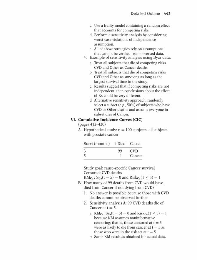
Detailed Outline 443
c. Use a frailty model containing a random effectthat accounts for competing risks.
d. Perform a sensitivity analysis by consideringworst-case violations of independenceassumption.
e. All of above strategies rely on assumptionsthat cannot be verified from observed data.
4. Example of sensitivity analysis using Byar data.a. Treat all subjects that die of competing risks
CVD and Other as Cancer deaths.b. Treat all subjects that die of competing risks
CVD and Other as surviving as long as thelargest survival time in the study.
c. Results suggest that if competing risks are notindependent, then conclusions about the effectof Rx could be very different.
d. Alternative sensitivity approach: randomlyselect a subset (e.g., 50%) of subjects who haveCVD or Other deaths and assume everyone insubset dies of Cancer.
VI. Cumulative Incidence Curves (CIC)(pages 412–420)A. Hypothetical study: n = 100 subjects, all subjects
with prostate cancer
Survt (months) # Died Cause
3 99 CVD5 1 Cancer
Study goal: cause-specific Cancer survivalCensored: CVD deathsKMCa : SCa(t = 5) = 0 and RiskCa(T ≤ 5) = 1
B. How many of 99 deaths from CVD would havedied from Cancer if not dying from CVD?1. No answer is possible because those with CVD
deaths cannot be observed further.2. Sensitivity analysis A: 99 CVD deaths die of
Cancer at t = 5.a. KMCa: SCa(t = 5) = 0 and RiskCa(T ≤ 5) = 1
because KM assumes noninformativecensoring; that is, those censored at t = 3were as likely to die from cancer at t = 5 asthose who were in the risk set at t = 5.
b. Same KM result as obtained for actual data.
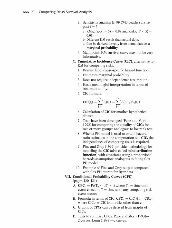
444 9. Competing Risks Survival Analysis
3. Sensitivity analysis B: 99 CVD deaths survivepast t = 5.a. KMCa: SCa(t = 5) = 0.99 and RiskCa(T ≤ 5) =
0.01.b. Different KM result than actual data.c. Can be derived directly from actual data as a
marginal probability.4. Main point: KM survival curve may not be very
informative.C. Cumulative Incidence Curve (CIC): alternative to
KM for competing risks.1. Derived from cause-specific hazard function.2. Estimates marginal probability.3. Does not require independence assumption.4. Has a meaningful interpretation in terms of
treatment utility.5. CIC formula:
CIC(tj) =j∑
j′=1
Ic(tj′) =j∑
j′=1
S(tj′−1)hc(tj′)
6. Calculation of CIC for another hypotheticaldataset.
7. Tests have been developed (Pepe and Mori,1992) for comparing the equality of CICs fortwo or more groups: analogous to log rank test.
8. When a PH model is used to obtain hazardratio estimates in the computation of a CIC, theindependence of competing risks is required.
9. Fine and Gray (1999) provide methodology formodeling the CIC (also called subdistributionfunction) with covariates using a proportionalhazards assumption: analogous to fitting CoxPH model.
10. Example of Fine and Gray output comparedwith Cox PH output for Byar data.
VII. Conditional Probability Curves (CPC)(pages 420–421)A. CPCc = Pr(Tc ≤ t|T ≥ t) where Tc = time until
event c occurs, T = time until any competing riskevent occurs.
B. Formula in terms of CIC: CPCc = CICc/(1 − CICc′)where CICc′ = CIC from risks other than c.
C. Graphs of CPCs can be derived from graphs ofCICs.
D. Tests to compare CPCs: Pepe and Mori (1993)—2 curves; Lunn (1998)—g curves.

Detailed Outline 445
VIII. Method 2—Lunn–McNeil (LM) Approach(pages 421–427)A. Allows only one Cox PH model to be fit rather than
fitting separate modes for each event type(Method 1).
B. LM uses an augmented data layout.1. For ith subject at time ti, layout has C rows of
data, where C = # event-types.2. Dummy variables D1, D2, . . . , DC are created to
distinguish the C event-types.3. The Status variable, ec, c = 1, . . . , C, equals 1
for event-type c and 0 otherwise.4. Predictors are denoted by X1, . . . , Xp.5. Example of data layout for Byar dataset.
C. General form of LM model (interaction SC model).
h∗g(t,X)
g = 1,2,...,C
= h∗0g(t) exp[β1X1 + β2X2 + · · · + βpXp
+ δ21D2X1 + δ22D2X2 + · · · + δ2pD2Xp
+ δ31D3X1 + δ32D3X2 + · · · + δ3pD3Xp
+ · · ·+ δC1DCX1 +δC2DCX2 +· · ·+δCpDCXp]
1. LM model for event-type g = 1:a. h∗
1(t,X) = h∗01(t)
× exp[β1X1 + β2X2 + · · · + βpXp]b. D2 = D3 = · · · = DC = 0c. HRg=1(X1 = 1 vs. X1 = 0) = exp[β1]
2. LM model for event-type g (>1):a. h∗
g(t,X) = h∗0g(t)
× exp[(β1 + δg1)X1 + (β2 + δg2)X2
+ · · · + (βp + δgp)Xp]b. HRg(X1 = 1 vs. X1 = 0 = exp[(β1 + δg1)]
D. LM model for Byar data.1. h∗
g(t,X) = h∗0g(t)
× exp[β1Rx + β2Age + · · · + β8SG+ δ21D2Rx + δ22D2Age + · · · + δ28D2SG+ δ31D3Rx + δ32D3Age + · · · + δ38D3SG]
g = 1, 2, 32. D2 = CVD and D3 = OTH are (0,1) dummy
variables for 3 event-types.

446 9. Competing Risks Survival Analysis
3. HRCa(Rx = 1 vs. Rx = 0) = exp[β1]HRCVD(Rx = 1 vs. Rx = 0) = exp[β1 + δ21]HROTH(Rx = 1 vs. Rx = 0) = exp[β1 + δ31]
4. Mathematical formulas for Wald tests andconfidence intervals require standard errors forsums (β1 + δg1) for g = 2 and 3; requiresspecial syntax for computer.
5. Output provided and compared to output fromMethod 1.
IX. Method 2a—Alternative Lunn–McNeil (LMalt)Approach (pages 427–430)A. An alternative LM formulation that gives identical
output to that obtained from Method 1 (separatemodels approach).
B. Same data layout as for LM model, but onlyproduct terms in LMalt model.
C. General form of LMalt (interaction SC) model:
g = 1, . . . , Ch′
g(t,X) = h0g′(t)
× exp[δ′11D1X1 + δ′
12D1X2 + · · · + δ′1pD1Xp
+ δ′21D2X1 + δ′
22D2X2 + · · · + δ′2pD2Xp
+ · · ·+ δ′
C1DCX1 + δ′C2DCX2 + · · · + δ′
CpDCXp]
D. Hazard ratio formula involves only coefficients ofproduct terms for all g:
HRg(X1 = 1 vs. X1 = 0) = exp[δ′g1], g = 1, 2, 3
a. Statistical inference information directly providedby LMalt output.
E. Example of output for LMalt model using Byardata.
X. Method 1—Separate Models versus Method 2—LMApproach (pages 431–434)A. LM and LMalt models allow flexibility to perform
statistical inferences about features of competingrisks model not conveniently available usingseparate models (Method 1) approach.
B. LM and LMalt models can assess whether ano-interaction SC model is more appropriate thanthe initial interaction SC LM model.

Practice Exercises 447
C. Example of comparison of no-interaction withinteraction SC model using Byar data.
D. LM and LMalt models can assess whether anunstratified LM model (called LMU) is moreappropriate than a stratified LM model.
E. Example of LMU model involving Byar data.XI. Summary (pages 434–439)
A. Competing risks survival data can be analyzedusing Cox PH models and standard computerpackages.
B. There are two alternative methods that use a CoxPH model formulation.1. Fit separate models for each cause-specific
event type, treating the remaining event typesas censored.
2. Use the Lunn–McNeil (LM) approach to fit asingle model that incorporates the analysis foreach cause-specific event.
C. Each of the above approaches requires thatcompeting risks be independent (noninformativecensoring).
D. Without the independence assumption, methodsfor competing risks analysis are unavailable.
E. The Cumulative Incidence Curve (CIC) or theConditional Probability Curve (CPC) arealternatives to the KM curve, when use of a KMcurve has questionable interpretation.
PracticeExercises
Answer questions 1 to 15 as true or false (circle T or F).
T F 1. A competing risk is an event-type (i.e., failure sta-tus) that can occur simultaneously with anotherevent of interest on the same subject.
T F 2. An example of competing risks survival data is astudy in which patients receiving radiotherapy forhead and neck cancer may either die from theircancer or from some other cause of death.
T F 3. If all competing risks in a given study are differentcauses of death, then it is possible to have bothcompeting risks and recurrent events in the samestudy.
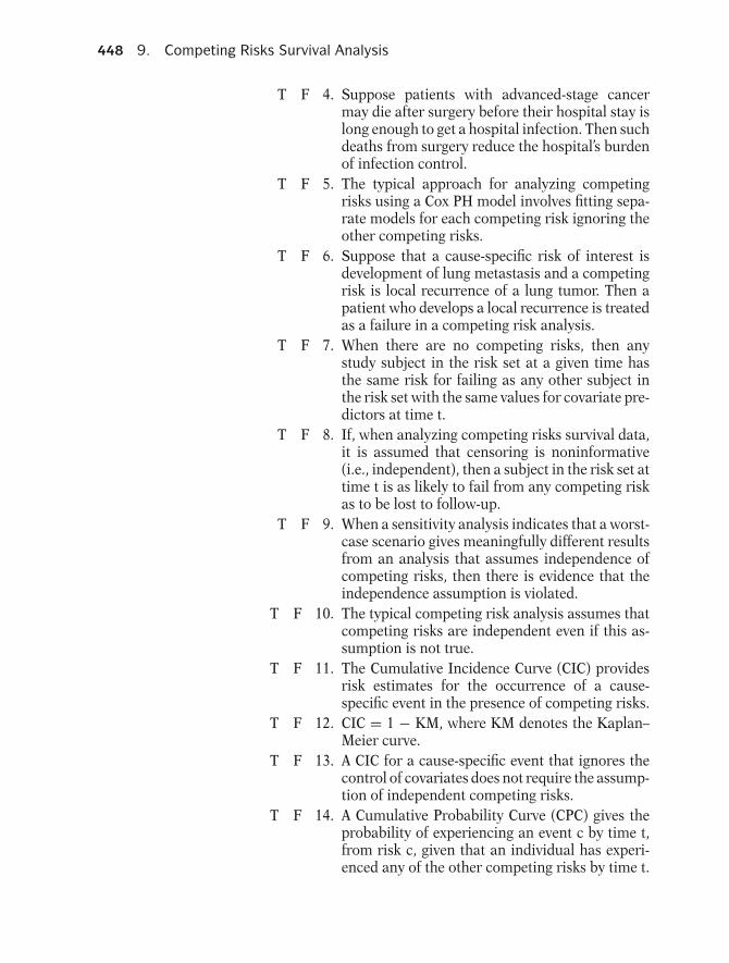
448 9. Competing Risks Survival Analysis
T F 4. Suppose patients with advanced-stage cancermay die after surgery before their hospital stay islong enough to get a hospital infection. Then suchdeaths from surgery reduce the hospital’s burdenof infection control.
T F 5. The typical approach for analyzing competingrisks using a Cox PH model involves fitting sepa-rate models for each competing risk ignoring theother competing risks.
T F 6. Suppose that a cause-specific risk of interest isdevelopment of lung metastasis and a competingrisk is local recurrence of a lung tumor. Then apatient who develops a local recurrence is treatedas a failure in a competing risk analysis.
T F 7. When there are no competing risks, then anystudy subject in the risk set at a given time hasthe same risk for failing as any other subject inthe risk set with the same values for covariate pre-dictors at time t.
T F 8. If, when analyzing competing risks survival data,it is assumed that censoring is noninformative(i.e., independent), then a subject in the risk set attime t is as likely to fail from any competing riskas to be lost to follow-up.
T F 9. When a sensitivity analysis indicates that a worst-case scenario gives meaningfully different resultsfrom an analysis that assumes independence ofcompeting risks, then there is evidence that theindependence assumption is violated.
T F 10. The typical competing risk analysis assumes thatcompeting risks are independent even if this as-sumption is not true.
T F 11. The Cumulative Incidence Curve (CIC) providesrisk estimates for the occurrence of a cause-specific event in the presence of competing risks.
T F 12. CIC = 1 − KM, where KM denotes the Kaplan–Meier curve.
T F 13. A CIC for a cause-specific event that ignores thecontrol of covariates does not require the assump-tion of independent competing risks.
T F 14. A Cumulative Probability Curve (CPC) gives theprobability of experiencing an event c by time t,from risk c, given that an individual has experi-enced any of the other competing risks by time t.
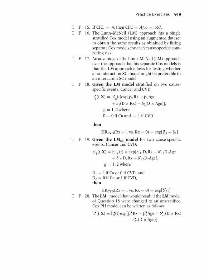
Practice Exercises 449
T F 15. If CICc = .4, then CPC = .4/.6 = .667.T F 16. The Lunn–McNeil (LM) approach fits a single
stratified Cox model using an augmented datasetto obtain the same results as obtained by fittingseparate Cox models for each cause-specific com-peting risk.
T F 17. An advantage of the Lunn–McNeil (LM) approachover the approach that fits separate Cox models isthat the LM approach allows for testing whethera no-interaction SC model might be preferable toan interaction SC model.
T F 18. Given the LM model stratified on two cause-specific events, Cancer and CVD:
h∗g(t,X) = h∗
0g(t)exp[β1Rx + β2Age
+ δ1(D × Rx) + δ2(D × Age)],g = 1, 2 whereD = 0 if Ca and = 1 if CVD
then
HRCVD(Rx = 1 vs. Rx = 0) = exp[β1 + δ1]
T F 19. Given the LMalt model for two cause-specificevents, Cancer and CVD:
h′g(t,X) = h′
0g (t) × exp[δ′11D1Rx + δ′
12D1Age+ δ′
21D2Rx + δ′22D2Age],
g = 1, 2 where
D1 = 1 if Ca or 0 if CVD, andD2 = 0 if Ca or 1 if CVD,then
HRCVD(Rx = 1 vs. Rx = 0) = exp[δ′21]
T F 20. The LMU model that would result if the LM modelof Question 18 were changed to an unstratifiedCox PH model can be written as follows.
h•(t,X) = h•0(t) exp[β•
1Rx + β•2Age + δ•
21(D × Rx)+ δ•
22(D × Age)]
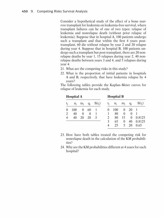
450 9. Competing Risks Survival Analysis
Consider a hypothetical study of the effect of a bone mar-row transplant for leukemia on leukemia-free survival, wheretransplant failures can be of one of two types: relapse ofleukemia and nonrelapse death (without prior relapse ofleukemia). Suppose that in hospital A, 100 patients undergosuch a transplant and that within the first 4 years post-transplant, 60 die without relapse by year 2 and 20 relapseduring year 4. Suppose that in hospital B, 100 patients un-dergo such a transplant but post-transplant, there are 20 non-relapse deaths by year 1, 15 relapses during year 2, 40 non-relapse deaths between years 3 and 4, and 5 relapses duringyear 4.21. What are the competing risks in this study?22. What is the proportion of initial patients in hospitals
A and B, respectively, that have leukemia relapse by 4years?
The following tables provide the Kaplan–Meier curves forrelapse of leukemia for each study.
Hospital A
tj nj mj qj S(tj)
0 100 0 60 12 40 0 0 14 40 20 20 .5
Hospital B
tj nj mj qj S(tj)
0 100 0 20 11 80 0 0 12 80 15 0 0.81253 65 0 40 0.81254 25 5 20 0.65
23. How have both tables treated the competing risk fornonrelapse death in the calculation of the KM probabili-ties?
24. Why are the KM probabilities different at 4 years for eachhospital?

Practice Exercises 451
25. Compute the CIC curves for each hospital using thefollowing tables.
Hospital A
tj nj mj hca(tj) S(tj−1) ˆIca(tj) CIC(tj)
0 100 0 02 40 0 0 1 0 04 40 20
Hospital B
tj nj mj hca(tj) S(tj−1) ˆIca(tj) CIC(tj)
0 100 0 01 80 0 0 1 0 02 80 153 65 04 25 5
26. Why are the CIC probabilities the same at 4 years?Consider a hypothetical study to assess the effect of a newhospital infection control strategy for patients who undergoheart transplant surgery in a given hospital. The exposurevariable of interest is a binary variable Group (G): G = 0 forthose patients receiving heart transplants from 1992 through1995 when the previous hospital control strategy was used;G = 1 for those patients receiving heart transplants from1996 through 1999 when the new hospital infection controlstrategy was adopted. The primary event of interest is gettinga hospital infection after surgery. A competing risk is deathduring recovery from surgery without getting a hospital infec-tion. Control variables being considered are tissue mismatchscore (TMS) at transplant and AGE at transplant. The out-come variable of interest is time (DAYS after surgery) until apatient developed a hospital infection.27. State a cause-specific no-interaction Cox PH model for
assessing the effect of group status (G) on time until ahospital infection event.
28. When fitting the model given in Question 27, which pa-tients should be considered censored?
29. Describe or provide a table that would show how the dataon the ith patient should be augmented for input into aLunn–McNeil (LM) model for this analysis.
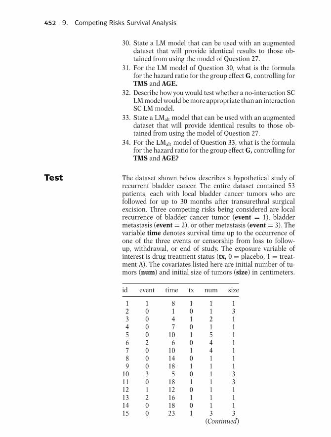
452 9. Competing Risks Survival Analysis
30. State a LM model that can be used with an augmenteddataset that will provide identical results to those ob-tained from using the model of Question 27.
31. For the LM model of Question 30, what is the formulafor the hazard ratio for the group effect G, controlling forTMS and AGE.
32. Describe how you would test whether a no-interaction SCLM model would be more appropriate than an interactionSC LM model.
33. State a LMalt model that can be used with an augmenteddataset that will provide identical results to those ob-tained from using the model of Question 27.
34. For the LMalt model of Question 33, what is the formulafor the hazard ratio for the group effect G, controlling forTMS and AGE?
Test The dataset shown below describes a hypothetical study ofrecurrent bladder cancer. The entire dataset contained 53patients, each with local bladder cancer tumors who arefollowed for up to 30 months after transurethral surgicalexcision. Three competing risks being considered are localrecurrence of bladder cancer tumor (event = 1), bladdermetastasis (event = 2), or other metastasis (event = 3). Thevariable time denotes survival time up to the occurrence ofone of the three events or censorship from loss to follow-up, withdrawal, or end of study. The exposure variable ofinterest is drug treatment status (tx, 0 = placebo, 1 = treat-ment A), The covariates listed here are initial number of tu-mors (num) and initial size of tumors (size) in centimeters.
id event time tx num size
1 1 8 1 1 12 0 1 0 1 33 0 4 1 2 14 0 7 0 1 15 0 10 1 5 16 2 6 0 4 17 0 10 1 4 18 0 14 0 1 19 0 18 1 1 1
10 3 5 0 1 311 0 18 1 1 312 1 12 0 1 113 2 16 1 1 114 0 18 0 1 115 0 23 1 3 3
(Continued)

Test 453
(Continued)
id event time tx num size
16 3 10 0 1 317 1 15 1 1 318 0 23 0 1 319 2 3 1 1 120 3 16 0 1 121 1 23 1 1 122 1 3 0 3 123 2 9 1 3 124 2 21 0 3 125 0 23 1 3 126 3 7 0 2 327 3 10 1 2 328 1 16 0 2 329 1 24 1 2 330 1 3 0 1 131 2 15 1 1 132 2 25 0 1 133 0 26 1 1 234 1 1 0 8 135 0 26 1 8 136 1 2 0 1 437 1 26 1 1 438 1 25 0 1 239 0 28 1 1 240 0 29 0 1 441 0 29 1 1 242 0 29 0 4 143 3 28 1 1 644 1 30 0 1 645 2 2 1 1 546 1 17 0 1 547 1 22 1 1 548 0 30 0 1 549 3 3 1 2 150 2 6 0 2 151 3 8 1 2 152 3 12 0 2 153 0 30 1 2 1
1. Suppose you wish to use these data to determine the ef-fect of tx on survival time for the cause-specific event of alocal recurrence of bladder cancer. State a no-interactionCox PH model for assessing this relationship that adjustsfor the covariates num and size.

454 9. Competing Risks Survival Analysis
2. When fitting the model given in Question 1, which sub-jects are considered censored?
3. How would you modify your answers to Questions 1 and2 if you were interested in the effect of tx on survival timefor the cause-specific event of finding metastatic bladdercancer?
4. For the model considered in Question 1, briefly describehow to carry out a sensitivity analysis to determine howbadly the results from fitting this model might be biasedif the assumption of independent competing risks is vi-olated.
5. The following two tables provide information necessaryfor calculating CIC curves for local recurrence of bladdercancer (event = 1) separately for each treatment group.The CIC formula used for both tables is given by theexpression
CIC1(tj) =j∑
j′=1
I1(t′j) =j∑
j′=1
S(tj′−1)h1(tj′)
where h1(tj) = m1j/nj, m1j is the number of local recur-rent failures at time tj, and S(tj−1) is the overall (event-free) survival probability for failure from either of thetwo competing risks at time tj−1.
tx = 1 (Treatment A)
tj nj d1j h1(tj) S(tj−1) I1(tj) CIC1(tj)
0 27 0 0 — — —2 27 0 0 1 0 03 26 0 0 .9630 0 04 24 0 0 .8889 0 08 23 1 .0435 .8889 .0387 .03879 21 0 0 .8116 0 .0387
10 20 0 0 .7729 0 .038715 17 1 .0588 .7343 .0432 .081916 15 0 0 .6479 0 .081918 14 0 0 .6047 0 .081922 12 1 .0833 .6047 .0504 .132323 11 1 .0910 .5543 .0504 .182724 8 1 .1250 .5039 .0630 .245726 7 1 .1429 .4409 .0630 .308728 4 0 0 .3779 0 .308729 2 0 0 .2835 0 .308730 1 0 0 .2835 0 .3087

Test 455
tx = 1 (Placebo)
tj nj d1j h1(tj) S(tj−1) I1(tj) CIC1(tj)
0 26 0 0 — — —1 26 1 .0400 1 .0400 .04002 24 1 .0417 .9615 .0400 .08003 23 2 .0870 .9215 .0801 .16015 21 0 0 .8413 0 .16016 20 0 0 .8013 0 .16017 18 0 0 .7212 0 .1601
10 16 0 0 .6811 0 .160112 15 1 .0667 .6385 .0426 .202714 13 0 0 .6835 0 .202716 12 1 .0833 .5534 .0461 .248817 10 1 .1000 .4612 .0461 .294918 9 0 0 .4150 0 .294921 8 0 0 .4150 0 .294923 7 0 0 .3632 0 .294925 6 1 .1667 .3632 .0605 .355429 4 0 0 .2421 0 .355430 2 1 0 .2421 0 .3554
a. Verify the CIC1 calculation provided at failure timetj = 8 for persons in the treatment group (tx = 1); thatis, use the original data to compute h1(tj), S(tj−1),I1(tj), and CIC1(tj), assuming that the calculationsmade up to this failure time are correct.
b. Verify the CIC1 calculation provided at failure timetj = 25 for persons in the placebo group (tx = 0).
c. Interpret the CIC1 values obtained for both the treat-ment and placebo groups at tj = 30.
d. How can you calculate the CPC1 values for both treat-ment and placebo groups at tj = 30?

456 9. Competing Risks Survival Analysis
6. The following output was obtained using separatemodels for each of the 3 event-types.
Event = 1
Var DF Coef Std.Err. p > |z| Haz.ratio
tx 1 −0.6258 0.5445 0.2504 0.535num 1 0.0243 0.1900 0.8983 1.025size 1 0.0184 0.1668 0.9120 1.125
Event = 2
Var DF Coef Std.Err. p > |z| Haz.ratio
tx 1 −0.0127 0.6761 0.9851 0.987num 1 −0.1095 0.2281 0.6312 0.896size 1 −0.6475 0.3898 0.0966 0.523
Event = 3
Var DF Coef Std.Err. p > |z| Haz.ratio
tx 1 −0.3796 0.6770 0.5750 0.684num 1 −0.1052 0.3135 0.7372 0.900size 1 −0.0238 0.2177 0.9128 0.976
a. What is the effect of treatment on survival from hav-ing a local recurrence of bladder cancer, and is itsignificant?
b. What is the effect of treatment on survival from de-veloping metastatic bladder cancer, and is it signifi-cant?
c. What is the effect of treatment on survival from othermetastatic cancer, and is it significant?
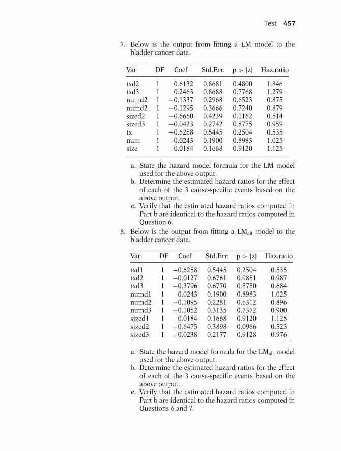
Test 457
7. Below is the output from fitting a LM model to thebladder cancer data.
Var DF Coef Std.Err. p > |z| Haz.ratio
txd2 1 0.6132 0.8681 0.4800 1.846txd3 1 0.2463 0.8688 0.7768 1.279numd2 1 −0.1337 0.2968 0.6523 0.875numd2 1 −0.1295 0.3666 0.7240 0.879sized2 1 −0.6660 0.4239 0.1162 0.514sized3 1 −0.0423 0.2742 0.8775 0.959tx 1 −0.6258 0.5445 0.2504 0.535num 1 0.0243 0.1900 0.8983 1.025size 1 0.0184 0.1668 0.9120 1.125
a. State the hazard model formula for the LM modelused for the above output.
b. Determine the estimated hazard ratios for the effectof each of the 3 cause-specific events based on theabove output.
c. Verify that the estimated hazard ratios computed inPart b are identical to the hazard ratios computed inQuestion 6.
8. Below is the output from fitting a LMalt model to thebladder cancer data.
Var DF Coef Std.Err. p > |z| Haz.ratio
txd1 1 −0.6258 0.5445 0.2504 0.535txd2 1 −0.0127 0.6761 0.9851 0.987txd3 1 −0.3796 0.6770 0.5750 0.684numd1 1 0.0243 0.1900 0.8983 1.025numd2 1 −0.1095 0.2281 0.6312 0.896numd3 1 −0.1052 0.3135 0.7372 0.900sized1 1 0.0184 0.1668 0.9120 1.125sized2 1 −0.6475 0.3898 0.0966 0.523sized3 1 −0.0238 0.2177 0.9128 0.976
a. State the hazard model formula for the LMalt modelused for the above output.
b. Determine the estimated hazard ratios for the effectof each of the 3 cause-specific events based on theabove output.
c. Verify that the estimated hazard ratios computed inPart b are identical to the hazard ratios computed inQuestions 6 and 7.
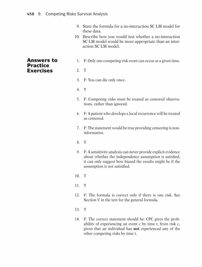
458 9. Competing Risks Survival Analysis
9. State the formula for a no-interaction SC LM model forthese data.
10. Describe how you would test whether a no-interactionSC LM model would be more appropriate than an inter-action SC LM model.
Answers toPracticeExercises
1. F: Only one competing risk event can occur at a given time.
2. T
3. F: You can die only once.
4. T
5. F: Competing risks must be treated as censored observa-tions, rather than ignored.
6. F: A patient who develops a local recurrence will be treatedas censored.
7. F: The statement would be true providing censoring is non-informative.
8. T
9. F: A sensitivity analysis can never provide explicit evidenceabout whether the independence assumption is satisfied;it can only suggest how biased the results might be if theassumption is not satisified.
10. T
11. T
12. F: The formula is correct only if there is one risk. SeeSection V in the text for the general formula.
13. T
14. F: The correct statement should be: CPC gives the prob-ability of experiencing an event c by time t, from risk c,given that an individual has not experienced any of theother competing risks by time t.

Answers to Practice Exercises 459
15. F: the correct formula for CPC is: CPCc = CICc/(1 − CICc′ )where CICc = .4 and CICc′ = CIC from risks other than c,where the latter is not necessarily equal to .4.
16. T
17. T
18. T
19. T.
20. F: The correct LMU model ish•(t,X) = h•
0(t) exp[γ1D + β•1Rx + β•
2Age + δ•21(D × Rx)
+ δ•22(D × Age)]
21. The competing risks are (1) relapse of leukemia and (2)nonrelapse death.
22. 20/100 = 0.2.
23. Both tables have treated the competing risks as if they werecensored observations.
24. The KM probabilities are different for the two hospitalsbecause the competing risks contribute a different patternof censorship in the two hospitals.
25. The CIC curves for each hospital are calculated as follows.
Hospital A
tj nj mj hca(tj) S(tj−1) Ica(tj) CIC(tj)
0 100 0 0 — — —2 40 0 0 1 0 04 40 20 0.5 0.4 0.20 0.20
Hospital B
tj nj mj hca(tj) S(tj−1) Ica(tj) CIC(tj)
0 100 0 0 — — —1 80 0 0 1 0 02 80 15 0.1875 0.8 0.15 0.153 65 0 0 0.65 0 0.154 25 5 0.20 0.25 0.05 0.20
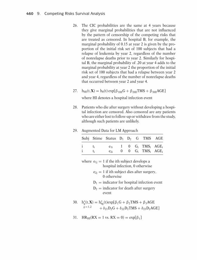
460 9. Competing Risks Survival Analysis
26. The CIC probabilities are the same at 4 years becausethey give marginal probabilities that are not influencedby the pattern of censorship of the competing risks thatare treated as censored. In hospital B, for example, themarginal probability of 0.15 at year 2 is given by the pro-portion of the initial risk set of 100 subjects that had arelapse of leukemia by year 2, regardless of the numberof nonrelapse deaths prior to year 2. Similarly for hospi-tal B, the marginal probability of .20 at year 4 adds to themarginal probability at year 2 the proportion of the initialrisk set of 100 subjects that had a relapse between year 2and year 4, regardless of the number of nonrelapse deathsthat occurred between year 2 and year 4.
27. hHI(t,X) = h0(t) exp[β1HIG + β2HITMS + β3HIAGE]
where HI denotes a hospital infection event
28. Patients who die after surgery without developing a hospi-tal infection are censored. Also censored are any patientswho are either lost to follow-up or withdraw from the study,although such patients are unlikely.
29. Augmented Data for LM Approach
Subj Stime Status D1 D2 G TMS AGE
i ti e1i 1 0 Gi TMSi AGEi
i ti e2i 0 0 Gi TMSi AGEi
where e1j = 1 if the ith subject develops ahospital infection, 0 otherwise
e2j = 1 if ith subject dies after surgery,0 otherwise
D1 = indicator for hospital infection event
D2 = indicator for death after surgeryevent
30. h∗g(t,X)g = 1,2
= h∗0g(t)exp[β1G + β2TMS + β3AGE
+ δ21D2G + δ22D2TMS + δ23D2AGE]
31. HRHI(RX = 1 vs. RX = 0) = exp[β1]

Answers to Practice Exercises 461
32. Carry out a likelihood ratio test to compare the followingtwo models. Full (SC Interaction LM) model:h∗
g(t,X)g = 1,2
= h∗0g(t)exp[β1G + β2TMS + β3AGE
+ δ21D2G + δ22D2TMS + δ23D2AGE]
Reduced (no-interaction SC LM) model:h∗
g(t,X)g = 1,2
= h∗0g(t)exp[β1G + β2TMS + β3AGE]
LR test statistic= −2 ln LR − (−2 ln LF) is distributed χ23
under H0: no-interaction model
33. h′g(t,X)g = 1,2
= h′0g(t)exp[β′
1D1G + β′2D1TMS + β′
3D1AGE
+ δ′21D2G + δ′
22D2TMS + δ′23D2AGE]
34. HRHI(RX = 1 vs. RX = 0) = exp[β′1]

ComputerAppendix:SurvivalAnalysison theComputerIn this appendix, we provide examples of computer programsfor carrying out the survival analyses described in this text.This appendix does not give an exhaustive survey of all com-puter packages currently available, but rather is intended todescribe the similarities and differences among three of themost widely used packages. The software packages that wedescribe are Stata (version 7.0), SAS (version 8.2), and SPSS(version 11.5). A complete description of these packages is be-yond the scope of this appendix. Readers are referred to thebuilt-in Help functions for each program for further informa-tion.
463

464 Computer Appendix: Survival Analysis on the Computer
Datasets
Most of the computer syntax and output presented in this ap-pendix are obtained from running step-by-step survival anal-yses on the “addicts” dataset. The other dataset that is utilizedin this appendix is the “bladder cancer” dataset for analysesof recurrent events. The addicts and bladder cancer data aredescribed below and can be downloaded from our Web siteat http://www.sph.emory.edu/∼dkleinb/surv2.htm. On thisWeb site we also provide many of the other datasets that havebeen used in the examples and exercises throughout this text.The data on our Web site are provided in several forms: (1) asStata datasets (with a .dta extension), (2) as SAS version 8.2datasets (with a .sas7bdat extension), (3) as SPSS datasets(with a .sav extension), and (4) as text datasets (with a .datextension).
Addicts Dataset (addicts.dat)
In a 1991 Australian study by Caplehorn et al., two methadonetreatment clinics for heroin addicts were compared to assesspatient time remaining under methadone treatment. A pa-tient’s survival time was determined as the time, in days, untilthe person dropped out of the clinic or was censored. The twoclinics differed according to their live-in policies for patients.The variables are defined as follows.
ID—Patient ID.SURVT—The time (in days) until the patient dropped out of the
clinic or was censored.STATUS—Indicates whether the patient dropped out of the clinic
(coded 1) or was censored (coded 0).CLINIC—Indicates which methadone treatment clinic the pa-
tient attended (coded 1 or 2).PRISON—Indicates whether the patient had a prison record
(coded 1) or not (coded 0).DOSE—A continuous variable for the patient’s maximum
methadone dose (mg/day).
Bladder Cancer Dataset (bladder.dat)
The bladder cancer dataset contains recurrent event outcomeinformation for 86 cancer patients followed for the recurrenceof bladder cancer tumor after transurethral surgical excision(Byar and Green, 1980). The exposure of interest is the effectof the drug treatment of thiotepa. Control variables are theinitial number and initial size of tumors. The data layout issuitable for a counting processes approach. The variables aredefined as follows.

Stata Computer Appendix: Survival Analysis on the Computer 465
ID—Patient ID (may have multiple observations for the samesubject).
EVENT—Indicates whether the patient had a tumor (coded 1) ornot (coded 0).
INTERVAL—A counting number representing the order of thetime interval for a given subject (coded 1 for the subject’s firsttime interval, 2 for a subject’s second time interval, etc.).
START—The starting time (in months) for each interval.STOP—The time of event (in months) or censorship for each
interval.TX—Treatment status (coded 1 for treatment with thiotepa and
0 for the placebo).NUM—The initial number of tumor(s).SIZE—The initial size (in centimeters) of the tumor.
Software
What follows is a detailed explanation of the code and outputnecessary to perform the type of survival analyses described inthis text. The rest of this appendix is divided into three broadsections, one for each of the following software packages,
A. Stata,B. SAS, andC. SPSS.
Each of these sections is self-contained, allowing the readerto focus on the particular statistical package of his or herinterest.
A. StataAnalyses using Stata are obtained by typing the appropriatestatistical commands in the Stata Command window or in theStata Do-file Editor window. The key commands used to per-form the survival analyses are listed below. These commandsare case sensitive and lowercase letters should be used.
stset—Declares data in memory to be survival data. Used todefine the “time-to-event” variable, the “status” variable, andother relevant survival variables. Other Stata commands be-ginning with st utilize these defined variables.
sts list—Produces Kaplan–Meier (KM) or Cox adjusted survivalestimates in the output window. The default is KM survivalestimates.
sts graph—Produces plots of Kaplan–Meier (KM) survival es-timates. This command can also be used to produce Cox ad-justed survival plots.
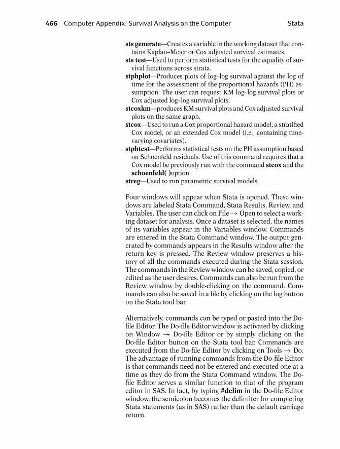
466 Computer Appendix: Survival Analysis on the Computer Stata
sts generate—Creates a variable in the working dataset that con-tains Kaplan–Meier or Cox adjusted survival estimates.
sts test—Used to perform statistical tests for the equality of sur-vival functions across strata.
stphplot—Produces plots of log–log survival against the log oftime for the assessment of the proportional hazards (PH) as-sumption. The user can request KM log–log survival plots orCox adjusted log–log survival plots.
stcoxkm—produces KM survival plots and Cox adjusted survivalplots on the same graph.
stcox—Used to run a Cox proportional hazard model, a stratifiedCox model, or an extended Cox model (i.e., containing time-varying covariates).
stphtest—Performs statistical tests on the PH assumption basedon Schoenfeld residuals. Use of this command requires that aCox model be previously run with the command stcox and theschoenfeld( )option.
streg—Used to run parametric survival models.
Four windows will appear when Stata is opened. These win-dows are labeled Stata Command, Stata Results, Review, andVariables. The user can click on File → Open to select a work-ing dataset for analysis. Once a dataset is selected, the namesof its variables appear in the Variables window. Commandsare entered in the Stata Command window. The output gen-erated by commands appears in the Results window after thereturn key is pressed. The Review window preserves a his-tory of all the commands executed during the Stata session.The commands in the Review window can be saved, copied, oredited as the user desires. Commands can also be run from theReview window by double-clicking on the command. Com-mands can also be saved in a file by clicking on the log buttonon the Stata tool bar.
Alternatively, commands can be typed or pasted into the Do-file Editor. The Do-file Editor window is activated by clickingon Window → Do-file Editor or by simply clicking on theDo-file Editor button on the Stata tool bar. Commands areexecuted from the Do-file Editor by clicking on Tools → Do.The advantage of running commands from the Do-file Editoris that commands need not be entered and executed one at atime as they do from the Stata Command window. The Do-file Editor serves a similar function to that of the programeditor in SAS. In fact, by typing #delim in the Do-file Editorwindow, the semicolon becomes the delimiter for completingStata statements (as in SAS) rather than the default carriagereturn.
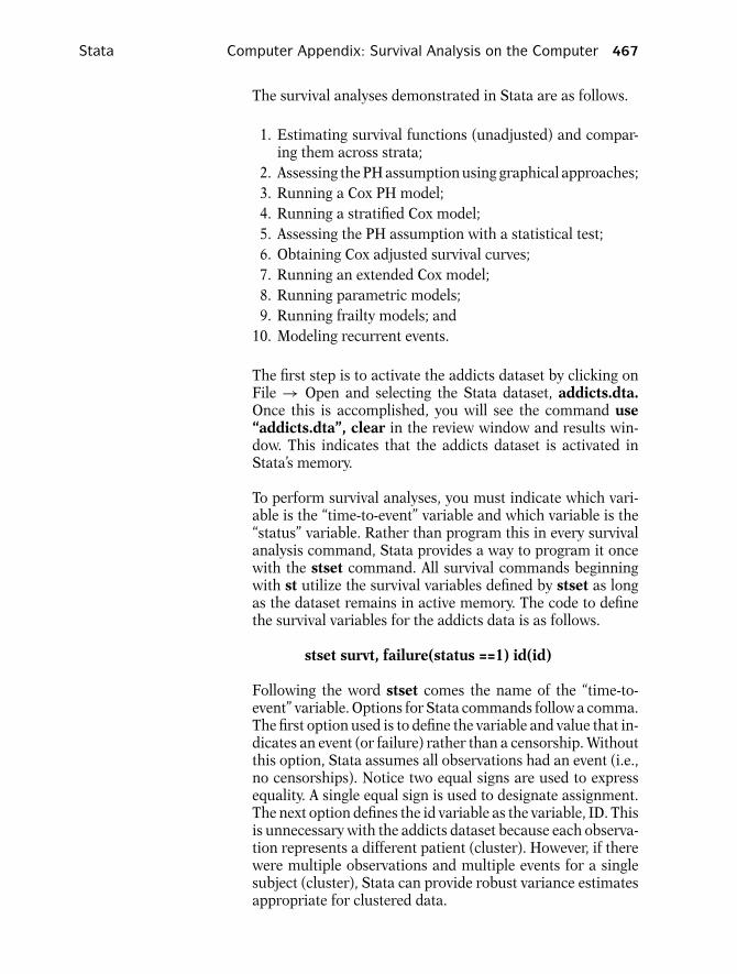
Stata Computer Appendix: Survival Analysis on the Computer 467
The survival analyses demonstrated in Stata are as follows.
1. Estimating survival functions (unadjusted) and compar-ing them across strata;
2. Assessing the PH assumption using graphical approaches;3. Running a Cox PH model;4. Running a stratified Cox model;5. Assessing the PH assumption with a statistical test;6. Obtaining Cox adjusted survival curves;7. Running an extended Cox model;8. Running parametric models;9. Running frailty models; and
10. Modeling recurrent events.
The first step is to activate the addicts dataset by clicking onFile → Open and selecting the Stata dataset, addicts.dta.Once this is accomplished, you will see the command use“addicts.dta”, clear in the review window and results win-dow. This indicates that the addicts dataset is activated inStata’s memory.
To perform survival analyses, you must indicate which vari-able is the “time-to-event” variable and which variable is the“status” variable. Rather than program this in every survivalanalysis command, Stata provides a way to program it oncewith the stset command. All survival commands beginningwith st utilize the survival variables defined by stset as longas the dataset remains in active memory. The code to definethe survival variables for the addicts data is as follows.
stset survt, failure(status ==1) id(id)
Following the word stset comes the name of the “time-to-event” variable. Options for Stata commands follow a comma.The first option used is to define the variable and value that in-dicates an event (or failure) rather than a censorship. Withoutthis option, Stata assumes all observations had an event (i.e.,no censorships). Notice two equal signs are used to expressequality. A single equal sign is used to designate assignment.The next option defines the id variable as the variable, ID. Thisis unnecessary with the addicts dataset because each observa-tion represents a different patient (cluster). However, if therewere multiple observations and multiple events for a singlesubject (cluster), Stata can provide robust variance estimatesappropriate for clustered data.
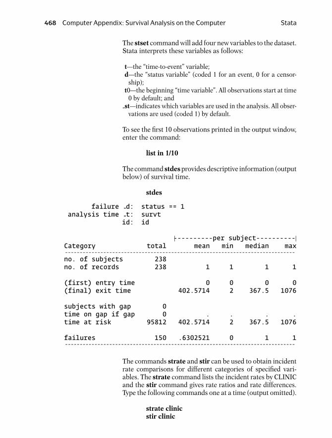
468 Computer Appendix: Survival Analysis on the Computer Stata
The stset command will add four new variables to the dataset.Stata interprets these variables as follows:
t—the “time-to-event” variable;d—the “status variable” (coded 1 for an event, 0 for a censor-
ship);t0—the beginning “time variable”. All observations start at time
0 by default; andst—indicates which variables are used in the analysis. All obser-
vations are used (coded 1) by default.
To see the first 10 observations printed in the output window,enter the command:
list in 1/10
The command stdes provides descriptive information (outputbelow) of survival time.
stdes
failure -d: status == 1analysis time -t: survt
id: id
----------per subject----------| |Category total mean min median max- - - - - - - - - - - - - - - - - - - - - - - - - - - - - - - - - - - - - - - - - - - - - - - - - - - - - - - - - - - - - - - - - - - - - - - - - - - - - -no. of subjects 238no. of records 238 1 1 1 1
(first) entry time 0 0 0 0(final) exit time 402.5714 2 367.5 1076
subjects with gap 0time on gap if gap 0 . . . .time at risk 95812 402.5714 2 367.5 1076
failures 150 .6302521 0 1 1- - - - - - - - - - - - - - - - - - - - - - - - - - - - - - - - - - - - - - - - - - - - - - - - - - - - - - - - - - - - - - - - - - - - - - - - - - - - - -
The commands strate and stir can be used to obtain incidentrate comparisons for different categories of specified vari-ables. The strate command lists the incident rates by CLINICand the stir command gives rate ratios and rate differences.Type the following commands one at a time (output omitted).
strate clinicstir clinic
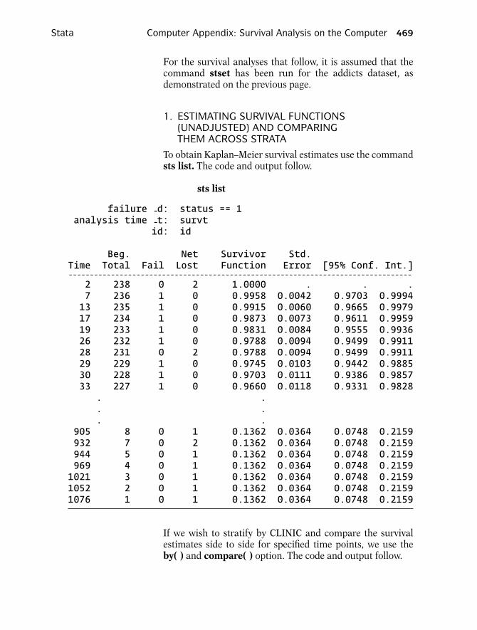
Stata Computer Appendix: Survival Analysis on the Computer 469
For the survival analyses that follow, it is assumed that thecommand stset has been run for the addicts dataset, asdemonstrated on the previous page.
1. ESTIMATING SURVIVAL FUNCTIONS(UNADJUSTED) AND COMPARINGTHEM ACROSS STRATA
To obtain Kaplan–Meier survival estimates use the commandsts list. The code and output follow.
sts list
failure -d: status == 1analysis time -t: survt
id: id
Beg. Net Survivor Std.Time Total Fail Lost Function Error [95% Conf. Int.]- - - - - - - - - - - - - - - - - - - - - - - - - - - - - - - - - - - - - - - - - - - - - - - - - - - - - - - - - - - - - - - - - - - - - - - - - - - - - - - - -2 238 0 2 1.0000 . . .7 236 1 0 0.9958 0.0042 0.9703 0.999413 235 1 0 0.9915 0.0060 0.9665 0.997917 234 1 0 0.9873 0.0073 0.9611 0.995919 233 1 0 0.9831 0.0084 0.9555 0.993626 232 1 0 0.9788 0.0094 0.9499 0.991128 231 0 2 0.9788 0.0094 0.9499 0.991129 229 1 0 0.9745 0.0103 0.9442 0.988530 228 1 0 0.9703 0.0111 0.9386 0.985733 227 1 0 0.9660 0.0118 0.9331 0.9828. .. .. .
905 8 0 1 0.1362 0.0364 0.0748 0.2159932 7 0 2 0.1362 0.0364 0.0748 0.2159944 5 0 1 0.1362 0.0364 0.0748 0.2159969 4 0 1 0.1362 0.0364 0.0748 0.21591021 3 0 1 0.1362 0.0364 0.0748 0.21591052 2 0 1 0.1362 0.0364 0.0748 0.21591076 1 0 1 0.1362 0.0364 0.0748 0.2159
If we wish to stratify by CLINIC and compare the survivalestimates side to side for specified time points, we use theby( ) and compare( ) option. The code and output follow.

470 Computer Appendix: Survival Analysis on the Computer Stata
sts list, by(clinic) compare at (0 20 to 1080)
failure -d: status == 1analysis time -t: survt
id: id
Survivor Functionclinic 1 2- - - - - - - - - - - - - - - - - - - - - - - - - - - - - - - - - - - - - - - - - - - - - -time 0 1.0000 1.0000
20 0.9815 0.986540 0.9502 0.959560 0.9189 0.945980 0.9000 0.9320100 0.8746 0.9320120 0.8681 0.9179140 0.8422 0.9038160 0.8093 0.8753180 0.7690 0.8466200 0.7420 0.8323220 0.6942 0.8179
.
.
.840 0.0725 0.5745860 0.0543 0.5745880 0.0543 0.5171900 0.0181 0.5171920 . 0.5171940 . 0.5171960 . 0.5171980 . 0.51711000 . 0.51711020 . 0.51711040 . 0.51711060 . 0.51711080 . .
Notice that the survival rate for CLINIC = 2 is higher thanCLINIC = 1. Other survival times could have been requestedusing the compare( ) option.
To graph the Kaplan–Meier survival function (against time),use the code
sts graph

Stata Computer Appendix: Survival Analysis on the Computer 471
The code and output that provide a graph of the Kaplan–Meiersurvival function stratified by CLINIC follow.
sts graph, by(clinic)
clinic 2
clinic 1
0
0.00
0.25
0.50
0.75
1.00
500 1000
Kaplan-Meier survival estimates, by clinic
analysis time
The failure option graphs the failure function (the cumulativerisk) rather than the survival (zero to one rather than one tozero). The code follows (output omitted).
sts graph, by(clinic) failure
The code to run the log rank test on the variable CLINIC (andoutput) follows.
sts test clinic
failure -d: status == 1analysis time -t: survt
id: id
Log-rank test for equality of survivor functions
Events Eventsclinic observed expected- - - - - - - - - - - - - - - - - - - - - - - - - - - - - - - - - - - -1 122 90.912 28 59.09- - - - - - - - - - - - - - - - - - - - - - - - - - - - - - - - - - - -Total 150 150.00
chi2(1) = 27.89Pr>chi2 = 0.0000
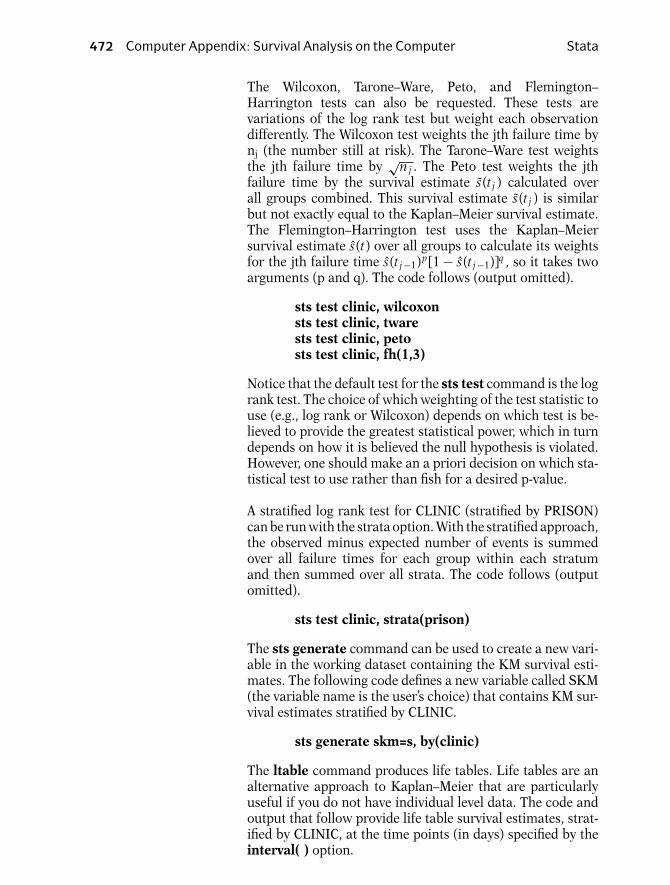
472 Computer Appendix: Survival Analysis on the Computer Stata
The Wilcoxon, Tarone–Ware, Peto, and Flemington–Harrington tests can also be requested. These tests arevariations of the log rank test but weight each observationdifferently. The Wilcoxon test weights the jth failure time bynj (the number still at risk). The Tarone–Ware test weightsthe jth failure time by
√n j . The Peto test weights the jth
failure time by the survival estimate s(t j ) calculated overall groups combined. This survival estimate s(t j ) is similarbut not exactly equal to the Kaplan–Meier survival estimate.The Flemington–Harrington test uses the Kaplan–Meiersurvival estimate s(t) over all groups to calculate its weightsfor the jth failure time s(t j−1)p[1 − s(t j−1)]q , so it takes twoarguments (p and q). The code follows (output omitted).
sts test clinic, wilcoxonsts test clinic, twarests test clinic, petosts test clinic, fh(1,3)
Notice that the default test for the sts test command is the logrank test. The choice of which weighting of the test statistic touse (e.g., log rank or Wilcoxon) depends on which test is be-lieved to provide the greatest statistical power, which in turndepends on how it is believed the null hypothesis is violated.However, one should make an a priori decision on which sta-tistical test to use rather than fish for a desired p-value.
A stratified log rank test for CLINIC (stratified by PRISON)can be run with the strata option. With the stratified approach,the observed minus expected number of events is summedover all failure times for each group within each stratumand then summed over all strata. The code follows (outputomitted).
sts test clinic, strata(prison)
The sts generate command can be used to create a new vari-able in the working dataset containing the KM survival esti-mates. The following code defines a new variable called SKM(the variable name is the user’s choice) that contains KM sur-vival estimates stratified by CLINIC.
sts generate skm=s, by(clinic)
The ltable command produces life tables. Life tables are analternative approach to Kaplan–Meier that are particularlyuseful if you do not have individual level data. The code andoutput that follow provide life table survival estimates, strat-ified by CLINIC, at the time points (in days) specified by theinterval( ) option.
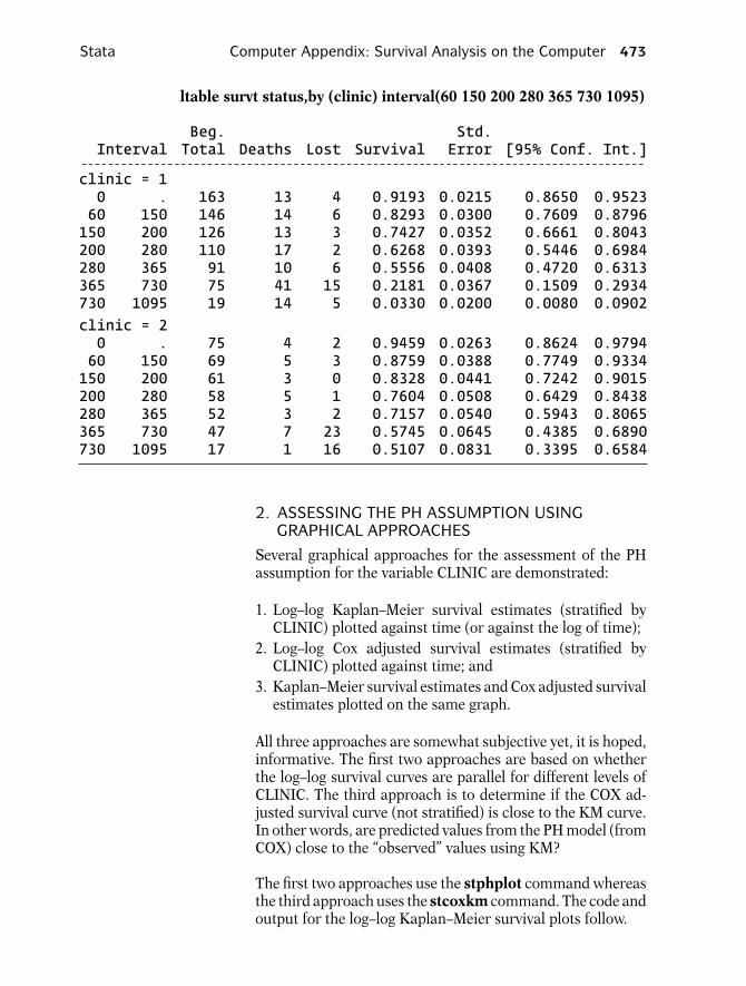
Stata Computer Appendix: Survival Analysis on the Computer 473
ltable survt status,by (clinic) interval(60 150 200 280 365 730 1095)
Beg. Std.Interval Total Deaths Lost Survival Error [95% Conf. Int.]
- - - - - - - - - - - - - - - - - - - - - - - - - - - - - - - - - - - - - - - - - - - - - - - - - - - - - - - - - - - - - - - - - - - - - - - - - - - - - - - - - - - - -clinic = 10 . 163 13 4 0.9193 0.0215 0.8650 0.952360 150 146 14 6 0.8293 0.0300 0.7609 0.8796150 200 126 13 3 0.7427 0.0352 0.6661 0.8043200 280 110 17 2 0.6268 0.0393 0.5446 0.6984280 365 91 10 6 0.5556 0.0408 0.4720 0.6313365 730 75 41 15 0.2181 0.0367 0.1509 0.2934730 1095 19 14 5 0.0330 0.0200 0.0080 0.0902clinic = 20 . 75 4 2 0.9459 0.0263 0.8624 0.979460 150 69 5 3 0.8759 0.0388 0.7749 0.9334150 200 61 3 0 0.8328 0.0441 0.7242 0.9015200 280 58 5 1 0.7604 0.0508 0.6429 0.8438280 365 52 3 2 0.7157 0.0540 0.5943 0.8065365 730 47 7 23 0.5745 0.0645 0.4385 0.6890730 1095 17 1 16 0.5107 0.0831 0.3395 0.6584
2. ASSESSING THE PH ASSUMPTION USINGGRAPHICAL APPROACHES
Several graphical approaches for the assessment of the PHassumption for the variable CLINIC are demonstrated:
1. Log–log Kaplan–Meier survival estimates (stratified byCLINIC) plotted against time (or against the log of time);
2. Log–log Cox adjusted survival estimates (stratified byCLINIC) plotted against time; and
3. Kaplan–Meier survival estimates and Cox adjusted survivalestimates plotted on the same graph.
All three approaches are somewhat subjective yet, it is hoped,informative. The first two approaches are based on whetherthe log–log survival curves are parallel for different levels ofCLINIC. The third approach is to determine if the COX ad-justed survival curve (not stratified) is close to the KM curve.In other words, are predicted values from the PH model (fromCOX) close to the “observed” values using KM?
The first two approaches use the stphplot command whereasthe third approach uses the stcoxkm command. The code andoutput for the log–log Kaplan–Meier survival plots follow.
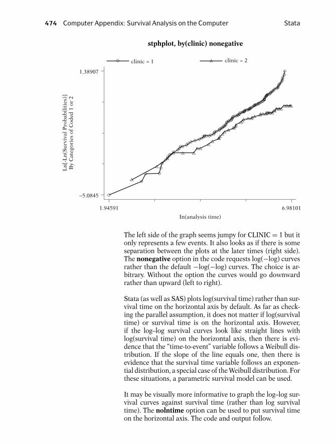
474 Computer Appendix: Survival Analysis on the Computer Stata
stphplot, by(clinic) nonegative
−5.0845
1.38907
1.94591 6.98101
In(analysis time)
Ln
[-L
n(S
urv
ival
Pro
bab
ilit
ies)
]B
y C
ateg
orie
s of
Cod
ed 1
or
2
clinic = 1 clinic = 2
The left side of the graph seems jumpy for CLINIC = 1 but itonly represents a few events. It also looks as if there is someseparation between the plots at the later times (right side).The nonegative option in the code requests log(−log) curvesrather than the default −log(−log) curves. The choice is ar-bitrary. Without the option the curves would go downwardrather than upward (left to right).
Stata (as well as SAS) plots log(survival time) rather than sur-vival time on the horizontal axis by default. As far as check-ing the parallel assumption, it does not matter if log(survivaltime) or survival time is on the horizontal axis. However,if the log–log survival curves look like straight lines withlog(survival time) on the horizontal axis, then there is evi-dence that the “time-to-event” variable follows a Weibull dis-tribution. If the slope of the line equals one, then there isevidence that the survival time variable follows an exponen-tial distribution, a special case of the Weibull distribution. Forthese situations, a parametric survival model can be used.
It may be visually more informative to graph the log–log sur-vival curves against survival time (rather than log survivaltime). The nolntime option can be used to put survival timeon the horizontal axis. The code and output follow.

Stata Computer Appendix: Survival Analysis on the Computer 475
stphplot, by(clinic) nonegative nolntime
clinic = 1 clinic = 21.38907
−5.0845
7 1076
Ln
[-L
n(S
urv
ival
Pro
bab
ilit
ies)
]B
y C
ateg
orie
s of
Cod
ed 1
or
2
analysis time
The graph suggests that the curves begin to diverge over time.
The stphplot command can also be used to obtain log–logCox adjusted survival estimates. The code follows.
stphplot, strata(clinic) adjust(prison dose) nonegative nolntime
The log–log curves are adjusted for PRISON and DOSE usinga stratified COX model on the variable CLINIC. The meanvalues of PRISON and DOSE are used for the adjustment.The output follows.
clinic = 1 clinic = 21.65856
−5.23278
7 1076
Ln
[-L
n(S
urv
ival
Pro
bab
ilit
ies)
]
By
Cat
egor
ies
of C
oded
1 o
r 2
analysis time
The Cox adjusted curves look very similar to the KM curves.
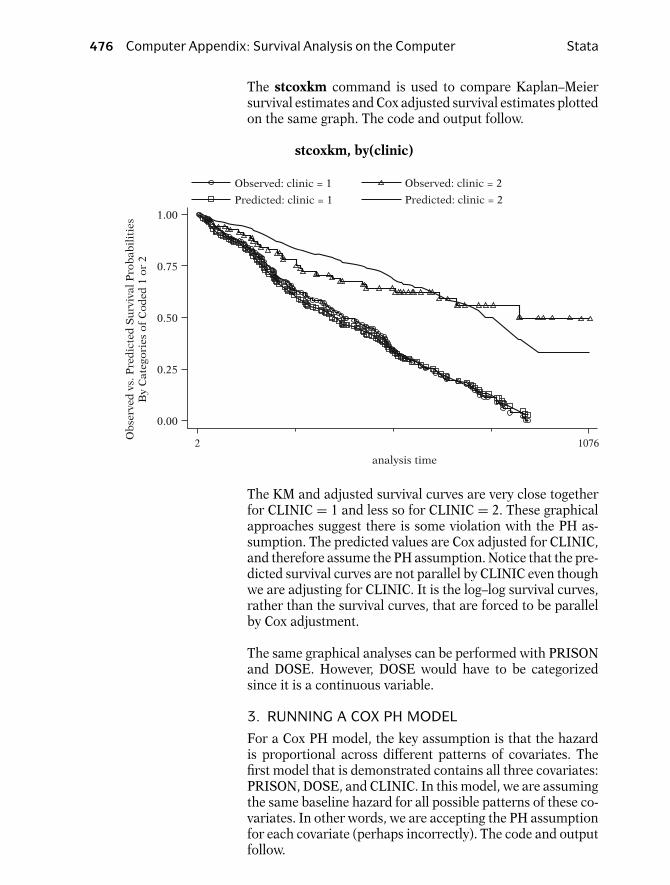
476 Computer Appendix: Survival Analysis on the Computer Stata
The stcoxkm command is used to compare Kaplan–Meiersurvival estimates and Cox adjusted survival estimates plottedon the same graph. The code and output follow.
stcoxkm, by(clinic)
Observed: clinic = 1
Predicted: clinic = 1
Observed: clinic = 2
Predicted: clinic = 2
0.00
0.25
0.50
0.75
1.00
2 1076Ob
serv
ed v
s. P
red
icte
d S
urv
ival
Pro
bab
ilit
ies
By
Cat
egor
ies
of C
oded
1 o
r 2
analysis time
The KM and adjusted survival curves are very close togetherfor CLINIC = 1 and less so for CLINIC = 2. These graphicalapproaches suggest there is some violation with the PH as-sumption. The predicted values are Cox adjusted for CLINIC,and therefore assume the PH assumption. Notice that the pre-dicted survival curves are not parallel by CLINIC even thoughwe are adjusting for CLINIC. It is the log–log survival curves,rather than the survival curves, that are forced to be parallelby Cox adjustment.
The same graphical analyses can be performed with PRISONand DOSE. However, DOSE would have to be categorizedsince it is a continuous variable.
3. RUNNING A COX PH MODEL
For a Cox PH model, the key assumption is that the hazardis proportional across different patterns of covariates. Thefirst model that is demonstrated contains all three covariates:PRISON, DOSE, and CLINIC. In this model, we are assumingthe same baseline hazard for all possible patterns of these co-variates. In other words, we are accepting the PH assumptionfor each covariate (perhaps incorrectly). The code and outputfollow.

Stata Computer Appendix: Survival Analysis on the Computer 477
stcox prison clinic dose, nohr
failure -d: status == 1analysis time -t: survt
id: id
Iteration 0: log likelihood = -705.6619Iteration 1: log likelihood = -674.54907Iteration 2: log likelihood = -673.407Iteration 3: log likelihood = -673.40242Iteration 4: log likelihood = -673.40242Refining estimates:Iteration 0: log likelihood = -673.40242
Cox regression -- Breslow method for ties
No. of subjects = 238 Number of obs = 238No. of failures = 150Time at risk = 95812
LR chi2(3) = 64.52Log likelihood = -673.40242 Prob > chi2 = 0.0000
- - - - - - - - - - - - - - - - - - - - - - - - - - - - - - - - - - - - - - - - - - - - - - - - - - - - - - - - - - - - - - - - - - - - - - - - - - - - - - - - - - - - --t-d Coef. Std. Err. z p>|z| [95% Conf. Interval]
- - - - - - - - - - - - - - - - - - - - - - - - - - - - - - - - - - - - - - - - - - - - - - - - - - - - - - - - - - - - - - - - - - - - - - - - - - - - - - - - - - - - -prison .3265108 .1672211 1.95 0.051 -.0012366 .6542581clinic -1.00887 .2148709 -4.70 0.000 -1.430009 -.5877304dose -.0353962 .0063795 -5.55 0.000 -.0478997 -.0228926
- - - - - - - - - - - - - - - - - - - - - - - - - - - - - - - - - - - - - - - - - - - - - - - - - - - - - - - - - - - - - - - - - - - - - - - - - - - - - - - - - - - - -
The output indicates that it took five iterations for the loglikelihood to converge at −673.40242. The iteration historytypically appears at the top of Stata model output, however,the iteration history will subsequently be omitted. The final ta-ble lists the regression coefficients, their standard errors, anda Wald test statistic (z) for each covariate, with correspondingp-value and 95% confidence interval.
The nohr option in the stcox command requests the regres-sion coefficients rather than the default exponentiated coef-ficients (hazard ratios). If you want the exponentiated coeffi-cients, omit the nohr option. The code and output follow.

478 Computer Appendix: Survival Analysis on the Computer Stata
stcox prison clinic dose
Cox regression -- Breslow method for ties
No. of subjects = 238 Number of obs = 238No. of failures = 150Time at risk = 95812
LR chi2(3) = 64.52Log likelihood = -673.40242 Prob > chi2 = 0.0000
- - - - - - - - - - - - - - - - - - - - - - - - - - - - - - - - - - - - - - - - - - - - - - - - - - - - - - - - - - - - - - - - - - - - - - - - - - - - - - - - - - - - --t-d Haz. Ratio Std. Err. z p>|z| [95% Conf. Interval]
- - - - - - - - - - - - - - - - - - - - - - - - - - - - - - - - - - - - - - - - - - - - - - - - - - - - - - - - - - - - - - - - - - - - - - - - - - - - - - - - - - - - -prison 1.386123 .231789 1.95 0.051 .9987642 1.923715clinic .3646309 .0783486 -4.70 0.000 .2393068 .5555868dose .965223 .0061576 -5.55 0.000 .9532294 .9773675
This table contains the hazard ratios, its standard errors, andcorresponding confidence intervals. Notice that you do notneed to supply the “time-to event” variable or the status vari-able when using the stcox command. The stcox commanduses the information supplied from the stset command. ACox model can also be run using the cox command, whichdoes not rely on the stset command having previously beenrun. The code follows.
cox survt prison clinic dose, dead(status)
Notice that with the cox command, we have to list the variableSURVT. The dead() option is used to indicate that the variableSTATUS distinguishes events from censorship. The variableused with the dead() option needs to be coded nonzero forevents and zero for censorships. The output from the coxcommand follows.
Cox regression -- Breslow method for tiesEntry time 0 Number of obs = 238
LR chi2(3) = 64.52Prob > chi2 = 0.0000
Log likelihood = -673.40242 Pseudo R2 = 0.0457
- - - - - - - - - - - - - - - - - - - - - - - - - - - - - - - - - - - - - - - - - - - - - - - - - - - - - - - - - - - - - - - - - - - - - - - - - - - - - - - - - - - - -survtstatus Coef. Std. Err. z p>|z| [95% Conf. Interval]- - - - - - - - - - - - - - - - - - - - - - - - - - - - - - - - - - - - - - - - - - - - - - - - - - - - - - - - - - - - - - - - - - - - - - - - - - - - - - - - - - - - -prison .3265108 .1672211 1.95 0.051 -.0012366 .6542581clinic -1.00887 .2148709 -4.70 0.000 -1.430009 -.5877304dose -.0353962 .0063795 -5.55 0.000 -.0478997 -.0228926
- - - - - - - - - - - - - - - - - - - - - - - - - - - - - - - - - - - - - - - - - - - - - - - - - - - - - - - - - - - - - - - - - - - - - - - - - - - - - - - - - - - - -
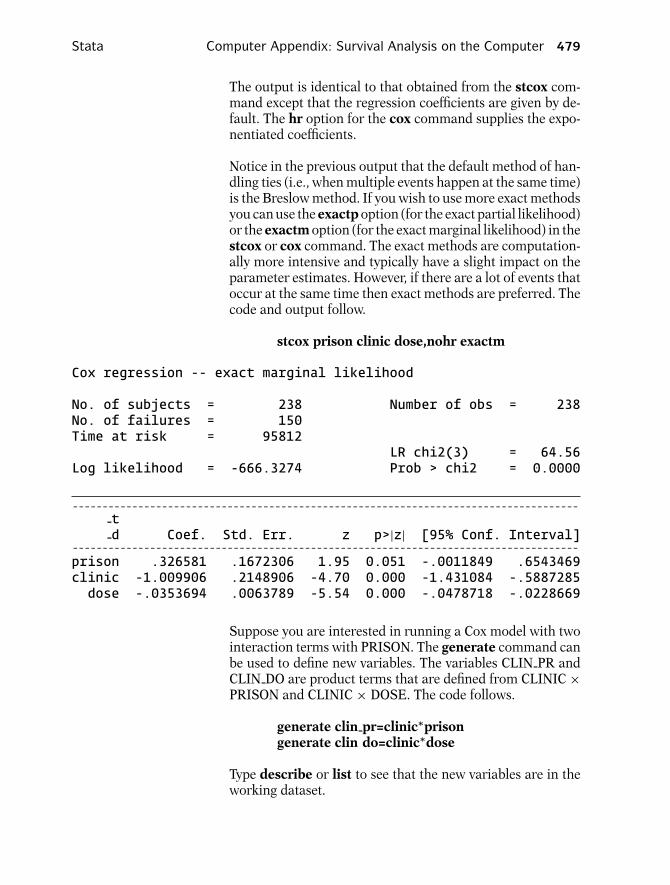
Stata Computer Appendix: Survival Analysis on the Computer 479
The output is identical to that obtained from the stcox com-mand except that the regression coefficients are given by de-fault. The hr option for the cox command supplies the expo-nentiated coefficients.
Notice in the previous output that the default method of han-dling ties (i.e., when multiple events happen at the same time)is the Breslow method. If you wish to use more exact methodsyou can use the exactp option (for the exact partial likelihood)or the exactm option (for the exact marginal likelihood) in thestcox or cox command. The exact methods are computation-ally more intensive and typically have a slight impact on theparameter estimates. However, if there are a lot of events thatoccur at the same time then exact methods are preferred. Thecode and output follow.
stcox prison clinic dose,nohr exactm
Cox regression -- exact marginal likelihood
No. of subjects = 238 Number of obs = 238No. of failures = 150Time at risk = 95812
LR chi2(3) = 64.56Log likelihood = -666.3274 Prob > chi2 = 0.0000
- - - - - - - - - - - - - - - - - - - - - - - - - - - - - - - - - - - - - - - - - - - - - - - - - - - - - - - - - - - - - - - - - - - - - - - - - - - - - - - - - - - - --t-d Coef. Std. Err. z p>|z| [95% Conf. Interval]
- - - - - - - - - - - - - - - - - - - - - - - - - - - - - - - - - - - - - - - - - - - - - - - - - - - - - - - - - - - - - - - - - - - - - - - - - - - - - - - - - - - - -prison .326581 .1672306 1.95 0.051 -.0011849 .6543469clinic -1.009906 .2148906 -4.70 0.000 -1.431084 -.5887285dose -.0353694 .0063789 -5.54 0.000 -.0478718 -.0228669
Suppose you are interested in running a Cox model with twointeraction terms with PRISON. The generate command canbe used to define new variables. The variables CLIN PR andCLIN DO are product terms that are defined from CLINIC ×PRISON and CLINIC × DOSE. The code follows.
generate clin pr=clinic∗prisongenerate clin do=clinic∗dose
Type describe or list to see that the new variables are in theworking dataset.

480 Computer Appendix: Survival Analysis on the Computer Stata
The following code runs the Cox model with the two interac-tion terms.
stcox prison clinic dose clin pr clin do, nohr
Cox regression -- Breslow method for ties
No. of subjects = 238 Number of obs = 238No. of failures = 150Time at risk = 95812
LR chi2(5) = 68.12Log likelihood = -671.59969 Prob > chi2 = 0.0000
- - - - - - - - - - - - - - - - - - - - - - - - - - - - - - - - - - - - - - - - - - - - - - - - - - - - - - - - - - - - - - - - - - - - - - - - - - - - - - - - - - - - --t-d Coef. Std. Err. z P>|z| [95% Conf. Interval]
- - - - - - - - - - - - - - - - - - - - - - - - - - - - - - - - - - - - - - - - - - - - - - - - - - - - - - - - - - - - - - - - - - - - - - - - - - - - - - - - - - - - -prison 1.191998 .5413685 2.20 0.028 .1309348 2.253061clinic .1746985 .893116 0.20 0.845 -1.575777 1.925174dose -.0193175 .01935 -1.00 0.318 -.0572428 .0186079
clin-pr -.7379931 .4314868 -1.71 0.087 -1.583692 .1077055clin-do -.0138608 .0143275 -0.97 0.333 -.0419422 .0142206
The lrtest command can be used to perform likelihood ratiotests. For example, to perform a likelihood ratio test on thetwo interaction terms CLIN PR and CLIN DO in the preced-ing model, we can save the −2 log likelihood statistic of thefull model in the computer’s memory by typing the followingcommand.
lrtest, saving(0)
Now the reduced model (without the interaction terms) canbe run (output omitted) by typing:
stcox prison clinic dose
After the reduced model is run, the following command pro-vides the results of the likelihood ratio test comparing the fullmodel (with the interaction terms) to the reduced model.
lrtest
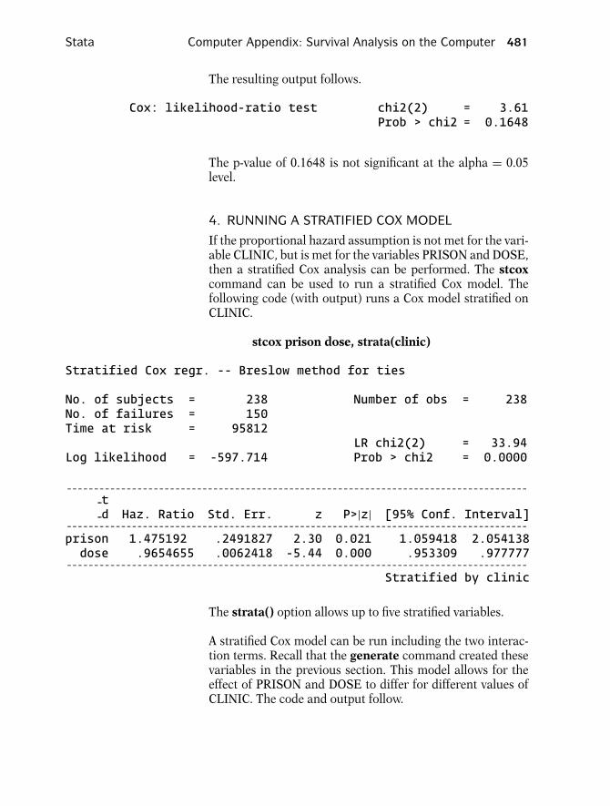
Stata Computer Appendix: Survival Analysis on the Computer 481
The resulting output follows.
Cox: likelihood-ratio test chi2(2) = 3.61Prob > chi2 = 0.1648
The p-value of 0.1648 is not significant at the alpha = 0.05level.
4. RUNNING A STRATIFIED COX MODEL
If the proportional hazard assumption is not met for the vari-able CLINIC, but is met for the variables PRISON and DOSE,then a stratified Cox analysis can be performed. The stcoxcommand can be used to run a stratified Cox model. Thefollowing code (with output) runs a Cox model stratified onCLINIC.
stcox prison dose, strata(clinic)
Stratified Cox regr. -- Breslow method for ties
No. of subjects = 238 Number of obs = 238No. of failures = 150Time at risk = 95812
LR chi2(2) = 33.94Log likelihood = -597.714 Prob > chi2 = 0.0000
- - - - - - - - - - - - - - - - - - - - - - - - - - - - - - - - - - - - - - - - - - - - - - - - - - - - - - - - - - - - - - - - - - - - - - - - - - - - - - - - - - - - --t-d Haz. Ratio Std. Err. z P>|z| [95% Conf. Interval]
- - - - - - - - - - - - - - - - - - - - - - - - - - - - - - - - - - - - - - - - - - - - - - - - - - - - - - - - - - - - - - - - - - - - - - - - - - - - - - - - - - - - -prison 1.475192 .2491827 2.30 0.021 1.059418 2.054138dose .9654655 .0062418 -5.44 0.000 .953309 .977777
- - - - - - - - - - - - - - - - - - - - - - - - - - - - - - - - - - - - - - - - - - - - - - - - - - - - - - - - - - - - - - - - - - - - - - - - - - - - - - - - - - - - -Stratified by clinic
The strata() option allows up to five stratified variables.
A stratified Cox model can be run including the two interac-tion terms. Recall that the generate command created thesevariables in the previous section. This model allows for theeffect of PRISON and DOSE to differ for different values ofCLINIC. The code and output follow.

482 Computer Appendix: Survival Analysis on the Computer Stata
stcox prison dose clin pr clin do, strata(clinic) nohr
Stratified Cox regr. -- Breslow method for ties
No. of subjects = 238 Number of obs = 238No. of failures = 150Time at risk = 95812
LR chi2(4) = 35.81Log likelihood = -596.77891 Prob > chi2 = 0.0000
- - - - - - - - - - - - - - - - - - - - - - - - - - - - - - - - - - - - - - - - - - - - - - - - - - - - - - - - - - - - - - - - - - - - - - - - - - - - - - - - - - - - --t-d Coef. Std. Err. z p>|z| [95% Conf. Interval]
- - - - - - - - - - - - - - - - - - - - - - - - - - - - - - - - - - - - - - - - - - - - - - - - - - - - - - - - - - - - - - - - - - - - - - - - - - - - - - - - - - - - -prison 1.087282 .5386163 2.02 0.044 .0316135 2.142951dose -.0348039 .0197969 -1.76 0.079 -.0736051 .0039973
clin-pr -.584771 .4281291 -1.37 0.172 -1.423889 .2543465clin-do -.0010622 .014569 -0.07 0.942 -.0296169 .0274925
Stratified by clinic
Suppose we wish to estimate the hazard ratio for PRISON =1 vs. PRISON = 0 for CLINIC = 2. This hazard ratio can beestimated by exponentiating the coefficient for prison plus2 times the coefficient for the clinic–prison interaction term.This expression is obtained by substituting the appropriatevalues into the hazard in both the numerator (for PRISON =1) and denominator (for PRISON = 0) (see below).
HR = h0(t) exp[1β1 + β2DOSE + (2)(1)β3 + β4CLIN DO]h0(t) exp[0β1 + β2DOSE + (2)(0)β3 + β4CLIN DO]
= exp(β1 + 2β3)
The lincom command can be used to exponentiate linearcombinations of parameters. Run this command directly af-ter running the model to estimate the HR for PRISON whereCLINIC = 2. The code and output follow.
lincom prison+2∗clin pr, hr
(1) prison + 2.0 clin-pr = 0.0- - - - - - - - - - - - - - - - - - - - - - - - - - - - - - - - - - - - - - - - - - - - - - - - - - - - - - - - - - - - - - - - - - - - - - - - - - - - - - - - - --t Haz. Ratio Std. Err. z p>|z| [95% Conf. Interval]
- - - - - - - - - - - - - - - - - - - - - - - - - - - - - - - - - - - - - - - - - - - - - - - - - - - - - - - - - - - - - - - - - - - - - - - - - - - - - - - - - -(1) .9210324 .3539571 -0.21 0.831 .4336648 1.956121- - - - - - - - - - - - - - - - - - - - - - - - - - - - - - - - - - - - - - - - - - - - - - - - - - - - - - - - - - - - - - - - - - - - - - - - - - - - - - - - - -

Stata Computer Appendix: Survival Analysis on the Computer 483
Models can also be run on a subset portion of the data usingthe if statement. The following code (with output) runs a Coxmodel on the data where CLINIC = 2.
stcox prison dose if clinic==2
Cox regression -- Breslow method for ties
No. of subjects = 75 Number of obs = 75No. of failures = 28Time at risk = 36254
LR chi2(2) = 9.70Log likelihood = -104.37135 Prob > chi2 = 0.0078
- - - - - - - - - - - - - - - - - - - - - - - - - - - - - - - - - - - - - - - - - - - - - - - - - - - - - - - - - - - - - - - - - - - - - - - - - - - - - - - - - - - - --t-d Haz. Ratio Std. Err. z p>|z| [95% Conf. Interval]
- - - - - - - - - - - - - - - - - - - - - - - - - - - - - - - - - - - - - - - - - - - - - - - - - - - - - - - - - - - - - - - - - - - - - - - - - - - - - - - - - - - - -prison .9210324 .3539571 -0.21 0.831 .4336648 1.956121dose .9637452 .0118962 -2.99 0.003 .9407088 .9873457
- - - - - - - - - - - - - - - - - - - - - - - - - - - - - - - - - - - - - - - - - - - - - - - - - - - - - - - - - - - - - - - - - - - - - - - - - - - - - - - - - - - - -
The hazard ratio estimates for PRISON = 1 vs. PRISON = 0(for CLINIC = 2) are exactly the same using the stratified Coxapproach with product terms and the subset data approach(0.9210324).
5. ASSESSING THE PH ASSUMPTION USINGA STATISTICAL TEST
The stphtest command can be used to perform a statisticaltest of the PH assumption. A statistical test gives objectivecriteria for assessing the PH assumption compared to usingthe graphical approach. This does not mean that this statisti-cal test is better than the graphical approach. It is just moreobjective. In fact, the graphical approach is generally moreinformative for descriptively characterizing the form of a PHviolation.
The command stphtest outputs a PH global test for all thecovariates simultaneously and can also be used to obtain atest for each covariate separately with the detail option. Torun these tests, you must obtain Schoenfeld residuals for theglobal test, and Schoenfeld scaled residuals for separate testswith each covariate. The idea behind the PH test is that ifthe PH assumption is satisfied, then the residuals should notbe correlated with survival time (or ranked survival time). Onthe other hand, if the residuals tend to be positive for subjectswho become events at a relatively early time and negativefor subjects who become events at a relatively late time (orvice versa), then there is evidence that the hazard ratio is notconstant over time (i.e., PH assumption is violated).

484 Computer Appendix: Survival Analysis on the Computer Stata
Before the stphtest can be implemented, the stcox com-mand needs to be run to obtain the Schoenfeld residuals(with the schoenfeld() option) and the scaled Schoenfeldresiduals (with the scaledsch() option). In the parenthesesare the names of newly defined variables; schoen∗ createsSCHOEN1, SCHOEN2, and SCHOEN3 whereas scaled∗ cre-ates SCALED1, SCALED2, and SCALED3. These variablescontain the residuals for PRISON, DOSE, and CLINIC, re-spectively (the order that the variables were entered in themodel). The user is free to type any variable name in the paren-theses. The Schoenfeld residuals are used for the global testand the scaled Schoenfeld residuals are used for the testingof the PH assumption for individual variables.
stcox prison dose clinic, schoenfeld(schoen∗) scaledsch(scaled∗)
Once the residuals are defined, the stphtest command can berun. The code and output follow.
stphtest, rank detail
Test of proportional hazards assumptionTime: Rank(t)- - - - - - - - - - - - - - - - - - - - - - - - - - - - - - - - - - - - - - - - - - - - - - - - - - - - - - - - -
rho chi2 df Prob>chi2- - - - - - - - - - - - - - - - - - - - - - - - - - - - - - - - - - - - - - - - - - - - - - - - - - - - - - - - -prison -0.04645 0.32 1 0.5689dose 0.08975 1.08 1 0.2996clinic -0.24927 10.44 1 0.0012- - - - - - - - - - - - - - - - - - - - - - - - - - - - - - - - - - - - - - - - - - - - - - - - - - - - - - - - -global test 12.36 3 0.0062- - - - - - - - - - - - - - - - - - - - - - - - - - - - - - - - - - - - - - - - - - - - - - - - - - - - - - - - -
The tests suggest that the PH assumption is violated forCLINIC with the p-value at 0.0012. The tests do not suggestviolation of the PH assumption for PRISON or DOSE.
The plot() option of the stphtest command can be used toproduce a plot of the scaled Schoenfeld residuals for CLINICagainst survival time ranking. If the PH assumption is met, thefitted curve should look horizontal because the scaled Schoen-feld residuals would be independent of survival time. The codeand graph follow.
stphtest,rank plot(clinic)

Stata Computer Appendix: Survival Analysis on the Computer 485
−5
0
5
scal
ed S
choe
nfe
ld-c
lin
ic
Test of PH Assumption
0 50 100 150
Rank(t)
The fitted curve slopes slightly downward (not horizontally).
6. OBTAINING COX ADJUSTED SURVIVAL CURVES
Adjusted survival curves can be obtained with the sts graphcommand. Adjusted survival curves depend on the patternof covariates. For example, the adjusted survival estimatesfor a subject with PRISON = 1, CLINIC = 1, and DOSE =40 are generally different than for a subject with PRISON =0, CLINIC = 2, and DOSE = 70. The sts graph commandproduces adjusted baseline survival curves. The followingcode produces an adjusted survival plot with PRISON = 0,CLINIC = 0, and DOSE = 0 (output omitted).
sts graph, adjustfor(prison dose clinic)
It is probably of more interest to create adjusted plots for rea-sonable patterns of covariates (CLINIC = 0 is not even a validvalue). Suppose we are interested in graphing the adjustedsurvival curve for PRISON = 0, CLINIC = 2, and DOSE =70. We can create new variables with the generate commandthat can be used with the sts graph command.
generate clinic2=clinic-2generate dose70=dose-70
These variables (PRISON, CLINIC2, and DOSE70) producethe desired pattern of covariate when each is set to zero. Thefollowing code produces the desired results.
sts graph, adjustfor(prison dose70 clinic2)

486 Computer Appendix: Survival Analysis on the Computer Stata
Survivor functionadjusted for prison dose70 clinic2
1.00
0.75
0.50
0.25
0.00
0 1000500
analysis time
Adjusted stratified Cox survival curves can be obtained withthe strata() option. The following code creates two survivalcurves stratified by clinic (CLINIC = 1, PRISON = 0, andDOSE = 70) and (CLINIC = 2, PRISON = 0, and DOSE =70).
sts graph, strata(clinic) adjustfor(prison dose70)
Survivor functions, by clinicadjusted for prison dose70
1.00
0.75
0.50
0.25
0.00
0 1000500
analysis time
clinic 2
clinic 1
The adjusted curves suggest there is a strong effect fromCLINIC on survival.

Stata Computer Appendix: Survival Analysis on the Computer 487
Suppose the interest is in comparing adjusted survival plotsof PRISON = 1 to PRISON = 0 stratified by CLINIC. In thissetting, the sts graph command cannot be used directly be-cause we cannot simultaneously define both levels of prison(PRISON = 1 and PRISON = 0) as the baseline level (recallsts graph plots only the baseline survival function). How-ever, survival estimates can be obtained using the sts gener-ate command twice; once where PRISON = 0 is defined asbaseline and once where PRISON = 1 is defined as baseline.The following code creates variables containing the desiredadjusted survival estimates.
generate prison1=prison-1sts generate scox0=s, strata(clinic) adjustfor(prison dose70)sts generate scox1=s, strata(clinic) adjustfor(prison1 dose70)
The variables SCOX1 and SCOX0 contain the survival esti-mates for PRISON = 1 and PRISON = 0, respectively, adjust-ing for dose and stratifying by clinic. The graph command isused to plot these estimates. If you are using a higher versionof Stata than Stata 7.0 (e.g., Stata 8.0), then you should re-place the graph command with the graph7 command. Thecode and output follow.
graph scox0 scox1 survt, twoway symbol([clinic] [clinic]) xlabel(365,730,1095)
1
.009935
365 730 1095
survival time in days
S(t+0), adjusted S(t+0), adjusted
We can also graph PRISON = 1 and PRISON = 0 with thedata subset where CLINIC = 1. The option twoway requestsa two-way scatterplot. The options symbol, xlabel, and titlerequest the symbols, axis labels, and title, respectively.

488 Computer Appendix: Survival Analysis on the Computer Stata
graph7 scox0 scox1 survt if clinic==1, twoway symbol(ox) xlabel(365,730,1095)t1(“symbols O for prison=0, × for prison=1”) title(“subsetted by clinic==1”)
1
.009935
365 730 1095
survival time in dayssubset by clinic==1
symbols O for prison=0, × for prison=1
7. RUNNING AN EXTENDED COX MODEL
If the PH assumption is not satisfied, a possible strategy is torun a stratified Cox model. Another strategy is to run a Coxmodel with time-varying covariates (an extended Cox model).The challenge of running an extended Cox model is to choosethe appropriate function of survival time to include in themodel.
Suppose we want to include a time-dependent covariateDOSE times the log of time. This product term could be appro-priate if the hazard ratio comparing any two levels of DOSEmonotonically increases (or decreases) over time. The tvc op-tion() of the stcox command can be used to declare DOSE atime-varying covariate that will be multiplied by a function oftime. The specification of that function of time is stated in thetexp option with the variable t representing time. The codeand output for a model containing the time-varying covariate,DOSE × ln( t), follow.

Stata Computer Appendix: Survival Analysis on the Computer 489
stcox prison clinic dose, tvc(dose) texp( ln( t)) nohr
Cox regression -- Breslow method for ties
No. of subjects = 238 Number of obs = 238No. of failures = 150Time at risk = 95812
LR chi2(4) = 66.29Log likelihood = -672.51694 Prob > chi2 = 0.0000- - - - - - - - - - - - - - - - - - - - - - - - - - - - - - - - - - - - - - - - - - - - - - - - - - - - - - - - - - - - - - - - - - - - - - - - - - - - - - - - - - - - -
-t-d Coef. Std. Err. z p>|z| [95% Conf. Interval]
- - - - - - - - - - - - - - - - - - - - - - - - - - - - - - - - - - - - - - - - - - - - - - - - - - - - - - - - - - - - - - - - - - - - - - - - - - - - - - - - - - - - -rh
prison .3404817 .1674672 2.03 0.042 .012252 .6687113clinic -1.018682 .215385 -4.73 0.000 -1.440829 -.5965352dose -.0824307 .0359866 -2.29 0.022 -.1529631 -.0118982
- - - - - - - - - - - - - - - - - - - - - - - - - - - - - - - - - - - - - - - - - - - - - - - - - - - - - - - - - - - - - - - - - - - - - - - - - - - - - - - - - - - - -t
dose .0085751 .0064554 1.33 0.184 -.0040772 .0212274- - - - - - - - - - - - - - - - - - - - - - - - - - - - - - - - - - - - - - - - - - - - - - - - - - - - - - - - - - - - - - - - - - - - - - - - - - - - - - - - - - - - -note: second equation contains variables that continuously vary
with respect to time; variables interact with currentvalues of ln(-t).
The parameter estimate for the time-dependent covariateDOSE × ln( t) is .0085751, however, it is not statistically sig-nificant with a Wald test p-value of 0.184.
A Heaviside function can also be used. The following coderuns a model with a time-dependent variable equal to CLINICif time is greater than or equal to 365 days and 0 other-wise.
stcox prison dose clinic, tvc(clinic) texp(-t >=365) nohr
Stata recognizes the expression ( t >= 365) as taking the value1 if survival time is ≥365 days and 0 otherwise. The outputfollows.

490 Computer Appendix: Survival Analysis on the Computer Stata
Cox regression -- Breslow method for ties
No. of subjects = 238 Number of obs = 238No. of failures = 150Time at risk = 95812
LR chi2(4) = 74.17Log likelihood = -668.57443 Prob > chi2 = 0.0000- - - - - - - - - - - - - - - - - - - - - - - - - - - - - - - - - - - - - - - - - - - - - - - - - - - - - - - - - - - - - - - - - - - - - - - - - - - - - - - - - - - - -
-t-d Coef. Std. Err. z p>|z| [95% Conf. Interval]
- - - - - - - - - - - - - - - - - - - - - - - - - - - - - - - - - - - - - - - - - - - - - - - - - - - - - - - - - - - - - - - - - - - - - - - - - - - - - - - - - - - - -rh
prison .377704 .1684024 2.24 0.025 .0476414 .7077666dose -.0355116 .0064354 -5.52 0.000 -.0481247 -.0228985
clinic -.4595628 .2552911 -1.80 0.072 -.959924 .0407985- - - - - - - - - - - - - - - - - - - - - - - - - - - - - - - - - - - - - - - - - - - - - - - - - - - - - - - - - - - - - - - - - - - - - - - - - - - - - - - - - - - - -t
clinic -1.368665 .4613948 -2.97 0.003 -2.272982 -.464348- - - - - - - - - - - - - - - - - - - - - - - - - - - - - - - - - - - - - - - - - - - - - - - - - - - - - - - - - - - - - - - - - - - - - - - - - - - - - - - - - - - - -note: second equation contains variables that continuously vary
with respect to time; variables interact with currentvalues of -t>=365.
Unfortunately, the texp option can only be used once in thestcox command. This makes it more difficult to run the equiv-alent model with two Heaviside functions. However, it can beaccomplished using the stsplit command, which adds extraobservations to the working dataset. The following code cre-ates a variable called V1 and adds new observations to thedataset.
stsplit v1, at(365)
After the above stsplit command is executed, any subject fol-lowed more than 365 days is represented by two observationsrather than one. For example, the first subject (ID = 1) hadan event on the 428th day; the first observation for that sub-ject shows no event between 0 and 365 days whereas the sec-ond observation shows an event on the 428th day. The newlydefined variable v1 has the value 365 for observations withsurvival time exceeding or equal to 365 and 0 otherwise. Thefollowing code lists the first 10 observations for the requestedvariables (output follows).

Stata Computer Appendix: Survival Analysis on the Computer 491
list id t0 t d clinic v1 in 1/10
id -t0 -t -d clinic v11. 1 0 365 0 1 02. 1 365 428 1 1 3653. 2 0 275 1 1 04. 3 0 262 1 1 05. 4 0 183 1 1 06. 5 0 259 1 1 07. 6 0 365 0 1 08. 6 365 714 1 1 3659. 7 0 365 0 1 010. 7 365 438 1 1 365
With the data in this form, two Heaviside functions can actu-ally be defined in the data using the following code.
generate hv2=clinic∗(v1/365)generate hv1=clinic∗(1-(v1/365))
The following code and output list a sample of the observa-tions (in 159/167) with the observation number suppressed(the noobs option).
list id t0 t clinic v1 hv1 hv2 in 159/167, noobs
id -t0 -t clinic v1 hv1 hv2100 0 365 1 0 1 0100 365 749 1 365 0 1101 0 150 1 0 1 0102 0 365 1 0 1 0102 365 465 1 365 0 1103 0 365 2 0 2 0103 365 708 2 365 0 2104 0 365 2 0 2 0104 365 713 2 365 0 2
With the two Heaviside functions defined in the split data, atime-dependent model using these functions can be run withthe following code (the output follows).

492 Computer Appendix: Survival Analysis on the Computer Stata
stcox prison clinic dose hv1 hv2, nohr
No. of subjects = 238 Number of obs = 360No. of failures = 150Time at risk = 95812
LR chi2(4) = 74.17Log likelihood = -668.57443 Prob > chi2 = 0.0000- - - - - - - - - - - - - - - - - - - - - - - - - - - - - - - - - - - - - - - - - - - - - - - - - - - - - - - - - - - - - - - - - - - - - - - - - - - - - - - - - - - - -
-t-d Coef. Std. Err. z p>|z| [95% Conf. Interval]
- - - - - - - - - - - - - - - - - - - - - - - - - - - - - - - - - - - - - - - - - - - - - - - - - - - - - - - - - - - - - - - - - - - - - - - - - - - - - - - - - - - - -prison .377704 .1684024 2.24 0.025 .0476414 .7077666dose -.0355116 .0064354 -5.52 0.000 -.0481247 -.0228985hv1 -.4595628 .2552911 -1.80 0.072 -.959924 .0407985hv2 -1.828228 .385946 -4.74 0.000 -2.584668 -1.071788
The stsplit command is complicated but it offers a powerfulapproach for manipulating the data to accommodate time-varying analyses.
If you wish to return the data to their previous form, drop thevariables that were created from the split and then use thestjoin command:
drop v1 hv1 hv2stjoin
It is possible to split the data at every single failure time, butthis uses a large amount of memory. However, if there is onlyone time-varying covariate in the model, the simplest wayto run an extended Cox model is by using the tvc and texpoptions with the stcox command.
One should not confuse an individual’s survival time variable(the outcome variable) with the variable used to define thetime-dependent variable ( t in Stata). The individual’s survivaltime variable is a time-independent variable. The time of theindividual’s event (or censorship) does not change. A time-dependent variable, on the other hand, is defined so that itcan change its values over time.
8. RUNNING PARAMETRIC MODELS
The Cox PH model is the most widely used model in survivalanalysis. A key reason why it is so popular is that the dis-tribution of the survival time variable need not be specified.However, if it is believed that survival time follows a partic-ular distribution, then that information can be utilized in aparametric modeling of survival data.

Stata Computer Appendix: Survival Analysis on the Computer 493
Many parametric models are accelerated failure time (AFT)models. Whereas the key assumption of a PH model is thathazard ratios are constant over time, the key assumption foran AFT model is that survival time accelerates (or deceler-ates) by a constant factor when comparing different levels ofcovariates.
The most common distribution for parametric modeling ofsurvival data is the Weibull distribution. The Weibull distri-bution has the desirable property that if the AFT assump-tion holds, then the PH assumption also holds. The exponen-tial distribution is a special case of the Weibull distribution.The key property for the exponential distribution is that thehazard is constant over time (not just the hazard ratio). TheWeibull and exponential model can be run as a PH model(the default) or an AFT model.
A graphical method for checking the validity of a Weibull as-sumption is to examine Kaplan–Meier log–log survival curvesagainst log survival time. This is accomplished with the stsgraph command (see Section 2 of this appendix). If the plotsare straight lines, then there is evidence that the distributionof survival times follows a Weibull distribution. If the slope ofthe line equals one, then the evidence suggests that survivaltime follows an exponential distribution.
The streg command is used to run parametric models. Eventhough the log–log survival curves obtained using the addictsdataset are not straight lines, the data are used for illustration.First a parametric model using the exponential distributionis demonstrated. The code and output follow.
streg prison dose clinic, dist(exponential) nohr
Exponential regression -- log relative-hazard form
No. of subjects = 238 Number of obs = 238No. of failures = 150Time at risk = 95812
LR chi2(3) = 49.91Log likelihood = -270.47929 Prob > chi2 = 0.0000
- - - - - - - - - - - - - - - - - - - - - - - - - - - - - - - - - - - - - - - - - - - - - - - - - - - - - - - - - - - - - - - - - - - - - - - - - - - - - - - - - - - - --t Coef. Std. Err. z p>|z| [95% Conf. Interval]
- - - - - - - - - - - - - - - - - - - - - - - - - - - - - - - - - - - - - - - - - - - - - - - - - - - - - - - - - - - - - - - - - - - - - - - - - - - - - - - - - - - - -prison .2526491 .1648862 1.53 0.125 -.070522 .5758201dose -.0289167 .0061445 -4.71 0.000 -.0409596 -.0168738
clinic -.8805819 .210626 -4.18 0.000 -1.293401 -.4677625-cons -3.684341 .4307163 -8.55 0.000 -4.528529 -2.840152
- - - - - - - - - - - - - - - - - - - - - - - - - - - - - - - - - - - - - - - - - - - - - - - - - - - - - - - - - - - - - - - - - - - - - - - - - - - - - - - - - - - - -
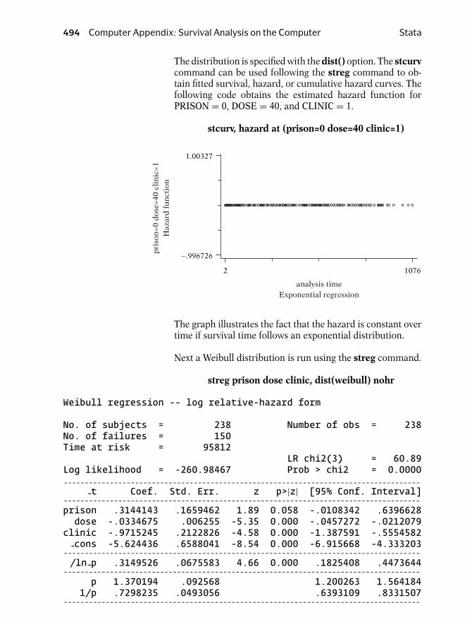
494 Computer Appendix: Survival Analysis on the Computer Stata
The distribution is specified with the dist() option. The stcurvcommand can be used following the streg command to ob-tain fitted survival, hazard, or cumulative hazard curves. Thefollowing code obtains the estimated hazard function forPRISON = 0, DOSE = 40, and CLINIC = 1.
stcurv, hazard at (prison=0 dose=40 clinic=1)
2 1076
analysis timeExponential regression
−.996726
1.00327p
riso
n=
0 d
ose=
40 c
lin
ic=
1H
azar
d f
un
ctio
n
The graph illustrates the fact that the hazard is constant overtime if survival time follows an exponential distribution.
Next a Weibull distribution is run using the streg command.
streg prison dose clinic, dist(weibull) nohr
Weibull regression -- log relative-hazard form
No. of subjects = 238 Number of obs = 238No. of failures = 150Time at risk = 95812
LR chi2(3) = 60.89Log likelihood = -260.98467 Prob > chi2 = 0.0000- - - - - - - - - - - - - - - - - - - - - - - - - - - - - - - - - - - - - - - - - - - - - - - - - - - - - - - - - - - - - - - - - - - - - - - - - - - - - - - - - - - - -
-t Coef. Std. Err. z p>|z| [95% Conf. Interval]- - - - - - - - - - - - - - - - - - - - - - - - - - - - - - - - - - - - - - - - - - - - - - - - - - - - - - - - - - - - - - - - - - - - - - - - - - - - - - - - - - - - -prison .3144143 .1659462 1.89 0.058 -.0108342 .6396628dose -.0334675 .006255 -5.35 0.000 -.0457272 -.0212079
clinic -.9715245 .2122826 -4.58 0.000 -1.387591 -.5554582-cons -5.624436 .6588041 -8.54 0.000 -6.915668 -4.333203
- - - - - - - - - - - - - - - - - - - - - - - - - - - - - - - - - - - - - - - - - - - - - - - - - - - - - - - - - - - - - - - - - - - - - - - - - - - - - - - - - - - - -/ln-p .3149526 .0675583 4.66 0.000 .1825408 .4473644
- - - - - - - - - - - - - - - - - - - - - - - - - - - - - - - - - - - - - - - - - - - - - - - - - - - - - - - - - - - - - - - - - - - - - - - - - - - - - - - - - - - - -p 1.370194 .092568 1.200263 1.564184
1/p .7298235 .0493056 .6393109 .8331507- - - - - - - - - - - - - - - - - - - - - - - - - - - - - - - - - - - - - - - - - - - - - - - - - - - - - - - - - - - - - - - - - - - - - - - - - - - - - - - - - - - - -
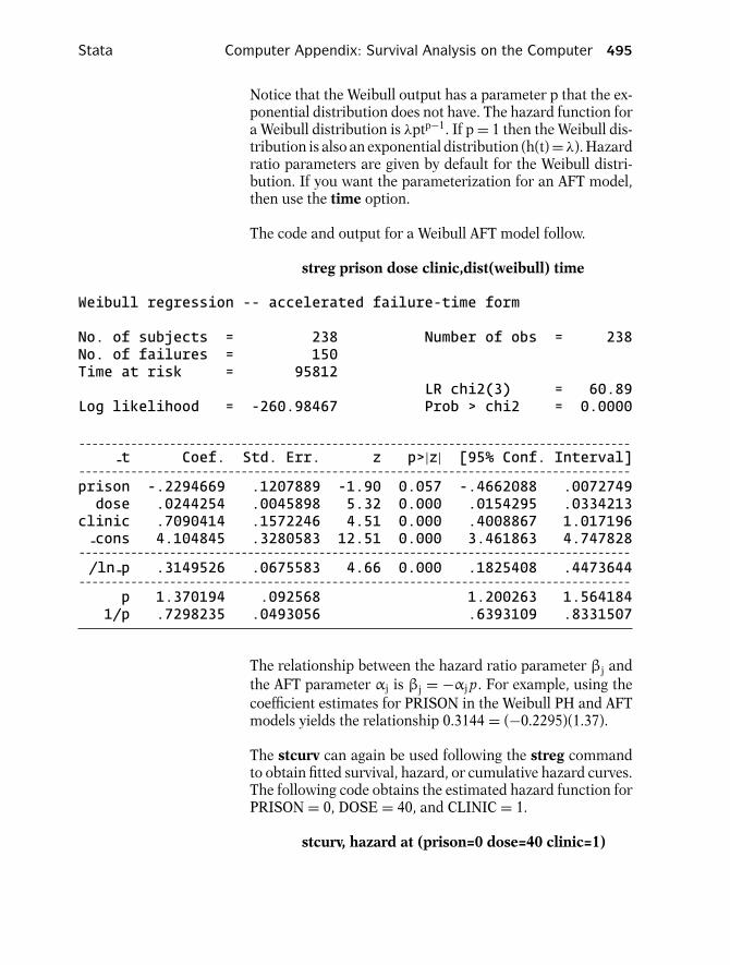
Stata Computer Appendix: Survival Analysis on the Computer 495
Notice that the Weibull output has a parameter p that the ex-ponential distribution does not have. The hazard function fora Weibull distribution is λptp−1. If p = 1 then the Weibull dis-tribution is also an exponential distribution (h(t) =λ). Hazardratio parameters are given by default for the Weibull distri-bution. If you want the parameterization for an AFT model,then use the time option.
The code and output for a Weibull AFT model follow.
streg prison dose clinic,dist(weibull) time
Weibull regression -- accelerated failure-time form
No. of subjects = 238 Number of obs = 238No. of failures = 150Time at risk = 95812
LR chi2(3) = 60.89Log likelihood = -260.98467 Prob > chi2 = 0.0000
- - - - - - - - - - - - - - - - - - - - - - - - - - - - - - - - - - - - - - - - - - - - - - - - - - - - - - - - - - - - - - - - - - - - - - - - - - - - - - - - - - - - --t Coef. Std. Err. z p>|z| [95% Conf. Interval]
- - - - - - - - - - - - - - - - - - - - - - - - - - - - - - - - - - - - - - - - - - - - - - - - - - - - - - - - - - - - - - - - - - - - - - - - - - - - - - - - - - - - -prison -.2294669 .1207889 -1.90 0.057 -.4662088 .0072749dose .0244254 .0045898 5.32 0.000 .0154295 .0334213
clinic .7090414 .1572246 4.51 0.000 .4008867 1.017196-cons 4.104845 .3280583 12.51 0.000 3.461863 4.747828
- - - - - - - - - - - - - - - - - - - - - - - - - - - - - - - - - - - - - - - - - - - - - - - - - - - - - - - - - - - - - - - - - - - - - - - - - - - - - - - - - - - - -/ln-p .3149526 .0675583 4.66 0.000 .1825408 .4473644
- - - - - - - - - - - - - - - - - - - - - - - - - - - - - - - - - - - - - - - - - - - - - - - - - - - - - - - - - - - - - - - - - - - - - - - - - - - - - - - - - - - - -p 1.370194 .092568 1.200263 1.564184
1/p .7298235 .0493056 .6393109 .8331507
The relationship between the hazard ratio parameter βj andthe AFT parameter αj is βj = −αj p. For example, using thecoefficient estimates for PRISON in the Weibull PH and AFTmodels yields the relationship 0.3144 = (−0.2295)(1.37).
The stcurv can again be used following the streg commandto obtain fitted survival, hazard, or cumulative hazard curves.The following code obtains the estimated hazard function forPRISON = 0, DOSE = 40, and CLINIC = 1.
stcurv, hazard at (prison=0 dose=40 clinic=1)
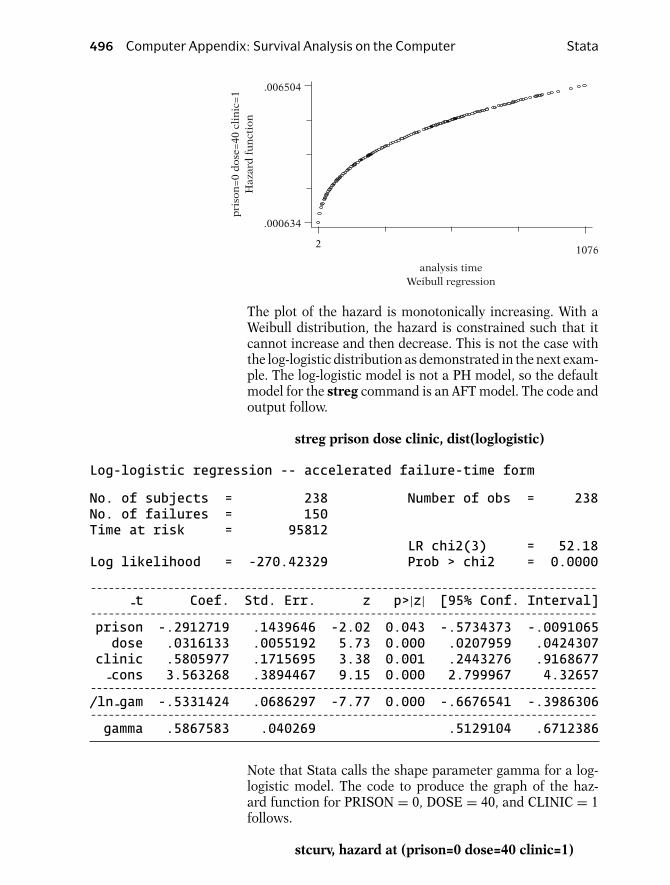
496 Computer Appendix: Survival Analysis on the Computer Stata
.006504
.000634p
riso
n=
0 d
ose=
40 c
lin
ic=
1H
azar
d f
un
ctio
n2
1076
analysis timeWeibull regression
The plot of the hazard is monotonically increasing. With aWeibull distribution, the hazard is constrained such that itcannot increase and then decrease. This is not the case withthe log-logistic distribution as demonstrated in the next exam-ple. The log-logistic model is not a PH model, so the defaultmodel for the streg command is an AFT model. The code andoutput follow.
streg prison dose clinic, dist(loglogistic)
Log-logistic regression -- accelerated failure-time form
No. of subjects = 238 Number of obs = 238No. of failures = 150Time at risk = 95812
LR chi2(3) = 52.18Log likelihood = -270.42329 Prob > chi2 = 0.0000
- - - - - - - - - - - - - - - - - - - - - - - - - - - - - - - - - - - - - - - - - - - - - - - - - - - - - - - - - - - - - - - - - - - - - - - - - - - - - - - - - - - - --t Coef. Std. Err. z p>|z| [95% Conf. Interval]
- - - - - - - - - - - - - - - - - - - - - - - - - - - - - - - - - - - - - - - - - - - - - - - - - - - - - - - - - - - - - - - - - - - - - - - - - - - - - - - - - - - - -prison -.2912719 .1439646 -2.02 0.043 -.5734373 -.0091065dose .0316133 .0055192 5.73 0.000 .0207959 .0424307
clinic .5805977 .1715695 3.38 0.001 .2443276 .9168677-cons 3.563268 .3894467 9.15 0.000 2.799967 4.32657
- - - - - - - - - - - - - - - - - - - - - - - - - - - - - - - - - - - - - - - - - - - - - - - - - - - - - - - - - - - - - - - - - - - - - - - - - - - - - - - - - - - - -/ln-gam -.5331424 .0686297 -7.77 0.000 -.6676541 -.3986306- - - - - - - - - - - - - - - - - - - - - - - - - - - - - - - - - - - - - - - - - - - - - - - - - - - - - - - - - - - - - - - - - - - - - - - - - - - - - - - - - - - - -gamma .5867583 .040269 .5129104 .6712386
Note that Stata calls the shape parameter gamma for a log-logistic model. The code to produce the graph of the haz-ard function for PRISON = 0, DOSE = 40, and CLINIC = 1follows.
stcurv, hazard at (prison=0 dose=40 clinic=1)

Stata Computer Appendix: Survival Analysis on the Computer 497
2 1076
.000809
.007292
analysis timeLog-logistic regression
pri
son
=0
dos
e=20
cli
nic
=1
Haz
ard
fu
nct
ion
The hazard function (in contrast to the Weibull hazard func-tion) first increases and then decreases.
The corresponding survival curve for the log-logistic distribu-tion can also be obtained with the stcurve command.
stcurv, survival at (prison=0 dose=40 clinic=1)
2 1076
.064154
.999677
analysis timeLog-logistic regression
pri
son
=0
dos
e=40
cli
nic
=1
Su
rviv
al
If the AFT assumption holds for a log-logistic model, then theproportional odds assumption holds for the survival function(although the PH assumption would not hold). The propor-tional odds assumption can be evaluated by plotting the logodds of survival (using KM estimates) against the log of sur-vival time. If the plots are straight lines for each pattern ofcovariates, then the log-logistic distribution is reasonable. Ifthe straight lines are also parallel, then the proportional oddsand AFT assumptions also hold. The following code will plotthe estimated log odds of survival against the log of time byCLINIC (output omitted).

498 Computer Appendix: Survival Analysis on the Computer Stata
sts generate skm=s,by (clinic)generate logodds=ln(skm/(1-skm))generate logt=ln(survt)graph7 logodds logt,twoway symbol([clinic] [clinic])
Another context for thinking about the proportional odds as-sumption is that the odds ratio estimated by a logistic re-gression does not depend on the length of the follow-up. Forexample, if a follow-up study was extended from three to fiveyears then the underlying odds ratio comparing two patternsof covariates would not change. If the proportional odds as-sumption is not true, then the odds ratio is specific to thelength of follow-up.
Both the log-logistic and Weibull models contain an extrashape parameter that is typically assumed constant. This as-sumption is necessary for the PH or AFT assumption to holdfor these models. Stata provides a way of modeling the shapeparameter as a function of predictor variables by use of theancillary option in the streg command (see Chapter 7 un-der the heading, “Other Parametric Models”). The followingcode runs a log-logistic model in which the shape parametergamma is modeled as a function of CLINIC and λ is modeledas a function of PRISON and DOSE.
streg prison dose, dist(loglogistic) ancillary(clinic)
The output follows.
Log-logistic regression -- accelerated failure-time form
No. of subjects = 238 Number of obs = 238No. of failures = 150Time at risk = 95812
LR chi2(2) = 38.87Log likelihood = -272.65273 Prob > chi2 = 0.0000
- - - - - - - - - - - - - - - - - - - - - - - - - - - - - - - - - - - - - - - - - - - - - - - - - - - - - - - - - - - - - - - - - - - - - - - - - - - - - - - - - - - - - - - - - - - --t Coef. Std. Err. z p>|z| [95% Conf. Interval]
- - - - - - - - - - - - - - - - - - - - - - - - - - - - - - - - - - - - - - - - - - - - - - - - - - - - - - - - - - - - - - - - - - - - - - - - - - - - - - - - - - - - - - - - - - - -
-tprison -.3275695 .1405119 -2.33 0.020 -.6029677 -.0521713dose .0328517 .0054275 6.05 0.000 .022214 .0434893-cons 4.183173 .3311064 12.63 0.000 3.534216 4.83213
- - - - - - - - - - - - - - - - - - - - - - - - - - - - - - - - - - - - - - - - - - - - - - - - - - - - - - - - - - - - - - - - - - - - - - - - - - - - - - - - - - - - - - - - - - - -ln-gam
clinic .4558089 .1734819 2.63 0.009 .1157906 .7958273-cons -1.094496 .2212143 -4.95 0.000 -1.528068 -.6609238
- - - - - - - - - - - - - - - - - - - - - - - - - - - - - - - - - - - - - - - - - - - - - - - - - - - - - - - - - - - - - - - - - - - - - - - - - - - - - - - - - - - - - - - - - - - -
Stata Computer Appendix: Survival Analysis on the Computer 499
Notice there is a parameter estimate for CLINIC as well asan intercept ( cons) under the heading ln gam (the log ofgamma). With this model, the estimate for gamma depends onwhether CLINIC = 1 or CLINIC = 2. There is no easy interpre-tation for the predictor variables in this type of model, whichis why it is not commonly used. However, for any specifiedvalue of PRISON, DOSE, and CLINIC, the hazard and sur-vival functions can be estimated by substituting the parame-ter estimates into the expressions for the log-logistic hazardand survival functions.
Other distributions supported by streg are the generalizedgamma, the lognormal, and the Gompertz distributions.
9. RUNNING FRAILTY MODELS
Frailty models contain an extra random component designedto account for individual level differences in the hazard oth-erwise unaccounted for by the model. The frailty α is a multi-plicative effect on the hazard assumed to follow some distri-bution. The hazard function conditional on the frailty can beexpressed as h(t|α) = α[h(t)].
Stata offers two choices for the distribution of the frailty: thegamma and the inverse-Gaussian, both of mean 1 and vari-ance theta. The variance (theta) is a parameter estimated bythe model. If theta = 0, then there is no frailty.
For the first example, a Weibull PH model is run withPRISON, DOSE, and CLINIC as predictors. A gamma dis-tribution is assumed for the frailty component. The codefollows.
streg dose prison clinic, dist(weibull) frailty(gamma) nohr
The frailty() option requests that a frailty model be run. Theoutput follows.

500 Computer Appendix: Survival Analysis on the Computer Stata
Weibull regression -- log relative-hazard formGamma frailty
No. of subjects = 238 Number of obs = 238No. of failures = 150Time at risk = 95812
LR chi2(4) = 60.89Log likelihood = -260.98467 Prob > chi2 = 0.0000- - - - - - - - - - - - - - - - - - - - - - - - - - - - - - - - - - - - - - - - - - - - - - - - - - - - - - - - - - - - - - - - - - - - - - - - - - - - - - - - - - - - -
-t Coef. Std. Err. z p>|z| [95% Conf. Interval]- - - - - - - - - - - - - - - - - - - - - - - - - - - - - - - - - - - - - - - - - - - - - - - - - - - - - - - - - - - - - - - - - - - - - - - - - - - - - - - - - - - - -dose -.0334635 .0062553 -5.35 0.000 -.0457237 -.0212034
prison .3143786 .165953 1.89 0.058 -.0108833 .6396405clinic -.9714998 .2122909 -4.58 0.000 -1.387582 -.5554173-cons -5.624342 .6588994 -8.54 0.000 -6.915761 -4.332923
- - - - - - - - - - - - - - - - - - - - - - - - - - - - - - - - - - - - - - - - - - - - - - - - - - - - - - - - - - - - - - - - - - - - - - - - - - - - - - - - - - - - -/ln-p .3149036 .0675772 4.66 0.000 .1824548 .4473525
/ln-the -15.37947 722.4246 -0.02 0.983 -1431.306 1400.547- - - - - - - - - - - - - - - - - - - - - - - - - - - - - - - - - - - - - - - - - - - - - - - - - - - - - - - - - - - - - - - - - - - - - - - - - - - - - - - - - - - - -
p 1.370127 .0925893 1.20016 1.5641661/p .7298592 .0493218 .6393185 .8332223
theta 2.09e-07 .0001512 0 .- - - - - - - - - - - - - - - - - - - - - - - - - - - - - - - - - - - - - - - - - - - - - - - - - - - - - - - - - - - - - - - - - - - - - - - - - - - - - - - - - - - - -Likelihood ratio test of theta = 0: chibar2(01) = 0.00Prob>=chibar2 = 1.000
Notice that there is one additional parameter (theta) com-pared to the model run in the previous section. The estimatefor theta is 2.09 times 10−7 or 0.000000209 which is essen-tially zero. A likelihood ratio test for the inclusion of theta isprovided at the bottom of the output and yields a chi-squarevalue of 0.00 and a p-value of 1.000. The frailty has no effecton the model and need not be included.
The next model is the same as the previous one except thatCLINIC is not included. One might expect a frailty componentto play a larger role if an important covariate, such as CLINIC,is not included in the model. The code and output follow.

Stata Computer Appendix: Survival Analysis on the Computer 501
streg dose prison, dist(weibull) frailty(gamma) nohr
Weibull regression -- log relative-hazard formGamma frailty
No. of subjects = 238 Number of obs = 238No. of failures = 150Time at risk = 95812
LR chi2(3) = 36.00Log likelihood = -273.42782 Prob > chi2 = 0.0000- - - - - - - - - - - - - - - - - - - - - - - - - - - - - - - - - - - - - - - - - - - - - - - - - - - - - - - - - - - - - - - - - - - - - - - - - - - - - - - - - - - - -
-t Coef. Std. Err. z p>|z| [95% Conf. Interval]- - - - - - - - - - - - - - - - - - - - - - - - - - - - - - - - - - - - - - - - - - - - - - - - - - - - - - - - - - - - - - - - - - - - - - - - - - - - - - - - - - - - -dose -.0358231 .010734 -3.34 0.001 -.0568614 -.0147849
prison .2234556 .2141028 1.04 0.297 -.1961783 .6430894-cons -6.457393 .6558594 -9.85 0.000 -7.742854 -5.171932
- - - - - - - - - - - - - - - - - - - - - - - - - - - - - - - - - - - - - - - - - - - - - - - - - - - - - - - - - - - - - - - - - - - - - - - - - - - - - - - - - - - - -/ln-p .2922832 .1217597 2.40 0.016 .0536385 .5309278
/ln-the -2.849726 5.880123 -0.48 0.628 -14.37456 8.675104- - - - - - - - - - - - - - - - - - - - - - - - - - - - - - - - - - - - - - - - - - - - - - - - - - - - - - - - - - - - - - - - - - - - - - - - - - - - - - - - - - - - -
p 1.339482 .163095 1.055103 1.7005091/p .7465571 .0909006 .5880591 .9477747
theta .0578602 .340225 5.72e-07 5855.31- - - - - - - - - - - - - - - - - - - - - - - - - - - - - - - - - - - - - - - - - - - - - - - - - - - - - - - - - - - - - - - - - - - - - - - - - - - - - - - - - - - - -Likelihood ratio test of theta = 0: chibar2(01) = 0.03Prob>=chibar2 = 0.432
The variance (theta) of the frailty is estimated at 0.0578602.Although this estimate is not exactly zero as in the previousexample, the p-value for the likelihood ratio test for theta isnonsignificant at 0.432. So the addition of frailty did not ac-count for CLINIC being omitted from the model.
Next the same model is run except that the inverse-Gaussiandistribution is used for the frailty rather than the gamma dis-tribution. The code and output follow.
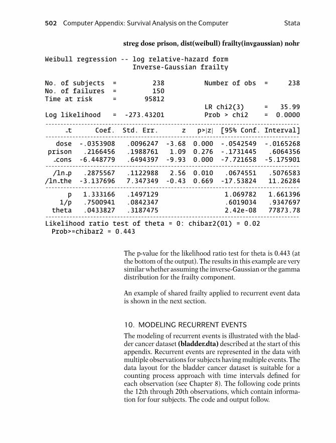
502 Computer Appendix: Survival Analysis on the Computer Stata
streg dose prison, dist(weibull) frailty(invgaussian) nohr
Weibull regression -- log relative-hazard formInverse-Gaussian frailty
No. of subjects = 238 Number of obs = 238No. of failures = 150Time at risk = 95812
LR chi2(3) = 35.99Log likelihood = -273.43201 Prob > chi2 = 0.0000- - - - - - - - - - - - - - - - - - - - - - - - - - - - - - - - - - - - - - - - - - - - - - - - - - - - - - - - - - - - - - - - - - - - - - - - - - - - - - - - - - - - -
-t Coef. Std. Err. z p>|z| [95% Conf. Interval]- - - - - - - - - - - - - - - - - - - - - - - - - - - - - - - - - - - - - - - - - - - - - - - - - - - - - - - - - - - - - - - - - - - - - - - - - - - - - - - - - - - - -dose -.0353908 .0096247 -3.68 0.000 -.0542549 -.0165268
prison .2166456 .1988761 1.09 0.276 -.1731445 .6064356-cons -6.448779 .6494397 -9.93 0.000 -7.721658 -5.175901
- - - - - - - - - - - - - - - - - - - - - - - - - - - - - - - - - - - - - - - - - - - - - - - - - - - - - - - - - - - - - - - - - - - - - - - - - - - - - - - - - - - - -/ln-p .2875567 .1122988 2.56 0.010 .0674551 .5076583
/ln-the -3.137696 7.347349 -0.43 0.669 -17.53824 11.26284- - - - - - - - - - - - - - - - - - - - - - - - - - - - - - - - - - - - - - - - - - - - - - - - - - - - - - - - - - - - - - - - - - - - - - - - - - - - - - - - - - - - -
p 1.333166 .1497129 1.069782 1.6613961/p .7500941 .0842347 .6019034 .9347697
theta .0433827 .3187475 2.42e-08 77873.78- - - - - - - - - - - - - - - - - - - - - - - - - - - - - - - - - - - - - - - - - - - - - - - - - - - - - - - - - - - - - - - - - - - - - - - - - - - - - - - - - - - - -Likelihood ratio test of theta = 0: chibar2(01) = 0.02Prob>=chibar2 = 0.443
The p-value for the likelihood ratio test for theta is 0.443 (atthe bottom of the output). The results in this example are verysimilar whether assuming the inverse-Gaussian or the gammadistribution for the frailty component.
An example of shared frailty applied to recurrent event datais shown in the next section.
10. MODELING RECURRENT EVENTS
The modeling of recurrent events is illustrated with the blad-der cancer dataset (bladder.dta) described at the start of thisappendix. Recurrent events are represented in the data withmultiple observations for subjects having multiple events. Thedata layout for the bladder cancer dataset is suitable for acounting process approach with time intervals defined foreach observation (see Chapter 8). The following code printsthe 12th through 20th observations, which contain informa-tion for four subjects. The code and output follow.

Stata Computer Appendix: Survival Analysis on the Computer 503
list in 12/20
id event interval start stop tx num size12. 10 1 1 0 12 0 1 113. 10 1 2 12 16 0 1 114. 10 0 3 16 18 0 1 115. 11 0 1 0 23 0 3 316. 12 1 1 0 10 0 1 317. 12 1 2 10 15 0 1 318. 12 0 3 15 23 0 1 319. 13 1 1 0 3 0 1 120. 13 1 2 3 16 0 1 1
There are three observations for ID = 10, one observation forID = 11, three observations for ID = 12, and two observationsfor ID = 13. The variables START and STOP represent thetime interval for the risk period specific to that observation.The variable EVENT indicates whether an event (coded 1)occurred. The first three observations indicate that the subjectwith ID = 10 had an event at 12 months, another event at 16months, and was censored at 18 months.
Before using Stata’s survival commands, the stset commandmust be used to define the key survival variables. The codefollows.
stset stop, failure(event==1) id(id) time0(start) exit(time .)
We have previously used the stset command on the addictsdataset, but more options from stset are included here. Theid() option defines the subject variable (i.e., the cluster vari-able), the time0() option defines the variable that begins thetime interval, and the exit(time .) option tells Stata that thereis no imposed limit on the length of follow-up time for a givensubject (e.g., subjects are not out of the risk set after theirfirst event). With the stset command, Stata creates the vari-ables t0, t, and d, which Stata automatically recognizesas survival variables representing the time interval and eventstatus. Actually the time0( ) option could have been omittedfrom this stset command and by default Stata would havecreated the starting time variable t0 in the correct countingprocess format as long as the id() option was used (otherwiset0 would default to zero). The following code (and output)
lists the 12th through 20th observation with the newly createdvariables.
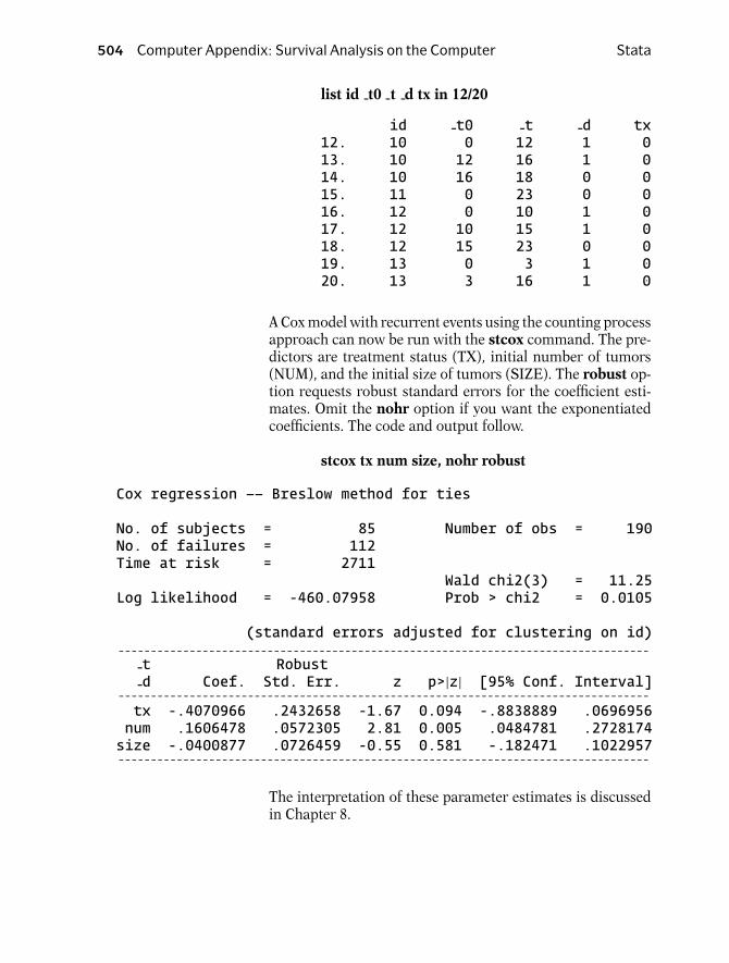
504 Computer Appendix: Survival Analysis on the Computer Stata
list id t0 t d tx in 12/20
id -t0 -t -d tx12. 10 0 12 1 013. 10 12 16 1 014. 10 16 18 0 015. 11 0 23 0 016. 12 0 10 1 017. 12 10 15 1 018. 12 15 23 0 019. 13 0 3 1 020. 13 3 16 1 0
A Cox model with recurrent events using the counting processapproach can now be run with the stcox command. The pre-dictors are treatment status (TX), initial number of tumors(NUM), and the initial size of tumors (SIZE). The robust op-tion requests robust standard errors for the coefficient esti-mates. Omit the nohr option if you want the exponentiatedcoefficients. The code and output follow.
stcox tx num size, nohr robust
Cox regression –– Breslow method for ties
No. of subjects = 85 Number of obs = 190No. of failures = 112Time at risk = 2711
Wald chi2(3) = 11.25Log likelihood = -460.07958 Prob > chi2 = 0.0105
(standard errors adjusted for clustering on id)- - - - - - - - - - - - - - - - - - - - - - - - - - - - - - - - - - - - - - - - - - - - - - - - - - - - - - - - - - - - - - - - - - - - - - - - - - - - - - - - - --t Robust-d Coef. Std. Err. z p>|z| [95% Conf. Interval]
- - - - - - - - - - - - - - - - - - - - - - - - - - - - - - - - - - - - - - - - - - - - - - - - - - - - - - - - - - - - - - - - - - - - - - - - - - - - - - - - - -tx -.4070966 .2432658 -1.67 0.094 -.8838889 .0696956num .1606478 .0572305 2.81 0.005 .0484781 .2728174size -.0400877 .0726459 -0.55 0.581 -.182471 .1022957- - - - - - - - - - - - - - - - - - - - - - - - - - - - - - - - - - - - - - - - - - - - - - - - - - - - - - - - - - - - - - - - - - - - - - - - - - - - - - - - - -
The interpretation of these parameter estimates is discussedin Chapter 8.

Stata Computer Appendix: Survival Analysis on the Computer 505
A stratified Cox model can also be run using the data in thisformat with the variable INTERVAL as the stratified variable.The stratified variable indicates whether subjects were at riskfor their 1st, 2nd, 3rd, or 4th event. This approach is calledconditional 1 in Chapter 8 and is used if the investigatorwants to distinguish the order in which recurrent events oc-cur. The code and output follow.
stcox tx num size, nohr robust strata(interval)
stratified Cox regr. –– Breslow method for ties
No. of subjects = 85 Number of obs = 190No. of failures = 112Time at risk = 2711
Wald chi2(3) = 7.11Log likelihood = -319.85912 Prob > chi2 = 0.0685
(standard errors adjusted for clustering on id)- - - - - - - - - - - - - - - - - - - - - - - - - - - - - - - - - - - - - - - - - - - - - - - - - - - - - - - - - - - - - - - - - - - - - - - - - - - - - - - - - --t Robust-d Coef. Std. Err. z p>|z| [95% Conf. Interval]
- - - - - - - - - - - - - - - - - - - - - - - - - - - - - - - - - - - - - - - - - - - - - - - - - - - - - - - - - - - - - - - - - - - - - - - - - - - - - - - - - -tx -.3342955 .1982339 -1.69 0.092 -.7228268 .0542359num .1156526 .0502089 2.30 0.021 .017245 .2140603size -.0080508 .0604807 -0.13 0.894 -.1265908 .1104892- - - - - - - - - - - - - - - - - - - - - - - - - - - - - - - - - - - - - - - - - - - - - - - - - - - - - - - - - - - - - - - - - - - - - - - - - - - - - - - - - -
Stratified by interval
Interaction terms between the treatment variable (TX) andthe stratified variable could be created to examine whetherthe effect of treatment differed for the 1st, 2nd, 3rd, or 4thevent. (Note that in this dataset subjects have a maximum of4 events).
Another stratified approach (called conditional 2) is a slightvariation of the conditional 1 approach. The difference is inthe way the time intervals for the recurrent events are defined.There is no difference in the time intervals when subjects areat risk for their first event. However, with the conditional 2approach, the starting time at risk gets reset to zero for eachsubsequent event. The following code creates data suitablefor using the conditional 2 approach.
generate stop2 = t - t0stset stop2, failure(event==1) exit(time .)

506 Computer Appendix: Survival Analysis on the Computer Stata
The generate command defines a new variable called STOP2representing the length of the time interval for each observa-tion. The stset command is used with STOP2 as the outcomevariable ( t). By default Stata sets the variable t0 to zero.The following code (and output) lists the 12th through 20thobservations for selected variables.
list id t0 t d tx in 12/20
id -t0 -t -d tx12. 10 0 12 1 013. 10 0 4 1 014. 10 0 2 0 015. 11 0 23 0 016. 12 0 10 1 017. 12 0 5 1 018. 12 0 8 0 019. 13 0 3 1 020. 13 0 13 1 0
Notice that the id() option was not used with the stset com-mand for the conditional 2 approach. This means that Statadoes not know that multiple observations correspond to thesame subject. However the cluster() option can be used di-rectly in the stcox command to request that the analysis beclustered by ID (i.e., by subject). The following code runs astratified Cox model using the conditional 2 approach with thecluster() and robust options. The code and output follow.
stcox tx num size, nohr robust strata(interval) cluster(id)
Stratified Cox regr. –– Breslow method for ties
No. of subjects = 190 Number of obs = 190No. of failures = 112Time at risk = 2711
Wald chi2(3) = 11.99Log likelihood = -363.16022 Prob > chi2 = 0.0074
(standard errors adjusted for clustering on id)- - - - - - - - - - - - - - - - - - - - - - - - - - - - - - - - - - - - - - - - - - - - - - - - - - - - - - - - - - - - - - - - - - - - - - - - - - - - - - - - - --t Robust-d Coef. Std. Err. z p>|z| [95% Conf. Interval]
- - - - - - - - - - - - - - - - - - - - - - - - - - - - - - - - - - - - - - - - - - - - - - - - - - - - - - - - - - - - - - - - - - - - - - - - - - - - - - - - - -tx -.2695213 .2093108 -1.29 0.198 -.6797628 .1407203num .1535334 .0491803 3.12 0.002 .0571418 .2499249size .0068402 .0625862 0.11 0.913 -.1158265 .129507- - - - - - - - - - - - - - - - - - - - - - - - - - - - - - - - - - - - - - - - - - - - - - - - - - - - - - - - - - - - - - - - - - - - - - - - - - - - - - - - - -
Stratified by interval
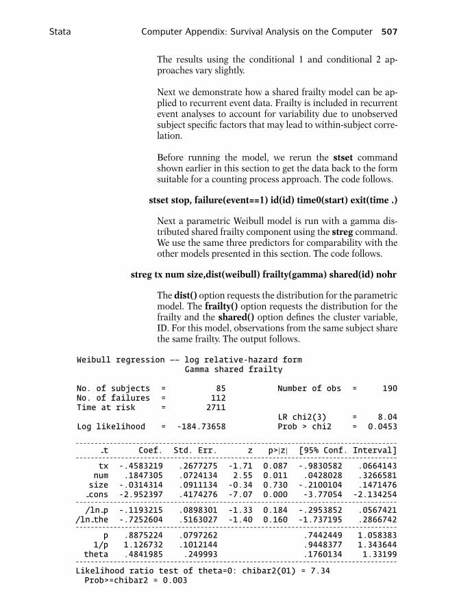
Stata Computer Appendix: Survival Analysis on the Computer 507
The results using the conditional 1 and conditional 2 ap-proaches vary slightly.
Next we demonstrate how a shared frailty model can be ap-plied to recurrent event data. Frailty is included in recurrentevent analyses to account for variability due to unobservedsubject specific factors that may lead to within-subject corre-lation.
Before running the model, we rerun the stset commandshown earlier in this section to get the data back to the formsuitable for a counting process approach. The code follows.
stset stop, failure(event==1) id(id) time0(start) exit(time .)
Next a parametric Weibull model is run with a gamma dis-tributed shared frailty component using the streg command.We use the same three predictors for comparability with theother models presented in this section. The code follows.
streg tx num size,dist(weibull) frailty(gamma) shared(id) nohr
The dist() option requests the distribution for the parametricmodel. The frailty() option requests the distribution for thefrailty and the shared() option defines the cluster variable,ID. For this model, observations from the same subject sharethe same frailty. The output follows.
Weibull regression –– log relative-hazard formGamma shared frailty
No. of subjects = 85 Number of obs = 190No. of failures = 112Time at risk = 2711
LR chi2(3) = 8.04Log likelihood = -184.73658 Prob > chi2 = 0.0453
- - - - - - - - - - - - - - - - - - - - - - - - - - - - - - - - - - - - - - - - - - - - - - - - - - - - - - - - - - - - - - - - - - - - - - - - - - - - - - - - - - - - --t Coef. Std. Err. z p>|z| [95% Conf. Interval]
- - - - - - - - - - - - - - - - - - - - - - - - - - - - - - - - - - - - - - - - - - - - - - - - - - - - - - - - - - - - - - - - - - - - - - - - - - - - - - - - - - - - -tx -.4583219 .2677275 -1.71 0.087 -.9830582 .0664143num .1847305 .0724134 2.55 0.011 .0428028 .3266581size -.0314314 .0911134 -0.34 0.730 -.2100104 .1471476-cons -2.952397 .4174276 -7.07 0.000 -3.77054 -2.134254
- - - - - - - - - - - - - - - - - - - - - - - - - - - - - - - - - - - - - - - - - - - - - - - - - - - - - - - - - - - - - - - - - - - - - - - - - - - - - - - - - - - - -/ln-p -.1193215 .0898301 -1.33 0.184 -.2953852 .0567421
/ln-the -.7252604 .5163027 -1.40 0.160 -1.737195 .2866742- - - - - - - - - - - - - - - - - - - - - - - - - - - - - - - - - - - - - - - - - - - - - - - - - - - - - - - - - - - - - - - - - - - - - - - - - - - - - - - - - - - - -
p .8875224 .0797262 .7442449 1.0583831/p 1.126732 .1012144 .9448377 1.343644
theta .4841985 .249993 .1760134 1.33199- - - - - - - - - - - - - - - - - - - - - - - - - - - - - - - - - - - - - - - - - - - - - - - - - - - - - - - - - - - - - - - - - - - - - - - - - - - - - - - - - - - - -Likelihood ratio test of theta=0: chibar2(01) = 7.34Prob>=chibar2 = 0.003

508 Computer Appendix: Survival Analysis on the Computer SAS
The model output is discussed in Chapter 8.
The counting process data layout with multiple observationsper subject need not only apply to recurrent event data butcan also be used for a more conventional survival analysis inwhich each subject is limited to one event. A subject with fourobservations may be censored for the first three observationsbefore getting the event in the time interval represented by thefourth observation. This data layout is particularly suitablefor representing time-varying exposures, which may changevalues over different intervals of time (see the stsplit com-mand in Section 7 of this appendix).
B. SASAnalyses are carried out in SAS by using the appropriate SASprocedure on a SAS dataset. The key SAS procedures for per-forming survival analyses are as follows.
PROC LIFETEST. This procedure is used to obtain Kaplan–Meier survival estimates and plots. It can also be used to outputlife table estimates and plots. It will generate output for thelog rank and Wilcoxon test statistics if stratifying by a covari-ate. A new SAS dataset containing survival estimates can berequested.
PROC PHREG. This procedure is used to run the Cox propor-tional hazards model, a stratified Cox model, and an extendedCox model with time-varying covariates. It can also be used tocreate a SAS dataset containing adjusted survival estimates.These adjusted survival estimates can then be plotted usingPROC GPLOT.
PROC LIFEREG. This procedure is used to run parametric ac-celerated failure time (AFT) models.
Analyses on the addicts dataset are used to illustrate these pro-cedures. The addicts dataset was obtained from a 1991 Aus-tralian study by Caplehorn et al., and contains informationon 238 heroin addicts. The study compared two methadonetreatment clinics to assess patient time remaining undermethadone treatment. The two clinics differed according tolive-in policies for patients. A patient’s survival time was de-termined as the time (in days) until the person dropped outof the clinic or was censored. The variables are defined at thestart of this appendix.
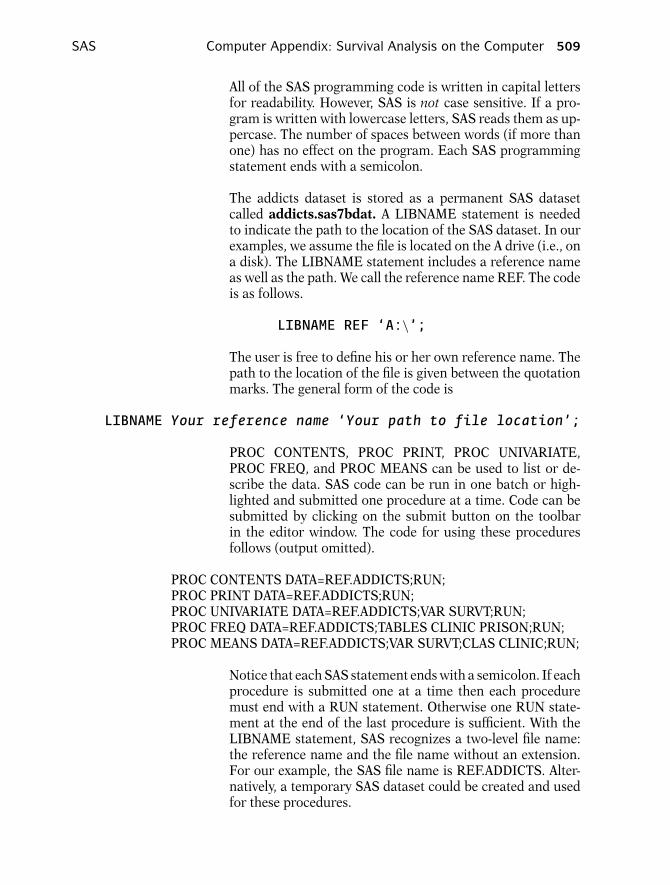
SAS Computer Appendix: Survival Analysis on the Computer 509
All of the SAS programming code is written in capital lettersfor readability. However, SAS is not case sensitive. If a pro-gram is written with lowercase letters, SAS reads them as up-percase. The number of spaces between words (if more thanone) has no effect on the program. Each SAS programmingstatement ends with a semicolon.
The addicts dataset is stored as a permanent SAS datasetcalled addicts.sas7bdat. A LIBNAME statement is neededto indicate the path to the location of the SAS dataset. In ourexamples, we assume the file is located on the A drive (i.e., ona disk). The LIBNAME statement includes a reference nameas well as the path. We call the reference name REF. The codeis as follows.
LIBNAME REF ‘A:\’;
The user is free to define his or her own reference name. Thepath to the location of the file is given between the quotationmarks. The general form of the code is
LIBNAME Your reference name ‘Your path to file location’;
PROC CONTENTS, PROC PRINT, PROC UNIVARIATE,PROC FREQ, and PROC MEANS can be used to list or de-scribe the data. SAS code can be run in one batch or high-lighted and submitted one procedure at a time. Code can besubmitted by clicking on the submit button on the toolbarin the editor window. The code for using these proceduresfollows (output omitted).
PROC CONTENTS DATA=REF.ADDICTS;RUN;PROC PRINT DATA=REF.ADDICTS;RUN;PROC UNIVARIATE DATA=REF.ADDICTS;VAR SURVT;RUN;PROC FREQ DATA=REF.ADDICTS;TABLES CLINIC PRISON;RUN;PROC MEANS DATA=REF.ADDICTS;VAR SURVT;CLAS CLINIC;RUN;
Notice that each SAS statement ends with a semicolon. If eachprocedure is submitted one at a time then each proceduremust end with a RUN statement. Otherwise one RUN state-ment at the end of the last procedure is sufficient. With theLIBNAME statement, SAS recognizes a two-level file name:the reference name and the file name without an extension.For our example, the SAS file name is REF.ADDICTS. Alter-natively, a temporary SAS dataset could be created and usedfor these procedures.

510 Computer Appendix: Survival Analysis on the Computer SAS
Text that you do not wish SAS to process should be written asa comment:
/∗ A comment begins with a forward slash followedby a star and ends with a star followed by aforward slash. ∗/
∗A comment can also be created by beginning with astar and ending with a semicolon;
The survival analyses demonstrated in SAS are:
1. Demonstrating PROC LIFETEST to obtain Kaplan–Meierand life table survival estimates (and plots);
2. Running a Cox PH model with PROC PHREG;3. Running a stratified Cox model;4. Assessing the PH assumption with a statistical test;5. Obtaining Cox adjusted survival curves;6. Running an extended Cox model (i.e., containing time-
varying covariates);7. Running parametric models with PROC LIFEREG; and8. Modeling recurrent events.
1. DEMONSTRATING PROC LIFETEST TO OBTAINKAPLAN–MEIER AND LIFE TABLE SURVIVALESTIMATES (AND PLOTS)
PROC LIFETEST produces Kaplan–Meier survival estimateswith the METHOD=KM option. The PLOTS=(S) option plotsthe estimated survival function. The TIME statement definesthe time-to-event variable (SURVT) and the value for censor-ship (STATUS = 0). The code follows (output omitted).
PROC LIFETEST DATA=REF.ADDICTS METHOD=KM PLOTS=(S);TIME SURVT∗STATUS(0);RUN;
Use a STRATA statement in PROC LIFETEST to compare sur-vival estimates for different groups (e.g., strata clinic). ThePLOTS=(S,LLS) option produces log–log curves as well as sur-vival curves. If the proportional hazard assumption is met thelog–log survival curves will be parallel. The STRATA statementalso provides the log rank test and Wilcoxon test statistics. Thecode follows.
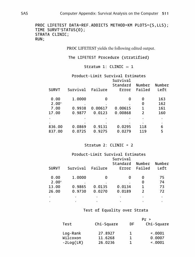
SAS Computer Appendix: Survival Analysis on the Computer 511
PROC LIFETEST DATA=REF.ADDICTS METHOD=KM PLOTS=(S,LLS);TIME SURVT∗STATUS(0);STRATA CLINIC;RUN;
PROC LIFETEST yields the following edited output.
The LIFETEST Procedure (stratified)
Stratum 1: CLINIC = 1
Product-Limit Survival EstimatesSurvivalStandard Number Number
SURVT Survival Failure Error Failed Left
0.00 1.0000 0 0 0 1632.00∗ . . . 0 1627.00 0.9938 0.00617 0.00615 1 16117.00 0.9877 0.0123 0.00868 2 160. . . . . .. . . . . .836.00 0.0869 0.9131 0.0295 118 6837.00 0.0725 0.9275 0.0279 119 5
Stratum 2: CLINIC = 2
Product-Limit Survival EstimatesSurvivalStandard Number Number
SURVT Survival Failure Error Failed Left
0.00 1.0000 0 0 0 752.00∗ . . . 0 7413.00 0.9865 0.0135 0.0134 1 7326.00 0.9730 0.0270 0.0189 2 72. . . . . .. . . . . .
Test of Equality over Strata
Pr >Test Chi-Square DF Chi-Square
Log-Rank 27.8927 1 <.0001Wilcoxon 11.6268 1 0.0007-2Log(LR) 26.0236 1 <.0001
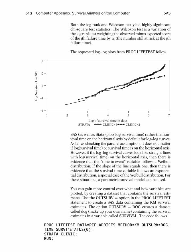
512 Computer Appendix: Survival Analysis on the Computer SAS
Both the log rank and Wilcoxon test yield highly significantchi-square test statistics. The Wilcoxon test is a variation ofthe log rank test weighting the observed minus expected scoreof the jth failure time by nj (the number still at risk at the jthfailure time).
The requested log–log plots from PROC LIFETEST follow.
2
0
−2
−4
−6
1 2 3 4 5 6 7
Log
Neg
ativ
e L
og S
DF
Log of survival time in daysCLINIC=1 CLINIC=2STRATA
SAS (as well as Stata) plots log(survival time) rather than sur-vival time on the horizontal axis by default for log–log curves.As far as checking the parallel assumption, it does not matterif log(survival time) or survival time is on the horizontal axis.However, if the log–log survival curves look like straight lineswith log(survival time) on the horizontal axis, then there isevidence that the “time-to-event” variable follows a Weibulldistribution. If the slope of the line equals one, then there isevidence that the survival time variable follows an exponen-tial distribution, a special case of the Weibull distribution. Forthese situations, a parametric survival model can be used.
You can gain more control over what and how variables areplotted, by creating a dataset that contains the survival esti-mates. Use the OUTSURV = option in the PROC LIFETESTstatement to create a SAS data containing the KM survivalestimates. The option OUTSURV = DOG creates a datasetcalled dog (make up your own name) containing the survivalestimates in a variable called SURVIVAL. The code follows.
PROC LIFETEST DATA=REF.ADDICTS METHOD=KM OUTSURV=DOG;TIME SURVT∗STATUS(0);STRATA CLINIC;RUN;

SAS Computer Appendix: Survival Analysis on the Computer 513
Data dog contains the survival estimates but not thelog(–(log)) of the survival estimates. Data cat is created inthe following code from data dog (using the statement SETDOG) and defines a new log–log variable called LLS.
DATA CAT;SET DOG;LLS=LOG(-LOG(SURVIVAL));RUN;
In SAS, the LOG function returns the natural log, not the logbase 10.
PROC PRINT prints the data in the output window.
PROC PRINT DATA=CAT; RUN;
The first 10 observations from PROC PRINT are listed below.
Obs CLINIC SURVT -CENSOR- SURVIVAL LLS
1 1 0 0 1.00000 .2 1 2 1 1.00000 .3 1 7 0 0.99383 -5.084504 1 17 0 0.98765 -4.388245 1 19 0 0.98148 -3.979656 1 28 1 0.98148 -3.979657 1 28 1 0.98148 -3.979658 1 29 0 0.97523 -3.685619 1 30 0 0.96898 -3.4573610 1 33 0 0.96273 -3.27056
The PLOT LLS∗SURVT=CLINIC statement plots the variableLLS (the log–log survival variables) on the vertical axis andSURVT on the horizontal axis, stratified by CLINIC. The SYM-BOL option can be used to choose plotting colors for eachlevel of clinic. The code and output for plotting the log–logcurves by CLINIC follow.
SYMBOL COLOR=BLUE;SYMBOL2 COLOR=RED;
PROC GPLOT DATA=CAT;PLOT LLS*SURVT=CLINIC;RUN;
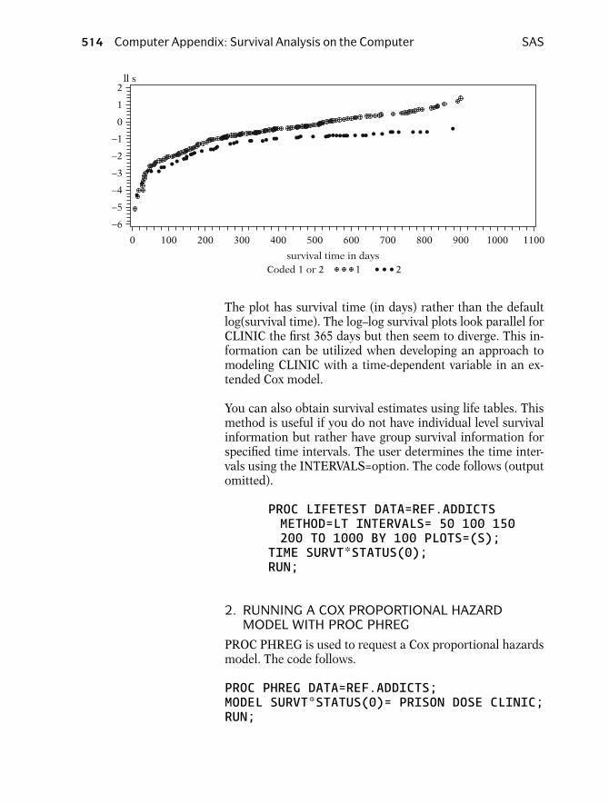
514 Computer Appendix: Survival Analysis on the Computer SAS
−6
−5
−4
−3
−2
−1
2
0
1
0 100 200 300 600500400 700 800 900 11001000
survival time in daysCoded 1 or 2 1 2
ll s
The plot has survival time (in days) rather than the defaultlog(survival time). The log–log survival plots look parallel forCLINIC the first 365 days but then seem to diverge. This in-formation can be utilized when developing an approach tomodeling CLINIC with a time-dependent variable in an ex-tended Cox model.
You can also obtain survival estimates using life tables. Thismethod is useful if you do not have individual level survivalinformation but rather have group survival information forspecified time intervals. The user determines the time inter-vals using the INTERVALS=option. The code follows (outputomitted).
PROC LIFETEST DATA=REF.ADDICTSMETHOD=LT INTERVALS= 50 100 150200 TO 1000 BY 100 PLOTS=(S);TIME SURVT*STATUS(0);RUN;
2. RUNNING A COX PROPORTIONAL HAZARDMODEL WITH PROC PHREG
PROC PHREG is used to request a Cox proportional hazardsmodel. The code follows.
PROC PHREG DATA=REF.ADDICTS;MODEL SURVT*STATUS(0)= PRISON DOSE CLINIC;RUN;
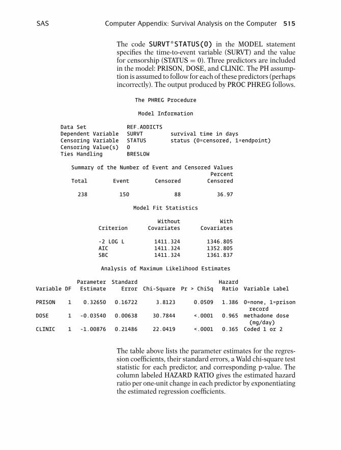
SAS Computer Appendix: Survival Analysis on the Computer 515
The code SURVT*STATUS(0) in the MODEL statementspecifies the time-to-event variable (SURVT) and the valuefor censorship (STATUS = 0). Three predictors are includedin the model: PRISON, DOSE, and CLINIC. The PH assump-tion is assumed to follow for each of these predictors (perhapsincorrectly). The output produced by PROC PHREG follows.
The PHREG Procedure
Model Information
Data Set REF.ADDICTSDependent Variable SURVT survival time in daysCensoring Variable STATUS status (0=censored, 1=endpoint)Censoring Value(s) 0Ties Handling BRESLOW
Summary of the Number of Event and Censored ValuesPercent
Total Event Censored Censored
238 150 88 36.97
Model Fit Statistics
Without WithCriterion Covariates Covariates
-2 LOG L 1411.324 1346.805AIC 1411.324 1352.805SBC 1411.324 1361.837
Analysis of Maximum Likelihood Estimates
Parameter Standard HazardVariable DF Estimate Error Chi-Square Pr > ChiSq Ratio Variable Label
PRISON 1 0.32650 0.16722 3.8123 0.0509 1.386 0=none, 1=prisonrecord
DOSE 1 -0.03540 0.00638 30.7844 <.0001 0.965 methadone dose(mg/day)
CLINIC 1 -1.00876 0.21486 22.0419 <.0001 0.365 Coded 1 or 2
The table above lists the parameter estimates for the regres-sion coefficients, their standard errors, a Wald chi-square teststatistic for each predictor, and corresponding p-value. Thecolumn labeled HAZARD RATIO gives the estimated hazardratio per one-unit change in each predictor by exponentiatingthe estimated regression coefficients.

516 Computer Appendix: Survival Analysis on the Computer SAS
You can use the TIES=EXACT option in the model statementrather than run the default TIES=BRESLOW option that wasused in the previous model. The TIES=EXACT option is acomputationally intensive method to handle events that occurat the same time. If many events occur simultaneously in thedata then the TIES=EXACT option is preferred. Otherwise,the difference between this option and the default is slight.The option RL in the MODEL statement of PROC PHREGprovides 95% confidence intervals for the hazard ratio esti-mates.
PROC PHREG DATA=REF.ADDICTS;MODEL SURVT*STATUS(0)= PRISON DOSE CLINIC/TIES=EXACT RL;RUN;
The output is shown below.
The PHREG Procedure
Model Information
Data Set REF.ADDICTSDependent Variable SURVT survival time in daysCensoring Variable STATUS status (0=censored, 1=endpoint)Censoring Value(s) 0Ties Handling EXACT
Analysis of Maximum Likelihood Estimates
Parameter Standard Hazard 95% Hazard RatioVariable DF Estimate Error Chi-Square Pr > ChiSq Ratio Confidence Limits
PRISON 1 0.32657 0.16723 3.8135 0.0508 1.386 0.999 1.924DOSE 1 -0.03537 0.00638 30.7432 <.0001 0.965 0.953 0.977CLINIC 1 -1.00980 0.21488 22.0832 <.0001 0.364 0.239 0.555
The parameter estimates and their standard errors vary onlyslightly from the previous model without the TIES=EXACToption. Notice the type of ties handling approach is listed inthe table called MODEL INFORMATION in the output.
Suppose we wish to assess interaction between PRISON andCLINIC and between PRISON and DOSE. We can define twointeraction terms in a new temporary SAS dataset (called ad-dicts2) and then run a model containing those terms. Prod-uct terms for CLINIC times PRISON (called CLIN PR) andCLINIC time DOSE (called CLIN DO) are defined in the fol-lowing data step.

SAS Computer Appendix: Survival Analysis on the Computer 517
DATA ADDICTS2;SET REF.ADDICTS;CLIN-PR=CLINIC*PRISON;CLIN-DO=CLINIC*DOSE;RUN;
The interaction terms (called CLIN PR and CLIN DO) areadded to the model.
PROC PHREG DATA=ADDICTS2;MODEL SURVT*STATUS(0)=PRISON DOSE CLINIC CLIN-PR CLIN-DO;RUN;
The PROC PHREG output follows.
The PHREG Procedure
Model Information
Data Set WORK.ADDICTS2Dependent Variable SURVT survival time in daysCensoring Variable STATUS status (0=censored, 1=endpoint)Censoring Value(s) 0Ties Handling BRESLOW
Model Fit Statistics
Without WithCriterion Covariates Covariates
-2 LOG L 1411.324 1343.199AIC 1411.324 1353.199SBC 1411.324 1368.253
Analysis of Maximum Likelihood Estimates
Parameter Standard HazardVariable DF Estimate Error Chi-Square Pr > ChiSq Ratio
PRISON 1 1.19200 0.54137 4.8480 0.0277 3.294DOSE 1 -0.01932 0.01935 0.9967 0.3181 0.981CLINIC 1 0.17469 0.89312 0.0383 0.8449 1.191CLIN-PR 1 -0.73799 0.43149 2.9253 0.0872 0.478CLIN-DO 1 -0.01386 0.01433 0.9359 0.3333 0.986
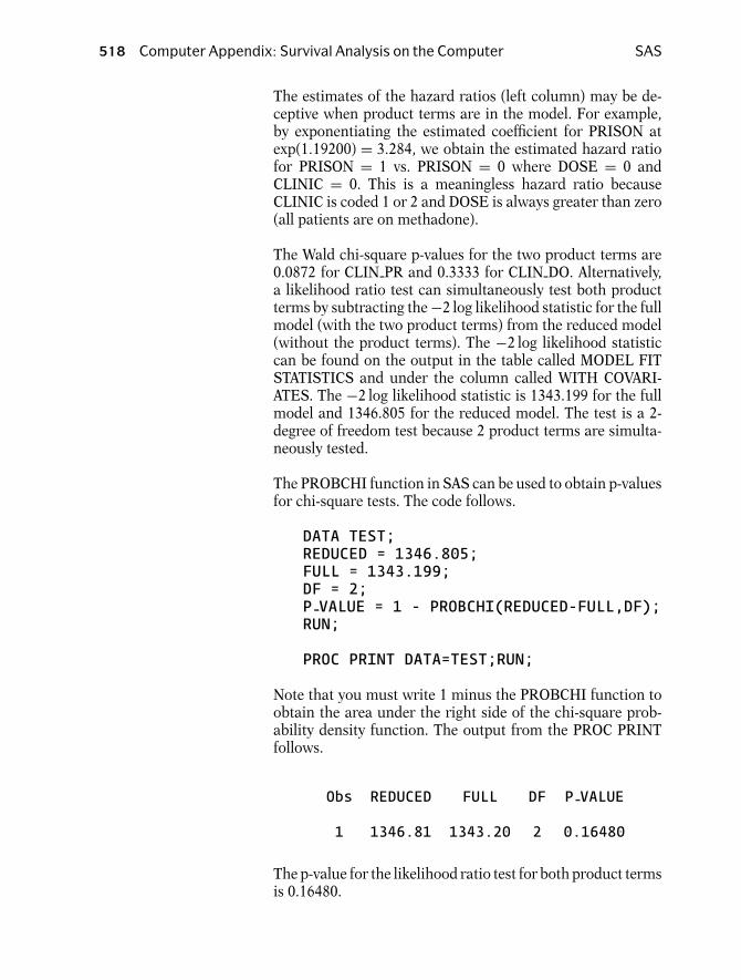
518 Computer Appendix: Survival Analysis on the Computer SAS
The estimates of the hazard ratios (left column) may be de-ceptive when product terms are in the model. For example,by exponentiating the estimated coefficient for PRISON atexp(1.19200) = 3.284, we obtain the estimated hazard ratiofor PRISON = 1 vs. PRISON = 0 where DOSE = 0 andCLINIC = 0. This is a meaningless hazard ratio becauseCLINIC is coded 1 or 2 and DOSE is always greater than zero(all patients are on methadone).
The Wald chi-square p-values for the two product terms are0.0872 for CLIN PR and 0.3333 for CLIN DO. Alternatively,a likelihood ratio test can simultaneously test both productterms by subtracting the −2 log likelihood statistic for the fullmodel (with the two product terms) from the reduced model(without the product terms). The −2 log likelihood statisticcan be found on the output in the table called MODEL FITSTATISTICS and under the column called WITH COVARI-ATES. The −2 log likelihood statistic is 1343.199 for the fullmodel and 1346.805 for the reduced model. The test is a 2-degree of freedom test because 2 product terms are simulta-neously tested.
The PROBCHI function in SAS can be used to obtain p-valuesfor chi-square tests. The code follows.
DATA TEST;REDUCED = 1346.805;FULL = 1343.199;DF = 2;P-VALUE = 1 - PROBCHI(REDUCED-FULL,DF);RUN;
PROC PRINT DATA=TEST;RUN;
Note that you must write 1 minus the PROBCHI function toobtain the area under the right side of the chi-square prob-ability density function. The output from the PROC PRINTfollows.
Obs REDUCED FULL DF P-VALUE
1 1346.81 1343.20 2 0.16480
The p-value for the likelihood ratio test for both product termsis 0.16480.

SAS Computer Appendix: Survival Analysis on the Computer 519
3. RUNNING A STRATIFIED COX MODEL
Suppose we believe that the variable CLINIC violates the pro-portional hazards assumption but the variables PRISON andDOSE follow the PH assumption within each level of CLINIC.A stratified Cox model on the variable CLINIC can be run withPROC PHREG using the STRATA CLINIC statement.
PROC PHREG DATA=REF.ADDICTS;MODEL SURVT*STATUS(0)=PRISON DOSE;STRATA CLINIC;RUN;
The output of the parameter estimates follows.
The PHREG ProcedureAnalysis of Maximum Likelihood Estimates
Parameter Standard HazardVariable DF Estimate Error Chi-Square Pr > ChiSq Ratio
PRISON 1 0.38877 0.16892 5.2974 0.0214 1.475DOSE 1 -0.03514 0.00647 29.5471 <.0001 0.965
Notice there is no parameter estimate for CLINIC be-cause CLINIC is the stratified variable. The hazard ratio forPRISON = 1 vs. PRISON = 0 is estimated at 1.475. This haz-ard ratio is assumed not to depend on CLINIC because aninteraction term between PRISON and CLINIC was not in-cluded in the model.
Suppose we wish to assess interaction between PRISON andCLINIC as well as DOSE and CLINIC in a Cox model stratifiedby CLINIC. We can define interaction terms in a new SASdataset (called addicts2) and then run a model containingthese terms. Notice that when we stratify by CLINIC we donot put the variable CLINIC in the model statement. However,the interaction terms CLIN PR and CLIN DO are put in themodel statement and CLINIC is put in the strata statement.
DATA ADDICTS2;SET REF.ADDICTS;CLIN-PR=CLINIC*PRISON;CLIN-DO=CLINIC*DOSE;RUN;
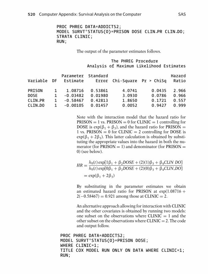
520 Computer Appendix: Survival Analysis on the Computer SAS
PROC PHREG DATA=ADDICTS2;MODEL SURVT*STATUS(0)=PRISON DOSE CLIN-PR CLIN-DO;STRATA CLINIC;RUN;
The output of the parameter estimates follows.
The PHREG ProcedureAnalysis of Maximum Likelihood Estimates
Parameter Standard HazardVariable DF Estimate Error Chi-Square Pr > ChiSq Ratio
PRISON 1 1.08716 0.53861 4.0741 0.0435 2.966DOSE 1 -0.03482 0.01980 3.0930 0.0786 0.966CLIN-PR 1 -0.58467 0.42813 1.8650 0.1721 0.557CLIN-DO 1 -0.00105 0.01457 0.0052 0.9427 0.999
Note with the interaction model that the hazard ratio forPRISON = 1 vs. PRISON = 0 for CLINIC = 1 controlling forDOSE is exp(β1 + β3), and the hazard ratio for PRISON =1 vs. PRISON = 0 for CLINIC = 2 controlling for DOSE isexp(β1 + 2β3). This latter calculation is obtained by substi-tuting the appropriate values into the hazard in both the nu-merator (for PRISON = 1) and denominator (for PRISON =0) (see below).
HR = h0(t) exp[1β1 + β2DOSE + (2)(1)β3 + β4CLIN DO]h0(t) exp[0β1 + β2DOSE + (2)(0)β3 + β4CLIN DO]
= exp(β1 + 2β3)
By substituting in the parameter estimates we obtainan estimated hazard ratio for PRISON at exp(1.08716 +2(−0.58467) = 0.921 among those at CLINIC = 2.
An alternative approach allowing for interaction with CLINICand the other covariates is obtained by running two models:one subset on the observations where CLINIC = 1 and theother subset on the observations where CLINIC = 2. The codeand output follow.
PROC PHREG DATA=ADDICTS2;MODEL SURVT*STATUS(0)=PRISON DOSE;WHERE CLINIC=1;TITLE COX MODEL RUN ONLY ON DATA WHERE CLINIC=1;RUN;
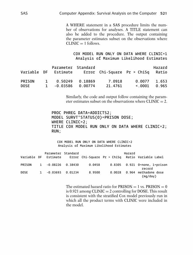
SAS Computer Appendix: Survival Analysis on the Computer 521
A WHERE statement in a SAS procedure limits the num-ber of observations for analyses. A TITLE statement canalso be added to the procedure. The output containingthe parameter estimates subset on the observations whereCLINIC = 1 follows.
COX MODEL RUN ONLY ON DATA WHERE CLINIC=1Analysis of Maximum Likelihood Estimates
Parameter Standard HazardVariable DF Estimate Error Chi-Square Pr > ChiSq Ratio
PRISON 1 0.50249 0.18869 7.0918 0.0077 1.653DOSE 1 -0.03586 0.00774 21.4761 <.0001 0.965
Similarly, the code and output follow containing the param-eter estimates subset on the observations where CLINIC = 2.
PROC PHREG DATA=ADDICTS2;MODEL SURVT*STATUS(0)=PRISON DOSE;WHERE CLINIC=2;TITLE COX MODEL RUN ONLY ON DATA WHERE CLINIC=2;RUN;
COX MODEL RUN ONLY ON DATA WHERE CLINIC=2Analysis of Maximum Likelihood Estimates
Parameter Standard HazardVariable DF Estimate Error Chi-Square Pr > ChiSq Ratio Variable Label
PRISON 1 -0.08226 0.38430 0.0458 0.8305 0.921 0=none, 1=prisonrecord
DOSE 1 -0.03693 0.01234 8.9500 0.0028 0.964 methadone dose(mg/day)
The estimated hazard ratio for PRISON = 1 vs. PRISON = 0is 0.921 among CLINIC = 2 controlling for DOSE. This resultis consistent with the stratified Cox model previously run inwhich all the product terms with CLINIC were included inthe model.

522 Computer Appendix: Survival Analysis on the Computer SAS
4. ASSESSING THE PH ASSUMPTION WITHA STATISTICAL TEST
The following SAS program makes use of the addicts datasetto demonstrate how a statistical test of the proportional haz-ard assumption is performed for a given covariate (Harrel andLee, 1986). This is accomplished by finding the correlation be-tween the Schoenfeld residuals for a particular covariate andthe ranking of individual failure times. If the proportionalhazard assumption is met then the correlation should be nearzero.
The p-value for testing this correlation can be obtained fromPROC CORR (or PROC REG). The Schoenfeld residuals fora given model can be saved in a SAS dataset using PROCPHREG. The ranking of events by failure time can be savedin a SAS dataset using PROC RANKED. The null hypothesisis that the PH assumption is not violated.
First run the full model. The output statement creates aSAS dataset, the OUT=option defines an output dataset, andthe RESSCH=statement is followed by user-defined variablenames so that the output dataset contains the Schoenfeldresiduals. The order of the names corresponds to the orderof the independent variables in the model statement. The ac-tual variable names are arbitrary. The name we chose for thedataset is RESID and the names we chose for the variablescontaining the Schoenfeld residuals for CLINIC, PRISON,and DOSE are RCLINIC, RPRISON, and RDOSE. The codefollows.
PROC PHREG DATA=REF.ADDICTS;MODEL SURVT*STATUS(0)=CLINIC PRISON DOSE;OUTPUT OUT=RESID RESSCH=RCLINIC RPRISON RDOSE;RUN;
PROC PRINT DATA=RESID;RUN;

SAS Computer Appendix: Survival Analysis on the Computer 523
The first 10 observations of the PROC PRINT are shown be-low. The three columns on the right are the variables contain-ing the Schoenfeld residuals.
Obs SURVT STATUS CLINIC PRISON DOSE RCLINIC RPRISON RDOSE
1 428 1 1 0 50 -0.18715 -0.40641 -8.21002 275 1 1 1 55 -0.15841 0.55485 -2.62773 262 1 1 0 55 -0.16453 -0.45197 -2.56354 183 1 1 0 30 -0.14577 -0.48727 -26.08235 259 1 1 1 65 -0.16306 0.54313 7.37016 714 1 1 0 55 -0.25853 -0.50074 -8.53477 438 1 1 1 65 -0.19292 0.58106 6.60728 796 0 1 1 60 . . .9 892 1 1 0 50 -0.34478 -0.22372 -15.908810 393 1 1 1 65 -0.17712 0.57376 6.6886
Next, create a SAS dataset that deletes censored observations(i.e., only contains observations that fail).
DATA EVENTS;SET RESID;IF STATUS=1;RUN;
Use PROC RANK to create a dataset containing a variablethat ranks the order of failure times. The user supplies thename of the output data set using the OUT= option. The vari-able to be ranked is SURVT (the survival time variable). TheRANKS statement precedes a user-defined variable name forthe rankings of failure times. The user-defined names are ar-bitrary. The name we chose for this variable is TIMERANK.The code follows.
PROC RANK DATA=EVENTS OUT=RANKED TIES=MEAN;VAR SURVT;RANKS TIMERANK;RUN;
PROC PRINT DATA=RANKED;RUN;
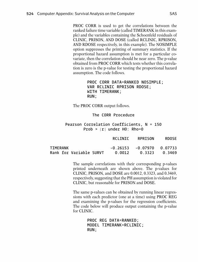
524 Computer Appendix: Survival Analysis on the Computer SAS
PROC CORR is used to get the correlations between theranked failure time variable (called TIMERANK in this exam-ple) and the variables containing the Schoenfeld residuals ofCLINIC, PRISON, AND DOSE (called RCLINIC, RPRISON,AND RDOSE respectively, in this example). The NOSIMPLEoption suppresses the printing of summary statistics. If theproportional hazard assumption is met for a particular co-variate, then the correlation should be near zero. The p-valueobtained from PROC CORR which tests whether this correla-tion is zero is the p-value for testing the proportional hazardassumption. The code follows.
PROC CORR DATA=RANKED NOSIMPLE;VAR RCLINIC RPRISON RDOSE;WITH TIMERANK;RUN;
The PROC CORR output follows.
The CORR Procedure
Pearson Correlation Coefficients, N = 150Prob > |r | under H0: Rho=0
RCLINIC RPRISON RDOSE
TIMERANK -0.26153 -0.07970 0.07733Rank for Variable SURVT 0.0012 0.3323 0.3469
The sample correlations with their corresponding p-valuesprinted underneath are shown above. The p-values forCLINIC, PRISON, and DOSE are 0.0012, 0.3323, and 0.3469,respectively, suggesting that the PH assumption is violated forCLINIC, but reasonable for PRISON and DOSE.
The same p-values can be obtained by running linear regres-sions with each predictor (one at a time) using PROC REGand examining the p-values for the regression coefficients.The code below will produce output containing the p-valuefor CLINIC.
PROC REG DATA=RANKED;MODEL TIMERANK=RCLINIC;RUN;

SAS Computer Appendix: Survival Analysis on the Computer 525
The output produced by PROC REG follows.
The REG Procedure
Parameter Estimates
Parameter StandardVariable Estimate Error t Value Pr > |t |
Intercept 75.49955 3.43535 21.98 <.0001RCLINIC -28.38848 8.61194 -3.30 0.0012
The p-value for CLINIC (0.0012) is shown in the column onthe right and matches the p-value that was obtained usingPROC CORR.
5. OBTAINING COX ADJUSTED SURVIVAL CURVES
We can use the BASELINE statement in PROC PHREG tocreate an output dataset containing Cox adjusted survival es-timates for a specified pattern of covariates. The particularpattern of covariates of interest must first be created in a SASdataset that is subsequently used as the input dataset for theCOVARIATES=option in the BASELINE statement of PROCPHREG. Each pattern of covariates yields a different sur-vival curve (assuming nonzero effects). Adjusted log(− log)survival plots can also be obtained for assessing the PH as-sumption. This is illustrated with three examples.
Ex1—Run a PH model using PRISON, DOSE, and CLINIC andobtain adjusted survival curves where PRISON = 0, DOSE =70, and CLINIC = 2.
Ex2—Run a stratified Cox model (by CLINIC). Obtain two ad-justed survival curves using the mean value of PRISON andDOSE for CLINIC = 1 and CLINIC = 2. Use the log–log curvesto assess the PH assumption for CLINIC adjusted for PRISONand DOSE.
Ex3—Run a stratified Cox model (by CLINIC) and obtain ad-justed survival curves for PRISON = 0, DOSE = 70, and forPRISON = 1, DOSE = 70. This yields four survival curves inall, two for CLINIC = 1 and two for CLINIC = 2.

526 Computer Appendix: Survival Analysis on the Computer SAS
Basically there are these steps:
1. Create the input dataset containing the pattern (values) ofcovariates used for the adjusted survival curves.
2. Run a Cox model with PROC PHREG using the BASELINEstatement to input the dataset from Step (1) and output adataset containing the adjusted survival estimates.
3. Plot the adjusted survival estimates from the output datasetcreated in Step (2).
For Ex1 we create an input dataset (called IN1) with one ob-servation where PRISON = 0, DOSE = 70, and CLINIC =2. We then run a model and create an output dataset (calledOUT1) containing a variable with the adjusted survival esti-mates (called S1). Finally, the adjusted survival curve is plot-ted using PROC GPLOT. The code follows.
DATA IN1;INPUT PRISON DOSE CLINIC;CARDS;0 70 2;
PROC PHREG DATA=REF.ADDICTS;MODEL SURVT*STATUS(0)=PRISON DOSE CLINIC;BASELINE COVARIATES=IN1 OUT=OUT1 SURVIVAL=S1/NOMEAN;RUN;
PROC GPLOT DATA=OUT1;PLOT S1*SURVT;TITLE Adjusted survival for prison=0, dose=70, clinic=2;RUN;
The BASELINE statement in PROC PHREG specifies the in-put dataset, the output dataset, and the name of the variablecontaining the adjusted survival estimates. The NOMEAN op-tion suppresses the survival estimates using the mean valuesof PRISON, DOSE, and CLINIC. The next example (Ex2) doesnot use the NOMEAN option.
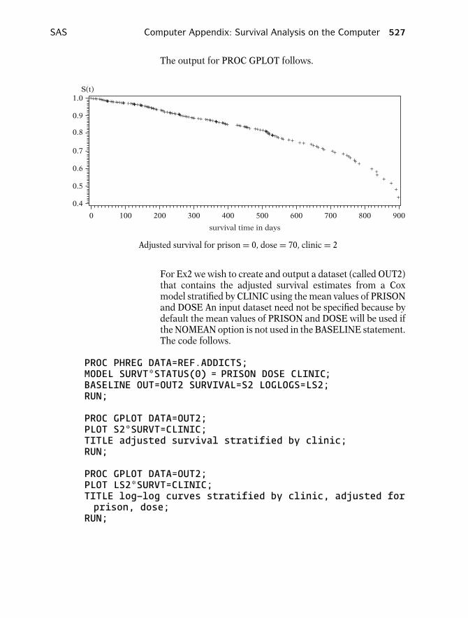
SAS Computer Appendix: Survival Analysis on the Computer 527
The output for PROC GPLOT follows.
1000 200 300 400 500 600 700 800 900
survival time in days
1.0
0.9
0.8
0.7
0.6
0.5
0.4
S(t)
Adjusted survival for prison = 0, dose = 70, clinic = 2
For Ex2 we wish to create and output a dataset (called OUT2)that contains the adjusted survival estimates from a Coxmodel stratified by CLINIC using the mean values of PRISONand DOSE An input dataset need not be specified because bydefault the mean values of PRISON and DOSE will be used ifthe NOMEAN option is not used in the BASELINE statement.The code follows.
PROC PHREG DATA=REF.ADDICTS;MODEL SURVT*STATUS(0) = PRISON DOSE CLINIC;BASELINE OUT=OUT2 SURVIVAL=S2 LOGLOGS=LS2;RUN;
PROC GPLOT DATA=OUT2;PLOT S2*SURVT=CLINIC;TITLE adjusted survival stratified by clinic;RUN;
PROC GPLOT DATA=OUT2;PLOT LS2*SURVT=CLINIC;TITLE log–log curves stratified by clinic, adjusted forprison, dose;RUN;

528 Computer Appendix: Survival Analysis on the Computer SAS
The code PLOT LS2∗SURVT=CLINIC in the second PROCGPLOT will plot LS2 on the vertical axis, SURVT on the hori-zontal axis, stratified by CLINIC on the same graph. The vari-able LS2 was created in the BASELINE statement of PROCPHREG and contains the adjusted log–log survival estimates.The PROC GPLOT output for the log–log survival curves strat-ified by CLINIC adjusted for PRISON and DOSE follows.
−6
−5
−4
−3
−2
−1
2
0
1
0 100 200 300 600500
survival time in days
400 700 800 900
Coded 1 or 2 1 2
Log
of
Neg
ativ
e L
og o
f S
UR
VIV
AL
Log–log curves stratified by clinic, adjusted for prison, dose
The adjusted log–log plots look similar to the unadjusted log–log Kaplan–Meier plots shown earlier in that the plots lookreasonably parallel before 365 days but then diverge suggest-ing that the PH assumption is violated after 1 year.
For Ex3, a stratified Cox (by CLINIC) is run and adjustedcurves are obtained for PRISON = 1 and PRISON = 0 holdingDOSE = 70. An input dataset (called IN3) is created with twoobservations for both levels of PRISON with DOSE = 70. Anoutput dataset (called OUT3) is created with the BASELINEstatement that contains a variable (called S3) of survival es-timates for all four curves (two for each stratum of CLINIC).The code follows.

SAS Computer Appendix: Survival Analysis on the Computer 529
DATA IN3;INPUT PRISON DOSE;CARDS;1 700 70;
PROC PHREG DATA=REF.ADDICTS;MODEL SURVT*STATUS(0)= PRISON DOSE;STRATA CLINIC;BASELINE COVARIATES=IN3 OUT=OUT4 SURVIVAL=S3/NOMEAN;RUN;
PROC GPLOT DATA=OUT3;PLOT S3*SURVT=CLINIC;TITLE adjusted survival stratified by clinic for both levelsof prison;RUN;
The PROC GPLOT output follows.
0 100 200 300 400 500 600 700 800 900
survival time in daysCoded 1 or 2 1 2
0.0
0.1
0.2
0.3
0.4
0.5
0.6
0.7
0.8
1.0
0.9
Su
rviv
al f
un
ctio
n e
stim
ate
Adjusted survival stratified by clinic for both levels of prison
For the above graph, the PH assumption is not assumed forCLINIC because that is the stratified variable. However, thePH assumption is assumed for PRISON within each stratumof CLINIC (i.e., CLINIC = 1 and CLINIC = 2).
530 Computer Appendix: Survival Analysis on the Computer SAS
6. RUNNING AN EXTENDED COX MODEL
Models containing time-dependent variables are run usingPROC PHREG. Time-dependent variables are created withprogramming statements within the PROC PHREG proce-dure. Sometimes users incorrectly define time-dependentvariables in the data step. This leads to wrong estimates be-cause the time variable used in the data step (SURVT) is ac-tually time-independent and therefore different than the timevariable (also called SURVT) used to define time-dependentvariables in the PROC PHREG statement. See the discussionon the extended Cox likelihood in Chapter 6 for further clari-fication of this issue.
We have evaluated the PH assumption for the variable CLINICby plotting KM log–log curves and Cox adjusted log–log curvesstratified by CLINIC and checking whether the curves wereparallel. We could do similar analyses with the variablesPRISON and DOSE although with DOSE we would need tocategorize the continuous variable before comparing plots fordifferent strata of DOSE.
If it is expected that the hazard ratio for the effect of DOSEincreases (or decreases) monotonically with time we couldadd a continuous time-varying product term with DOSE andsome function of time. The model defined below contains atime-varying variable (LOGTDOSE) defined as the product ofDOSE and the natural log of time (SURVT). In some sense aviolation of the proportional hazard assumption for a partic-ular variable means that there is an interaction between thatvariable and time. Note that the variable LOGTDOSE is de-fined within the PHREG procedure and not in the data step.The code follows.
PROC PHREG DATA=REF.ADDICTS;MODEL SURVT*STATUS(0)=PRISON CLINIC DOSE LOGTDOSE;LOGTDOSE=DOSE*LOG(SURVT);RUN;

SAS Computer Appendix: Survival Analysis on the Computer 531
The output produced by PROC PHREG follows.
The PHREG ProcedureAnalysis of Maximum Likelihood Estimates
Parameter Standard HazardVariable DF Estimate Error Chi-Square Pr > ChiSq Ratio
PRISON 1 0.34047 0.16747 4.1333 0.0420 1.406CLINIC 1 -1.01857 0.21538 22.3655 <.0001 0.361DOSE 1 -0.08243 0.03599 5.2468 0.0220 0.921LOGTDOSE 1 0.00858 0.00646 1.7646 0.1841 1.009
The Wald test for the time-dependent variable LOGTDOSEyields a p-value of 0.1841. A nonsignificant p-value does notnecessarily mean that the PH assumption is reasonable forDOSE. Perhaps a different defined time-dependent variablewould have been significant (e.g., DOSE × (TIME − 100)).Also the sample size of the study is a key determinant of thepower to reject the null, which in this case means rejection ofthe PH assumption.
Next we consider time-dependent variables for CLINIC. Thenext two models use Heaviside functions that allow a differenthazard ratio for CLINIC before and after 365 days. The firstmodel uses two Heaviside functions in the model (HV1 andHV2) but not CLINIC. The second model uses one Heavisidefunction (HV) but also includes CLINIC in the model. Thesetwo models yield the same hazard ratio estimates for CLINICbut are coded differently. The code follows.
PROC PHREG DATA=REF.ADDICTS;MODEL SURVT*STATUS(0)=PRISON DOSE HV1 HV2;IF SURVT < 365 THEN HV1 = CLINIC; ELSE HV1 = 0;IF SURVT >= 365 THEN HV2 = CLINIC; ELSE HV2 = 0;RUN;
PROC PHREG DATA=REF.ADDICTS;MODEL SURVT*STATUS(0)=CLINIC PRISON DOSE HV;IF SURVT >= 365 THEN HV = CLINIC; ELSE HV = 0;RUN;

532 Computer Appendix: Survival Analysis on the Computer SAS
The output for the model with two Heaviside functionsfollows.
The PHREG ProcedureAnalysis of Maximum Likelihood Estimates
Parameter Standard HazardVariable DF Estimate Error Chi-Square Pr > ChiSq Ratio
PRISON 1 0.37770 0.16840 5.0304 0.0249 1.459DOSE 1 -0.03551 0.00644 30.4503 <.0001 0.965HV1 1 -0.45956 0.25529 3.2405 0.0718 0.632HV2 1 -1.82823 0.38595 22.4392 <.0001 0.161
The parameter estimates for HV1 and HV2 can be used di-rectly to obtain the estimated hazard ratio for CLINIC = 2vs. CLINIC = 1 before and after 365 days. The estimated haz-ard ratio for CLINIC at 100 days is exp(−0.45956) = 0.632and the estimated hazard ratio for CLINIC at 400 days isexp(−1.82823) = 0.161.
The output for the model with one Heaviside function follows.
The PHREG ProcedureAnalysis of Maximum Likelihood Estimates
Parameter Standard HazardVariable DF Estimate Error Chi-Square Pr > ChiSq Ratio
CLINIC 1 -0.45956 0.25529 3.2405 0.0718 0.632PRISON 1 0.37770 0.16840 5.0304 0.0249 1.459DOSE 1 -0.03551 0.00644 30.4503 <.0001 0.965HV 1 -1.36866 0.46139 8.7993 0.0030 0.254
Notice the variable CLINIC is included in this model andthe coefficient for the time-dependent Heaviside functionHV does not contribute to the estimated hazard ratio un-til day 365. The estimated hazard ratio for CLINIC at 100days is exp(−0.45956) = 0.632 and the estimated hazard ratiofor CLINIC at 400 days is exp((−0.45956) + (−1.36866)) =0.161. These results are consistent with the estimates ob-tained from the model with two Heaviside functions. A Waldtest for the variable HV shows a statistically significant p-value of 0.003 suggesting a violation of the PH assumptionfor CLINIC.
SAS Computer Appendix: Survival Analysis on the Computer 533
Suppose it is believed that the hazard ratio for CLINIC = 2 vs.CLINIC = 1 is constant over the first year but then monoton-ically increases (or decreases) after the first year. The follow-ing code defines a model allowing for a time-varying covariatecalled CLINTIME (defined in the code) which contributes tothe hazard ratio for CLINIC after 365 days. The code follows(output omitted).
PROC PHREG DATA=REF.ADDICTS;MODEL SURVT*STATUS(0)=CLINIC PRISON DOSE CLINTIME;IF SURVT < 365 THEN CLINTIME=0;ELSE IF SURVT >= 365 THEN CLINTIME = CLINIC*(SURVT-365);RUN;
7. RUNNING PARAMETRIC MODELSWITH PROC LIFEREG
PROC LIFEREG runs parametric accelerated failure time(AFT) models rather than proportional hazards (PH) mod-els. Whereas the key assumption of a PH model is that haz-ard ratios are constant over time, the key assumption for anAFT model is that survival time accelerates (or decelerates)by a constant factor when comparing different levels ofcovariates.
The most common distribution for parametric modeling ofsurvival data is the Weibull distribution. The hazard functionfor a Weibull distribution is λptp−1. If p = 1 then the Weibulldistribution is also an exponential distribution. The Weibulldistribution has a desirable property in that if the AFT as-sumption holds then the PH assumption also holds. The ex-ponential distribution is a special case of the Weibull distri-bution. The key property for the exponential distribution isthat the hazard is constant over time (h(t) = λ). In SAS, theWeibull and exponential model are run only as AFT models.
The Weibull distribution has the property that the log–logof the survival function is linear with the log of time. PROCLIFETEST can be used to plot Kaplan–Meier log–log curvesagainst the log of time. If the curves are approximatelystraight lines (and parallel) then the assumption is reason-able. Furthermore, if the straight lines have a slope of 1, thenthe exponential distribution is appropriate. The code belowproduces log–log curves stratified by CLINIC and PRISONthat can be used to check the validity of the Weibull assump-tion for those variables.
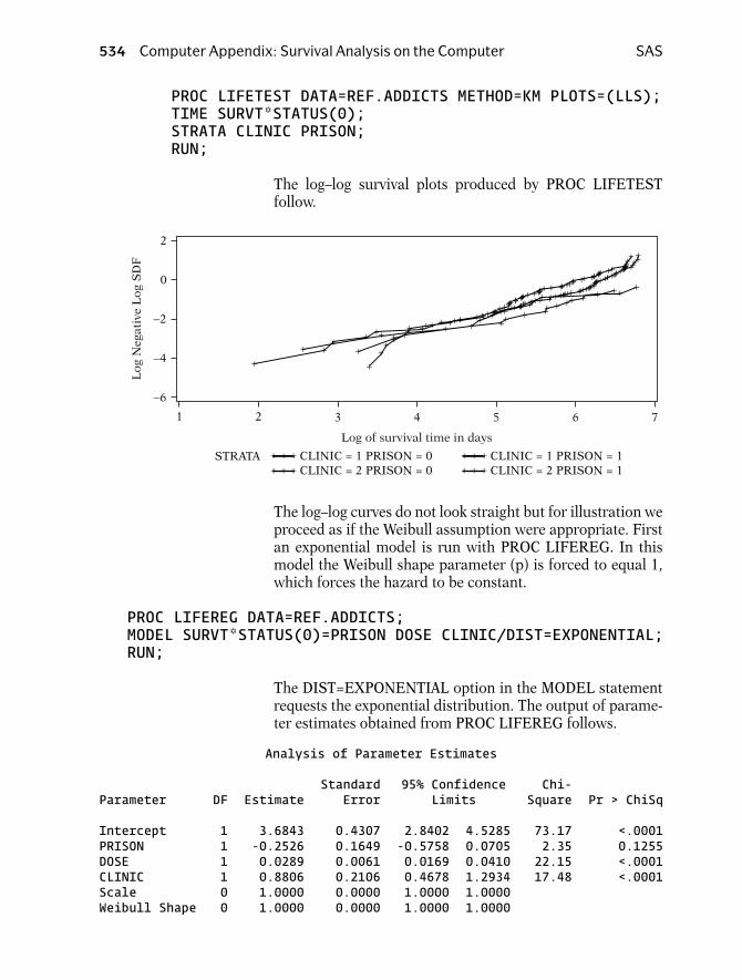
534 Computer Appendix: Survival Analysis on the Computer SAS
PROC LIFETEST DATA=REF.ADDICTS METHOD=KM PLOTS=(LLS);TIME SURVT*STATUS(0);STRATA CLINIC PRISON;RUN;
The log–log survival plots produced by PROC LIFETESTfollow.
2
0
−2
−4
−6
Log
Neg
ativ
e L
og S
DF
321 4 5 6 7
Log of survival time in days
CLINIC = 2 PRISON = 0CLINIC = 1 PRISON = 1CLINIC = 2 PRISON = 1
CLINIC = 1 PRISON = 0STRATA
The log–log curves do not look straight but for illustration weproceed as if the Weibull assumption were appropriate. Firstan exponential model is run with PROC LIFEREG. In thismodel the Weibull shape parameter (p) is forced to equal 1,which forces the hazard to be constant.
PROC LIFEREG DATA=REF.ADDICTS;MODEL SURVT*STATUS(0)=PRISON DOSE CLINIC/DIST=EXPONENTIAL;RUN;
The DIST=EXPONENTIAL option in the MODEL statementrequests the exponential distribution. The output of parame-ter estimates obtained from PROC LIFEREG follows.
Analysis of Parameter Estimates
Standard 95% Confidence Chi-Parameter DF Estimate Error Limits Square Pr > ChiSq
Intercept 1 3.6843 0.4307 2.8402 4.5285 73.17 <.0001PRISON 1 -0.2526 0.1649 -0.5758 0.0705 2.35 0.1255DOSE 1 0.0289 0.0061 0.0169 0.0410 22.15 <.0001CLINIC 1 0.8806 0.2106 0.4678 1.2934 17.48 <.0001Scale 0 1.0000 0.0000 1.0000 1.0000Weibull Shape 0 1.0000 0.0000 1.0000 1.0000

SAS Computer Appendix: Survival Analysis on the Computer 535
The exponential model assumes a constant hazard. This is in-dicated in the output by the value of the Weibull shape pa-rameter (1.0000). The output can be used to calculate theestimated hazard for any subject given a pattern of covari-ates. For example, a subject with PRISON = 0, DOSE = 50,and CLINIC = 2 has an estimated hazard of exp(−(3.6843 +50(0.0289) + 2(0.8806)) = .001. Note that SAS gives the pa-rameter estimates for the AFT form of the exponential model.Multiply the estimated coefficients by negative one to get esti-mates consistent with the PH parameterization of the model(see Chapter 7).
Next a Weibull AFT model is run with PROC LIFEREG.
PROC LIFEREG DATA=REF.ADDICTS;MODEL SURVT*STATUS(0)=PRISON DOSE CLINIC/DIST=WEIBULL;RUN;
The DIST=WEIBULL option in the MODEL statement re-quests the Weibull distribution. The output for the parameterestimates follows.
Analysis of Parameter Estimates
Standard 95% Confidence Chi-Parameter DF Estimate Error Limits Square Pr > ChiSq
Intercept 1 4.1048 0.3281 3.4619 4.7478 156.56 <.0001PRISON 1 -0.2295 0.1208 -0.4662 0.0073 3.61 0.0575DOSE 1 0.0244 0.0046 0.0154 0.0334 28.32 <.0001CLINIC 1 0.7090 0.1572 0.4009 1.0172 20.34 <.0001Scale 1 0.7298 0.0493 0.6393 0.8332Weibull Shape 1 1.3702 0.0926 1.2003 1.5642
The Weibull shape parameter is estimated at 1.3702. SAS callsthe reciprocal of the Weibull shape parameter, the Scale pa-rameter, estimated at 0.7298. The acceleration factor compar-ing CLINIC = 2 to CLINIC = 1 is estimated at exp(0.7090) =2.03. So the estimated median survival time (time off heroin)is double for patients enrolled in CLINIC = 2 compared toCLINIC = 1.
To obtain the hazard ratio parameters from the Weibull AFTmodel, multiply the Weibull shape parameter by the negativeof the AFT parameter (see Chapter 7). For example, the HRestimate for CLINIC = 2 vs. CLINIC = 1 controlling for theother covariates is exp(1.3702(−0.7090)) = 0.38.
536 Computer Appendix: Survival Analysis on the Computer SAS
Next a log-logistic AFT model is run with PROC LIFEREG.
PROC LIFEREG DATA=REF.ADDICTS;MODEL SURVT*STATUS(0)=PRISON DOSE CLINIC/DIST=LLOGISTIC;RUN;
The output of the log-logistic parameter estimates follows.
Analysis of Parameter Estimates
Standard 95% Confidence Chi-Parameter DF Estimate Error Limits Square Pr >ChiSq
Intercept 1 3.5633 0.3894 2.8000 4.3266 83.71 <.0001PRISON 1 -0.2913 0.1440 -0.5734 -0.0091 4.09 0.0431DOSE 1 0.0316 0.0055 0.0208 0.0424 32.81 <.0001CLINIC 1 0.5806 0.1716 0.2443 0.9169 11.45 0.0007Scale 1 0.5868 0.0403 0.5129 0.6712
From this output, the acceleration factor comparingCLINIC = 2 to CLINIC = 1 is estimated as exp(0.5806) =1.79. If the AFT assumption holds for a log-logistic model,then the proportional odds assumption holds for the survivalfunction (although the PH assumption will not hold). The pro-portional odds assumption can be evaluated by plotting thelog odds of survival (using KM estimates) against the log ofsurvival time. If the plots are straight lines for each pattern ofcovariates then the log-logistic distribution is reasonable. Ifthe straight lines are also parallel then the proportional oddsand AFT assumptions also hold.
A SAS dataset containing the KM survival estimates can becreated using PROC LIFETEST (see Section 1 of this ap-pendix). Once this variable is created, a dataset containingvariables for the estimated log odds of survival and the log ofsurvival time can also be created. PROC GPLOT can then beused to plot the log odds of survival against survival time.
Another context for thinking about the proportional odds as-sumption is that the odds ratio estimated by a logistic re-gression does not depend on the length of the follow-up. Forexample, if a follow-up study were extended from three to fiveyears then the underlying odds ratio comparing two patternsof covariates would not change. If the proportional odds as-sumption is not true, then the odds ratio is specific to thelength of follow-up.

SAS Computer Appendix: Survival Analysis on the Computer 537
An AFT model is a multiplicative model with respect to sur-vival time or equivalently an additive model with respect to thelog of time. In the previous example, the median survival timewas estimated as 1.79 times longer for CLINIC = 2 comparedto CLINIC = 1. In that example survival time was assumedto follow a log-logistic distribution or equivalently the log ofsurvival time was assumed to follow a logistic distribution.
SAS allows additive failure time models to be run (seeChapter 7 under the heading “Other Parametric Models”). TheNOLOG option in the MODEL statement of PROC LIFEREGsuppresses the default log link function which means thattime, rather than log(time), is modeled as a linear functionof the regression parameters. The following code requests anadditive failure time model in which time follows a logistic(not log-logistic) distribution.
PROC LIFEREG DATA=REF.ADDICTS;MODEL SURVT*STATUS(0)=PRISON DOSE CLINIC/DIST=LLOGISTIC NOLOG;RUN;
Even though the option DIST=LLOGISTIC appears to re-quest that survival time follow a log-logistic distribution, theNOLOG option actually means that survival time is assumedto follow a logistic distribution. (Note that the NOLOG op-tion in Stata means something completely different using thestreg command: that the iteration log file not be shown inthe output.) The output from the additive failure time modelfollows.
Analysis of Parameter Estimates
Standard 95% Confidence Chi-Parameter DF Estimate Error Limits Square Pr > ChiSq
Intercept 1 -358.482 114.0161 -581.949 -135.014 9.89 0.0017PRISON 1 -89.7816 42.9645 -173.990 -5.5727 4.37 0.0366DOSE 1 10.3893 1.6244 7.2055 13.5731 40.91 <.0001CLINIC 1 214.2525 53.1204 110.1385 318.3665 16.27 <.0001Scale 1 172.4039 11.3817 151.4792 196.2191
538 Computer Appendix: Survival Analysis on the Computer SAS
The parameter estimate for CLINIC is 214.2525. The inter-pretation for this estimate is that the median survival time(or time to any fixed value of S(t)) is estimated at 214 daysmore for CLINIC = 2 compared to CLINIC = 1. In otherwords, you add 214 days to the estimated median survivaltime for CLINIC = 1 to get the estimated median survivaltime for CLINIC = 2. This contrasts with the previous AFTmodel in which you multiply estimated median survival timefor CLINIC = 1 by 1.79 to get the estimated median survivaltime for CLINIC = 2. The additive model can be viewed as ashifting of survival time whereas the AFT model can be viewedas a scaling of survival time.
If survival time follows a logistic distribution and the ad-ditive failure time assumption holds, then the proportionalodds assumption also holds. The logistic assumption can beevaluated by plotting the log odds of survival (using KM es-timates) against time (rather than against the log of time asanalogously used for the evaluation of the log-logistic assump-tion). If the plots are straight lines for each pattern of covari-ates then the logistic distribution is reasonable. If the straightlines are also parallel then the proportional odds and additivefailure time assumptions hold.
Other distributions supported by PROC LIFEREG arethe generalized gamma (DIST=GAMMA) and lognormal(DIST=LNORMAL) distributions. If the NOLOG option isspecified with the DIST=LNORMAL option in the model state-ment, then survival time is assumed to follow a normal dis-tribution. SAS version 8.2 does not support frailty survivalmodels.
8. MODELING RECURRENT EVENTS
The modeling of recurrent events is illustrated with the blad-der cancer dataset (bladder.sas7bdat) described at the startof this appendix. Recurrent events are represented in thedata with multiple observations for subjects having multipleevents. The data layout for the bladder cancer dataset is suit-able for a counting process approach with time intervals de-fined for each observation (see Chapter 8). The following codeprints the 12th through 20th observation, which contains in-formation for four subjects. The code follows.
PROC PRINT DATA=REF.BLADDER (FIRSTOBS= 12 OBS=20);RUN;
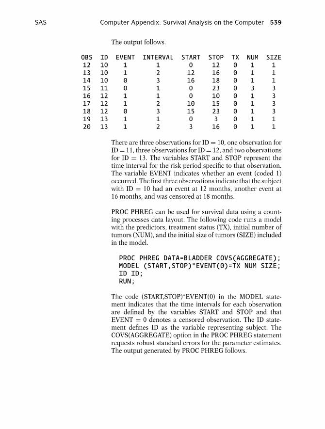
SAS Computer Appendix: Survival Analysis on the Computer 539
The output follows.
OBS ID EVENT INTERVAL START STOP TX NUM SIZE12 10 1 1 0 12 0 1 113 10 1 2 12 16 0 1 114 10 0 3 16 18 0 1 115 11 0 1 0 23 0 3 316 12 1 1 0 10 0 1 317 12 1 2 10 15 0 1 318 12 0 3 15 23 0 1 319 13 1 1 0 3 0 1 120 13 1 2 3 16 0 1 1
There are three observations for ID = 10, one observation forID = 11, three observations for ID = 12, and two observationsfor ID = 13. The variables START and STOP represent thetime interval for the risk period specific to that observation.The variable EVENT indicates whether an event (coded 1)occurred. The first three observations indicate that the subjectwith ID = 10 had an event at 12 months, another event at16 months, and was censored at 18 months.
PROC PHREG can be used for survival data using a count-ing processes data layout. The following code runs a modelwith the predictors, treatment status (TX), initial number oftumors (NUM), and the initial size of tumors (SIZE) includedin the model.
PROC PHREG DATA=BLADDER COVS(AGGREGATE);MODEL (START,STOP)*EVENT(0)=TX NUM SIZE;ID ID;RUN;
The code (START,STOP)∗EVENT(0) in the MODEL state-ment indicates that the time intervals for each observationare defined by the variables START and STOP and thatEVENT = 0 denotes a censored observation. The ID state-ment defines ID as the variable representing subject. TheCOVS(AGGREGATE) option in the PROC PHREG statementrequests robust standard errors for the parameter estimates.The output generated by PROC PHREG follows.

540 Computer Appendix: Survival Analysis on the Computer SAS
The PHREG Procedure
Model Information
Data Set WORK.BLADDERDependent Variable STARTDependent Variable STOPCensoring Variable EVENTCensoring Value(s) 0Ties Handling BRESLOW
Analysis of Maximum Likelihood Estimates
Parameter Standard StdErr HazardVariable Estimate Error Ratio Chi-Square Pr > ChiSq Ratio
TX -0.40710 0.24183 1.209 2.8338 0.0923 0.666NUM 0.16065 0.05689 1.185 7.9735 0.0047 1.174SIZE -0.04009 0.07222 1.028 0.3081 0.5788 0.961
Coefficient estimates are provided with robust standard er-rors. The column under the heading StdErrRatio providesthe ratio of the robust to the nonrobust standard errors.For example, the standard error for the coefficient for TX(0.24183) is 1.209 greater than the standard error would beif we had not requested robust standard errors (i.e., omit theCOVS(AGGREGATE) option). The robust standard errors areestimated slightly differently compared to the correspondingmodel in Stata.
A stratified Cox model can also be run using the data in thisformat with the variable INTERVAL as the stratified variable.The stratified variable indicates whether the subject was atrisk for a 1st, 2nd, 3rd, or 4th event. This approach is calledconditional 1 in Chapter 8 and is used if the investigatorwants to distinguish the order in which recurrent events oc-cur. The code for a stratified Cox follows.
PROC PHREG DATA=BLADDER COVS(AGGREGATE);MODEL (START,STOP)*EVENT(0)=TX NUM SIZE;ID ID;STRATA INTERVAL;RUN;

SAS Computer Appendix: Survival Analysis on the Computer 541
The only additional code from the previous model is theSTRATA statement indicating that the variable INTERVAL isthe stratified variable. The output containing the parameterestimates follows.
Analysis of Maximum Likelihood Estimates
Parameter Standard StdErr HazardVariable Estimate Error Ratio Chi-Square Pr > ChiSq Ratio
TX -0.33430 0.19706 0.912 2.8777 0.0898 0.716NUM 0.11565 0.04991 0.930 5.3690 0.0205 1.123SIZE -0.00805 0.06012 0.827 0.0179 0.8935 0.992
Interaction terms between the treatment variable (TX) andthe stratified variable could be created to examine whetherthe effect of treatment differed for the 1st, 2nd, 3rd, or 4thevent.
Another stratified approach (called conditional 2) is a slightvariation of the conditional 1 approach. The difference is inthe way the time intervals for the recurrent events are defined.There is no difference in the time intervals when subjects areat risk for their first event. However, with the conditional 2approach, the starting time at risk gets reset to zero for eachsubsequent event. The following code creates data suitablefor using the conditional 2 approach.
DATA BLADDER2;SET REF.BLADDER;START2=0;STOP2=STOP-START;RUN;
The new dataset (BLADDER2) copies the data fromREF.BLADDER and creates two new variables for the timeinterval: START2, which is always set to zero and STOP2,which is the length of the time interval (i.e., STOP – START).The following code uses these newly created variables to runthe conditional 2 approach with PROC PHREG.
PROC PHREG DATA=BLADDER2 COVS(AGGREGATE);MODEL (START2,STOP2)*EVENT(0)=TX NUM SIZE;ID ID;STRATA INTERVAL;RUN;

542 Computer Appendix: Survival Analysis on the Computer SPSS
The output follows.
Parameter Standard StdErr HazardVariable Estimate Error Ratio Chi-Square Pr > ChiSq Ratio
TX -0.26952 0.20808 1.002 1.6778 0.1952 0.764NUM 0.15353 0.04889 0.938 9.8620 0.0017 1.166SIZE 0.00684 0.06222 0.889 0.0121 0.9125 1.007
The results using the conditional 1 and conditional 2 ap-proaches vary slightly.
The counting process data layout with multiple observationsper subject need not only apply to recurrent event data butcan also be used for more conventional survival analyses inwhich each subject is limited to one event. A subject with fourobservations may be censored for the first three observationsbefore getting the event in the time interval represented by thefourth observation. This data layout is particularly suitablefor representing time-varying exposures (i.e., exposures thatchange values over different intervals of time).
C. SPSSAnalyses are carried out in SPSS by using the appropriateSPSS procedure on an SPSS dataset. Most users select pro-cedures by pointing and clicking the mouse through a seriesof menus and dialog boxes. The code, or command syntax,generated by these steps can be viewed and edited.
Analyses on the addicts dataset are used to illustrate theseprocedures. The addicts dataset was obtained from a 1991Australian study by Caplehorn et al., and contains infor-mation on 238 heroin addicts. The study compared twomethadone treatment clinics to assess patient time remainingunder methadone treatment. The two clinics differed accord-ing to live-in policies for patients. A patient’s survival time wasdetermined as the time (in days) until the person dropped outof the clinic or was censored. The variables are defined at thestart of this appendix.
SPSS Computer Appendix: Survival Analysis on the Computer 543
After getting into SPSS, open the dataset addicts.sav. Thedata should appear on your screen. This is now your work-ing dataset. To obtain a basic descriptive analysis of theoutcome variable (SURVT) click on Analyze → DescriptiveStatistics → Descriptive from the drop-down menus to reachthe dialog box to specify the analytic variables. Select the sur-vival time variable (SURVT) from the list of variables andenter it into the Variable box. Click on OK to view the out-put. Alternatively you can click on Paste (rather than OK) toobtain the corresponding SPSS syntax. The syntax can thenbe submitted (by clicking the button under Run), edited, orsaved for another session. The syntax created is as follows(output omitted).
DESCRIPTIVESVARIABLES=survt/STATISTICS=MEAN STDDEV MIN MAX
There are some analyses that SPSS only performs by submit-ting syntax rather than using the point and click approach(e.g., running an extended Cox model with two time-varyingcovariates). Each time the point and click approach is pre-sented the corresponding syntax will also be presented.
To obtain more detailed descriptive statistics on survival timestratified by CLINIC, click on Analyze → Descriptive Statis-tics → Explore from the drop-down menus. Select SURVTfrom the list of variables and enter it into the Dependent Listand then select CLINIC and enter it into the Factor List. Clickon OK to see the output. The syntax created from clicking onPaste (rather than OK) is as follows (output omitted).
EXAMINEVARIABLES=survt BY clinic/PLOT BOXPLOT STEMLEAF/COMPARE GROUP/STATISTICS DESCRIPTIVES/CINTERVAL 95/MISSING LISTWISE/NOTOTAL
Survival analyses can be performed in SPSS by selecting An-alyze → Survival. There are then four choices for selection:Life Tables, Kaplan–Meier, Cox Regression, and Cox w/ Time-Dep Cov. The key SPSS procedures for survival analysis arethe KM and COXREG procedures.
544 Computer Appendix: Survival Analysis on the Computer SPSS
The survival analyses demonstrated in SPSS are:
1. Estimating survival functions (unadjusted) and comparingthem across strata;
2. Assessing the PH assumption using Kaplan–Meier log–logsurvival curves;
3. Running a Cox PH model;4. Running a stratified Cox model and obtaining Cox adjusted
log–log curves;5. Assessing the PH assumption with a statistical test; and6. Running an extended Cox model.
SPSS version 11.5 does not provide commands to run para-metric survival models, frailty models, or models using acounting processes data layout for recurrent events.
1. ESTIMATING SURVIVAL FUNCTIONS(UNADJUSTED) AND COMPARINGTHEM ACROSS STRATA
To obtain Kaplan–Meier survival estimates, select Analyze →Survival → Kaplan–Meier. Select the survival time variable(SURVT) from the variable list and enter it into the Time box,then select the variable STATUS and enter it into the Statusbox. You will then see a question mark in parentheses afterthe status variable indicating that the value of the event needsto be entered. Click the Define Event button and insert thevalue 1 in the box because the variable STATUS is coded 1for events and 0 for censorships. Click on Continue and thenOK to view the output. The syntax, obtained from clicking onPaste (rather than OK), is as follows (output omitted).
KMsurvt /STATUS=status(1)/PRINT TABLE MEAN
The stream of output of these KM estimates is quite long anddoes not all initially appear in the output window (called theSPSS viewer). In order to make it easier to view the output,try right-clicking inside the output and then select SPSS RtfDocument Object → Open to open up a text output window.The output is easier to view and can also be edited from thiswindow.

SPSS Computer Appendix: Survival Analysis on the Computer 545
To obtain KM survival estimates and plots by CLINIC as wellas log rank (and other) test statistics, select Analyze → Sur-vival → Kaplan–Meier and then select SURVT as the time-to-event variable and STATUS as the status variable as de-scribed above. Enter CLINIC into the Factor box and clickthe Compare Factor button. You have a choice of three teststatistics for testing the equality of survival functions acrossCLINIC. Select all three (log rank, Breslow, and Tarone–Ware)for comparison and click Continue. Click the Options buttonto request plots. There are four choices (unfortunately log–log survival plots are not included). Select Survival to obtainKM plots by clinic. Click Continue and then OK to view theoutput. To edit (and better view) the output, right-click on theoutput and then select SPSS Rtf Document Object → Openin order to open up a text output window.
The syntax follows.
KMsurvt BY clinic /STATUS=status(1)/PRINT TABLE MEAN/PLOT SURVIVAL/TEST LOGRANK BRESLOW TARONE/COMPARE OVERALL POOLED
The output containing the KM estimates for the first fourevent-times from CLINIC = 1 and CLINIC = 2 as well forthe log rank, Breslow, and Tarone–Ware tests follows.
Survival Analysis for SURVT Survival time (days)
Factor CLINIC = 1.00
Time Status Cumulative Standard Cumulative NumberSurvival Error Events Remaining
2.00 censored 0 1627.00 endpoint .9938 .0062 1 16117.00 endpoint .9877 .0087 2 16019.00 endpoint .9815 .0106 3 15928.00 censored 3 15828.00 censored 3 15729.00 endpoint .9752 .0122 4 156
.
.

546 Computer Appendix: Survival Analysis on the Computer SPSS
Factor CLINIC = 2.00
Time Status Cumulative Standard Cumulative NumberSurvival Error Events Remaining
2.00 censored 0 7413.00 endpoint .9865 .0134 1 7326.00 endpoint .9730 .0189 2 7235.00 endpoint .9595 .0229 3 7141.00 endpoint .9459 .0263 4 70
.
.
Test Statistics for Equality of Survival Distributions for CLINIC
Statistic df Significance
Log Rank 27.89 1 .0000Breslow 11.63 1 .0007Tarone-Ware 17.60 1 .0000
Note that what SPSS calls the Breslow test statistic isequivalent to what Stata (and SAS) call the Wilcoxon teststatistic.
Life table estimates can be obtained by selecting Analyze →Survival → Life Tables. The time-to-event and status variablesare defined similarly to those described above for Kaplan–Meier estimates. However, with life tables, SPSS presents aDisplay Time Intervals box. This allows the user to define thetime intervals used for the life table analysis. For example, 0to 1000 by 100 would define 10 time intervals of equal length.Life table plots can similarly be requested as described abovefor the KM plots.
2. ASSESSING THE PH ASSUMPTION USINGKAPLAN–MEIER LOG–LOG SURVIVAL CURVES
SPSS does not provide unadjusted KM log–log curves by di-rectly using the point and click approach with the KM com-mand. SPSS does provide adjusted log–log curves from run-ning a stratified Cox model (described later in the stratifiedCox section). A log–log curve equivalent to the unadjusted KMlog–log curve can be obtained in SPSS by running a stratifiedCox without including any covariates in the model. In thissection, however, we illustrate how new variables can be de-fined in the working dataset and then used to plot unadjustedlog–log KM plots.
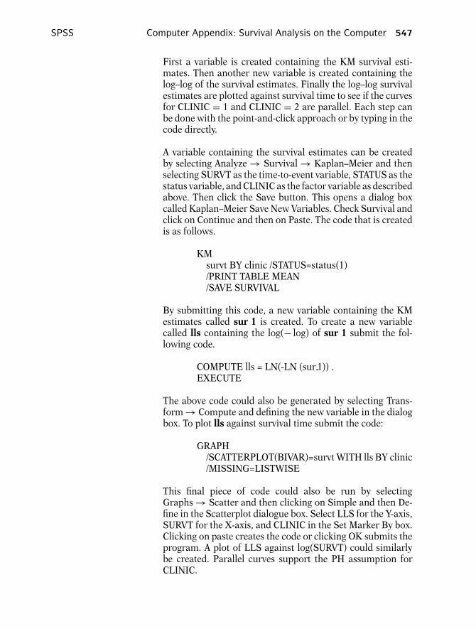
SPSS Computer Appendix: Survival Analysis on the Computer 547
First a variable is created containing the KM survival esti-mates. Then another new variable is created containing thelog–log of the survival estimates. Finally the log–log survivalestimates are plotted against survival time to see if the curvesfor CLINIC = 1 and CLINIC = 2 are parallel. Each step canbe done with the point-and-click approach or by typing in thecode directly.
A variable containing the survival estimates can be createdby selecting Analyze → Survival → Kaplan–Meier and thenselecting SURVT as the time-to-event variable, STATUS as thestatus variable, and CLINIC as the factor variable as describedabove. Then click the Save button. This opens a dialog boxcalled Kaplan–Meier Save New Variables. Check Survival andclick on Continue and then on Paste. The code that is createdis as follows.
KMsurvt BY clinic /STATUS=status(1)/PRINT TABLE MEAN/SAVE SURVIVAL
By submitting this code, a new variable containing the KMestimates called sur 1 is created. To create a new variablecalled lls containing the log(− log) of sur 1 submit the fol-lowing code.
COMPUTE lls = LN(-LN (sur-1)) .EXECUTE
The above code could also be generated by selecting Trans-form → Compute and defining the new variable in the dialogbox. To plot lls against survival time submit the code:
GRAPH/SCATTERPLOT(BIVAR)=survt WITH lls BY clinic/MISSING=LISTWISE
This final piece of code could also be run by selectingGraphs → Scatter and then clicking on Simple and then De-fine in the Scatterplot dialogue box. Select LLS for the Y-axis,SURVT for the X-axis, and CLINIC in the Set Marker By box.Clicking on paste creates the code or clicking OK submits theprogram. A plot of LLS against log(SURVT) could similarlybe created. Parallel curves support the PH assumption forCLINIC.
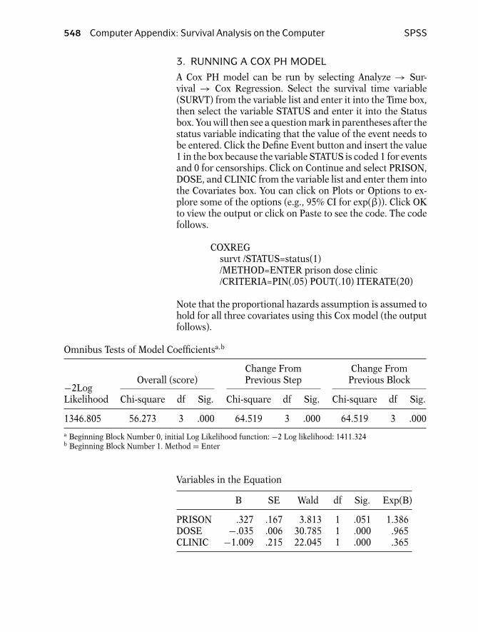
548 Computer Appendix: Survival Analysis on the Computer SPSS
3. RUNNING A COX PH MODEL
A Cox PH model can be run by selecting Analyze → Sur-vival → Cox Regression. Select the survival time variable(SURVT) from the variable list and enter it into the Time box,then select the variable STATUS and enter it into the Statusbox. You will then see a question mark in parentheses after thestatus variable indicating that the value of the event needs tobe entered. Click the Define Event button and insert the value1 in the box because the variable STATUS is coded 1 for eventsand 0 for censorships. Click on Continue and select PRISON,DOSE, and CLINIC from the variable list and enter them intothe Covariates box. You can click on Plots or Options to ex-plore some of the options (e.g., 95% CI for exp(β)). Click OKto view the output or click on Paste to see the code. The codefollows.
COXREGsurvt /STATUS=status(1)/METHOD=ENTER prison dose clinic/CRITERIA=PIN(.05) POUT(.10) ITERATE(20)
Note that the proportional hazards assumption is assumed tohold for all three covariates using this Cox model (the outputfollows).
Omnibus Tests of Model Coefficientsa,b
Change From Change FromOverall (score) Previous Step Previous Block−2Log
Likelihood Chi-square df Sig. Chi-square df Sig. Chi-square df Sig.
1346.805 56.273 3 .000 64.519 3 .000 64.519 3 .000
a Beginning Block Number 0, initial Log Likelihood function: −2 Log likelihood: 1411.324b Beginning Block Number 1. Method = Enter
Variables in the Equation
B SE Wald df Sig. Exp(B)
PRISON .327 .167 3.813 1 .051 1.386DOSE −.035 .006 30.785 1 .000 .965CLINIC −1.009 .215 22.045 1 .000 .365

SPSS Computer Appendix: Survival Analysis on the Computer 549
4. RUNNING A STRATIFIED COX MODEL ANDOBTAINING COX ADJUSTED LOG–LOG CURVES
A stratified Cox model is run by selecting Analyze → Sur-vival → Cox Regression. Select the survival time variable(SURVT) from the variable list and enter it into the Time box.Select the variable STATUS and enter it into the Status boxand then define the value of the event as 1. Put the variablesPRISON and DOSE in the Covariates box and the variableCLINIC in the Strata box. The Cox model will be stratifiedby CLINIC. Click the Plots button and check Log minus logas the plot type and then click on Continue. Click on OK toview the output or click on Paste to see the code. The codefollows.
COXREGsurvt /STATUS=status(1) /STRATA=clinic/METHOD=ENTER prison dose/PLOT LML/CRITERIA=PIN(.05) POUT(.10) ITERATE(20)
The output containing the parameter estimates and the ad-justed log–log plots follows.
Variables in the Equation
B SE Wald df Sig. Exp(B)
PRISON .389 .169 5.298 1 .021 1.475DOSE −.035 .006 29.552 1 .000 .965
2
0
1
−1
−2
−6−200 0 200 400 600 800 1000
−5
−4
−3
Log
min
us
log
Survival time (days)
CLINIC
2.00
1.00
LML Functions at mean of covariates

550 Computer Appendix: Survival Analysis on the Computer SPSS
Notice that there are parameter estimates for PRISON andDOSE but not CLINIC because CLINIC is the stratified vari-able. The Cox adjusted log–log plots are fitted using the meanvalues of PRISON and DOSE and are used to evaluate the PHassumption for CLINIC.
Suppose rather than using the mean value of DOSE for the ad-justed log–log plots, you wish to obtain adjusted plots in whichDOSE = 70. Run the same code as before, up to clicking onthe Plots button and checking Log minus log as the plot type.Now click on DOSE(Mean) in the window called CovariateValues Plotted at. Type in the value 70 in the box underneathcalled Change Value and click on the button called Change.Now the variable in the window should be called DOSE(70)rather than DOSE(Mean). Click on Continue and then OK toview the output.
5. ASSESSING THE PH ASSUMPTION WITHA STATISTICAL TEST
SPSS does not easily accommodate a statistical test on theproportional hazards assumption using the Schoenfeld resid-uals. However, it can be programmed using several steps. Thesteps are as follows.
1. Run a Cox PH model to obtain the Schoenfeld residuals forall the covariates. These residuals are saved as new vari-ables in the working dataset.
2. Delete observations that were censored.3. Create a variable that contains the ranked order of survival
time. For example, the subject who had the fourth eventgets a value of 4 for this variable.
4. Run correlations on the survival rankings with the Schoen-feld residuals.
5. The p-value for testing whether the correlation is zero be-tween the ranked survival time and the covariate’s Schoen-feld residuals is the p-value for the statistical test that thePH assumption is violated. The null hypothesis is that thePH assumption is not violated.
First, run a Cox PH model with CLINIC, PRISON, and DOSE.Click on the Save button before submitting the model. A dia-log box appears that is called Cox Regression: Save New Vari-ables. Check Partial Residuals (under Diagnostics) and clickon Continue. This creates three new variables in the workingdataset called pr1 1, pr2 1, and pr3 1, which are the partialresiduals for CLINIC, PRISON, and DOSE, respectively. ClickOK to run the model (or Paste to generate the code).

SPSS Computer Appendix: Survival Analysis on the Computer 551
Next, delete all censored observations (i.e., only keep observa-tions in which STATUS = 1). To do this, select Data → SelectCases. Then check If condition is satisfied, and then click on If.Type status=1 in the dialog box and click on Continue. CheckDeleted in the box called Unselected Cases Are. Click OK andonly observations with events will be kept in the dataset.
Create the variable that contains the ranking of survival timesby selecting Transform → Ranked Cases. Select the survivaltime variable (SURVT) in the Variables box. Click on RankTypes, check Ranks, and click on Continue and then click onTies, check Mean, and click Continue. Click OK and a newvariable (called rsurvt) will be created containing the rankedsurvival time.
Finally, obtain correlations (and their p-values) between theranked survival and the Schoenfeld residuals. Select Ana-lyze → Correlate. → Bivariate. Move the ranked survival timevariable as well as the three partial residual variables into thevariable box. Check Pearson (for Pearson correlations) andTwo-tailed for a two-tail test of significance and click OK tosee the output. The code that is generated from these stepsfollows.
COXREGsurvt /STATUS=status(1)/METHOD=ENTER clinic prison dose/SAVE= PRESID/CRITERIA=PIN(.05) POUT(.10) ITERATE(20)
FILTER OFF.USE ALL.SELECT IF(status=1).EXECUTE
RANKVARIABLES=survt (A) /RANK /PRINT=YES/TIES=MEAN
CORRELATIONS/VARIABLES=rsurvt pr1-1 pr2-1 pr3-1/PRINT=TWOTAIL NOSIG/MISSING=PAIRWISE

552 Computer Appendix: Survival Analysis on the Computer SPSS
The output containing the correlations follows.
Correlations
Partial Partial PartialRANK of Residual Residual ResidualSURVT for CLINIC for PRISON for DOSE
RANK of Pearson Correlation 1 −.262∗∗ −.080 .077SURVT Sig. (2-tailed) — .001 .332 .347
N 150 150 150 150Partial Pearson Correlation −.262∗∗ 1 .010 .023
residual for Sig. (2-tailed) .001 — .904 .776CLINIC N 150 150 150 150
Partial Pearson Correlation −.080 .010 1 .171∗residual for Sig. (2-tailed) .332 .904 — .037PRISON N 150 150 150 150
Partial Pearson Correlation −.077 .023 .171∗ 1residual Sig. (2-tailed) .347 .776 .037 —for DO N 150 150 150 150
∗∗ Correlation is significant at the 0.01 level (2-tailed).∗ Correlation is significant at the 0.05 level (2-tailed).
The p-values for the correlations are the p-values for the PHtest. In the output, examine the row labeled RANK of SURVTSig(2-tailed). Notice that the null hypothesis is rejected forCLINIC (p = 0.001) but not for PRISON (p = 0.332 ) or DOSE(p = 0.347).
6. RUNNING AN EXTENDED COX MODEL
An extended Cox model with exactly one time-dependent co-variate can be run using the point and click approach. Sup-pose we want to include a time-dependent covariate DOSEtimes the log of survival time. This product term could beappropriate if the hazard ratio comparing any two levels ofDOSE monotonically increases (or decreases) over time. Se-lect Analyze → Survival → Cox w/ Time-Dep Cov. This opensa dialog box called Expression for T COV . The user defines atime-dependent variable (called T COV ) in this box. A vari-able T is included in the variable list. This is the variablethat represents time-varying survival (as opposed to SURVTwhich is an individual’s fixed time of event). We wish to de-fine T COV to be the log of T times DOSE. Enter the expres-sion LN(T )∗DOSE into the dialog box and click on the Modelbutton. Now run a Cox model that includes the covariates:PRISON, CLINIC, DOSE, and T COV . The code generated isas follows.

SPSS Computer Appendix: Survival Analysis on the Computer 553
TIME PROGRAM.COMPUTE T-COV-= LN(T-) ∗ dose
COXREGsurvt /STATUS=status(1)/METHOD=ENTER prison clinic dose T-COV-/CRITERIA=PIN(.05) POUT(.10) ITERATE(20)
The output containing the parameter estimates follows.
Variables in the Equation
B SE Wald df Sig. Exp(B)
PRISON .340 .167 4.134 1 .042 1.406CLINIC −1.019 .215 22.369 1 .000 .361DOSE −.082 .036 5.247 1 .022 .921T-COV- .009 .006 1.765 1 .184 1.009
The variable T COV represents the time-dependent variableincluded in the model, which in this example is DOSE timesthe log of survival time.
A Heaviside function for CLINIC can similarly be created. Wecan define a time-dependent variable equal to CLINIC if timeis greater than or equal to 365 days and 0 otherwise. SelectAnalyze → Survival → Cox w/ Time-Dep Cov. Define T COVto be (T ≥ 365)∗CLINIC. After clicking on the Model button,run a Cox model that includes PRISON, DOSE, CLINIC, andT COV . The code generated is as follows.
TIME PROGRAM.COMPUTE T-COV-= (T->= 365)∗ clinic
COXREGsurvt /STATUS=status(1)/METHOD=ENTER prison dose clinic T-COV-/CRITERIA=PIN(.05) POUT(.10) ITERATE(20)
Note that SPSS recognizes the expression (T >= 365) as tak-ing the value 1 if survival time is ≥ 365 days and 0 otherwise.

554 Computer Appendix: Survival Analysis on the Computer SPSS
The output follows.
Variables in the Equation
B SE Wald df Sig. Exp(B)
PRISON .378 .168 5.030 1 .025 1.459CLINIC −.460 .255 3.241 1 .072 .632DOSE −.036 .006 30.450 1 .000 .965T-COV- −1.369 .461 8.799 1 .003 .254
Notice the variable CLINIC is included in this model andthe time-dependent Heaviside function T COV does not con-tribute to the estimated hazard ratio until day 365. The esti-mated hazard ratio for CLINIC at 100 days is exp(−0.460) =0.632 and the estimated hazard ratio for CLINIC at 400 daysis exp((−0.460) + (−1.369)) = 0.161.
It may be of interest to define two Heaviside functions (withCLINIC) and not include CLINIC in the model. This is essen-tially the same model as the one described above with oneHeaviside function. However, the coding of two Heavisidefunctions makes it somewhat computationally more conve-nient for estimating the two hazard ratios for CLINIC (HRfor <365 days and HR for ≥365 days). Unfortunately, SPSSallows just one time-dependent variable (i.e., T COV ) usingthe point and click approach. However, by examining the codecreated for the single Heaviside function, there is only a slightadjustment needed to create code for two Heaviside functions.The following code creates two Heaviside functions (calledHV1 and HV2) and runs a model containing PRISON, DOSE,HV1, and HV2.
TIME PROGRAM.COMPUTE hv2= (T->= 365)∗ clinicCOMPUTE hv1= (T-< 365)∗ clinic
COXREGsurvt /STATUS=status(1)/METHOD=ENTER prison dose hv1 hv2/CRITERIA=PIN(.05) POUT(.10) ITERATE(20)

SPSS Computer Appendix: Survival Analysis on the Computer 555
The output follows.
Variables in the Equation
B SE Wald df Sig. Exp(B)
PRISON .378 .168 5.030 1 .025 1.459DOSE −.036 .006 30.450 1 .000 .965HV1 −.460 .255 3.241 1 .072 .632HV2 −1.828 .386 22.439 1 .000 .161
The parameter estimates for HV1 and HV2 can be used di-rectly to obtain the estimated hazard ratio for CLINIC = 2vs. CLINIC = 1 before and after 365 days. The estimatedhazard ratio for CLINIC at 100 days is exp(−0.460) = 0.632and the estimated hazard ratio for CLINIC at 400 days isexp(−1.828) = 0.161. These results are consistent with theestimates obtained from the previous model with one Heavi-side function.

TestAnswers
557
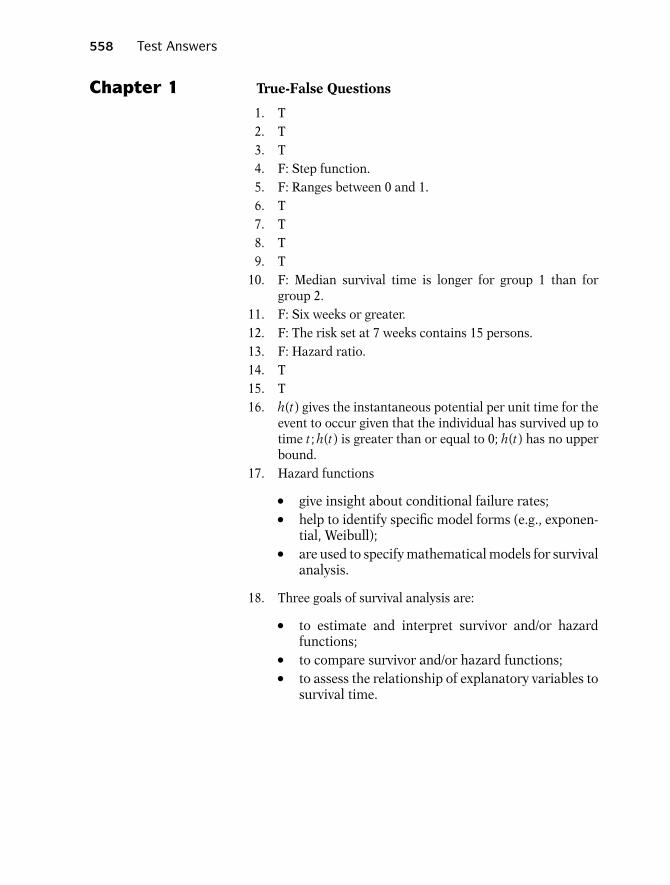
558 Test Answers
Chapter 1 True-False Questions
1. T2. T3. T4. F: Step function.5. F: Ranges between 0 and 1.6. T7. T8. T9. T
10. F: Median survival time is longer for group 1 than forgroup 2.
11. F: Six weeks or greater.12. F: The risk set at 7 weeks contains 15 persons.13. F: Hazard ratio.14. T15. T16. h(t) gives the instantaneous potential per unit time for the
event to occur given that the individual has survived up totime t; h(t) is greater than or equal to 0; h(t) has no upperbound.
17. Hazard functions
� give insight about conditional failure rates;� help to identify specific model forms (e.g., exponen-tial, Weibull);� are used to specify mathematical models for survivalanalysis.
18. Three goals of survival analysis are:
� to estimate and interpret survivor and/or hazardfunctions;� to compare survivor and/or hazard functions;� to assess the relationship of explanatory variables tosurvival time.
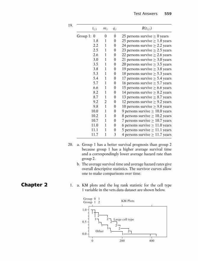
Test Answers 559
19.t( j ) mj q j R(t( j ))
Group 1: 0 0 0 25 persons survive ≥ 0 years1.8 1 0 25 persons survive ≥ 1.8 years2.2 1 0 24 persons survive ≥ 2.2 years2.5 1 0 23 persons survive ≥ 2.5 years2.6 1 0 22 persons survive ≥ 2.6 years3.0 1 0 21 persons survive ≥ 3.0 years3.5 1 0 20 persons survive ≥ 3.5 years3.8 1 0 19 persons survive ≥ 3.8 years5.3 1 0 18 persons survive ≥ 5.3 years5.4 1 0 17 persons survive ≥ 5.4 years5.7 1 0 16 persons survive ≥ 5.7 years6.6 1 0 15 persons survive ≥ 6.6 years8.2 1 0 14 persons survive ≥ 8.2 years8.7 1 0 13 persons survive ≥ 8.7 years9.2 2 0 12 persons survive ≥ 9.2 years9.8 1 0 10 persons survive ≥ 9.8 years
10.0 1 0 9 persons survive ≥ 10.0 years10.2 1 0 8 persons survive ≥ 10.2 years10.7 1 0 7 persons survive ≥ 10.7 years11.0 1 0 6 persons survive ≥ 11.0 years11.1 1 0 5 persons survive ≥ 11.1 years11.7 1 3 4 persons survive ≥ 11.7 years
20. a. Group 1 has a better survival prognosis than group 2because group 1 has a higher average survival timeand a correspondingly lower average hazard rate thangroup 2.
b. The average survival time and average hazard rates giveoverall descriptive statistics. The survivor curves allowone to make comparisons over time.
Chapter 2 1. a. KM plots and the log rank statistic for the cell type1 variable in the vets.data dataset are shown below.
0.0
0.5
1.0
0 200
Large cell type
KM Plots
400
Other
2
22
22
11
11
11
1
2
Group 0 1Group 1 2
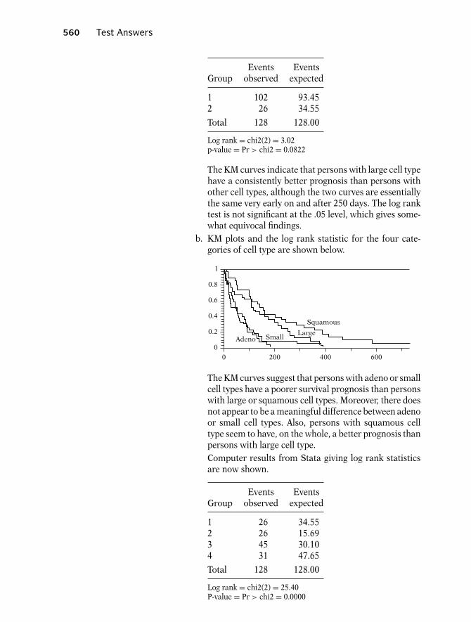
560 Test Answers
Events EventsGroup observed expected
1 102 93.452 26 34.55
Total 128 128.00
Log rank = chi2(2) = 3.02p-value = Pr > chi2 = 0.0822
The KM curves indicate that persons with large cell typehave a consistently better prognosis than persons withother cell types, although the two curves are essentiallythe same very early on and after 250 days. The log ranktest is not significant at the .05 level, which gives some-what equivocal findings.
b. KM plots and the log rank statistic for the four cate-gories of cell type are shown below.
0
0.2
0.4
0.6
0.8
1
0 200 400 600
LargeSmallAdeno
Squamous
The KM curves suggest that persons with adeno or smallcell types have a poorer survival prognosis than personswith large or squamous cell types. Moreover, there doesnot appear to be a meaningful difference between adenoor small cell types. Also, persons with squamous celltype seem to have, on the whole, a better prognosis thanpersons with large cell type.Computer results from Stata giving log rank statisticsare now shown.
Events EventsGroup observed expected
1 26 34.552 26 15.693 45 30.104 31 47.65
Total 128 128.00
Log rank = chi2(2) = 25.40P-value = Pr > chi2 = 0.0000
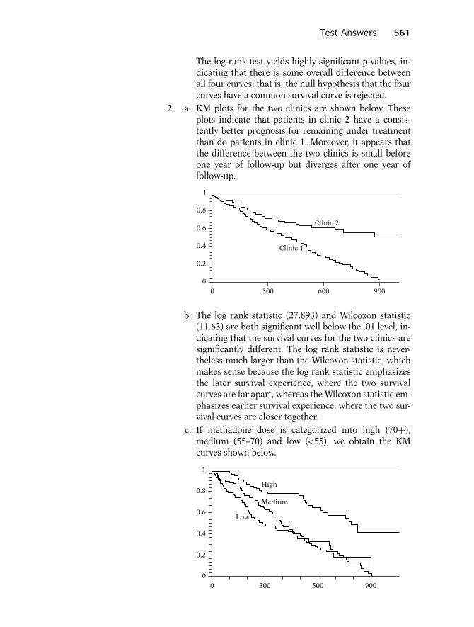
Test Answers 561
The log-rank test yields highly significant p-values, in-dicating that there is some overall difference betweenall four curves; that is, the null hypothesis that the fourcurves have a common survival curve is rejected.
2. a. KM plots for the two clinics are shown below. Theseplots indicate that patients in clinic 2 have a consis-tently better prognosis for remaining under treatmentthan do patients in clinic 1. Moreover, it appears thatthe difference between the two clinics is small beforeone year of follow-up but diverges after one year offollow-up.
0
0.2
0.4
0.6
0.8
1
0 300 600 900
Clinic 1
Clinic 2
b. The log rank statistic (27.893) and Wilcoxon statistic(11.63) are both significant well below the .01 level, in-dicating that the survival curves for the two clinics aresignificantly different. The log rank statistic is never-theless much larger than the Wilcoxon statistic, whichmakes sense because the log rank statistic emphasizesthe later survival experience, where the two survivalcurves are far apart, whereas the Wilcoxon statistic em-phasizes earlier survival experience, where the two sur-vival curves are closer together.
c. If methadone dose is categorized into high (70+),medium (55–70) and low (<55), we obtain the KMcurves shown below.
0
0.2
0.4
0.6
0.8
1
0 300 500 900
High
Medium
Low

562 Test Answers
The KM curves indicate that persons with high doses havea consistently better survival prognosis (i.e., maintenance)than persons with medium or low doses. The latter twogroups are not very different from each other, although themedium dose group has a somewhat better prognosis upto the first 400 days of follow-up.The log rank test statistic is shown below for the abovecategorization scheme.
Events EventsGroup observed expected
0 45 30.931 74 54.092 31 64.99
Total 150 150.00
Log rank = chi2(2) = 33.02P-value = Pr>chi2 = 0.0000
The test statistic is highly significant, indicating that thesethree curves are not equivalent.
Chapter 3 1. a. h(t,X) = h0(t) exp[β1T 1 + β2T2 + β3PS + β4DC+ β5BF + β6(T1 × PS) + β7(T2 × PS)+ β8(T1 × DC) + β9(T2 × DC)+ β10(T1 × BF) + β11(T2 × BF)]
b. Intervention A: X∗ = (1, 0, PS, DC, BF, PS, 0, DC, 0,BF, 0)Intervention C: X = (−1, −1, PS, DC, BF, −PS, −PS,−DC, −DC, −BF, −BF)
HR = h(t,X∗)h(t,X)
= exp[2β1 + β2 + 2β6PS + β7PS
+ 2β8DC + β9DC + 2β10BF
+ β11BF]
c. H0 : β6 = β7 = β8 = β9 = β10 = β11 = 0 in the fullmodel.Likelihood ratio test statistic: −2 ln L R − (−2 ln L F ),which is approximately χ2
6 under H0, where R denotesthe reduced model (containing no product terms) un-der H0, and F denotes the full model (given in Part 1aabove)
d. The two models being compared are:Full model (F ): h(t,X) = h0(t)exp[β1T1 + β2T2+ β3PS + β4DC + β5BF]

Test Answers 563
Reduced model (R): h(t,X) = h0(t)exp[β3PS+ β4DC + β5BF]H0: β1 = β2 = 0 in the full modelLikelihood ratio test statistic: −2 ln L R − (−2 ln L F ),which is approximately χ2
2 under H0.e.
Intervention A :
S(t,X) = [S0(t)]exp[β1+(PS)β3+(DC)β4+(BF)β5]
Intervention B :
S(t,X) = [S0(t)]exp[β2+(PS)β3+(DC)β4+(BF)β5]
Intervention C :
S(t,X) = [S0(t)]exp[−β1−β2+(PS)β3+(DC)β4+(BF)β5]
2. a. h(t,X) = h0(t)exp[β1 CHR + β2 AGE + β3(CHR ×AGE)]
b. H0: β3 = 0LR statistic = 264.90 − 264.70 = 0.21; χ2 with 1 d.f.under H0; not significant.Wald statistic gives a chi-square value of .01, also notsignificant. Conclusions about interaction: the modelshould not contain an interaction term.
c. When AGE is controlled (using the gold standard model2), the hazard ratio for the effect of CHR is exp(.8051) =2.24, whereas when AGE is not controlled, the haz-ard ratio for the effect of CHR (using Model 1) isexp(.8595) = 2.36. Thus, the hazard ratios are not ap-preciably different, so AGE is not a confounder.Regarding precision, the 95% confidence interval forthe effect of CHR in the gold standard model (Model2) is given by exp[.8051 ± 1.96(.3252)] = (1.183, 4.231)whereas the corresponding 95% confidence intervalin the model without AGE (Model 1) is given byexp[.8595 ± 1.96(.3116)] = (1.282, 4.350). Both confi-dence intervals have about the same width, with thelatter interval being slightly wider. Thus, controlling forAGE has little effect on the final point and interval esti-mates of interest.
d. If the hazard functions cross for the two levels of theCHR variable, this would mean that none of the modelsprovided is appropriate, because each model assumesthat the proportional hazards assumption is met foreach predictor in the model. If hazard functions crossfor CHR, however, the proportional hazards assumptioncannot be satisfied for this variable.

564 Test Answers
e. For CHR = 1: S(t,X) = [S0(t)]exp[0.8051+0.0856(AGE)]
For CHR = 0: S(t,X) = [S0(t)]exp[0.0856(AGE)]
f. Using Model 1, which is the best model, there is evi-dence of a moderate effect of CHR on survival time,because the hazard ratio is about 2.4 with a 95% con-fidence interval between 1.3 and 4.4, and the Wald textfor significance of this variable is significant below the.01 level.
3. a. Full model (F = Model 1): h(t,X) = h0(t) exp[β1 Rx+ β2Sex + β3 log WBC + β4(Rx × Sex)+ β5(Rx × log WBC)]Reduced model (R = model 4):h(t,X) = h0(t) exp[β1 Rx + β2Sex + β3 log WBC]H0: β4 = β5 = 0LR statistic = 144.218 − 139.030 = 5.19; χ2 with 2 d.f.under H0; not significant at 0.05, though significant at0.10. The chunk test indicates some (though mild) evi-dence of interaction.
b. Using either a Wald test (p-value = .776) or a LR test,the product term Rx × log WBC is clearly not signifi-cant, and thus should be dropped from Model 1. Thus,Model 2 is preferred to Model 1.
c. Using Model 2, the hazard ratio for the effect ofRx is given by: HR = (h(t,X∗))/(h(t,X)) = exp[0.405+ 2.013 Sex]
d. Males (Sex = 0): HR = exp[0.405] = 1.499Females (Sex = 1) : HR = exp[0.405 + 2.013(1)] =11.223
e. Model 2 is preferred to Model 3 if one decides thatthe coefficients for the variables Rx and Rx × Sex aremeaningfully different for the two models. It appearsthat such corresponding coefficients (0.405 vs. 0.587and 2.013 vs. 1.906) are different. The estimated haz-ard ratios for Model 3 are 1.799 (males) and 12.098 (fe-males), which are different, but not very different fromthe estimates computed in Part 3d for Model 2. If it isdecided that there is a meaningful difference here, thenwe would conclude that log WBC is a confounder; oth-erwise log WBC is not a confounder. Note that the logWBC variable is significant in Model 2 (P = .000), butthis addresses precision and not confounding. When indoubt, as in this case, the safest thing to do (for validityreasons) is to control for log WBC.
f. Model 2 appears to be best, because there is signifi-cant interaction of Rx × Sex (P = .023) and becauselog WBC is a likely confounder (from Part e).

Test Answers 565
Chapter 4 1. The P (PH) values in the printout provide GOF statisticsfor each variable adjusted for the other variables in themodel. These P (PH) values indicate that the clinic variabledoes not satisfy the PH assumption (P << .01), whereasthe prison and dose variables satisfy the PH assumption(P > .10).
2. The log–log plots shown are parallel. However, the reasonwhy they are parallel is because the clinic variable has beenincluded in the model, and log–log curves for any variablein a PH model must always be parallel. If, instead, the clinicvariable had been stratified (i.e., not included in the model),then the log–log plots comparing the two clinics adjustedfor the prison and dose variables might not be parallel.
3. The log–log plots obtained when the clinic variable isstratified (i.e., using a stratified Cox PH model) are not par-allel. They intersect early on in follow-up and diverge fromeach other later in follow-up. These plots therefore indi-cate that the PH assumption is not satisfied for the clinicvariable.
4. Both graphs of log–log plots for the prison variable showcurves that intersect and then diverge from each other andthen intersect again. Thus, the plots on each graph appearto be quite nonparallel, indicating that the PH assumptionis not satisfied for the prison variable. Note, however, thaton each graph, the plots are quite close to each other, sothat one might conclude that, allowing for random varia-tion, the two plots are essentially coincident; with this latterpoint of view, one would conclude that the PH assumptionis satisfied for the prison variable.
5. The conclusion of nonparallel log–log plots in Question 4gives a different result about the PH assumption for theprison variable than determined from the GOF tests pro-vided in Question 1. That is, the log–log plots suggest thatthe prison variable does not satisfy the PH assumption,whereas the GOF test suggests that the prison variable sat-isfies the assumption. Note, however, if the point of viewis taken that the two plots are close enough to suggest co-incidence, the graphical conclusion would be the same asthe GOF conclusion. Although the final decision is some-what equivocal here, we prefer to conclude that the PHassumption is satisfied for the prison variable because thisis strongly indicated from the GOF test and questionablycounterindicated by the log–log curves.
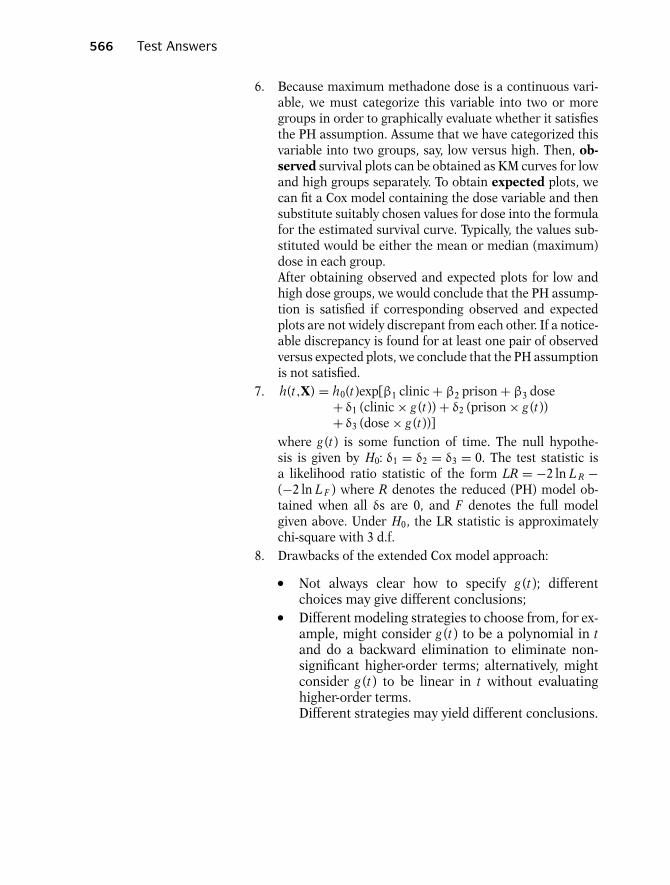
566 Test Answers
6. Because maximum methadone dose is a continuous vari-able, we must categorize this variable into two or moregroups in order to graphically evaluate whether it satisfiesthe PH assumption. Assume that we have categorized thisvariable into two groups, say, low versus high. Then, ob-served survival plots can be obtained as KM curves for lowand high groups separately. To obtain expected plots, wecan fit a Cox model containing the dose variable and thensubstitute suitably chosen values for dose into the formulafor the estimated survival curve. Typically, the values sub-stituted would be either the mean or median (maximum)dose in each group.After obtaining observed and expected plots for low andhigh dose groups, we would conclude that the PH assump-tion is satisfied if corresponding observed and expectedplots are not widely discrepant from each other. If a notice-able discrepancy is found for at least one pair of observedversus expected plots, we conclude that the PH assumptionis not satisfied.
7. h(t,X) = h0(t)exp[β1 clinic + β2 prison + β3 dose+ δ1 (clinic × g (t)) + δ2 (prison × g (t))+ δ3 (dose × g (t))]
where g (t) is some function of time. The null hypothe-sis is given by H0: δ1 = δ2 = δ3 = 0. The test statistic isa likelihood ratio statistic of the form LR = −2 ln L R −(−2 ln L F ) where R denotes the reduced (PH) model ob-tained when all δs are 0, and F denotes the full modelgiven above. Under H0, the LR statistic is approximatelychi-square with 3 d.f.
8. Drawbacks of the extended Cox model approach:
� Not always clear how to specify g (t); differentchoices may give different conclusions;� Different modeling strategies to choose from, for ex-ample, might consider g (t) to be a polynomial in tand do a backward elimination to eliminate non-significant higher-order terms; alternatively, mightconsider g (t) to be linear in t without evaluatinghigher-order terms.Different strategies may yield different conclusions.
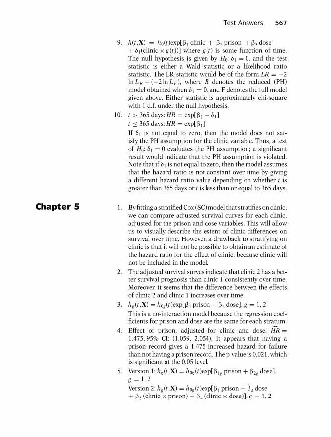
Test Answers 567
9. h(t,X) = h0(t)exp[β1 clinic + β2 prison + β3 dose+ δ1(clinic × g (t))] where g (t) is some function of time.The null hypothesis is given by H0: δ1 = 0, and the teststatistic is either a Wald statistic or a likelihood ratiostatistic. The LR statistic would be of the form LR = −2ln L R − (−2 ln L F ), where R denotes the reduced (PH)model obtained when δ1 = 0, and F denotes the full modelgiven above. Either statistic is approximately chi-squarewith 1 d.f. under the null hypothesis.
10. t > 365 days: HR = exp[β1 + δ1]t ≤ 365 days: HR = exp[β1]If δ1 is not equal to zero, then the model does not sat-isfy the PH assumption for the clinic variable. Thus, a testof H0: δ1 = 0 evaluates the PH assumption; a significantresult would indicate that the PH assumption is violated.Note that if δ1 is not equal to zero, then the model assumesthat the hazard ratio is not constant over time by givinga different hazard ratio value depending on whether t isgreater than 365 days or t is less than or equal to 365 days.
Chapter 5 1. By fitting a stratified Cox (SC) model that stratifies on clinic,we can compare adjusted survival curves for each clinic,adjusted for the prison and dose variables. This will allowus to visually describe the extent of clinic differences onsurvival over time. However, a drawback to stratifying onclinic is that it will not be possible to obtain an estimate ofthe hazard ratio for the effect of clinic, because clinic willnot be included in the model.
2. The adjusted survival surves indicate that clinic 2 has a bet-ter survival prognosis than clinic 1 consistently over time.Moreover, it seems that the difference between the effectsof clinic 2 and clinic 1 increases over time.
3. hg (t,X) = h0g (t)exp[β1 prison + β2 dose], g = 1, 2This is a no-interaction model because the regression coef-ficients for prison and dose are the same for each stratum.
4. Effect of prison, adjusted for clinic and dose: HR =1.475, 95% CI: (1.059, 2.054). It appears that having aprison record gives a 1.475 increased hazard for failurethan not having a prison record. The p-value is 0.021, whichis significant at the 0.05 level.
5. Version 1: hg (t,X) = h0g (t)exp[β1g prison + β2g dose],g = 1, 2Version 2: hg (t,X) = h0g (t)exp[β1 prison + β2 dose+ β3 (clinic × prison) + β4 (clinic × dose)], g = 1, 2

568 Test Answers
6. g = 1 (clinic 1) :h1(t,X) = h01(t)exp[(0.502)prison + (−0.036)dose]g = 2 (clinic 2) :h2(t,X) = h02(t)exp[(−0.083)prison + (−0.037)dose]
7. The adjusted survival curves stratified by clinic are virtu-ally identical for the no-interaction and interaction models.Consequently, both graphs (no-interaction versus interac-tion) indicate the same conclusion that clinic 2 has con-sistently larger survival (i.e., retention) probabilities thanclinic 1 as time increases.
8. H0: β3 = β4 = 0 in the version 2 model (i.e., the no-interaction assumption is satisfied). LR = −2 ln L R −(−2 ln L F ) where R denotes the reduced (no-interaction)model and F denotes the full (interaction) model. Underthe null hypothesis, LR is approximately a chi-square with2 degrees of freedom.Computed LR = 1195.428 − 1193.558 = 1.87; p-value =0.395; thus, the null hypothesis is not rejected and we con-clude that the no-interaction model is preferable to the in-teraction model.
Chapter 6 1. For the chemo data, the −log–log KM curves intersect ataround 600 days; thus the curves are not parallel, and thissuggests that the treatment variable does not satisfy the PHassumption.
2. The P (PH) value for the Tx variable is 0, indicating that thePH assumption is not satisfied for the treatment variablebased on this goodness-of-fit test.
3. h(t,X) = h0(t)exp[β1(T x)g1(t) + β2(T x)g2(t)
+ β3(T x)g3(t)]
where
g1(t) ={
1 if 0 ≤ t < 250 days0 if otherwise
g2(t) ={
1 if 250 ≤ t < 500 days0 if otherwise
g3(t) ={
1 if t ≥ 500 days0 if otherwise
4. Based on the printout the hazard ratio estimates andcorresponding p-values and 95% confidence intervals aregiven as follows for each time interval:
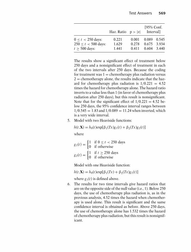
Test Answers 569
[95% Conf.Haz. Ratio p > |z| Interval]
0 ≤ t < 250 days: 0.221 0.001 0.089 0.545250 ≤ t < 500 days: 1.629 0.278 0.675 3.934t ≥ 500 days: 1.441 0.411 0.604 3.440
The results show a significant effect of treatment below250 days and a nonsignificant effect of treatment in eachof the two intervals after 250 days. Because the codingfor treatment was 1 = chemotherapy plus radiation versus2 = chemotherapy alone, the results indicate that the haz-ard for chemotherapy plus radiation is 1/0.221 = 4.52times the hazard for chemotherapy alone. The hazard ratioinverts to a value less than 1 (in favor of chemotherapy plusradiation after 250 days), but this result is nonsignificant.Note that for the significant effect of 1/0.221 = 4.52 be-low 250 days, the 95% confidence interval ranges between1/0.545 = 1.83 and 1/0.089 = 11.24 when inverted, whichis a very wide interval.
5. Model with two Heaviside functions:
h(t,X) = h0(t)exp[β1(Tx)g1(t) + β2(Tx)g2(t)]
where
g1(t) ={
1 if 0 ≤ t < 250 days0 if otherwise
g2(t) ={
1 if t ≥ 250 days0 if otherwise
Model with one Heaviside function:
h(t,X) = h0(t)exp[β1(Tx) + β2(Tx)g1(t)]
where g1(t) is defined above.6. The results for two time intervals give hazard ratios that
are on the opposite side of the null value (i.e., 1). Below 250days, the use of chemotherapy plus radiation is, as in theprevious analysis, 4.52 times the hazard when chemother-apy is used alone. This result is significant and the sameconfidence interval is obtained as before. Above 250 days,the use of chemotherapy alone has 1.532 times the hazardof chemotherapy plus radiation, but this result is nonsignif-icant.
570 Test Answers
Chapter 7 1. F: They are multiplicative models, although additive on thelog scale.
2. T3. T4. F: If the AFT assumption holds in a log-logistic model, the
proportional odds assumption holds.5. F: An acceleration factor greater than one suggests the ex-
posure is beneficial to survival.6. T7. T8. T9. F: ln(T) follows an extreme value minimum distribution.
10. F: The subject is right-censored.11.
γ = exp[α0 + α1(2) + α2PRISON + α3DOSE + α4PRISDOSE]exp[α0 + α1(1) + α2PRISON + α3DOSE + α4PRISDOSE]
= exp(α1)
γ = exp(0.698) = 2.01
95% CI = exp[0.698 ± 1.96(0.158)] = (1.47, 2.74)
The point estimate for the acceleration factor (2.01) sug-gests that the survival time (time off heroin) is double forthose enrolled in CLINIC = 2 compared to CLINIC = 1. The95% confidence interval does not include the null value of1.0 indicating a statistically significant preventive effect forCLINIC = 2 compared to CLINIC = 1.
12.HR = exp[β0 + β1(2) + β2PRISON + β3DOSE + β4PRISDOSE]
exp[β0 + β1(1) + β2PRISON + β3DOSE + β4PRISDOSE]
= exp(β1)
HR = exp(−0.957) = 0.38
95% CI = exp[−0.957 ± 1.96(0.213)] = (0.25, 0.58)
The point estimate of 0.38 suggests the hazard of goingback on heroin is reduced by a factor of 0.38 for thoseenrolled in CLINIC = 2 compared to CLINIC = 1. Or fromthe other perspective: the estimated hazard is elevated forthose in CLINIC = 1 by a factor of exp(+0.957) = 2.60.
13. β1 = −α1 p for CLINIC, so β1 = −(0.698)(1.370467) =−0.957, which matches the output for the PH form of themodel.
Test Answers 571
14. The product term PRISDOSE is included in the model asa potential confounder of the effect of CLINIC on survival.It is not an effect modifier because under this model thehazard ratio or acceleration factor for CLINIC does notdepend on the value of PRISDOSE. The PRISDOSE termwould cancel in the estimation of the hazard ratio or ac-celeration factor (see Questions 11 and 12). On the otherhand, a product term involving CLINIC would be a poten-tial effect modifier.
15. Using the AFT form of the model:
1
λ1/p= exp[α0 + α1CLINIC + α2PRISON + α3DOSE
+ α4PRISDOSE]Median survival time for CLINIC = 2, PRISON = 1, DOSE= 50, PRISDOSE = 100:
t = [− ln S(t)]1/p × 1
λ1/p= [− ln(0.5)]1/p
× exp[β0 + 2β1 + β2 + 50β3 + 100β4]
t (median) = 403.66 days (obtained by substituting param-eter estimates from output).
16. Using the same approach as the previous question:Median survival time for CLINIC = 1, PRISON = 1,DOSE = 50, PRISDOSE = 100:
t = [−ln(0.5)]1/p × exp[β0 + 1β1 + β2 + 50β3 + 100β4]
t (median) = 200.85 days.17. The ratio of the median survival times is 403.66/200.85 =
2.01. This is the estimated acceleration factor for CLINIC =2 vs. CLINIC = 1 calculated in Question 11. Note that if weused any survival probability (i.e., any quantile of survivaltime), not just S(t) = 0.5 (the median), we would have ob-tained the same ratio.
18. The addition of the frailty component did not change anyof the other parameter estimates nor did it change the loglikelihood of −260.74854.
19. If the variance of the frailty is zero (theta = 0), then thefrailty has no effect on the model. A variance of zero meansthe frailty (α) is constant at 1. Frailty is defined as a mul-tiplicative random effect on the hazard h(t|α) = αh(t). Ifα = 1 then h(t|α) = h(t), and there is no frailty.
572 Test Answers
Chapter 8 1. Cox PH Model for CP approach to Defibrillator Study:
h(t,X) = h0(t)exp[β tx + γ smoking]
where tx = 1 if treatment A, 0 if treatment B,smoking status = 1 if ever smoked, 0 if never smoked
2. Using the CP approach, there is no significant effect of treat-ment status adjusted for smoking. The estimated hazardratio for the effect of treatment is 1.09, the correspondingP-value is 0.42, and a 95% CI for the hazard ratio is (0.88,1.33).
3. No-interaction SC model for marginal approach:
hg(t,X) = h0g(t)exp[β tx + γ smoking], g = 1, 2, 3
Interaction SC model for marginal approach:
hg(t,X) = h0g(t)exp[βg tx + γg smoking], g = 1, 2, 3
4. LR = −2 ln LR − (−2 ln LF) is approximately χ2 with 4 dfunderH0: no-interaction SC model is appropriate, whereR denotes the reduced (no interaction SC) model andF denotes the full (interaction SC) model.
5. The use of a no-interaction model does not allow you toobtain stratum-specific HR estimates, even though you areassuming that strata are important.
6. The CP approach makes sense for these data because re-current defibrillator (shock) events on the same subject arethe same kind of event no matter when it occurred.
7. You might use the marginal approach if you determinedthat different recurrent events on the same subject weredifferent because they were of different order.
8. The number in the risk set (nj) remains unchanged throughday 68 because every subject who failed by this time wasstill at risk for a later event.
9. Subjects 3, 6, 10, 26, and 31 all fail for the third time at day98 and are not followed afterwards.
10. Subjects 9, 15, and 28 fail for the second time at 79 days,whereas subject #16 is censored at 79 days.
11. Subjects 4, 14, 15, 24, and 29 were censored between days111 and 112.
12. Subject #5 gets his first event at 45 days and his secondevent at 68 days, after which he drops out of the study. Thissubject is the first of the 36 subjects to drop out of the study,so the number in the risk set changes from 36 to 35 after68 days.

Test Answers 573
13. i. None of the above.ii. The product limit formula is not applicable to the CP
data; in particular, P(T > t | T ≥ t) does not equal “# fail-ing in time interval /# in the risk set at start of interval.”
14. Use the information provided in Table T.2 to complete thedata layouts for plotting the following survival curves.a. S1(t) = Pr(T1 > t) where T1 = time to first event from
study entry
t(j) nj mj qj S(t(j)) = S(t(j−1)) × Pr(T1 > t | T1 ≥ t)
0 36 0 0 1.0033 36 2 0 0.9434 34 3 0 0.8636 31 3 0 0.7837 28 2 0 0.7238 26 4 0 0.6139 22 5 0 0.4740 17 1 0 0.4441 16 1 0 0.4243 15 1 0 0.3944 14 1 0 0.3645 13 2 0 0.3146 11 2 0 0.2548 9 1 0 0.2249 8 1 0 0.1951 7 2 0 0.19 × 5/7 = 0.1457 5 2 0 0.14 × 3/5 = 0.0858 3 2 0 0.08 × 1/3 = 0.0361 1 1 0 0.03 × 0/1 = 0.00
b. Conditional S2c(t) = Pr(T2c > t) where T2c = time tosecond event from first event.
t(j) nj mj qj S(t(j)) = S(t(j−1)) × Pr(T1 > t | T1 ≥ t)
0 36 0 0 1.005 36 1 0 0.979 35 1 0 0.94
18 34 2 0 0.8920 32 1 0 0.8621 31 2 1 0.8123 28 1 0 0.7824 27 1 0 0.75
(Continued )

574 Test Answers
(Continued)
t(j) nj mj qj S(t(j)) = S(t(j−1)) × Pr(T1 > t | T1 ≥ t)
25 26 1 0 0.7226 25 2 0 0.6627 23 2 0 0.6028 21 1 0 0.5829 20 1 0 0.5530 19 1 0 0.5231 18 3 0 0.4332 15 1 0 0.4033 14 5 0 0.2635 9 1 0 0.2339 8 2 0 0.1740 6 2 0 0.17 × 4/6 = 0.1241 4 1 0 0.12 × 3/4 = 0.0942 3 1 0 0.09 × 2/3 = 0.0646 2 1 0 0.06 × 1/2 = 0.0347 1 1 0 0.03 × 0/1 = 0.00
c. Marginal S2m(t) = Pr(T2m > t) where T2m = time tosecond event from study entry.
t(j) nj mj qj S(t(j)) = S(t(j−1)) × Pr(T1 > t | T1 ≥ t)
0 36 0 0 1.0063 36 2 0 0.9464 34 3 0 0.8665 31 2 0 0.8166 29 3 0 0.7267 26 4 0 0.6168 22 2 0 0.5669 20 1 0 0.5370 19 1 0 0.5071 18 1 0 0.4772 17 2 0 0.4273 15 1 0 0.3974 14 1 0 0.3676 13 1 0 0.3377 12 1 0 0.3178 11 2 0 0.2579 9 3 1 0.25 × 6/9 = 0.1780 5 2 0 0.17 × 3/5 = 0.1081 3 2 0 0.10 × 1/3 = 0.0397 1 1 0 0.03 × 0/1 = 0.00

Test Answers 575
15. The survival curves corresponding to the above data lay-outs will differ because they are describing different sur-vival functions. In particular, the composition of the riskset differs in all three data layouts and the ordered survivaltimes being plotted are different as well.
Chapter 9 1. Cause-specific no-interaction model for local recurrence ofbladder cancer (event = 1):
h1(t,X) = h01(t)exp[β11tx + β21num + β31size]
2. Censored subjects have bladder metastasis (event = 2) orother metastasis (event = 3).
3. Cause-specific no-interaction model for bladder metastasis(event = 1):
h2(t,X) = h02(t)exp[β12tx + β22num + β32size]
where censored subjects have local recurrence of bladdercancer (event = 1) or other metastasis (event = 3).
4. A sensitivity analysis would consider worst-case violationsof the independence assumption. For example, subjectscensored from failing from events = 2 or 3 might be treatedin the analysis as either all being event-free (i.e., changeevent status to 0 and time to 53) or all experiencing theevent of interest (i.e., change event status to 1 and leavetime as is).
5. a. Verify the CIC1 calculation provided at failure timetj = 8 for persons in the treatment group (tx = 1):
h1(8) = 1/23 = 0.0435
S(4) = S(3)Pr(T > 4|T ≥ 4) = 0.9630(1 − 2/26)
= 0.9630(0.9231) = 0.8889
I1(8) = h1(8)S(4) = 0.0435(.8889) = 0.0387
CIC1(8) = CIC1(4) + 0.0387 = 0 + 0.0387 = 0.0387
b. Verify the CIC1 calculation provided at failure timetj = 25 for persons in the placebo group (tx = 0):
h1(25) = 1/6 = 0.1667
S(23) = S(21)Pr(T > 23|T ≥ 23) = 0.4150(1−1/8)
= 0.4150(0.875) = 0.3631
I1(25) = h1(25)S(23) = 0.1667(.3631) = 0.0605
CIC1(25) = CIC1(23) + 0.0605 = 0.2949 + 0.0605
= 0.3554
c. Interpret the CIC1 values obtained for both the treat-ment and placebo groups at tj = 30.For tx = 1, CIC1(tj = 30) = 0.3087 and for tx = 0,CIC1(tj = 30) = 0.3554.

576 Test Answers
Thus, for treated subjects (tx = 1), the cumulative risk(i.e., marginal probability) for local bladder cancer re-currence is about 30.1% at 30 months when allowing forthe presence of competing risks for bladder metastasisor other metastasis.For placebo subjects (tx = 1), the cumulative risk (i.e.,marginal probability) for local bladder cancer recur-rence is about 35.5% at 30 months when allowing forthe presence of competing risks for bladder metastasisor other metastasis.The placebo group therefore has a 5% increased risk offailure than the treatment group by 30 months of follow-up.
d. Calculating the CPC1 values for both treatment andplacebo groups at ti = 30:The formula relating CPC to CIC is given byCPCc = CICc/(1 − CICc′ ) where CICc = CIC for cause-specific risk event = 1 and CICc′ = CIC from risks forevents = 2 or 3 combinedFor tx = 1, CIC1(ti = 30) = 0.3087 and for tx = 0,
CIC1(tj = 30) = 0.3554.The calculation of CICc′ involves recoding the event vari-able to 1 for subjects with bladder metastasis or othermetastasis and 0 otherwise and then computing CICc′ .Calculation of CICc′ involves the following calculations.
tx = 1 (Treatment A)
tj nj d1j h 1(tj) S(tj−1) I1(tj) CIC1′ (tj)
0 27 0 0 — — —2 27 1 .0370 1 .0370 .03703 26 2 .0769 .9630 .0741 .11114 24 0 0 .8889 0 .11118 23 1 .0435 .8889 .0387 .14989 21 1 .0476 .8116 .0386 .1884
10 20 1 .0500 .7729 .0386 .227015 17 1 .0588 .7343 .0432 .270216 15 1 .0667 .6479 .0432 .313418 14 0 0 .6047 0 .313422 12 0 0 .6047 0 .313423 11 0 0 .5543 0 .313424 8 0 0 .5039 0 .313426 7 0 0 .4409 0 .313428 4 1 .2500 .3779 .0945 .407929 2 0 0 .2835 0 .407930 1 0 0 .2835 0 .4079
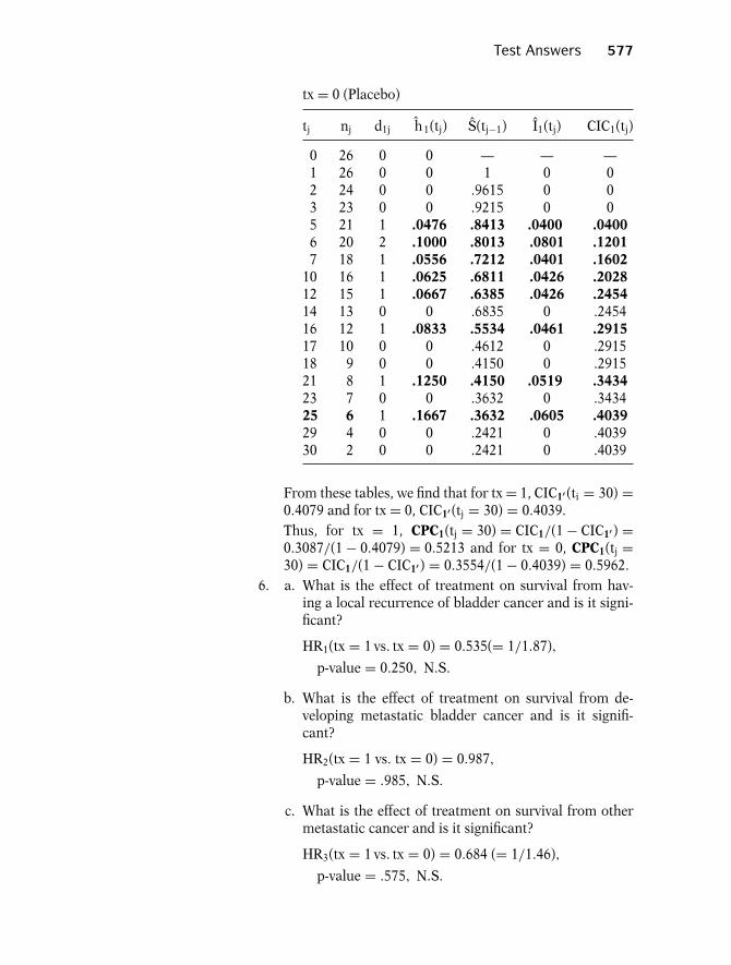
Test Answers 577
tx = 0 (Placebo)
tj nj d1j h 1(tj) S(tj−1) I1(tj) CIC1(tj)
0 26 0 0 — — —1 26 0 0 1 0 02 24 0 0 .9615 0 03 23 0 0 .9215 0 05 21 1 .0476 .8413 .0400 .04006 20 2 .1000 .8013 .0801 .12017 18 1 .0556 .7212 .0401 .1602
10 16 1 .0625 .6811 .0426 .202812 15 1 .0667 .6385 .0426 .245414 13 0 0 .6835 0 .245416 12 1 .0833 .5534 .0461 .291517 10 0 0 .4612 0 .291518 9 0 0 .4150 0 .291521 8 1 .1250 .4150 .0519 .343423 7 0 0 .3632 0 .343425 6 1 .1667 .3632 .0605 .403929 4 0 0 .2421 0 .403930 2 0 0 .2421 0 .4039
From these tables, we find that for tx = 1, CIC1′ (ti = 30) =0.4079 and for tx = 0, CIC1′ (tj = 30) = 0.4039.Thus, for tx = 1, CPC1(tj = 30) = CIC1/(1 − CIC1′ ) =0.3087/(1 − 0.4079) = 0.5213 and for tx = 0, CPC1(tj =30) = CIC1/(1 − CIC1′ ) = 0.3554/(1 − 0.4039) = 0.5962.
6. a. What is the effect of treatment on survival from hav-ing a local recurrence of bladder cancer and is it signi-ficant?
HR1(tx = 1 vs. tx = 0) = 0.535(= 1/1.87),
p-value = 0.250, N.S.
b. What is the effect of treatment on survival from de-veloping metastatic bladder cancer and is it signifi-cant?
HR2(tx = 1 vs. tx = 0) = 0.987,
p-value = .985, N.S.
c. What is the effect of treatment on survival from othermetastatic cancer and is it significant?
HR3(tx = 1 vs. tx = 0) = 0.684 (= 1/1.46),
p-value = .575, N.S.
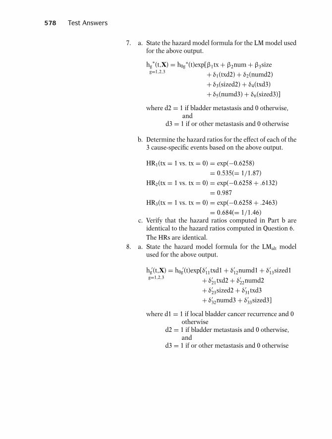
578 Test Answers
7. a. State the hazard model formula for the LM model usedfor the above output.
hg∗(t,X)
g=1,2,3= h0g
∗(t)exp[β1tx + β2num + β3size
+ δ1(txd2) + δ2(numd2)
+ δ3(sized2) + δ4(txd3)
+ δ5(numd3) + δ6(sized3)]
where d2 = 1 if bladder metastasis and 0 otherwise,and
d3 = 1 if or other metastasis and 0 otherwise
b. Determine the hazard ratios for the effect of each of the3 cause-specific events based on the above output.
HR1(tx = 1 vs. tx = 0) = exp(−0.6258)
= 0.535(= 1/1.87)
HR2(tx = 1 vs. tx = 0) = exp(−0.6258 + .6132)
= 0.987
HR3(tx = 1 vs. tx = 0) = exp(−0.6258 + .2463)
= 0.684(= 1/1.46)c. Verify that the hazard ratios computed in Part b are
identical to the hazard ratios computed in Question 6.The HRs are identical.
8. a. State the hazard model formula for the LMalt modelused for the above output.
hg′(t,X)
g=1,2,3= h0g
′(t)exp[δ′11txd1 + δ′
12numd1 + δ′13sized1
+ δ′21txd2 + δ′
22numd2
+ δ′23sized2 + δ′
31txd3
+ δ′32numd3 + δ′
33sized3]
where d1 = 1 if local bladder cancer recurrence and 0otherwise
d2 = 1 if bladder metastasis and 0 otherwise,and
d3 = 1 if or other metastasis and 0 otherwise

Test Answers 579
b. Determine the hazard ratios for the effect of each ofthe three cause-specific events based on the aboveoutput.
HR1(tx = 1 vs. tx = 0) = exp(−0.6258)
= 0.535 (= 1/1.87)
HR2(tx = 1 vs. tx = 0) = exp(−0.0127) = 0.987
HR3(tx = 1 vs. tx = 0) = exp(−0.3796)
= 0.684(= 1/1.46)
c. Verify that the hazard ratios computed in Part b areidentical to the hazard ratios computed in Questions 6and 7.Corresponding hazard ratios are identical.
9. State the formula for a no-interaction SC LM model forthese data.
h∗g(t,X)
g=1,2,3
= h∗0g(t)exp[β1tx + β2num + β8size]
Assumes HR1(X) = HR2(X) = HR3(X) for any X variablee.g., Rx = 0 vs. Rx = 1:HR1(tx) = HR2(tx) = HR3(tx) = exp[β1]
10. Describe how you would test whether a no-interaction SCLM model would be more appropriate than an interactionSC LM model.Carry out the following likelihood ratio test:
H0: δgj = 0, g = 2, 3; j = 1, 2, 3
where δgj is coefficient of DgXj in the interaction SC LMmodel
Likelihood Ratio test: LR = −2 log LR − (−2 log LF)approx χ2
6 under H0
R = no-interaction SC (reduced) modelF = interaction SC (full) model
References
Andersen, P.K., Borgan, O., Gill, R.D., and Keiding, N. 1993. Sta-tistical Models Based on Counting Processes. New York: Springer-Verlag.
AREDS Research Group. 2003. Potential public health impactof age-related eye disease study results. Arch. Opthamol. 121:1621–1624.
Byar, D. 1980. The Veterans Administration study of chemopro-phylaxis for recurrent stage I bladder tumors: Comparisons ofplacebo, pyridoxine, and topical thiotepa. In Bladder Tumors andOther Topics in Urological Oncology. New York: Plenum, 363–370.
Byar, D. and Green, S. 1980. The choice of treatment for cancerpatients based on covariate information. Bulletin du Cancer 67:4, 477–490.
Byar, D. and Corle, D. 1977. Selecting optimal treatment in clin-ical trials using covariate information. J. Chronic. Dis. 30: 445–459.
581

582 References
Caplehorn, J. et al. 1991. Methadone dosage and retention ofpatients in maintenance treatment. Med. J. Aust. 154: 195–199.
Clayton, D. 1994. Some approaches to the analysis of recurrentevent data. Stat. Meth. Med. Res. 3: 244–262.
Cox, D.R. and Oakes, D. 1984. Analysis of Survival Data. London:Chapman & Hall.
Crowley, J. and Hu, M. 1977. Covariance analysis of heart trans-plant data. J. Amer. Stat. Assoc. 72: 27–36.
Dixon, W.J. 1990. BMDP, Statistical Software Manual, Berkeley,CA: University of California Press.
Fine, J. and Gray, R. 1999. A proportional hazards model forthe subpopulation of a competing risk, J. Amer. Stat. Assoc. 94:496–509.
Freireich, E.O. et al. 1963. The effect of 6-mercaptopmine on theduration of steroid induced remission in acute leukemia. Blood,21: 699–716.
Gebski, V. 1997. Analysis of Censored and Correlated Data (AC-CORD). Eastwood, NSW, Australia: Data Analysis and ResearchTechnologies.
Grambsch, P.M. and Therneau, T.M. 1994. Proportional hazardstests and diagnostics based on weighted residuals. Biometrika81: 515–526.
Gray, R.J. 1988. A class of k-sample tests for comparingthe cumulative incidence of a competing risk. Ann. Stat. 16:1141–1154.
Gutierrez, R.G. 2002. Parametric frailty and shared frailty sur-vival models. Stata J. 2: 22–44.
Harrel, F. and Lee, K. 1986. Proceedings of the Eleventh AnnualSAS User’s Group International. 823–828.
Harris, E. and Albert, A. 1991. Survivorship Analysis for ClinicalStudies. New York: Marcel Dekker.
Hosmer, D.W. and Lemeshow, S. 1989. Applied Survival Analysis.New York: Wiley.

References 583
Kalbfleisch, J.D. and Prentice, R.L. 1980. The Statistical Analysisof Failure Time Data, New York: Wiley.
Kay, R. 1986. Treatment effects in competing-risk analysis ofprostate cancer data. Biometrics 42: 203–211.
Kleinbaum, D.G. and Klein, M. 2002. Logistic Regression—ASelf Learning Text, Second Edition. New York: Springer-Verlag,Chapter 11.
Kleinbaum, D.G., Kupper, L.L., and Morgenstern, H. 1982. Epi-demiologic Research: Principles and Quantitative Methods. NewYork: Van Nostrand Reinhold.
Kleinbaum, D.G., Kupper, L.L., and Muller, K.A. 1987. AppliedRegression Analysis and Other Multivariable Methods, SecondEdition. Belmont, CA: Wadsworth.
Krall, J.M., Uthoff, V.A., and Harley, J.B. 1975. A step-up pro-cedure for selecting variables associated with survival data.Biometrics. 31: 49–57.
Lee, E.T. 1980. Statistical Methods for Survival Data Analysis.Belmont, CA: Wadsworth.
Lin, D.Y. and Wei, L.J. 1989. The robust inference for the Coxproportional hazards model. J. Amer. Stat. Assoc. 84: 1074–1078.
Lunn, M. 1998. Applying k-sample tests to conditional probabil-ities for competing risks in a clinical trial. Biometrics 54: 1662–1672.
Lunn, M. and McNeil, D. 1995. Applying Cox regression to com-peting risks. Biometrics 51: 524–532.
Makuch, R.W. and Parks, W.P. 1988. Statistical methods for theanalysis of HIV-1 core polypeptide antigen data in clinical stud-ies. AIDS Res. Hum. Retroviruses 4: 305–316.
Pepe, M.S. and Mori, M. 1993. Kaplan–Meier, marginal or condi-tional probability curves in summarizing competing risks failuretime data? Stat. Med. 12: 737–751.
Prentice, R.L. and Marek. 1979. A qualitative discrepancy be-tween censored data rank tests. Biometrics 34.
584 References
Prentice, R.L., Williams, B.J. and Peterson, A.V. 1981. On theregression analysis of multivariate failure time data. Biometrika68 (2): 373–79.
Schoenbach, V.J., Kaplan, B.H., Fredman, L., and Kleinbaum,D.G. 1986. Social ties and mortality in Evans County, Georgia.Amer. J. Epid., 123:4, 577–591.
Schoenfeld, D. 1982. Partial residuals for the proportional haz-ards model. Biometrika, 69: 51–55.
Stablein, D., Carter, W., and Novak, J. 1981. Analysis of sur-vival data with non-proportional hazard functions. Control. Clin.Trials 2: 149–159.
Tai, B.C., Machin, D., White, I., and Gebski, V. 2001. Competingrisks analysis of patients with osteosarcoma: a comparison offour different approaches. Stat. Med. 20(5): 661–684.
Wei, L.J., Lin, D.Y., and Weissfeld, L. 1989. Regression analysis ofmultivariate incomplete failure time data by modeling marginaldistributions. J. Amer. Stat. Assoc. 84: 408.
Zeger, S.L. and Liang, C.Y. 1986. Longitudinal data analysis fordiscrete and continuous outcomes. Biometrics 42: 121–130.
Index
Accelerated failure time(AFT), see AFTentries
Acceleration factor, 266–267exponential, 269–271with frailty, 303, 309log-logistic, 281Weibull, 276
Addicts dataset, 464data analysis, 230–234,
248with SAS programming,
508–538with SPSS programming,
542–555with STATA
programming,467–502
Additive failure time model,285
Adjusted survival curves,104
log-log plots, 159observed versus expected
plots, 150stratified Cox procedure,
180using Cox PH model,
103–107, 116, 118AFT (accelerated failure
time) assumption,266–268
AFT models, 265–266,282–284, 309,313–317
Age–Related Eye DiseaseStudy (AREDS),359–364
AIC (Akaike’s informationcriterion), 286
585
586 Index
Average hazard rate, 24in Cox PH model, 94–95, 134in extended Cox model, 219in stratified Cox model, 181
Baseline hazard function, 94, 134Biased results, 405Binary regression, 290Bladder cancer dataset, 464–465Bladder cancer patients
comparison of results for, 355–357counting process for first 26
subjects, 339hypothetical subjects, 336–337interaction model results for, 354no-interaction model results for, 354
Byar data, 399–400cause-specific competing risk analysis,
401–403Lunn-McNeil models, 422, 427
Cause-specific hazard function, 400Censored data, 5–8
interval-censored, 286, 289left-censored, 7, 286right-censored, 7, 286
Censoring, 5non-informative (independent),
403–407informative (dependent), 405–406
CIC (cumulative incidence curves), 393,412–420
Competing risks, 4, 392, 396examples of data, 396–398CIC, 412CPC (Conditional Probability Curves),
420independence assumption, 403Lunn-McNeil models, 421, 427separate models for different event
types, 400–403Complementary log-log binary model, 293Complementary log-log link function, 292Computer
augmented (Lunn-McNeil approach)data layout for, 422
counting process data layout for,337–338
general data layout for, 15–19marginal approach data layout for,
348–349Conditional failure rate, 11Conditional probability curves (CPC),
420–421Conditional survival function, 295Confounding effect, 26–27Counting process (CP) approach, 334–336
example, 336–337general data layout, 338–344results for example, 346–347
Cox adjusted survival curvesusing SAS, 525–529using SPSS, 549–550using Stata, 485–488
Cox likelihood, 111–115extended for time dependent variables,
239–242Cox PH cause-specific model, 400Cox proportional hazards (PH) model
adjusted survival curves using,103–107
computer example using, 86–94extension of, see Extended Cox modelformula for, 94–96maximum likelihood estimation of,
98–100popularity of, 96–98review of, 214–216using SAS, 514–518using SPSS, 548using Stata, 476–481
CP, see Counting process approachCPC (conditional probability curves),
420–421Cumulative incidence, viiiCumulative incidence curves (CIC), 393,
412–420
Data layout for computer, 15–19Datasets, 464–465Decreasing Weibull model, 13Discrete survival analysis, 293
Index 587
Empirical estimation, 344Estimated -ln(-ln) survivor curves, 136Estimated survivor curves, 25Evans County Study,
Cox proportional hazards (PH) modelapplication to, 124–126
Kaplan-Meier survival curves for,73–75
multivariable example using, 29–31ordered failure times for, 41–42survival data from, 119–122
Event, 4Event types, different, separate models for,
400–403Expected versus observed plots, 145–150Exponential regression, 12
accelerated failure-time form, 319log relative-hazard form, 319
Extended Cox likelihood, 239–242Extended Cox model, 110, 219
application to Stanford hearttransplant data, 235–239
application to treatment of heroinaddiction, 230–234
hazard ratio formula for, 221–223using SAS, 530–533using SPSS, 552–555using Stata, 488–492time-dependent variables,
219–221
Failure, 4Failure rate, conditional, 11Flemington-Harrington test, 65Frailty component, 295Frailty effect, 300Frailty models, 294–308
using Stata, 499–502
Gamma distribution, 296Gamma frailty, 301Gastric carcinoma data, 253–254General stratified Cox (SC) model,
180–181Generalized gamma model, 284GOF, see Goodness-of-fit entries
Gompertz model, 285Goodness-of-fit (GOF) testing approach,
151–153Goodness-of-fit (GOF) tests, 136
Hazard function, 8, 9–10cause–specific, 400probability density function and,
262–263Hazard ratio, 32
formula fpr Cox PH model, 100–103formula for extended Coxmodel, 221–223
Heaviside function, 227
Increasing Weibull model, 13Independence assumption, 403–411Information matrix, 346Informative censoring, in competing
risks survival analysis, 405Instantaneous potential, 49Interactions, 27Interval-censored data, 286, 289–294Inverse-Gaussian distribution, 296
Kaplan-Meier (KM) curves, 46example of, 51–55general features of, 56–57log-log survival curves, 141
Left-censored data, 7–8, 286Leukemia remission-time data, 17, 26
Cox proportional hazards (PH) modelapplication to, 86–94
increasing Weibull for, 13Kaplan-Meier survival curves for,
51–55, 75–77log-log KM curves for, 141–145
recurrent event data for, 335exponential survival, 263–265stratified Cox (SC) model application
to, 176–188Likelihood function, 111–115
for Cox PH model,for extended Cox model, 239–242for parametric models, 286–289
588 Index
Likelihood ratio (LR) statistic, 89LM, see Lunn-McNeil approachLog-log plots, 137–145Log–log survival curves, 137–145Log-logistic regression, 277–282
accelerated failure-time form, 320Log-rank test, 46
alternatives to, 63–68for several groups, 61–63for two groups, 57–61
Logit link function, 292Lognormal survival models, 13, 284Lunn-McNeil (LM) approach, 393,
421–427alternative, 427–434
Macular degeneration data set, 359–364results for, 361–362Marginal probability, 414
Maximum likelihood (ML) estimation ofCox PH model, 98–100
Multiplicative model, 285
No-interaction assumption in stratifiedCox model, 182–188
Noninformative censoring, 403–407
Observed versus expected plots, 145–150
Parametric approach using shared frailty,357–359
Parametric survival models,defined, 260examples
exponential model, 263–265, 268–277log-logistic model, 277–282Weibull model, 272–277
likelihood function, 286–289other models, 284–286SAS use, 533–538Stata use, 492–499
Pepe-Mori test, 421, 437Peto test, 63PH assumption
assessment using time-dependentcovariates, 153–157, 224–229
evaluating (Chapter 4), 132–171meaning of, 107–111assessment using goodness of fit test
with Schonfield residuals, 151–153assessment using Kaplan-Meier log-log
survival curves, 546–547assessment using observed versus
expected plots, 145–150assessment using SAS, 522–525assessment using SPSS, 550–552assessment using Stata, 473–476,
483–485PH model, Cox, see Cox proportional
hazards (PH) modelPO (proportional odds) assumption, 292Precision, 92Probability, 11Probability density function, 262–263PROC LIFEREG (SAS), 533–538PROC LIFETEST (SAS), 510–514PROC PHREG, 514–518Product limit formula, 46Proportional hazards, see PH entriesProportional odds (PO) assumption, 292
Recurrent event survival analysis(Chapter 8), 332–390
Counting process approach, 336–344definition of recurrent events, 4, 332examples of recurrent event data,
334–336other approaches for analysis 347–353parametric approach using shared
frailty, 357–359SAS modeling, 538–542Stata modeling, 502–508survival curves with, 364–367
Right-censored data, 7, 286Risk set, 22Robust estimation, 344–346Robust standard error, 347Robust variance, 345
SAS, 508–542assessing PH assumption, with
statistical tests, 522–525

Index 589
demonstrating PROC LIFETEST,510–514
modeling recurrent events, 538–542obtaining Cox adjusted survival
curves, 525–529running Cox proportional hazards (PH)
model, with PROC PHREG,514–518
running extended Cox model, 530–533running parametric models, with PROC
LIFEREG, 533–538running stratified Cox (SC) model,
519–521SC, see Stratified Cox modelSchonfield residuals, 151–152, 522–523Score residuals, 346Semi-parametric model, 96, 261Sensitivity analysis (with competing
risks), 408–411Shape parameter, 272Shared frailty, 306–308, 358
recurrent events analysis using,357–359
Shared frailty model, 306SPSS, 542–555
assessing PH assumptionwith statistical tests, 550–552using Kaplan-Meier log-log survival
curves, 546–547estimating survival functions, 544–546running Cox proportional hazards (PH)
model, 548running extended Cox model, 552–555running stratified Cox (SC) model,
549–550Stanford Heart Transplant Study
extended Cox model application to,235–239
transplants versus nontransplants,244–245
Stata, 60, 465–508assessing PH assumption
using graphical approaches, 473–476using statistical tests, 483–485
estimating survival functions, 469–473modeling recurrent events, 502–508
obtaining Cox adjusted survival curveswith, 485–488
running Cox proportional hazards (PH)model, 476–481
running extended Cox model,488–492
running frailty models, 499–502running parametric models, 492–499running stratified Cox (SC) model,
481–483Step functions, 9Strata variable, 347Stratification variables, several, 188–193Stratified Cox (SC) model, 176–180,
364–367for analyzing recurrent event data,
347–353conditional approaches, 347–351general, 180–181graphical view of, 193–194marginal approach, 347–351using SAS, 519–521using SPSS, 549–550using Stata, 481–483 Subdistribution
function, 419Survival curves
adjusted, 104using Cox PH model, 103–107
Cox adjusted, see Cox adjustedsurvival curves
with recurrent events, 364–367Survival functions
conditional, 295probability density function and,
262–263SAS estimation, 525–529SPSS estimation, 544–546Stata estimation , 469–473unconditional, 295
Survival time, 4Survival time variable, 14Survivor function, 8–9
Tarone-Ware test statistic, 64Time-dependent covariates, assessing PH
assumption using, 153–157
590 Index
Time-dependent variables, 134definition and examples of, 216–219extended Cox model for, 219–221
Time-independent variables, PHassumption and, 224–229
Unconditional survival function, 295Unshared frailty, 306
Veterans Administration Lung CancerData
Kaplan–Meier survival curves for, 62–63model with no frailty, 296
proportional hazards assumptionevaluation for, 161–164
with several stratification variables,188–193
stratified Cox (SC) model applicationto, 201–204
Wald statistic, 89Weibull model, 272–277Weibull regression
accelerated failure-time form, 322, 325log relative-hazard form, 323, 325
Wilcoxon test, 64