statistics and topological data analysis · bertrand michel ecole centrale de nantes - lab. de math...
TRANSCRIPT

Bertrand MICHELEcole Centrale de Nantes - Lab. de mathematiques Jean Leray
Statistics and Topological Data Analysis
Geometry Understanding in Higher DimensionsCHAIRE D’INFORMATIQUE ET SCIENCES NUMERIQUES
College de France - June 2017

Introduction : Topological DataAnalysis and Statistics

Topological Data Analysis and Topological Inference
• The aim of TDA is to infer relevant qualitative and quantitative topologicalstructures (clusters, holes ...) directly from the data.
• Two popular methods in TDA : Mapper algorithm [Singh et al., 2007]and persistent homology [Edelsbrunner et al., 2002].
• data : typically point cloud Xn

Topological Data Analysis (TDA)
β0 β1 β2
topological space
point cloud
topological descriptors
Why is topology interesting for data analysis?
• multiscale
• compact
• invariant under coordinate changes
• stable with respect to (small) perturbations
• informative

• For exploratory analysis, visualization
Topological Data Analysis (TDA)

• For exploratory analysis, visualization
• For feature extraction and statistical learning
• Topological descriptors
• Geometric descriptors
• Other signatures
raw data • supervised methods
• unsupervised methods
Topological Data Analysis (TDA)

A statistical approach to TDA means that :
• we consider data as generated from an unknown distribution
• the inferred topological features by TDA methods are seen as estimatorsof topological quantities describing an underlying object.
Statistics, Learning and TDA
β0 β1 β2
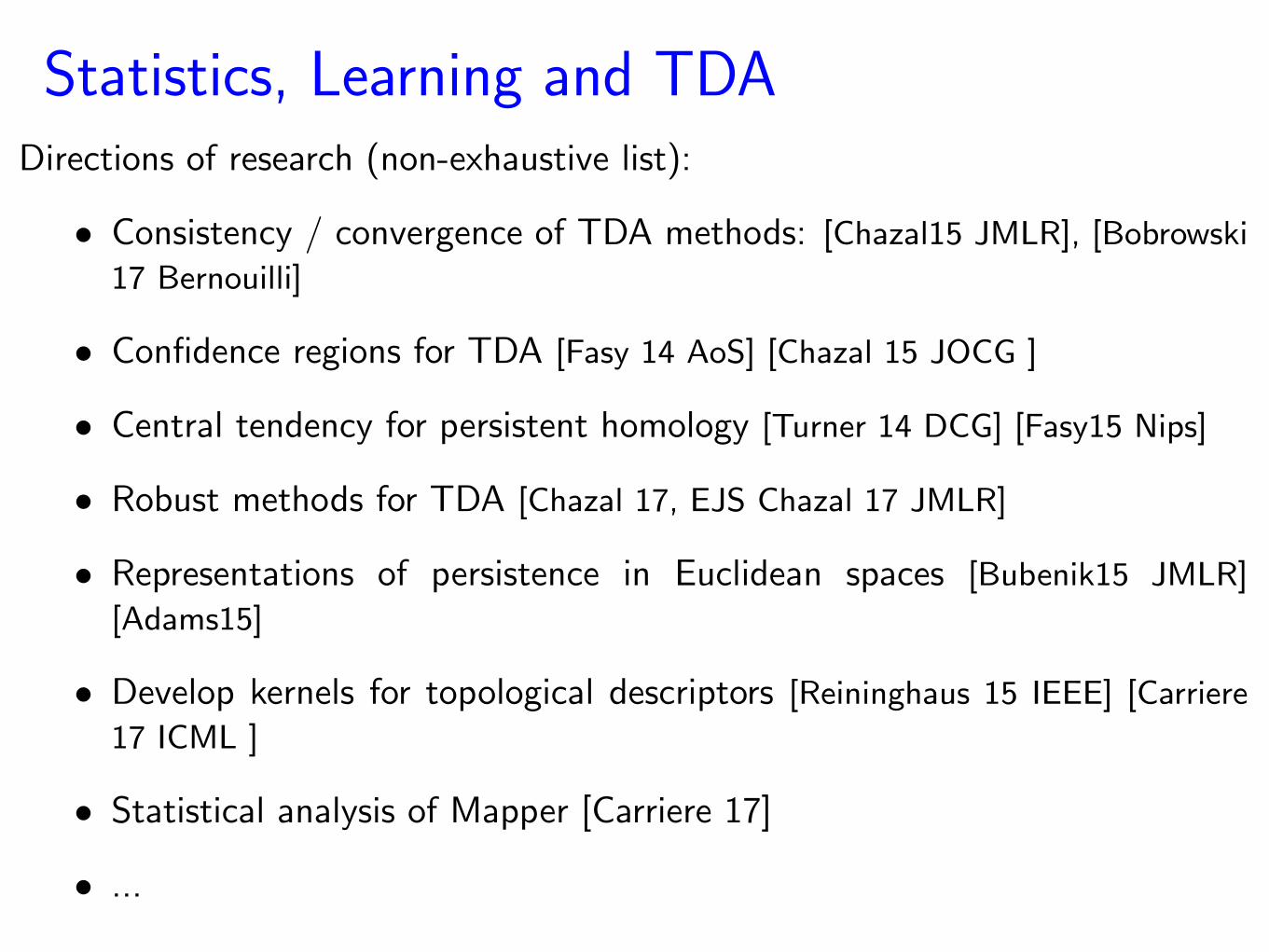
Directions of research (non-exhaustive list):
• Consistency / convergence of TDA methods: [Chazal15 JMLR], [Bobrowski
17 Bernouilli]
• Confidence regions for TDA [Fasy 14 AoS] [Chazal 15 JOCG ]
• Central tendency for persistent homology [Turner 14 DCG] [Fasy15 Nips]
• Robust methods for TDA [Chazal 17, EJS Chazal 17 JMLR]
• Representations of persistence in Euclidean spaces [Bubenik15 JMLR]
[Adams15]
• Develop kernels for topological descriptors [Reininghaus 15 IEEE] [Carriere
17 ICML ]
• Statistical analysis of Mapper [Carriere 17]
• ...
Statistics, Learning and TDA

Homologyand
Persistent homology
Topological Stability and Regularity
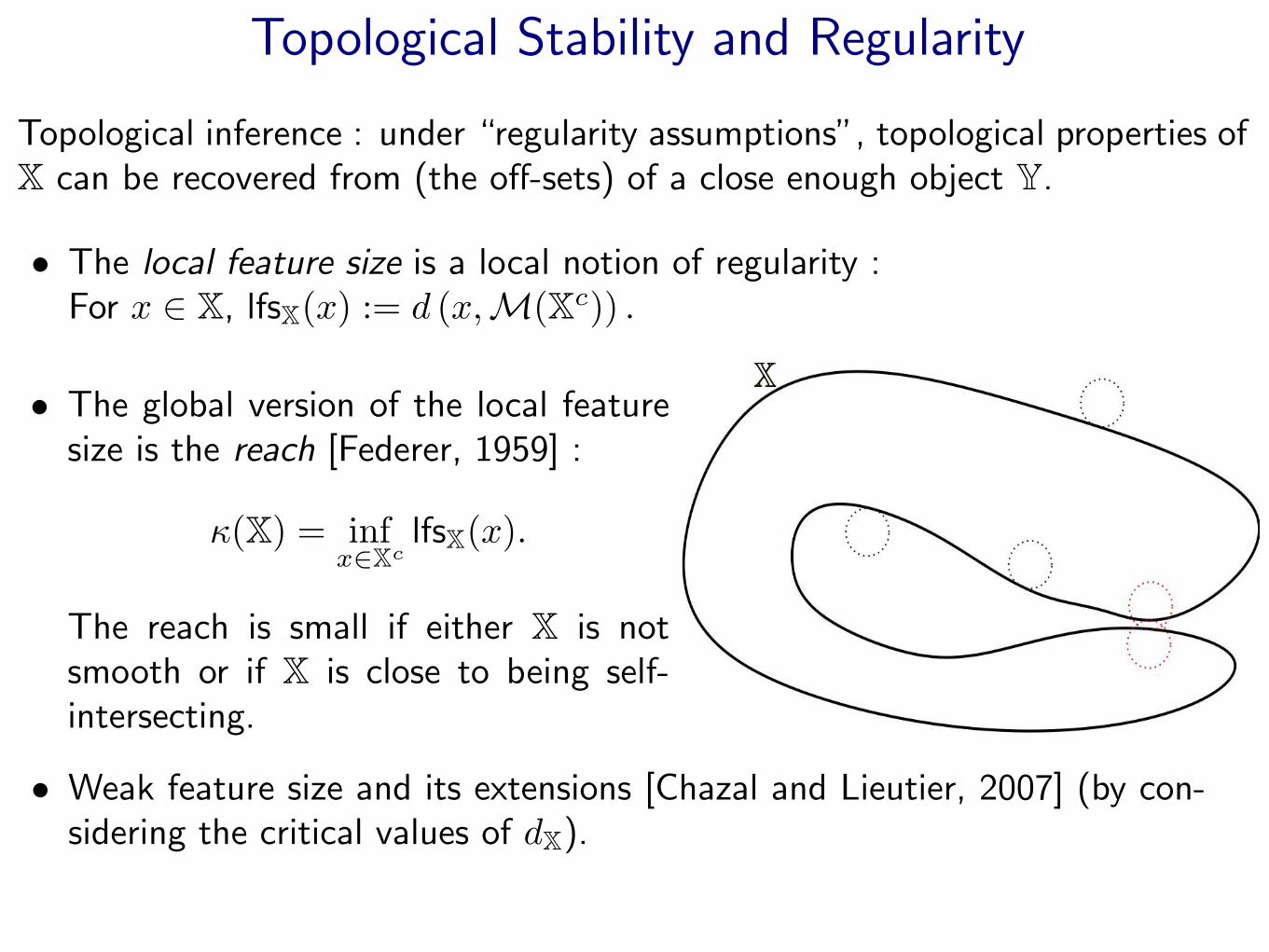
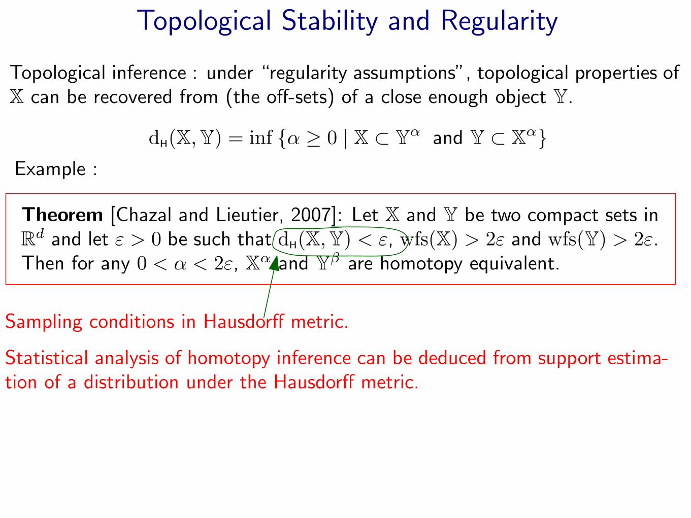
Topological inference : under “regularity assumptions”, topological properties ofX can be recovered from (the off-sets) of a close enough object Y.
Topological Stability and Regularity
Topological inference : under “regularity assumptions”, topological properties ofX can be recovered from (the off-sets) of a close enough object Y.
• The local feature size is a local notion of regularity :For x ∈ X, lfsX(x) := d (x,M(Xc)) .
• Weak feature size and its extensions [Chazal and Lieutier, 2007] (by con-sidering the critical values of dX).
• The global version of the local featuresize is the reach [Federer, 1959] :
κ(X) = infx∈Xc
lfsX(x).
The reach is small if either X is notsmooth or if X is close to being self-intersecting.

Topological Stability and Regularity
Topological inference : under “regularity assumptions”, topological properties ofX can be recovered from (the off-sets) of a close enough object Y.
Theorem [Chazal and Lieutier, 2007]: Let X and Y be two compact sets inRd and let ε > 0 be such that dH(X,Y) < ε, wfs(X) > 2ε and wfs(Y) > 2ε.Then for any 0 < α < 2ε, Xα and Yβ are homotopy equivalent.
Example :
dH(X,Y) = inf {α ≥ 0 | X ⊂ Yα and Y ⊂ Xα}
Sampling conditions in Hausdorff metric.
Statistical analysis of homotopy inference can be deduced from support estima-tion of a distribution under the Hausdorff metric.

Homology inference
• Homotopy is not easy to compute in practice.
• Singular homology provides a algebraic description of “holes” in a geo-metric shape (connected components, loops, etc ...)
• Betti number βk is the rank of the k-th homology group.
• Computational Topology : Betti numbers can be computed on simplicialcomplexes.
Homology inference [Niyogi et al., 2008 and 2011] [Balakrishnan et al., 2012] :The Betti number (actually the homotopy type) of Riemannian manifolds withpositive reach can be recovered with high probability from offsets of a sample on(or close to) the manifold.

Persistent homology
Starting from a point cloud Xn, let Filt = (Cα)α∈A be a fitration of nestedsimplicial complexes.
• multiscale information ;
• more stable and more robust ;
α
Persistent homology: identification of “persistent” topological features along thefiltration.

Barecodes and Persistence Diagrams
Xn
Barcode
Filtration of simplicialcomplexes Filt(Xn)
Offsets

Barecodes and Persistence Diagrams
Dgm (Filt(Xn))Persistence diagram of the
filtration Filt(Xn) built on Xn.
Xn
Barcode
Filtration of simplicialcomplexes Filt(Xn)
Offsets birth
death

Distance between persistence diagrams and stability
birth
death
∞
0
Multiplicity: 2
Add the diagonal
Dgm1
Dgm2
The bottleneck distance between two diagrams Dgm1 and Dgm2 is
db(Dgm1,Dgm2) = infγ∈Γ
supp∈Dgm1
‖p− γ(p)‖∞
where Γ is the set of all the bijections between Dgm1 and Dgm2 and
‖p− q‖∞ = max(|xp − xq|, |yp − yq|).

Distance between persistence diagrams and stability
birth
death
∞
0
Multiplicity: 2
Add the diagonal
Theorem [Chazal et al., 2012]: For any compact metric spaces (X, ρ) and (Y, ρ′),
db (Dgm(Filt(X)),Dgm(Filt(Y))) ≤ 2 dGH (X,Y) .
Consequently, if X and Y are embedded in the same metric space (M, ρ) then
db (Dgm(Filt(X)),Dgm(Filt(Y))) ≤ 2 dH (X,Y) .
Dgm(Filt(Y))
Dgm(Filt(X))

Statisticsand
Persistent homology

Persistence diagram inference [Chazal 2015 JMLR]
∞
00
Xn Filt(Xn)
Dgm(Filt(Xn))n points sampled in Xaccording to µ
Filt(X)
∞
00
Dgm(Filt(X))
X
Convergence???
Estimator of Dgm(Filt(K))
(M, ρ) metric spaceX compact set in M. well defined for any
compact metric space[Chazal et al., 2012]

Theorem: For a, b > 0 :
supµ∈P(a,b,M)
E[db(Dgm(Filt(Xµ)),Dgm(Filt(Xn)))
]≤ C
(lnn
n
)1/b
where C only depends on a and b.
Under additional technical hypotheses, for any estimator Dgmn of Dgm(Filt(Xµ)):
lim infn→∞
supµ∈P(a,b,M)
E[db(Dgm(Filt(Xµ)), Dgmn)
]≥ C′n−1/b
where C′ is an absolute constant.
For a, b > 0, µ satisfies the (a, b)-standard assumption on its support Xµ if for anyx ∈ Xµ and any r > 0 :
µ(B(x, r)) ≥ min(arb, 1).
P(a, b,M) : set of all the probability measures satisfying the (a, b)-standard as-sumption on the metric space (M, ρ).
Persistence diagram inference

Confidence sets for persistence diagrams [Fasy 2014 AoS]
P(
Dgm(Filt(K)) ∈ R)≥ 1− α ??

Confidence sets for persistence diagrams [Fasy 2014 AoS]
Using the Hausdorff stability, we can define confidence sets for persistence dia-grams:
db (Dgm (Filt(K)) ,Dgm (Filt(Xn))) ≤ dH(K,Xn).
It is sufficient to find cn such that
lim supn→∞
(dH(K,Xn) > cn
)≤ α.
P(
Dgm(Filt(K)) ∈ R)≥ 1− α ??

Confidence sets for persistence diagrams [Fasy 2014 AoS]
Subsampling method:
• N subsamples X1b,n, . . . ,XNb,n of size b.
• Compute Tj = dH
(Xjb,n,Xn
), j = 1, . . . , N .
• Compute Lb(t) = 1N
∑Nj=1 1Tj>t,
• Take cb = 2L−1b (α).
If P satisfies an (a, b) standard assumption then, for n large enough :
P(W∞ (Dgm (Filt(Xµ)) ,Dgm (Filt(Xn))) > cb
)≤ P
(dH (Xµ,Xn) > cb
)≤ α+O
(b
n
)1/4

Central tendency for persistent homology
• Frechet mean [Turner 2014]
• Use an alternative descriptor of persistence : Persistence landscapes[Bubenik, 2015]

Persistence landscapes [Bubnik JMLR 2015]
b
dd+b
2
d+b2
d−b2
Dgm ={
( di+bi2
, di+bi2
), i ∈ I} For p = ( b+d
2, d−b
2) ∈ Dgm,
Λp(t) =
t− b t ∈ [b, b+d
2]
d− t t ∈ ( b+d2, d]
0 otherwise.Persistence landscape λ of Dgm:
λ(k, t) = kmaxp∈D
Λp(t), t ∈ R, k ∈ N,
where kmax is k-th largest value in the set.
Stability: For any t ∈ R and any k ∈ N, |λ(k, t)− λ′(k, t)| ≤ db(Dgm,Dgm′).
Xn Dgm(Filt(Xn)) persistence landscape
d−b2

Subsampling methods for pers. homology [Chazal ICML 2015]
• Let X = {X1, · · · , Xm} sampled from µ.
• λX : corresponding persistence landscape.
• Ψmµ : the measure induced by µ⊗m on the space of persistence landscapes.
• We consider the point-wise expectations of the (random) persistence land-scape under this measure:
EΨmµ[λX(t)], t ∈ [0, T ]
• For Sm1 , . . . , Sm` some independent samples of size m from µ⊗m, the em-
pirical counterpart of EΨmµ[λX(t)] is
λm` (t) =1
`
∑i=1
λSmi (t), for all t ∈ [0, T ],
joint work with F. Chazal, B. Fasy, F. Lecci, A. Rinaldo and L. Wasserman

Subsampling methods for pers. homology [Chazal ICML 2015]
Theorem: Let X ∼ µ⊗m and Y ∼ ν⊗m, where µ and ν are two probabilitymeasures on M. For any p ≥ 1 we have∥∥∥EΨmµ
[λX ]− EΨmν[λY ]
∥∥∥∞≤ 2m
1pWρ,p(µ, ν).
Definition: The p-th Wasserstein distance between two measures µ, ν de-fined on (M, ρ) is
Wρ,p(µ, ν) =
(infΠ
∫M×M
[ρ(x, y)]pdΠ(x, y)
) 1p
,
where the infimum is taken over all measures on M ×M with marginals µand ν.
Stability of the average landscape:

Subsampling methods for pers. homology [Chazal ICML 2015]
Application: Analysis of accelerometer data.
• topological features carry discriminative information
• no registration/calibration preprocessing step needed
Fred
Fabrizio
Bertrand

and coming soon : Gudhi Stat with more tools for statistics and TDA.
Commercial break: Gudhi with Statistical learning Python Libraries

Robust TDA

Standard TDA methods are not robust to outliers
Xr :=⋃x∈X
B(x, r)
= d−1X ([0, r])
where the distancefunction dX to X is
dX(y) = infx∈X‖x− y‖

Standard TDA methods are not robust to outliers
Xr :=⋃x∈X
B(x, r)
= d−1X ([0, r])
where the distancefunction dX to X is
dX(y) = infx∈X‖x− y‖

Some possible “noise models” for geometry
• Additive noise model
• Clutter noise model
• A few outliers
P = µ ? Φ
distribution with supportthe geometric shape G
noise distribution
P = πµ+ (1− π)U
distribution with supportthe geometric shape G
Uniform distribu-tion on the box
P = πµ+ (1− π)Ψ
distribution with supportthe geometric shape G
Distribution of outliers
G
G
G

We would like to consider the sub levels of an alternative distance functionrelated to the sampling measure, which support is X, or close to X.
Robust TDA with an alternative distance function ?

Preliminary distance function to a measure P :Let u ∈]0, 1[ be a positive mass, and P a probability measure on Rd:
δP,u(x) = inf {r > 0 : P (B(x, r)) ≥ u}
supp(P )
x
δP,u(x)
u
δP,u is the smallest distance needed tocapture a mass of at least u.
δP,u is the quantile function at u of the r.v.
‖x−X‖
where X ∼ P .
Distance To Measure [Chazal 11 FoCM]

Preliminary distance function to a measure P :Let u ∈]0, 1[ be a positive mass, and P a probability measure on Rd:
δP,u(x) = inf {r > 0 : P (B(x, r)) ≥ u}
supp(P )
x
δP,u(x)
u
Definition: Given a probability measure Pon Rd and m > 0, the distance function tothe measure P (DTM) is defined by
dP,m : x ∈ Rd 7→(
1
m
∫ m
0
δ2P,u(x)du
)1/2
Distance To Measure [Chazal 11 FoCM]

Distance To Measure [Chazal 11 FoCM]
• Stability under Wassertein perturbations:
‖dP,m − dQ,m‖∞ ≤1√mW2(P,Q)
• The function x 7→ d2P,m(x) is semiconcave, this is ensuring strong reg-
ularity properties on the geometry of its sublevel sets.
• Consequently, if P is a probability distribution close to P for Wassersteindistance W2, then the sublevel sets of dP ,m provide a topologicallycorrect approximation of the support of P .
Properties of the DTM :

Let X1, . . . , Xn sample according to P and let Pn be the empirical measure.Then
d2Pn,
kn
(x) =1
k
k∑i=1
||x−X(i)||2
where ||X(1) − x|| ≥ ||X(2) − x|| ≥ · · · ≥ ||X(k) − x| · · · ≥ ||X(n) − x||
Distance to The Empirical Measure (DTEM)
x
k = 8
X(i)

Geometric inference with the DTM
Theorem: [Chazal et al., 2011]Let µ be a measure that has dimension at most k > 0 with compact supportG such that reachα(G) ≥ R > 0 for some α > 0.Let ν be another measure and ε be an upper bound on the uniform distancebetween dG and dν,m0 . Then, for any r ∈ [4ε/α2, R−3ε] and any η ∈]0, R[,the r-sublevel sets of dµ,m0 and the η-sublevel sets of dG are homotopyequivalent as soon as:
W2(µ, ν) ≤R√m0
5 + 4/α2− C(µ)−1/km
1/k+1/20 .
G
In practice : X1 . . . Xn sampled according to P .
Assume W2(P, µ) small.
Pn =∑ni=1 δXi : empirical measure.
Than for n large enough, W2(Pn, µ) is small and thesublevel sets of dPn,m provide a topologically correctapproximation of G.

Wasserstein deconvolution and DTM denoising
Additive noise model
P = µ ? Φ
distribution with supportthe geometric shape G
noise distribution G
In this case, W2(P, µ) can be large.
Ideally we would like to denoise directly dPn,n, but this can be hardly achievedbecause the DTM is not a linear functional of the measure.
Alternative approach : deconvolve the observed measure [Caillerie EJS 2011]
X1, . . . , Xn Deconvolvedmeasure µn
dµn,m
W2(Pn, µ) ≥W2(µn, µ) ≥√m‖dµn,m − dµ‖∞
(→ 0)(→ 0)

Wasserstein deconvolution and DTM denoising

DTM and persistent homology

DTM and persistent homology
db
(DgmP,m,DgmQ,m
)≤ ‖dP,m − dQ,m‖∞ ≤
1√mW2(P,Q)
Stability of Persistent homology [Cohen-Steiner et al.,2005, Chazal et al., 2012]
Wasserstein Stability of the DTM[Chazal et al., 2012]
Xi ∼ P
Take Q = Pn ...
dP,m
birth
death
∞
0
DgmP,m

Estimation of the DTM via the empirical DTM
Quantity of interest:d2Pn,
kn
(x)− d2P, kn
(x)
• Observe that
d2P,m(x) =
1
m
∫ m
0
F−1x (u)du
where Fx is the cdf of ‖x−X‖2 with X ∼ P .
• The distance to the empirical measure is the empirical counter part ofthe distance to P :
dPn,m(x)2 =1
m
∫ m
0
F−1x,n(u)du
where Fx,n is the cdf of ‖x−X‖2 with X ∼ Pn.
• Finally we get that
d2Pn,
kn
(x)− d2P, kn
(x) =1
m
∫ m
0
{F−1x,n(u)− F−1
x (u)}du
[Chazal EJS 17, Chazal JMLR 17]

Estimation of the DTM via the empirical DTM
Quantity of interest:d2Pn,
kn
(x)− d2P, kn
(x)
Two complementary approaches of the problem:
• Asymptotic approach : knn = m is fixed and n tends to infinity.
• Non asymptotic approach : n is fixed, and we want a tight controlover the fluctuations of the empirical DTM, in function of k, whichcan be taken very small.
We do not use Wasserstein stability for either of the two approaches.Wasserstein rates of convergence [Fournier and Guillin, 2013 ;Dereich et al.,2013] do not provide tight rates for the DTM in this context.
[Chazal EJS 17, Chazal JMLR 17]

Bootstrap and significance of topological features
Aim : studying the persistent homology of the sub-levels of the DTM andproviding confidence regions.
Two alternative boostrap methods :
• by bootstrapping the DTM
• Bottleneck Bootstrap

Bootstrap and significance of topological features
Bootstrapping the DTM
P
Pn

Bootstrap and significance of topological features
Bootstrapping the DTM
P
Pn
Pn
Bootstrapping the DTM
P ∗n

Bootstrap and significance of topological features
Bootstrapping the DTM
P
Pn
Pn
Bootstrapping the DTM
P ∗n

Bootstrap and significance of topological features
Bootstrapping the DTM
P
Pn
Pn
Bootstrapping the DTM
P ∗n
Φ(P )
Φ(Pn)
Φ(Pn)
Φ(P ∗n)

Bootstrap and significance of topological features
Bootstrapping the DTM
For m ∈ (0, 1), define cα by
P(√n||d2
P,m − d2Pn,m||∞ > cα
)= α.
Let X∗1 , . . . , X∗n be a sample from Pn, and let P ∗n be the corresponding (boot-
strap) empirical measure.
We consider the bootstrap quantity dP∗n ,m(x) of dPn,m.
The bootstrap estimate cα is defined by
P(√
n||d2Pn,m − d
2P∗n ,m
||∞ > cα |X1, . . . , Xn
)= α
where cα can be approximated by Monte Carlo.
Theorem: If F−1x is regular enough, the DTM is Hadamard differentiable at
P . Consequently, the bootstrap method for the DTM is asymptotically valid.

Bootstrap and significance of topological features
Dgm : persistence diagram of the sub-levels of dP,m
Dgm : persistence diagram of the sub-levels of dPn,m.Let
Cn =
{E ∈ Diag : db(Dgm, E) ≤ cα√
n
},
where Diag is the set of all the persistence diagrams.
Then,
P(Dgm ∈ Cn) = P(
db(Dgm, Dgm) ≤ cα√n
)≥ P
(‖d2P,m − d2
Pn,m‖∞ ≤cα√n
)
Bootstrapping the DTM
Bootstrap estimate

Bootstrap and significance of topological features
The Bottleneck Bootstrap
Dgm : persistence diagram of the sub-levels of dP,m
Dgm : persistence diagram of the sub-levels of dPn,m.
Dgm∗
: persistence diagram of the sub-levels of dP∗n ,m.
We directly bootstrap in the set of the persistence diagram by considering the
random quantity db(Dgm∗, Dgm). We define tα by
P(√
ndb(Dgm∗, Dgm) > tα |X1, . . . , Xn
)= α.
The quantile tα can be estimated by Monte Carlo.

Bootstrap and significance of topological features
In practice, the bottleneck bootstrap can lead to more precise inferences becausein many cases the stability result is not sharp enough:
db(Dgm,Dgm) ≤ ‖dP,m − dPn,m‖∞.
For both methods we can identify significant features by putting a bandof size 2cα or 2tα around the diagonal:

Concluding remarks
• TDA methods focus on the topological properties (homology / persistenthomology) of a shape.
• TDA methods can be used
– as an “exploratory method”, in particuar when the point cloud issampled on (close to) a real geometric object
– as a “feature extraction” procedure, next these extracted features canbe used for learning purposes.
• TDA is an emerging field, at the interface maths, computer sciences, statis-tics.
• Many topics about the statistical analysis of TDA
• Applications in many fields of sciences ( medecine, biology, dynamic sys-tems, astronomy, dynamical systems, physics ...)