statistics and data analysis
TRANSCRIPT

Final Project for Math 240 - MBA
Gangming Liang (Leon)
GGU ID #
0555970
1

Math 240
Final Project
Instructor: T. J. Tabara
Date 8/16/2010
Table of Contents
Abstract ……………………………………………………………………………………3
Objectives …………………………………………………………………………………3
Methods ……………………………………………………………………………………3
Overall Strategy …………………………………………………………………………3
Procedure …………………………………………………………………………………4
(1) EDA (Exploratory Data Analysis) ……………………………………………………4
(2) Scatter diagrams ………………………………………………………………………5
(3) Test on Linear Relationship by P- value Approach (Simple Regression) …………7
(4) Examine Regression Statistics …………………………………………………………7
(5) Regression Equation ……………………………………………………………………8
(6) Use Some Points for X to See How Good the Predicted Value ŷ are ………………8
(7) Best Fit Model - Linear Analysis ………………………………………………………9
1) Linearity2) Independence of Error
2

3) Normality 4) Equal variance:
Multiple Regression
(1) Overall F- test …………………………………………………………………………11
1) Examine R Square ……………………………………………………………………11
2) Test on Linear Relationship ……………………………………………………………11
(2) Individual T- Test ………………………………………………………………………12
(3) Regression Equation……………………………………………………………………12
(4) Residual Analysis - Line Analysis ……………………………………………………13
1) Linearity and Equal Variance2) Normality3) Independence
(5) Interaction Term with Ranking (X1) and Placement Success Rank (X4) …………15
(6) The Best Model …………………………………………………………………………15
Conclusions ………………………………………………………………………………16
Abstract:In order to find out the best model to estimate or predict salary/ bonus of MBA school, we
use simple linear regression and multiple regressions to test variables. In this process, we can know how well the population is explained by the regressions based on the result from Excel and PHStat. By comparing the r square and p- value of each model, we will find the minimum set of variables for estimating or predicting salary/ bonus. The regression equation of the best fit model must have the highest r square.
Objectives:1) Study how variables contribute the estimation of salary/ bonus2) Know how these variables related to each other3) Find out which is the best model4) Know how much of the population can b explained by the model
3

5) Develop a good method for getting the minimum set of variables which are all contribute to the model
6) Be familiar with operating Word, Excel, and PHStat
Methods:Exploratory Data AnalysisSimple Linear RegressionMultiple RegressionResidual AnalysisLine Analysis
Overall Strategy:First of all, we do an exploratory data analysis including numerical descriptive measures in
order to get a better understanding of distribution of the given data. Then, we construct scatter diagram to see how each variable relate to salary/ bonus. If some of them have a linear relationship with salary/ bonus, we choose one of them for simple regression. In the simple regression, we apply hypothesis test (p- value method) to determine if there is a linear relationship between observed variable and salary/ bonus.If there is a linear relationship, we will examine regression statistics to see how strong the relationship is and how much of the salary/ bonus in the population can be explained by ranking. Then, we get the regression equation for estimating salary/ bonus and use some points to see how good the predicted values are. Finally, a line analysis will be done to see if the model has good linearity, equal variance, independence, and normality. If all of them are good, the model is the best fit model; if not, it is not the best one. After doing a simple regression, we also need to do a multiple regression model. We will compare the overall F- test results of 3 combinations of independent variables to see which one explain the population at the highest r square. Then we choose the combination that has the highest r square for further analysis. Individual t- test will be done to each variable so that we can know if each variable contributes to the estimating model. If they all contribute to the model, we can say these variables work in the prediction of salary/ bonus together or individually. The next step is to get the regression equation and do residual analysis. A line analysis, including linearity, equal variance, independence, and normality, also has to be done to the model in order to see if it is the best fit model for estimating salary/ bonus of MBA school. In the final section, we will do an interaction term between a pair of variables to see if they have any interaction when contributing to the model. Based on the results of above analysis, we will decide the best regression equation of the best fit model for estimating salary/ bonus of MBA school.
Procedure:(1) EDA (Exploratory Data Analysis):
4
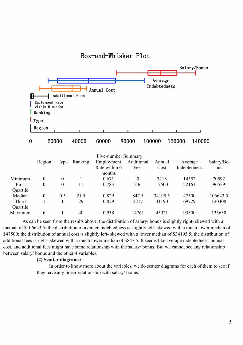
Box-and-Whisker Plot
Region
Type
Ranking
Employment Ratewithin 6 months
Additional Fees
Annual Cost
AverageIndebtedness
Salary/Bonus
0 20000 40000 60000 80000 100000 120000 140000
Five-number SummaryRegion Type Ranking Employment
Rate within 6 months
Additional Fees
Annual Cost
Average Indebtedness
Salary/Bonus
Minimum 0 0 1 0.671 0 7218 14352 70592First
Quartile0 0 11 0.783 236 17500 22161 96559
Median 0 0.5 21.5 0.829 847.5 34195.5 47500 106643.5Third
Quartile1 1 29 0.879 2217 41190 69729 120408
Maximum 6 1 40 0.938 14761 45921 93500 135630
As can be seen from the results above, the distribution of salary/ bonus is slightly right- skewed with a median of $106643.5; the distribution of average indebtedness is slightly left- skewed with a much lower median of $47500; the distribution of annual cost is slightly left- skewed with a lower median of $34195.5; the distribution of additional fees is right- skewed with a much lower median of $847.5. It seems like average indebtedness, annual cost, and additional fees might have some relationship with the salary/ bonus. But we cannot see any relationship between salary/ bonus and the other 4 variables.
(2) Scatter diagrams:In order to know more about the variables, we do scatter diagrams for each of them to see if
they have any linear relationship with salary/ bonus.
5

As can be seen, there seems that there is a negative linear correlation between placement success rank and salary/ bonus of MBA. However, there also seems some outliers, including Brigham Young University (Marriott) and Harvard University in the linear graph.
As can be seen, there seems insufficient evidence that there is a linear correlation between employment rate within 6 months and salary/ bonus of MBA. There appears no pattern on the graph as shown above.
As can be seen, there seems insufficient evidence that there is a linear correlation between region and salary/ bonus of MBA.
As can be seen, there seems insufficient evidence that there is a linear correlation between annual cost and salary/ bonus of MBA.
6

As can be seen, there seems insufficient evidence that there is a linear correlation between additional fees and salary/ bonus of MBA.
As can be seen, there seems insufficient evidence that there is a linear correlation between type and salary/ bonus of MBA.
As can be seen, there seems that there is a positive linear correlation between average indebtedness and salary/ bonus of MBA. As average indebtedness increase, salary/ bonus increase. However, the data from University of Florida and Columbia University appear to be outliers of the linear line.
As can be seen, there seems sufficient evidence that there is a negative linear correlation between ranking and salary/ bonus of MBA. The higher the ranking is, the lower the salary/ bonus are. But the data from Michigan State University and University of Maryland turn out to be outliers of the linear line.
As a result, placement success rank and ranking appear to have negative linear relationships with salary/ bonus; average indebtedness appears to have a positive linear relationship with salary/ bonus. However, only ranking has the strongest evidence that there us a linear relationship between ranking and salary/ bonus of MBA. So, we choose ranking to do a simple regression to see how much the ranking can explain in salary/ bonus of MBA school.
(3) Test on Linear Relationship by P- value Approach (Simple Regression):We set dependent variable y = salary/ bonus, independent variable x = ranking,
then we do a hypothesis test in order to see how strong the relationship between ranking and salary/ bonus.
H0: Relationship between ranking and salary/ bonus in the population = 0 (No linear relationship)
H1: Relationship between x and y in the population on is not equal to 0 (Linear relationship)
ANOVAdf F Significance F
SSR(Explained) 173.969985 2.36534E-15
7
1 6
We use p- value method to solve this problem, and we know significant level = 5%. And we also know p- value = Significance F = 2.36534E-15 = 0.00000000000000236534 from the result above. Then we get p- value< 5%.
Because in the bell- shaped distribution graph, p- value is the possibility that the observed object is not within 3 standard deviations. If p- value is lower than the significant level, the observed variable has linear relationship with salary/ bonus. If p- value is higher than the significant level, the observed variable is in the range of no linear relationship. In this case, the p- value is much lower than significant level 5%.
As a result, we reject H0. There is strong evidence that ranking and salary/ bonus are significantly linearly related. That is to say, the ranking in population are related to salary/ bonus of MBA schools.
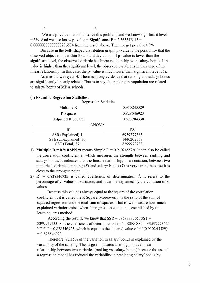
(4) Examine Regression Statistics:Regression Statistics
Multiple R 0.910245529
R Square 0.828546923
Adjusted R Square 0.823784338
ANOVAdf SS
SSR (Explained) 1 6959777365SSE (Unexplained) 36 1440202368
SST (Total) 37 8399979733
1) Multiple R = 0.910245529 means Simple R = 0.910245529. It can also be called the correlation coefficient r, which measures the strength between ranking and salary/ bonus. It indicates that the linear relationship, or association, between two numerical variables, ranking (X) and salary/ bonus (Y) is very strong because it is close to the strongest point, + 1.
2) R2 = 0.828546923 is called coefficient of determination r2. It refers to the percentage of y- values in variation, and it can be explained by the variation of x- values.
Because this value is always equal to the square of the correlation coefficient r, it is called the R Square. Moreover, it is the ratio of the sum of squared regression and the total sum of squares. That is, we measure how much explained variation exists when the regression equation is established by the least- squares method.
According the results, we know that SSR = 6959777365, SST = 8399979733. So the coefficient of determination is r2 = SSR/ SST = 6959777365/ 8399979733 = 0.828546923, which is equal to the squared value of r2 = (0.910245529)2
= 0.828546923.Therefore, 82.85% of the variation in salary/ bonus is explained by the
variability of the ranking. The large r2 indicates a strong positive linear relationship between two variables (ranking vs. salary/ bonus) because the use of a regression model has reduced the variability in predicting salary/ bonus by
8

82.85%. On the other hand, we can say that only 17.15% of the sample variability in salary/ bonus is due to factors other than what is accounted for by the linear regression model that uses ranking. These factors may be region, type of school, or employment rate within 6 months, etc.
3) Adjusted R2 = 0.823784338. It’s calculated by r2adj = 1- [(1- r2) (n- 1)/ (n-2)] = 1
- [(1- 0.9102455292) (38- 1)/ (38-2)] = 0.823784338. This helps us to remove data that are abnormal or special in the data sets. So, we could say that 82.38% of the variation in salary/ bonus is explained by the variability in the ranking.
(5) Regression Equation: Coefficients
Intercept (b0) 132638.3011Ranking (b1) -1195.02877
According to the result, b0 = 132638.3011 is Y- intercept, and b1 = -1195.02877 is the slope of the predicted line, and the linear regression equation is always of the form ŷ = b0 + b1 x (y is salary/ bonus, x is ranking). So, we can get the equation of linear regression line: ŷ = 132638.3011 - 1195. 02877 x.
The slope -1195.02877 means that for each of 1 unit X, i.e., each increase by 1 unit in ranking, the mean salary/ bonus is estimated to decrease by $1195.02877.The Y- intercept 132638.3011 is the point where the predicted line intercepts with the Y- axis (when X = 0). Theoretically, when the ranking is 0, the salary/ bonus is $132638.3011. This has obvious no practical interception. Considering the range of the observed values of the X variables (ranking), we must be careful when intercepting the value of b0.
(6) Use Some Points for X to See How Good the Predicted Value ŷ are:RESIDUAL OUTPUT
Observation Predicted Salary/Bonus Residuals14 131443.2723 3210.72769928 97982.46674 -4885.466737
Confidence Interval EstimateX Value 14 28Confidence Level 95% 95%Predicted Y (YHat) 115907.9 99177.5
If ranking is 14, then x = 14. So, we put x = 14 into the equation ŷ = 132638.3011 -1195.02877 x, and we get ŷ = 115907.9. This is the predicted salary/ bonus when the ranking is 14. In PHStat, we can find all the information about estimating a predicted value. According to the residual output, the predict value of salary/ bonus for ranking 14 is $131443.2723, and the residual is $3210.727699. This indicates the observation is above the predicted line.
Similarly, if x = 28, then ŷ = 99177.496. According to the residual output, the predict value of salary/ bonus for ranking 28 is $97982.46674, and the residual is -$4885.466737. This indicates the observation is above the predicted line.
9

(7) Best Fit Model:Linear Analysis:
Ranking Residual Plot
-25000
-20000
-15000
-10000
-5000
0
5000
10000
15000
20000
0 10 20 30 40 50
Ranking
Residuals
1) Linearity: After putting the residuals on the vertical axis against the corresponding X
values on the horizontal axis. If the linear model is appropriate for the data, there is no apparent pattern in the plot. In this case, however, there almost is an apparent pattern in the plot. The residuals don’t appear to be almost evenly spread above and below 0 for the differing value of X. For example, the data of University of Florida is an outlier of the linear line. So, there may be some non- linear relationship.
Residual Plot vs Time Period
-25000
-20000
-15000
-10000
-5000
0
5000
10000
15000
0 5 10 15 20 25 30 35 40
2) Independence of Error:We evaluate the assumption of independence of the errors by plotting the
residuals in the order in which the data were collected. If this relationship exists, it is apparent in the plot of the residuals versus time in which the data were collected. In this case, there is no relationship between consecutive residuals and time. That is to say, the residuals have no relationship with the time factor and they are all independent.
10
Normal Probability Plot
-25000
-20000
-15000
-10000
-5000
0
5000
10000
15000
20000
-2.5 -2 -1.5 -1 -0.5 0 0.5 1 1.5 2 2.5
Z Value
Residuals
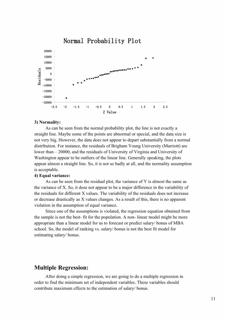
3) Normality:As can be seen from the normal probability plot, the line is not exactly a
straight line. Maybe some of the points are abnormal or special, and the data size is not very big. However, the data does not appear to depart substantially from a normal distribution. For instance, the residuals of Brigham Young University (Marriott) are lower than – 20000, and the residuals of University of Virginia and University of Washington appear to be outliers of the linear line. Generally speaking, the plots appear almost a straight line. So, it is not so badly at all, and the normality assumption is acceptable.4) Equal variance:
As can be seen from the residual plot, the variance of Y is almost the same as the variance of X. So, it dose not appear to be a major difference in the variability of the residuals for different X values. The variability of the residuals does not increase or decrease drastically as X values changes. As a result of this, there is no apparent violation in the assumption of equal variance.
Since one of the assumptions is violated, the regression equation obtained from the sample is not the best- fit for the population. A non- linear model might be more appropriate than a linear model for us to forecast or predict salary/ bonus of MBA school. So, the model of ranking vs. salary/ bonus is not the best fit model for estimating salary/ bonus.
Multiple Regression:After doing a simple regression, we are going to do a multiple regression in
order to find the minimum set of independent variables. These variables should contribute maximum effects to the estimation of salary/ bonus.
11

(1) Overall F- test:This test determines if there is a multiple regression model exists for estimating
salary/ bonus.In this section, we will do 3 set of combinations: (y = salary/ bonus)1) 2 variables: x1 = additional fees, x2 = annual cost2) 3 variables: x1 = additional fees, x2 = annual cost, x3 = placement success
rank. 3) 4 variables: x1 = additional fees, x2 = annual cost, x3 = placement success
rank, x4 = ranking. 1) Examine R Square:
Regression Statistics
(1) 2 Variables (2) 3 Variables (3) 4 VariablesMultiple R 0.81276 0.854021 0.95517R Square 0.660578 0.729351 0.912351
Adjusted R Square 0.641183 0.70547 0.901726
As can be seen, the r square of model (1) is 0.66578; the r square of model (2) is 0.729351, and this means the model become better after considering placement success rank; the r square of model (3) is 0.912351, and this means the model becomes much better after adding ranking into independent variables.
So, model (3) has the highest r square. This indicates that the model (y = salary/ bonus, x1 = additional fees, x2 = annual cost, x3 = placement success rank, x4 = ranking) can explain 91.24% of the salary/ bonus of the population. As a consequence, we choose model (3) to analysis because it explains the biggest part of the population.
2) Test on Linear Relationship:ANOVA
Significance F
(1) 2 Variables (2) 3 Variables (3) 4 Variables
Regression 6.14E-09 9.2E-10 5.77E-17
We apply hypothesis test to see if there is a relationship between the 4 variables and salary/ bonus.
H0: There is no relationship between (ranking, additional fees, annual cost, placement success rank) and salary/ bonus.
H1: There is a linear relationship between (ranking, additional fees, annual cost, placement success rank) and salary/ bonus.
As can be seen from the results above, the Significant F of model (3) = 5.76687E-17 = 0.000000000000000057668.
We also know that the significant level is 5%. So, Significant F < significant level. We reject H0. There is overwhelming evidence that (ranking, additional fees, annual cost, placement success rank) and salary/ bonus are linearly related.
12

However, these results do not mean the 4 variables work independently. It just means the 4 variables work together in estimating salary/ bonus. So, in order to find out if they work on the estimation individually, we need to do individual t- test on each variable.
(2) Individual T- Test: This determines if each variable significantly contributes to the model.
(1) 2 Variables (2) 3 Variables (3) 4 Variables
Coefficients P-value Coefficients P-value Coefficients P-valueIntercept (b0) 79309.4 3.27E-21 94230.85 7.91E-17 122190 5.34E-23Ranking (b4) -864.562 1.38E-09Placement success rank
(b3)
-225.364 0.005876 -133.61 0.006155
Annual Cost (b2) 0.939963 1.13E-09 0.679965 1.78E-05 0.220832 0.028233Additional Fees
(b1)0.895762 0.084607 0.979636 0.039757 0.94049 0.001171
For x = ranking:H0: Ranking doesn’t contribute significantly to the model if additional fees,
annual cost, and placement success rank are included.H1: Ranking contributes significantly to the model if additional fees, annual
cost, and placement success rank are included.According to the results above, p- value = 1.37807E-09 < significant level 5%.
So, we reject H0. There is a strong evidence that ranking contributes significantly to the model if additional fees, annual cost, and placement success rank are included.For x = additional fees or x = annual cost or x = placement success rank: Similarly, p- values is less than significant level 5%. So, we reject null hypothesis. This means each individual variable significantly contributes to the model while holding constant the other variables.
(3) Regression Equation: According to the results above, b0 = 122190.0278, b1= 0.940489545, b2 =
0.220832356, b3 = -133.6100862, b4 = - 864.5617626. And we also know that y = salary/ bonus, x1 = additional fees, x2 = annual cost, x3 = placement success rank, x4 = ranking. So, the regression equation is: ŷ = b0 + b1 x1+ b2 x2+ b3 x3 + b4 x4
= 122190.0278 + 0.940489545 x1 + 0.220832356 x2 - 133.6100862 x3 - 864.5617626 x4 (with r square = 0.912351).
b0 means that salary/ bonus = $122190.0278 if ranking = 0, additional fees = $0, annual cost = $0, and placement success rank = 0. b1 means the salary/ bonus will increase by $0.940489545 if additional fees increase by one dollar when other 3 variables remain the same. b2 means the salary/ bonus will increase by $0.220832356 if additional fees increase by one dollar when other 3 variables remain the same. b3
means the salary/ bonus will decrease by $133.6100862 if placement success rank increases by one when other 3 variables remain the same. b4 means the salary/ bonus
13
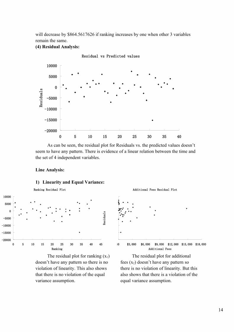
will decrease by $864.5617626 if ranking increases by one when other 3 variables remain the same.(4) Residual Analysis:
Residual vs Predicted values
-20000
-15000
-10000
-5000
0
5000
10000
0 5 10 15 20 25 30 35 40
Residuals
As can be seen, the residual plot for Residuals vs. the predicted values doesn’t seem to have any pattern. There is evidence of a linear relation between the time and the set of 4 independent variables.
Line Analysis:
1) Linearity and Equal Variance:
Ranking Residual Plot
-20000
-15000
-10000
-5000
0
5000
10000
0 5 10 15 20 25 30 35 40 45
Ranking
Residuals
The residual plot for ranking (x1) doesn’t have any pattern so there is no violation of linearity. This also shows that there is no violation of the equal variance assumption.
Additional Fees Residual Plot
-20000
-15000
-10000
-5000
0
5000
10000
$0 $3,000 $6,000 $9,000 $12,000 $15,000 $18,000
Additional Fees
Residuals
The residual plot for additional fees (x2) doesn’t have any pattern so there is no violation of linearity. But this also shows that there is a violation of the equal variance assumption.
14

Annual Cost Residual Plot
-20000
-15000
-10000
-5000
0
5000
10000
$0 $10,000 $20,000 $30,000 $40,000 $50,000
Annual Cost
Residuals
The residual plot for annual cost (x3) doesn’t have any pattern so there is no violation of linearity. This also shows that there is no violation of the equal variance assumption.
Placement success rank Residual Plot
-20000
-15000
-10000
-5000
0
5000
10000
0 10 20 30 40 50 60 70 80
Placement success rank
Residuals
The residual plot for placement success rank (x4) doesn’t have any pattern so there is no violation of linearity. This also shows that there is no violation of the equal variance assumption.
15
2) Normality:
Normal Probability Plot
-20000
-15000
-10000
-5000
0
5000
10000
-2.5 -2 -1.5 -1 -0.5 0 0.5 1 1.5 2 2.5
Z Value
Residuals
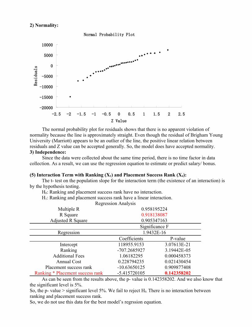
The normal probability plot for residuals shows that there is no apparent violation of normality because the line is approximately straight. Even though the residual of Brigham Young University (Marriott) appears to be an outlier of the line, the positive linear relation between residuals and Z value can be accepted generally. So, the model does have accepted normality.3) Independence:
Since the data were collected about the same time period, there is no time factor in data collection. As a result, we can use the regression equation to estimate or predict salary/ bonus.
(5) Interaction Term with Ranking (X1) and Placement Success Rank (X4):The t- test on the population slope for the interaction term (the existence of an interaction) is
by the hypothesis testing.H0: Ranking and placement success rank have no interaction.H1: Ranking and placement success rank have a linear interaction.
Regression AnalysisMultiple R 0.958195224R Square 0.918138087
Adjusted R Square 0.905347163Significance F
Regression 1.9432E-16Coefficients P-value
Intercept 118955.9153 3.07613E-21Ranking -707.2685927 3.19442E-05
Additional Fees 1.06182295 0.000458373Annual Cost 0.228794235 0.021430454
Placement success rank -10.63650125 0.909877408Ranking * Placement success rank -5.415720105 0.142358202
As can be seen from the results above, the p- value is 0.142358202. And we also know that the significant level is 5%.So, the p- value > significant level 5%. We fail to reject H0. There is no interaction between ranking and placement success rank.So, we do not use this data for the best model’s regrssion equation.

Math 240 Summer '10 Module #1
(6) The Best Model:So far we have produced the four multiple regression models with 4 variables (y = salary/
bonus, x1 = additional fees, x2 = annual cost, x3 = placement success rank, x4 = ranking):ŷ = b0 + b1 x1+ b2 x2+ b3 x3 + b4 x4
= 122190.0278 + 0.940489545 x1+ 0.220832356 x2
-133.6100862 x3 - 864.5617626 x4
with r = 0.955170424, r2 = 0.912350538, r2adj = 0.901726361.
Tough the r, r2, and r2adj of the t- test of the interaction term are a little higher than that of the
overall test, the best model is still the model used in the overall test because there is no interaction between ranking and placement success rank. We do not need to change the equation.
That is to say, the model (y = salary/ bonus, x1 = additional fees, x2 = annual cost, x3 = placement success rank, x4 = ranking) is the best model for us for estimating salary/ bonus.
Conclusions:The salary/ bonus are strongly related to additional fees, annual costs, placement success
rank, and ranking of MBA school. When a student wants to know how much salary/ bonus after he/ she graduates from a MBA school, he/ she need to consider these variables together. Because the 4 variables can help us explain 91.24% of the salary/ bonus of the overall MBA schools in our world. The multiple regression equation ŷ = 122190.0278 + 0.940489545 x1+ 0.220832356 x2
-133.6100862 x3 - 864.5617626 x4 (y = salary/ bonus, x1 = additional fees, x2 = annual cost, x3 = placement success rank, x4 = ranking) can be used to predicted or estimate the salary/bonus of MBA school.

Math 240 Summer '10 Module #1

Math 240 Summer '10 Module #1
[1] Answer the following true-false questions:
True or False
a) Only a normal distribution has a bell-shaped curve. False
b)The Student t distribution takes different values for a different sample
size.True
c)
The Central Limit Theorem states that if the original population is
normally distributed, the sample means will be normally distributed
for any sample size n (even if n < 30).
Ture
d)
According to the Central Limit Theorem, if the original population has
mean d = 30 and standard deviation r = 12, then the standard
deviation of the sample means of all possible random samples of size
36 is 1/3
False
e)
A 99% confidence interval is always better than a 95% confidence
interval because one can be more confident about the population
mean.
False
f)If s (population standard deviation) is not available, we can always
use s (sample standard deviation) to construct a confidence interval.False
g)A 95% confidence interval of 98.08 < r < 98.32 means that there is a
probability of 2.5% that the real will exceed 98.32.False
h)If the margin for sampling error is small, then the value of r must be
large.False
i)
According to the Chebyshev's rule, for any data set, regardless of
shape, 75 percentage of values can be found within distances of 2
standard deviations from the means.
False
j)The normal distribution has its interquartile range (IQR) equal to 1.33
standard deviations.Ture

Math 240 Summer '10 Module #1
[2](10) A small drugstore orders copies of a news magazine for its magazine rack each week.
Let x be the number of customers who come in to buy the magazine during a given week.
The probability distribution of x is
x 1 2 3 4 5 6
P(x) 1/15 2/15 3/15 4/15 3/15 2/15
The store pays $ .25 for each copy purchased, and the price of the magazine is $1.00. Any
magazines unsold at the end of the week have no value.
a) If the store orders three copies of the magazine, what is the mean value of the profit?
(Profit = Revenue – Cost)
Cost = 3 × $0.25 = $0.75
x 1 2 3 4 5 6Cost($) 0.75 0.75 0.75 0.75 0.75 0.75
Revenue($) 1 2 3 3 3 3Profit($) 0.25 1.25 2.25 2.25 2.25 2.25
P(x) 1/15 2/15 3/15 4/15 3/15 2/15So, E ( profit ) = $0.25 × 1/15 + $1.25 × 2/15 + $2.25 × 3/15 + $2.25 × 3/15 + $2.25 × 2/15
= $1.98
b) If the store orders four copies of the magazine, is it better to order four than three
copies of the magazine. Explain.
It is better to order four than three copies of the magazine.
Cost = 4 × $0.25 = $1.00
So, E ( profit ) = $0.00 × 1/15 + $1.00 × 2/15 + $2.00 × 3/15
+ $3.00 × 4/15 + $3.00 × 3/15 + $3.00 × 2/15
= $2.33
Then we can see the mean of profit for 4 copies is much higher than the mean of profit for 3
copies. This means ordering 4 copies of magazine is better than ordering 3 copies of magazine
because it can generate higher profit usually.
x 1 2 3 4 5 6Cost($) 1 1 1 1 1 1
Revenue($) 1 2 3 4 4 4Profit($) 0 1 2 3 3 3
P(x) 1/15 2/15 3/15 4/15 3/15 2/15

Math 240 Summer '10 Module #1
[3](10) Twenty-one percent of the executives in a large advertising firm are at the top salary level. It is
further known that 40 percent of all the executives at the firm are women. Also, 6.4 percent of all
executives are women and are at the top salary level. Recently, a question arose among executives at the
firm as to whether there is any evidence of salary inequality. Assuming that some statistical consideration
(explained in later chapters) are met, do the percentages reported above provide any evidence of salary
inequality? Substantiate your answer.
Top Salary Not Top Salary Total
Women 6.40% 33.60% 40%
Men 14.60% 45.40% 60%
Total 21% 79% 100%
Let event A = “women executives are at the top salary level”, and event B = “executives are at the
top salary level”.
So, P (A) = 40.00%, P (B) = 21.00%, P (A and B) = 6.40%
Then P (A) × P (B) = 40.00% × 21.00% = 8.40%,
P (A B) = (P (A∣ and B)) / P (B) = 6.40% / 21.00% = 30.48%,
As can be seen, P (A) × P (B) is not equal to P (A and B),
P (A B)∣ is not equal to P (A),
If P (A) × P (B) is equal to P (A and B), or P (A B)∣ is equal to P (A), event A and event B are
statistically independent, and there would be no salary inequality.
However, in this case, event A and event B are not statistically independent. That is to say, salary
inequality exists.

Math 240 Summer '10 Module #1
[4](10) Mars, Inc. claims that 14% of its M&M plain candies are yellow, and a sample of 100
such candies is randomly selected.
a) Find the mean and standard deviation for the number of yellow candies in such
groups of 100.
This is a binomial distribution because 100 trials have the same probabilities of yellow color or not
yellow color independently.
P (X) = 14%, n = 100
So, E (X) = n P (X) = 100 × 14% = 14
SD = {n P (X) [ 1 - P (X) ] }1/2 = ( 100 × 14% × 86% ) 1/2 = ( 12.04 ) 1/2 = 3.47
b) If a random sample of 100 M&Ms is selected, we find that there are only 8 yellow
candies in it. Is this result unusual? Does it seem that the claimed rate of 14% is
wrong? Explain.
n = 100, X real = 8, P (X) real = 8%
We know E (X) = 14, P (X) = 14%, SD = 3.47 from (a),
Based on this given information, the usual range “E (X) – 2 SD < X < E (X) + 2 SD” for 95%
of M&M in yellow color is “ 7.06 < X < 20.94 ”
And X = 8 is in this range.
As a result, this result is not unusual if the given information is correct.
n = 100 > 30, and we also know SD.
Because n P = 14 > = 5, n ( 1 – P) = 86 > = 5, we can use Z- distribution (normal distribution) to solve this case,
Normal ProbabilitiesCommon Data
Mean 14Standard Deviation 3.47
Probability for X <=X Value 8Z Value -1.729107
So, Z = ( X / n – P) / [ P ( 1 – P ) / n ] 1/2 = ( 8 / 100 – 14% ) / [14% ( 1 – 14%) / 100 ]1/2 = - 1.73
Then, the real SD = 1.73

Math 240 Summer '10 Module #1
So, the usual range “E (X) – 2 SD < X < E (X) + 2 SD” for 95% of M&M in yellow color is “ 10.54 < X < 17.46 ”.
Additionally, n P = 14 is in this range.
As a result, the claimed rate of 14% is right, and the result is not unusual.
[5](10) The lengths of pregnancies are normally distributed with a mean of 268 days and a
standard deviation of 15 days.
a) One classical use of the normal distribution is inspired by a letter to “Dear Abby” in
which a wife claimed to have given birth 308 days after a brief visit from her
husband, who was serving in the Navy. Given this information, find the probability of
pregnancy lasting 308 days or longer. What does the result suggest?
Mean = 268 days, SD = 15 days.
The usual range for 95% is “E (X) – 2 SD < X < E (X) + 2 SD”, which is “236 days < X <
298 days”.
So, usually, the pregnancy should be around 268 days, and 308 days for pregnancy is an unusual
event.
Additionally, we can use normal distribution to get its probability for at least 308 days:
Normal ProbabilitiesCommon Data
Mean 268Standard Deviation 15
Probability for X >X Value 308Z Value 2.6666667P(X>308) 0.0038
This means the probability of pregnancy lasting 308 days or longer is 0.38%.
It suggest that the probability of pregnancy lasting 308 days or longer is too small, and this event
almost could not happen.
As a result, there is a high possibility to support that the wife’s statement is wrong.
b) If we stipulate that a baby is premature if the length of pregnancy is in the lowest 4%,
find the length that separates premature babies from those who are not premature.
Premature babies often require special care, and this result could be helpful to
hospital administrators in panning for that care.
Normal ProbabilitiesCommon Data

Math 240 Summer '10 Module #1
Mean 268Standard Deviation 15
Find X and Z Given Cum. Pctage.Cumulative Percentage 4.00%Z Value -1.750686X Value 241.73971 So, the length that separates premature babies from those who are not premature is 242 days.
[6](10) A catering service has found that people eat an average of 7.4 ounces of shrimp at
affairs that it serves. The standard deviation is 2.4 ounces per person. The service is going
to cater an event for 100 people, and it plans to bring 50 pounds of shrimp. Determine that
probability that the caterer will run out of shrimp at the affair. (One pound = 16 ounces)
Population Mean = 7.4 ounces, Population SD = 2.4 ounces, n = 100 > 30,
So, according to the CLT,
The sampling distribution of the sample mean will be approximately normally distributed,
Sample Mean = Population Mean = 7.4 ounces,
Sample SD = Population SD / (Sample Size)1/2 = 2.4 ounces / (100)1/2 = 0.24 ounces,
Normal ProbabilitiesCommon Data
Mean 7.4Standard Deviation 0.24
Probability for X >X Value 8Z Value 2.5P(X>8) 0.0062096653 So, the probability that the caterer will run out of shrimp at the affair is 0.62%.

Math 240 Summer '10 Module #1
[7](10) A local law enforcement agency claims that the number of times that a patrol car passes through a particular neighborhood follows a Poisson process with a mean of three times per nightly shift.
a) Calculate the probability that no patrol car passes through the neighborhood during a nightly shift.
Because it is related to the number of person in certain period of time, we can treat it as a poisson
distribution.
Average occurrences over the same time period = 3
Poisson ProbabilitiesAverage/Expected number of successes: 3Poisson Probabilities Table
X P(X)0 0.049787
As a result, the probability that no patrol car passes through the neighborhood during a nightly
shift is 4.98%
b) Suppose that during a randomly selected night shift no patrol cars pass through the neighborhood. Based on your answer in a), would you believe the agency’s claim? Explain.
Yes. I would.X = 0, Population Mean = 3, P(X) = 4.98%, In posson distribution, SD = (Mean)1/2 = ( 3 ) 1/2 = 1.73So, the usual range “E (X) – 2 SD < X < E (X) + 2 SD” for 95% is “– 0.46 < X < 6.46”.
In reality, the usual range is adjusted, and it is “0 < = X < = 6”Tough the probability of X = 0 is very low, X = 0 could happen as a usual event because it is in the usual range.As a result, we can believe the agency’s claim.
c) Assuming that nightly shifts are independent and assuming that the agency’s claim is correct, find the probability that exactly one patrol car will pass through the neighborhood on each of four consecutive nights.
First of all, we need to get the probability that exactly one patrol car will pass through the
neighborhood on one night.
And the average occurrences over the same time period = 3
Poisson ProbabilitiesDataAverage/Expected number of successes: 3Poisson Probabilities Table
X P(X)1 0.149361
So, the probability that exactly one patrol car will pass through the neighborhood on one night is 14.94%.Due to the fact that the occurrences are independent, the probability that exactly one patrol car will pass through the neighborhood on each of four consecutive nights is (14.94%) 4 = 0.05%.
Math 240 Summer '10 Module #1
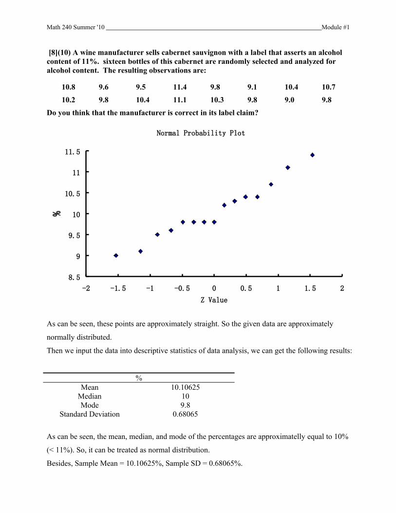
[8](10) A wine manufacturer sells cabernet sauvignon with a label that asserts an alcohol content of 11%. sixteen bottles of this cabernet are randomly selected and analyzed for alcohol content. The resulting observations are:
10.8 9.6 9.5 11.4 9.8 9.1 10.4 10.7
10.2 9.8 10.4 11.1 10.3 9.8 9.0 9.8
Do you think that the manufacturer is correct in its label claim?
Normal Probability Plot
8.5
9
9.5
10
10.5
11
11.5
-2 -1.5 -1 -0.5 0 0.5 1 1.5 2
Z Value
%
As can be seen, these points are approximately straight. So the given data are approximately
normally distributed.
Then we input the data into descriptive statistics of data analysis, we can get the following results:
%Mean 10.10625
Median 10Mode 9.8
Standard Deviation 0.68065
As can be seen, the mean, median, and mode of the percentages are approximatelly equal to 10%
(< 11%). So, it can be treated as normal distribution.
Besides, Sample Mean = 10.10625%, Sample SD = 0.68065%.

Math 240 Summer '10 Module #1
Because population SD is unknown and the given data is normally distributed, we use t
distribution to solve this problem.
Confidence Interval Estimate for the MeanData
Sample Standard Deviation 0.68065Sample Mean 10.10625Sample Size 16Confidence Level 95%
Intermediate CalculationsStandard Error of the Mean 0.1701625Degrees of Freedom 15t Value 2.131449536Interval Half Width 0.362692782
Confidence IntervalInterval Lower Limit 9.74Interval Upper Limit 10.47
So, the 95% confident interval is “9.74% < X < 10.47%”.
However, 11% is out of this range. So, it’s an unusual event.
As a result, the manufacturer is not correct in its label claim.

Math 240 Summer '10 Module #1
[9](10) A recent Gallup poll consisted of 1012 randomly selected adults who were asked whether “cloning of humans should or should not be allowed.” Results showed that 89% of those surveyed indicated that cloning should not be allowed.
a) Among the 1012 adults surveyed, how many said that cloning should not be allowed?
P (should not be allowed)= 89%
The number of respondents who said that cloning should not be allowed = 1012 × 89% = 900.68
So, 901 people said “cloning should not be allowed”
b) If we assume that people are indifferent so that 50% believe that cloning of humans
should not be allowed, find the mean and standard deviation for the numbers of
people in groups of 1012 that can be expected to believe that such cloning should not
be allowed.
Because of 1012 trials and fixed probabilities for the two outcomes, we can treat this as an
binomial distribution.
n = 1012, P = 50%.
So, Mean = n P = 1012 × 50% = 506
SD = [ n P ( 1 - P ) ] 1/ 2 = (1012 × 50% × 50%)1/2 = 15.91 (treated as 16 in reality)
Binomial ProbabilitiesData
Sample size 1012Probability of success 0.5
StatisticsMean 506Standard deviation 15.90597
As a result, the mean for the numbers of people in groups of 1012 that can be expected to believe
that such cloning should not be allowed is 506, and the standard deviation for the numbers of
people in groups of 1012 that can be expected to believe that such cloning should not be allowed is
16.

Math 240 Summer '10 Module #1
c) Based on the preceding results, does the 89% result for the Gallup poll appear to be
unusually higher than the assumed rate of 50%? Does it appear that an
overwhelming majority of adults believe that cloning of humans should not be
allowed?
Both of the answers are “Yes”.
Mean = 506,
SD = 16,
Then, the usual range “E (X) – 2 SD < X < E (X) + 2 SD” for 95% of M&M in yellow color is “474 < X < 538”.
However, if P = 89%, then X = 901 is out of this range.
As a result, the 89% result for the Gallup poll appear to be unusually higher than the assumed rate
of 50%.
E(X) = n P = n ( 1 - P ) = 506 > 5,
Then, Z = ( X / n – P) / [ P ( 1 – P ) / n ] 1/2
= ( 901 / 1012 – 50% ) / [50% ( 1 – 50%) / 1012 ]1/2 = 19.52
In reality, the real Z is 20, which is far away from the mean 506.
As a result, it appears that an overwhelming majority of adults believe that cloning of humans
should not be allowed because the result is beyond 2 times of SD from the mean.

Math 240 Summer '10 Module #1
[10](10) According to the U.S. Census Bureau, the mean household income in the United
States in 2000 was $57,045 and the median household income was $42,148 (U.S. Census
Bureau, “Money Income in the United States: 2000,” www.census.gov, September 2001).
The variability of household income is quite large, with the 90th percentile approximately
equal to $111,600, and an overall standard deviation of approximately $25,000. Suppose
random samples of 225 households were selected.
a) What proportion of the sample means would be below $55,000?
Population Mean = $57,045, Population Median = $42,148, Population SD = $25,000, n = 225 >
30,
So, according to the CLT,
The sampling distribution of the sample mean will be approximately normally distributed,
Sample Mean = Population Mean = $57,045,
Sample SD = Population SD / (Sample Size)1/2 = $25,000 / (225)1/2 = $1,666.6667,
Normal ProbabilitiesCommon Data
Mean 57045Standard Deviation 1666.6667
Probability for X <=X Value 55000Z Value -1.227P(X<=55000) 0.1099113
As a result, 10.99% of the sample means would be below $55,000.
b) What proportion of the sample means would be above $60,000?
Normal ProbabilitiesCommon Data
Mean 57045Standard Deviation 1666.6667
Probability for X >X Value 60000Z Value 1.773P(X>60000) 0.0381
As a result, 3.81%% of the sample means would be above $60,000.

Math 240 Summer '10 Module #1
c) What proportion of the sample means would be above $111,600?
Normal ProbabilitiesCommon Data
Mean 57045Standard Deviation 1666.666667
Probability for X >X Value 111600Z Value 32.733P(X>111600) 0.0000000
As a result, 0.00% of the sample means would be above $111,600.
d) Why is the probability you calculated in (c) so much lower than 0.10, even though 10%
of individual households have incomes above $111,600?
Population Mean = $57,045, Population SD = $25,000,
So, Population SD < Population Mean,
This means the distribution of the population is right- skewed.
However, the distribution of the sample is normal distribution.
So, the part of the right side of the sample distribution is much smaller than that of population
distribution.
As a result, the probability you calculated in (c) so much lower than 0.10, even though 10% of
individual households have incomes above $111,600.
e) If random samples of size 20 were selected, can you use the methods discussed in this
chapter to calculate the probabilities requested in (a)--(c)? Explain.
No.n = 20 < 30.So, it’s not the situation discripted in CLT, and it is not a normal distribution.According to the flow chart in hand out, we know that:When we don’t know the data is normally distributed, no matter SD is known or unknown, if n is not higher than 30 (n < = 30), the data should not be analyzed by normal distribution.As a result, there is no solution for this case.So we cannot use the methods discussed in this chapter to calculate the probabilities requested in (a)--(c).

Math 240 Summer '10 Module #1
(If I am the people who haven’t study CLT, I might use the method to deal with the problem. Unforturnately, I’m not that guy. Haha.) [1] Suppose that the following information is obtained from students upon exiting the campus bookstore during the first week of classes:
a) Amount of money spent on books
b) Number of textbooks purchased
c) Amount of time spent shopping in the bookstore
d) Academic major
e) Gender
f) Ownership of a laptop computer
g) Ownership of an MP3 player
h) Number of units registered for in the current semester
i) Whether or not any clothing items were purchased at the bookstore
j) Method of payment
Classify each of the measurements as nominal, ordinal, interval, ratio scales, discrete or continuous.
qualitative quantitative
nominal ordinal interval ratio discrete continuousa) Yes Yesb) Yes Yesc) Yes Yesd) Yese) Yesf) Yesg) Yesh) Yes Yesi) Yesj) Yes
In general, is the measurement “amount of money spent on something” a continuous or discrete variable? Discuss it briefly in your own words.
According to the text book, discrete variable can be an integer of a counting process, while continuous variable can be both an integer and a continuum of a measuring process by measuring instruments with different precision.
In this case, the amount of money spent on something can only be an integer that can be counted. For instance, peple count money as intergers because we don’t have cash that has countless number. So it doesn’t have relationship with a measuring process. Therefore, I regard “amount of money spent on something” is a discrete variable.

Math 240 Summer '10 Module #1
[2] The director of market research at a large department store chain wanted to conduct a survey throughout a metropolitan area to determine the amount of time working women spend shopping for clothing in a typical month.
a) Describe both the population and the sample of interest, and indicate the type of data the director might want to collect.
1) In this survey, the population of interest is all the working women throughout the metropolitan, and the sample of interest is some of those working women that are chosen to participate in the survey. The sample is part of the population.
2) The director of market research wanted to use the data for his analysis, so he is the data collector. In other words, the data comes from primary sources. In addition, because the director wanted to conduct the survey, the data can be identified as a survey from primary sources. In the survey, the director can ask questions about beliefs, attitudes, behaviors, and other characteristics of respondents.
b) Develop a first draft of the questionnaire needed in (a) by writing a series of three categorical questions and three numerical questions that you feel would be appropriate for this survey.
1) 3 categorical questions:
(1) Do you think you are rich?
Yes/No
(2) Do you care more about your dressing than other working women?
Yes/No
(3) What type of body shape do you have?
A. Fat;
B. Normal;
C. Thin
2) 3 numerical questions:
(1) How many clothes do you try in each clothes shop?
A. 0;
B. 1 or 2;
C. 3-5;
D. more than 5
(2) What’s the highest price of one clothing you can afford?
A. Less than $50;
B. $50- $100;
C. $100- $200;
D. More than $200
(3) How much time do you spend on considering buying one clothing?
A. In 1 min;
B. 2min- 5min;
C. 5min-15min;
D. More the 15min

Math 240 Summer '10 Module #1
[3] America Online posted this question on its Web site: “How much stock do you put in long-range weather forecasts?” Among its Web site users, 38,410 chose to respond.
a) Among the responses received, 5% answered with “a lot.” What is the actual number of responses consisting of “a lot?”
1921
b) Among the responses received, 18,053 consisted of “very little or none.” What percentage of responses consisting of “very little or none?”
47%
c) Because the sample size of 38,410 is so large, can we conclude that about 5% of the general population puts “a lot” o stock in long-range weather forecasts? Why or why not?
No.
The big size of sample size donesn’t mean that it represents the general population because the sample is only part of the general population.
The best way to estimate the general population is to select large number of sample size radomly and then analysz them. If almost all of the results of the sample size have similar estimation, then the sample size can tell us the most creditable estimation about the general population.
However, in this case, it has only one estimation by getting one sample size. Different results still might appear if we selesct another big sample size and estimate it.
As a result, we cannot conclude that about 5% of the general population puts “a lot” o stock in long-range weather forecasts based on the big sample size.
[1] In an article in the November 1993 issue of Quality Progress, Barbara A. Cleary reports on improvements made in a software supplier’s responses to customer calls. In this article, the author states:
In an effort to improve its response time for these important customer-support-calls, an inbound telephone inquiry team was formed at PQ Systems, Inc., a software and training organization in Dayton, Ohio. The team found that 88 percent of the customers’ calls were already being answered immediate by the technical support group, but those who had to be called back had to wait an average of 56.6 minutes. No customer complaints had been registered, but the team believed that this response rate could be improved.
As part of its improvement process, the company studied the disposition of complete and incomplete calls to its technical support analysis. A call is considered complete if the customer’s problem has been resolved; otherwise the call is incomplete. Below is the summary table for the incomplete customer calls.
Action by Technical Support Analysts PercentageRequired customer to get more data 29.17Required more investigation by us 28.12Callbacks 21.87Required development assistance 12.50Required administrative help 4.17Determined as actually a new problem 4.17

Math 240 Summer '10 Module #1
a) Construct a Pareto chart

Math 240 Summer '10 Module #1
The Pareto Diagram for Technical Support Analysts
0.00%
5.00%
10.00%
15.00%
20.00%
25.00%
30.00%
35.00%R
equi
red
cust
omer
to g
et m
ore
data
Req
uire
d m
ore
inve
stig
atio
n by
us
Cal
lbac
ks
Req
uire
d de
velo
pmen
t ass
istan
ceR
equi
red
adm
inist
rativ
e he
lp
Det
erm
ined
as a
ctua
lly a
new
pro
blem
Actions
0.00%
10.00%
20.00%
30.00%
40.00%
50.00%
60.00%
70.00%
80.00%
90.00%
100.00%
b) What percentage of incomplete calls required “more investigation” by the analyst or “administrative
help?”
According to the given information, 28.12%of incomplete calls required “more investigation” by the
analyst, and 4.17% of incomplete calls required “administrative help”. As a result, the percentage of
incomplete calls required “more investigation” by the analyst or “administrative help” is the sum of the
persentages of “more investigation” and “administrative help”, which is : 28.12% + 4.17% = 32.29%.
c) Can you make a suggestion to improve responses?
The majority of incomplete calls required “more data” from customer and “more investigation” by the analyst. So, communication between analyst and customers can solve the problem efficiently.

Math 240 Summer '10 Module #1
[2] Do the problem 3.35 on p.126. This problem is intended for you to learn EDA (Exploratory Data Analysis).
a))
Five-number Summary for the Yield of the Money Market Account, One-Year CD, and a Five-Year CD
Money Market Account One-Year CD Five-Year CD
Minimum 0.1 1.55 3.15
First Quartile 0.5 3.05 3.9
Median 0.65 3.525 4.09
Third Quartile 1.01 4 4.35
Maximum 2.27 4.6 5.12
b)
Box-and-Whisker Plot for the Yield of the Money Market Account, One- Year CD, a Five- Year CD.
Money Market
One-Year CD
Five-Year CD
0 1 2 3 4 5 6
c) Both of the distribution of the money market account and the five-year CD are right-skewed, and the distribution of the one-year CD is left-skewed. But the distribution of the five- year CD is closed to a bell- shaped distribution.

Math 240 Summer '10 Module #1
Money market: Minimum = 0.1. Maximum = 2.27
Q1 – (IQR × 1.5) = Q1 – [(Q3 – Q1) × 1.5] = 0.5 – [ ( 1.01 – 0.5) × 1.5] = -0.265 Q3 + (IQR × 1.5) = Q3 + [(Q3 – Q1) × 1.5] = 1.01 + [ ( 1.01 – 0.5) × 1.5] = 1.775 So, Q1 – (IQR × 1.5) < the minimum < Q3 + (IQR × 1.5) < the maximumAs a result, the maximum value 2.27 is an outlier.
One-year CD:Minimum = 1.55
Maximum = 4.6Q1 – (IQR × 1.5) = Q1 – [(Q3 – Q1) × 1.5] = 3.05 – [ ( 4 – 3.05) × 1.5] = 1.625Q3 + (IQR × 1.5) = Q3 + [(Q3 – Q1) × 1.5] = 4 + [ ( 4 – 3.05) × 1.5] = 5.425 So, the minimum < Q1 – (IQR × 1.5) < the maximum < Q3 + (IQR × 1.5) As a result, the minimum value 1.55 is an outlier.
Five-year CD:Minimum = 3.15
Maximum = 5.12Q1 – (IQR × 1.5) = Q1 – [(Q3 – Q1) × 1.5] = 3.9 – [ ( 4.35 – 3.9) × 1.5] = 3.225Q3 + (IQR × 1.5) = Q3 + [(Q3 – Q1) × 1.5] = 4.35 + [ ( 4.35 – 3.9) × 1.5] = 5.025So, the minimum < Q1 – (IQR × 1.5) < Q3 + (IQR × 1.5) < the maximumAs a result, the minimum value 3.15 and the maximum value 5.12 are outliers.
Mean Standard Deviation Coefficient of Variation
Money Market 0.8165 0.521194634 63.83%
One-Year CD 3.53675 0.677621737 19.16%
Five-Year CD 4.13475 0.390745425 9.45%
Because the coefficient of variation of the money market is the highest one, the yield of the monet market is the most variable data in the group. Then the yield of the one- year CD is less variable, and the yield of the five- year CD is the lease variable data.
Math 240 Summer '10 Module #1
[3] Maximum breadth of sample of male Egyptian skulls from 4000 B.C. and 150 A.D. (based on data from
Ancient Races of the Thebaid by Thompson and Randall-Maciver):
4000 B.C. 131 119 138 125 129 126 131 132 126 128 128 131150 A.D. 136 130 126 126 139 141 137 138 133 131 134 129
a) Find the mean, median, and mode, range, variance, and the standard deviation for each of the two samples.
4000 B.C. 150 A.D.
Mean 128.6666667 133.3333333
Median 128.5 133.5
Mode 131 126
Range 19 15
Variance 21.51515152 25.15151515
Standard Deviation 4.63844279 5.015128628
b) Compare and analyze the two data sets using descriptive measures.
Based on the data of (a), we know that:
For 4000 B.C. : Mean = E (X) = 128.6666667 (almost the same as Median),
SD = 4.63844279,
So, the “usual range” E (X) – 2 SD < X < E (X) + 2 SD is 119.39 < X < 137.95.
Only 138 and 139 is out of this range. Other datas are within this “usual range”.
For 150 A.D. : Mean = 133.3333333(almost the same as Median),
SD = 5.015128628,
So, the “usual range” E (X) – 2 SD < X < E (X) + 2 SD is 123.29 < X < 143.37.
All the datas are within this “usual range”.

Math 240 Summer '10 Module #1
c) Changes in head size over time suggest interbreeding with people from other regions. Do the head sizes appear to have changed from 4000 B.C. to 150 A. D.? Explain.
Yes.
Box-and-Whisker Plot
4000 B.C.
150 A.D.
110 120 130 140 150
As can be seen, the smallest size, the Q1, the mean size, the Q3, and the largest size of people of 150 A.D. were larger than that of people of 4000 B.C. repectively. The interbreeding with people from different areas cause different combination of gene from different race. Additionally, some gene determines the breadth of sample of male Egyptian skulls. Over a period of time, from 4000 B.C. to 150 A. D., the maximum breadth of sample of male Egyptian skulls change because their gene mixed with that of other regions.

Math 240 Summer '10 Module #1
[4] In an article in the Journal of Marketing, pp.22-37, (January 1992), Mazis, Ringold, Perry, and Denman discuss the perceived ages of models in cigarette advertisements. To quote the authors:
Most relevant to our study is the Cigarette Advertiser's Code, initiated by the tobacco industry in 1964. The code contains nine advertising principles related to young people, including the following provision (Advertising Age 1964): “Natural persons depicted as smokers in cigarette advertising shall be at least 25 years of age and shall not be dressed or otherwise made to appear to be less than 25 years of age.”
Tobacco industry representatives have steadfastly maintained that code provisions are still being observed. A 1988 Tobacco Institute Publication, “Three Decades of Initiatives by a Responsible Cigarette Industry, “refers to the industry code as prohibiting advertising and promotion “directed as young people” and as “requiring that models in advertising must be, and must appear to be, at least 25 years old.” John R. Nelson, Vice President of Corporate Affairs for Philip Morris, recently wrote, “We employ only adult models in our advertising that not only are but look over 25” (Nelson 1990). However, industry critics have charged that current cigarette advertising campaigns use unusually young-looking models, thereby violating the voluntary code.
Now suppose that a sample of 50 people is randomly selected at a shopping mall. Each person in the sample is shown a typical cigarette advertisement and is asked to estimate the age of the model in the ad. Below is the 50 perceived ages so obtained. The data set (tobacco.xls) is downloadable at Doc Sharing.
24 28 24 26 29 27 28 18 28 2123 28 25 30 22 29 20 27 24 2329 22 27 17 20 27 21 29 26 2826 27 23 27 27 30 28 19 25 2922 24 24 30 27 25 26 28 20 24
a) Construct a relative frequency (percentage) histogram and a cumulative percentage polygon (ogive) for the 50 perceived ages.
Histogram for Tobacco Industry
0%
5%
10%
15%
20%
25%
30%
35%
19 21 23 25 27 29 31
Ages
Freqyency

Math 240 Summer '10 Module #1
Cumulative Percentage Polygon for Tobacco Industry
0%
10%
20%
30%
40%
50%
60%
70%
80%
90%
100%
19 21 23 25 27 29
b) What percentage of the perceived ages is below the industry's code provision (of 25 years old)? Do you think that this percentage is too high?
40% of the perceived ages are below the industry’s code provision (of 25 years old). In my opinion, this percentage is too high.
[1] A sample of 500 respondents was selected in a large metropolitan area to determine various information concerning consumer behaviors. Among the questions asked was “Do you enjoy shopping for clothing?” Of 240 males, 136 answered yes. Of 260 females, 224 answered yes.
a) Is “enjoy shopping for clothing” gender-independent? Explain.
No.
Number of RespondentsAnswers
Yes NoTotal
GenderMales 136 104 240
Females 224 36 260
Total 360 140 500 P ( enjoy ) = 360 / 500 =72% P ( male ) = 240 / 500 = 48% P ( enjoy and male ) = 136 / 500 = 27.2%

Math 240 Summer '10 Module #1
So, P ( enjoy ) P ( male ) = 72% × 48% = 34.56%,P ( enjoy | male ) = P ( enjoy and male ) / P ( male ) = 27.2% / 48% = 56.67%,
As a result, P ( enjoy ) P ( male ) is not equal to P ( enjoy and male ); P ( enjoy | male ) is not equal to P ( enjoy ), If P ( enjoy ) P ( male ) is equal to P ( enjoy and male ); P ( enjoy | male ) is equal to P ( enjoy ), then event “enjoy shopping for clothing” is gender- independent. However, in this case, the equation above cannot be achieved. So, “enjoy shopping for clothing” is not gender-independent
b) Are “enjoy shopping for clothing” and “being a male” mutually exclusive? Explain.
No.
If “enjoy shopping for clothing” and “being a male” are mutually exclusive, then P ( enjoy and male ) is equal to nothing.
However, in this case, we know “P ( enjoy and male ) = 136 / 500 = 27.2%” from (a). So, P ( enjoy and male ) is not equal to nothing. As a result of this, “enjoy shopping for clothing” and “being a male” are not mutually exclusive.
c) What is the probability that a respondent chosen at random is a male if the person answered no?
Event A: a respondent is a male
Event B: the answer of a respondent is no So, P (A) = number of males/ number of all respondents = 240/ 500 = 48%
P (B) = number of people who answered no/ number of all respondents = [(240- 136) + (260- 224)]/ 500 = (104+ 36)/ 500 = 140/ 500 = 28%
As we can seen in the chart above, P (A and B) = 104/ 500 = 20.8%Due to the face that answering no happened first as a condition, we treat this situation as
conditional probability.As a result, given the condition that the person answered no, the probability for “a
respondent chosen at random is a male” is:P (A| B) = P (A and B)/ P (B) = 20.8%/ 28% = 74.29%

Math 240 Summer '10 Module #1
[2] The sport director of a local television station surveyed a random sample of 100 viewers on their preferences regarding coverage of certain events. The survey revealed that 70 preferred coverage of San Francisco Giants' game, 26 preferred coverage of WNBA, and 6 preferred both. One of the viewers is selected at random. Find the following probabilities.
a) The viewer preferred coverage of Giants' games.
OpinionsGaints
Yes NoTotal
WNBAYes 6 20 26
No 64 10 74
Total 70 30 100In this case, assume that event A is “70 viewers preferred coverage of SF Gaint’s game”,
event B is “26 viewers preferred coverage of WNBA”.
The probability of event A is: P (A) = 70/ 100 = 70%
b) The viewer preferred at least one of coverages.
P (B) = 26/100 = 26%
P (A and B) = 6/100 = 6%
Because event A and B can happen at the same time, they are not mutually exclusive.
So, P (A or B) = P (A) + P (B) - P (A and B) = 70% + 26% - 6% = 90%
c) The viewer preferred coverage of neither event.
P (not A and not B) = 1 - P (A or B) = 1- 90% = 10%
d) The viewer preferred coverage of WNBA if he/she has already preferred coverage of Giants' games
This is a conditional probability, and the condition is event A.
As we can seen in the chart above,
P (A and B) =6/ 100 = 6%
As a result, P (B| A) = P (A and B) / P (A) = 6% / 70% = 8.57%

Math 240 Summer '10 Module #1
[3] Two baseball teams, the San Francisco Giants and the Los Angeles Dodgers, will play each other for the league championship. The Giants are, in fact the better team. (But the Dodgers have the better yell, “That's all right, that's okay. You'll be working for us someday.”) According to Brett Mullin as of April 18, 2010, the Giants have won 1162 games and the Dodgers have won 1143 games since October 18, 1889, including their days while in New York.
a) What is the probability that the Giants will win the championship if these two teams play just one game?
Assume that event A is “the Giants will win the championship”,
event B is “the Dodgers will win the championship”,
So, P (A) = 1162 / (1162+ 1143) = 1162/ 2305= 50.41%
b) What is the probability that the Giants will win the championship if these two teams play a 5-game series?
If they play a 5-game series and the Gaints will win, the number of victories for the Giants must larger than the Dodgers’. The outcomes are as follows:
(1) A happens 3 times: P ( 1 ) = [ P ( A ) ] 3
(2) A happens 3 times, while B happens 1 time: P ( 2 ) = 3 × [ P ( A ) ] 3 × P ( not A )
(3) A happens 3 times while B happens 2 times: P ( 3 ) = 6 × [ P ( A ) ] 3 × [ P ( not A ) ] 2
Because the 3 situation above are mutually exclusive,
P [ ( 1 ) or ( 2 ) or ( 3 ) ] = P ( 1 ) + P ( 2 ) + P ( 3 )
= [ P ( A ) ] 3 + 3 × [ P ( A ) ] 3 × P ( not A ) + 6 × [ P ( A ) ] 3 × [ P ( not A ) ] 2
= [ P ( A ) ] 3 + 3 × [ P ( A ) ] 3 × [ 1 - P ( A ) ] + 6 × [ P ( A ) ] 3 × [ 1 - P ( A ) ] 2
= (50.41% ) 3 + 3 ×(50.41% ) 3 × ( 1 - 50.41% ) + 6 × (50.41% ) 3 × ( 1 - 50.41% ) 2
= 50.77%
As a consequence, the probability that the Giants will win the championship if these two teams play a 5-game series is 50.77%.

Math 240 Summer '10 Module #1
[4] At a certain gas station, 40% of all customers fill their tanks. Of those who fill their tanks, 80% pay with a credit card.
a) What is the probability that a randomly selected customer fills his or her tank and pays with a credit card?
Assume that event A is “the customer fills his or her tank”, and event B is “the customer pays with a credit card”.
This is a conditional probability because the customer pay with a credit card after he or her has filled his or her tank.
So, P (A) = 40%.
P (B| A) = 80%
As a result, P (A and B) = P (B| A) × P (A) = 80% × 40% = 32%
b) If three customers are randomly selected, what is the probability that all three fill their tanks and pay with a credit card?
Due to the face that the selections happened at the same time, they are independent events.
As a result, the probability that all three fill their tanks and pay with a credit card is:
[P ( A and B ) ] 3 = ( 32% ) 3 = 3.28%

Math 240 Summer '10 Module #1
[5] The probability is 0.70 that a rare tropical disease will be treated correctly. If it is treated correctly, the probability that the patient will be cured is 0.90. If it is not treated correctly, the probability is only 0.40 that the patient will be cured.
a) What is the probability that a randomly selected patient having this disease will be cured?
Assume that event A is “the disease will be treated correctly”, event B is “the disease will be cured”.
P (A) = 70%
P (not A) = 30%
P (B| A) = 90%
P (B| not A) = 40%
According to decision tree,
(1) P (A) = 70%: P (A and B) =P (B| A) × P (A) = 90% × 70% = 63%
P (A and not B) =P (not B| A) × P (A) = [1- P (B| A)] ×P (A)
= (1- 90%) × 70% = 10% × 70% = 7%
(2) P (not A) = 30%: P (not A and B) =P (B| not A) × P (not A) = 40% × 30% = 12%
P (not A and not B) =P (not B| notA) × P (not A)
= [1- P (B| notA)] ×P (not A) = (1- 40%) × 30%
=60% × 30% = 18%
The the disease will be cured under two situation, one is “the disease is treated correctly”, another one is “the disease is not treated correctly”.
P (A and B) or P (not A and B) cannot happen at the same time. So, they are mutually exclusive.
As a result, P (B) = P (A and B) + P (not A and B) = 63% + 12% = 75%
b) Suppose that a randomly selected patient having this disease is cured, what is the probability that it was not treated correctly?
Because P(not A and B) = P(B) ×P(not A| B) = P(not A) × P(B| not A),
We can get:
P (not A| B) = P (not A) and B) / P (B) = 12%/ 75% = 16
[1] In a clinical trial of Lipitor, a common drug used to lower cholesterol, 863 patients were given a treatment of 10-mg Atorvastatin tablets. Among them, 19 patients experienced flu symptoms and 844 patients did not (based on data from Pfizer, Inc.).
a) Estimate the probability that a patient taking the drug will experience flu symptoms.
The average occurences is 19 / 863 = 2.2%
We use possion distribution.
Poisson ProbabilitiesData

Math 240 Summer '10 Module #1
Average/Expected number of successes: 0.022Poisson Probabilities Table
X P(X)1 0.021521
As a result, the probability that a patient taking the drug will experience flu symptoms is 2.15%.
b) Is this unusual for a patient taking the drug to experience flu symptoms? Explain.
It is unusual.
Mean = 0.022 = SD2
So SD = 0.15
The the “usual range” E (X) – 2 SD < X < E (X) + 2 SD is - 0.28 < X < 0.32.
However, X = 1 is out of the usual range.
As a result, it is unusual for a patient taking the drug to experience flu symptoms.
c) If you know that the probability of flu symptoms for a person not receiving any treatment is 0.019, what is the probability that there are 19 who experience flu symptoms among 863 patients? Explain.
863 people are independent.
Two outcomes are “experience flu symptomes” and “ not experience flu symptomes”
P (experience flu symptomes) = 1.9% is fixed.
So, it’s a binomial distribution.
Binomial ProbabilitiesData
Sample size 863Probability of success 0.019Binomial Probabilities Table
X P(X)19 0.075404
So, P (X = 19) = 8.54%
The probability that there are 19 who experience flu symptoms among 863 patients is 7.54%
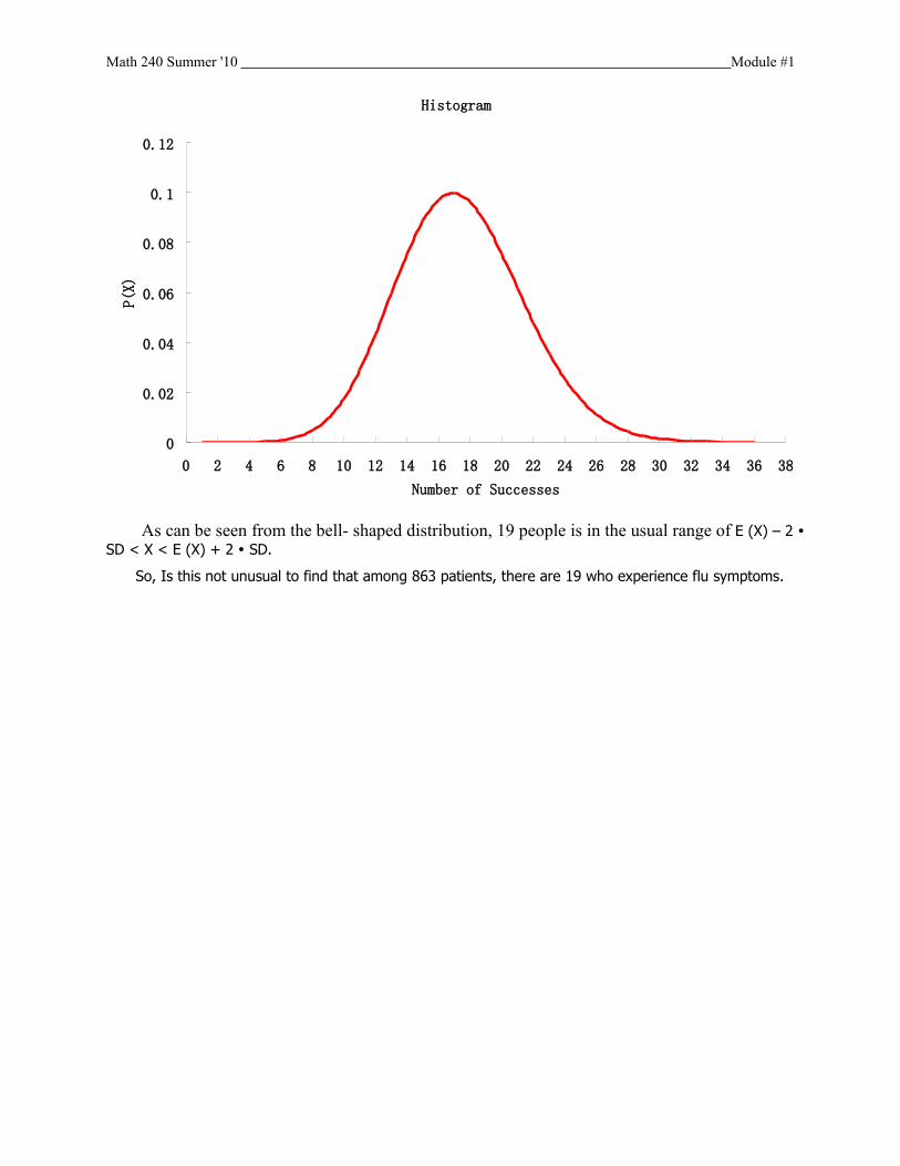
d) Is this unusual to find that among 863 patients, there are 19 who experience flu symptoms in c)? Explain.
Math 240 Summer '10 Module #1
Histogram
0
0.02
0.04
0.06
0.08
0.1
0.12
0 2 4 6 8 10 12 14 16 18 20 22 24 26 28 30 32 34 36 38
Number of Successes
P(X)
As can be seen from the bell- shaped distribution, 19 people is in the usual range of E (X) – 2 SD < X < E (X) + 2 SD.
So, Is this not unusual to find that among 863 patients, there are 19 who experience flu symptoms.
Math 240 Summer '10 Module #1
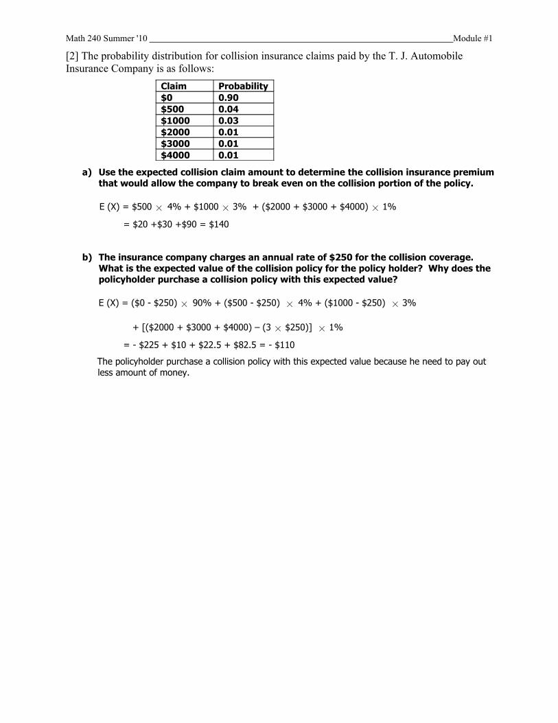
[2] The probability distribution for collision insurance claims paid by the T. J. Automobile Insurance Company is as follows:
Claim Probability$0 0.90$500 0.04$1000 0.03$2000 0.01$3000 0.01$4000 0.01
a) Use the expected collision claim amount to determine the collision insurance premium that would allow the company to break even on the collision portion of the policy.
E (X) = $500 × 4% + $1000 × 3% + ($2000 + $3000 + $4000) × 1%
= $20 +$30 +$90 = $140
b) The insurance company charges an annual rate of $250 for the collision coverage. What is the expected value of the collision policy for the policy holder? Why does the policyholder purchase a collision policy with this expected value?
E (X) = ($0 - $250) × 90% + ($500 - $250) × 4% + ($1000 - $250) × 3%
+ [($2000 + $3000 + $4000) – (3 × $250)] × 1%
= - $225 + $10 + $22.5 + $82.5 = - $110
The policyholder purchase a collision policy with this expected value because he need to pay out less amount of money.

Math 240 Summer '10 Module #1
[3] On average, 70 percent of the passengers on a flight from San Francisco to Boston prefer chicken to fish. Assume that the passengers have only one of two choices, chicken or fish for their meal. If there are 200 passengers on a flight and the airline carries 140 chickens and 60 fish dinners, what is the probability that more than three passengers won’t get what they wish for?
(1) This is Hypergeometric Distribution.
200 passengers mamake the same decision, so n = 200.
Each decision has 2 outcomes, chicken or fish
The probability of choosing chicken or fish is fixed.
Each people make their decision individually, so 200 trials are all independent.
As a result, this is a binomial distribution.
“More than three passengers who want chicken won’t get chicken” means more than 3 people who want chicken will get fish, and more than 3 people who want fish will get chicken.
Then we choose “137 < X < 143” as an object range. (140 – 3 = 137, 140 + 3 = 143)
Assume “success” is “get fish”, “failure” is “get chicken”
Then, P ( more than 3 people get fish) = 1 – P ( > = 3 people get fish)
P (success) = 140 / (140 + 60 ) = 70%
Binomial ProbabilitiesData
Sample size 200Probability of success 0.7Binomial Probabilities Table
X P(X) P(<=X) P(<X) P(>X) P(>=X)137 0.05453 0.346651 0.292121 0.653349 0.707879138 0.058086 0.404737 0.346651 0.595263 0.653349139 0.060454 0.465191 0.404737 0.534809 0.595263140 0.061462 0.526653 0.465191 0.473347 0.534809141 0.061026 0.587678 0.526653 0.412322 0.473347142 0.059164 0.646842 0.587678 0.353158 0.412322143 0.055992 0.702833 0.646842 0.297167 0.353158
So, P ( X < 137) = 0.292121,
P ( X > 143) = 0.297167
As a result, P (More than three passengers who want chicken won’t get chicken)
= P ( X < 137) + P ( X > 143) = 0.292121 + 0.297167 = 0.589288 = 58.93%
Math 240 Summer '10 Module #1
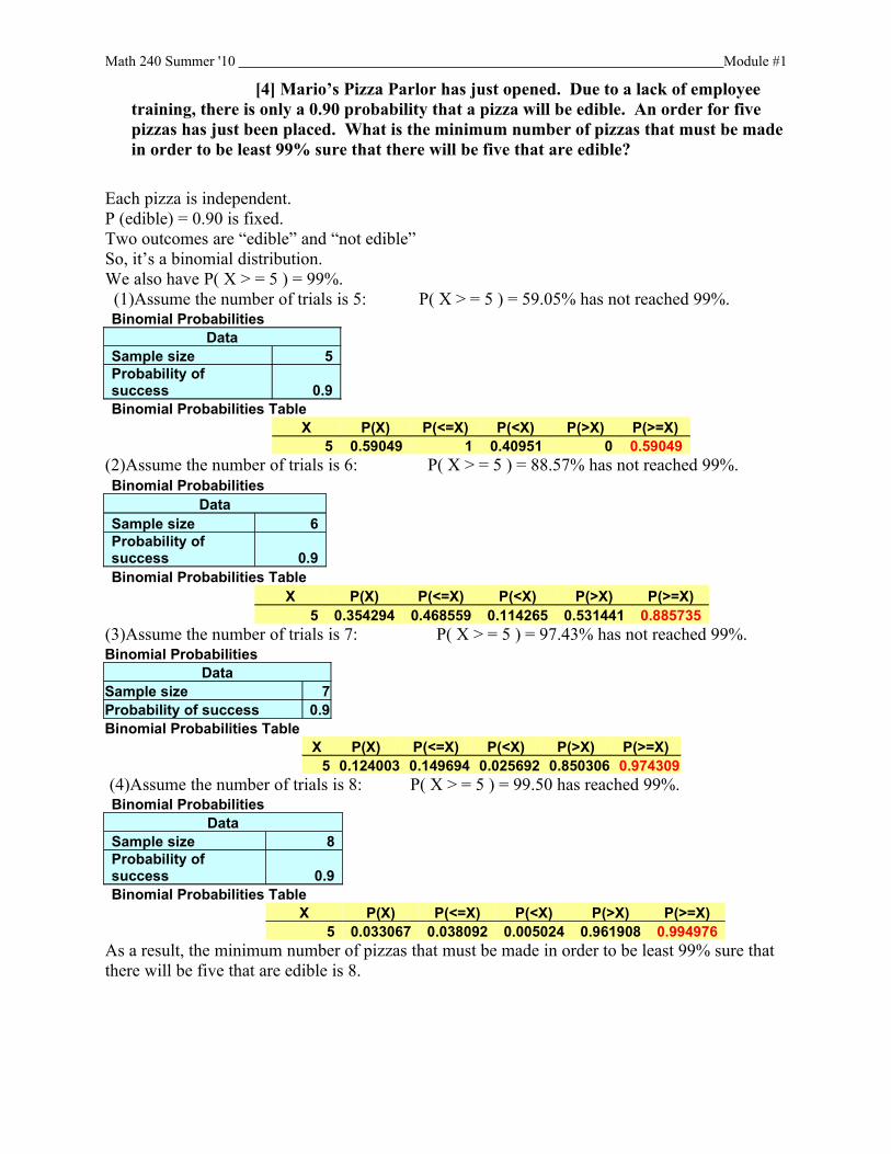
[4] Mario’s Pizza Parlor has just opened. Due to a lack of employee training, there is only a 0.90 probability that a pizza will be edible. An order for five pizzas has just been placed. What is the minimum number of pizzas that must be made in order to be least 99% sure that there will be five that are edible?
Each pizza is independent. P (edible) = 0.90 is fixed.Two outcomes are “edible” and “not edible”So, it’s a binomial distribution.We also have P( X > = 5 ) = 99%.(1)Assume the number of trials is 5: P( X > = 5 ) = 59.05% has not reached 99%. Binomial Probabilities
DataSample size 5Probability of success 0.9Binomial Probabilities Table
X P(X) P(<=X) P(<X) P(>X) P(>=X)5 0.59049 1 0.40951 0 0.59049
(2)Assume the number of trials is 6: P( X > = 5 ) = 88.57% has not reached 99%. Binomial Probabilities
DataSample size 6Probability of success 0.9Binomial Probabilities Table
X P(X) P(<=X) P(<X) P(>X) P(>=X)5 0.354294 0.468559 0.114265 0.531441 0.885735
(3)Assume the number of trials is 7: P( X > = 5 ) = 97.43% has not reached 99%. Binomial Probabilities
DataSample size 7Probability of success 0.9Binomial Probabilities Table
X P(X) P(<=X) P(<X) P(>X) P(>=X)5 0.124003 0.149694 0.025692 0.850306 0.974309
(4)Assume the number of trials is 8: P( X > = 5 ) = 99.50 has reached 99%. Binomial Probabilities
DataSample size 8Probability of success 0.9Binomial Probabilities Table
X P(X) P(<=X) P(<X) P(>X) P(>=X)5 0.033067 0.038092 0.005024 0.961908 0.994976
As a result, the minimum number of pizzas that must be made in order to be least 99% sure that there will be five that are edible is 8.

Math 240 Summer '10 Module #1
[5] You are the owner of a small lawn and garden service in Minneapolis. You are going to buy a new snow thrower and wish to assess the chance of receiving a complete purchase price rebate from the Taro Company. Taro's advertisements state that the company will refund the entire price of a machine if this winter's snow fall is less than 20% of the local average snowfall. The weather service reports that the average snowfall in your area is 46.0 inches, with the standard deviation of 15.2 inches based on the normal distribution. How likely is it that this rebate will happen?
Mean = E (X) = 46.0Standard Deviation = 15.220% of the local average snowfall = 20% × 46 = 9.2 inchesNormal Probabilities
Common DataMean 46Standard Deviation 15.2
Probability for X <=X Value 9.2Z Value -2.421053P(X<=9.2) 0.0077378Because SD 2 = Z 2, SD = 2.421053So the usual range “E (X) – 2 SD < X < E (X) + 2 SD” for snowfall is “41.157894 < X < 50.842106”
However, 9.2 inches is not in this range, so this rebate will not happen.
[1] A soft-drink manufacturer claims that its 12-ounce cans do not contain, on average, more than 30 calories. A random sample of 16 cans of this soft drink, which were checked for calories, contained a mean of 31.8 calories with a standard deviation of 3 calories. Assume that the number of calories in 12-ounce soda cans is normally distributed.
a) State the null and alternative hypotheses.
The null hypotheses is : 12-ounce cans do not contain more than 30 calories on average
( H0: Population Mean < = 30 calories)
The alternative hypotheses is : 12-ounce cans contain more than 30 calories on average
( H1: Population Mean > 30 calories)
b) Select the distribution to use. Explain briefly why you selected it.
I select t- distribution.
We know that the population distribution is normal distribution, so the sample population is also normally distributed.
n = 16 < 30, Sample Mean = 31.8 calories, Sample SD = 3 calories, and the population SD is unknown.
As a result, knowing “the sample is normally distributed” and “population SD is unknown”, we use t- distribution.
c) Assuming that they wish to test the claim at α = 0.025, determine the rejection and non rejection regions based on your hypotheses in a). State the critical value.

Math 240 Summer '10 Module #1
Significance level = 0.025,
This is an upper‐tail test. According to the t‐table on page 794 of the text book, the critical value for the 2.5% significance level with the degrees of freedom 15 (= 16-1) is 2.1315.
d) Calculate the value of the test statistic.
Population Mean = 30 calories,
n = 16, Sample Mean = 31.8 calories, Sample SD = 3 calories,
So, t = ( Sample Mean – Population Mean ) / [ Sample SD / ( n ) 1/2 ] = ( 31.8 – 30) / [3 / (16 ) 1/2 ]
= 1.8 / (3/4) = 2.4
t Test for Hypothesis of the MeanData
Null Hypothesis µ= 30Level of Significance 0.025Sample Size 16Sample Mean 31.8Sample Standard Deviation 3
Intermediate CalculationsStandard Error of the Mean 0.75Degrees of Freedom 15t Test Statistic 2.4
Upper-Tail Test
Upper Critical Value 2.131449536p-Value 0.014912465
Reject the null hypothesis
e) Does the sample information support that the manufacturer's claim is false? Explain your conclusion in words.
Yes. By the traditional approach (the critical value approach):The critical value is t = 2.1215 and the test statistic is t = 2.4. Since the test statistic is larger than the critical value (that is, the test statistic falls into therejection region), we reject the null hypothesis.By the p‐value approach (the recommended approach):The p‐ value is p = 0.0149 and the level of significance = 0.025. Since the p‐valueis smaller than the level of confidence (that is, the test statistic falls into the rejectionregion), we reject the null hypothesis.
As a result of this, we reject H0. Hence there are sufficient evidences that the manufacturer's claim is false.

Math 240 Summer '10 Module #1
[2] In March 16, 1998, issue of Fortune magazine, the results of a survey of 2,221 MBA students from across the United States conducted by the Stockholm-based academic consulting firm Universum showed that only 20 percent of MBA students expect to stay at their first job five years or more. Source: Shalley Branch, "MBAs: What Do They Really Want," Fortune (March 16, 1998), p.167.
a) Assuming that a random sample was employed, test hypotheses at the 2% level of significance for the proportion 25% of all U.S. MBA students who expect to stay at their first job five years or more.
With Population proportion = 0.25 and n = 2,221, the conditions n Population proportion = (2,221)(0.25) = 555.25 ≥ 5 and n (1 –Population proportion) = 2,221(1 – 0.25) = 1,665.75 ≥ 5. So, we can use the normal distribution to approximate a binomial distribution.
The null hypotheses is : the proportion of all U.S. MBA students who expect to stay at their first job five years or more is 25%.
( H0: Population proportion = 25%)
The alternative hypotheses is : the proportion of all U.S. MBA students who expect to stay at their first job five years or more is not 25%.
( H1: Population proportion < 25%)
We know :n = 2,221 > 30, p = 20%, Level of significance = 2.00%, Population proportion = 25%,For proportion case, we use Z- test statistic:
Z = ( p – Population proportion ) / [ Population proportion (1 – Population proportion) / n ] 1/2
= ( 0.20 – 0.25 ) / [ 0.25 (1 – 0.25) / 2,221 ] 1/2 = - 5.4026
By PHStat:
Population proportion = 25%, Level of significance = 2.00%, Number of successes = 2,221 × 20% = 444.2, n = 2,221
Z Test of Hypothesis for the ProportionData
Null Hypothesis π = 0.25Level of Significance 0.02Number of Successes 445Sample Size 2221
Intermediate CalculationsSample Proportion 0.200360198Standard Error 0.009188114Z Test Statistic -5.402610805
Lower-Tail Test
Lower Critical Value -2.053748911p-Value 3.28389E-08
Reject the null hypothesis
b) Based on the interval from a), is there strong evidence that less than one-fourth of all U.S. MBA students expect to stay?
By the traditional approach (the critical value approach):The critical value is - 2.0537 and the test statistic is Z = - 5.4026. Since the test statistic is less than the critical value (that is, the test statistic falls into the

Math 240 Summer '10 Module #1
rejection region), we reject the null hypothesis.By the p‐value approach (the recommended approach):The p‐ value is p = 3.28389E-08 and the level of significance = 0.02. Since the p‐valueis smaller than the level of confidence (that is, the test statistic falls into the rejectionregion), we reject the null hypothesis.
As a result of this, we reject H0. Hence there are sufficient evidences that the proportion of all U.S. MBA students who expect to stay at their first job five years or more is less than 25%.
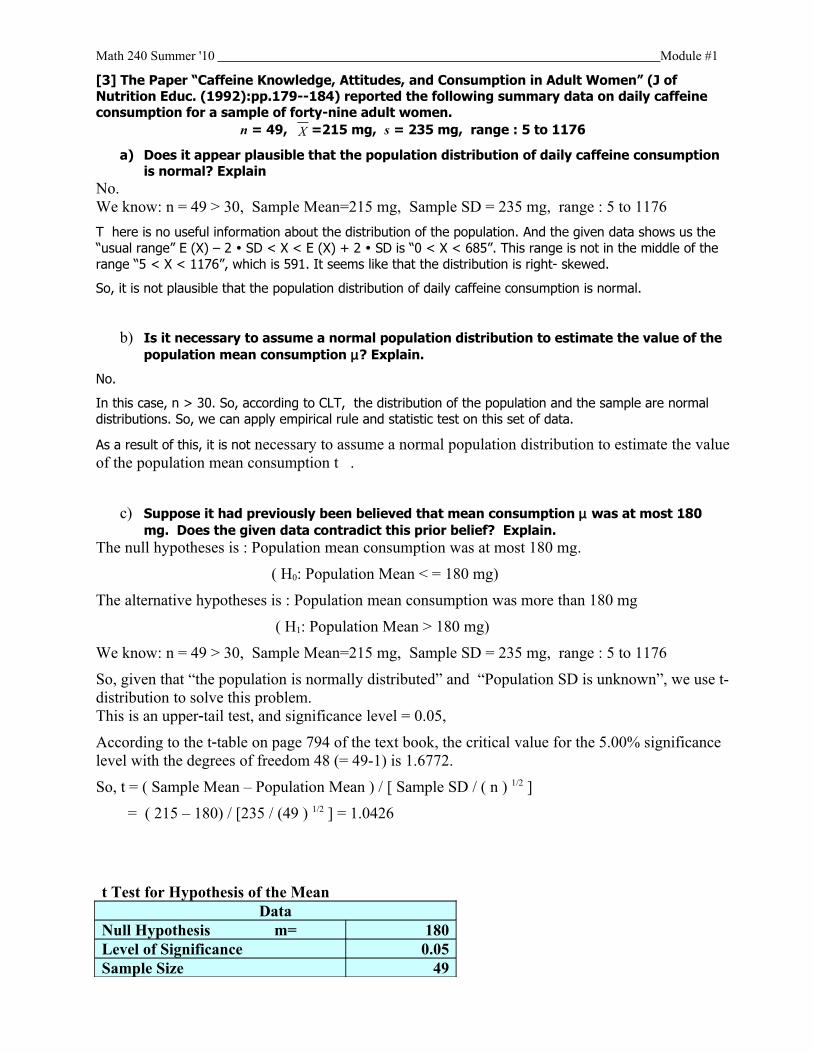
Math 240 Summer '10 Module #1
[3] The Paper “Caffeine Knowledge, Attitudes, and Consumption in Adult Women” (J of Nutrition Educ. (1992):pp.179--184) reported the following summary data on daily caffeine consumption for a sample of forty-nine adult women.
n = 49, X =215 mg, s = 235 mg, range : 5 to 1176
a) Does it appear plausible that the population distribution of daily caffeine consumption is normal? Explain
No.We know: n = 49 > 30, Sample Mean=215 mg, Sample SD = 235 mg, range : 5 to 1176
T here is no useful information about the distribution of the population. And the given data shows us the “usual range” E (X) – 2 SD < X < E (X) + 2 SD is “0 < X < 685”. This range is not in the middle of the range “5 < X < 1176”, which is 591. It seems like that the distribution is right- skewed.
So, it is not plausible that the population distribution of daily caffeine consumption is normal.
b) Is it necessary to assume a normal population distribution to estimate the value of the population mean consumption µ? Explain.
No.
In this case, n > 30. So, according to CLT, the distribution of the population and the sample are normal distributions. So, we can apply empirical rule and statistic test on this set of data.
As a result of this, it is not necessary to assume a normal population distribution to estimate the value of the population mean consumption t .
c) Suppose it had previously been believed that mean consumption µ was at most 180 mg. Does the given data contradict this prior belief? Explain.
The null hypotheses is : Population mean consumption was at most 180 mg.
( H0: Population Mean < = 180 mg)
The alternative hypotheses is : Population mean consumption was more than 180 mg
( H1: Population Mean > 180 mg)
We know: n = 49 > 30, Sample Mean=215 mg, Sample SD = 235 mg, range : 5 to 1176
So, given that “the population is normally distributed” and “Population SD is unknown”, we use t- distribution to solve this problem.This is an upper tail test, and significance level = 0.05, ‐According to the t table on page 794 of the text book, the critical value for the 5.00% significance‐ level with the degrees of freedom 48 (= 49-1) is 1.6772.
So, t = ( Sample Mean – Population Mean ) / [ Sample SD / ( n ) 1/2 ]
= ( 215 – 180) / [235 / (49 ) 1/2 ] = 1.0426
t Test for Hypothesis of the MeanData
Null Hypothesis m= 180Level of Significance 0.05Sample Size 49

Math 240 Summer '10 Module #1
Sample Mean 215Sample Standard Deviation 235
Intermediate CalculationsStandard Error of the Mean 33.57142857Degrees of Freedom 48t Test Statistic 1.042553191
Upper-Tail Test Upper Critical Value 1.677224197p-Value 0.151188939
Do not reject the null hypothesisBy the traditional approach (the critical value approach):The critical value is t = 1.6772 and the test statistic is t = 1.0426. Since the test statistic is smaller than the critical value (that is, the test statistic does not fall into therejection region), we fail to reject the null hypothesis.By the p value approach (the recommended approach):‐The p value is ‐ p = 0.1512 and the level of significance = 0.050. Since the p value‐is larger than the level of confidence (that is, the test statistic does not fall into the rejectionregion), we fail to reject the null hypothesis.
As a result of this, we fail to reject H0. Hence there is insufficient evidence that the claim is false. The given data do not contradict the prior belief.

Math 240 Summer '10 Module #1
[4] For drivers in the 20-24 age bracket, there is a 34% rate of car accidents in one year (based on data from the National Safety Council). An insurance investigator finds that in a group of 500 randomly selected drivers aged 20-24 living in New York City. 40% had accidents in the last year.
a) If the 34% rate is correct, estimate the probability that in a group of 500 randomly selected drivers, at least 40% had accidents in the last year.
With Population proportion = 0.34 and n = 500, the conditions n Population proportion = (500)(0.34) = 179 ≥ 5 and n (1 –Population proportion) = 500(1 – 0.34) = 330 ≥ 5. So, we can use the normal distribution to approximate a binomial distribution.The null hypotheses is : For drivers in the 20-24 age bracket, there is a 34% rate of car accidents in one year.
( H0: Population proportion = 34%)
The alternative hypotheses is : For drivers in the 20-24 age bracket, there are more than 34% of car accidents in one year.
( H1: Population proportion > 34%)
We know: n = 500 > 30, Population propotion = 34%,
p = 40%, Number of successes = 500 × 40% = 200,
This is an upper- tail test, and Level of significance = 5.00%,
For proportion case, we use Z- test statistic:
Z = ( p – Population proportion ) / [ Population proportion (1 – Population proportion) / n ] 1/2
= ( 0.40 – 0.34 ) / [ 0.34 (1 – 0.34) / 500 ] 1/2 = 2.8322
Z Test of Hypothesis for the ProportionData
Null Hypothesis p = 0.34Level of Significance 0.05Number of Successes 200Sample Size 500
Intermediate CalculationsSample Proportion 0.4Standard Error 0.0211849Z Test Statistic 2.83220592
Upper-Tail Test Upper Critical Value 1.644853627p-Value 0.002311403
Reject the null hypothesis
So, the p- Value is 0.2311%. This means “the probability that in a group of 500 randomly selected drivers, at least 40% had accidents in the last year, is 0.2311%”.

Math 240 Summer '10 Module #1
b) Based on your finding in (a), is there strong evidence supporting the claim that the accident rate in the 20-24 age bracket in New York City is higher than 34%? Explain.
By the traditional approach (the critical value approach):The critical value is 1.6450 and the test statistic is Z = 2.8322. Since the test statistic is larger than the critical value (that is, the test statistic falls into therejection region), we reject the null hypothesis.By the p‐value approach (the recommended approach):The p‐ value is p = 0.2311% and the level of significance = 5.0000%. Since the p‐valueis smaller than the level of confidence (that is, the test statistic falls into the rejectionregion), we reject the null hypothesis.
As a result of this, we reject H0. Hence there is a strong evidence that the accident rate in the 20-24 age bracket in New York City is higher than 34%.
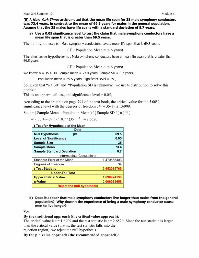
Math 240 Summer '10 Module #1
[5] A New York Times article noted that the mean life span for 35 male symphony conductors was 73.4 years, in contrast to the mean of 69.5 years for males in the general population. Assume that the 35 males have life spans with a standard deviation of 8.7 years.
a) Use a 0.05 significance level to test the claim that male symphony conductors have a mean life span that is greater than 69.5 years.
The null hypotheses is : Male symphony conductors have a mean life span that is 69.5 years.
( H1: Population Mean = 69.5 years)
The alternative hypotheses is : Male symphony conductors have a mean life span that is greater than 69.5 years.
( H1: Population Mean > 69.5 years)
We know: n = 35 > 30, Sample mean = 73.4 years, Sample SD = 8.7 years,
Population mean = 69.5 years, Significant level = 5%,
So, given that “n > 30” and “Population SD is unknown”, we use t- distribution to solve this problem.This is an upper- tail test, and significance level = 0.05,
According to the t‐table on page 794 of the text book, the critical value for the 5.00% significance level with the degrees of freedom 34 (= 35-1) is 1.6909.
So, t = ( Sample Mean – Population Mean ) / [ Sample SD / ( n ) 1/2 ]
= ( 73.4 – 69.5) / [8.7 / (35 ) 1/2 ] = 2.6520
t Test for Hypothesis of the MeanData
Null Hypothesis µ= 69.5Level of Significance 0.05Sample Size 35Sample Mean 73.4Sample Standard Deviation 8.7
Intermediate CalculationsStandard Error of the Mean 1.470568403Degrees of Freedom 34t Test Statistic 2.652035765
Upper-Tail Test Upper Critical Value 1.690924198p-Value 0.006033658
Reject the null hypothesis
b) Does it appear that male symphony conductors live longer than males from the general population? Why doesn’t the experience of being a male symphony conductor cause men to live longer?
Yes.By the traditional approach (the critical value approach):The critical value is t = 1.6909 and the test statistic is t = 2.6520. Since the test statistic is larger than the critical value (that is, the test statistic falls into therejection region), we reject the null hypothesis.By the p‐value approach (the recommended approach):

Math 240 Summer '10 Module #1
The p‐value is p = 0.6034% and the level of significance = 5.0000%. Since the p‐valueis smaller than the level of confidence (that is, the test statistic falls into the rejectionregion), we reject the null hypothesis.
As a result of this, we reject H0. This means the statement is no longer ture. It appears that male symphony conductors live longer than males from the general population.
The experience of being a male symphony conductor does not cause men to live longer because this problem is related to other factors. The length of male’s life is independent. Working pressure, health problem, family issue, and other various kinks of factors also have significant impact on the length of male’s life. Additionally, being a male symphony conductor is only one tiny reason of all the factors. Not all males in the world are symphony conductor. The amount of male who are gymphony conductor is just a small sample of the population. As a consequence, the experience of being a male symphony conductor does not cause men to live longer

Math 240 Summer '10 Module #1
[6] A shop manual gives 6.5 hours as the average time required to perform a 30,000 mile major maintenance service on a Porsche 911. Last month a mechanic performed 11 such services, and his required times were as follows.
6.3 6.6 6.7 5.9 6.3 6.0 6.5 6.1 6.2 6.4 6.3
At the 2% level of significance, is there sufficient evidence to conclude that the mechanic can perform this service in less time than specified by the service manual?
Normal Probability Plot
5.8
6
6.2
6.4
6.6
6.8
-2 -1.5 -1 -0.5 0 0.5 1 1.5
Z Value
Hours
As can be seen, these points are approximately straight. So the given data are approximately
normally distributed.
Then we input the data into descriptive statistics of data analysis, we can get the following results:Sample Mean
6.3
Median 6.3Mode 6.3
SD0.24494
9So, Mean = Median = Mode proof that the distribution of normally distribution.
Sample Mean = 6.3 hours, Sample SD = 0.25.
We also know: Significance level = 2%, Pulation mean = 6.5 hours, n = 11 < 30,
The null hypotheses is : The mechanic can perform this service in 6.5 hours.
( H1: Population Mean = 6.5 hours)
The alternative hypotheses is : The mechanic can perform this service in less than 6.5 hours.
( H1: Population Mean < 6.5 hours)

Math 240 Summer '10 Module #1
So, given that “the distribution of population is normally distributed” and “Population SD is unknown”, we use t- distribution to solve this problem.This is an lower- tail test, and significance level = 0.02,
So, t = ( Sample Mean – Population Mean ) / [ Sample SD / ( n ) 1/2 ]
= ( 6.3 – 6.5) / [0.25/ (11) 1/2 ] = - 2.7080
t Test for Hypothesis of the MeanData
Null Hypothesis µ= 6.5Level of Significance 0.02Sample Size 11Sample Mean 6.3Sample Standard Deviation 0.244948974
Intermediate CalculationsStandard Error of the Mean 0.073854895Degrees of Freedom 10t Test Statistic -2.708012802
Lower-Tail Test Lower Critical Value -2.35931462p-Value 0.011004278
Reject the null hypothesisBy the traditional approach (the critical value approach):The critical value is t = - 2.3593 and the test statistic is t = - 2.7080. Since the test statistic is smaller than the critical value (that is, the test statistic falls into therejection region), we reject the null hypothesis.By the p‐value approach (the recommended approach):The p‐value is p = 1.100% and the level of significance = 2.0000%. Since the p‐valueis smaller than the level of confidence (that is, the test statistic falls into the rejectionregion), we reject the null hypothesis.
As a result of this, we reject H0. This means the statement is no longer ture. There is sufficient evidence to conclude that the mechanic can perform this service in less time than specified by the service manual.
[1] Suppose that the following information is obtained from students upon exiting the campus bookstore during the first week of classes:
k) Amount of money spent on books
l) Number of textbooks purchased
m) Amount of time spent shopping in the bookstore
n) Academic major
o) Gender
p) Ownership of a laptop computer
q) Ownership of an MP3 player
r) Number of units registered for in the current semester
s) Whether or not any clothing items were purchased at the bookstore
t) Method of payment
Classify each of the measurements as nominal, ordinal, interval, ratio scales, discrete or continuous.

Math 240 Summer '10 Module #1
qualitative quantitative
nominal ordinal interval ratio discrete continuousa) Yes Yesb) Yes Yesc) Yes Yesd) Yese) Yesf) Yesg) Yesh) Yes Yesi) Yesj) Yes
In general, is the measurement “amount of money spent on something” a continuous or discrete variable? Discuss it briefly in your own words.
According to the text book, discrete variable can be an integer of a counting process, while continuous variable can be both an integer and a continuum of a measuring process by measuring instruments with different precision.
In this case, the amount of money spent on something can only be an integer that can be counted. For instance, peple count money as intergers because we don’t have cash that has countless number. So it doesn’t have relationship with a measuring process. Therefore, I regard “amount of money spent on something” is a discrete variable.

Math 240 Summer '10 Module #1
[2] The director of market research at a large department store chain wanted to conduct a survey throughout a metropolitan area to determine the amount of time working women spend shopping for clothing in a typical month.
c) Describe both the population and the sample of interest, and indicate the type of data the director might want to collect.
1) In this survey, the population of interest is all the working women throughout the metropolitan, and the sample of interest is some of those working women that are chosen to participate in the survey. The sample is part of the population.
2) The director of market research wanted to use the data for his analysis, so he is the data collector. In other words, the data comes from primary sources. In addition, because the director wanted to conduct the survey, the data can be identified as a survey from primary sources. In the survey, the director can ask questions about beliefs, attitudes, behaviors, and other characteristics of respondents.
d) Develop a first draft of the questionnaire needed in (a) by writing a series of three categorical questions and three numerical questions that you feel would be appropriate for this survey.
1) 3 categorical questions:
(1) Do you think you are rich?
Yes/No
(2) Do you care more about your dressing than other working women?
Yes/No
(3) What type of body shape do you have?
A. Fat;
B. Normal;
C. Thin
2) 3 numerical questions:
(1) How many clothes do you try in each clothes shop?
A. 0;
B. 1 or 2;
C. 3-5;
D. more than 5
(2) What’s the highest price of one clothing you can afford?
A. Less than $50;
B. $50- $100;
C. $100- $200;
D. More than $200
(3) How much time do you spend on considering buying one clothing?
A. In 1 min;
B. 2min- 5min;
C. 5min-15min;
D. More the 15min

Math 240 Summer '10 Module #1
[3] America Online posted this question on its Web site: “How much stock do you put in long-range weather forecasts?” Among its Web site users, 38,410 chose to respond.
d) Among the responses received, 5% answered with “a lot.” What is the actual number of responses consisting of “a lot?”
1921
e) Among the responses received, 18,053 consisted of “very little or none.” What percentage of responses consisting of “very little or none?”
47%
f) Because the sample size of 38,410 is so large, can we conclude that about 5% of the general population puts “a lot” o stock in long-range weather forecasts? Why or why not?
No.
The big size of sample size donesn’t mean that it represents the general population because the sample is only part of the general population.
The best way to estimate the general population is to select large number of sample size radomly and then analysz them. If almost all of the results of the sample size have similar estimation, then the sample size can tell us the most creditable estimation about the general population.
However, in this case, it has only one estimation by getting one sample size. Different results still might appear if we selesct another big sample size and estimate it.
As a result, we cannot conclude that about 5% of the general population puts “a lot” o stock in long-range weather forecasts based on the big sample size.
[1] In an article in the November 1993 issue of Quality Progress, Barbara A. Cleary reports on improvements made in a software supplier’s responses to customer calls. In this article, the author states:
In an effort to improve its response time for these important customer-support-calls, an inbound telephone inquiry team was formed at PQ Systems, Inc., a software and training organization in Dayton, Ohio. The team found that 88 percent of the customers’ calls were already being answered immediate by the technical support group, but those who had to be called back had to wait an average of 56.6 minutes. No customer complaints had been registered, but the team believed that this response rate could be improved.
As part of its improvement process, the company studied the disposition of complete and incomplete calls to its technical support analysis. A call is considered complete if the customer’s problem has been resolved; otherwise the call is incomplete. Below is the summary table for the incomplete customer calls.
Action by Technical Support Analysts PercentageRequired customer to get more data 29.17Required more investigation by us 28.12Callbacks 21.87Required development assistance 12.50Required administrative help 4.17Determined as actually a new problem 4.17

Math 240 Summer '10 Module #1
a) Construct a Pareto chart

Math 240 Summer '10 Module #1
The Pareto Diagram for Technical Support Analysts
0.00%
5.00%
10.00%
15.00%
20.00%
25.00%
30.00%
35.00%R
equi
red
cust
omer
to g
et m
ore
data
Req
uire
d m
ore
inve
stig
atio
n by
us
Cal
lbac
ks
Req
uire
d de
velo
pmen
t ass
istan
ceR
equi
red
adm
inist
rativ
e he
lp
Det
erm
ined
as a
ctua
lly a
new
pro
blem
Actions
0.00%
10.00%
20.00%
30.00%
40.00%
50.00%
60.00%
70.00%
80.00%
90.00%
100.00%
d) What percentage of incomplete calls required “more investigation” by the analyst or “administrative
help?”
According to the given information, 28.12%of incomplete calls required “more investigation” by the
analyst, and 4.17% of incomplete calls required “administrative help”. As a result, the percentage of
incomplete calls required “more investigation” by the analyst or “administrative help” is the sum of the
persentages of “more investigation” and “administrative help”, which is : 28.12% + 4.17% = 32.29%.
d) Can you make a suggestion to improve responses?
The majority of incomplete calls required “more data” from customer and “more investigation” by the analyst. So, communication between analyst and customers can solve the problem efficiently.

Math 240 Summer '10 Module #1
[2] Do the problem 3.35 on p.126. This problem is intended for you to learn EDA (Exploratory Data Analysis).
a))
Five-number Summary for the Yield of the Money Market Account, One-Year CD, and a Five-Year CD
Money Market Account One-Year CD Five-Year CD
Minimum 0.1 1.55 3.15
First Quartile 0.5 3.05 3.9
Median 0.65 3.525 4.09
Third Quartile 1.01 4 4.35
Maximum 2.27 4.6 5.12
b)
Box-and-Whisker Plot for the Yield of the Money Market Account, One- Year CD, a Five- Year CD.
Money Market
One-Year CD
Five-Year CD
0 1 2 3 4 5 6
e) Both of the distribution of the money market account and the five-year CD are right-skewed, and the distribution of the one-year CD is left-skewed. But the distribution of the five- year CD is closed to a bell- shaped distribution.

Math 240 Summer '10 Module #1
Money market: Minimum = 0.1. Maximum = 2.27
Q1 – (IQR × 1.5) = Q1 – [(Q3 – Q1) × 1.5] = 0.5 – [ ( 1.01 – 0.5) × 1.5] = -0.265 Q3 + (IQR × 1.5) = Q3 + [(Q3 – Q1) × 1.5] = 1.01 + [ ( 1.01 – 0.5) × 1.5] = 1.775 So, Q1 – (IQR × 1.5) < the minimum < Q3 + (IQR × 1.5) < the maximumAs a result, the maximum value 2.27 is an outlier.
One-year CD:Minimum = 1.55
Maximum = 4.6Q1 – (IQR × 1.5) = Q1 – [(Q3 – Q1) × 1.5] = 3.05 – [ ( 4 – 3.05) × 1.5] = 1.625Q3 + (IQR × 1.5) = Q3 + [(Q3 – Q1) × 1.5] = 4 + [ ( 4 – 3.05) × 1.5] = 5.425 So, the minimum < Q1 – (IQR × 1.5) < the maximum < Q3 + (IQR × 1.5) As a result, the minimum value 1.55 is an outlier.
Five-year CD:Minimum = 3.15
Maximum = 5.12Q1 – (IQR × 1.5) = Q1 – [(Q3 – Q1) × 1.5] = 3.9 – [ ( 4.35 – 3.9) × 1.5] = 3.225Q3 + (IQR × 1.5) = Q3 + [(Q3 – Q1) × 1.5] = 4.35 + [ ( 4.35 – 3.9) × 1.5] = 5.025So, the minimum < Q1 – (IQR × 1.5) < Q3 + (IQR × 1.5) < the maximumAs a result, the minimum value 3.15 and the maximum value 5.12 are outliers.
Mean Standard Deviation Coefficient of Variation
Money Market 0.8165 0.521194634 63.83%
One-Year CD 3.53675 0.677621737 19.16%
Five-Year CD 4.13475 0.390745425 9.45%
Because the coefficient of variation of the money market is the highest one, the yield of the monet market is the most variable data in the group. Then the yield of the one- year CD is less variable, and the yield of the five- year CD is the lease variable data.

Math 240 Summer '10 Module #1
[3] Maximum breadth of sample of male Egyptian skulls from 4000 B.C. and 150 A.D. (based on data from
Ancient Races of the Thebaid by Thompson and Randall-Maciver):
4000 B.C. 131 119 138 125 129 126 131 132 126 128 128 131150 A.D. 136 130 126 126 139 141 137 138 133 131 134 129
d) Find the mean, median, and mode, range, variance, and the standard deviation for each of the two samples.
4000 B.C. 150 A.D.
Mean 128.6666667 133.3333333
Median 128.5 133.5
Mode 131 126
Range 19 15
Variance 21.51515152 25.15151515
Standard Deviation 4.63844279 5.015128628
e) Compare and analyze the two data sets using descriptive measures.
Based on the data of (a), we know that:
For 4000 B.C. : Mean = E (X) = 128.6666667 (almost the same as Median),
SD = 4.63844279,
So, the “usual range” E (X) – 2 SD < X < E (X) + 2 SD is 119.39 < X < 137.95.
Only 138 and 139 is out of this range. Other datas are within this “usual range”.
For 150 A.D. : Mean = 133.3333333(almost the same as Median),
SD = 5.015128628,
So, the “usual range” E (X) – 2 SD < X < E (X) + 2 SD is 123.29 < X < 143.37.
All the datas are within this “usual range”.

Math 240 Summer '10 Module #1
f) Changes in head size over time suggest interbreeding with people from other regions. Do the head sizes appear to have changed from 4000 B.C. to 150 A. D.? Explain.
Yes.
Box-and-Whisker Plot
4000 B.C.
150 A.D.
110 120 130 140 150
As can be seen, the smallest size, the Q1, the mean size, the Q3, and the largest size of people of 150 A.D. were larger than that of people of 4000 B.C. repectively. The interbreeding with people from different areas cause different combination of gene from different race. Additionally, some gene determines the breadth of sample of male Egyptian skulls. Over a period of time, from 4000 B.C. to 150 A. D., the maximum breadth of sample of male Egyptian skulls change because their gene mixed with that of other regions.
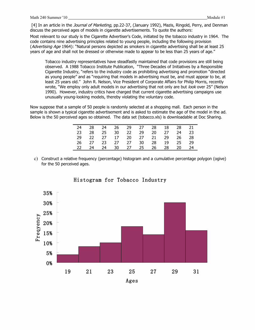
Math 240 Summer '10 Module #1
[4] In an article in the Journal of Marketing, pp.22-37, (January 1992), Mazis, Ringold, Perry, and Denman discuss the perceived ages of models in cigarette advertisements. To quote the authors:
Most relevant to our study is the Cigarette Advertiser's Code, initiated by the tobacco industry in 1964. The code contains nine advertising principles related to young people, including the following provision (Advertising Age 1964): “Natural persons depicted as smokers in cigarette advertising shall be at least 25 years of age and shall not be dressed or otherwise made to appear to be less than 25 years of age.”
Tobacco industry representatives have steadfastly maintained that code provisions are still being observed. A 1988 Tobacco Institute Publication, “Three Decades of Initiatives by a Responsible Cigarette Industry, “refers to the industry code as prohibiting advertising and promotion “directed as young people” and as “requiring that models in advertising must be, and must appear to be, at least 25 years old.” John R. Nelson, Vice President of Corporate Affairs for Philip Morris, recently wrote, “We employ only adult models in our advertising that not only are but look over 25” (Nelson 1990). However, industry critics have charged that current cigarette advertising campaigns use unusually young-looking models, thereby violating the voluntary code.
Now suppose that a sample of 50 people is randomly selected at a shopping mall. Each person in the sample is shown a typical cigarette advertisement and is asked to estimate the age of the model in the ad. Below is the 50 perceived ages so obtained. The data set (tobacco.xls) is downloadable at Doc Sharing.
24 28 24 26 29 27 28 18 28 2123 28 25 30 22 29 20 27 24 2329 22 27 17 20 27 21 29 26 2826 27 23 27 27 30 28 19 25 2922 24 24 30 27 25 26 28 20 24
c) Construct a relative frequency (percentage) histogram and a cumulative percentage polygon (ogive) for the 50 perceived ages.
Histogram for Tobacco Industry
0%
5%
10%
15%
20%
25%
30%
35%
19 21 23 25 27 29 31
Ages
Freqyency

Math 240 Summer '10 Module #1
Cumulative Percentage Polygon for Tobacco Industry
0%
10%
20%
30%
40%
50%
60%
70%
80%
90%
100%
19 21 23 25 27 29
d) What percentage of the perceived ages is below the industry's code provision (of 25 years old)? Do you think that this percentage is too high?
40% of the perceived ages are below the industry’s code provision (of 25 years old). In my opinion, this percentage is too high.
[1] A sample of 500 respondents was selected in a large metropolitan area to determine various information concerning consumer behaviors. Among the questions asked was “Do you enjoy shopping for clothing?” Of 240 males, 136 answered yes. Of 260 females, 224 answered yes.
d) Is “enjoy shopping for clothing” gender-independent? Explain.
No.
Number of RespondentsAnswers
Yes NoTotal
GenderMales 136 104 240
Females 224 36 260
Total 360 140 500 P ( enjoy ) = 360 / 500 =72% P ( male ) = 240 / 500 = 48% P ( enjoy and male ) = 136 / 500 = 27.2%

Math 240 Summer '10 Module #1
So, P ( enjoy ) P ( male ) = 72% × 48% = 34.56%,P ( enjoy | male ) = P ( enjoy and male ) / P ( male ) = 27.2% / 48% = 56.67%,
As a result, P ( enjoy ) P ( male ) is not equal to P ( enjoy and male ); P ( enjoy | male ) is not equal to P ( enjoy ), If P ( enjoy ) P ( male ) is equal to P ( enjoy and male ); P ( enjoy | male ) is equal to P ( enjoy ), then event “enjoy shopping for clothing” is gender- independent. However, in this case, the equation above cannot be achieved. So, “enjoy shopping for clothing” is not gender-independent
e) Are “enjoy shopping for clothing” and “being a male” mutually exclusive? Explain.
No.
If “enjoy shopping for clothing” and “being a male” are mutually exclusive, then P ( enjoy and male ) is equal to nothing.
However, in this case, we know “P ( enjoy and male ) = 136 / 500 = 27.2%” from (a). So, P ( enjoy and male ) is not equal to nothing. As a result of this, “enjoy shopping for clothing” and “being a male” are not mutually exclusive.
f) What is the probability that a respondent chosen at random is a male if the person answered no?
Event A: a respondent is a male
Event B: the answer of a respondent is no So, P (A) = number of males/ number of all respondents = 240/ 500 = 48%
P (B) = number of people who answered no/ number of all respondents = [(240- 136) + (260- 224)]/ 500 = (104+ 36)/ 500 = 140/ 500 = 28%
As we can seen in the chart above, P (A and B) = 104/ 500 = 20.8%Due to the face that answering no happened first as a condition, we treat this situation as
conditional probability.As a result, given the condition that the person answered no, the probability for “a
respondent chosen at random is a male” is:P (A| B) = P (A and B)/ P (B) = 20.8%/ 28% = 74.29%

Math 240 Summer '10 Module #1
[2] The sport director of a local television station surveyed a random sample of 100 viewers on their preferences regarding coverage of certain events. The survey revealed that 70 preferred coverage of San Francisco Giants' game, 26 preferred coverage of WNBA, and 6 preferred both. One of the viewers is selected at random. Find the following probabilities.
e) The viewer preferred coverage of Giants' games.
OpinionsGaints
Yes NoTotal
WNBAYes 6 20 26
No 64 10 74
Total 70 30 100In this case, assume that event A is “70 viewers preferred coverage of SF Gaint’s game”,
event B is “26 viewers preferred coverage of WNBA”.
The probability of event A is: P (A) = 70/ 100 = 70%
f) The viewer preferred at least one of coverages.
P (B) = 26/100 = 26%
P (A and B) = 6/100 = 6%
Because event A and B can happen at the same time, they are not mutually exclusive.
So, P (A or B) = P (A) + P (B) - P (A and B) = 70% + 26% - 6% = 90%
g) The viewer preferred coverage of neither event.
P (not A and not B) = 1 - P (A or B) = 1- 90% = 10%
h) The viewer preferred coverage of WNBA if he/she has already preferred coverage of Giants' games
This is a conditional probability, and the condition is event A.
As we can seen in the chart above,
P (A and B) =6/ 100 = 6%
As a result, P (B| A) = P (A and B) / P (A) = 6% / 70% = 8.57%

Math 240 Summer '10 Module #1
[3] Two baseball teams, the San Francisco Giants and the Los Angeles Dodgers, will play each other for the league championship. The Giants are, in fact the better team. (But the Dodgers have the better yell, “That's all right, that's okay. You'll be working for us someday.”) According to Brett Mullin as of April 18, 2010, the Giants have won 1162 games and the Dodgers have won 1143 games since October 18, 1889, including their days while in New York.
b) What is the probability that the Giants will win the championship if these two teams play just one game?
Assume that event A is “the Giants will win the championship”,
event B is “the Dodgers will win the championship”,
So, P (A) = 1162 / (1162+ 1143) = 1162/ 2305= 50.41%
b) What is the probability that the Giants will win the championship if these two teams play a 5-game series?
If they play a 5-game series and the Gaints will win, the number of victories for the Giants must larger than the Dodgers’. The outcomes are as follows:
(4) A happens 3 times: P ( 1 ) = [ P ( A ) ] 3
(5) A happens 3 times, while B happens 1 time: P ( 2 ) = 3 × [ P ( A ) ] 3 × P ( not A )
(6) A happens 3 times while B happens 2 times: P ( 3 ) = 6 × [ P ( A ) ] 3 × [ P ( not A ) ] 2
Because the 3 situation above are mutually exclusive,
P [ ( 1 ) or ( 2 ) or ( 3 ) ] = P ( 1 ) + P ( 2 ) + P ( 3 )
= [ P ( A ) ] 3 + 3 × [ P ( A ) ] 3 × P ( not A ) + 6 × [ P ( A ) ] 3 × [ P ( not A ) ] 2
= [ P ( A ) ] 3 + 3 × [ P ( A ) ] 3 × [ 1 - P ( A ) ] + 6 × [ P ( A ) ] 3 × [ 1 - P ( A ) ] 2
= (50.41% ) 3 + 3 ×(50.41% ) 3 × ( 1 - 50.41% ) + 6 × (50.41% ) 3 × ( 1 - 50.41% ) 2
= 50.77%
As a consequence, the probability that the Giants will win the championship if these two teams play a 5-game series is 50.77%.

Math 240 Summer '10 Module #1
[4] At a certain gas station, 40% of all customers fill their tanks. Of those who fill their tanks, 80% pay with a credit card.
c) What is the probability that a randomly selected customer fills his or her tank and pays with a credit card?
Assume that event A is “the customer fills his or her tank”, and event B is “the customer pays with a credit card”.
This is a conditional probability because the customer pay with a credit card after he or her has filled his or her tank.
So, P (A) = 40%.
P (B| A) = 80%
As a result, P (A and B) = P (B| A) × P (A) = 80% × 40% = 32%
d) If three customers are randomly selected, what is the probability that all three fill their tanks and pay with a credit card?
Due to the face that the selections happened at the same time, they are independent events.
As a result, the probability that all three fill their tanks and pay with a credit card is:
[P ( A and B ) ] 3 = ( 32% ) 3 = 3.28%

Math 240 Summer '10 Module #1
[5] The probability is 0.70 that a rare tropical disease will be treated correctly. If it is treated correctly, the probability that the patient will be cured is 0.90. If it is not treated correctly, the probability is only 0.40 that the patient will be cured.
c) What is the probability that a randomly selected patient having this disease will be cured?
Assume that event A is “the disease will be treated correctly”, event B is “the disease will be cured”.
P (A) = 70%
P (not A) = 30%
P (B| A) = 90%
P (B| not A) = 40%
According to decision tree,
(1) P (A) = 70%: P (A and B) =P (B| A) × P (A) = 90% × 70% = 63%
P (A and not B) =P (not B| A) × P (A) = [1- P (B| A)] ×P (A)
= (1- 90%) × 70% = 10% × 70% = 7%
(2) P (not A) = 30%: P (not A and B) =P (B| not A) × P (not A) = 40% × 30% = 12%
P (not A and not B) =P (not B| notA) × P (not A)
= [1- P (B| notA)] ×P (not A) = (1- 40%) × 30%
=60% × 30% = 18%
The the disease will be cured under two situation, one is “the disease is treated correctly”, another one is “the disease is not treated correctly”.
P (A and B) or P (not A and B) cannot happen at the same time. So, they are mutually exclusive.
As a result, P (B) = P (A and B) + P (not A and B) = 63% + 12% = 75%
d) Suppose that a randomly selected patient having this disease is cured, what is the probability that it was not treated correctly?
Because P(not A and B) = P(B) ×P(not A| B) = P(not A) × P(B| not A),
We can get:
P (not A| B) = P (not A) and B) / P (B) = 12%/ 75% = 16
[1] In a clinical trial of Lipitor, a common drug used to lower cholesterol, 863 patients were given a treatment of 10-mg Atorvastatin tablets. Among them, 19 patients experienced flu symptoms and 844 patients did not (based on data from Pfizer, Inc.).
e) Estimate the probability that a patient taking the drug will experience flu symptoms.
The average occurences is 19 / 863 = 2.2%
We use possion distribution.
Poisson ProbabilitiesData

Math 240 Summer '10 Module #1
Average/Expected number of successes: 0.022Poisson Probabilities Table
X P(X)1 0.021521
As a result, the probability that a patient taking the drug will experience flu symptoms is 2.15%.
f) Is this unusual for a patient taking the drug to experience flu symptoms? Explain.
It is unusual.
Mean = 0.022 = SD2
So SD = 0.15
The the “usual range” E (X) – 2 SD < X < E (X) + 2 SD is - 0.28 < X < 0.32.
However, X = 1 is out of the usual range.
As a result, it is unusual for a patient taking the drug to experience flu symptoms.
g) If you know that the probability of flu symptoms for a person not receiving any treatment is 0.019, what is the probability that there are 19 who experience flu symptoms among 863 patients? Explain.
863 people are independent.
Two outcomes are “experience flu symptomes” and “ not experience flu symptomes”
P (experience flu symptomes) = 1.9% is fixed.
So, it’s a binomial distribution.
Binomial ProbabilitiesData
Sample size 863Probability of success 0.019Binomial Probabilities Table
X P(X)19 0.075404
So, P (X = 19) = 8.54%
The probability that there are 19 who experience flu symptoms among 863 patients is 7.54%
h) Is this unusual to find that among 863 patients, there are 19 who experience flu symptoms in c)? Explain.

Math 240 Summer '10 Module #1
Histogram
0
0.02
0.04
0.06
0.08
0.1
0.12
0 2 4 6 8 10 12 14 16 18 20 22 24 26 28 30 32 34 36 38
Number of Successes
P(X)
As can be seen from the bell- shaped distribution, 19 people is in the usual range of E (X) – 2 SD < X < E (X) + 2 SD.
So, Is this not unusual to find that among 863 patients, there are 19 who experience flu symptoms.

Math 240 Summer '10 Module #1
[2] The probability distribution for collision insurance claims paid by the T. J. Automobile Insurance Company is as follows:
Claim Probability$0 0.90$500 0.04$1000 0.03$2000 0.01$3000 0.01$4000 0.01
c) Use the expected collision claim amount to determine the collision insurance premium that would allow the company to break even on the collision portion of the policy.
E (X) = $500 × 4% + $1000 × 3% + ($2000 + $3000 + $4000) × 1%
= $20 +$30 +$90 = $140
d) The insurance company charges an annual rate of $250 for the collision coverage. What is the expected value of the collision policy for the policy holder? Why does the policyholder purchase a collision policy with this expected value?
E (X) = ($0 - $250) × 90% + ($500 - $250) × 4% + ($1000 - $250) × 3%
+ [($2000 + $3000 + $4000) – (3 × $250)] × 1%
= - $225 + $10 + $22.5 + $82.5 = - $110
The policyholder purchase a collision policy with this expected value because he need to pay out less amount of money.
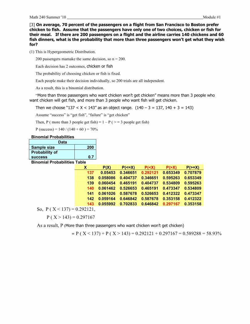
Math 240 Summer '10 Module #1
[3] On average, 70 percent of the passengers on a flight from San Francisco to Boston prefer chicken to fish. Assume that the passengers have only one of two choices, chicken or fish for their meal. If there are 200 passengers on a flight and the airline carries 140 chickens and 60 fish dinners, what is the probability that more than three passengers won’t get what they wish for?
(1) This is Hypergeometric Distribution.
200 passengers mamake the same decision, so n = 200.
Each decision has 2 outcomes, chicken or fish
The probability of choosing chicken or fish is fixed.
Each people make their decision individually, so 200 trials are all independent.
As a result, this is a binomial distribution.
“More than three passengers who want chicken won’t get chicken” means more than 3 people who want chicken will get fish, and more than 3 people who want fish will get chicken.
Then we choose “137 < X < 143” as an object range. (140 – 3 = 137, 140 + 3 = 143)
Assume “success” is “get fish”, “failure” is “get chicken”
Then, P ( more than 3 people get fish) = 1 – P ( > = 3 people get fish)
P (success) = 140 / (140 + 60 ) = 70%
Binomial ProbabilitiesData
Sample size 200Probability of success 0.7Binomial Probabilities Table
X P(X) P(<=X) P(<X) P(>X) P(>=X)137 0.05453 0.346651 0.292121 0.653349 0.707879138 0.058086 0.404737 0.346651 0.595263 0.653349139 0.060454 0.465191 0.404737 0.534809 0.595263140 0.061462 0.526653 0.465191 0.473347 0.534809141 0.061026 0.587678 0.526653 0.412322 0.473347142 0.059164 0.646842 0.587678 0.353158 0.412322143 0.055992 0.702833 0.646842 0.297167 0.353158
So, P ( X < 137) = 0.292121,
P ( X > 143) = 0.297167
As a result, P (More than three passengers who want chicken won’t get chicken)
= P ( X < 137) + P ( X > 143) = 0.292121 + 0.297167 = 0.589288 = 58.93%

Math 240 Summer '10 Module #1
[4] Mario’s Pizza Parlor has just opened. Due to a lack of employee training, there is only a 0.90 probability that a pizza will be edible. An order for five pizzas has just been placed. What is the minimum number of pizzas that must be made in order to be least 99% sure that there will be five that are edible?
Each pizza is independent. P (edible) = 0.90 is fixed.Two outcomes are “edible” and “not edible”So, it’s a binomial distribution.We also have P( X > = 5 ) = 99%.(1)Assume the number of trials is 5: P( X > = 5 ) = 59.05% has not reached 99%. Binomial Probabilities
DataSample size 5Probability of success 0.9Binomial Probabilities Table
X P(X) P(<=X) P(<X) P(>X) P(>=X)5 0.59049 1 0.40951 0 0.59049
(2)Assume the number of trials is 6: P( X > = 5 ) = 88.57% has not reached 99%. Binomial Probabilities
DataSample size 6Probability of success 0.9Binomial Probabilities Table
X P(X) P(<=X) P(<X) P(>X) P(>=X)5 0.354294 0.468559 0.114265 0.531441 0.885735
(3)Assume the number of trials is 7: P( X > = 5 ) = 97.43% has not reached 99%. Binomial Probabilities
DataSample size 7Probability of success 0.9Binomial Probabilities Table
X P(X) P(<=X) P(<X) P(>X) P(>=X)5 0.124003 0.149694 0.025692 0.850306 0.974309
(4)Assume the number of trials is 8: P( X > = 5 ) = 99.50 has reached 99%. Binomial Probabilities
DataSample size 8Probability of success 0.9Binomial Probabilities Table
X P(X) P(<=X) P(<X) P(>X) P(>=X)5 0.033067 0.038092 0.005024 0.961908 0.994976
As a result, the minimum number of pizzas that must be made in order to be least 99% sure that there will be five that are edible is 8.

Math 240 Summer '10 Module #1
[5] You are the owner of a small lawn and garden service in Minneapolis. You are going to buy a new snow thrower and wish to assess the chance of receiving a complete purchase price rebate from the Taro Company. Taro's advertisements state that the company will refund the entire price of a machine if this winter's snow fall is less than 20% of the local average snowfall. The weather service reports that the average snowfall in your area is 46.0 inches, with the standard deviation of 15.2 inches based on the normal distribution. How likely is it that this rebate will happen?
Mean = E (X) = 46.0Standard Deviation = 15.220% of the local average snowfall = 20% × 46 = 9.2 inchesNormal Probabilities
Common DataMean 46Standard Deviation 15.2
Probability for X <=X Value 9.2Z Value -2.421053P(X<=9.2) 0.0077378Because SD 2 = Z 2, SD = 2.421053So the usual range “E (X) – 2 SD < X < E (X) + 2 SD” for snowfall is “41.157894 < X < 50.842106”
However, 9.2 inches is not in this range, so this rebate will not happen.
[1] A soft-drink manufacturer claims that its 12-ounce cans do not contain, on average, more than 30 calories. A random sample of 16 cans of this soft drink, which were checked for calories, contained a mean of 31.8 calories with a standard deviation of 3 calories. Assume that the number of calories in 12-ounce soda cans is normally distributed.
f) State the null and alternative hypotheses.
The null hypotheses is : 12-ounce cans do not contain more than 30 calories on average
( H0: Population Mean < = 30 calories)
The alternative hypotheses is : 12-ounce cans contain more than 30 calories on average
( H1: Population Mean > 30 calories)
g) Select the distribution to use. Explain briefly why you selected it.
I select t- distribution.
We know that the population distribution is normal distribution, so the sample population is also normally distributed.
n = 16 < 30, Sample Mean = 31.8 calories, Sample SD = 3 calories, and the population SD is unknown.
As a result, knowing “the sample is normally distributed” and “population SD is unknown”, we use t- distribution.
h) Assuming that they wish to test the claim at α = 0.025, determine the rejection and non rejection regions based on your hypotheses in a). State the critical value.

Math 240 Summer '10 Module #1
Significance level = 0.025,
This is an upper‐tail test. According to the t‐table on page 794 of the text book, the critical value for the 2.5% significance level with the degrees of freedom 15 (= 16-1) is 2.1315.
i) Calculate the value of the test statistic.
Population Mean = 30 calories,
n = 16, Sample Mean = 31.8 calories, Sample SD = 3 calories,
So, t = ( Sample Mean – Population Mean ) / [ Sample SD / ( n ) 1/2 ] = ( 31.8 – 30) / [3 / (16 ) 1/2 ]
= 1.8 / (3/4) = 2.4
t Test for Hypothesis of the MeanData
Null Hypothesis µ= 30Level of Significance 0.025Sample Size 16Sample Mean 31.8Sample Standard Deviation 3
Intermediate CalculationsStandard Error of the Mean 0.75Degrees of Freedom 15t Test Statistic 2.4
Upper-Tail Test
Upper Critical Value 2.131449536p-Value 0.014912465
Reject the null hypothesis
j) Does the sample information support that the manufacturer's claim is false? Explain your conclusion in words.
Yes. By the traditional approach (the critical value approach):The critical value is t = 2.1215 and the test statistic is t = 2.4. Since the test statistic is larger than the critical value (that is, the test statistic falls into therejection region), we reject the null hypothesis.By the p‐value approach (the recommended approach):The p‐ value is p = 0.0149 and the level of significance = 0.025. Since the p‐valueis smaller than the level of confidence (that is, the test statistic falls into the rejectionregion), we reject the null hypothesis.
As a result of this, we reject H0. Hence there are sufficient evidences that the manufacturer's claim is false.

Math 240 Summer '10 Module #1
[2] In March 16, 1998, issue of Fortune magazine, the results of a survey of 2,221 MBA students from across the United States conducted by the Stockholm-based academic consulting firm Universum showed that only 20 percent of MBA students expect to stay at their first job five years or more. Source: Shalley Branch, "MBAs: What Do They Really Want," Fortune (March 16, 1998), p.167.
c) Assuming that a random sample was employed, test hypotheses at the 2% level of significance for the proportion 25% of all U.S. MBA students who expect to stay at their first job five years or more.
With Population proportion = 0.25 and n = 2,221, the conditions n Population proportion = (2,221)(0.25) = 555.25 ≥ 5 and n (1 –Population proportion) = 2,221(1 – 0.25) = 1,665.75 ≥ 5. So, we can use the normal distribution to approximate a binomial distribution.
The null hypotheses is : the proportion of all U.S. MBA students who expect to stay at their first job five years or more is 25%.
( H0: Population proportion = 25%)
The alternative hypotheses is : the proportion of all U.S. MBA students who expect to stay at their first job five years or more is not 25%.
( H1: Population proportion < 25%)
We know :n = 2,221 > 30, p = 20%, Level of significance = 2.00%, Population proportion = 25%,For proportion case, we use Z- test statistic:
Z = ( p – Population proportion ) / [ Population proportion (1 – Population proportion) / n ] 1/2
= ( 0.20 – 0.25 ) / [ 0.25 (1 – 0.25) / 2,221 ] 1/2 = - 5.4026
By PHStat:
Population proportion = 25%, Level of significance = 2.00%, Number of successes = 2,221 × 20% = 444.2, n = 2,221
Z Test of Hypothesis for the ProportionData
Null Hypothesis π = 0.25Level of Significance 0.02Number of Successes 445Sample Size 2221
Intermediate CalculationsSample Proportion 0.200360198Standard Error 0.009188114Z Test Statistic -5.402610805
Lower-Tail Test
Lower Critical Value -2.053748911p-Value 3.28389E-08
Reject the null hypothesis
d) Based on the interval from a), is there strong evidence that less than one-fourth of all U.S. MBA students expect to stay?
By the traditional approach (the critical value approach):The critical value is - 2.0537 and the test statistic is Z = - 5.4026. Since the test statistic is less than the critical value (that is, the test statistic falls into the

Math 240 Summer '10 Module #1
rejection region), we reject the null hypothesis.By the p‐value approach (the recommended approach):The p‐ value is p = 3.28389E-08 and the level of significance = 0.02. Since the p‐valueis smaller than the level of confidence (that is, the test statistic falls into the rejectionregion), we reject the null hypothesis.
As a result of this, we reject H0. Hence there are sufficient evidences that the proportion of all U.S. MBA students who expect to stay at their first job five years or more is less than 25%.

Math 240 Summer '10 Module #1
[3] The Paper “Caffeine Knowledge, Attitudes, and Consumption in Adult Women” (J of Nutrition Educ. (1992):pp.179--184) reported the following summary data on daily caffeine consumption for a sample of forty-nine adult women.
n = 49, X =215 mg, s = 235 mg, range : 5 to 1176
d) Does it appear plausible that the population distribution of daily caffeine consumption is normal? Explain
No.We know: n = 49 > 30, Sample Mean=215 mg, Sample SD = 235 mg, range : 5 to 1176
T here is no useful information about the distribution of the population. And the given data shows us the “usual range” E (X) – 2 SD < X < E (X) + 2 SD is “0 < X < 685”. This range is not in the middle of the range “5 < X < 1176”, which is 591. It seems like that the distribution is right- skewed.
So, it is not plausible that the population distribution of daily caffeine consumption is normal.
e) Is it necessary to assume a normal population distribution to estimate the value of the population mean consumption µ? Explain.
No.
In this case, n > 30. So, according to CLT, the distribution of the population and the sample are normal distributions. So, we can apply empirical rule and statistic test on this set of data.
As a result of this, it is not necessary to assume a normal population distribution to estimate the value of the population mean consumption t .
f) Suppose it had previously been believed that mean consumption µ was at most 180 mg. Does the given data contradict this prior belief? Explain.
The null hypotheses is : Population mean consumption was at most 180 mg.
( H0: Population Mean < = 180 mg)
The alternative hypotheses is : Population mean consumption was more than 180 mg
( H1: Population Mean > 180 mg)
We know: n = 49 > 30, Sample Mean=215 mg, Sample SD = 235 mg, range : 5 to 1176
So, given that “the population is normally distributed” and “Population SD is unknown”, we use t- distribution to solve this problem.This is an upper tail test, and significance level = 0.05, ‐According to the t table on page 794 of the text book, the critical value for the 5.00% significance‐ level with the degrees of freedom 48 (= 49-1) is 1.6772.
So, t = ( Sample Mean – Population Mean ) / [ Sample SD / ( n ) 1/2 ]
= ( 215 – 180) / [235 / (49 ) 1/2 ] = 1.0426
t Test for Hypothesis of the MeanData
Null Hypothesis m= 180Level of Significance 0.05Sample Size 49

Math 240 Summer '10 Module #1
Sample Mean 215Sample Standard Deviation 235
Intermediate CalculationsStandard Error of the Mean 33.57142857Degrees of Freedom 48t Test Statistic 1.042553191
Upper-Tail Test Upper Critical Value 1.677224197p-Value 0.151188939
Do not reject the null hypothesisBy the traditional approach (the critical value approach):The critical value is t = 1.6772 and the test statistic is t = 1.0426. Since the test statistic is smaller than the critical value (that is, the test statistic does not fall into therejection region), we fail to reject the null hypothesis.By the p value approach (the recommended approach):‐The p value is ‐ p = 0.1512 and the level of significance = 0.050. Since the p value‐is larger than the level of confidence (that is, the test statistic does not fall into the rejectionregion), we fail to reject the null hypothesis.
As a result of this, we fail to reject H0. Hence there is insufficient evidence that the claim is false. The given data do not contradict the prior belief.

Math 240 Summer '10 Module #1
[4] For drivers in the 20-24 age bracket, there is a 34% rate of car accidents in one year (based on data from the National Safety Council). An insurance investigator finds that in a group of 500 randomly selected drivers aged 20-24 living in New York City. 40% had accidents in the last year.
c) If the 34% rate is correct, estimate the probability that in a group of 500 randomly selected drivers, at least 40% had accidents in the last year.
With Population proportion = 0.34 and n = 500, the conditions n Population proportion = (500)(0.34) = 179 ≥ 5 and n (1 –Population proportion) = 500(1 – 0.34) = 330 ≥ 5. So, we can use the normal distribution to approximate a binomial distribution.The null hypotheses is : For drivers in the 20-24 age bracket, there is a 34% rate of car accidents in one year.
( H0: Population proportion = 34%)
The alternative hypotheses is : For drivers in the 20-24 age bracket, there are more than 34% of car accidents in one year.
( H1: Population proportion > 34%)
We know: n = 500 > 30, Population propotion = 34%,
p = 40%, Number of successes = 500 × 40% = 200,
This is an upper- tail test, and Level of significance = 5.00%,
For proportion case, we use Z- test statistic:
Z = ( p – Population proportion ) / [ Population proportion (1 – Population proportion) / n ] 1/2
= ( 0.40 – 0.34 ) / [ 0.34 (1 – 0.34) / 500 ] 1/2 = 2.8322
Z Test of Hypothesis for the ProportionData
Null Hypothesis p = 0.34Level of Significance 0.05Number of Successes 200Sample Size 500
Intermediate CalculationsSample Proportion 0.4Standard Error 0.0211849Z Test Statistic 2.83220592
Upper-Tail Test Upper Critical Value 1.644853627p-Value 0.002311403
Reject the null hypothesis
So, the p- Value is 0.2311%. This means “the probability that in a group of 500 randomly selected drivers, at least 40% had accidents in the last year, is 0.2311%”.

Math 240 Summer '10 Module #1
d) Based on your finding in (a), is there strong evidence supporting the claim that the accident rate in the 20-24 age bracket in New York City is higher than 34%? Explain.
By the traditional approach (the critical value approach):The critical value is 1.6450 and the test statistic is Z = 2.8322. Since the test statistic is larger than the critical value (that is, the test statistic falls into therejection region), we reject the null hypothesis.By the p‐value approach (the recommended approach):The p‐ value is p = 0.2311% and the level of significance = 5.0000%. Since the p‐valueis smaller than the level of confidence (that is, the test statistic falls into the rejectionregion), we reject the null hypothesis.
As a result of this, we reject H0. Hence there is a strong evidence that the accident rate in the 20-24 age bracket in New York City is higher than 34%.

Math 240 Summer '10 Module #1
[5] A New York Times article noted that the mean life span for 35 male symphony conductors was 73.4 years, in contrast to the mean of 69.5 years for males in the general population. Assume that the 35 males have life spans with a standard deviation of 8.7 years.
c) Use a 0.05 significance level to test the claim that male symphony conductors have a mean life span that is greater than 69.5 years.
The null hypotheses is : Male symphony conductors have a mean life span that is 69.5 years.
( H1: Population Mean = 69.5 years)
The alternative hypotheses is : Male symphony conductors have a mean life span that is greater than 69.5 years.
( H1: Population Mean > 69.5 years)
We know: n = 35 > 30, Sample mean = 73.4 years, Sample SD = 8.7 years,
Population mean = 69.5 years, Significant level = 5%,
So, given that “n > 30” and “Population SD is unknown”, we use t- distribution to solve this problem.This is an upper- tail test, and significance level = 0.05,
According to the t‐table on page 794 of the text book, the critical value for the 5.00% significance level with the degrees of freedom 34 (= 35-1) is 1.6909.
So, t = ( Sample Mean – Population Mean ) / [ Sample SD / ( n ) 1/2 ]
= ( 73.4 – 69.5) / [8.7 / (35 ) 1/2 ] = 2.6520
t Test for Hypothesis of the MeanData
Null Hypothesis µ= 69.5Level of Significance 0.05Sample Size 35Sample Mean 73.4Sample Standard Deviation 8.7
Intermediate CalculationsStandard Error of the Mean 1.470568403Degrees of Freedom 34t Test Statistic 2.652035765
Upper-Tail Test Upper Critical Value 1.690924198p-Value 0.006033658
Reject the null hypothesis
d) Does it appear that male symphony conductors live longer than males from the general population? Why doesn’t the experience of being a male symphony conductor cause men to live longer?
Yes.By the traditional approach (the critical value approach):The critical value is t = 1.6909 and the test statistic is t = 2.6520. Since the test statistic is larger than the critical value (that is, the test statistic falls into therejection region), we reject the null hypothesis.By the p‐value approach (the recommended approach):
Math 240 Summer '10 Module #1
The p‐value is p = 0.6034% and the level of significance = 5.0000%. Since the p‐valueis smaller than the level of confidence (that is, the test statistic falls into the rejectionregion), we reject the null hypothesis.
As a result of this, we reject H0. This means the statement is no longer ture. It appears that male symphony conductors live longer than males from the general population.
The experience of being a male symphony conductor does not cause men to live longer because this problem is related to other factors. The length of male’s life is independent. Working pressure, health problem, family issue, and other various kinks of factors also have significant impact on the length of male’s life. Additionally, being a male symphony conductor is only one tiny reason of all the factors. Not all males in the world are symphony conductor. The amount of male who are gymphony conductor is just a small sample of the population. As a consequence, the experience of being a male symphony conductor does not cause men to live longer

Math 240 Summer '10 Module #1
[6] A shop manual gives 6.5 hours as the average time required to perform a 30,000 mile major maintenance service on a Porsche 911. Last month a mechanic performed 11 such services, and his required times were as follows.
6.3 6.6 6.7 5.9 6.3 6.0 6.5 6.1 6.2 6.4 6.3
At the 2% level of significance, is there sufficient evidence to conclude that the mechanic can perform this service in less time than specified by the service manual?
Normal Probability Plot
5.8
6
6.2
6.4
6.6
6.8
-2 -1.5 -1 -0.5 0 0.5 1 1.5
Z Value
Hours
As can be seen, these points are approximately straight. So the given data are approximately
normally distributed.
Then we input the data into descriptive statistics of data analysis, we can get the following results:Sample Mean
6.3
Median 6.3Mode 6.3
SD0.24494
9So, Mean = Median = Mode proof that the distribution of normally distribution.
Sample Mean = 6.3 hours, Sample SD = 0.25.
We also know: Significance level = 2%, Pulation mean = 6.5 hours, n = 11 < 30,
The null hypotheses is : The mechanic can perform this service in 6.5 hours.
( H1: Population Mean = 6.5 hours)
The alternative hypotheses is : The mechanic can perform this service in less than 6.5 hours.
( H1: Population Mean < 6.5 hours)

Math 240 Summer '10 Module #1
So, given that “the distribution of population is normally distributed” and “Population SD is unknown”, we use t- distribution to solve this problem.This is an lower- tail test, and significance level = 0.02,
So, t = ( Sample Mean – Population Mean ) / [ Sample SD / ( n ) 1/2 ]
= ( 6.3 – 6.5) / [0.25/ (11) 1/2 ] = - 2.7080
t Test for Hypothesis of the MeanData
Null Hypothesis µ= 6.5Level of Significance 0.02Sample Size 11Sample Mean 6.3Sample Standard Deviation 0.244948974
Intermediate CalculationsStandard Error of the Mean 0.073854895Degrees of Freedom 10t Test Statistic -2.708012802
Lower-Tail Test Lower Critical Value -2.35931462p-Value 0.011004278
Reject the null hypothesisBy the traditional approach (the critical value approach):The critical value is t = - 2.3593 and the test statistic is t = - 2.7080. Since the test statistic is smaller than the critical value (that is, the test statistic falls into therejection region), we reject the null hypothesis.By the p‐value approach (the recommended approach):The p‐value is p = 1.100% and the level of significance = 2.0000%. Since the p‐valueis smaller than the level of confidence (that is, the test statistic falls into the rejectionregion), we reject the null hypothesis.
As a result of this, we reject H0. This means the statement is no longer ture. There is sufficient evidence to conclude that the mechanic can perform this service in less time than specified by the service manual.