statistics 371, lecture 3
TRANSCRIPT
Outline
1 The Binomial distributionProbability distributionAssumptionsMean and Standard deviation
2 The Normal DistributionIntroductionA particular case: the standard normalGeneral form
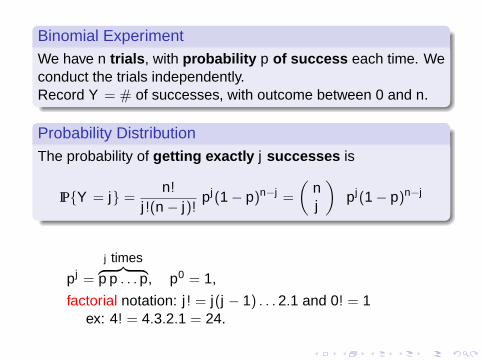
Binomial ExperimentWe have n trials , with probability p of success each time. Weconduct the trials independently.Record Y = # of successes, with outcome between 0 and n.
Probability DistributionThe probability of getting exactly j successes is
IP{Y = j} =n!
j!(n − j)!pj(1− p)n−j =
(nj
)pj(1− p)n−j
pj =
j times︷ ︸︸ ︷p p . . . p, p0 = 1,
factorial notation: j! = j(j − 1) . . . 2.1 and 0! = 1ex: 4! = 4.3.2.1 = 24.
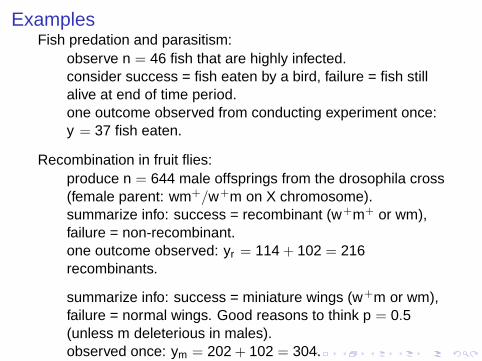
ExamplesFish predation and parasitism:
observe n = 46 fish that are highly infected.consider success = fish eaten by a bird, failure = fish stillalive at end of time period.one outcome observed from conducting experiment once:y = 37 fish eaten.
Recombination in fruit flies:produce n = 644 male offsprings from the drosophila cross(female parent: wm+/w+m on X chromosome).summarize info: success = recombinant (w+m+ or wm),failure = non-recombinant.one outcome observed: yr = 114 + 102 = 216recombinants.
summarize info: success = miniature wings (w+m or wm),failure = normal wings. Good reasons to think p = 0.5(unless m deleterious in males).observed once: ym = 202 + 102 = 304.
Calculation examples
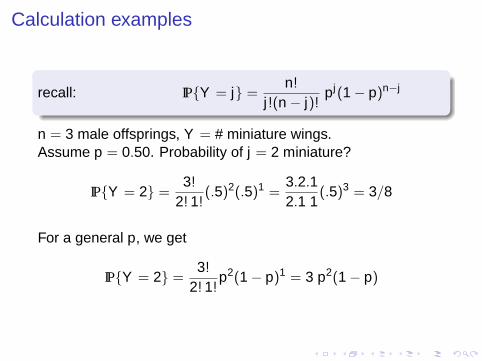
recall: IP{Y = j} =n!
j!(n − j)!pj(1− p)n−j
n = 3 male offsprings, Y = # miniature wings.Assume p = 0.50. Probability of j = 2 miniature?
IP{Y = 2} =3!
2! 1!(.5)2(.5)1 =
3.2.12.1 1
(.5)3 = 3/8
For a general p, we get
IP{Y = 2} =3!
2! 1!p2(1− p)1 = 3 p2(1− p)
Calculation examples
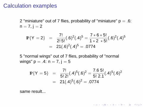
2 "miniature" out of 7 flies, probability of "miniature" p = .6:n = 7, j = 2
IP{Y = 2} =7!
2! 5!(.6)2(.4)5 =
7 ∗ 6 ∗ 5!
1 ∗ 2 ∗ 5!(.6)2(.4)5
= 21(.6)2(.4)5 = .0774
5 "normal wings" out of 7 flies, probability of "normalwings" p = .4: n = 7, j = 5
IP{Y = 5} =7!
5! 2!(.4)5(.6)2 =
7.6 5!
5! 2.1(.4)5(.6)2
= 21(.4)5(.6)2 = .0774
same result...
Calculation examples
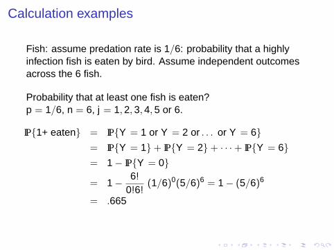
Fish: assume predation rate is 1/6: probability that a highlyinfection fish is eaten by bird. Assume independent outcomesacross the 6 fish.
Probability that at least one fish is eaten?p = 1/6, n = 6, j = 1, 2, 3, 4, 5 or 6.
IP{1+ eaten} = IP{Y = 1 or Y = 2 or . . . or Y = 6}= IP{Y = 1}+ IP{Y = 2}+ · · ·+ IP{Y = 6}= 1− IP{Y = 0}
= 1− 6!
0!6!(1/6)0(5/6)6 = 1− (5/6)6
= .665

Probability distribution
We write Y ∼ B(n, p)
B for binomial. In last example: Y ∼ B(6, 1/6). Shorthand forthis distribution table:
y 0 1 2 3 4 5 6IP{Y = y} .335 .402 .200 .054 .008 .0006 .00002
describes Y ’s probability distribution, i.e. its probability massfunction.

0 2 4 6 8 10
0.0
0.1
0.2
0.3
0.4
0.5
n= 10 , p= 0.05
Pro
babi
lity
0 2 4 6 8 100.
000.
050.
100.
150.
200.
25
n= 50 , p= 0.05
0 5 10 15 20 25
0.00
0.02
0.04
0.06
0.08
0.10
0.12
n= 200 , p= 0.05
0 5 10 15 20
0.00
0.05
0.10
0.15
0.20
0.25
n= 20 , p= 0.1
Pro
babi
lity
0 5 10 15 20
0.05
0.10
0.15
n= 20 , p= 0.5
Some Possible Values
0 5 10 15 20
0.00
0.05
0.10
0.15
0.20
0.25
n= 20 , p= 0.9

Underlying assumptions
Y ∼ B(n, p)
Trials have exactly 2 outcomes.
The probability of success p is the same for all trials.Number of trials n is fixed in advance.
If new crosses are made until some outcome is observed,then the binomial is not the correct distribution for Y .
All trials are independent.apart from the fact that they all share the same successprobability p.

Underlying assumptions
Why are assumptions not met?
Y = # kids with a cold, out of 20 in Mrs. Smith’skindergarten class
Not independent
Y = # days with snow next week
Not independent
Consider March 1, April 1, May 1, June 1, . . . , Sept 1.Y = # days with rain in Ho Chi Minh City, Vietnam, out ofthese 7 days.
unequal p’s (Monsoon ∼May-Oct)
Drug trial on 18 rats, housed 3 in a cage
Not independent
The binomial is a model , not necessarily reality.Provides structure on real world phenomena.

Underlying assumptions
Why are assumptions not met?
Y = # kids with a cold, out of 20 in Mrs. Smith’skindergarten class
Not independent
Y = # days with snow next weekNot independent
Consider March 1, April 1, May 1, June 1, . . . , Sept 1.Y = # days with rain in Ho Chi Minh City, Vietnam, out ofthese 7 days.
unequal p’s (Monsoon ∼May-Oct)
Drug trial on 18 rats, housed 3 in a cageNot independent
The binomial is a model , not necessarily reality.Provides structure on real world phenomena.

Mean and Standard deviation
If Y ∼ B(n, p) then
µ = IEY = np and σ2 = np(1− p) i.e. σ =√
np(1− p)
Recombinant fruit flies, assume genetic linkage with p = 0.2:
n = 100 fruit files. Mean: µ = 20 recombinants, standarddeviation σ =
√n ∗ .2 ∗ .8 = 4.
What would you predict: between 12 and 28recombinants? between 18 and 22?
If n = 10, 000 fruit flies: µ = 2, 000 recombinants andσ =
√10000 ∗ .2 ∗ .8 = 40 recombinants.
What would you predict: between 1,600 and 2,400recombinants? between 1900 and 2100?between 1990 and 2010?
Outline
1 The Binomial distributionProbability distributionAssumptionsMean and Standard deviation
2 The Normal DistributionIntroductionA particular case: the standard normalGeneral form
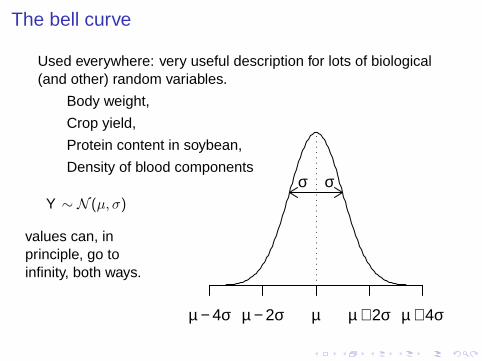
The bell curve
Used everywhere: very useful description for lots of biological(and other) random variables.
Body weight,
Crop yield,
Protein content in soybean,
Density of blood components
Y ∼ N (µ, σ)
values can, inprinciple, go toinfinity, both ways.
µ − 4σ µ − 2σ µ µ + 2σ µ + 4σ
σ σ

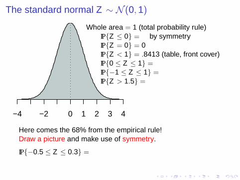
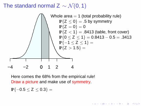
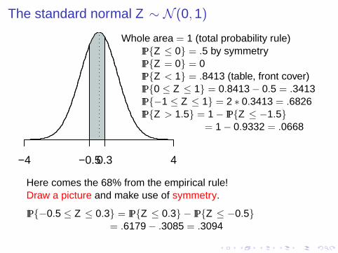
The standard normal Z ∼ N (0, 1)
−4 −2 0 1 2 3 4
Whole area = 1 (total probability rule)IP{Z ≤ 0} =
.5
by symmetryIP{Z = 0} = 0IP{Z < 1} = .8413 (table, front cover)IP{0 ≤ Z ≤ 1} =
0.8413− 0.5 = .3413
IP{−1 ≤ Z ≤ 1} =
2 ∗ 0.3413 = .6826
IP{Z > 1.5} =
1− IP{Z ≤ −1.5}= 1− 0.9332 = .0668
Here comes the 68% from the empirical rule!Draw a picture and make use of symmetry.
IP{−0.5 ≤ Z ≤ 0.3} =
IP{Z ≤ 0.3} − IP{Z ≤ −0.5}= .6179− .3085 = .3094
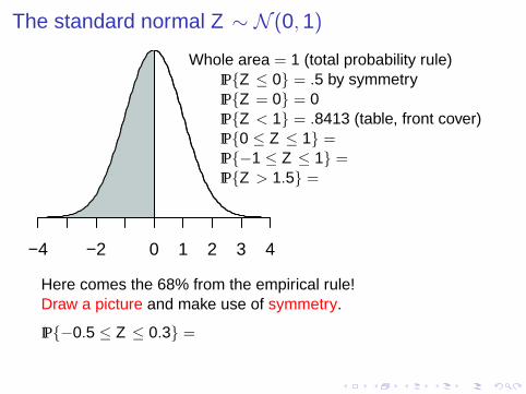
The standard normal Z ∼ N (0, 1)
−4 −2 0 1 2 3 4
Whole area = 1 (total probability rule)IP{Z ≤ 0} = .5 by symmetryIP{Z = 0} = 0IP{Z < 1} = .8413 (table, front cover)IP{0 ≤ Z ≤ 1} =
0.8413− 0.5 = .3413
IP{−1 ≤ Z ≤ 1} =
2 ∗ 0.3413 = .6826
IP{Z > 1.5} =
1− IP{Z ≤ −1.5}= 1− 0.9332 = .0668
Here comes the 68% from the empirical rule!Draw a picture and make use of symmetry.
IP{−0.5 ≤ Z ≤ 0.3} =
IP{Z ≤ 0.3} − IP{Z ≤ −0.5}= .6179− .3085 = .3094
The standard normal Z ∼ N (0, 1)
−4 −2 0 2 4−5 1
Whole area = 1 (total probability rule)IP{Z ≤ 0} = .5 by symmetryIP{Z = 0} = 0IP{Z < 1} = .8413 (table, front cover)IP{0 ≤ Z ≤ 1} =
0.8413− 0.5 = .3413
IP{−1 ≤ Z ≤ 1} =
2 ∗ 0.3413 = .6826
IP{Z > 1.5} =
1− IP{Z ≤ −1.5}= 1− 0.9332 = .0668
Here comes the 68% from the empirical rule!Draw a picture and make use of symmetry.
IP{−0.5 ≤ Z ≤ 0.3} =
IP{Z ≤ 0.3} − IP{Z ≤ −0.5}= .6179− .3085 = .3094
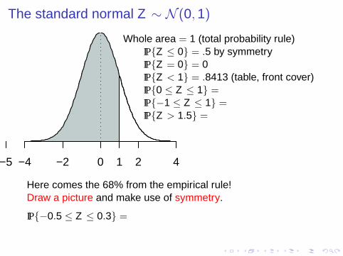
The standard normal Z ∼ N (0, 1)
−4 −2 0 2 40 1
Whole area = 1 (total probability rule)IP{Z ≤ 0} = .5 by symmetryIP{Z = 0} = 0IP{Z < 1} = .8413 (table, front cover)IP{0 ≤ Z ≤ 1} =
0.8413− 0.5 = .3413
IP{−1 ≤ Z ≤ 1} =
2 ∗ 0.3413 = .6826
IP{Z > 1.5} =
1− IP{Z ≤ −1.5}= 1− 0.9332 = .0668
Here comes the 68% from the empirical rule!Draw a picture and make use of symmetry.
IP{−0.5 ≤ Z ≤ 0.3} =
IP{Z ≤ 0.3} − IP{Z ≤ −0.5}= .6179− .3085 = .3094
The standard normal Z ∼ N (0, 1)
−4 −2 0 2 40 1
Whole area = 1 (total probability rule)IP{Z ≤ 0} = .5 by symmetryIP{Z = 0} = 0IP{Z < 1} = .8413 (table, front cover)IP{0 ≤ Z ≤ 1} = 0.8413− 0.5 = .3413IP{−1 ≤ Z ≤ 1} =
2 ∗ 0.3413 = .6826
IP{Z > 1.5} =
1− IP{Z ≤ −1.5}= 1− 0.9332 = .0668
Here comes the 68% from the empirical rule!Draw a picture and make use of symmetry.
IP{−0.5 ≤ Z ≤ 0.3} =
IP{Z ≤ 0.3} − IP{Z ≤ −0.5}= .6179− .3085 = .3094
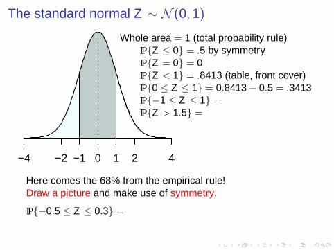
The standard normal Z ∼ N (0, 1)
−4 −2 0 2 4−1 1
Whole area = 1 (total probability rule)IP{Z ≤ 0} = .5 by symmetryIP{Z = 0} = 0IP{Z < 1} = .8413 (table, front cover)IP{0 ≤ Z ≤ 1} = 0.8413− 0.5 = .3413IP{−1 ≤ Z ≤ 1} = 2 ∗ 0.3413 = .6826IP{Z > 1.5} =
1− IP{Z ≤ −1.5}= 1− 0.9332 = .0668
Here comes the 68% from the empirical rule!Draw a picture and make use of symmetry.
IP{−0.5 ≤ Z ≤ 0.3} =
IP{Z ≤ 0.3} − IP{Z ≤ −0.5}= .6179− .3085 = .3094

The standard normal Z ∼ N (0, 1)
−4 0 41.5 5
Whole area = 1 (total probability rule)IP{Z ≤ 0} = .5 by symmetryIP{Z = 0} = 0IP{Z < 1} = .8413 (table, front cover)IP{0 ≤ Z ≤ 1} = 0.8413− 0.5 = .3413IP{−1 ≤ Z ≤ 1} = 2 ∗ 0.3413 = .6826IP{Z > 1.5} =
1− IP{Z ≤ −1.5}= 1− 0.9332 = .0668
Here comes the 68% from the empirical rule!Draw a picture and make use of symmetry.
IP{−0.5 ≤ Z ≤ 0.3} =
IP{Z ≤ 0.3} − IP{Z ≤ −0.5}= .6179− .3085 = .3094
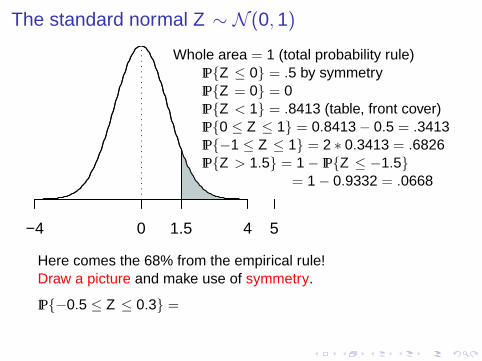
The standard normal Z ∼ N (0, 1)
−4 0 41.5 5
Whole area = 1 (total probability rule)IP{Z ≤ 0} = .5 by symmetryIP{Z = 0} = 0IP{Z < 1} = .8413 (table, front cover)IP{0 ≤ Z ≤ 1} = 0.8413− 0.5 = .3413IP{−1 ≤ Z ≤ 1} = 2 ∗ 0.3413 = .6826IP{Z > 1.5} = 1− IP{Z ≤ −1.5}
= 1− 0.9332 = .0668
Here comes the 68% from the empirical rule!Draw a picture and make use of symmetry.
IP{−0.5 ≤ Z ≤ 0.3} =
IP{Z ≤ 0.3} − IP{Z ≤ −0.5}= .6179− .3085 = .3094
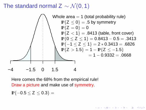
The standard normal Z ∼ N (0, 1)
−4 0 4−1.5 1.5
Whole area = 1 (total probability rule)IP{Z ≤ 0} = .5 by symmetryIP{Z = 0} = 0IP{Z < 1} = .8413 (table, front cover)IP{0 ≤ Z ≤ 1} = 0.8413− 0.5 = .3413IP{−1 ≤ Z ≤ 1} = 2 ∗ 0.3413 = .6826IP{Z > 1.5} = 1− IP{Z ≤ −1.5}
= 1− 0.9332 = .0668
Here comes the 68% from the empirical rule!Draw a picture and make use of symmetry.
IP{−0.5 ≤ Z ≤ 0.3} =
IP{Z ≤ 0.3} − IP{Z ≤ −0.5}= .6179− .3085 = .3094

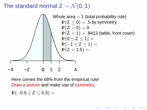
The standard normal Z ∼ N (0, 1)
−4 4−0.50.3
Whole area = 1 (total probability rule)IP{Z ≤ 0} = .5 by symmetryIP{Z = 0} = 0IP{Z < 1} = .8413 (table, front cover)IP{0 ≤ Z ≤ 1} = 0.8413− 0.5 = .3413IP{−1 ≤ Z ≤ 1} = 2 ∗ 0.3413 = .6826IP{Z > 1.5} = 1− IP{Z ≤ −1.5}
= 1− 0.9332 = .0668
Here comes the 68% from the empirical rule!Draw a picture and make use of symmetry.
IP{−0.5 ≤ Z ≤ 0.3} = IP{Z ≤ 0.3} − IP{Z ≤ −0.5}
= .6179− .3085 = .3094
The standard normal Z ∼ N (0, 1)
−4 4−0.50.3
Whole area = 1 (total probability rule)IP{Z ≤ 0} = .5 by symmetryIP{Z = 0} = 0IP{Z < 1} = .8413 (table, front cover)IP{0 ≤ Z ≤ 1} = 0.8413− 0.5 = .3413IP{−1 ≤ Z ≤ 1} = 2 ∗ 0.3413 = .6826IP{Z > 1.5} = 1− IP{Z ≤ −1.5}
= 1− 0.9332 = .0668
Here comes the 68% from the empirical rule!Draw a picture and make use of symmetry.
IP{−0.5 ≤ Z ≤ 0.3} = IP{Z ≤ 0.3} − IP{Z ≤ −0.5}= .6179− .3085 = .3094
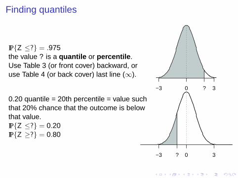
Finding quantiles
IP{Z ≤?} = .975
? = 1.96
the value ? is a quantile or percentile .Use Table 3 (or front cover) backward, oruse Table 4 (or back cover) last line (∞).
0.20 quantile = 20th percentile = value suchthat 20% chance that the outcome is belowthat value.IP{Z ≤?} = 0.20
? = −0.84
IP{Z ≥?} = 0.80
? = −0.84
−3 0 3?
−3 0 3?

Finding quantiles
IP{Z ≤?} = .975 ? = 1.96the value ? is a quantile or percentile .Use Table 3 (or front cover) backward, oruse Table 4 (or back cover) last line (∞).
0.20 quantile = 20th percentile = value suchthat 20% chance that the outcome is belowthat value.IP{Z ≤?} = 0.20 ? = −0.84IP{Z ≥?} = 0.80
? = −0.84
−3 0 3?
−3 0 3?

Finding quantiles
IP{Z ≤?} = .975 ? = 1.96the value ? is a quantile or percentile .Use Table 3 (or front cover) backward, oruse Table 4 (or back cover) last line (∞).
0.20 quantile = 20th percentile = value suchthat 20% chance that the outcome is belowthat value.IP{Z ≤?} = 0.20 ? = −0.84IP{Z ≥?} = 0.80 ? = −0.84
−3 0 3?
−3 0 3?
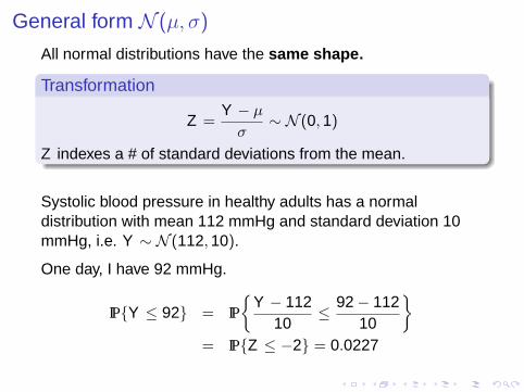
General form N (µ, σ)
All normal distributions have the same shape.
Transformation
Z =Y − µ
σ∼ N (0, 1)
Z indexes a # of standard deviations from the mean.
Systolic blood pressure in healthy adults has a normaldistribution with mean 112 mmHg and standard deviation 10mmHg, i.e. Y ∼ N (112, 10).
One day, I have 92 mmHg.
IP{Y ≤ 92} = IP
{Y − 112
10≤ 92− 112
10
}= IP{Z ≤ −2} = 0.0227

General form N (µ, σ)
µ = 112 mmHg, σ = 10 mmHg.
IP{102 ≤ Y ≤ 122} = IP
{102− 112
10≤ Y − 112
10≤ 122− 112
10
}= IP{−1 ≤ Z ≤ 1} = .6826
68.3% of healthy adults have systolic blood pressure between102 and 122 mmHg.A patient’s systolic blood pressure is 137 mmHg.
IP{Y ≥ 137} = IP
{Y − 112
10≥ 137− 112
10
}= IP{Z ≥ 2.5} = 1− .9938 = 0.0062
This patient’s blood pressure is very high...

General form N (µ, σ)µ = 112 mmHg, σ = 10 mmHg.What is “High blood pressure”? For instance, it could be thevalue BP∗ such that
IP{Y ≤ BP∗} = .95
We need z∗ such that IP{Z ≤ z∗} = .95. Table in back cover(last line): z∗ = 1.645. Thus BP∗ lies 1.645 standard deviationsabove the mean:
BP∗ = 112 + 1.645 ∗ 10 = 112 + 16.45 = 128.45 mmHg
Formal approach:
.95 = IP{Y ≤ BP∗} = IP
{Y − 112
10≤ BP∗ − 112
10
}= IP{Z ≤ z∗}
with z∗ =BP∗ − 112
10i.e. BP∗ = 112 + 10 z∗

Doing calculations with R
> pnorm(1)[1] 0.8413447> pnorm(2)-pnorm(-2)[1] 0.9544997> pnorm(3)-pnorm(-3)[1] 0.9973002> 1- pnorm(137, mean=112, sd=10)[1] 0.006209665> qnorm(.95, mean=112, sd=10)[1] 128.4485> pbinom(1, size=6, prob=1/6)[1] 0.7367755> dbinom(0:6, size=6, prob=1/6)[1] 0.335 0.402 0.201 0.054 0.008 0.001 0.000
norm normal distributionbinom binomialp probability: IP{Y ≤ . . . }q quantiled density, or probability mass
function: IP{Y = . . . }