statistical tools for analyzing measurements of...

Statistical Tools for Analyzing Measurements of Charge TransportWilliam F. Reus,† Christian A. Nijhuis,‡ Jabulani R. Barber,† Martin M. Thuo,† Simon Tricard,†

and George M. Whitesides*,†,§

†Department of Chemistry and Chemical Biology, Harvard University, 12 Oxford Street, Cambridge, Massachusetts 02138, UnitedStates‡Department of Chemistry, National University of Singapore, 3 Science Drive, Singapore 117543§Kavli Institute for Bionano Science & Technology, Harvard University, School of Engineering and Applied Sciences, Pierce Hall, 29Oxford Street, Cambridge, Massachusetts 02138, United States

*S Supporting Information

ABSTRACT: This paper applies statistical methods to analyze the large, noisy data setsproduced in measurements of tunneling current density (J) through self-assembledmonolayers (SAMs) in large-area junctions. It describes and compares the accuracy andprecision of procedures for summarizing data for individual SAMs, for comparing two ormore SAMs, and for determining the parameters of the Simmons model (β and J0). For datathat contain significant numbers of outliers (i.e., most measurements of charge transport),commonly used statistical techniquese.g., summarizing data with arithmetic mean andstandard deviation and fitting data using a linear, least-squares algorithmare prone to largeerrors. The paper recommends statistical methods that distinguish between real data andartifacts, subject to the assumption that real data (J) are independent and log-normallydistributed. Selecting a precise and accurate (conditional on these assumptions) methodyields updated values of β and J0 for charge transport across both odd and even n-alkanethiols (with 99% confidence intervals)and explains that the so-called odd−even effect (for n-alkanethiols on Ag) is largely due to a difference in J0 between odd andeven n-alkanethiols. This conclusion is provisional, in that it depends to some extent on the statistical model assumed, and theseassumptions must be tested by future experiments.

■ INTRODUCTIONUnderstanding the relationship between the atomic-levelstructure of organic matter and the rate of charge transportby tunneling across it is relevant to fields from molecularbiology to organic electronics. Self-assembled monolayers(SAMs) should, in principle, be excellent substrates for suchstudies.1 In practice, the field has proved technically andexperimentally to be very difficult (for reasons we sketch, atleast in part, in the following sections), and measurements ofrates of tunneling across SAMs have produced an abundance ofdata with often uncharacterized reliability and accuracy.Although a number of experimental factors contribute to the

difficulty of the field, there is an additional problem: namely,analysis of data. Many of the experimental systems used tomeasure tunneling across SAMs generate noisy data (in somecases, for reasons that are intrinsic to the type of measurement,because of poor experimental design or inadequate control ofexperimental variables). Regardless, with the exception of workdone using scanning probe techniques2−8 and break junctions,9

and by Lee et al.,10 the data have seldom been subjected to testsfor statistical significance, and papers have sometimes beenbased on selected data or on (perhaps) meaningful datawinnowed from large numbers of failures, without a rigorousstatistical methodology.We have worked primarily with a junction composed of three

components: (i) a “template-stripped”11 silver or gold electrode

(the “bottom” electrode)template stripping provides arelatively flat (rms roughness = 1.2 nm, over a 25 μm2 areaof Ag) surface;11 (ii) a SAM; and (iii) a top-electrode,comprising a drop of liquid eutectic GaIn alloy, with a surfacefilm of (predominantly) Ga2O3. (We abbreviate this junction as“AgTS-SR//Ga2O3/EGaIn”, following a nomenclature describedelsewhere.12−14) Figure 1 shows a schematic of an assembledjunction, including examples of defects in the substrate, SAM,and top-electrode that affect the local spacing betweenelectrodes. (The composition of the junction has beendiscussed elsewhere in detail.14) The metric for characterizingcharge transport through this junction is the current density (J,A/cm2) as a function of applied voltage (V). We calculate J bydividing the measured current by the cross-sectional area of thejunction, inferred (assuming a circular cross-section) from themeasured diameter of the contact between the Ga2O3/EGaIntop-electrode and the SAM.This paper is a part of a still-evolving effort to use statistical

tools to analyze the data generated by this junction and toidentify factors that contribute to the noise in the data. Thisanalysis is important for our own work in this area, of course. Itis alsoat least in spiritimportant in analyzing datagenerated using many SAM-based systems. We acknowledge

Received: October 31, 2011Published: February 22, 2012

Article

pubs.acs.org/JPCC

© 2012 American Chemical Society 6714 dx.doi.org/10.1021/jp210445y | J. Phys. Chem. C 2012, 116, 6714−6733

pubs.acs.org/JPCC

that our analysis contains a number of approximations. It is,however, extremely useful in identifying sources of error and inproviding the basis of future evolutions of these types ofsystems into simpler and more reliable progeny.To develop and demonstrate our analysis, we use data

collected14 across a series of n-alkanethiolate SAMs, S-(CH2)n−1CH3, for n = 9−18. Figure 2 powerfully conveys the

magnitude of the challenge faced by any analysis of chargetransport in AgTS-SR//Ga2O3/EGaIn junctions (and, westrongly suspect, other systems as well). It shows twohistograms (see the Supporting Information for details onplotting histograms) of J on a log-scale for n-alkanethiols atopposite ends of the series: the histogram of S(CH2)17CH3

(black) is superimposed on that of S(CH2)9CH3 (gray). Giventhat the lengths of these two alkanethiols differ by almost afactor of 2, the overlap between the data generated by these twoSAMs is surprisingand there are seven more compounds that

lie between these two. This overlap is not as severe when theGa2O3/EGaIn used to contact the SAM is stabilized in amicrofluidic channel15 or when a single, experienced user(rather than a group of users with different levels of experience)collects the data. Even under these favorable circumstances,however, the spread in the data is still significant. One questionthat this paper seeks to address is how to draw confidentconclusions about molecular effects when (i) the spread of thedata is comparable to the magnitude of the effect beinginvestigated and (ii) the noise in the data makes it difficult toseparate real results from artifacts.

Foundational Assumptions of Statistical Analysis ofCharge Transport through SAMs. Statistical analysisgenerally (and our analysis in particular) seeks to describepopulationsi.e., groups of items that are all related by acertain characteristic.16−18 An example of a population that westudy is the set of all possible AgTS-S(CH2)12CH3//Ga2O3/EGaIn junctions that could be prepared according to ourstandard procedure.14 Obviously, such a population isimmeasurably large, and as is typical in statistical analysis, itis impossible to measure the entire population directly. Wemust, therefore, measure a representative sample of thepopulation and then use statistical analysis to draw conclusions,from the sample, about the general population. Hence, forexample, we measure current density, J (at a particular bias, V),for a certain sample of AgTS-S(CH2)12CH3//Ga2O3 junctionsand make generalizations about J for the population of all AgTS-S(CH2)12CH3//Ga2O3/EGaIn junctions.To draw conclusions, from a random sample, about the

population from which it is derived, it is necessary to have astatistical model that identifies the meaningful parameters ofthe population and describes how the observations in a samplecan be used to estimate those parameters. We currently use astatistical model to describe how values of J arise from apopulation of AgTS-SR//Ga2O3/EGaIn junctions. Our model isa statistical extension of the approximate but widely usedSimmons model19 (eq 1), which describes tunneling throughan insulator, at a constant applied bias; the issues raised in theanalysis would, however, apply as well to other models.

= −βJ J e d0 (1)

Figure 1. Formation and structure of a AgTS-SR//Ga2O3/EGaIn junction. To form the junction, a conical tip of Ga2O3/EGaIn, suspended from asyringe, is lowered into contact with a SAM on a AgTS substrate. The substrate is grounded; an electrometer applies a voltage to the syringe andmeasures the current flowing through the junction. The schematic representation of the junction shows defects in the AgTS substrate and SAM, aswell as adsorbed organic contaminants, and roughness at the surface of the Ga2O3 layer. Note that some of these defects produce “thick” areas, whileothers produce “thin” areas.

Figure 2. Histograms of log|J/(A/cm2)|, at V = −0.5 V, for SAMs oftwo n-alkanethiols: S(CH2)17CH3 (gray bars) and S(CH2)9CH3 (blackbars). These histograms overlap to a significant degree, despite beingon opposite ends of the series of n-alkanethiols. In other words, thedispersion (spread) in the data for these two SAMs (which arerepresentative of other n-alkanethiols) is similar to the effect ofchanging n from 10 to 18.

The Journal of Physical Chemistry C Article

dx.doi.org/10.1021/jp210445y | J. Phys. Chem. C 2012, 116, 6714−67336715

In eq 1, d is the molecular length (either in Å or number ofcarbon atoms); J0 is a (bias-dependent) pre-exponential factorthat accounts for the interfaces between the SAM and theelectrodes; and β is the tunneling decay constant. TheSimmons model predicts only individual values of J through ajunction of known, and constant, thickness. It is not, therefore,a statistical modelone that predicts the properties of arandom sample comprising measurements of many junctions.To develop a statistical model, we began with the assumption

that the junctions we fabricate fall into two categories: (i)junctions in which, despite the presence of defects, the basicAgTS-SR//Ga2O3/EGaIn structure dominates charge transport,in keeping with the Simmons model, and (ii) junctions inwhich experimental artifacts alter the basic structure of thejunction to something radically different from AgTS-SR//Ga2O3/EGaIne.g., penetration of the SAM by the Ga2O3/EGaIn electrode yields a junction of the form AgTS//Ga2O3/EGaInand invalidate the Simmons model as a description ofcharge transport. The first type of junctions give data that are“informative” about charge transport, while the second typegive data that are difficult to interpret, within the framework ofthe Simmons model, and thus “noninformative”. The goal ofour statistical analysis, therefore, is to characterize data that areinformative and ignore data that are noninformative, by usingsome method to discriminate between the two.There are two major ways to draw a distinction between

informative and noninformative data: (i) construct a parametricstatistical model16−18 that assumes that informative data followa certain probability distribution, while noninformative datafollow a different distribution, or (ii) assume that the majorityof the data are informative and choose a methodology that isinsensitive to relatively small numbers of extreme data (that is,a “robust” method20,21) since these data are likely to benoninformative. In this paper, we discuss techniques that followeach of these approaches and argue that they are superior toother, more common techniques (which we also discuss) thatdo not distinguish between informative and noninformativedata.Introduction to Our Parametric Statistical Model for

Measurements of Charge Transport. In constructing ourparametric statistical model, we used the Simmons model19 as astarting point. We assumed that β and J0 are constants and thatthe actual values of d in informative AgTS-SR//Ga2O3/EGaInjunctions vary according to a normal distribution (Figure 3A;see Supporting Information and ref 16 for a discussion ofstatistical distributions), as a result of noncatastrophic defects22

in the AgTS substrate, the SAM, and the Ga2O3/EGaInelectrode.23 When the Simmons model holds, J dependsexponentially on d, so a normal distribution of d wouldtranslate to a log-normal distribution of J (i.e., a normaldistribution of log|J/(A/cm2)|; hereafter, log|J| for conven-ience). In other words, our model predicts that informativemeasurements of log|J| are normally distributed. On the basis ofthis assumption, our statistical model predicts that log|J| for anypopulation of AgTS-SR//Ga2O3/EGaIn junctions will have twocomponents: (i) a normally distributed component that isinformative and (ii) a component comprising noninformativevalues of log|J| that follow an unknown and unspecifieddistribution. Aside from having some a priori physicaljustification, these two components predicted by our statisticalmodel are observed in experimental results (an examplelog|J|for S(CH2)17CH3is shown in Figure 3; these data have beenpublished previously14). In all cases, a prominent, approx-

imately Gaussian peak16 is easily identifiable, but anomalies(Figure 3B) are also present: (i) long tails (portions of data thatextend beyond the Gaussian peak, to the left or right, and causethe peak to be asymmetric) and (ii) outliers (individual data, orclusters of data, that are separated from the main peak of thehistogram by regions of “white space”).20,24 The differencebetween these two categories is somewhat subjective andarbitrary, and we present them only as guides to aid the readerin visualizing the pathologies of distributions of log|J|. None ofthe methods of analysis described in this paper requiredistinguishing between long tails and outliers; we, therefore,refer to them collectively as “deviations of log|J| fromnormality”.

Figure 3. Deviations of log|J| from normality and their effects onMethods 1−3. (A) The standard normal distribution, with a mean of 0and a standard deviation of 1 (these quantities are unitless). (B) Thefirst of two identical histograms of log|J(−0.5 V)/(A/cm2)| forS(CH2)17CH3. This plot shows two primary deviations of log|J| fromnormality: (i) a long tail (i.e., a larger share of the sample to the rightof the peak than in a normal distribution), and (ii) outliers (data thatlie far from the peak). (C) Methods 1−3 respond differently to thesedeviations of log|J| from normality, as shown by their estimates for thelocation of the sample. Method 1 responds the least to the long tailand outliers on the right. Method 2 responds moderately to them, andMethod 3 responds strongly to them.



A key implication of our statistical model is that the normallydistributed component of log|J| is the only component thatgives meaningful information about the SAM. According to themodel, deviations of log|J| from normality arise from processesthat dramatically alter the typical structure of the junction andmay mislead a naive analysis that treats these deviations asinformative. If the model is correct, the analysis of log|J| should,therefore, be designed to ignore any deviations of log|J| fromnormality.We believe that this model offers a reasonably accurate

description of log|J| (we offer further justification for our modelin the Experimental Design section), but we recognize that ourmodel could be wrong in an important way. Specifically, if thecomponent of log|J| arising from the typical behavior of thejunction follows something other than a normal distribution(i.e., if d is not normally distributed or if β or J0 variessignificantly between junctions), then, by definition, eveninformative measurements of log|J| should deviate fromnormality, probably to a small extent.If our statistical model is wrong in this way, then ignoring

deviations of log|J| from normality will lead to similarly small,but possibly significant, errors. On the other hand, an approachthat incorrectly treats all data as informative will be prone tolarge errors from the influence of extreme data. Between thesetwo approaches would lie methods that neither assume that log|J| is normal nor respond strongly to extreme values. Each of themethods of statistical analysis discussed in this paper (Figure 4)falls into one of these three categories, according to howstrongly they respond to deviations of log|J| from normality.The relative accuracy of these different methods of analysis willdepend on whether our statistical model is eventuallyconfirmed or discredited.Also, the precision (but not the accuracy) of all of the

methods of analysis described in this paper depends on theassumption that our measurements of log|J| are independentand uncorrelated to one another. We are relatively certain thatthis assumption is wrong (for instance, values of log|J| measuredwithin the same junction correlate more with one another thanvalues of log|J| measured from two different junctions), and wediscuss, in the Results and Discussion section, a procedure to

correct for violations of this assumption. If this correction isinsufficient, then all methods of analysis will overstate thestatistical confidence of their conclusions and underestimate thewidths of confidence intervals (see Results and Discussion).Further research is needed to determine to what extentmeasurements of log|J| are correlated and how strong of acorrection must be applied to account for this correlation.

Comparison of Methods for Analyzing Charge Trans-port. We are interested in two categories of statistical results:(i) single-compound statistics, which summarize measurements ofcharge transport through a single type of SAM (i.e., a particularcompound) and enable comparisons between two SAMs, and(ii) trend statistics, which lead to conclusions about thedependence of charge transport on some parameter (such asmolecular length) that varies across a series of SAMs. In thispaper, we describe five methods of analyzing charge transport.Figure 4 schematically shows that Methods 1−3 begin bycalculating single-compound statistics and then use thoseresults to determine trend statistics, while Methods 4a and 4bdo not produce single-compound statistics and instead proceeddirectly from the data (samples of log|J|) to calculation of trendstatistics. It is not necessary to choose only one method ofanalysis for both single-molecule and trend statistics; in fact, weshall show that, in some cases, it is best to use one method toestimate single-compound statistics and another to estimatetrend statistics.

Single-Compound Statistics. Methods 1−3 generate single-compound statistics that describe samples of log|J| for SAMs ofa particular compound. Each method has a procedure forcalculating (i) the location (sometimes called the center, orcentral tendency) of the sample, (ii) the dispersion (sometimescalled the scale, or spread) of the sample, and (iii) a conf idenceinterval that surrounds the location and has a width related tothe dispersion and the number of data in the sample.16−18,20 Toestimate the location and dispersion, respectively, Method 1uses the mean (μG) and standard deviation (σG) determined byfitting a Gaussian function to the sample of log|J|; Method 2uses the median (m) and adjusted median absolute deviation(σM) or interquartile range of the sample; and Method 3 usesthe arithmetic mean (μA) and standard deviation (σA) of the

Figure 4. Schematic of the four methods of analyzing charge transport discussed in this paper. Methods 1−3 use the data (samples of log|J|) tocalculate single-compound statistics; plotting those statistics, and fitting the plots, yields trend statistics. For Method 1, μG is the Gaussian mean; forMethod 2, m is the median; and for Method 3, μA is the arithmetic mean. Methods 4a and 4b proceed directly to plotting and fitting the raw data todetermine trend statistics. The bottom row gives the sensitivity of each method to common deviations of log|J| from normality (long tails andoutliers).



sample. (These quantities, and the procedures used by eachmethod for calculating confidence intervals, are detailed in theResults and Discussion section.)Each method makes different assumptions about the

distribution of log|J|. Method 1 employs an algorithm thatessentially “selects” the most prominent peak in the sample oflog|J| and disregards the rest. In other words, Method 1 closelyfollows the statistical model described above, in that it assumesthat deviations of log|J| from normality (i.e., long tails oroutliers; see Figure 3B) are not informative about chargetransport through the SAM and ignores them. Theappropriateness of Method 1 for statistical analysis depends,therefore, on the correctness of this assumption. Methods 2 and3 both depart from the statistical model by taking into account,to different degrees, deviations of log|J| from normality. Method2 (m and σM) responds only moderately to such deviations,while even a few extreme data can have a significant effect onMethod 3 (μA and σA).Figure 3C briefly demonstrates the different responses to

deviations of log|J| from normality of the locations estimated bythese three methods. The histogram of S(CH2)17CH3 exhibits along tail to the right (toward high values of log|J|). This tailstrongly influences the arithmetic mean (Method 3) and “pulls”it to the right by 0.23 log-units, in comparison with theGaussian mean (Method 1). By comparison, the median(Method 2) is only moderately affected by the tail and differsfrom the Gaussian mean by 0.06 log-units. Although even thedivergence between Methods 1 and 3 may not appearsignificant, there are two reasons to take it seriously. (i) Forthe two n-alkanethiols on the extreme ends of the series,S(CH2)8CH3 and S(CH2)17CH3, the locations of thedistributions of log|J| only differ by about 3.0−3.5 log-units(depending on the method used to estimate the locations). Thedivergence, evident in Figure 3, between Method 1 and Method3, therefore, represents approximately 8% of the total change inlog|J| across the entire series of n-alkanethiols. When comparingtwo adjacent n-alkanethiols (e.g., n = 17 and 18), thedifferences between Methods 1−3 will be even moresignificant. (ii) The data discussed in this paperin particular,n-alkanethiols for which n is evenwere collected byexperienced users and probably exhibit fewer deviations fromnormality than would data collected by inexperienced users.For inexperienced users, then, the effect of outliers and tails onMethod 3 may be large, and using Method 1 or 2 is importantto draw accurate conclusions from the data.The goal of single-compound statistics is to estimate the

location (and, secondarily, the dispersion) of the population ina way that is both precise and accurate. The precision of theestimated location is determined by the width of the confidenceinterval, such that a narrow confidence interval indicates aprecise (although not necessarily accurate) estimate.16 Theaccuracy of the location estimated by a given method dependson how well the assumptions of the method conform to reality.If, through its assumptions, a method correctly discriminatesbetween informative and noninformative data, then its estimatefor the location will generally be accurate, in the sense that thetrue location of the log|J| for the population will, with a statedconfidence (e.g., 99%), lie within the confidence interval.17 Ifthe method makes incorrect assumptions about the data, thenthe confidence interval cannot be trusted to contain, at thestated level of confidence, the true location of the population.Because we believe that our statistical model comprisesreasonably correct assumptions about the data, we recommend

the use of either Method 1 (Gaussian mean) or 2 (median), butnot Method 3 (arithmetic mean), for estimating single-compound statistics.

Trend Statistics. When calculating trend statistics, such as βand J0 (see eq 1), it is possible to use any of the four methodsdiscussed in this paper. In general, the process of calculatingtrend statistics involves plotting log|J|, measured across a seriesof compounds, against some molecular characteristic that variesacross the series (e.g., molecular length, n) and then fitting theplot to a model that specifies the relationship between thedesired trend statistics and the data. The plotted values of log|J|are either single-compound statistics summarizing log|J| foreach molecule (Methods 1−3) or the raw data themselves; thatis, all measured values of log|J| (Methods 4a and 4b).All methods use an algorithm to fit (values summarizing) log|

J| vs n to a linear model (the Simmons model predicts a linearrelationship between log|J| and n, via the parameter d). Thechoice of the fitting algorithm determines the influence exertedon the outcome by data that lie far from the fitted line (thesedata are roughly equivalent to those that cause log|J| to deviatefrom normalityi.e., long tails and outliers in each sample).For Methods 1−3, the choice of the fitting algorithm has littleeffect on the outcome because, in the process of estimatingsingle-compound statistics, each Method has already made theassumptions that determine how it responds to extreme data.By summarizing log|J| for each compound and passing thosesummaries to the fitting algorithm that determines trendstatistics, these Methods have compressed the wealth ofinformation in each sample and essentially ensured that thefitting algorithm will not “see” any extreme data. In calculatingtrend statistics, therefore, Methods 1−3 carry forward all of therespective assumptions and biases that they exercise in thecalculation of single-compound statistics.For Methods 4a and 4b, by contrast, the choice of the fitting

algorithm has a (potentially) large impact on the resultsbecause deviations from normality are invariably present in theraw data. Method 4a uses an algorithm that minimizes the sumof the absolute values of the errors between the data and thefitted line (a “least-absolute-errors algorithm”), while Method4b employs an algorithm that minimizes the sum of the squaresof those errors (a “least-squares algorithm”). Method 4aresponds to deviations of log|J| from normality in a manneranalogous to that of Method 2; both methods are onlymoderately affected by such deviations. Method 4b, on theother hand, is analogous to Method 3, in that it respondsstrongly to deviations from normality.Although Methods 4a and 4b cannot give single-compound

statistics, they have the advantage of offering far greaterprecision than Methods 1−3 in estimating trend statistics.Because Method 4a has assumptions similar to Method 2, theaccuracies of the two methods will also be similar (by the sametoken, the accuracy of Method 4b will be similar to that ofMethod 3). We, therefore, recommend using either Method 1(fitting Gaussian means of log|J| with a least-squares algorithm)or Method 4a (fitting all values of log|J| with a least-absolute-errors algorithm) to estimate trend statistics. If estimatesproduced by these two methods agree, then it may bepreferable to use Method 4a because of its high precision.Figure 4 schematically depicts how each of the four methods

progresses from histograms of log|J| for single compounds(three compounds are shown, but each method can involve anarbitrary number) to analysis of the trend across thosecompounds; the figure also indicates the type of information



given by each of the four methods. All four methods responddifferently to deviations of log|J| from normality, and as we shalldemonstrate, the choice of method can affect the conclusionsabout charge transport drawn by the analysis.

■ BACKGROUNDMethods for Measuring Charge Transport. Many

approaches exist for measuring charge transport through self-assembled monolayers (SAMs) of thiol-terminated molecules.These approaches can be segregated into those that producesmall-area (from single-molecule to ∼100 nm2) junctionscomprising relatively few molecules (scanning probe techni-ques2−8 and break junctions9) and those that produce large-area (>1 μm2) junctions.Most large-area junctions employ a SAM, supported on a

conductive substrate and contacted by a top-electrodeeithera layer of evaporated Au, a drop of liquid Hg supporting a SAM(Hg-SAM), or a structure of Ga2O3/EGaIn. While it wascommon, in the past, to evaporate Au directly onto the SAM,25

this procedure resulted in low yields (up to 5% when executedvery carefully but usually <1%)10 of nonshorting junctions andis now known to damage the SAM.26 Most currently successfullarge-area junctions employ a top-electrode with an insulatingor semiconducting barrier (a “protective layer”) between themetal and the SAM to protect against damage from high-energymetal atoms (during evaporation) and guard against metalfilaments formed by the electromigration of metal atomsthrough defects in the SAM. Examples of protective layersbetween the SAM and the metal of the top-electrode includeconducting polymers (e.g., Au-SAM//PEDOT:PSS/Au junc-tions of Akkerman et al.27 and Au-SAM//(polymer)/Hg dropjunctions of Rampi et al.28), a second SAM (e.g., Ag-SAM//SAM-Hg junctions of us22,29 and others30−32), and a layer ofmetal oxides (e.g., our AgTS-SAM//Ga2O3/EGaIn junc-tions12,14).There are two exceptions to the rule of the protective layer in

large-area junctions. (i) Cahen et al.33−35 use n-Si-R//Hg andp-Si-R//Hg junctions, in which a layer of alkenes, covalentlyattached to a doped and hydrogen-passivated Si surface, isdirectly contacted by a drop of Hg. Use of a semiconducting,rather than a metallic, substrate reduces the migration of metalatoms responsible for metal filaments and shorts. (ii) Lee etal.10 continue to evaporate Au directly on the SAM to form Au-SAM//Au junctions. Skilled users can generate yields of 1−5%,and the authors use careful statistical analysis to distinguishbetween real data and artifacts resulting from SAMs damagedby the direct evaporation of Au.AgTS-SAM//Ga2O3/EGaIn Junctions. In our nomenclature,

AgTS denotes an ultraflat Ag substrate produced by templatestripping,11 while Ga2O3/EGaIn denotes the eutectic alloy ofgallium and indium (75% Ga, 25% In by weight, mp = 15.5 °C)with its surface layer of oxide.36 The rheological properties ofthis composite material make it possible to mold it into conicalshapes but still allow it to deform under applied pressure. Theseproperties make Ga2O3/EGaIn an excellent material forforming soft, microscale contacts to structures like SAMs.The questiondoes Ga2O3/EGaIn form good electrical

contact to SAMs?hinges on the resistivity of the Ga2O3surface film. We have measured37 the thickness (∼0.7 nm is theaverage thickness, although some regions may be severalmicrometers thick), composition (primarily Ga2O3), andresistivity (105−106 Ω·cm) of the film. The film of Ga2O3,like all surfaces in the laboratory, supports a layer of adsorbed

organic material, which is undoubtedly present in AgTS-SAM//Ga2O3/EGaIn junctions (and in many other junctions). Themeasured thickness of this layer is ∼1 nm,36,37 and itscomposition probably depends on the environment; however,it is probably a discontinuous layer, rather than a continuoussheet.38 We measured the resistivity of the Ga2O3 film, with itsadsorbed organic layer, using two direct methods13 (contactingstructures of Ga2O3/EGaIn with Cu and ITO electrodes) andone indirect method (placing an upper bound on the resistivityof the Ga2O3 using the value of J0, explained below, for n-alkanethiols). All three methods converge to a range of 105−106Ω·cm for the resistivity of the Ga2O3 film. This range is at least3 orders of magnitude lower than the resistivity of a SAM ofS(CH2)9CH3 (∼109 Ω·cm), the least resistive SAM that wehave measured.39 The Ga2O3 film, and especially the layer ofadsorbed organic matter on its surface, is certainly the leastunderstood component of our system. On the basis of thesemeasurements, however, we conclude that the Ga2O3 film, withits adsorbed organic layer, is sufficiently conductive that it doesnot affect the electrical characteristics of the junction. Thisconclusion is supported by our recent study40 that usesmolecular rectification in various SAMs to show that the SAM,rather than the Ga2O3 layer, dominates charge transportthrough the junction.

Tunneling through SAMs. As stated in the introduction toour statistical model, tunneling through SAMs is widelyassumed to follow eq 1.19 Typically, one of the first experimentsperformed with any experimental system is to measure log|J|through SAMs of a series of n-alkanethiols of increasingmolecular lengths (d) and to calculate the values of β and J0.The tunneling decay constant, β, is related to the height andshape of the tunneling barrier posed by the SAM. Because thevalue of β theoretically depends only on the molecular orbitalsof the SAM, and not on the interfaces between the SAM andthe electrodes, β is expected to be largely independent of themethod used to measure log|J| and is, thus, a useful standardwith which to validate new techniques. By contrast, J0 is a pre-exponential factor that accounts for factors that contribute to“contact resistance”the resistivity and density of states of theelectrodes and any tunneling barriers at the interfaces betweenthe SAM and the electrodes. While it is rare to find a value of J0in the literature, this parameter also contains importantinformation about the electrodes and interfaces in ajunctioninformation that is complementary to that conveyedby β. Thus, J0 could be used to compare different techniques formeasuring charge transport through SAMs.The Simmons model contains many assumptions (it is, after

all, a simplification of a model originally designed to describetunneling through a uniform insulator with extendedconduction and valence bands), the most significant of whichis that tunneling is the only operative mechanism of chargetransport through the SAM.19 Another significant assumption isthat the complicated tunneling barrier posed by a particularclass of SAMs can be described by a simplified “effective”barrier of a certain height and that this height does not varywith the length of the molecules in the SAM (i.e., that β doesnot depend on d). Despite these assumptions, eq 1 showsreasonable agreement with results for n-alkanethiols in theapproximate range of n = 8−20, with values of β of 0.8−0.9 Å−1

(1.0−1.1 nC−1),41 and it is now standard practice to report the

value of β for n-alkanethiols as one (often the primary, or only)parameter of interest.



Defects in SAM-Based Junctions Necessitate Report-ing of All Data. Measurements of charge transport throughSAMs have often neglected the contribution of (probably)unavoidable variations in the system to the dispersion of data.Because J depends exponentially on the thickness of the SAM, Jcan be extremely sensitive to defects in a tunneling junction,especially those that decrease the local distance betweenelectrodes (so-called “thin-area” defects).22 For example,assuming a value of 0.8 Å−1 for β, a defect 5 Å thinner thanthe nominal thickness of the SAM would carry a current densitymore than 50 times that of a corresponding area on a defect-free SAM. If such “thin” defects comprised just 2% of the totalarea of the junction, then the same amount of current wouldpass through those thin-area defects as through the rest of the(defect-free) SAM. As a result of the exponential dependence ofJ(V) on d and β, thin-area defects can easily dominate chargetransport through the junction. By contrast, thick-area defects(those that increase the local separation between electrodes)can usually be ignored because their contribution to J(V) issmall relative to other sources of error. Many types of defectsare common in both the AgTS substrate (e.g., grain boundaries,vacancy islands, and step edges) and the SAM (e.g., domainboundaries, pinholes, disordered regions, and physisorbedcontaminants).22

These defects presumably give rise to the large spreadobserved in distributions of log|J|. The roughness of the metalsubstrate (whether Au or Ag) is one of the most significantfactors in determining the density of defects in SAM-basedjunctions. In a previous paper,11 we showed that usingtemplate-stripped substrates results in smoother surfaces (forAgTS, rms roughness = 1.2 nm over a 25 μm2 area) than usingsurfaces as-deposited by electron-beam evaporation (for as-deposited Ag, rms roughness = 5.1 nm over a 25 μm2 area). InAg-SAM//SAM-Hg junctions, this decrease in roughnessbetween as-deposited and template-stripped Ag decreased therange of measured values of J by several orders of magnitudeand increased the yield of working junctions by more than afactor of 3.22

■ EXPERIMENTAL DESIGN“Informative” vs “Noninformative” Measurements of

log|J|. The Simmons model19 (eq 1) of tunneling predictsindividual values of J for known values of d but does notdescribe actual measurements of J (or log|J|). Actual measure-ments comprise random samples of many junctions, acrosswhich the parameters of the Simmons model (most likely d, butpossibly β and J0) certainly vary. Because the Simmons modeldoes not specify how real data arise from random sampling ofcharge transport (i.e., it is not a statistical model), our statisticalanalysis must account for what the Simmons model ignores, toderive meaningful results from measurements of log|J|.We begin by recognizing that, in our junctions (and SAM-

based junctions in general), there are two classes of defects: (i)defects that preserve the basic AgTS-SR//Ga2O3/EGaInstructure of the junction, even while changing d, and (ii)defects (perhaps better termed “artifacts”) that disrupt the basicstructure of the junction. Defects belonging to the first classmight include, for example, domain boundaries, pinholes,disordered regions, and physisorbed contaminants on the SAM.Even though this class of defects may alter d in a junction, theSimmons model remains a valid description of charge transportthrough the junction because charge must still tunnel betweenthe AgTS and Ga2O3/EGaIn electrodes, through the SAM. In

the second class of defects belong artifacts, such as areas inwhich the Ga2O3/EGaIn electrode penetrates or intrudes intothe SAM, regions of bare EGaIn (lacking a Ga2O3 film) incontact with the SAM, and metal filaments that bridge the twoelectrodes and bypass the SAM. These artifacts not only changed in the junction but also change (at least) J0 and might alterthe mechanism of charge transport between electrodes to someprocess other than tunneling. In short, these types of artifactsinvalidate the Simmons model (with its assumption of aconstant J0 for AgTS-SR//Ga2O3/EGaIn junctions with aconstant R group) as a description of charge transport throughthe junction.There is nothing particularly controversial in partitioning

defects into those that preserve the integrity of the Simmonsmodel and those that destroy it nor in stating that the formerresult in measurements that are informative about chargetransport through the SAM, while the latter result inmeasurements that are noninformative. The question is howto account fully for the informative data while minimizing theeffect of noninformative data on the analysis. There are,broadly, two ways to approach this question: (i) to use aparametric (or semiparametric) statistical model16,17 thatdifferentiates between the distributions of informative andnoninformative data to identify the former and discard thelatter and (ii) to assume that informative data predominate overnoninformative data and use an analysis that responds stronglyto the bulk of the data (no matter how the data are distributed)and weakly to a small number of extreme values.20,21 As we willshow, Method 1 follows the first approach, while Method 2(and Method 4a) follows the second approach. (Methods 3 and4b follow another, inferior, approach that does not discriminatebetween informative and noninformative data; we include themin this paper to illustrate their deficiencies because they are,unfortunately, the methods most commonly used outside ofstatistical disciplines.)

Method 1 Uses a Statistical Model to Distinguishbetween Informative and Noninformative Data. Method1 depends on a statistical model that predicts that when log|J|arises from informative measurements those data are normallydistributed. The statistical model is based on the followingreasoning: when the Simmons model holds, the statisticaldistribution of log|J| is determined by the distributions of J0, β,and dif one knows the distributions of these threeparameters, one can predict the distribution of log|J| thatresults from informative measurements. Our statistical modelassumes that, in junctions that generate informative data, d isnormally distributed, while J0 and β are approximately constant(i.e., if they vary, their contributions to the dispersion of log|J|are negligible, compared to the contribution of d).42 Since log|J|is proportional to d, if d is normally distributed, then log|J| isalso normally distributed. Method 1 follows this statisticalmodel by employing a fitting algorithm to “seek out” the largestcomponent of the histogram of log|J| that conforms to a normaldistribution and “ignore” the rest. If the model is correct, thenMethod 1 finds the informative data in the most prominentGaussian peak in the sample and rejects the noninformativedata that deviate from this peak.There are two lines of reasoning that support the

assumptions that log|J| is normally distributed. (i) That d isnormally distributed is probable because normal distributionsarise frequently in nature when a variable is influenced by manyuncorrelated factors.18 If the factors that determine the densityand type of defects in a junction, therefore, are many and



uncorrelated with one anothera plausible scenariothen dwill be normally distributed, as will log|J|. (ii) Previousexperiments by us12,14 (and others10), such as the data shownin Figure 3B, are consistent with log|J| being approximatelynormally distributed. Although histograms of log|J| are oftennoisy and slightly asymmetric, there is almost always aprominent peak resembling a Gaussian function identifiablein every histogram.Despite some theoretical and experimental support, the

assumption that log|J| is normally distributed might still bewrong. Other distributions, such as a Cauchy distribution(sometimes called a Lorentzian distribution) or a Student’s t-distribution, may also be consistent with observed histogramsof log|J|, and we cannot entirely rule them out; however, theylack the a priori physical justification of a normal distribution. Itis, however, plausible that while d is normally distributed ourprocedure for measuring log|J| does not randomly sample d, butthat there is some correlation in the values of d for junctionsmeasured under similar conditions. For example, the junctionsformed on a common AgTS substrate (supporting a SAM) mayhave values of d that cluster around a certain value (e.g., 10 Å),whereas the values of d for junctions formed on a different AgTS

substrate may cluster around a higher value (e.g., 12 Å),perhaps due to differences in the amount of organiccontaminants present in the environment. In such a case, thefirst AgTS substrate would result in one normal distribution oflog|J|, while the second substrate would result in another,overlapping normal distribution, centered at lower values of log|J| than the first.Such clustering may exist at multiple levels, such as between

AgTS substrates, Ga2O3/EGaIn electrodes, operators, or timesof year during which measurements were performed.Investigating the individual contributions of each level toclustering in log|J| (via clustering in d), and answering thequestion of whether such clustering is significant enough tocause log|J| to deviate noticeably from normality, would entailan in-depth experimental study that is beyond the scope of thispaper. We do not know whether clustering violates theassumption that log|J| is normally distributed, but we raise itas a concern, to disclose a potential failure of our statisticalmodel and to motivate the development of multiple methods ofstatistical analysis to respond flexibly to such a contingency.Clustering would possibly affect the accuracy of Method 1,

but it would also possibly affect the precision of all of themethods described in this paper, as expressed by the widths ofthe confidence intervals around parameters estimated by eachmethod. As explained in the Results and Discussion section, thewidth of a confidence interval decreases as the number of dataincreases; that is, many measurements lead to a narrowconfidence interval. For each of Methods 1−4, this relationshipbetween the width of a confidence interval and the number ofdata depends on the assumption that the data are independentfrom, and uncorrelated to, one another. If there is significantclustering of measurements of log|J|, then this assumption willbe violated, the widths of confidence intervals underestimated,and the precision of results overstated. In the Results andDiscussion section, we discuss a procedure for estimating thecorrelation within a sample (termed “autocorrelation”) andcorrecting for its effect on the width of confidence intervals. Wedo not currently have enough information to evaluate whetheror not this procedure adequately corrects for autocorrelation,and we emphasize the need for further experiments to

investigate and minimize the amount of autocorrelation inour measurements.

Methods 2 and 4a Do Not Assume a SpecificDistribution for log|J| but Avoid Extreme Values.Currently, we are reasonably confident that our statisticalmodel describes real measurements of log|J| with enoughaccuracy to be useful, and we, therefore, favor Method 1 in ouranalysis. In case future experiments or insights cast doubt onour statistical model, we offer Method 2 as a substitute thatdoes not depend on our model but does an adequate job ofminimizing the effect of (probably) noninformative measure-ments on the analysis. Method 2 uses the median and otherquantiles to characterize log|J|. Since well-defined quantiles existfor every continuous probability distribution, Method 2 doesnot require that log|J| be normally distributed.16 The mediantends to follow the bulk of the data in a sample, and it is muchless influenced by extreme values than the mean.20 Ifinformative measurements constitute the bulk of the data,therefore, then even extreme values resulting from non-informative measurements will have a relatively small effecton Method 2. Method 4a, as we will show below, carries thesame relative insensitivity21 to extreme values as Method 2.Methods 3 and 4b, by contrast, are relatively sensitive toextreme values20 and are likely to allow noninformativemeasurements to bias the conclusions of statistical analysis.

■ RESULTS AND DISCUSSIONOverview of Assembly of AgTS-S(CH2)9CH3//Ga2O3/

EGaIn Junctions and Measurement of Charge Transport.We have previously published a large data set comprising log|J|for n-alkanethiols (n = 9−18), with both odd and even numbersof carbon atoms in the backbone.14 We elected to use this dataset, to test and demonstrate the analytical methods described inthis paper, for two reasons: (i) because the series of even-numbered alkanethiols (n = 10, 12, 14, 16, 18) is the standarddata set used to calibrate and compare experimental techniquesfor measuring charge transport through SAMs and (ii) becausethe series of both odd and even alkanethiols (n = 9−18) showsa subtle effect (the “odd−even” effect) that cannot beaccurately characterized without careful statistical analysis.In our previous publication,14 we formed SAMs of

S(CH2)9CH3 (decanethiol) on template-stripped silver (AgTS)substrates and made electrical contact to these SAMs usingcone-shaped microelectrodes of the liquid eutectic of galliumand indium (75% Ga, 25% In by weight, with a surface ofpredominantly Ga2O3). We denote the resulting structure a“AgTS-S(CH2)9CH3//Ga2O3/EGaIn junction”; detailed proce-dures for forming SAMs on AgTS, fabricating cone-shapedelectrodes of Ga2O3/EGaIn, and assembling these junctionshave been given elsewhere.13,14 After forming a junction, wegrounded the AgTS substrate and applied a voltage (V) to theGa2O3/EGaIn electrode while measuring the current flowingbetween the two electrodes. We applied the voltage in steps of50 mV, with a delay of 0.2 s between steps, starting at 0 V,increasing to +0.5 V, decreasing to −0.5, and returning to 0 V; acycle, beginning and ending at 0 V, constituted one J(V) trace.We calculated the current density (J) by dividing the currentthrough the junction by its estimated contact area, which wedetermined by measuring the diameter of the junction andassuming a circular contact between the Ga2O3 electrode andthe SAM.

Excluding Shorts Prior to Analysis. Some analytical toolsare especially sensitive to outliers in distributions of log|J|, so it



is best to begin by excluding any data that are unambiguouslyknown to be artifacts, as long as there is a simple procedure fordoing so. For one type of artifactshort circuits or simply“shorts”there is such a procedure. We define shorts as valuesof current that reach the compliance limit of our electrometer(±0.105 A); given the range of contact areas for our junctions(∼102−104 μm2), shorts translate to values of |J| in the range of

103−105 A/cm2 (log|J| = 3−5). Shorts clearly do not give

information about the SAM and can bias the distribution

toward high values of log|J|, so when we perform operations on

the raw distribution of log|J|, we discard all values of log|J| > 2.5

(i.e., |J| > 3.2 × 102 A/cm2). We chose this threshold because it

is higher than J0 for our junctions (see below) but also lower

Figure 5. Comparison of Methods 1−3 for estimating the location and dispersion of log|J|, over the series of n-alkanethiols: S(CH2)n−1CH3 (n = 9−18). The data shown in this figure have been reported previously but have not been analyzed in this way.14 Gray bars constitute histograms of log|J/(A/cm2)| at V = −0.5 V. Black curves show the Gaussians fitted to each histogram using the fitting algorithm in Method 1. Data points (with errorbars) summarize the location (and dispersion) of log|J| estimated by each method. Method 1: upward-facing triangles (and error bars) indicate theGaussian mean, μG (and the Gaussian standard deviation, σG). Method 2: circles (and error bars) indicate the median, m (and the adjusted medianabsolute deviation, σM). Method 3: downward-facing triangles (and error bars) indicate the arithmetic mean, μA (and the arithmetic standarddeviation, σA). The vertical positions of the points were chosen only for clarity and do not convey information about the methods. Insets give thevalues of location and dispersion estimated by each method, as well as the size of the sample (including shorts).



than all shorts, which lie in the range of log|J| = 3−5 (see Figure5).Another type of artifact that occurs in measurements of

charge transport is the open circuit, but there is no reliable wayto exclude open circuits, as there is for shorts. An open circuitoccurs when the Ga2O3/EGaIn electrode fails to make contactwith the SAM (the image of the junction used to judge contactcan sometimes be ambiguous); charge cannot tunnel throughthe SAM, and the flow of current is limited to accumulatingcharge on the substrate and top-electrode. In such cases, themeasured current is low (∼±10−12 A), and the values of |J| thatresult from these currents range from 10−8 to 10−6 A/cm2 (log|J| = −8 to −6). For relatively long alkanethiols (n = 14−18), asignificant portion of the Gaussian peak in the distribution oflog|J| extends into this range. Unlike with shorts, therefore,there is no clear threshold that distinguishes between opencircuits and real data.Calculating Single-Compound Statistics: The Location

and Dispersion of log|J|. In the Introduction, we defined thelocation and dispersion of a distribution.16 Here, we definethree methods for estimating the location and dispersion ofdistributions of log|J| and discuss the results of these methods,when applied to data that we have previously reported for n-alkanethiols.14

Method 1: The Gaussian Mean and Standard Deviation.The first method involves constructing a histogram of thesample (see Figure 5, for example) and fitting a Gaussianfunction (eq 2) to the histogram ( f(x) is the frequency of aparticular observed value of the independent variable, x, and a,μG, and σG are fitting parameters).

=σ π

− −μ σf xa

e( )2

x

G

( ) /2G2

G2

(2)

The fitting parameters μG and σG are, theoretically, the meanand standard deviation, respectively, of the normally distributedcomponent of log|J| (we refer to these values as the “Gaussianmean” and the “Gaussian standard deviation”). To fithistograms to Gaussian functions, we used an algorithm(MATLAB 7.10.0.499, see Supporting Information for adetailed description) that minimizes the sum of the squaresof the differences between the Gaussian function and thehistograma “least-squares” algorithm.The accuracy of the Gaussian mean and standard deviation

depends heavily on the correctness of the statistical modeldescribed in the Experimental Design sectioni.e., whether allinformative measurements of log|J| are randomly sampled froma normal distribution. Figure 5 shows histograms of all n-alkanethiols for n = 9−18, with black curves showing theGaussian functions fitted to the histogram under Method 1. Asexpected, we found that Method 1 was insensitive to thosedeviations of log|J| from normality that could be classified aslong tails and outliers (see Figure 3B and the Introduction forexplanations of these terms). For example, μG and σG did notchange when an exclusion rule was used to eliminate shorts(which are an extreme class of outlier). The fitting algorithmfinds the global minimum of the squared error between the dataand the Gaussian function, but shorts (and other outliers) onlycreate (or affect) local minima in the squared error; in the vastmajority of cases, therefore, shorts have a negligible effect onthe location of the global minimum and do not need to beexcluded prior to using Method 1.

While tails and outliers were, as predicted by our statisticalmodel, the predominant deviations of log|J| from normality inmost histograms, there were two histograms that includedqualitatively different types of anomalies: those of S(CH2)9CH3and S(CH2)13CH3. For S(CH2)9CH3, the normal componentof the histogram of log|J| appeared to contain a “gap” in thedata at approximately log|J| = −2.5. The algorithm that fit theGaussian function to the histogram disregarded the data to theleft (toward low values of log|J|) of this gap as noninformative,but it is unclear whether this “choice” was correct since thedisregarded region contained many data. The histogram ofS(CH2)9CH3 may represent a failure of our statistical model,but it is difficult to be certain.The histogram of S(CH2)13CH3 seemed to contain not one,

but two, major Gaussian peaks in close proximity. The secondapparent peak was more prominent than a simple tail, and thefitting algorithm used by Method 1 could not entirely ignore it.In this case, Method 1 seemed to consider both peaks asinformative data. Again, it is unclear whether this “choice” wascorrect, but from these two cases, it is evident that a possibleweakness of Method 1 is its ambivalence in how it responds todeviations of log|J| from normality that cannot be classified aseither long tails or outliers.For any fitted function, it is possible to calculate R2, the

coefficient of determination (most fitting algorithms will giveR2 as one of the outputs).16 While this parameter is not veryuseful in evaluating the “goodness” of a particular fit to a sampleof data, it does convey some useful information. The value of R2

can be interpreted as the fraction of the data that are explainedby the fitted function, as opposed to the remainder of the data,which constitute random errors not explained by the function.16

If our statistical model is correct in stating that all deviationsof log|J| from normality are noninformative, then, in our case,R2 approximately represents the fraction of data in the samplethat are informative, and (1 − R2) gives the fraction of data thatare noninformative. The values of R2 for the Gaussian fits to then-alkanethiols ranged from a low of 0.64 (for n = 10) to a highof 0.82 (n = 16). Values of R2 for all Gaussian fits are given inthe Supporting Information. According to our statistical model,therefore, approximately 64−82% of the measurements of log|J|shown in Figure 5 are informative, while the remaining 18−36% (a significant fraction of the each sample of log|J|) arenoninformative. If this interpretation is correct, then it leads totwo interesting, but tentative, conclusions: (i) a significantfraction of our junctions fail in ways that disrupt the basic AgTS-SR//Ga2O3/EGaIn structure of the junction yet do not causeshorts, and (ii) despite these failures, careful statistical analysiscan reconstruct the actual characteristics of charge transportthrough the junctions.

Method 2: Median, Box, and Whisker Plots and Estimatesof Scale. The second method for estimating the location of asample of log|J| uses the median (m). The median isdefined16−18 as the value for which 50% of the sample isgreater than or equal to that value, and 50% of the sample isless than or equal to that value (i.e., the median is the 50thpercentile of the sample).43

Method 2 includes two ways of expressing the dispersion ofthe sample: the interquartile range and the (adjusted) medianabsolute deviation (σM). The interquartile range is thedifference between the lower and upper quartiles, which arethe 25th and 75th percentiles, respectively, of the sample.16 Theinterquartile range is useful for visualizing the sample (seediscussion of box-and-whisker plots below); however, it does



not attempt to express a standard deviation for the sample, so itcannot be compared directly to the Gaussian standard deviation(nor the arithmetic standard deviation; see next section). For atrue normal distribution, any estimate of the standard deviationwill tend to be smaller than the interquartile range. Forcomparison to the standard deviation, we use the adjustedmedian absolute deviation (eq 3).20

σ = × | − |x m1.4826 median( )M (3)

The quantity, median(|x − m|), is called the median absolutedeviation, and the factor of 1.4826 adjusts this quantity tocorrect for underestimation of the sample standard deviation.A common and useful method for visually conveying a large

amount of information about a sample (including the medianand interquartile range) in a compressed form is to use a box-and-whisker plot (Figure 6). This plot compares, side by side,

the medians, interquartile ranges, and relative symmetry ofsamples of log|J| for all ten n-alkanethiols described in thispaper.Method 2 does not attempt to discriminate between different

components of log|J| (as does Method 1, which uses ourstatistical model) but, rather, follows the (probably informa-tive) bulk of the data and resists extreme values that areprobably noninformative. The influence of any single datum onthe median does not depend on its value but on its ordinalposition with respect to other data in the sample. In fact, onecould select any outlier (or even several of them) and move itarbitrarily far from the center of the distribution, withoutchanging the median at all.16 This action would, however, causethe arithmetic mean (see below) to grow arbitrarily large,following the value of the outlier. Long tails do affect themedian but not to the extent that they affect the arithmeticmean. For these reasons, Method 2 is less sensitive to outliers(and also long tails) than Method 3.Because the median responds relatively weakly (compared to

the arithmetic mean) to tails and outliers, but does not ignorethem (as does the Gaussian mean), we observed (in Figure 5)

that the estimates of Method 2 typically lay between those ofMethod 1 and Method 3. Although Method 2 is insensitive tothe values of outliers, it is still affected by their presence. Westill, therefore, chose to exclude shorts (using the proceduredescribed in the previous section) before calculating m, σM, andthe interquartile range because we know a priori that shorts arenoninformative. Again, while we defined shorts as values of log|J| > 2.5, the specific rule for excluding shorts will varydepending on what constitutes a short in a particularexperimental system.

Method 3: Arithmetic Mean and Standard Deviation. Thethird method for estimating the location and dispersion of log|J|involves calculating the arithmetic mean (the first moment, eq4a) and the arithmetic standard deviation (the square root ofthe second moment about the arithmetic mean, eq 4b) of thesample.18

∑μ ==

Nx

1

i

N

iA1 (4a)

∑σ = − μ=

Nx

1( )

i

N

iA1

A2

(4b)

Here, x is the sampled variable (log|J|, in this case), and xi is theith observation (i.e., measurement) of x. In general use, theterm “mean” most commonly refers to the first moment. WithMethod 1, even more so than with Method 2, it is essential toapply an exclusion rule to eliminate shorts, which bias thearithmetic mean much more strongly than the median.In general, Method 3 responded strongly to long tails and

outliers in histograms of log|J|. For the histograms shown inFigure 5, the arithmetic mean typically fell on the side of thepeak with the longest tail, or the most outliers. Also, since mosthistograms had tails and/or outliers, the arithmetic standarddeviation was usually greater than the Gaussian standarddeviation, a fact that also affected the widths of the respectiveconfidence intervals given by the two methods.

Confidence Intervals on Estimates of Location. Thewidths of the distributions of log|J| in Figure 5 (expressed bytheir dispersions) give the misleading impression that theestimates of the location for these distributions are imprecise.In fact, because of the large numbers of data in eachdistribution, the Gaussian mean, median, and arithmetic meancan all potentially be estimated with great precision, despite thedispersion in log|J|. An important way to express the precisionand certainty of an estimated value is with a confidenceinterval.16−18 If the assumptions underlying the method ofestimation are correct (an important qualifier), then aconfidence interval gives, with a specified confidence level(usually 95%, 99%, or 99.9%), the range within which the truevalue being estimated lies. A 99.9% confidence level, forexample, means that, if 1000 samples were collected from apopulation with a known location, then for 999 of those 1000samples the confidence interval surrounding the locationestimated from the sample would contain the true location ofthe population. Figure 7 compares the 99.9% confidenceintervals on the median, first moment, and Gaussian mean, forboth odd and even n-alkanethiols, plotted against n.Confidence intervals are closely related to statistical tests, to

the extent that every confidence interval on an estimated valuespecifies the “acceptance region” of a statistical testi.e., a testthat checks for a statistically significant difference between the

Figure 6. Box and whisker plot of log|J/(A/cm2)| vs n for n-alkanethiols. The horizontal line within the box denotes the median ofthe distribution; the top and bottom of the box denote the upper andlower quartiles, respectively; the error bars (or “whiskers”) extend tothe datum furthest from the box, up to a distance of 1.5 times theinterquartile range (the height of the box), in either direction. Pointslying beyond this distance are defined as outliers and appear asindividual points. Shorts (values of log|J| > 2.5) were excluded prior tocalculating these statistics, to avoid unnecessarily skewing thedistributions. Notches surrounding the median indicate the 95%confidence interval for the median.



estimate and some other value will conclude that there is astatistically significant difference if, and only if, the value liesoutside the confidence interval. Since every type of confidenceinterval corresponds to a different statistical test, there are manypossible types of confidence interval that could be used.Confidence Intervals for Methods 1 and 3. A useful

confidence interval for both the Gaussian mean and Arithmeticmean corresponds to the so-called Z-test. Although the Z-testtechnically performs less well than another testthe t-testwhen the population standard deviation is unknown (as withour measurements), when the number of data is large, theresults of the two tests asymptotically converge.16 There issome disagreement over what constitutes a “large” number ofdata, but for N > 50 the two tests are practicallyindistinguishable. Since we, therefore, have large numbers ofdata, we choose to define confidence intervals based on the Z-test because they are computationally simpler than those basedon the t-test. Both the Z-test and the t-test make threeassumptions: (i) that the parameter being estimated (theGaussian mean or the arithmetic mean) is normallydistributed,44 (ii) that this normal distribution has a meanequal to the population mean, and (iii) that this normaldistribution has a standard deviation equal to s/N1/2 (where s isthe population standard deviation).The first assumption is rendered probable, even for non-

normally distributed data, by the Central Limit Theorem.16 Thesecond assumption is only as reliable as the method on which itis based. For instance, it is probably closer to being true forMethod 1 than for Method 3. The third assumption dependsheavily on the independence of measurements of log|J|. Ifmeasurements of log|J| are correlated, or “clustered” (as theyprobably are), then this assumption has been violated, and Nmust be corrected, as we discuss below. The extent to whichour data violate this third assumption and the magnitude of thecorrection needed to account for this violation are two of the

most crucial questions facing our analysis. The answers to thesequestions could significantly affect the confidence intervals weestimate and, thus, the conclusions we are able to draw fromthe data. For now, we give our best procedures, based on ourcurrent knowledge, with the cautionary note that furtherresearch is needed to address the independence of measure-ments of log|J|.For the Gaussian mean and arithmetic mean, the formula for

confidence intervals based on the Z-test is given by eq 5, inwhich σ represents either σG or σA, as appropriate.

= σαz

NCI /2

eff (5)

The parameter zα/2 corresponds to the confidence level of (1 −α) and is the inverse of the cumulative distribution function forthe standard normal distribution, evaluated at α/2 (zα/2 is,essentially, the number of standard deviations away from themean one must go, to reach a value of α/2 in the normalprobability density function, eq 2). Some common values ofzα/2 are: z0.025 = 1.96 for the 95% confidence level (α = 0.05),z0.005 = 2.576 for the 99% confidence level (α = 0.01), andz0.0005 = 3.291 for the 99.9% confidence level (α = 0.001). Thevalue Neff is the effective sample size (eq 6).

= − ρ+ ρ

N N11eff

(6)

N is the number of values of log|J| (the sample size) for thegiven SAM, and ρ is the average, normalized autocorrelation(eq 7) of all pairs of values of log|J|.45

ρ =∑ ∑ | | − ⟨ | |⟩ | | − ⟨ | |⟩

σ −> J J J J

N N

2 (log log )(log log )

( 1)i k i k1

2

(7)

If the individual values in a distribution are all independentand uncorrelated, then Neff is equal to N. Because log|J| ismeasured within a hierarchy (of samples, tips, junctions, andtraces), individual values are correlated, to some degree (as aresult of the “clustering”, discussed in the Experimental Designsection). For instance, two values of log|J| measured ondifferent traces in the same junction tend to be more similarthan two values of log|J| measured using different junctions,formed with different tips. Although measurement of manytraces on the same junction, many junctions using the same tip,many tips on the same sample, and multiple samples percompound is necessary to guard against anomalies, this practiceleads to artificially high values of N because of the decreasingamount of new information that each subsequent measurementoffers, in comparison with other measurements at the samelevel of the hierarchy. To account for this tendency, ρ is definedso that if values of log|J| measured close to each other aresimilar Neff decreases and the confidence interval expands tocorrect for this “oversampling”.45

We caution that using the corrected sample size, Neff, doesnot necessarily and automatically validate a confidence interval.Further experiments are needed to determine whether thisprocedure offers a strong enough correction for the over-sampling in our measurements or whether a stronger correctionis needed. A good way to avoid the need for such a correction isto refrain from collecting data that are known, in advance, to beprobably correlated to one another. For instance, since twovalues of log|J| measured using the same junction will probably

Figure 7. Comparison of the locations, and the precisions of thoselocations, estimated by Methods 1−3 for n-alkanethiols (n = 9−18).All error bars indicate the 99.9% confidence interval; choosing the99.9% confidence level for individual confidence intervals allows theset of all pairwise comparisons, across the series of n-alkanethiols, tohave a collective confidence level of 99% (see text). The error bars donot signify the standard deviation (or other estimates of dispersion).Upward-facing triangles indicate Method 1 (the Gaussian mean);circles indicate Method 2 (median); and downward-facing trianglesindicate Method 3 (Arithmetic mean). Open symbols denote odd n-alkanethiols, while closed symbols denote even n-alkanethiols.



be correlated, it is advisible to collect only one, or a few, valuesof log|J| for each junction.Note that, because of the large numbers of data (even after

correcting for oversampling), the confidence interval of, forinstance, the Gaussian mean is far smaller than the intervaldefined by μG ± zα/2σG. The latter is called a prediction intervaland denotes the range within which (1 − α)% of the actual datalie, in a normal distribution.16 The confidence interval, bycontrast, expresses the range of probable values of a particularestimate (e.g., of the location of the data), not of the datathemselves. In practical terms, the difference between aprediction interval (on a sample) and a confidence interval(on a statistic) means that, while individual measurements oflog|J| may be widely scattered, the statistic (e.g., the Gaussianmean) describing the distribution can be estimated with greatprecision.Confidence Intervals for Method 2. A confidence interval

for the median is defined by quantiles.46 The q quantile (whereq is a number between zero and one) of a distribution dividesthe distribution such that the fraction q of the data are less thanor equal to the quantile and the fraction (1 − q) of the data aregreater than or equal to the quantile. For instance, the medianis the quantile with q = 0.5 (i.e., the 50th percentile), and thelower and upper quartiles have q = 0.25 and 0.75, respectively(see Supporting Information for more details). The 99.9%confidence interval for the median is defined by two quantiles,q− and q+, that are given by eq 8a and 8b, respectively, whereNeff and zα/2 are defined as above (zα/2 = 3.291 for the 99.9%confidence interval).

= −−α⎛

⎝⎜⎜

⎞⎠⎟⎟q

z

N0.5 1 /2

eff (8a)

= ++α⎛

⎝⎜⎜

⎞⎠⎟⎟q

z

N0.5 1 /2

eff (8b)

If Q(q) is the value of the q quantile (e.g., Q(0.5) = m, themedian), then the 99.9% confidence interval on the median is(Q(q−), Q(q+)).

46

Confidence Intervals, Precision, and Accuracy. As statedabove, a confidence interval corresponds to the region in whichthe corresponding statistical test would fail to reject the nullhypothesis (e.g., that there is no statistically significantdifference between the estimated parameter and a fixedvalue) at the stated confidence level.16 Confidence intervalscan be used to check for a statistically significant differencebetween the locations of two samples of log|J|. If, for instance,the Gaussian means (μG1 and μG2) of log|J| for two compoundssatisfy inequality 9, then one can conclude, at the specifiedconfidence level, that the two values are different (i.e., the nullhypothesis can be rejected).

|μ − μ | > μ + μCI( ) CI( )G1 G2 G12

G22

(9)

Note that this inequality can be satisfied (and there can be astatistically significant difference between two values) even ifthe two confidence intervals overlap somewhat.If the confidence intervals do not overlap, then there is

automatically a statistically significant difference between thetwo values. For instance, comparing the 99.9% confidenceintervals around μG for S(CH2)10CH3 and S(CH2)11CH3 showsthat they do not overlap. We conclude that the two values of μGare different (i.e., we reject the null hypothesis that they are the

same) at the 99.9% confidence level. The confidence intervalsaround μG for S(CH2)8CH3 and S(CH2)9CH3, however,overlap and fail to satisfy inequality 9, so we cannot concludethat the two values are different (i.e., we cannot reject the nullhypothesis).The confidence intervals in Figure 7 show, at a glance, the

precision of the locations estimated by the Gaussian mean,median, and arithmetic mean. The confidence intervals aregenerally narrow, indicating that μG, m, and μA are precise.Figure 7 also shows, however, the extent to which Methods 1−3 can differ from one another. In many cases, the 99.9%confidence intervals for these three statistics do not overlap.Obviously, although μG, m, and μA are all precise, they cannotall be accurate estimators of the locations of the populations ofAgTS-SR//Ga2O3/EGaIn junctions.As we argued in the Experimental Design section, the

accuracy of each method depends on how it distinguishesbetween informative and noninformative data. We haveconfidence in our statistical modelthat informative measure-ments of log|J| are approximately normally distributedand webelieve, therefore, that Method 1 is accurate. We also trust theaccuracy of Method 2 because it does not respond strongly toextreme values, which are likely to be noninformative. We donot trust the accuracy of Method 3 because it is stronglyinfluenced by data that are likely to be noninformative.

Odd−Even Effect Revisited: Confidence Intervals inMultiple Comparisons. The difference between the threeapproaches is not superficial; they lead to statistically differentconclusions about, for example, the difference (or similarity)between odd and even alkanethiols. In our previous paper,14 wegave two statistical justifications for our claim that there is anodd−even effecti.e., that odd and even alkanethiols could notboth be described by eq 1, using the same parameters. Onejustification depended on statistical tests to compare theGaussian means for adjacent n-alkanethiols (a procedureequivalent to comparing confidence intervals, as notedabove). In that paper, we used Student’s t-tests to compareμG, at the 95% confidence level, for every pair of adjacentalkanethiols (e.g., S(CH2)8CH3 and S(CH2)9CH3). Becauseevery odd alkanethiol except S(CH2)8CH3 had a lower μG thanboth of the adjacent even alkanethiols, and because eachcomparison was performed using a t-test at the 95% confidencelevel, we concluded, with 95% confidence, that there exists anodd−even effect. We now know that, although our conclusionhappened to be correct, the manner in which we arrived at thatconclusion was flawed.Our argument in that paper suffered from two deficiencies:

(i) we did not use eqs 6 and 7 to correct the value of N foroversampling, and (ii) we did not account for a pitfall thatoccurs when a single inference is supported by the repeated useof a statistical test. A statistical test with confidence level (1 −α) has a probability α of falsely rejecting the null hypothesisi.e., concluding that a statistically significant difference existswhen, in fact, it does not (a so-called “type I error”).47 When cseparate tests with confidence level (1 − α) are performed, theprobability of a type I error increases to 1 − (1 − α)c; thus, theconfidence level of the entire set of c tests decreases to (1 − α)c.Because we performed c = 9 separate t-tests (one for eachadjacent pair in the range n = 9−18) at the 95% confidencelevel, the true confidence level of our conclusion was only 63%.To achieve a true confidence level of (1 − α) for c tests, it is

necessary to increase the confidence level for each individualtest to (1 − αnew) = (1 − α)1/c; this procedure is called the



Sidak correction.47 It is for this reason that we have chosen toplot, in Figure 7, the 99.9% confidence intervals: for c = 9,choosing (1 − αnew) = 0.999 for each test leads to an overallconfidence level, for all comparisons, of 99.1%. With 99.9%confidence intervals on each estimated location, we can thendraw conclusions about the entire data set at the 99%confidence level. A procedure designed to safeguard againsttype I errors from performing several separate tests in a row iscalled a “multiple comparison” test.16

In Figure 7, the odd−even effect is quite apparent whencomparing the 99.9% confidence intervals around values of μGGaussian means: there is a statistically significant zigzagalternation in μG with increasing n, as opposed to themonotonic decrease expected from eq 1 if there were nodifference between odd and even n-alkanethiols. In four out offive cases, μG for a given odd n-alkanethiol is less than μG forboth adjacent (even) alkanethiols (e.g., n = 11 has a lower μGthan both n = 10 and n = 12). Using the Gaussian means, n =11, 13, 15, and 17 all meet this criterion (but n = 9 does not).Comparing the medians, rather than the Gaussian means, of n-alkanethiols shows a statistically significant alternation in threeout of five cases (n = 11, 15, and 17); still a majority. The odd−even effect becomes less apparent, however, when using thearithmetic mean: only n = 11 and 17 meet the above criterion,while n = 9, 13, and 15 fail. If one had no guiding principle forchoosing between these three methods of analysis, one mightnot conclude that there is an odd−even effect, from theseresults, at the 99% confidence level. On the basis of ourconfidence in the accuracy of μG and m, and our lack ofconfidence in the accuracy of μA (as explained in theExperimental Design section), however, we choose to trustMethods 1 and 2 over Method 3. We can, thus, affirm ourprevious conclusion that there is an odd−even effect.Our intent in discussing the dramatic differences between

descriptive statistics is not to cast doubt on the existence of theodd−even effect (we now have even stronger evidence for itthan we did in our previous paper; see below) but to highlightthe fact that the choice of method for analyzing log|J| can have alarge effect on statistical inferences based on confidenceintervals or statistical tests. When performing any statisticalanalysis, it is, therefore, important to (i) identify the method(s)used to estimate the parameters being compared, (ii) state theassumptions underlying the method(s), and (iii) offerconvincing justifications for those assumptions (or alternativemethods, in case those assumptions are later shown to beincorrect).Calculating Trend Statistics: β and J0. Because eq 1

predicts a linear dependence of log|J| on d (or n), determining βand J0 for a series of compounds involves (i) plotting valuesrepresenting log|J| (at a given applied bias) against n, followedby (ii) fitting this plot with a line (see Figure 8 for examples).The slope of this line is −log(e)β, and the y-intercept is log|J0|.Accordingly, there are two areas in which Methods 1−4 differfrom one another: (i) the data used to represent log|J| in theplot of log|J| vs n and (ii) the algorithm used to fit a line to thisplot.Methods 1−3 and Trend Statistics. Methods 1−3 use their

respective estimators for location (μG, m, and μA), to representlog|J| for each compound in plots of log|J| vs n. All of Methods1−3 then use the same algorithm to fit their respective plots.The linear, “least-squares” algorithm constructs the line thatminimizes the sum of the squares of all errors (differencesbetween values of log|J| and the fitted line).21 This algorithm is

the standard algorithm used in most procedures for performinglinear fits.For example, using Method 1, Figure 8A shows a plot of μG

(at a bias of V = −0.5 V) vs n for the ten n-alkanethiols and

Figure 8. Comparison of Methods 1, 2, and 4a for determining β andJ0 from measurements of log|J| for n-alkanethiols (n = 9−18). A)Method 1: linear fits (solid lines), with least sum of squares due toerror, of the Gaussian means (μG) of odd-numbered (black circles)and even-numbered (red “x”s) n-alkanethiols, respectively. Each line isfit to five data points (the fit, therefore, has three degrees of freedom).Dotted lines show the 99% confidence bands of each fitthese bandsdenote (with 99% confidence) the region that contains the true fit(i.e., the fit that gives the true values of β and J0). Error barsrepresenting the Gaussian standard deviation (σG) are shown forreference only and do not affect the fit. (B) Method 2: linear fits (solidlines), with least sum of squares due to error, of the medians (m) ofodd-numbered (black circles) and even-numbered (red “x”s) n-alkanethiols, respectively. Again, each line is fit to five data, and dottedlines indicate the 99% confidence bands. Error bars representing theadjusted median absolute deviation (σM) do not affect the fit. (C)Linear fits (solid lines), with least sum of absolute errors, of all valuesof log|J|, for odd (black circles) and even (red “x”s) n-alkanethiols.Dotted lines indicate the 99% prediction bounds. No weights wereapplied to the data; however, shorts (log|J| > 2.5) were excluded toavoid biasing the fits toward high values of log|J|. The plotted values oflog|J| are the same as those in the histograms in Figure 4, but the largenumbers of data cause many points to be superimposed on oneanother. Thus, this representation visibly distorts (i.e., flattens) thedata and disguises the concentration of data at the center of eachdistribution.



indicates the linear fits (solid lines) for both odd and even n-alkanethiols. The dotted lines in Figure 8A (as well as 7B and7C) represent the so-called 99% confidence bands of the fittedfunction; these bands contain, with 99% confidence, the regionwithin which lies the true linear fit to the data (these confidencebands are subject to the same assumption of independence, andthe same caveat about correlation of data, as the confidenceintervals defined above for single-compound statistics).18

Because each method uses estimates of the location of log|J|for each compound to calculate trend statistics, each methodcarries forward, into the trend statistics it calculates, theassumptions and relative accuracy it had when estimating thelocation of log|J|. Just as with single-compound statistics,therefore, Methods 1 and 2 are more accurate than Method 3 intheir estimates of β and J0.Because Methods 1−3 compress all of the dispersion in the

sample of log|J| into a single value for each compound, thechoice of how to separate informative data from noninformativedata has already been made. As such, the sensitivity of the linearfitting algorithm to deviations of log|J| from normality isirrelevant in Methods 1−3 because those deviations havealready been taken into account. The step of calculating β andJ0 using Methods 1−3 is, therefore, relatively straightforward,but the use of only one datum per compound as the input tothe fitting algorithm leads to estimates that are relativelyimprecise, compared to those of Methods 4a and 4b.Method 4a and Trend Statistics. Method 4a (along with

Method 4b) does not use any summary, such as the location, torepresent log|J| in plots of log|J| vs n. Instead, after excludingshorts from each sample, it plots all values of log|J| (at a givenapplied bias) for each compound (often resulting in thousandsof data on a single plot; see Figure 8C). Both informative andnoninformative data are included on this plot; thus, thealgorithm used to fit a line to the plot must, in some way,distinguish between them. Method 4a uses an algorithm thatminimizes the sum of the absolute values (rather than thesquares) of all errors,21 whereas Method 4b employs thetraditional, least-squares approach. In this sense, Method 4a issomewhat analogous to Method 2 because the median of asample also minimizes the sum of the absolute differencesbetween the median and the data.20 As such, Method 4a is lesssensitive to extreme values than Method 4b (which is roughlyanalogous to Method 3) and is, therefore, more accurate.Because the precision of a fitted line increases withapproximately the square root of the number of data used to

estimate these parameters,21 Method 4a is much more precisethan Methods 1−3 in estimating trend statistics.

Method 4b and Trend Statistics. Like Method 4a, Method4b plots all values of log|J| (at a given applied bias) vs n, afterexcluding shorts. Method 4b differs from Method 4b, however,in that it uses a least-squares algorithm (that minimizes the sumof the squares of all errors) to fit a line to this plot. In otherwords, the influence of an extreme value on the fit isproportional to the square of its distance from the fit line.21

In this way, Method 4b resembles Method 3 because thearithmetic mean of a sample minimizes the squares of thedifferences between itself and the data in the sample (i.e., thevariance). Method 4b, therefore, responds strongly to extremevalues (which are likely to be noninformative) and is not anaccurate method for calculating β and J0. We include adiscussion of this method simply because it is a commonly usedtechnique.

Precision and Accuracy of Methods 1−4, with Respect toTrend Statistics. One of the most significant factors affectingthe accuracy of any fit, regardless of the method used, is thenumber of compounds for which the data have been collected(i.e., the number of distinct values of n). In our first publicationon the use of Ga2O3/EGaIn electrodes,

12 we reported a value ofβ that was erroneous, partly because we performed a linear fitusing data from only three compounds. Having a small range inthe independent variable (n) gives inordinate influence toextreme values of log|J| on the slope and y-intercept of the fittedline, whereas having a large range in n helps to “fix” the fittedline at both ends and, therefore, to reduce the error in theposition of the line. In our subsequent publication,14 we wereable to correct our earlier error by using five compounds,instead of three, to perform the fitting. (Due to experimentallimitations, we were only able to measure compounds for whichn = 9−18; in other words, five odd n-alkanethiols and five evenn-alkanethiols). Even more important than choosing the correctmethod of analysis or collecting many values of log|J|, therefore,is measuring the full range of accessible compounds.Table 1 and Figure 9 compare the values of β and log|J0|, for

V = −0.5 V, determined using each method, and give the 99%confidence intervals around these values. Confidence intervalsfor β and log|J0| are defined in exactly the same way asconfidence intervals for μG, m, and μA (and are subject to thesame assumptions and caveats):16 if, for example, β weredetermined 100 times from 100 different random samples ofthe same data, then 99 times out of 100 the 99% confidenceinterval around the estimated values of β will contain the true

Table 1. Estimates of β and J0 Using Method 4a Are Precise and Agree with Those of Method 2

method data set dofa R2b log|J0/(A/cm2)|c β (nC

−1)c β (Å−1)c

1 (Gaussian means) odd 3 0.9870 2.4 ± 2.7 1.12 ± 0.47 0.89 ± 0.37even 3 0.9916 2.7 ± 2.1 1.03 ± 0.34 0.81 ± 0.27

2 (medians) odd 3 0.9936 2.1 ± 1.8 1.05 ± 0.31 0.84 ± 0.25even 3 0.9883 2.4 ± 2.4 0.98 ± 0.38 0.77 ± 0.30

3 (arithmetic means) odd 3 0.9939 1.7 ± 1.6 0.96 ± 0.28 0.76 ± 0.22even 3 0.9596 1.9 ± 4.2 0.91 ± 0.67 0.72 ± 0.53

4a (all data, least absolute errors) odd 6383 0.8575 1.96 ± 0.12 1.033 ± 0.021 0.819 ± 0.017even 10054 0.8539 2.53 ± 0.09 1.000 ± 0.015 0.792 ± 0.012

4b (all data, least-squares errors) odd 6383 0.3234 1.34 ± 0.26 0.903 ± 0.046 0.716 ± 0.036even 10054 0.4277 1.99 ± 0.18 0.938 ± 0.030 0.744 ± 0.024

aDegrees of freedom, with respect to error (not total degrees of freedom), for the fit. For Methods 4a and 4b, the dof is less than the sum of N forodd (even) alkanethiols because shorts have been excluded from the data, prior to fitting. bCoefficient of determination for the fit. cValues are givenwith 99% confidence intervals.



value of β.17 Unlike with single-compound statistics, however,calculating confidence intervals on trend statistics involvesmathematical techniques that are outside the scope of thispaper to explain. We used statistical software (the curve-fittingtool in MATLAB 7.10.0.499 R2010a) to calculate theconfidence intervals in Table 1.Recall that, for single-compound statistics, the confidence

intervals around, for example, μG and μA for the samecompound often did not overlap. It was, therefore, clear thatMethods 1−3 were truly different from one another in theirestimates of the location of log|J|. With trend statistics, however,the confidence intervals of the values estimated by Methods 1−3 all overlap. Paradoxically, even though we have already shownthat Methods 1−3 importantly differ in their approach to thedata, and in their estimates of single-compound statistics, whenit comes to estimating trend statistics, the differences betweenthese methods blur into statistical insignificance. This vexingresult arises because the differences between Methods 1−3 areovershadowed by the lack of precision associated with fitting aline to only five data (i.e., with three degrees of freedom).Clearly, when Methods 1−3 preprocess the data (via single-compound statistics), much useful information is being lost.Methods 4a and 4b have much greater precision than

Methods 1−3 because they fit many data (hundreds orthousands, with as many degrees of freedom). For both β andlog|J0|, the confidence intervals around the values estimated byMethods 4a and 4b do not overlap (Figure 9) and are roughly 1order of magnitude smaller than the confidence intervals forMethods 1−3.

We desire a method that is both accurate and precise forestimating trend statistics. If our statistical model is valid, thenthe relative accuracy of the methods can be expressed in thefollowing series: 1 > (2, 4a) ≫ (3, 4b). If our model isincorrect, then the series is: (2, 4a) > 1 ≫ (3, 4b). Regardlessof the validity of our model, the relative precision of themethods follows the series: (4a, 4b) > (1, 2, 3). We can rule outMethods 3 and 4b on the grounds of inaccuracy and Method 2on the grounds that it is less precise, but no more accurate, thanMethod 4a. We are then faced with a choice between Method 1and Method 4a. If our statistical model is correct, then Method1 is more accurate than Method 4a. These two methods,however, agree reasonably wellboth β and log|J0| are lowerfor Method 4a than for Method 1, but the large confidenceintervals for Method 1 completely engulf the values of Method4a (Figure 9)so if one method is reasonably accurate, thenby extension, both methods are reasonably accurate. Since, forthese particular data the accuracy of Method 4a has beenchecked by comparison to Method 1, we have grounds forusing Method 4a in this specific case.

Coefficient of Determination (R2) Does Not MeasurePrecision or Accuracy. Table 1 gives the coefficient ofdetermination, R2, for each linear fit. The value of R2 is not,in general, a guide to the precision or accuracy of a fit.16,18

Rather, it represents the fraction of the variation in the data thatis explained by the model used to fit the data (eq 1, in thiscase).For Methods 1−3, the data being explained are not the

primary data (log|J|) but the locations (μG, m, or μA) estimatedfor each compound. The fact that, for example, Method 1 yieldslarge values of R2 means that changing the length of thealkanethiol used to form the SAM explains the vast majority ofthe variation in the Gaussian mean of log|J| across the series ofn-alkanethiols.The relatively low values of R2 for Methods 4a and 4b reflect

the fact that the data being explained are no longerpreprocessed single-compound statistics but rather all measure-ments of log|J|. According to the values of R2 for Methods 4aand 4b, therefore, changing the length of the alkanethiol usedto form the SAM explains only some of the variation observedin all measurements of log|J| across the series of alkanethiols.This fact is unsurprising because we are already aware thatdefects (which are largely independent of n) in AgTS-SR//Ga2O3/EGaIn junctions explain a significant portion of thedispersion of individual samples of log|J|. Furthermore, many ofthe data in each sample of log|J| are noninformative, and weshould hope that the Simmons model would not explain thesedata.While the coefficient of determination can convey useful

information, it is not necessarily an indicator of either theaccuracy or the precision of the method used. Its value shouldnot, therefore, determine the choice of method.

Method 4a Identifies J0 as the Major Source of the Odd−Even Effect. Methods 1−3 are too imprecise (for estimatingtrend statistics) to locate the origin of the odd−even effect ineither parameter of the Simmons model (eq 1). As with single-compound statistics, statistical tests can be performed on trendstatistics by comparing the confidence intervals of two values.16

Table 1 shows that, for each of Methods 1−3, the confidenceintervals around the values of β for odd and even alkanethiolsoverlap. The same is true of log|J0|. Using Methods 1−3,therefore, one cannot reject the null hypothesis that the valuesof β (or log|J0|) for odd and even alkanethiols are the same.

Figure 9. Values of β (n−1; top) and log|J0| (bottom), at V = −0.5 V,determined by all methods for odd (open symbols) and even (closedsymbols) n-alkanethiols. The error bars indicate the 99% confidenceintervals.



Method 4a is, however, precise enough to offer an instructivecomparison between odd and even n-alkanethiols, with respectto J0 and β. To perform a comparison, we could simply observethat the 99% confidence intervals on the two values of, forexample, log|J0| do not overlap. To achieve a quantitativecomparison, however, we use the confidence intervals on bothvalues of log|J0| to calculate the probability (p) of the nullhypothesis that log|J0,odd| = log|J0,even|.

16 We explain theprocedure for calculating p, given two values with confidenceintervals, in the Supporting Information. Using this procedure,we find that p = 1.34 × 10−4 for the null hypothesis, so we canreject it and conclude, with over 99% confidence, that log|J0,odd|< log|J0,even|. Note that if future experiments show the need for astronger correction for correlation among values of log|J| thanthat provided by eqs 6 and 7, then the value of p wouldincrease, and the confidence level of this conclusion would beweakened (perhaps significantly). For now, we tentativelyconclude that there is a statistically significant differencebetween log|J0,odd| and log|J0,even|.On the other hand, with respect to β, the null hypothesis that

βodd = βeven has p = 0.20, so it cannot be rejected at the 99%confidence level. (See Table 2 for p values for all methods.)

According to Method 4a, therefore, the difference in J0 issignificant (i.e., certain), but there is no significant difference inβ.The fact that the difference in J0 is significant does not

automatically mean that this difference is sufficient to explainthe magnitude odd−even effect. To investigate this question, itis necessary to compare the magnitude of the difference in J0(log|J0,even| − log|J0,odd| = 0.57) with the magnitude of thedifference between log|J| for odd and even alkanethiols. Thedifference in log|J| can be estimated by comparing the values ofthe linear fits to each data set at the midpoint of the series (n =13.5). The linear fit to the even n-alkanethiols interpolates avalue at n = 13.5 of log|Jeven| = −3.33, while the linear fit to theodd n-alkanethiols interpolates a value of log|Jodd| = −4.10 atthe same point. The magnitude of the odd−even effect is 0.77(i.e., log|Jodd| − log|Jeven| = 0.77 or Jeven/Jodd = 5.89), at the pointn = 13.5. Method 4a estimates that the difference in log|J0|,therefore, accounts for about 74% of the odd−even effect at themidpoint of the series. At the beginning of the series (n = 9),the difference in log|J0| explains ∼81% of the odd−even effect,while this difference explains only ∼68% of the odd−eveneffect at the end of the series (n = 18) because the linear fitsdiverge as n increases. We conclude, therefore, that J0 accountsfor about 70−80% of the odd−even effect, among the n-alkanethiols we have measured. The remaining 20−30% of theodd−even effect is, so far, unexplained; it may be due to β (i.e.,

in the case that there is a difference in β, but our analysis is notpowerful enough to detect it) or to other factors that theSimmons model fails to take into account.

■ CONCLUSIONSDifficult Problems Can Be Made Tractable with

Careful Statistical Analysis. Analyzing charge transportthrough SAMs is a difficult problem for two principal reasons.(i) Measurements of log|J| are noisy and contain artifacts thatare difficult to separate from real data (Figure 3). (ii) Thedispersion in each sample of log|J| can be a significant fractionof the range of log|J| across a series of SAMs (Figure 2); as aresult, the spread in the data threatens to drown out the effectbeing studied. Improvements in experimental techniques willprobably mitigate, but not eliminate, these problems. Artifactsare inevitable when contacting an area of several hundredsqaure μm2 on a disordered monolayer that is ∼1 nm thick.Furthermore, even if the average thickness of the SAM varies byonly 1 C−C in either direction, J will vary over more than anorder of magnitude.The primary purpose of this paper is to show that, in the face

of such difficulties, careful statistical analysis can still extractuseful information and generate confident conclusions, or atleast bound uncertainty and lack of confidence. What isrequired, to draw useful conclusions from the data, is: (i)accuracy, which requires an idea (better yet, a statistical model)of how to distinguish data that convey information aboutcharge transport through the SAM from data that do not, and(ii) precision, which requires large numbers of data, to reducethe size of confidence intervals and give power to statisticaltests.

Proper Design of Data Collection Is Important toAccuracy. In this paper, we have discussed two ways in whichthe collection of data, prior to any analysis, can influence theaccuracy of the conclusions. (i) Because measurements of log|J|are not completely independent of one another (e.g., two valuesof log|J| measured using the same AgTS-SR//Ga2O3/EGaInjunction will be more correlated than two values of log|J|measured using different junctions), there is a tendency tooverestimate the sample size and to underestimate the widthsof confidence intervals. We have discussed a possible correctionfor this tendency using eqs 6 and 7, but the best way to escapethis pitfall is to avoid collecting correlated data in the first place.In our previous paper,14 we collected approximately 40 valuesof J (i.e., ∼20 J(V) traces, each giving two values of J at eachvoltage) for each junction, but as a result of the current analysis,we now realize that this number was far too large. The first J(V)trace is often noisy, so it may be desirable to collect more thanone trace, but we recommend collecting about three, and nomore than five, J(V) traces (i.e., six to ten values of J) for eachjunction. We are currently testing and refining specificrecommendations related to the protocol for collecting data;we will publish these results in a separate paper.(ii) Using few compounds (values of n) for determining

trend statistics can lead to estimates that appear precise but areprobably inaccurate. Increasing the range of values of n overwhich data are collected can dramatically improve the accuracyof the linear fit to a plot of log|J| vs n. It is, therefore, desirableto use as wide a range of n as the experimental system willallow, to ensure accurate results. Given the choice betweenmeasuring a greater number of compounds or a greater numberof data for each compound, always choose the former; 103

measurements across five compounds will give more accurate

Table 2. Results (p-Values) from t-Tests Show That aDifference in J0 between Odd and Even Alkanethiols GivesRise to the Odd−Even Effect (When Using Method 4a)

method p(βodd = βeven)a p(J0,odd = J0,even)

b

1 (Gaussian means) 0.87 0.932 (medians) 0.88 0.933 (arithmetic means) 0.94 0.974a (all data, least absolute errors) 0.20 1.34 × 10−4

4b (all data, least-squares errors) 0.52 0.041aProbability of the null hypothesis: that the values of β for odd andeven n-alkanethiols are the same. bProbability of the null hypothesis:that the values of J0 for odd and even n-alkanethiols are the same.



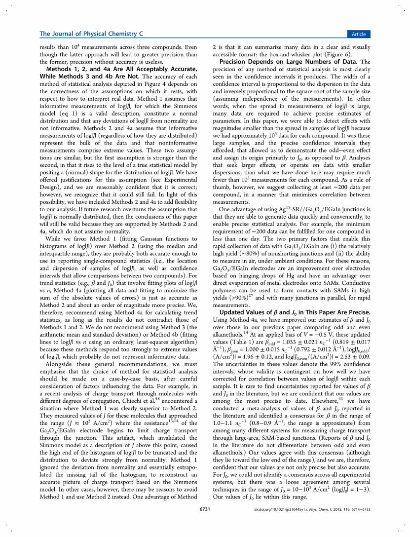
results than 104 measurements across three compounds. Eventhough the latter approach will lead to greater precision thanthe former, precision without accuracy is useless.Methods 1, 2, and 4a Are All Acceptably Accurate,

While Methods 3 and 4b Are Not. The accuracy of eachmethod of statistical analysis depicted in Figure 4 depends onthe correctness of the assumptions on which it rests, withrespect to how to interpret real data. Method 1 assumes thatinformative measurements of log|J|, for which the Simmonsmodel (eq 1) is a valid description, constitute a normaldistribution and that any deviations of log|J| from normality arenot informative. Methods 2 and 4a assume that informativemeasurements of log|J| (regardless of how they are distributed)represent the bulk of the data and that noninformativemeasurements comprise extreme values. These two assump-tions are similar, but the first assumption is stronger than thesecond, in that it rises to the level of a true statistical model bypositing a (normal) shape for the distribution of log|J|. We haveoffered justifications for this assumption (see ExperimentalDesign), and we are reasonably confident that it is correct;however, we recognize that it could still fail. In light of thispossibility, we have included Methods 2 and 4a to add flexibilityto our analysis. If future research overturns the assumption thatlog|J| is normally distributed, then the conclusions of this paperwill still be valid because they are supported by Methods 2 and4a, which do not assume normality.While we favor Method 1 (fitting Gaussian functions to

histograms of log|J|) over Method 2 (using the median andinterquartile range), they are probably both accurate enough touse in reporting single-compound statistics (i.e., the locationand dispersion of samples of log|J|, as well as confidenceintervals that allow comparisons between two compounds). Fortrend statistics (e.g., β and J0) that involve fitting plots of log|J|vs n, Method 4a (plotting all data and fitting to minimize thesum of the absolute values of errors) is just as accurate asMethod 2 and about an order of magnitude more precise. We,therefore, recommend using Method 4a for calculating trendstatistics, as long as the results do not contradict those ofMethods 1 and 2. We do not recommend using Method 3 (thearithmetic mean and standard deviation) or Method 4b (fittinglines to log|J| vs n using an ordinary, least-squares algorithm)because these methods respond too strongly to extreme valuesof log|J|, which probably do not represent informative data.Alongside these general recommendations, we must

emphasize that the choice of method for statistical analysisshould be made on a case-by-case basis, after carefulconsideration of factors influencing the data. For example, ina recent analysis of charge transport through molecules withdifferent degrees of conjugation, Chiechi et al.48 encountered asituation where Method 1 was clearly superior to Method 2.They measured values of J for these molecules that approachedthe range (J ≈ 102 A/cm2) where the resistance13,14 of theGa2O3/EGaIn electrode begins to limit charge transportthrough the junction. This artifact, which invalidated theSimmons model as a description of J above this point, causedthe high end of the histogram of log|J| to be truncated and thedistribution to deviate strongly from normality. Method 1ignored the deviation from normality and essentially extrapo-lated the missing tail of the histogram, to reconstruct anaccurate picture of charge transport based on the Simmonsmodel. In other cases, however, there may be reasons to avoidMethod 1 and use Method 2 instead. One advantage of Method

2 is that it can summarize many data in a clear and visuallyaccessible format: the box-and-whisker plot (Figure 6).

Precision Depends on Large Numbers of Data. Theprecision of any method of statistical analysis is most clearlyseen in the confidence intervals it produces. The width of aconfidence interval is proportional to the dispersion in the dataand inversely proportional to the square root of the sample size(assuming independence of the measurements). In otherwords, when the spread in measurements of log|J| is large,many data are required to achieve precise estimates ofparameters. In this paper, we were able to detect effects withmagnitudes smaller than the spread in samples of log|J| becausewe had approximately 103 data for each compound. It was theselarge samples, and the precise confidence intervals theyafforded, that allowed us to demonstrate the odd−even effectand assign its origin primarily to J0, as opposed to β. Analysesthat seek larger effects, or operate on data with smallerdispersions, than what we have done here may require muchfewer than 103 measurements for each compound. As a rule ofthumb, however, we suggest collecting at least ∼200 data percompound, in a manner that minimizes correlation betweenmeasurements.One advantage of using AgTS-SR//Ga2O3/EGaIn junctions is

that they are able to generate data quickly and conveniently, toenable precise statistical analysis. For example, the minimumrequirement of ∼200 data can be fulfilled for one compound inless than one day. The two primary factors that enable thisrapid collection of data with Ga2O3/EGaIn are (i) the relativelyhigh yield (∼80%) of nonshorting junctions and (ii) the abilityto measure in air, under ambient conditions. For these reasons,Ga2O3/EGaIn electrodes are an improvement over electrodesbased on hanging drops of Hg and have an advantage overdirect evaporation of metal electrodes onto SAMs. Conductivepolymers can be used to form contacts with SAMs in highyields (>90%)27 and with many junctions in parallel, for rapidmeasurements.

Updated Values of β and J0 in This Paper Are Precise.Using Method 4a, we have improved our estimates of β and J0over those in our previous paper comparing odd and evenalkanethiols.14 At an applied bias of V = −0.5 V, these updatedvalues (Table 1) are βodd = 1.033 ± 0.021 nC

−1 (0.819 ± 0.017Å−1), βeven = 1.000 ± 0.015 nC

−1 (0.792 ± 0.012 Å−1), log|J0,odd/(A/cm2)| = 1.96 ± 0.12, and log|J0,even/(A/cm

2)| = 2.53 ± 0.09.The uncertainties in these values denote the 99% confidenceintervals, whose validity is contingent on how well we havecorrected for correlation between values of log|J| within eachsample. It is rare to find uncertainties reported for values of βand J0 in the literature, but we are confident that our values areamong the most precise to date. Elsewhere,41 we haveconducted a meta-analysis of values of β and J0 reported inthe literature and identified a consensus for β in the range of1.0−1.1 nC

−1 (0.8−0.9 Å−1; the range is approximate) fromamong many different systems for measuring charge transportthrough large-area, SAM-based junctions. (Reports of β and J0in the literature do not differentiate between odd and evenalkanethiols.) Our values agree with this consensus (althoughthey lie toward the low end of the range), and we are, therefore,confident that our values are not only precise but also accurate.For J0, we could not identify a consensus across all experimentalsystems, but there was a loose agreement among severaltechniques in the range of J0 = 10−103 A/cm2 (log|J0| = 1−3).Our values of J0 lie within this range.



J0 Explains the Majority of the Odd−Even Effect. Theprecision of Method 4a allows us to conclude, with a level ofconfidence that is high (p = 1.34 × 10−4) but tempered by thepotential effects of correlation between measurements, thatthere is a difference in J0 between odd and even n-alkanethiols.With respect to β, we cannot claim a difference between oddand even n-alkanethiols (p = 0.20). We have shown that thedifference in log|J0| between odd and even n-alkanethiols (log|J0,even| − log|J0,odd| = 0.57) was large enough to explainapproximately 70−80% of the magnitude of the odd−eveneffect. As β is the only other parameter in eq 1 besides J0, adifference in β between odd and even n-alkanethiols is currentlythe strongest candidate to explain the remaining 20−30% of theodd−even effect, but we emphasize caution since we cannotconclude that the difference in β is even significant, let alonelarge. The unexplained portion of the odd−even effect maysimply be the result of uncertainties in β and J0 (determining J0does, after all, require a long extrapolation) or deficiencies inthe Simmons model.The value of J0 represents the contributions to charge

transport of the electrodes and the interfaces between theelectrodes and the SAM. Since the electrodes and (presumably)the AgTS−S interface are identical for both odd and evenalkanethiols, the observation of a significant and large differencein J0 implies that odd and even alkanethiols form different vander Waals interfaces with the Ga2O3/EGaIn electrode.49

Indeed, because of the small tilt angle (the angle of the trans-extended alkyl chain with respect to the surface normal) ofSAMs of n-alkanethiols on Ag (∼12°),1 the terminal −CH3group at the surface of a (trans-extended) SAM should have adifferent orientation, depending on whether the number ofcarbon atoms in the alkyl chain is odd or even. For odd n-alkanethiols, the terminal C−C bond is expected to be roughlyperpendicular to the surface, whereas for even n-alkanethiols,the terminal C−C bond should be approximately parallel to theplane of the surface.49 This subtle difference is apparently largeenough to affect the wave function of charges tunnelingthrough the AgTS-SR//Ga2O3/EGaIn junctionand carefulstatistical analysis is powerful enough to distinguish this effectfrom the myriad of other variables (defects) that affect chargetransport. The fact that such a small change in the surface of theSAM has a noticeable effect on charge transport is a testamentto the (by now, well-known) importance of interfaces inmolecular electronics.Future experiments may settle the question of whether there

is a significant difference in β between odd and even n-alkanethiols and, if so, how large it is. A significant difference inβ would indicate that the tunneling barrier posed by a SAM ofodd n-alkanethiols differs (in shape or height) from that posedby a SAM of even n-alkanethiols. The most we can conclude, atthe moment, is that any difference between odd and even n-alkanethiols with respect to the tunneling barrier (β) has less ofan influence on charge transport than the difference withrespect to the van der Waals interface. We currently have noexplanation for why a terminal C−C bond parallel to thesurface would be more favorable to charge transport than aterminal C−C bond perpendicular to the surface, but weidentify this problem for theoretical study.

■ ASSOCIATED CONTENT*S Supporting InformationAdditional experimental details. This material is available free ofcharge via the Internet at http://pubs.acs.org.

■ AUTHOR INFORMATION

Corresponding Author*E-mail: [email protected].

■ ACKNOWLEDGMENTS

This research was supported by the National ScienceFoundation under Award # CHE-05180055 (measurementsof charge transport and support for W.F.R.) and the U.S.Department of Energy, Office of Basic Energy Sciences,Division of Materials Sciences and Engineering under Award# DE-FG02-OOER45852 (support for M.M.T. and J.R.B.).C.A.N. acknowledges The Netherlands Organization forScientific Research (NWO) for the Rubicon grant supportingthis research and the Singapore National Research Foundationunder NRF Award No. NRF-RF2010-03.

■ REFERENCES(1) Love, J. C.; Estroff, L. A.; Kriebel, J. K.; Nuzzo, R. G.; Whitesides,G. M. Chem. Rev. 2005, 105, 1103−1169.(2) Cui, X. D.; Primak, A.; Zarate, X.; Tomfohr, J.; Sankey, O. F.;Moore, A. L.; Moore, T. A.; Gust, D.; Harris, G.; Lindsay, S. M. Science2001, 294, 571−574.(3) Luo, L.; Frisbie, C. D. J. Am. Chem. Soc. 2010, 132, 8854−8855.(4) Kim, B.; Beebe, J. M.; Jun, Y.; Zhu, X. Y.; Frisbie, C. D. J. Am.Chem. Soc. 2006, 128, 4970−4971.(5) Wang, G.; Kim, T.-W.; Jang, Y. H.; Lee, T. J. Phys. Chem. C 2008,112, 13010−13016.(6) Bumm, L. A.; Arnold, J. J.; Cygan, M. T.; Dunbar, T. D.; Burgin,T. P.; Jones, L. II; Allara, D. L.; Tour, J. M.; Weiss, P. S. Science 1996,271, 1705−1707.(7) Venkataraman, B.; Breen, J. J.; Flynn, G. W. J. Phys. Chem. 1995,99, 6608−6619.(8) Venkataraman, L.; Klare, J. E.; Nuckolls, C.; Hybertsen, M. S.;Steigerwald, M. L. Nature 2006, 442, 904−907.(9) Lee, T.; Wang, W.; Klemic, J. F.; Zhang, J. J.; Su, J.; Reed, M. A. J.Phys. Chem. B 2004, 108, 8742−8750.(10) Kim, T.-W.; Wang, G.; Lee, H.; Lee, T. Nanotechnology 2007,18, 315204−315212.(11) Weiss, E. A.; Kaufman, G. K.; Kriebel, J. K.; Li, Z.; Schalek, R.;Whitesides, G. M. Langmuir 2007, 23, 9686−9694.(12) Chiechi, R. C.; Weiss, E. A.; Dickey, M. D.; Whitesides, G. M.Angew. Chem., Int. Ed. 2008, 47, 142−144.(13) Nijhuis, C. A.; Reus, W. F.; Whitesides, G. M. J. Am. Chem. Soc.2009, 131, 17814−17827.(14) Thuo, M. M.; Reus, W. F.; Nijhuis, C. A.; Barber, J. R.; Kim, C.;Schulz, M. D.; Whitesides, G. M. J. Am. Chem. Soc. 2011, 133, 2962−2975.(15) Nijhuis, C. A.; Reus, W. F.; Barber, J. R.; Dickey, M. D.;Whitesides, G. M. Nano Lett. 2010, 10, 3611−3619.(16) Casella, G.; Berger, R. L. Statistical Inference; Duxbury Press:Belmont, CA, 1990.(17) Bevington, P. R.; Robinson, D. K. Data Reduction and ErrorAnalysis for the Physical Sciences, 3rd ed.; McGraw-Hill: New York,2003.(18) Statistical Methods for Physical Science; Stanford, J. L., Vardeman,S. B., Eds.; Methods of Experimental Physics Series 28; AcademicPress: San Diego, CA, 1994.(19) Simmons, J. G. J. Appl. Phys. 1963, 34, 2581−2590.(20) Huber, P. J. Robust Statistics; Wiley Series in Probability andMathematical Statistics; Wiley and Sons: New York, 1981.(21) Rousseeuw, P. J.; Leroy, A. M. Robust Regression and OutlierDetection; Wiley Series in Probability and Mathematical Statistics;Wiley and Sons: New York, 1987.(22) Weiss, E. A.; Chiechi, R. C.; Kaufman, G. K.; Kriebel, J. K.; Li,Z.; Duati, M.; Rampi, M. A.; Whitesides, G. M. J. Am. Chem. Soc. 2007,129, 4336−4349.



http://pubs.acs.org

mailto:[email protected]

(23) For the purposes of building the model, this assumption isequivalent to assuming that the product, βd, is normally distributed.Assuming that βd is normally distributed may be physically correct, butd is likely to vary to a much greater extent than β since β depends (to azeroeth-order approximation) on the (constant) electronic structure ofthe molecules in the SAM, while d depends on the (variable) densityand type of defects in the components of the junction. We, therefore,proceed under the assumption that β is a constant and d is normallydistributed.(24) The difference between a long tail and an outlier is subjectiveand somewhat arbitrary. The main difference between the two terms isthat long tails are joined to the main peak of the histogram (as a tail isjoined to a body) by a region of continuous data, while outliers areseparated from the main peak of the histogram by “white space” orregions without any data. Also, outliers tend to be fewer in numberthan the data in a long tail. In any case, the distinction has very littlebearing on our analysis. Because both long tails and outliers have asimilar effect on the statistical procedures we use, we can treat themcollectively as “deviations of log|J| from normality”.(25) Chen, J.; Reed, M. A.; Rawlett, A. M.; Jones, L., II; Tour, J. M.Science 1999, 286, 1550−1552.(26) (a) Fisher, G. L.; Walker, A. V.; Hooper, A. E.; Tighe, T. B.;Bahnck, K. B.; Skriba, H. T.; Reinard, M. D.; Haynie, B. C.; Opila, R.L.; Winograd, N.; Allara, D. L. J. Am. Chem. Soc. 2002, 124, 5528−5541. (b) Walker, A. V.; Tighe, T. B.; Cabarcos, O. M.; Reinard, M.D.; Haynie, B. C.; Uppili, S.; Winograd, N.; Allara, D. L. J. Am. Chem.Soc. 2004, 126, 3954−3963.(27) (a) Akkerman, H. B.; de Boer, B. J. Phys.: Condens. Matter 2008,20, 013001. (b) Akkerman, H. B.; Blom, P. W. M.; de Leeuw, D. M.;de Boer, B. Nature 2006, 440, 69−72.(28) Milani, F.; Grave, C.; Ferri, V.; Samori, P.; Rampi, M. A.ChemPhysChem 2007, 8, 515−518.(29) (a) Haag, R.; Rampi, M. A.; Holmlin, R. E.; Whitesides, G. M. J.Am. Chem. Soc. 1999, 121, 7895−7906. (b) Holmlin, R. E.; Haag, R.;Chabinyc, M. L.; Ismagilov, R. F.; Cohen, A. E.; Terfort, A.; Rampi, M.A.; Whitesides, G. M. J. Am. Chem. Soc. 2001, 123, 5075−5085.(30) Slowinski, K.; Fong, H. K. Y.; Majda, M. J. Am. Chem. Soc. 1999,121, 7257−7261.(31) (a) York, R. L.; Nguyen, P. T.; Slowinski, K. J. Am. Chem. Soc.2003, 125, 5948−5953. (b) York, R. L.; Slowinski, K. J. Electroanal.Chem. 2003, 550, 327−336.(32) Rampi, M. A.; Whitesides, G. M. Chem. Phys. 2002, 281, 373−391.(33) Salomon, A.; Boecking, T.; Chan, C. K.; Amy, F.; Girshevitz, O.;Cahen, D.; Kahn, A. Phys. Rev. Lett. 2005, 95, 266807.(34) Salomon, A.; Boecking, T.; Seitz, O.; Markus, T.; Amy, F.; Chan,C.; Zhao, W.; Cahen, D.; Kahn, A. Adv. Mater. 2007, 19, 445−450.(35) Salomon, A.; Bocking, T.; Gooding, J. J.; Cahen, D. Nano Lett.2006, 6, 2873−2876.(36) Dickey, M. D.; Chiechi, R. C.; Larsen, R. J.; Weiss, E. A.; Weitz,D. A.; Whitesides, G. M. Adv. Funct. Mater. 2008, 18, 1097−1104.(37) Cademartiri, L.; Thuo, M. M.; Nijhuis, C. A.; Reus, W. F.;Tricard, S.; Barber, J. R.; Sodhi, R. N.; Brodersen, P.; Kim, C.; Chiechi,R. C.; Whitesides, G. M. manuscript submitted to.(38) Barr, T. L.; Seal, S. J. Vac. Sci. Technol. A 1995, 13, 1239−1246.(39) The concept of resistivity is not well-defined for componentswith nonlinear J(V) characteristics (such as SAMs). For comparing aSAM to the Ga2O3 film, an analog of the resistivity of the SAM at aparticular bias (V) can, however, be estimated, given J through theSAM and the thickness of the SAM (d), using the equation ρ = V/(Jd).(40) Reus, W. F.; Thuo, M. M.; Shapiro, N. S.; Nijhuis, C. A.;Whitesides, G. M. J. Phys. Chem., unpublished experiments.(41) Nijhuis, C. A.; Reus, W. F.; Barber, J. R.; Whitesides, G. M. J.Am. Chem. Soc., submitted.(42) Our statistical model would also be valid under the alternativeassumption that the product βd is normally distributed and J0 isapproximately constant, for then log|J| would still be normallydistributed. Even if J0 is not constant, but log-normally distributed(perhaps due to variations in the width of the tunneling barrier defined

by the van der Waals interface), log|J| would still be the sum of twonormal distributions, which is itself a normal distribution. There are,thus, many scenarios in which log|J| is normally distributed.(43) If a sample has an odd number of elements, then the median isthe value that lies in the middle, when the elements of the sample arearranged in increasing order. If a sample has an even number ofelements, then the median is the average of the two middle values inthe ordered list of elements.(44) Assuming that, for example, the Gaussian mean of log|J| isnormally distributed is not the same as assuming that log|J| itself isnormally distributed; rather, this assumption implies that if manysamples of log|J|, each comprising N measurements, were taken fromthe same population, then the Gaussian means of all samples, takentogether, would collectively conform to a normal distribution.(45) (a) Dale, M. R. T.; Fortin, M.-J. J. Agric. Biol. Environ. Sci. 2009,14, 188−206. (b) Cressie, N. A.; Statistics for Spatial Data; Wiley: NewYork, 1991.(46) Conover, W. J. Practical Nonparametric Statistics; John Wiley andSons: New York, 1980.(47) Galwey, N. W. Genet. Epidemiol. 2009, 33, 559−568.(48) Fracasso, D.; Valkenier, H.; Hummelen, J. C.; Solomon, G. C.;Chiechi, R. C. J. Am. Chem. Soc. 2011, 133, 9556−9563.(49) Tao, F.; Bernasek, S. L. Chem. Rev. 2007, 107, 1408−1453.



statistical tools for analyzing measurements of...

Documents