statistical surface physics: a perspective via computer simulation … · 2015-07-29 ·...
TRANSCRIPT

Rep. Prog. Phys., Vol. 45, 1982. Printed in Great Britain
Statistical surface physics: a perspective via computer simulation of microclusters, interfaces and simple films
Farid F Abraham IBM Research Laboratory, 5600 Cottle Road, San Jose, California 95193, USA
Abstract
We survey selected computer simulations or ‘experiments’ relating to the statistical physics of surface phenomena. An introduction to the Monte Carlo and molecular dynamics simulation techniques is presented, followed by chosen computer simulation applications which have been done mainly at the IBM Research Laboratory over the last several years. The examples are taken from studies of the structure and thermodynamics of microclusters, liquid-vapour and liquid-solid interfaces, and two- dimensional simple films. An attempt is also made to provide an introductory theoreti- cal framework for describing or understanding certain relevant features of a given simulation study. An up-to-date bibliography of the various topics is given at the conclusion.
This review was received in May 1982.
0034-4885/82/101113 +49$08.00 @ 1982 The Institute of Physics 1113
1114 FFAbraham
Contents
1. Preamble 2. The Monte Carlo and molecular dynamics computer simulation methods
of classical statistical mechanics 2.1. The Monte Carlo method 2.2. The molecular dynamics method
3. Simple atomic microclusters 3.1. Physical cluster theory 3.2. Formal definition of physical cluster 3.3. The Monte Carlo procedure for microclusters 3.4. Microcluster properties and their relation to theory and experiment
4.1. Simulation in three dimensions 4.2. Simulation in two dimensions 4.3. Theory for the non-uniform fluid state
5.1. The molecular dynamics simulation 5.2. Perturbation theory for the crystal-melt interface
6.1. The phase diagram of two-dimensional Lennard-Jonesium 6.2. Monte Carlo and molecular dynamics experiments 6.3. Comment on isodensity-isothermal simulations Acknowledgments References Computer simulations in surface science: an incomplete bibliography
4. The planar liquid surface
5 . The crystal-melt interface
6. Two-dimensional simple films
Page 1115
1116 1116 1118 1119 1120 1122 1124 1126 1129 1129 1131 1132 1136 1137 1141 1146 1147 1147 1156 1157 1158 1159

Statistical surface physics 1115
1. Preamble
Computer simulation has added a new dimension to scientific investigation in the rapidly growing fields of surface physics and chemistry. In the last decade, numerous novel innovations in experimental surface science have led to the discovery of a vast richness of structural, thermodynamic and kinetic phenomena for various surface- related systems, such as condensed-phase microclusters in the vapour and on sub- strates, interfaces between coexisting phases, and ‘quasi-two-dimensional’ phases adsorbed on solid surfaces. Challenged by the need to explain these phenomena, the theorist has invented model behaviour which sometimes owes its existence to a broken symmetry or to the lower dimensionality of the physical system and has found, in many cases, that the theoretical analysis can be significantly more complex for this new geometry. As is common in scientific investigation, the validity of a comparison between a particular theoretical prediction and experimental measurement may be sometimes questioned because of the complexity of the experimental interpretation and/or the simplicity of the theoretical model. Furthermore, an investigator may be handicapped in proposing any viable model because of the apparent complexity of the experimental observation, or in testing a theoretical prediction because of a fundamental limitation in the experimental state-of-the-art.
In many ways, computer simulations, or ‘computer experiments’, have alleviated these bottlenecks to progress, one such example being the computer simulation of the properties of physical clusters of a few atoms. Until recently, we have been able to say very little about the microscopic (or molecular) properties of clusters and have resorted to the application of macroscopic thermodynamics or heuristic models of a simplistic nature. However, the heuristic approach requires a successful choice of a model for the problem in hand which represents reasonably well the system of interest and which provides a relatively simple formalism from which numerical quantities can be obtained. While these models provide insights into the origins of certain features of a particular system, they cannot serve to elucidate the molecular structure since this is assumed in one way or another. In a real sense, clusters of a few tens of atoms are ‘all surface’ described by atomic reconstruction grossly different from any macro- scopic crystal or liquid. Hence, attempting to argue that a microcluster may be viewed as a droplet possessing properties of the macroscopic state of matter is highly question- able and has troubled nucleation scientists for decades. In the early 1970s, simulation techniques of classical statistical mechanics using large-scale scientific computers were extended to the study of physical clusters, where only the form of the intermolecular potential energy of interaction between molecules need be assumed and the external conditions, like temperature and pressure, are specified. Detailed information on the structure and thermodynamics of these very small systems finally became available and generated a new level of understanding previously unattainable from laboratory measurements. At present, computer simulation plays a very important role in nucleation research.
In this introductory survey, we will describe two powerful simulation techniques, the Monte Carlo method of Metropolis and the molecular dynamics method. We proceed by describing selected computer simulation applications done at the IBM
1116 FFAbraham
Research Laboratory which should be of general interest to the surface scientist, the examples being taken from studies of microclusters, liquid-vapour and solid-liquid interfaces, and two-dimensional simple films. In the appendix, an up-to-date bibliogra- phy of selected papers on these various topics is provided so that the interested reader may pursue a more complete and unbiased understanding of a particular topic.
2. The Monte Carlo and molecular dynamics computer simulation methods of classical statistical mechanics
2.1. The Monte Carlo method
In classical statistical mechanics, the canonical ensemble average potential energy is given by
where the potential energy of the system U ( f ) depends on the configuration I = ( F l r F 2 , . . . , 7”) of the N particles, and the probability density for the configuration p ( 5 ) is given by
From equations (2.1) and (2.2) we see that ( U ) may be calculated by selecting at random a large number of spatial configurations and averaging the energy over these configurations, weighting each configuration with the appropriate Boltzmann factor. This method is not practicable because the number of configurations required for reasonable averaging is enormous. However, in the Monte Carlo method, the pro- cedure is to select configurations with a frequency proportional to the Boltzmann factor exp (- U ( l ) / k T ) and to average over the selected configurations with equal weight. Metropolis et al (1953) devised a way of doing this, and we will now outline the Metropolis algorithm for a system of spherical atoms in three dimensions.
For a constant density simulation, a system of N particles are placed in an arbitrary initial configuration in a volume V, e.g. a lattice of a chosen crystal packing and of uniform density equal to the experimental density at temperature T ; here, N, V and T a r e fixed. Configurations are generated according to the following rules: (i) select a particle at random; (ii) select random displacements Ax, Ay, Az of the particle’s centre of mass, each uniformly distributed over the interval (-A/2, +A/2); (iii) calculate the change in potential energy SU on displacing the chosen particle by ( A x , Ay, Az); (iv) if SU is negative, accept the new configuration; (v) otherwise, select a random number h uniformly distributed over the interval (0 , l ) ; (vi) if exp (SUIRT) < h, accept the old configuration; (vii) otherwise, the new configuration and the new potential energy become the ‘current’ properties of the system. It is usual to omit the early configurations from the averages, since these would show the effects of the initial ‘non-equilibrium’ configuration and slow the convergence of the averages. The dis- placement parameter A is chosen to optimise convergence; typically A is chosen so that approximately half the attempted moves are actually made, the choice being governed by the density N / V and temperature T of the system, for a given interparticle potential function. If the reader desires, he may go to Barker and Henderson (1976)

Statistical surface physics 1117
for a proof that in a sufficiently long chain generated by these rules configurations c appear with probability proportional to exp ( - U ( c ) / k T ) , as is required for canonical averaging. In figure 1, we present a simple illustration of the Monte Carlo algorithm for an atom at temperature T in an external field.
Given: an atom at a temperature T in an external field U ( x )
I I
XO
Position,x -+
If displaced to the left by A, 6U = U,,, - U&, < 0
accept move x = ~ g - A U = U,,,,.
If displaced to the right by A, 6U = U,,, - Uold > 0,
accept move with probability s e x p (-8UIkT)
if accepted x = x O + A , U=U,,,,
if not accepted x = x g U = Uold.
Continue procedure until good equilibrium averages of (x), ( U ) are obtained.
Note: If T = 0, atomic position will converge to and remain at the potential energy minimum. If T + 03, every position is equally likely, irrespective of U ( x ) .
Figure 1. Illustration of the Monte Carlo algorithm for an atom at temperature T in an external field U ( x ) .
In the constant pressure Monte Carlo method, a configuration of N spherical particles at temperature T and pressure P is represented by 3N coordinates confined within a computational cell of variable volume. A new configuration is generated by selecting a particle at random and giving it a random displacement and by changing the volume of the cell randomly within some predetermined range. The latter step also requires the scaling of all coordinates by the appropriate factor. We denote the total potential energy of the old and new configurations by U and U’ , respectively, and the corresponding volumes of the cell by V and V ’ , respectively. If the quantity
AW = ( U ’ - U ) + P ( V ’ - V ) - N k T In (V’IV) (2 .3 ) is negative, the new configuration is accepted. If it is positive, the new configuration is accepted only with the probability equal to exp ( -AW/kT). Repetition of the procedure gives rise to a chain of configurations distributed in phase space with a probability density proportional to the classical Boltzmann factor.
In order to simulate an infinite bulk with a finite (and small!) number of particles, the technique of employing periodic boundary conditions is used. The basic computa- tional cell of volume V and containing N particles is periodically replicated in the x , y and z dimensions so that the whole of space is filled by periodic images of this basic computational unit. Hence, by considering a limited number of particles,

1118 F F Abraham
configurations of an infinite system are generated (which are, of course, periodic), and ‘surface effects’, which could be large for small N, are circumvented. The cell size does put an upper limit on the range of molecular correlations, but, fortunately, for a large class of problems several tens to a few hundreds of particles are needed to get reliable results. The most direct way to ascertain size effects is to do a chosen simulation experiment with a test size noticeably different from that adopted for the investigation. A similar consideration would apply to the question whether the total number of configurations is adequate in order to establish equilibrium and to obtain good ensemble averages.
In a large part, it is the boundary conditions at the faces of the computational cell that define the problem of interest. For example, by not imposing periodic conditions at two of the opposite faces of the cell and by leaving a ‘vapour space’, we may study the vapour/condensed-phase interface.
In most of our studies we have arbitrarily adopted the Lennard-Jones 12:6 potential function U ( r ) to represent how individual atoms interact in our model universe:
where r is the interatomic separation. This is a respectable interatomic potential for the rare-gas atoms. Our choice of a simple interatomic force law is dictated generally by our desire to investigate the qualitative features of a particular many-body, statistical physics problem common to a large class of real physical systems and not governed by the particular complexities of a unique molecular interaction. If ‘reduced units’ are not used (to be explained later), we will assume that argon systems are being treated.
2.2. The molecular dynamics method
The Monte Carlo method does not generate a true dynamical history of an atomic system, but rather a Markovian chain of spatial configurations according to the rules of the Metropolis algorithm. In contrast to the Monte Carlo method, the molecular dynamics simulation technique yields the motion of a given number of atoms governed by their mutual interatomic interactions, this being calculated by numerical integration of Newton’s equations of motion (Rahman 1964):
d2 N
m - r = - V u ( [ r l - r j l ) f o r i = l , . . . , N . ( 2 . 5 ) dt2 ‘ jPi
In the traditional molecular dynamics experiment, the total energy E for a fixed number of atoms N in a fixed volume V is conserved as the dynamics of the system evolves in time, and the time average of any property is an approximate measure of the microcanonical ensemble average of that property for a thermodynamic state of N, V, E. For certain investigations, it may be advantageous to perform the simulation at constant pressure and/or temperature.
A novel procedure for simulating by molecular dynamics a system under conditions of constant pressure and/or temperature has been proposed by Andersen (1980). But instead of experimenting with this method, we chose to invent a new and different isobaric-isothermal molecular dynamics approach which essentially evolved from our experience with the Monte Carlo method (Abraham I98 lb). Conventional molecular dynamics consists of integrating Newton’s equation of motion to obtain the trajectories

Statistical surface physics 1119
of the atoms, where the total energy is a constant of the motion as the system evolves along its trajectory in phase space. In our isobaric-isothermal molecular dynamics method, we adopt the following two changes from conventional molecular dynamics: (i) in order to simulate a constant temperature, the atomic velocities are renormalised at every time interval T ~ , so that the mean kinetic energy corresponds to the given temperature T ; (ii) in order to simulate a constant pressure, the volume of the computational cell is changed randomly by SV within some prescribed range at every time interval T ~ , requiring the scaling of all the atomic coordinates by an appropriate factor, and with an accompanying total energy change SU. Adopting the Metropolis test, if the quantity
A W = SU + PS V - NkT In (1 + S V/ V) (2.6) is negative, this ‘scaled’ configuration is accepted. If it is positive then this configuration is accepted only with the probability equal to exp (-A W / k T ) . The time evolution of the system is still governed by the numerical integration of the classical equations of motion, but with the velocity renormalisation and position scaling being periodically performed at the specified time intervals. To describe this molecular dynamics method succinctly, the ‘stochastic dynamics’ of the individual atoms in the isobaric-isothermal Monte Carlo method is replaced by the deterministic equations of motion with the added feature of velocity renormalisation-everything else remains the same.
We note that, for equilibrium phases, time averaging of state variables over a sufficient temporal evolution of the system by this molecular dynamics method will yield the proper isobaric-isothermal ensemble averages. Furthermore, it allows for a dynamical (non-equilibrium) relaxation for a system maintained at constant pressure without having to be concerned with specifying an effective piston mass describing the dynamical coupling of the pressure reservoir with the system (such as the Andersen method). In actual fact, this statement is misleading because a value for T~ must be chosen and may be viewed as a dynamical time scale for the volume relaxation. A similar role is played by the mass of the piston. It may be properly stated that this molecular dynamics method does not properly describe the temporal density fluctu- ations of the system at constant pressure but, again, other methods also fail in this respect.
In summary, by specifying the temperature T, volume V (or pressure P ) and intermolecular potential cp, we may simulate the equilibrium and non-equilibrium properties of N particles consistent with the chosen boundary conditions imposed at the faces of the computational cell (e.g. periodic (bulk), free surface, interacting wall, etc) and, therefore, obtain the structure and thermodynamics (e.g. energy, specific heat, pair distribution function, interfacial density profile, etc) of the model system. These thermodynamic and structural data are equivalent to ‘experimental’ results for a well-defined model system and may provide new and unique physical insights unobtainable from present laboratory measurement capability. Furthermore, since there exists no ambiguity in specifying the model system (e.g. the intermolecular potential U is known exactly), the computer experiments provide a unique capability for testing physical theories.
3. Simple atomic microclusters
In this section, we present Monte Carlo simulations of the thermodynamic and structural properties of small rare-gas atom clusters assuming the Lennard-Jones
1120 F F Abraham
potential (Lee et a1 1973, Abraham 1974). First, a formal physical cluster theory for an imperfect gas is outlined that is valid for an arbitrary definition of a ‘physical cluster.’ The role of the definition is stressed since this is an important ingredient for any computer simulation experiment. For a particular definition of the physical cluster, the classical Helmholtz free energy has been found for a range of microcluster sizes up to one hundred atoms and for temperatures ranging from absolute zero to above the bulk melting temperature of Lennard-Jonesium. Selective examples of these extensive Monte Carlo simulations are presented. The results are compared with the capillarity approximation where a ‘liquid’ cluster is modelicd as a uniform density sphere with a surface free energy density equal to the flat-plane surface tension of bulk liquid. We conclude by showing that theoretical nucleation rates based on the Monte Carlo free energies for microclusters are in good agreement with condensation experiments for supersaturated argon.
3.1. Physical cluster theory
In 1938-39, the physical cluster theory of pretransition phenomena was introduced independently by Bijl(1938), Band (1939) and Frenkel(1939). While the basic model is straightforward and would have been understood many years earlier, it appears that the real stimulus for these ideas came from Mayer’s work in 1937 on the activity and virial expansions for the equation of state of an imperfect gas. In these expansions, the coefficients are determined by the well-known cluster integrals. However, the ‘clusters’ in Mayer’s theory cannot be identified with the physical clusters in the Bijl-Band-Frenkel picture.
It is intuitively attractive to suppose that in an imperfect vapour actual physical clusters of atoms exist, that there is an association-dissociation equilibrium between them, and that most of the effects of the intermolecular forces are described by this equilibrium, although there must be residual effects due to interference between different clusters. We emphasise that there is considerable arbitrariness in the definition of a physical cluster. The range of interaction between molecules is infinite so that there is no natural cutoff distance or geometrical size. However, it is possible to carry through a formal theory of physical clusters for any definition of a physical cluster (provided that the definition specifies a unique division of the molecules into different clusters). One might hope that the results of the theory would be independent of the precise definition of physical cluster (within reasonable limits). This would be the case if the vast majority of configurations permitted by a rather non-restrictive definition of cluster actually satisfied a more restrictive condition determined by the intermolecular forces themselves. We shall present evidence that this appears to be the case under certain circumstances.
In any case we now show for any definition of physical cluster that the numbers of clusters of given sizes are determined by the law of mass action (if it is possible to neglect interference effects between clusters 1.
The configuration integral for the total system of Nt molecules in volume Vt may be written as
Q(NJ = (Nt!)-’ . . . exp (-U/RT) drl . . . dr,,
\ -1 c c

Statistical surface physics 1121
where U is the total potential energy and the primed summation notes that, in the second form of equation (3.1), the summation is taken over all sets of numbers of clusters nN, N = 1 , . . , , Nt, that satisfy the constraint
1 NnN = N,. (3.2)
The subscript A identifies a particular cluster containing NA molecules and drA is a short-hand notation for drA,l drA,2 . . . drA,NA ; a particular assignment of NA molecules to the cluster A is assumed. The integration is taken through that region of configur- ation space that actually corresponds to this division into clusters according to whatever definition of a physical cluster we choose to adopt. The total potential energy of the system can be written
u=cuA+ U A p (3.3)
where
(3.4)
and u ~ , ~ ; ~ , ~ is the interaction energy of molecule i of cluster A with molecule j of cluster p. If both the energetic interactions between the clusters (described by UAP) and the geometric or excluded volume interactions can be neglected, then equation (3.1) becomes
where q (N) is the physical cluster configurational integral:
q (N) = (N!)-' I . . . 5 exp ( - u ~ / k T ) drl . . . drN. (3.6) cluster
The most probable set of values {nN} is that which maximises the term in the summation in equation (3.5) subject to the constraint (3.2); it is readily verified that this leads to equation (3.7):
nN/q(N) = {nl/q (111". (3.7)
To go beyond the complete neglect of cluster interactions one can proceed as follows. Suppose that U: is equal to U, when the molecules A l , A 2 , . . . , AN, form a cluster as defined and to +CO otherwise. Also suppose that U;, is equal to U,, when the combined set of molecules (AF) separates exactly into clusters A and p, and to +CO otherwise. Then the partition function can be written in the following form, analogous to the starting point of the Mayer cluster expansion:

1122 F F Abraham
where
f h y = exp (-UL,/kT)- 1. (3.9)
The terms not written in equation (3.8) involve interactions of three or more clusters. This equation provides the basis for a ‘cluster type’ of expansion 01 the partition function for the physical cluster picture of the imperfect vapour; actually, the direct analogy is to the partition function for a gas mixture in which there is also chemical equilibrium between various polymers formed from monomers, with the clusters playing the role of polymers. We note that for certain definitions of a cluster it may be necessary to define quantities like U;,” that are equal to +CO when the combined set (Ayv) does not separate exactly into the clusters A , y , Y while ( A V ) , ( A V ) , (yv) do separate exactly into A , p, etc, and that are zero otherwise. In this case the partition function, equation (3.8), is directly analogous to that for a gas mixture with non-additive interactions.
To the extent that cluster interactions may be neglected, we can in principle compute the cluster partition functions defined by equation (3.6) and then calculate the numbers of clusters nN from equation (3.7).
3.2. Formal definition of physical cluster
In our Monte Carlo calculations we chose to define clusters by the criterion that all atoms of the cluster should lie within a certain distance R, (depending on N ) of the centre of mass of the cluster. Primarily this is for computational convenience. However, we emphasise that it is nevertheless a legitimate definition within the framework of the theory described above; equation (3.8), if written out in full, is an identity. The effect of changing the definition of the cluster is simply to shift some effects of intermolecular forces from the cluster partition function to the cluster interactions (or vice versa). We note that in the case of a gas mixture the atom number centre would be easier to use and possibly more appropriate than the mass centre.
At first sight the imposition of an infinite potential energy barrier when a molecule violates the cluster condition appears to have real physical effects on the nature and structure of the cluster. But this is not a real drawback. Suppose that we possessed a snapshot of a real imperfect gas and that we simply counted clusters; to do this we would have to use a criterion as to whether a given set of molecules form a cluster. Provided that we used the same criterion in both cases, this would lead to the same results as using equations (3.2), (3.6) and (3.7) (providing cluster interactions can be neglected). The act of deciding that N atoms do not form a cluster in the ‘snapshot’ approach plays exactly the same role as imposing the cluster constraint in equations (3.6) or (3.8) or rejecting a configuration in our Monte Carlo calculation. These are simply two different ways of sampling the same ensemble of N-particle configurations. In actual fact we find that, for a given N, at low enough temperatures there is a range of values of R, within which the cluster partition function varies only slightly with R,, so that the apparent arbitrariness of R, is not very important. At higher tem- peratures this is not so, but the theory sketched here indicates that we can still attach meaning to our results.
For computational purposes we adopt the following operational procedure for generating configurations of N- atom clusters. A constraining spherical boundary with radius R, is centred at the centre of mass of the N interacting atoms. The constraint

Statistical surface physics 1123
may be written as
C(RC); Irll S R c for i = 1,. . , , N - 1
where we have used the identity N-1
r L = - C rl. i = l
In this case, equation (3.6) becomes
(3.10)
(3.11)
where this computational cluster of N atoms corresponds to our definition of a physical cluster. The integration in equation (3.1 1) is to be performed over all the configurations of the molecules consistent with the constraint C(Rc).
The Helmholtz free energy of our constrained cluster is given by
Acm(N, Rc) = -kT In zcm(N, Rc)
exp (-uN/kT) dr; . . . drN-1 . (3.12) ' ) 3 ( N - 1 ) ~ 3 / 2
= - k T In('- N!
It is not feasible to evaluate the free energy directly from equation (3.12); however, it is possible to evaluate the derivatives of the free energy with respect to Vc( = &TR :) and T. Given the free energy in a reference state, we can then calculate the free energy by integration. By differentiating equation (3.12) with respect to the constrain- ing volume V, and temperature T, we obtain the 'intrinsic' pressure p and internal energy E of the system. We emphasise the fact that p is the derivative of the free energy with respect to the constraining volume Vc and should not be confused with a thermodynamic pressure of a real system. The results are
where
and also
where

1124 F F Abraham
Here the notation ( )o implies canonical averaging. It is the two functions of equations (3.13(b)) and (3.14(b)) that are obtained from the Monte Carlo calculation.
3.3. The Monte Carlo procedure for microclusters
The Monte Carlo procedure for cluster simulation is summarised in figure 2, where the molecule is pictured as a diatomic molecule. The mean value of any function of the system’s coordinates over all configurations in the chain provides an estimate of the canonical ensemble average of that function. In particular the mean potential energy (UN)o leads to an estimate of the internal energy E, and the mean virial (pVinJo leads, through the virial theorem, to an estimate of the pressure p . The only special feature of our procedure was that an attempted move of a molecule that led to any molecule being at a distance from the centre of mass greater than R, was rejected.
1, Given (old) configumtion
\ 3. Displace and rotate 4 . S h i f t C M t o origin
out of v
5. Calculate energy change
7. Accepted (new) configumtion /----..
Figure 2. The Monte Carlo procedure for the definition of physical cluster presented in $ 3 . 3 .
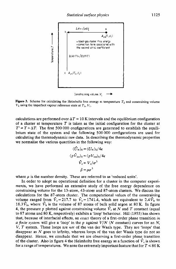
To be close to the ideal-gas reference state, we have chosen T = 160 K and V, = 103Na3 as the starting point in the integration of the p d V , term. At this point we calculate the Helmholtz free energy of an ideal-gas cluster, and add the non-zero second virial coefficient contribution, which is usually less than 0.05%. The procedure for calculating the free energy A,,(N, R,) is shown schematically in figure 3.
The choice of the initial configuration is arbitrary as long as the temperature is sufficiently high. However below 50 K, an arbitrary initial configuration does not rapidly converge to an equilibrium state because of low thermal energy. To avoid this difficulty we have used compact structures of low potential energy. These compact structures are generated from the icosahedron of 55 atoms by the addition or subtrac- tion of atoms and the determination of the relaxed structure. The Monte Carlo
Statistical surface physics 1125
A A = -/pd V,
= Ideal-gas cluster free energy +correction term associated with the second vir ia l coefficient
Constraining volume, V, + Figure 3. Scheme for calculating the Helmholtz free energy at temperature V2 using the imperfect vapour reference state at T1, V1.
and constraining volume
calculations are performed over AT = 10 K intervals and the equilibrium configuration of a cluster at temperature T is taken as the initial configuration for the cluster at T’ = T + AT. The first 500 000 configurations are generated to establish the equili- brium state of the system and the following 500000 configurations are used for calculating the thermodynamic raw data. In describing the thermodynamic properties we normalise the various quantities in the following way:
(” = (Vh7)0/4E
(PQint>o = ( p ~ i n t ) o / 4 ~
Q c = v,/u3 p” = p a 3
where p is the number density. These are referred to as ‘reduced units’. In order to adopt an operational definition for a cluster in the computer experi-
ments, we have performed an extensive study of the free energy dependence on constraining volume for the 13-atom, 43-atom and 87-atom clusters. We discuss the calculations for the 87-atom cluster. The computational values of the constraining volume ranged from pc=217.7 to pc= 1741.4, which are equivalent to 2 .4pb to 18.3pb, where pb is the volume of 87 atoms of bulk solid argon at 80 K. In figure 4, the pressure p plotted against constraining volume FC at N and T constant (equal to 87 atoms and 80 K, respectively) exhibits a ‘loop’ behaviour. Hill (1955) has shown that, because of interfacial effects, an exact theory of a first-order phase transition in a finite system will give a ‘loop’ in the p against V / N (N constant) curves for an N, V, T system. These loops are not of the van der Waals type. They are ‘loops’ that disappear as N goes to infinity, whereas loops of the van der Waals type do not so disappear. Hence, we conclude that we are observing a first-order phase transition of the cluster. Also in figure 4 the Helmholtz free energy as a function of pc is shown for a range of temperatures. We note the extremely important feature that for T s 80 K

1126 F F Abraham
Constraining voIume,Vc
Figure 4. ( a ) Pressure against constraining volume at 80 K and ( b ) Helmholtz free energy against containing volume for several temperature; both figures are for a microcluster of 87 Lennard-Jones ‘argon’ atoms.
the free energy is relatively insensitive for a wide range of constraining volumes cc, i.e. the free energy per atom changes by less than 0.06kT for T = 80 K Qnd 400 S cc 6 1200, and the lower the temperature the‘insensitivity of the free energy to constraining volume increases dramatically. Hence, the cluster free energy is insensitive to a wide range of definitions for a physical cluster, as defined by cc.
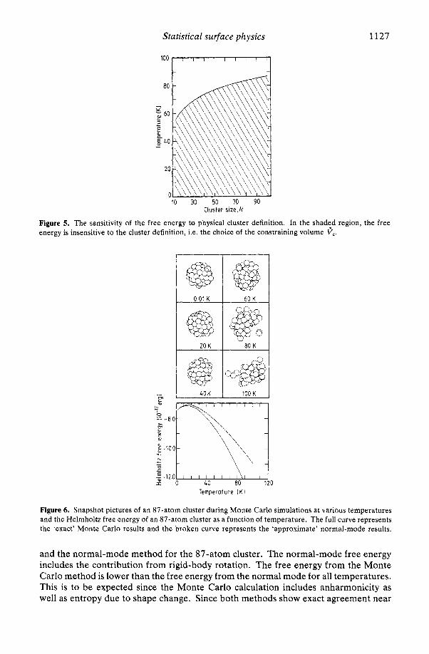
For the ‘standard’ constraining volume in the Monte Carlo study, we have chosen cc = 5 Fb, the volume at which the pressure becomes approximately zero in the ‘loop’ for the 87-atom cluster at 80 K. This choice of the constraining volume gives our computational definition of a physical cluster. Because of the fact that at sufficiently low temperatures the free energy of the clusters is almost independent of the radius of the defining sphere over a fairly wide range suggests strongly that at low temperatures only compact, roughly spherical clusters are important. In figure 5 the shaded area shows the region in which this is so. In the upper region of figure 5 the free energy depends strongly on the sphere radius, so that estimates of cluster concentrations depend critically on the definition chosen. However, within the framework of the theory developed, the results may be regarded as meaningful even in this region.
3.4. Microcluster properties and their relation to theory and experiment
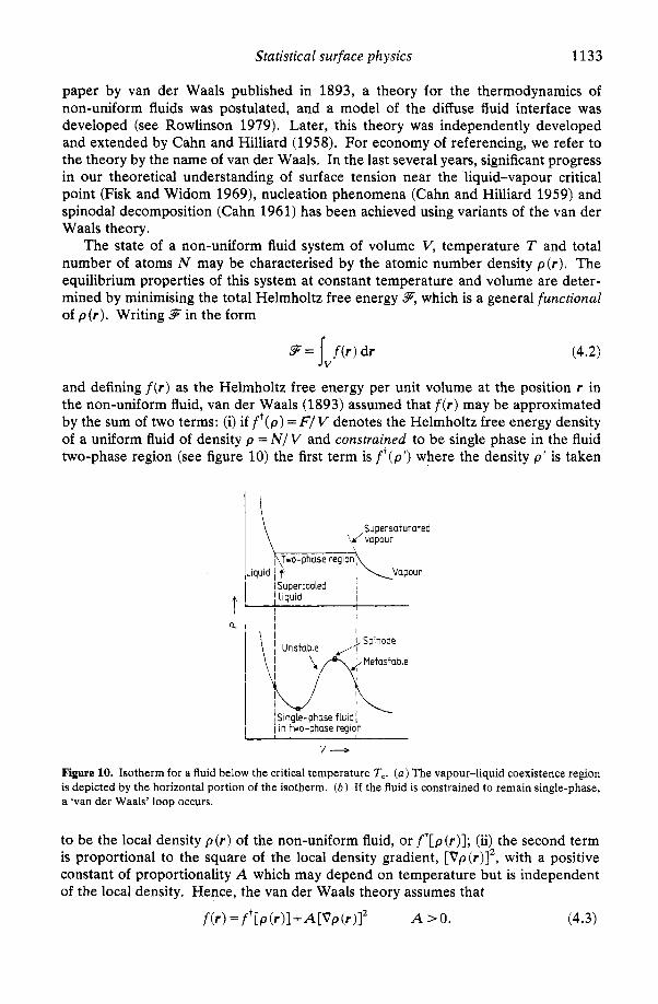
We choose only one cluster size of Lennard-Jones atoms to illustrate the results of the Monte Carlo experiments. In figure 6 we present snapshot pictures of the 87-atom cluster that were taken during the Monte Carlo simulations at various temperatures. We note the expected thermal expansion as well as the shape distortion with increase in temperature. Below 30-40 K, the clusters are essentially crystalline and the site exchange of any two molecules is not observed. A liquid-like state is gradually achieved, the transition occurring at higher temperatures for larger cluster sizes. Also in figure 6 we present the Helmholtz free energy with respect to the centre-of-mass reference frame as a function of temperature obtained using the Monte Carlo method
Statistical surface physics 1127
10 30 50 70 90
Figure 5. The sensitivity of the free energy to physical cluster definition. In the shadtd region, the free energy is insensitive to the cluster definition, i.e. the choice of the constraining volume V,.
[Luster size, N
0 01 K
40 K
60 K 1
“ 8 0 K I
100K
Temperature I K t
Figure 6. Snapshot pictures of an 87-atom cluster during Monte Carlo simulations at various temperatures and the Helmholtz free energy of an 87-atom cluster as a function of temperature. The full curve represents the ‘exact’ Monte Carlo results and the broken curve represents the ‘approximate’ normal-mode results.
and the normal-mode method for the 87-atom cluster. The normal-mode free energy includes the contribution from rigid-body rotation. The free energy from the Monte Carlo method is lower than the free energy from the normal mode for all temperatures. This is to be expected since the Monte Carlo calculation includes anharmonicity as well as entropy due to shape change. Since both methods show exact agreement near

1128 F F Abraham
0 K for all cluster sizes, a reference state based on the normal-mode results at 1 K may replace the ideal-gas cluster state in calculating the free energy of a cluster. In general, the difference in the free energy for both methods is about 5-10% at 50 K. This is in contrast to the fact that the potential energy of the clusters increases by about 20-40% from 0 to 50 K. Also, the difference in the free energy at 100 K is 20-25% while the potential energy increases by 55-75'/0 from 0 to 100 K. Thus, we conclude that the normal mode method fortuitously gives a better estimate for the free energy than would be expected from the potential energy comparisons because it does not account for the entropy due to thermal expansion as well as shape change.
There are two rival physical cluster theories-the Becker-Doring (1935) theory and the Lothe-Pound (1962) theory-both of which modelled the small 'liquid' cluster as a uniform density sphere with a surface tension equal to the flat-plane surface tension of the bulk liquid, i.e. both theories invoke the capillarity approximation. We will not reproduce the details of these two theories but refer the reader to Abraham (1974). In tables 1 and 2, we compare the total Helmholtz free energies predicted by these approximate theories with the exact results of the Monte Carlo study of physical clusters. In both tables, the agreement of the approximate Becker-Doring free energies FB-D with the exact Monte Carlo free energies Fexact is not good. On the other hand, the agreement between the approximate Lothe-Pound free energies and Fexact is impressive at both temperatures. Prior to the Monte Carlo experiments, it was very difficult to ascertain the relative merits of these two approximate theories. However, it would not be incorrect to attribute the good agreement of the Lothe- Pound theory with the exact results as fortuitous.
Table 1. Comparison of capillarity values with Monte Carlo results at 70 K for argon clusters.
Becker-Doring lot he-Pound
N Fexact(N) FB-D@" - Fe,,&') FL-PO" -Fe,,,, (NI
13 -148.9kT 37.7kT 1.9kT 43 -514.8kT 43.lkT 3.0kT 60 -731.7kT 45.4kT 3.9kT 70 -859.6kT 45.2kT 3.lkT 80 -987.9kT 44.4kT 1.8kT 87 -1079.6kT 45.lkT 2.lkT
Table 2. Comparison of capillarity values with Monte Carlo results at 80 K for argon clusters.
~
13 -146.0kT 34.5kT O.OkT 43 -497.6kT 41.8kT 2.7kT 60 -703.9kT 44.7kT 4.2kT 70 -825.0kT 44.7kT 3.6kT 80 -947.0kT 44.6kT 3.0kT 87 -1034.8kT 46.5kT 4.7kT

Statistical surface physics 1129
Recently, Garcia and Torroja (198 1) have compared the theoretical homogeneous nucleation rates using the Monte Carlo cluster free energies with experimental measurements for argon over a wide range of pressures and temperatures. In figure 7, we present their comparison and note good, but not perfect, agreement between theory and experiment.
Figure 7. Comparison of different calculations with experimental data for the onset of condensation. Broken curves: classical theory; full curves: Monte Carlo work. In each case, the lower and upper curves are for a nucleation rate of 1 and lo6 cm-3 s-’, respectively. Open triangles and full circle are for pure argon, and open circles are for argon in a helium carrier gas (from Garcia and Torroja 1981).
An obvious next study is to calculate the thermodynamic and structural properties of ‘real’ argon clusters, i.e. use an accurate argon potential that includes three-body contributions instead of the qualitative Lennard-Jones potential. This would provide a critical comparison between laboratory measurement, computer simulation and theory.
4. The planar liquid surface
The determination of the liquid-vapour interfacial structure is only beginning to be realised by present-day experimental innovations in the laboratory (Beaglehole 1979). In contrast, the theoretical description of this interface encompasses almost a century of scientific activity, dating back to van der Waals’ classic treatise published in 1893. Because of the experimental bottleneck, validation of various theories remained impossible until a decade ago. It was because of computer simulations of the planar liquid surface beginning in the mid-1970s that progress in our understanding of this important physical system could be realised. We will describe certain successes in this area of research.
4.1. Simulation in three dimensions
One of the first computer simulations of the liquid surface caused quite a stir in this field (Lee et al 1974); it suggested the possible existence of ‘surface layering’ of several

1130 F F Abraham
atomic diameters (-7 layers) into liquid argon from the free surface. However, we showed that this was an artefact of the extremely slow convergence of the liquid-vapour interfacial density profile (Abraham et a1 1975). We will present this correct Monte Carlo simulation.
We adopted a system of slab shape composed of 256 Lennard-Jones atoms which has two free surfaces perpendicular to the z axis. The z = 0 plane of the slab corresponded to the ‘z’ centre of mass of the 256 atoms, and an attempted move of an atom that led to any atom being at a distance from the z centre of mass greater than 12 1 = zm was rejected. The standard periodic boundary conditions were imposed with respect to translations parallel to the free surface. The initial atomic configuration of the slab was constructed in the following way. A Monte Carlo bulk liquid simulation was performed for a cube of 64 atoms at 84 K, the edge of the periodic cube being 1, = 14.82 A ( 4 . 4 ~ ) . Approximately 1.2 x lo6 configurations were generated, or 18 750 configurations per atom. This number of configurations was required to get a constant average energy for the bulk. By replicating the last bulk configuration four times in the z direction with a spatial period equal to the linear dimension of the periodic cube, we constructed the initial slab configuration for the free surface calculation (see figure 8). Because of the periodic conditions used in the bulk simulation, matching between faces of two neighbouring cubes is consistent with the equilibrium bulk configuration. Further simulation was then required with the constructed slab in order to allow the two free surfaces to relax to equilibrium. The thickness of the unrelaxed slab was I, = 41, = 59.3 A ( 1 7 . 5 ~ ) . The constraint distance zm equalled 90 A, or a vapour region of -15 A per surface was allowed.
2 : -2, 2-2,
I b i Surface density prof i le Buik density prof i le PIXI ply1
0 12 24 36 0 6 12 0 6 12 Distance,z ( A i xiA, YIA,
Figure 8. ( a ) Schematic drawing of the construction of the liquid slab from the equilibrium bulk liquid cube for the Monte Carlo computation of the liquid-vapour free surface. The symbol - implies periodic boundary conditions. ( 6 ) The surface density p ( z ) and bulk density profiles p ( x ) and p ( y ) for a Lennard- Jones fluid at 84 K obtained from Monte Carlo averaging over 0.8, 2.6, 4.2 and 6.2 million configurations of a 256-atom system.

Statistical surface physics 1131
Before statistics from the numerical experiment were collected, an additional 1.7 x lo6 configurations were simulated in order to allow the relaxation of the two free surfaces. In figure 8 we also present the density profiles for a free surface p ( z ) obtained by averaging the densities of the slab which are an equal absolute ‘z’ distance from the origin (or centre of mass), i.e. p ( z ) = 0.5b (lz 1) + p (-12 I)]. We also include the density profiles p (x) and p (y ) which are representative of the bulk liquid density profile of the slab. Four sets of density profiles ( p ( z ) , p ( x ) , p ( y ) } are presented and represent statistical averaging of atomic locations for 0.8, 2.6, 4.2 and 6.2 million configurations, respectively. While the average potential energy per atom was essen- tially constant over the configurational averaging, -(0.807 f 0.001) x erg, the convergence of the density profiles is obviously very slow, both for the surface profile, p ( z ) , and for the bulk profiles, p (x) and p (y ).
While some ‘structure’ remains in all of the density profiles (p ( z ) , p (x), p (y )} after 6.2 million configurations, we make the following observations: (i) the number of ‘layers’ or ‘humps’ in p ( z ) are three, diminishing from an original eight humps; (ii) the amplitudes of the humps in p ( z ) are comparable to those in p ( x ) ; (iii) their presence, while existing through all of the configurational averages, has diminshed monotonically and markedly; (iv) the amplitudes and number of humps are approxi- mately a factor of three smaller than what was reported by Lee et a1 (1974). The persistence of apparent layer-like structures over long Monte Carlo chains (even in bulk fluid!) is remarkable, but we must conclude that such structures do not exist in a true canonical average.
We note that in a computer experiment the periodic planar boundary conditions in (x, y ) prevent the occurrence of surface (or capillary) waves of wavelength greater than the width of the computational cell I, or other than integral divisions of I,. As a consequence the computer experiment is more nearly simulating the ‘bare’ or ‘intrinsic’ surface profile, i.e. a liquid surface where essentially most of the capillary fluctuations are suppressed. Chapela et a1 (1977) have performed simulations which vary the surface area and have found a slow increase in the interfacial thickness with increase in surface dimension. This finding gives support to the Buff et a1 (1965) capillary theory for the liquid-vapour interface, but it is presently too difficult to establish quantitative agreement.
4.2. Simulation in two dimensions
There is a question whether one of the consequences of dimensionality on phase equilibria is that fluid-phase coexistence between a liquid and a vapour may not exist for an atomic system that is strictly two-dimensional (Frenkel and McTague 1979). Recently, we have demonstrated the reality of such fluid-phase coexistence by simu- lating the liquid-vapour interface of a two-dimensional Lennard-Jones fluid at a temperature of 53.14 K (Abraham 1980a).
The computer simulation procedure is identical to that adopted for our three- dimensional liquid-vapour interface, with the obvious constraint that the system remains two-dimensional. In figure 9 we present ‘snapshot pictures’ of the (x ,z) atomic positions of the 256 Lennard-Jones atoms for the denoted sequence of configur- ations in our Monte Carlo simulation. We make special note of the prominent demarkation between the regions of liquid and vapour and also of the diversity of line topologies defining the two-dimensional liquid-vapour interface. It is the canoni- cal averaging of these interfacial configurations that results in an interfacial width in

1132 F F Abraham
5 0x106
7.5 x10⁶
Figure 9. Snapshot pictures of the ( x , z ) atomic positions of the 256 Lennard-Jones atoms for the denoted sequence of configurations in the Monte Carlo simulation for the two-dimensional liquid-vapour interface. The horizontal broken lines of the computational box depict periodic boundary conditions and the vertical full lines depict hard walls.
p (z) of - 13-15 A. Certainly, the stability of the liquid ribbon to fragmentation from such dramatic surface undulations attests to the reality of the two-phase coexistence.
If we extend the Buff-Lovett-Stillinger capillary theory for the liquid-vapour interface to two dimensions, we find that the interfacial width d is given by
where L is the length of the line interface, a. is some characteristic length of the order of an interatomic distance in the liquid state and y is the interfacial line tension. Making the drastic assumption that the -15 A interfacial width that we measured in the Monte Carlo experiment strictly arises from infinitesimal capillary fluctuations with wavelengths less than 1,(=31.7 A), we may use equation (4.1) to estimate the width of a two-dimensional liquid-vapour interface with a macroscopic line dimension, e.g. for an interfacial length L = 1 cm, the interfacial thickness d zz 3 p m , in vivid contrast to the size of the liquid-vapour interface for three-dimensional coexistence.
Of course, without the imposed geometrical constraints of our model system, the ribbon geometry would be unstable to disc (two-dimensional droplet) formation since there is no physically operative analogue to the gravitational field which allows the existence of a stable planar liquid-vapour interface. However, this fact does not change the conclusions of this study; in particular, liquid-vapour coexistence in two dimensions does exist.
4.3. Theory for the non-uniform fluid state
For the stable equilibrium state in the two-phase region, the coexistence of liquid and vapour requires the presence of an 'interface' which is characterised by a density non-uniformity joining the constant density liquid and vapour phases. In a classic
Statistical surface physics 1133
paper by van der Waals published in 1893, a theory for the thermodynamics of non-uniform fluids was postulated, and a model of the diffuse fluid interface was developed (see Rowlinson 1979). Later, this theory was independently developed and extended by Cahn and Hilliard (1958). For economy of referencing, we refer to the theory by the name of van der Waals. In the last several years, significant progress in our theoretical understanding of surface tension near the liquid-vapour critical point (Fisk and Widom 1969), nucleation phenomena (Cahn and Hilliard 1959) and spinodal decomposition (Cahn 1961) has been achieved using variants of the van der Waals theory.
The state of a non-uniform fluid system of volume V, temperature T and total number of atoms N may be characterised by the atomic number density p ( r ) . The equilibrium properties of this system at constant temperature and volume are deter- mined by minimising the total Helmholtz free energy 9) which is a general functional of p ( r ) . Writing 9 in the form
9= f ( r ) dr I, (4.2)
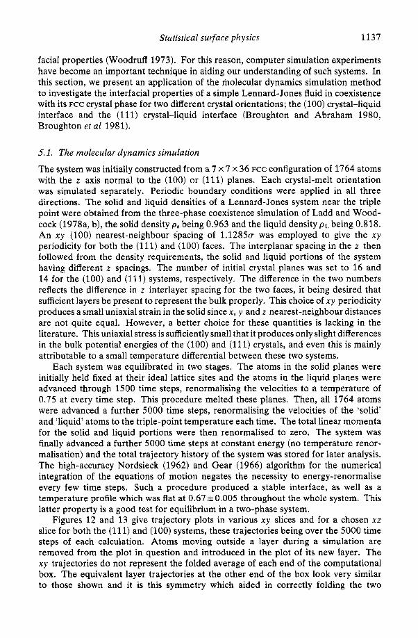
and defining f ( r ) as the Helmholtz free energy per unit volume at the position r in the non-uniform fluid, van der Waals (1893) assumed that f ( r ) may be approximated by the sum of two terms: (i) if f ' ( p ) = F/ V denotes the Helmholtz free energy density of a uniform fluid of density p = N/ V and constrained to be single phase in the fluid two-phase region (see figure 10) the first term is fT(p ' ) where the density p ' is taken
Supersaturated L( vapour
Liquid 1 Vapour I Supercooled , !Liquid I
cl.
v+
Figure 10. Isotherm for a fluid below the critical temperature T,. ( a ) The vapour-liquid coexistence region is depicted by the horizontal portion of the isotherm. ( b ) If the fluid is constrained to remain single-phase, a 'van der Waals' loop occurs.
to be the local density p ( r ) of the non-uniform fluid, or f ' [ p ( r ) ] ; (ii) the second term is proportional to the square of the local density gradient, [Vp(r)]' , with a positive constant of proportionality A which may depend on temperature but is independent of the local density. Hence, the van der Waals theory assumes that
f ( r ) =f+b ( r ) l + A [ V p (41' A >O. (4.3)

1134 F F Abraham
Equation (4.3) may be argued by assuming that f ( r ) is, in general, a functional of the non-uniform fluid density, performing a functional Taylor expansion about the local density p(r) , and truncating the series at second order. There is no real justification for having truncated what might have been expected to be, more generally, an infinite series of powers and products of the first and higher derivatives of the density function. This is one reason for believing that the van der Waals theory is only valid when there exists very small density variations from uniformity over very large spatial regions (e.g. the liquid-vapour interface near the critical point). For problems like the thermodynamic description of the liquid-vapour interface near the triple point, the van der Waals theory would not be applicable.
In the spirit of van der Waals’ approach, we have proposed the following theory for the free energy of a non-uniform fluid system (see Abraham 1979). We take, as a starting point, van der Waals’ assumption that the free energy densityf(rl) at position rl may be written as the sum of two terms, and the first term is the single-phase free energy density of a uniform fluid evaluated at the local density p (rl), i.e.
f(rd =f+[P(rl)l+Sf(rl , {PI). (4.4)
We note that Sf(rl,{p}) should be some functional of the density field, denoted symbolically by { p } , which ‘corrects’ the local free energy density assumption expressed by the first term. For simple fluids, the free energy density f t ( p ) may be calculated using successful perturbation theories of the uniform liquid state (Barker and Hender- son 1976). The perturbation theories consider the interatomic potential of the form
U = U r + U P (4.5) where K~ is the interatomic potential of the unperturbed (or reference) fluid and u p is the perturbation potential. An explicit expression for equations (4.2) and (4.4) may be easily obtained by the functional Taylor expansion technique. We write that the total Helmholtz free energy 9 is a general function of p and U, i.e.
9= 9 { p , U}. (4.6) Assuming equation (4.5) and expanding 9 about ur , we obtain
Recognising that the pair correlation functional g2 is defined by
equation (4.7) becomes
Making the ‘local’ assumptions that
(4.10)
(4.11)
and

Statistical surface physics 1135
we obtain the ‘generalised van der Waals’ expression:
We may obtain the van der Waals expression by expanding p (r + r ’ ) in a Taylor
p ( r + r ’) = p (r ) -t r ’ * Vp (r ) + +(rf v)’p (r ) + , . . (4.13)
and truncating the expansion for terms of higher than second order in the gradients. Because U and g z are rotationally invariant, equation (4.12) becomes
f ( r ) = f+[p (r)I + P ( r ) B V’P ( r )
series about the point r :
(4.14)
where
J V (4.15)
Integrating equation (4.14) over volume V we obtain the total free energy 9, equation (4.2). By applying the divergence theorem to the volume integral of the term p (r)BV’p ( r ) , we obtain for 9
Jv
where
(4.16)
(4.17)
This is simply the van der Waals theory where, now, we have an explicit expression for A, and it is similar to the one obtained by Cahn and Hilliard (1958) for regular binary solutions if B is not dependent on density, i.e. A = -B. From this development, we are able to appreciate the fact that the van der Waals theory is only valid when there exists very small density variations from uniformity over a very large spatial region. Actually, the higher-order terms in the expansion diverge for the Lennard- Jones power law! Recently, Singh and Abraham (1977) have gone beyond adopting the ‘local’ approximations by developing a perturbation theory for non-uniform fluids which accounts for the ‘non-local’ contributions neglected by assuming equations (4.10) and (4.11). But equation (4.12) is qualitatively accurate as well as being conceptually and computationally much simpler. In figure 11, comparison of the liquid-vapour density profile between computer experiment and various theories is presented near the triple point. While the Singh-Abraham theory gives the best agreement, the generalised van der Waals prediction of Abraham is quite acceptable. As the critical point is approached, the predictions of the various theories will be indistinguishable.
We have mentioned earlier that the computer simulations do not include important contributions from capillary fluctuations. In the capillary theory, the actual interfacial width is a direct consequence of statistically averaging the normal distortions of an ‘intrinsic’ or ‘bare’ interface, these distortions being uniquely identified as capillary waves. This model results in the width depending explicitly on the dimension of the surface area and the strength of the external gravitational field. If the effect of

1136 F F Abraham
0 I , , , , ,
-12 -8 - 4 0 4 8 12 D is tance ,z l~J
Figure 11. Comparison of liquid-vapour profiles predicted by various theories with Monte Carlo simulation shown in figure 8 (6). - - -, Monte Carlo; - . -, generalised van der Waals theory; -, Singh-Abraham; --_ , van der Waals theory.
the gravitational field is ignored, the interfacial width diverges at any temperature as the surface area tends to infinity, e.g. see equation (4.1) for a two-dimensional interface. This behaviour is in sharp contrast to the interfacial width results using the van der Waals ‘like’ theories previously discussed where, for temperatures below the critical temperature, the width is finite and independent of the size of the surface area. There is no basic contradiction between these two results; it is simply that the ‘intrinsic’ width of the capillary model, usually taken as a sharp discontinuity in density between the bulk phase densities, can be identified as the interfacial width given by the predictions of a van der Waals theory. One may legitimately question the validity of this last statement and consequently the agreement between the generalised van der Waals theory (in particular the Singh-Abraham theory) and the Monte Carlo experiments. The answer is that, for both theory and computer experiment, the capillary wave fluctuations have not been properly accounted for. In the theory, no explicit consideration was given to interfacial configurations that deviate from planar- ity, i.e. the interfacial correlation functional is approximated by the bulk phase correlation function. In the computer simulation, the periodic planar boundary condi- tions in ( x , y ) prevent the occurrences of inhomogeneities which are longer than the side Lo of the computational cross section or are other than integral divisions of Lo; in our case Lo= 15 A and essentially all capillary wave fluctuations are suppressed. Hence, the generalised van der Waals theory and the computer simulation properly described the intrinsic or bare profile defined in the capillary model.
An interesting computer experiment would be to investigate the dependence of interfacial width d on surface size L for a two-dimensional liquid-vapour system, the reason being that theory predicts a square-root dependence of d on L (equation (4.1)) instead of the logarithmic dependence for the three-dimensional liquid-vapour system.
5, The crystal-melt interface
The solid-liquid interface, being bounded by two dense phases, is difficult to study in the laboratory. The experiments often rely upon indirect measurement of the inter-
Statistical surface physics 1137
facial properties (Woodruff 1973). For this reason, computer simulation experiments have become an important technique in aiding our understanding of such systems. In this section, we present an application of the molecular dynamics simulation method to investigate the interfacial properties of a simple Lennard-Jones fluid in coexistence with its FCC crystal phase for two different crystal orientations; the (100) crystal-liquid interface and the (111) crystal-liquid interface (Broughton and Abraham 1980, Broughton et a1 1981).
5.1. The molecular dynamics simulation
The system was initially constructed from a 7 x 7 x 36 FCC configuration of 1764 atoms with the z axis normal to the (100) or (111) planes. Each crystal-melt orientation was simulated separately. Periodic boundary conditions were applied in all three directions. The solid and liquid densities of a Lennard-Jones system near the triple point were obtained from the three-phase coexistence simulation of Ladd and Wood- cock (1978a, b), the solid density p s being 0.963 and the liquid density pL being 0.818. An x y (100) nearest-neighbour spacing of 1 . 1 2 8 5 ~ was employed to give the x y periodicity for both the (111) and (100) faces. The interplanar spacing in the z then followed from the density requirements, the solid and liquid portions of the system having different z spacings. The number of initial crystal planes was set to 16 and 14 for the (100) and (111) systems, respectively. The difference in the two numbers reflects the difference in z interlayer spacing for the two faces, it being desired that sufficient layers be present to represent the bulk properly. This choice of x y periodicity produces a small uniaxial strain in the solid since x, y and t nearest-neighbour distances are not quite equal. However, a better choice for these quantities is lacking in the literature. This uniaxial stress is sufficiently small that it produces only slight differences in the bulk potential energies of the (100) and (111) crystals, and even this is mainly attributable to a small temperature differential between these two systems.
Each system was equilibrated in two stages. The atoms in the solid planes were initially held fixed at their ideal lattice sites and the atoms in the liquid planes were advanced through 1500 time steps, renormalising the velocities to a temperature of 0.75 at every time step. This procedure melted these planes. Then, all 1764 atoms were advanced a further 5000 time steps, renormalising the velocities of the ‘solid’ and ‘liquid’ atoms to the triple-point temperature each time. The total linear momenta for the solid and liquid portions were then renormalised to zero. The system was finally advanced a further 5000 time steps at constant energy (no temperature renor- malisation) and the total trajectory history of the system was stored for later analysis. The high-accuracy Nordsieck (1962) and Gear (1966) algorithm for the numerical integration of the equations of motion negates the necessity to energy-renormalise every few time steps. Such a procedure produced a stable interface, as well as a temperature profile which was flat at 0.67 f 0.005 throughout the whole system. This latter property is a good test for equilibrium in a two-phase system.
Figures 12 and 13 give trajectory plots in various x y slices and for a chosen xz slice for both the (111) and (100) systems, these trajectories being over the 5000 time steps of each calculation. Atoms moving outside a layer during a simulation are removed from the plot in question and introduced in the plot of its new layer. The x y trajectories do not represent the folded average of each end of the computational box. The equivalent layer trajectories at the other end of the box look very similar to those shown and it is this symmetry which aided in correctly folding the two

1138 FFAbraham
xy cross section
Layer 5 Layer 6 Layer I Layer 8
xz cross section
2 3 4 5 6 1 (1111 7 6 5 4 3 2 1
Figure 12. Trajectories of atoms during the (1 11) crystal-melt simulation for various x y slices parallel to the interface and for a xz slice perpendicular to the interface. The x y slices are numbered under the x z trajectory picture. Any atom entering a slice, at any time during the simulation, is represented so long as it remains in the slice.
Figure 13. Trajectories of atoms during the (100) crystal-melt simulation for various x y slices parallel to the interface and for a x z slice perpendicular to the interface. The xy slices are numbered under the xz trajectory picture. Any atom entering a slice, at any time during the simulation, is represented so long as it remains in the slice.
interfacial systems to obtain z-dependent density profiles. Layer 6 of the (111) and layer 7 of the (100) appear to behave very similarly. A small amount of diffusion occurs (the exact amount of which is shown in figure 14) but particles nevertheless spend most of their time vibrating about their lattice sites. It is difficult to speculate whether those layers represent two-phase coexistence in two dimensions; certainly some regions are more mobile than others. The next layer up, in each case, definitely

Statistical surface physics 1139
I
. e . . ? ~ 0 0 0 0 8 , I I
represents a two-dimensional liquid, but both for the (111) and the (100) systems (especially for the (11 1)) careful examination of the x y trajectories indicates higher residence times in the position of the ideal lattice sites. This is not surprising; the field of the layer beneath, itself virtually crystalline, will produce potential energy minima in their positions. These trajectories plots, therefore, indicate that the transi- tion from crystal to liquid is rather sharp. In this respect, the trajectory plots are a sensitive measure of the position of the interface.
Figure 14 gives x y diffusion coefficients for the (111) and (100) systems. These coefficients are effective two-dimensional (2D) diffusion coefficients and are obtained from x y mean square displacement against time data for a given layer. When particles move from one layer to another they are excluded from the calculation of the diffusion coefficient. The two systems have been shifted with respect to one another to give maximum overlap in the interface region. The origin occurs at layer 6 for t!x (111) system and layer 7 for the (100) system. It is these layers which one might guess represent the last crystalline layers before the onset of the disorder of the liquid. In fact, the x y trajectory analysis and two-dimensional radial distribution function data supports this assignment. Thus, the interface again appears to be approximately four layers wide. The liquid bulk diffusion coefficient has a value of -0.033 in reduced units and this compares favourably with experimental values for liquid argon at the triple point. An important observation arising from figure 14 is that the width of the interface is very similar for both the (111) and (100) systems.
I
l o
I . , 0 1 1 I
Distance, z/a
Figure 14. Diffusion coefficients against z coordinate (reduced units): 0 (111) interface, 0 (100) interface. The two systems have been shifted so that the z origin is situated in both cases at the equilibrium position of the last crystalline layer (layer 6 for the (111) system and layer 7 for the (100) system). The non-zero diffusion coefficient in the crystal is due to a (slow) global translation of the crystal. The broken line represents the bulk diffusion coefficient of liquid argon near the triple point.
In figure 15, we present the atomic number density profile p ( z ) , the potential energy density profile cp (2) and the temperature profile T ( z ) for the (100) crystal-liquid interface and the (1 11) crystal-liquid interface, respectively. Also included in these figures are the ‘coarse-grain-averaged’ profiles of p ( z ) , cp ( z ) and T ( z ) averaged between minima in the number density profile. The profiles represent an averaging of the statistics for the two interfaces of a given simulation about the symmetry plane and, in effect, is equivalent to a total time averaging of 10 000 time steps for obtaining the equilibrium properties of a single interface. The temperature profiles

1140 F F Abraham
la1
4
2
0
20
10
0 P"''''!J liii)
0 4 8 12 16 .?/U
4
2
0
20
10
0 0.8
0 4 0 4 8 12 16
ZlU
Figure 15. The atomic number density profile p ( z ) (i), the potential energy density profile 9(2) (ii) and the temperature profile T ( z ) (iii) for the Lennard-Jones (111) ( a ) and (100) ( b ) crystal-melt interface. Superimposed on each profile is the coarse-grain averaged profiles over a Az increment comparable to one lattice spacing. The quantities are expressed in reduced units.
are remarkably constant throughout the interfaces and correspond to an average temperature of 0.670 f 0.005. Also, the potential energy density profiles closely mimic the number density profiles for the respective interfaces. The separation between the crystalline solid phase and the liquid phase is denoted by the vertical dashed line on the atomic density profile. This separation is suggested by the zero minima unique to the crystal plane profiles because of negligible interplanar exchange and insignificant thermal broadening overlap, as well as the non-zero minima in the liquid phase arising from significant interplane atomic mobility. This statement is supported by detailed trajectory analysis of the individual atoms as a function of 'planar position'. We note that a very small amount of planar relaxation occurs over three crystal planes neigh- bouring the liquid, the relaxation being characterised by a slight broadening (and hence peak reduction) of the planar profile and by an insignificant normal displacement of peak positions toward the liquid. The liquid oscillations from the crystal face appear as a 'natural extension' of the relaxed crystal profile, the amplitude of the liquid oscillations progressively diminishing over -6 layers.
In figure 16, the atomic density profiles are superimposed in a way that exhibits a striking feature of the oscillations as they decay into the constant liquid density region: the last three oscillations for the two different profiles superimpose with almost perfect coincidence. Furthermore, throughout the (1 11) crystal-liquid interface, the spacing between the observable density oscillations is constant and equal to the (1 11) crystal lattice spacing of the solid phase. This uniformity in spacing is not observed for the (100) crystal-liquid interface; a change from the (100) crystal plane spacing to the (1 11) liquid peak spacing occurs over the first two liquid oscillations neighbouring the crystal face. By conceptually overlapping the peaks associated with the (1 11) and (100) crystal faces, we note that the first liquid layer is nearer to the (100) face than the (111) face. This is because the (100) crystal face is 'softer'. We have quantified the relative softness of the two faces by calculating the 'Boltzmann-weighted' wall potential for each crystal face (this will be described in detail in the next subsection), and by presenting them in figure 16 above the superimposed density profiles, each

Statistical surface physics
(1111 crystal face
5 I (100) crystal face 4 ,
1141
Figure 16. The number density profiles for the (100) (---) and (111) (-) crystal-melt interfaces are superimposed in a manner described in the text. Included in the figure are the (100) and (111) Boltzmann- weighted wall potentials cp ( z ) , each wall potential being referenced to a static planar lattice face positioned at the peak maximum of the respective crystal faces. The quantities are expressed in reduced units.
wall potential being referenced to a static planar lattice face positioned at the peak maximum of the respective crystal faces. We observe that the Boltzmann-weighted wall potential for the (100) crystal face is softer, both in position of well minimum (zmin(l l l ) = 0 . 9 2 5 ~ , zmin(lOO) = 0 . 8 8 5 ~ ) and z dependence of wall repulsion, than that for the (111) crystal face. Also, the first liquid peak positions correspond well with the respective wall potential minima.
Using the number density profiles, from which the Gibbs dividing surface is obtained, and the potential energy profiles, we have calculated the interfacial energy y for the two interfaces. We find that y ( l l l ) = (0.25*0.10)~/(+~ and y(100)= (0.02 f O . ~ O ) E / V ~ . While these quantities are energies and not free energies, experi- mental data exist which suggest that the surface entropy contribution to the liquid-solid interfacial free energy may be small. The fact that y ( l l l ) > y ( 1 0 0 ) is consistent with the proposition, that Stranski (1942) suggested several decades ago, that the close- packed faces have the higher interfacial free energies.
5.2. Perturbation theory for the crystal-melt interface
We describe a perturbation theory for the crystal-melt interface proposed by Bonissent and Abraham (1981). In this theory, it is assumed that the potential of interaction cpw(z) between the solid and any atom in the fluid state depends only on the normal distance z between the solid’s face and the fluid atom. Furthermore, it is assumed that it is the repulsive nature of the cpw(z) potential that dictates the fluid structure neighbouring the solid face. Hence, we take as the repulsive potential of the solid face
~ p L ( z ) = ( ~ w ( z ) -Vw(zm) for z <t, (5.1)
cpL(z)=O for z L z,. (5.2)
The grand partition function E of the fluid-wall system is treated as a functional of the Boltzmann factor b L ( z ) = exp [-&L(z)] and functional Taylor expansion of
1142 F F Abraham
In B(bk) is performed in powers of the Andersen et a1 (1971) ‘blip’ function Ab,(z) = bk(z)-bk(z), where b k ( z ) = exp [ -pqk(z)] is a Heaviside step function for a hard- wall potential at position d,, i.e.
In Z(bf) =In S ( b k ) + yk(z)Ab,(z) dz +. . . (5.3) I where
y k ( z ) = ~ In ~(b : ) /~bk (z ) =ph(z) exp [pqk(z)] . (5.4) The ph(z) is the single-particle density distribution of the fluid in contact with a hard wall positioned at d,, i.e. the centre of a fluid particle is excluded from the region z < d,. The value of d, is chosen such that the second term in equation (5.3) vanishes, i.e.
I yk(z)Ab,(z) dz = 0 ( 5 . 5 )
and therefore
In Z(bf )=ln ~ ( b k ) . (5.6)
Relations ( 5 . 5 ) and (5.6) may be used to determine the density distribution p ‘ ( z ) of the fluid in contact with a soft repulsive wall, where
pr(z) = exp [ - p q f ( r ) ] [ S In E(bf)/6bf(z)].
~ ‘ ( 2 ) = exp [-pqL(z)Iyt:(~)[1 + W ) I (5 .8 )
where td , is the effective non-zero range of the wall’s blip function. Equations ( 5 . 5 ) and (5.8) are the basic results. The values of y k ( z ) for the hard-sphere fluid contact with a hard wall are given by the Percus-Yevick approximation. The validity of this theory has been established by comparing it with Monte Carlo simulations of a hard-sphere fluid in contact with a repulsive Lennard-Jones 9 : 3 wall potential (Abraham and Singh 1977).
To apply the theory to the crystal-melt interface, we must address the following issues which were not relevant in the idealised study.
( a ) What is the best approximation for the interaction potential of a static- structural crystal face with the fluid, where only a z-dependent interaction strength may be considered? Since the present theory does not account for the two-dimensional structure of the crystalline face, q f ( z ) has to represent some kind of two-dimensional averaged potential over x and y for a particular z . We shall call q w ( z ) the effective potential of the face. Because of the periodicity of the crystal face, it has been useful to expand the potential (pw(x, y , t ) into a Fourier series:
(5.7) Following the arguments of Andersen et al, Abraham and Singh (1977) find that
k
where A 1
a = x i + y j . (5.10)
The first term of this series is the two-dimensional average of qw for a uniform distribution of surface sites at the crystal face, and, in the case of a Lennard-Jones

Statistic a 1 surface physics 1143
12:6 crystal, this term has a 1 0 : 4 power-law dependence. For our interest in correlations of fluid atoms neighbouring a crystal face, the Boltzmann factor of the wall potential plays the dominant role, as seen from the following simple development. The configurational integral for N liquid atoms in a volume V, at temperature T, and neighbouring a (x, y ) crystal face at z = 0 is
Z ( N , V, T ) = / , V . . / exp (-U/kT) drl , . . drN (5.11)
N
U = 1 q w ( r i ) f Ufluid (5.12)
where Ufluid is the total interaction energy between fluid atoms. By Fourier expanding the Boltzmann factors associated with crystal surface/fluid atom interaction, we have, to zero order,
i = l
where
By the definition
exp [-qk(z)/kT] = b? ( z )
(5.13)
(5.14)
(5.15)
we have a new ‘effective’ wall potential ( P ~ ( z ) that is one-dimensional, i.e. it only depends on z (see figure 17). The configuration integral takes the approximate form
Distance, zlo
Figure 17. Various approximations for the repulsive potential of the FCC (100) and (111) faces for a Lennard-Jones crystal. The Boltzmann-averaged potentials are evaluated at the melting temperature T ; =0.67. Repulsive potential due to a crystalline face: 1, 10/4, (111) face; 2, 10/4, (100) face; 3, Boltzmann average, (111) face; 4, Boltzmann average, (100) face.

1144 F F Abraham
From a straightforward heuristic argument, Abraham (1978) invented this effective potential and showed that 2") is a reasonable approximation, as far as the fluid-density profile is concerned.
( b ) How do we account for thermal motion of the surface atoms? To various levels of approximation, we may treat the surface crystal atoms at the melting temperature within the framework of the previous development. The simplest approxi- mation is to treat them in the Einstein picture, but it was discovered that this is a very poor approximation when trying to predict the local fluid structure neighbouring the surface. This may be easily understood. In the Einstein approximation there is a complete absence of spatial correlation between neighbouring crystal atoms. This is in contrast to the actual situation where neighbouring surface crystal atoms will be performing 'in-phase' oscillations, i.e. it is highly unlikely that the positions of any two, three or four neighbouring surface atoms will be highly uncorrelated, as is assumed in the Einstein picture. Furthermore, liquid structure neighbouring the crystal face will be dictated by the configurational distribution of surface sites of the crystal face. We can also consider that, to a good approximation, the density profile in the normal direction to a crystal plane is dominated by the vibrational modes with a wavelength significantly larger than the crystal lattice parameter (i.e. those for which an adsorption site at the interface is distorted very little). With this viewpoint, the interfacial structure p '(2) is altered from the zero-temperature crystal/fluid profile p o ( z ) using the following crude approximation:
p T ( z ) = J po(z + s ) P ( s ) dS( J P ( S ) dS)j l (5.17)
where P ( S ) is the density profile in the normal direction of the crystal face. P ( S ) is obtained from computer simulation. Finally, the hard-sphere diameter for the fluid must be adjusted according to the interatomic potential, temperature and density for the fluid under consideration. This is done using the Andersen et a1 (1971) theory.
In figure 18, the predictions of this perturbation theory are compared with the molecular dynamics simulation and are in very good agreement with the molecular dynamics results. However, it can be seen that the agreement is much better on the (111) face than on the (100) face. The reason is that the reference system is not so good for the latter face. The works of Bernal (1959) and Finney (1970) have shown that the instantaneous structure of a simple liquid can be represented by a random close packing of hard spheres. Statistical analysis of such packings shows a large predominance of tetrahedra, which leads to the pentagonal symmetry, this symmetry being the most favourable for short-range compact order. On the other hand, an FCC crystal contains a large number of octahedra, which are less efficient for local compact packing but can form a periodic lattice. The interface between an FCC crystal and its melt appears then as the transition from a tetrahedral (111 face) or octahedral (100 face) planar structure into a three-dimensional polytetrahedral one. Bernal (1964) has shown that a hard-sphere packing near a flat plane exhibits an almost perfect two-dimensional hexagonal structure (two-dimensional triangular lattice). The (1 11) crystal-melt interface then appears very similar in structure to the liquid in contact with a flat wall. The first layer in the latter case plays the role of the last crystalline layer in the former case. The subsequent oscillations in the density profile are due to the layerwise packing of polyhedra, with an increasing number of defects when going from the two-dimensional planar symmetry to the three-dimensional spherical
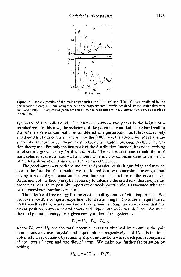
Statistical surface physics 1145
0.0 2 .o 4.0 Distance, zlo
Figure 18. Density profiles of the melt neighbouring the (111) ( a ) and (100) ( b ) faces predicted by the perturbation theory (-) and compared with the ‘experimental’ profile obtained by molecular dynamics simulation (0). The crystalline peak, around z = 0, has been fitted with a Gaussian function, as described in the text.
symmetry of the bulk liquid. The distance between two peaks is the height of a tetrahedron. In this case, the switching of the potential from that of the hard wall to that of the soft wall can really be considered as a perturbation as it introduces only small modifications of the structure. For the (100) face, the adsorption sites have the shape of octahedra, which do not exist in the dense random packing. As the perturba- tion theory modifies only the first peak of the distribution function, it is not surprising to observe a good fit only for this first peak. The subsequent ones remain those of hard spheres against a hard wall and keep a periodicity corresponding to the height of a tetrahedron when it should be that of an octahedron.
The good agreement with the molecular dynamics results is gratifying and may be due to the fact that the function we considered is a two-dimensional average, thus having a weak dependence on the two-dimensional structure of the crystal face. Refinement of the theory may be necessary to calculate the interfacial thermodynamic properties because of possibly important entropic contributions associated with the two-dimensional interface structure.
The interfacial free energy for the crystal-melt system is of vital importance. We propose a possible computer experiment for determining it. Consider an equilibrated crystal-melt system, where we know from previous computer simulations that the planar position between crystal atoms and ‘liquid’ atoms is well defined. We write the total potential energy for a given configuration of the system as
UT = UC + UL + UL-c
where Uc and UL are the total potential energies obtained by summing the pair interactions only over ‘crystal’ and ‘liquid’ atoms, respectively, and ULWc is the total potential energy obtained by summing all pair interactions where each pair is comprised of one ‘crystal’ atom and one ‘liquid’ atom. We make one further factorisation by writing
u P c = Au& + U:!&

1146 F F Abraham
where the attractive and repulsive contributions to are considered separately and the parameter A is unity for the equilibrium system. If we choose to set A = O and re-equilibrate the system, we would find that the liquid film would displace away from the crystal face and establish a liquid-vapour interface next to the crystal wall. To guarantee that the system maintains a triple-point pressure, the original liquid slab should neighbour the crystal phase at only one face, and the other face should be equilibrated with its saturated vapour phase. We can calculate the reversible work done in going from the crystal-liquid-vapour system to the crystal-vapour-liquid- vapour system by slowly reducing A from ucity to zero, equilibrating at each stage of the reduction. Since we know the interfacial free energies between liquid-vapour and crystal-vapour we can determine the crystal-liquid interfacial free energy.
6. Two-dimensional simple films
Phase transformation phenomena for ‘quasi’-two-dimensional phases adsorbed on solid surfaces has become an area of intense research activity over the last several years, the challenge being both experimental and theoretical. The systems of interest range from rare-gas atoms physisorbed on graphite (Vilcher 1980) and electrons confined to the liquid-helium surface (Grimes and Adams 1979), to polystyrene spheres trapped at the air-water interface (Pieranski 1980). We will consider some particular aspects of a strictly two-dimensional universe; the phases of matter, their transitions and solid-state stability of a system of Lennard-Jones atoms as determined by computer simulation experiments (Abraham 1980b, 1981a, b, Barker et a1 1981). This system may be considered a prototype for rare-gas-atom monolayer films on graphite. Par- ticular emphasis will centre around the low-pressure melting regime of the phase diagram. This is because of the current interest in the dislocation model of melting. Kosterlitz and Thouless (1972), and independently Feynman (Elgia and Goodstein 1974), pioneered the application of the dislocation model of melting for a two- dimensional crystal. From this theory of melting, the Kosterlitz-Thouless-Feynman criterion for the stability of a solid phase against the formation of isolated dislocations was obtained:
where T,,, is the Kosterlitz-Thouless-Feynman melting transition temperature, a is the lattice constant and p, A are the Lam6 elastic coefficients. Hence, theory predicts that K shows a universal discontinuity at the melting transition of 1 6 ~ . Furthermore, if one accepts the model that the mechanism for melting is the unbinding of a dilute gas of dislocation pairs, then this phase transition should not depend on the type of interatomic interaction. Expanding on the studies of Kosterlitz-Thouless-Feynman, Halperin and Nelson (1978) developed a detailed theory of defect-mediated melting for a two-dimensional crystal. This entailed the assumption that a ‘liquid’ close to its freezing point has a structure similar to that of a solid, but that its equilibrium configurations has some concentration of defects (dislocations and/or disclinations) to give the state liquid-like properties, i.e. in order to extend the predictions of the earlier studies, Halperin and Nelson modelled the equilibrium liquid state as a solid with particular types of topological defects. One important feature of the Halperin-

Statistical surface physics 1147
Nelson theory is the possibility that the transition from two-dimensional solid to two-dimensional liquid takes place by two second-order transitions with increasing temperature. At some temperature T , given by equation (6.1) the dissociation of dislocation pairs gives rise to a second-order transition from a solid phase, with algebraic decay of translational order and long-range orientational order, to a liquid- crystal (hexatic) phase, with exponential decay of translational order but algebraic decay of six-fold orientational order. At a higher temperature, Ti > Tm, dissociation of dislocations into disclinations gives rise to another second-order phase transition f roh the hexatic phase to the isotropic fluid phase. Halperin and Nelson do emphasise that this particular melting mechanism is only one possibility. They cannot rule out the possibility of a first-order melting transition.
Direct experimental verification of the Halperin-Nelson theory for two- dimensional melting is difficult because several possible mechanisms are involved in real systems which might conceivably influence the apparent order of the transition, e.g. epitaxy, second-layer promotion and heterogeneity, as well as the details of the adatom and substrate interactions. In order to circumvent the uncertainties and limitations of current laboratory experiments, a computer experiment may be performed on the well-defined model systems constrained to remain two-dimensional, and we will present the outcome of such experiments.
6.1. The phase diagram of two-dimensional Lennard-Jonesium
In order to construct the phase diagram for two-dimensional Lennard-Jonesium, we must calculate the free energy for the various phases as a function of the relevant intensive thermodynamic variables. We accomplished this by using two different approaches: (i) the theoretical approach by using liquid-state perturbation theory to describe the fluid phase and an approximate self-consistent cell theory to describe the solid phase, and (ii) the ‘experimental’ approach by using experimental data from isobaric-isothermal and isodensity-isothermal Monte Carlo simulations. The first approach was necessary in order that we could confine our computer experiments to the ‘interesting or questionable’ parts of the phase diagram and could minimise the computer time. The results are presented in figure 19 using both approaches. It need only be stated that the phase diagrams resulting from the two different methods were essentially the same. We make special note of the fact that only three phases of two-dimensional matter appear on these phase diagrams-solid, liquid and vapour. This is not unexpected from the theoretical approach since the two theories employed-the self-consistent cell theory and the liquid-state perturbation theory- explicitly describe only the crystal and fluid phases of matter, and no theoretical account is made for the possibility of a distinctly different phase of matter, such as the proposed hexatic phase. The reality of the various phases of two-dimensional matter can only be ascertained by experiments. We now describe the computer experiments.
6.2. Monte Carlo and molecular dynamics experiments
6.2.1. The isobaric-isothermal Monte Carlo simulations. The (N, P, T) Monte Carlo calculations were performed on N = 256 and 529 atom systems with periodic boundary conditions to simulate: the bulk. In a typical simulation ‘experiment’, the system was initialised using an equilibrium configuration at a neighbouring temperature and

1148 F F Abraham
0.3 0.4 0.5 0.6 0 0.5 1.0 Temperature, k T/E Density, p u2
Figure 19. (a) Phase diagram in the pressure-temperature plane for the two-dimensional Lennard-Jones system. The full curves are predicted using liquid-state perturbation theory and the self-consistent cell model for the solid state. The broken curves are obtained by interpolation using Monte Carlo experimental data. ( b ) Phase diagram in the density-temperature plane for the two-dimensional Lennard-Jones system. The full curves are predicted using liquid-state perturbation theory and the self-consistent cell model for the solid state. The phase diagram obtained by interpolation using Monte Carlo experimental data agrees very well with this diagram.
‘equilibrated’ through Ne Monte Carlo moves with a 50% acceptance ratio. Each move is comprised of an atomic displacement and an area scaling. After equilibration, N , further moves were performed to obtain the enthalpy H, the average density p , the pair distribution function g ( r ) , and other quantities, the total number of moves being greater near the melting transition and in the liquid region. For the 256-atom system, Ne and N , equalled lo6 and 2-6 x lo6 configurations, respectively. For the 529-atom system, Ne and N , equalled 2 x lo6 and 9 x lo6 configurations, respectively. Careful attention was given to determine that the system was in ‘local equilibrium’ (stable or metastable) when taking the statistics for the quantities of interest, i.e. the distribution and running mean of density, enthalpy and viral pressure were monitored.
In figure 20, we present the equilibrium density p* = p u 2 and the enthalpy per atom h” = H / N E for the Lennard-Jones system of 256 atoms as a function of tem- perature T* = kT/E and for a fixed pressure P* = Pa2/€ = 0.01, 0.05 and 1.0, respec- tively. The first two pressures were intentionally chosen to be low since Nelson and Halperin have speculated that the melting transition could be first order at high pressures but second order at low pressures, and since it was suggested that earlier studies were examining a high-(temperature, density) regime where melting becomes first order. Considering first the density behaviour at P* = 0.05, we note that the solid density decreases smoothly as the temperature is sequentially increased and the system is equilibrated up to the temperature T* = 0.46. From T* = 0.40 to 0.45, 4 x lo6 equilibrium configurations are generated at each temperature. At T* = 0.46, the solid melts into a liquid with a dramatic decrease in equilibrium density p : - p ? = 0.11.
The pair distribution functions and ‘snapshot’ pictures of the atomic configurations (see figures 21 and 22) show the change from crystalline order to liquid disorder. At higher temperatures, the liquid density decreases smoothly. By sequential decrease

Statistical surface physics 1149
0.8
0.7
& 0.6
2 0.5 0"
0.022
0.020
N
2, c
- -4.0
~ -3.0
--2.0
0.6 I 0.4 0.5 0.6 0.2 0.3 0.4 0.5 0.50 0.55 0.60
Temperature, k T / c
Figure 20. The equilibrium density and enthalpy per atom as a function of temperature for a Lennard-Jones system at fixed pressures P* = 0.01 (a ) , 0.05 ( b ) and 1.0 ( c ) . Note that at P* = 0.01, the system both melts and vaporises. The inserted data at P* = 1.0 are taken from Toxvaerd (1978).
t I
4 8 r l a
0 4 8
Figure 21. The pair distribution function of the Lennard-Jones system at T* = 0.45 when it is a solid ( a ) and a liquid ( b ) .
of temperature and equilibration, the system passes through T" = 0.46 and remains a liquid with smoothly increasing density down to a temperature T" = 0.43 (again, the pair distribution functions reflect the fact that the undercooled states are liquid). This establishes hysteresis when passing back through the apparent melting tem- perature. At T* = 0.4, the liquid solidifies with a sharp increase in density p $ = 0.8; however, this density is lower than the original solid density at that temperature, p $ =0.85. Examination of the atomic structure of this solid, which was nucleated from the liquid phase, revealed significant defect structure which accounts for the density difference for the two solid systems. Of course, it would be unlikely that the supercooled liquid would solidify directly into a defect-free crystal structure. We also note in figure 20 that the enthalpy of the system has the same behaviour as the density and yields a latent heat of -0.44~/atom.
Similar features are seen in figure 20 for the low pressure of P* = 0.01 and for the high pressure of P" = 1.0, It is particularly interesting to note that the low-pressure
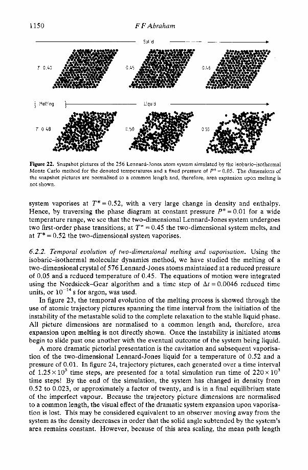
1150 F F Abraham
Solid b
Melting 1- Liquid b
T 0 .48
Figure 22. Snapshot pictures of the 256 Lennard-Jones atom system simulated by the isobaric-isothermal Monte Carlo method for the denoted temperatures and a fixed pressure of P* = 0.05. The dimensions of the snapshot pictures are normalised to a common length and, therefore, area expansion upon melting is not shown.
system vaporises at T * = 0.52, with a very large change in density and enthalpy. Hence, by traversing the phase diagram at constant pressure P* = 0.01 for a wide temperature range, we see that the two-dimensional Lennard-Jones system undergoes two first-order phase transitions; at T * = 0.45 the two-dimensional system melts, and at T * = 0.52 the two-dimensional system vaporises.
6.2.2. Temporal evolution of two-dimensional melting and vaporisation. Using the isobaric-isothermal molecular dynamics method, we have studied the melting of a two-dimensional crystal of 576 Lennard-Jones atoms maintained at a reduced pressure of 0.05 and a reduced temperature of 0.45. The equations of motion were integrated using the Nordsieck-Gear algorithm and a time step of At = 0.0046 reduced time units, or
In figure 23, the temporal evolution of the melting process is showed through the use of atomic trajectory pictures spanning the time interval from the initiation of the instability of the metastable solid to the complete relaxation to the stable liquid phase. All picture dimensions are normalised to a common length and, therefore, area expansion upon melting is not directly shown. Once the instability is initiated atoms begin to slide past one another with the eventual outcome of the system being liquid.
A more dramatic pictorial presentation is the cavitation and subsequent vaporisa- tion of the two-dimensional Lennard-Jones liquid for a temperature of 0.52 and a pressure of 0.01. In figure 24, trajectory pictures, each generated over a time interval of 1.25 x lo3 time steps, are presented for a total simulation run time of 220 x lo3 time steps! By the end of the simulation, the system has changed in density from 0.52 to 0.023, or approximately a factor of twenty, and is in a final equilibrium state of the imperfect vapour. Because the trajectory picture dimensions are normalised to a common length, the visual effect of the dramatic system expansion upon vaporisa- tion is lost. This may be considered equivalent to an observer moving away from the system as the density decreases in order that the solid angle subtended by the system’s area remains constant. However, because of this area scaling, the mean path length
s for argon, was used.

Statistical surface physics 1151
Figure 23. Atomic trajectory pictures showing the melting of a two-dimensional Lennard-Jones solid of 576 atoms at (P*, T*) = (0.05,0.45). These trajectories depict the temporal evolution of the melting process as observed from the isobaric-isothermal molecular dynamics method. Time is in number of time steps. The two centred boxes in the upper left-hand corner of each picture of figure 23 show the instantaneous area of the system (inner box) relative to the final area of the equilibrium liquid (outer box). In the case of melting, the boxes differ very little in size.
of a vapour atom in the low-density phase appears much shorter than the mean path length of a comparable-type atom in the early-time, high-density phase. In an attempt to graphically depict this expansion, the two centred boxes in the upper left-hand corner of each picture in figure 24 show the instantaneous area of the system (inner box) relative to the final area of the equilibrium vapour (outer box). Only by doing a constant pressure experiment could we have simulated the transition dynamics of a phase change from a condensed-phase density to a vapour-phase density, such a simulation study being impossible if the mean density was constrained to be constant.
6.2.3. The phase diagram revisited. The phase diagram has been accurately calculated by interpolation of Monte Carlo experimental data for a two-dimensional Lennard- Jones system of 256 atoms with periodic boundary conditions. For each calculation at least 1.2 x lo6 configurations (with an acceptance ratio close to 0.5) were used to calculate averages and 0.35 x lo6 configurations to approach equilibration; in the two-phase region several times as many configurations were used.
To determine the Helmholtz free energy F and chemical potential CL which are required for locating phase boundaries, the equations
af*/ap* = P * / P * ~ (6.2) and

1152 F F Abraham
20000 ..._
I
220000 r-7
Figure 24. Atomic trajectory pictures showing the vaporisation of a two-dimensional Lennard-Jones liquid of 576 atoms at (P*, T*) = (0.01,0.52). Like all previous trajectory pictures, the picture dimensions are normalised to a common length and, therefore, area expansion is not shown. This is equivalent to an observer moving away from the system as the density decreases in order that the solid angle subtended by the system's area remains constant. However, the two centred boxes in the upper left-hand corner of each picture in figure 24 show the instantaneous area of the system (inner box) relative to the final area of the equilibrium vapour (outer box).
have been integrated along appropriate reversible paths in the (p, T ) plane joining reference thermodynamic states, for which the free energy is known. In equations (6.2) and (6.3) f*=F/NE and U * = U/NE. For fluid states the most convenient reference state is zero density at a particular temperature which was chosen at T* = 1.0. The solid-state reference state was taken at T* = 0.0, p * = 0.9165. In the neighbour- hood of T" = 0, the classical solid behaves as a purely harmonic crystal for which the free energy can be calculated by standard methods of lattice dynamics. The density p * = 0.9165 lies outside the two-phase region for all the temperatures studied so that there is no problem with reversibility. At the lowest temperature the fluid path lies in the liquid-vapour two-phase region. In this range, a constraint was imposed to ensure that phase separation would not occur. Since this constraint was used only in a high-density region it should not lead to serious error. The details of the free energy determination for the various phases is described in Barker et al (1981) and will not be repeated here.
From the fact that the chemical potential is given by
p * = f* + P*/p* (6.4)
the phase coexistence was determined by solving the simultaneous equations
(6.5)
P k i d = P:olid. (6.6)
* * CL fluid = solid
Statistical surface physics 1153
This is equivalent to constructing common tangents to solid and fluid free energy/area curves (for the constant density calculations) or to locating crossings of p * / T " curves (for constant pressure calculations).
From figure 19, we note that the agreement between the phase diagram calculated from theory and from the Monte Carlo results is really quite striking. This free energy construction of the phase diagram supports the conclusion that the hexatic phase is non-existent and that melting in two dimensions is first order for the Lennard-Jones 12 : 6 system.
6.2.4. The Kosterlitz-Thouless-Feynman criterion and its relation to melting : a very important result. We have presented an isobaric-isothermal Monte Carlo computer simulation study on melting for a two-dimensional Lennard-Jones system and conclude that the melting transition is first order, in contrast to the two-stage, second-order melting behaviour suggested as a possibility by Halperin and Nelson. We now show that the Kosterlitz-Thouless-Feynman instability criterion for a two-dimensional solid (equation (6.1)) is satisfied at the observed first-order melting transition for the Monte Carlo and molecular dynamics experiments. This is inconsistent with renormalisation group arguments of Halperin and Nelson that the transition should be continuous. Finaiiy, the suggestion that the computer experiments may have missed the hexatic phase because of critical slowing down of the relaxation processes near the alleged second-order melting transition is not supported by these findings, since the observed melting temperature equals the Kosterlitz-Thouless-Feynman instability temperature, and this instability temperature is significantly greater than the thermodynamic melting temperature.
From the dislocation model of melting for a two-dimensional solid, the Kosterlitz- Thouless-Feynman (KTF) criterion for the stability of a solid phase against the formation of isolated dislocations was found to be given by equation (6.1). Hence, the parameter K shows a universal discontinuity of 1 6 ~ at the instability temperature which Kosterlitz-Thouless and Halperin-Nelson identify with the thermodynamic melting temperature. The point of view argued here is that the metastable solid does indeed become unstable at this temperature but that this bears no relation to the thermodynamic melting transition; the dislocation-unbinding instability provides a path by which the system reaches the stable (liquid) phase which becomes the thermodynamic stable phase at a lower temperature.
The studies on two-dimensional melting of a Lennard-Jones solid have been extended by calculating numerically the Lam6 coefficients as a function of temperature and density (Abraham 1981a). For the 529 Lennard-Jones atom system at fixed temperatures and densities corresponding to an average pressure of P* = 0.05, we have calculated the Lam6 coefficients. From the measured Lam6 coefficients and equation (6. l), the Kosterlitz-Thouless parameter K was obtained and is presented as a function of temperature in figure 25. We note that at the observed instability temperature T ; = 0.45, K has approached, by extrapolation, the approximate value of 1 6 ~ , while at the neighbouring temperature of 0.44 the K of the solid is significantly above 167~. Using the experimental elastic constant data for temperatures below 0.45, we estimate that the instability temperature based on the Kosterlitz-Thouless- Feynman criterion is 0.45 f 0.005. The measured value of K at the observed melting temperature is significantly lower than 1 6 ~ because of defect formation in the solid constrained to remain at a solid density. We conclude that this experimentally observed melting temperature is consistent with the Kosterlitz-Thouless-Feynman instability

1154 F F Abraham
0.40 0.44 0.48
I 0 40 0 42 0 44
Temperature , ~ T / E
Figure 25. The Kosterlitz-Thouless parameter K as a function of temperature for the 529 Lennard-Jones atom system at fixed temperatures and densities corresponding to an average pressure of P* = 0.05. The density variation is shown in ( a ) .
criterion and that the transition at this temperature is consistent with a first-order phase change. This first-order behaviour contradicts the prediction based on the application of renormalisation group arguments to the dislocation for melting where it is predicted that the two-dimensional melting transition is continuous.
The detailed free energy analyses yielding the phase diagram of the two- dimensional Lennard-Jones system finds that the thermodynamic melting temperature is approximately 0.415. This is in sharp contrast to the finding that computer experi- ment and the Kosterlitz-Thouless-Feynman theory give a melting temperature of -0.45. However, this may be resolved by the following argument. The dislocation theory of melting only describes the stability of the solid state in terms of the improbable existence of solid-state defects (e.g. dislocations, declinations) in its equilibrium solid structure. At the Kosterlitz-Thouless-Feynman instability temperature, a dilute con- centration of defects becomes likely and the solid may then readily transform to the lowest free energy phase, the liquid state. Certainly, the defect solid with a low concentration of dislocations is not a proper model for a liquid and must be in a higher free energy state relative to the equilibrium liquid state. However, the defect solid state is an effective precursor for melting to the liquid state. In the laboratory, atomic solids do not melt at this stability limit to defect formation, but melt at, or very near to, their thermodynamic melting temperature. This is because of the necessary existence of a solid surface. In figure 26, this is demonstrated by Monte Carlo simulations of a two-dimensional strip of 512 Lennard-Jones atoms at a temperature (0.40) slightly below and at a temperature (0.42) slightly above the thermodynamic melting temperature of 0.415 and initialised at the appropriate

Statistical surface physics 1155
low-pressure, solid-state densities for the respective temperatures. Periodic boundary conditions exist at the strip’s horizontal boundaries, while the two vertical boundaries are free surfaces in contact with a vapour-phase region. The trajectory plots are generated from 5 x lo6 consecutive configurations and are typical of the equilibrium atomic behaviour of the strip over a continuous simulation of -50 x lo6 configurations for each temperature. The simulations clearly demonstrate a stable crystal phase with premelted surfaces at T* = 0.40 (figure 26(a) ) and a stable liquid phase at T* = 0.42 (figure 26(b)). The results in figure 26(b) also provided nice confirmation that the estimate of the thermodynamic melting temperature from free energy considerations is valid. In the computer experiments, it is easy (actually, too easy) to exclude the presence of surfaces by imposing periodic conditions at all boundaries of the computa- tional cell and to effectively constrain the solid to superheat well beyond the thermody- namic melting temperature.
Figure 26. Atomic trajectory pictures of a two-dimensional Lennard-Jones system of 512 atoms with two free surfaces for a temperature 0.40 slightly below ( a ) and a temperature 0.42 slightly above ( b ) the thermodynamic melting point of 0.415.
We may imagine other types of fluctuations that may result in a different stability limit for the ‘surfaceless’ atomic solid. For example, in a heterophase fluctuation, we would consider a local crystal region of a few tens of atoms which would ‘melt’ (i.e. a liquid cluster embedded in the crystal matrix). However, because of the density difference between the liquid and solid states and because of liquid layering neighbour- ing a crystal boundary, the energetics would be prohibitive, and this heterophase precursor to melting would be very unlikely. We conclude that the dislocation- dissociation mechanism is the most efficient precursor to bulk melting of the metastable solid.

1156 F F Abraham
In summary, the dislocation-unbinding model for two-dimensional melting leads to a theoretical instability temperature that is consistent with the experimentally observed instability temperature of the solid phase. However, this melting temperature is not the thermodynamic melting temperature, this being much lower; it is a tem- perature corresponding to an upper limit for the stability of the metastable, two- dimensional solid with no free surfaces. Also, the renormalisation group arguments applied to the Kosterlitz-Thouless-Feynman model predict that the melting transition is continuous, in sharp contrast to the first-order character observed in the computer experiments. We conclude that the dislocation-unbinding theory for melting does not give a correct thermodynamic theory of melting. The thermodynamic melting tem- perature is sigcificantly lower than the temperature for which the solid becomes unstable to dislocation pair dissociation (the Kosterlitz-Thouless-Feynman tem- perature), and the thermodynamic phase transition is first-order.
It seems likely that these findings and conclusions for the melting of a two- dimensional atomic solid are also valid for three dimensions.
6.3. Comment on isodensity-isothermal simulations
We will comment on studying a first-order melting transition by using molecular dynamics (Frenkel and McTague 1979) or Monte Carlo (Tobochnick and Chester 1980) where the number of particles, the area, and hence the density, is constrained to remain constant. In figure 27, the dependence of the pressure, heat capacity and energy on temperature is shown, assuming equilibrium as the system passes through the two-phase region. We note that these features were observed in the fixed density molecular dynamics and Monte Carlo experiments, but the investigators interpreted the experiments as evidence for two consecutive second-order melting transitions. Employing the constant density (N, A, T ) Monte Carlo method, we have calculated the equation of state for Lennard-Jonesium at a reduced density of 0.84. Briefly, we see features of the (P, T ) equation of state consistent with figure 27. In figure 28 (before) a trajectory plot of the 256 atom over 1.4 x lo6 configurations is presented for the reduced temperature of 0.7, this density/temperature position being bounded
T w o - phase region
Two - phase region
Temperature, T -+
Figure 27. The dependence of pressure, heat capacity and energy on temperature as a constant density system in equilibrium passes through the two-phase (solid-liquid) region.

Statistical surface physics 1157
Before After
Figure 28. ‘Before’ is the constant density simulation at T* = 0.7, p* = 0.84 and mean pressure (P*) = 2.55. ‘After’ is obtained by starting from a configuration of ‘before’ and performing a constant pressure experiment at the same temperature T* = 0.7 and pressure P* = 2.55. The system becomes entirely crystalline with a density equal to 0.867.
by the two ‘kinks’ in the (P, T ) equation of state. From this trajectory plot, a reasonable interpretation is that the system is in the two-phase, solid-liquid region and that invoking the existence of a new phase (e.g. the hexatic phase) is not needed. Also, Tobochnick and Chesters’ observation that K = 1 6 ~ at melting is consistent with the transition being first order. We did one further experiment. Starting with a configur- ation consistent with two-dimensional solid-liquid coexistence obtained using the ( N , A , T ) Monte Carlo method (figure 28 (before)), we did a constant pressure- temperature experiment using a pressure equal to the mean pressure of the two-phase system and at the same temperature. The system immediately relaxed to the crystalline state with a density p* = 0.867. This shows that (i) the ‘before’ state in figure 28 is not the lowest free energy state and (ii) that it is not difficult to crystallise to a perfect solid from the two-phase region.
An obvious next step is to study by computer simulation the phases of quasi-two- dimensional systems, such as submonolayer physisorbed atoms or molecules on well- characterised crystalline substrates-the classic examples being the rare gases on graphite. The richness, complexity and importance of newly emerging surface phenomena has captured the interest of researchers spanning a wide spectrum of traditional disciplines, and computer simulation will continue to play a very important role in the resolution of outstanding issues of current and future interest in this field.
Acknowledgments
The author has benefited greatly from discussions and active collaborations with several of his colleagues while at the IBM San Jose Research Laboratory, in particular John Barker, Alain Bonissent (CNRS, Marseille), Jeremy Broughton (Bell Laboratories), Rashmi Desai (Toronto), Doug Henderson, Bill Hoover (Lawrence Livermore Laboratory), Stefan Koch (Frankfurt), William Rudge and Mark Warner (Rutherford Laboratory, England). A special ‘thank you’ goes to Blanca Gallegos and Lorraine Candelaria for typing the manuscript.

1158 F F Abraham
Referencest
Abraham F F 1974 Homogeneous Nucleation Theory (New York: Academic) - 1978 J. Chem. Phys. 68 3713 __ 1979 Phys. Rep. 53 93 - 1980a J. Chem. Phys. 72 1412 - 1980b Phys. Rev. Lett. 44 463 - 1981a Phys. Rev. B 23 6145 - 1981b Phys. Rep. 80 339 Abraham F F, Schreiber D E and Barker J A 1975 J. Chem. Phys. 62 1958 Abraham F F and Singh Y 1977 J. Chem. Phys. 67 2384 Andersen H C 1980 J. Chem. Phys. 72 2384 Andersen H C, Weeks .I D and Chandler D 1971 Phys. Rev. A 4 1597 Band W 1939 J. Chem. Phys. 7 324 Barker J A and Henderson D 1976 Rev. Mod. Phys. 48 587 Barker J A, Henderson D and Abraham F F 1981 Physica 106A 226 Beaglehole D 1979 Phys. Rev. Lett. 43 2016 Becker R and Doring W 1935 Ann. Phys., Lpz. 24 710 Bernal J D 1959 Nature 183 141 - 1964 Proc. R . Soc. A 280 299 Bijl A 1938 Discontinuities in the Energy and Specific Heat. Doctoral Dissertation Leiden Bonissent A and Abraham F F 1981 J. Chem. Phys. 74 1306 Broughton J Q and Abraham F F 1980 Chem. Phys. Lett. 71 456 Broughton J Q, Bonissent A and Abraham F F 1981 J. Chem. Phys. 74 4029 Buff F P, Lovett R A and Stillinger F H 1965 Phys. Rev. Lett. 15 621 Cahn J W 1961 Acta Metall. 9 795 Cahn J W and Hilliard J E 1958 J . Chem. Phys. 28 258 - 1959 J. Chem. Phys. 31 688 Chapela G A, Saville A, Thompson S M and Rowlinson J S 1977 J. Chem. Soc. Faraday Trans. IZ 73 1133 Elgin R L and Goodstein D L 1974 Phys. Rev. A 9 2657 Finney J L 1970 Proc. R. Soc. A 319 479, 495 Fisk S and Widom B 1969 J. Chem. Phys. 50 3219 Frenkel D and McTague J P 1979 Phys. Rev. Lett. 42 1632 Frenkel J 1939 J . Chem. Phys. 7 538 Garcia N G and Torroja J M S 1981 Phys. Rev. Lett. 47 186 Gear C W 1966 Argonne National Laboratory Rep. ANL-7126 Grimes C C and Adams G 1979 Phys. Rev. Lett. 42 795 Halperin B I and Nelson D R 1978 Phys. Rev. Letr. 41 121, 519(E) Hill T L 1955 J. Chem. Phys. 23 812 Kosterlitz J M and Thouless D J 1972 Solid St. Phys. 5 L124 Ladd A J C and Woodcock L V 1978a Molec. Phys. 36 611 - 1978b J. Phys. C: Solid St. Phys. 11 3565 Lee J K, Barker J A and Abraham F F 1973 J. Chem. Phys. 58 3166 Lee J K, Barker J A and Pound G M 1974 J. Chem. Phys. 60 1976 Lothe J and Pound G M 1962 J. Chem. Phys. 36 2080 Mayer J E 1937 J. Chem. Phys. 5 67 Metropolis N, Rosenbluth A W, Rosenbluth M N, Teller A H and Teller E 1953 J. Chem. Phys. 21 1087 Nordsieck A 1962 Math. Comput. 16 22 Pieranski P 1980 Phys. Rev. Lett. 45 569 Rahman A 1964 Phys. Rev. 136 A405 Rowlinson J S 1979 J. Stat. Phys. 20 197 Singh Y and Abraham F F 1977 J. Chem. Phys. 67 537 Stranski I N 1942 Naturw. 30 425 Tobochnick J and Chester G V 1980 Ordering In Two Dimensions ed S K Sinha (Amsterdam: North-
Holland) p 339
t The reader should note that a bibliography providing a limited survey of the various topics discussed in this paper follows the references.

Statistical surface physics 1159
Toxvaerd S 1978 J. Chem. Phys. 69 4750 van der Waals J D 1893 Verh. K. Akad. Wet. Amsterdam Section 1 l(8) Vilcher 0 E 1980 Ann. Rev. Phys. Chem. 31 463 Woodruff D P 1973 The Solid-Liquid Interface (Cambridge: Cambridge University Press)
Computer simulations in surface science: an incomplete bibliography
( a ) General treatises on statistical physics of surfaces Buff F P 1960 Handb. Phys. 10 281-304 Croxton C A 1980 Statistical Mechanics Of The Liquid Surface (New York: Wiley) Dash J G 1975 Films On Solid Surfaces (Oxford: Pergamon) Defay R, Prigogine I, Bellemans A and Everett D H 1966 Surface Tension And Adsorption (New York:
Ono S and Kondo S 1960 Handb. Phys. 10 134-280 Rowlinson J S 1979 J. Stat. Phys. 20 197 Rowlinson J S and Widom B 1982 Molecular Theory Of Capillarity (Oxford: Oxford University Press) to
Steele W A 1974 The Interaction Of Gases With Solid Surfaces (Oxford: Pergamon)
( b ) General descriptions of computer simulation methods Alder B J and Hoover W G 1968 Physics of Simple Liquids ed H N V Temperley, J S Rowlinson and G
S Rushbrooke (Amsterdam: North-Holland) chap 4 Binder K (ed) 1979 Monte Carlo Methods In Statistical Physics (Berlin: Springer-Verlag) Erpenbeck J J and Wood W W 1977 StatisticalMechanics Part B: Time-Dependent Processes ed B J Berne
Kushick J and Berne B J 1977 Statistical Mechanics Part B: Time-Dependent Processes ed B J Berne (New
Hockney R W and Eastwood J W 1981 Computer Simulation Using Particles (New York: McGraw-Hill) Levesque D, Weis J-J and Hansen J-P 1979 Monte Carlo Methods in Statistical Physics ed K Binder (Berlin:
Valleau J P and Torrie G 1977 Statistical Mechanics Part A: Equilibrium Techniques ed B J Berne (New
Valleau J P and Whittington S 1977 Statistical Mechanics Part A: Equilibrium Techniques ed B J Berne
Wood W W 1968 Physics of Simple Liquids ed H N V Temperley, J S Rowlinson and G S Rushbrooke
Wiley)
appear
(New York: Plenum) chap 1
York: Plenum) chap 2
Springer-Verlag) chap 2
York: Plenum) chap 5
(New York: Plenum) chap 4
(Amsterdam: North-Holland) chap 5
( c ) Microclusters of simple systems Abraham F F 1974 Homogeneous Nucleation Theory (New York: Academic) - 1974 J. Chem. Phys. 61 1221 Abraham F F and Barker J A 1975 J . Chem. Phys. 63 2266 Abraham F F, Mruzik M R and Pound G M 1976 Faraday Discuss. Chem. Soc. 61 34 Binder K and Kalos M H 1980 J~ Stat. Phys. 22 363 Bonissent A and Mutaftschiev B 1974 J . Cryst. Growth 24/25 503 Briant C L and Burton J J 1973 Nature 243 100 - 1975 J. Chem. Phys. 63 2045 - 1975 J. Chem. Phys. 63 3327 - 1976 J. Chem. Phys. 64 2888 Dickey J M and Paskin A 1970 Phys. Rev. B 1 851 Garcia Garcia N and Soler Torroja J M 1981 Phys. Rev. Lett. 47 186 Kristensen W D, Jensen E J and Cotterill R M J 1974 J. Chem. Phys. 60 4161 Lee J K, Barker J A and Abraham F F 1973 J. Chem. Phys. 58 3166 McGinty D J 1973 J. Chem. Phys. 58 4733 Miyazaki J, Pound G M, Abraham F F and Barker J A 1977 J. Chem. Phys. 67 3851 Mruzik M R 1977 Chem. Phys. Lett. 48 171 Mruzik M R, Abraham F F, Schreiber D E and Pound G M 1976 J. Chem. Phys. 64 481

1160 F F Abraham
Rao M, Berne B J and Kalos M H 1978 J. Chem. Phys. 68 1325 Swope W C, Andersen H C, Berens P H and Wilson K R 1981 J. Chem. Phys. 76 637 Tsai N-H, Abraham F F and Pound G M 1978 Surf. Sci. 77 465
( d ) The liquid-vapour interface Abraham F F 1980 J. Chem. Phys. 72 1412 Abraham F F, Schreiber D E and Barker J A 1975 J. Chem. Phys. 62 1958 Chapela G A, Saville G and Rowlinson J S 1975 Faraday Discuss. Chem. Soc. 59 22 Chapela G A, Saville G, Thompson S M and Rowlinson J S 1977 Faraday Discuss. Chem. Soc. 73 1133 Croxton C A and Ferrier R P 1971 J. Phys. C: Solid St. Phys. 4 2447 Gubbins K E and Thompson S M 1981 J. Chem. Phys. 74 6467 Kalos M H, Percus J K and Rao M 1977 J. Stat. Phys. 17 111 Lee C Y and Scott H L 1980 J. Chem. Phys. 73 4591 Lee J K, Barker J A and Pound G M 1974 J. Chem. Phys. 60 1976 Liu K S 1974 J. Chem. Phys. 60 4226 Opitz A C L 1974 Phys. Lett. 47A 439 Rao M and Berne B J 1979 Molec. Phys. 37 455 Rao M and Levesque D 1976 J. Chem. Phys. 65 3233 Thompson S M 1978 Faraday Discuss. Chem. Soc. 66 107 Thompson S M and Gubbins K E 1979 J. Chem. Phys. 70 4947 Toxvaerd S 1975 J. Chem. Phys. 62 1589
( e ) The solid-liquid interface Abraham F F 1978 J. Chem. Phys. 68 3713 - 1981 Phys. Rev. B 23 6145 Abraham F F and Singh Y 1977 J. Chem. Phys. 67 2384 - 1978 J. Chem. Phys. 68 4767 Abraham F F, Tsai N-H and Pound G M 1978 Surf. Sci. 78 181 Bonissent A and Abraham F F 1981 J. Chem. Phys. 74 1306 Bonissent A, Gauthier E and Finney J L 1979 Phil. Mag. B 39 49 Broughton J Q and Abraham F F 1980 Chem. Phys. Lett. 71 456 Broughton J Q, Bonissent A and Abraham F F 1981 J. Chem. Phys. 74 4029 Broughton J Q and Woodcock L V 1978 J. Phys. C: Solid St. Phys. 11 2743 Cape J N 1982 J. Chem. Soc. Faraday Trans. 2 78 317 Chapela G A, Saville G and Rowlinson J S 1975 Faraday Discuss. Chem. Soc. 59 22 (while the authors
were primarily interested in the liquid-vapour interface, they stabilised the fluid slab with a Lennard- Jones 9-3 wall potential and, therefore, did one of the first solid-liquid interface simulations)
Hiwatari Y , Stoll E and Schneider T 1978 J. Chem. Phys. 68 3401 Ladd A J C and Woodcock L V 1977 Chem. Phys. Lett. 51 155 - 1978 Molec. Phys. 36 611 - 1978 J. Phys. C: Solid St. Phys. 11 3565 Landman U, Cleveland C L and Brown C S 1980 Phys. Rev. Lett. 45 2032 Lane J E and Spurling T H 1979 Chem. Phys. Lett. 67 107 Rao M, Berne B J, Percus J K and Kalos M H 1979 J. Chem. Phys. 71 3802 Snook I K and Henderson D 1978 J. Chem. Phys. 68 2134 Toxvaerd S and Praestgaard E 1977 J. Chem. Phys. 67 5291
( f ) The idealised monolayer film: two -dimensional Lennard-Jones matter: see comment in Abraham (1981) Abraham F F 1980 Phys. Rev. Lett. 44 463 - 1980 Ordering In Two Dimensions ed S K Sinha (Amsterdam: North-Holland) pp 155-62 - 1981 Phys. Rev. B 23 6145 - 1981 Phys. Rep. 80 339 (the appendix has a more extensive bibliography for computer simulations
of the phases for a variety of atomic systems, e.g. hard discs, classical one-component plasma and the interfacial colloid system)
Barker J A, Henderson D and Abraham F F 1981 Physica 106A 226 Cotterill R M J and Pederson L B 1972 Solid St. Commun. 10 439 De Wette F W, Allen R E, Hughes D S and Rahman A 1969 Phys. Lett. 29A 548 Frenkel D and McTague J P 1979 Phys. Rev. Lett. 42 1632

Statistical surface physics 1161
Henderson D 1977 Molec. Phys. 34 301 McTague J P, Frenkel D and Allen M P 1980 Ordering In Two Dimensions ed S K Sinha (Amsterdam:
Phillips J M, Bruch L W and Murphy R D 1981 J. Chem. Phys. 75 5097 Tobochnik J and Chester G V 1980 Ordering In Two Dimensions ed S K Sinha (Amsterdam: North-Holland)
Toxvaerd S 1978 J. Chem. Phys. 69 4750 - 1980 Phys. Rev. Lett. 44 1002 Tsien F and Valleau J 0 1974 Molec. Phys. 27 177 Van Swol F, Woodcock L V and Cape J N 1980 J. Chem. Phys. 73 913
North-Holland) pp 147-54
pp 339-40