statistical ranking and combinatorial hodge theory
TRANSCRIPT

Noname manuscript No.(will be inserted by the editor)
Statistical ranking and combinatorial Hodge theory
Xiaoye Jiang · Lek-Heng Lim · Yuan Yao ·Yinyu Ye
Received: date / Accepted: date
Abstract We propose a technique that we call HodgeRank for ranking data thatmay be incomplete and imbalanced, characteristics common in modern datasetscoming from e-commerce and internet applications. We are primarily interestedin cardinal data based on scores or ratings though our methods also give specificinsights on ordinal data. From raw ranking data, we construct pairwise rankings,represented as edge flows on an appropriate graph. Our statistical ranking methodexploits the graph Helmholtzian, which is the graph theoretic analogue of theHelmholtz operator or vector Laplacian, in much the same way the graph Laplacianis an analogue of the Laplace operator or scalar Laplacian. We shall study the graphHelmholtzian using combinatorial Hodge theory, which provides a way to unravelranking information from edge flows. In particular, we show that every edge flowrepresenting pairwise ranking can be resolved into two orthogonal components,a gradient flow that represents the l2-optimal global ranking and a divergence-
X. Jiang acknowledges support from ARO Grant W911NF-04-R-0005 BAA and the School ofEngineering fellowship at Stanford. L.-H. Lim acknowledges support from the Gerald J. Lieber-mann fellowship at Stanford and the Charles B. Morrey assistant professorship at Berkeley.Y. Yao acknowledges support from PKU 985 project, Microsoft Research Asia, DARPA GrantHR0011-05-1-0007, and NSF Grant DMS 0354543. Y. Ye acknowledges support from AFOSRGrant FA9550-09-1-0306 and DOE Grant DE-SC0002009.
Xiaoye JiangInstitute for Computational and Mathematical Engineering, Stanford University, Stanford, CA94305, USAE-mail: [email protected]
Lek-Heng LimDepartment of Mathematics, University of California, Berkeley, CA 94720, USAE-mail: [email protected]
Yuan YaoSchool of Mathematical Sciences, Peking University and LMAM, Key Laboratory of MachinePerception, Ministry of Education, Beijing 100871, P.R. ChinaE-mail: [email protected]
Yinyu YeDepartment of Management Science and Engineering, Stanford University, Stanford, CA 94305,USAE-mail: [email protected]

2 X. Jiang, L.-H. Lim, Y. Yao, Y. Ye
free flow (cyclic) that measures the validity of the global ranking obtained — ifthis is large, then it indicates that the data does not have a good global ranking.This divergence-free flow can be further decomposed orthogonally into a curl flow(locally cyclic) and a harmonic flow (locally acyclic but globally cyclic); theseprovides information on whether inconsistency in the ranking data arises locallyor globally.
When applied to statistical ranking problems, Hodge decomposition sheds lighton whether a given dataset may be globally ranked in a meaningful way or if thedata is inherently inconsistent and thus could not have any reasonable globalranking; in the latter case it provides information on the nature of the inconsis-tencies. An obvious advantage over the NP-hardness of Kemeny optimization isthat HodgeRank may be easily computed via a linear least squares regression.We also discuss connections with well-known ordinal ranking techniques such asKemeny optimization and Borda count from social choice theory.
Keywords Statistical ranking · rank aggregation · combinatorial Hodge theory ·discrete exterior calculus · combinatorial Laplacian · graph Helmholtzian ·HodgeRank · Kemeny optimization · Borda count
Mathematics Subject Classification (2000) 68T05 · 58A14 · 90C05 · 90C27 ·91B12 · 91B14
1 Introduction
The problem of ranking in various contexts has become increasingly important inmachine learning. Many datasets1 require some form of ranking to facilitate iden-tification of important entries, extraction of principal attributes, and to performefficient search and sort operations. Modern internet and e-commerce applicationshave spurred an enormous growth in such datasets: Google’s search engine, Cite-Seer’s citation database, eBay’s feedback-reputation mechanism, Netflix’s movierecommendation system, all accumulate a large volume of data that needs to beranked.
These modern datasets typically have one or more of the following features thatrender traditional ranking methods (such as those in social choice theory) inap-plicable or ineffective: (1) unlike traditional ranking problems such as votings andtournaments, the data often contains cardinal scores instead of ordinal orderings;(2) the given data is largely incomplete with most entries missing a substantialamount of information; (3) the data will almost always be imbalanced where theamount of available information varies widely from entry to entry and/or fromcriterion to criterion; (4) the given data often lives on a large complex network,either explicitly or implicitly, and the structure of this underlying network is itselfimportant in the ranking process. These new features have posed new challengesand call for new techniques. We will look at a method that addresses them to someextent.
A fundamental problem here is to globally rank a set of alternatives based onscores given by voters. Here the words ‘alternatives’ and ‘voters’ are used in a
1 We use the word data in the singular (we have no use for the word datum in this paper).A collection of data would be called a dataset.
Ranking with Hodge theory 3
generalized sense that depends on the context. For example, the alternatives maybe websites indexed by Google, scholarly articles indexed by CiteSeer, sellers oneBay, or movies on Netflix; the voters in the corresponding contexts may be otherwebsites, other scholarly articles, buyers, or viewers. The ‘voters’ could also referto groups of voters: e.g. websites, articles, buyers, or viewers grouped respectivelyby topics, authorship, buying patterns, or movie tastes. The ‘voters’ could evenrefer to something entirely abstract, such as a collection of different criteria usedto judge the alternatives.
The features (1)–(4) can be observed in the aforementioned examples. In theeBay/Netflix context, a buyer/viewer would assign cardinal scores (1 through5 stars) to sellers/movies instead of ranking them in an ordinal fashion; theeBay/Netflix datasets are highly incomplete since most buyers/viewers would haverated only a very small fraction of the sellers/movies, and also highly imbalancedsince a handful of popular sellers/blockbuster movies would have received an over-whelming number of ratings while the vast majority would get only a moderateor small number of ratings. The datasets from Google and CiteSeer have obvi-ous underlying network structures given by hyperlinks and citations respectively.Somewhat less obvious are the network structures underlying the datasets fromeBay and Netflix, which come from aggregating the pairwise comparisons of buy-ers/movies over all sellers/viewers. Indeed, we shall see that in all these rankingproblems, graph structures naturally arise from pairwise comparisons, irrespectiveof whether there is an obvious underlying network (e.g. from citation, friendship,or hyperlink relations) or not, and this serves to place ranking problems of seem-ingly different nature on an equal graph-theoretic footing. The incompletenessand imbalance of the data are then manifested in the (edge) sparsity structureand (vertex) degree distribution of pairwise comparison graphs.
In collaborative filtering applications, one often encounters a personalized rank-ing problem, when one needs to find a global ranking of alternatives that generatesthe most consensus within a group of voters who share similar interests/tastes.While the statistical ranking problem investigated in this paper could play a fun-damental role in such personalized ranking problems, there is also the equallyimportant problem of clustering voters into interest groups, which we do not ad-dress in this paper2. We would like to stress that in this paper we only concernourselves with the ranking problem but not the clustering problem. So while wehave used the Netflix prize dataset in our studies, our paper should not be viewedas an attempt to solve the Netflix prize problem.
In a nutshell, our methods, collectively called HodgeRank, analyze pairwiserankings represented as edge flows on a graph using discrete or combinatorialHodge theory. Among other things, combinatorial Hodge theory provides us witha mean to determine a global ranking that also comes with a ‘certificate of relia-bility’ for the validity of this global ranking. While Hodge theory is well-known topure mathematicians as a corner stone of geometry and topology, and to appliedmathematician as an important tool in computational electromagnetics and fluiddynamics, its application to statistical ranking problems has, to the best of ourknowledge, never been studied3.
2 Nevertheless the notions of local and global inconsistencies introduced in Sections 2.4 and5 could certainly be used as a criterion for such purposes, i.e. an interest group is one whosewithin-group inconsistency is small.
3 Hodge theory has recently also found other applications in statistical learning theory [5].

4 X. Jiang, L.-H. Lim, Y. Yao, Y. Ye
In HodgeRank, the graph in question has as its vertices the alternatives to beranked, voters’ preferences are then quantified and aggregated (we will say howlater) into an edge flow on this graph. Hodge theory then yields an orthogonaldecomposition of the edge flow into three components: a gradient flow that isglobally acyclic, a harmonic flow that is locally acyclic but globally cyclic, anda curl flow that is locally cyclic. This decomposition is known as the Hodge orHelmholtz decomposition. The usefulness of the decomposition lies in the fact thatthe gradient flow component induces a global ranking of the alternatives. Unlikethe computationally intractable Kemeny optimal, this may be easily computedvia a linear least squares problem. Furthermore, the l2-norm of the least squaresresidual, which represents the contribution from the sum of the remaining curlflow and harmonic flow components, quantifies the validity of the global rankinginduced by the gradient flow component. If the residual is small, then the gradientflow accounts for most of the variation in the underlying data and therefore theglobal ranking obtained from it is expected to be a majority consensus. On theother hand, if the residual is large, then the underlying data is plagued with cyclicinconsistencies (i.e. intransitive preference relations of the form a � b � c � · · · �z � a) and one may not assign any reasonable global ranking to it.
We would like to point out here that cyclic inconsistencies are not necessarilydue to error or noise in the data but may very well be an inherent characteristicof the data. As the famous impossibility theorems from social choice theory [2,39]have shown, inconsistency (or, rather, intransitivity) is inevitable in any societalpreference aggregation that is sophisticated enough. Social scientists have, throughempirical studies, observed that preference judgement of groups or individuals ona list of alternatives do in fact exhibit such irrational or inconsistent behavior.Indeed in any group decision making process, a lack of consensus is the normrather than the exception in our everyday experience. This is the well-knownCondorcet paradox [11]: the majority prefers a to b and b to c, but may yet preferc to a. Even a single individual making his own preference judgements could facesuch dilemma — if he uses multiple criteria to rank the alternatives. As such, thecyclic inconsistencies is intrinsic to any real world ranking data and should bethoroughly analyzed. Hodge theory again provides a mean to do so. The curl flowand harmonic flow components of an edge flow quantify respectively the local andglobal cyclic inconsistencies.
Loosely speaking, a dominant curl flow component suggests that the inconsis-tencies are of a local nature while a dominant harmonic flow component suggeststhat they are of a global nature. If most of the inconsistencies come from thecurl (local) component while the harmonic (global) component is small, then thisroughly translates to mean that the ordering of closely ranked alternatives is unre-liable but that of very differently ranked alternatives is reliable, i.e. we cannot saywith confidence whether the ordering of the 27th, 28th, 29th ranked items makessense but we can say with confidence that the 4th, 60th, 100th items should be or-dered according to their rank. In other words, Condorcet paradox may well applyto items ranked closed together but not to items ranked far apart. For example,if a large number of gourmets (voters) are asked to state their preferences on anextensive range of food items (alternatives), there may not be a consensus for theirpreferences with regard to hamburgers, hot dogs, and pizzas and there may not bea consensus for their preferences with regard to caviar, foie gras, and truffles; butthere may well be a near universal preference for the latter group of food items

Ranking with Hodge theory 5
over the former group. In this case, the inconsistencies will be mostly local andwe should expect a large curl flow component. If in addition the harmonic flowcomponent is small, then most of the inconsistencies happen locally and we couldinterpret this to mean that the global ranking is valid on a coarse scale (rankingdifferent groups of food) but not on a fine scale (ranking similar food items be-longing to a particular group). We refer the reader to Section 7.1 for an explicitexample based on the Netflix prize dataset.
1.1 What’s New
The main contribution of this paper is in the application of Hodge decompositionto the analysis of ranking data. We show that this approach has several attrac-tive features: (i) it generalizes the classical Borda Count method in voting theoryto data that may have missing values; (ii) it provides a way to analyze inherentinconsistencies or conflicts in the ranking data; (iii) it is flexible enough to be com-bined with other techniques: these include other ways to form pairwise rankingsreflecting prior knowledge. Although completely natural, Hodge theory has, as faras we know, never been applied to the study of ranking.
We emphasize two conceptual aspects underlying this work that are partic-ularly unconventional: (1) We believe that obtaining a global ranking, which isthe main if not the sole objective of all existing work on rank aggregation, givesonly an incomplete picture of the ranking data — one also needs a ‘certificate ofreliability’ for the global ranking. Our method provides this certificate by mea-suring also the local and global inconsistent components of the ranking data. (2)We believe that with the right mathematical model, rank aggregation need notbe a computationally intractable task. The model that we proposed in this pa-per reduces rank aggregation to a linear least squares regression, avoiding usualNP-hard combinatorial optimization problems such as finding Kemeny optima orminimum feedback arc sets.
Hodge and Helmholtz decompositions are of course well-known in mathematicsand physics, but usually in a continuous setting where the underlying spaces havethe structure of a Riemannian manifold or an algebraic variety. The combinatorialHodge theory that we presented here is arguably a trivial case with the simplestpossible underlying space — a graph. Many of the difficulties in developing Hodgetheory in differential and algebraic geometry simply do not surface in our case.However this also makes combinatorial Hodge theory accessible — the way wedeveloped and presented it essentially requires nothing more than some elementarymatrix theory and multivariate calculus. We are unaware of similar treatmentsin the existing literature and would consider our elementary treatment a minorexpository contribution that might help popularize the use of Hodge decompositionand the graph Helmholtzian, possibly to other areas in data analysis and machinelearning.
1.2 Organization of this Paper
In Section 2 we introduce the main problem and discuss how a pairwise comparisongraph may be constructed from data comprising cardinal scores given by voters on

6 X. Jiang, L.-H. Lim, Y. Yao, Y. Ye
alternatives and how a simple least squares regression may be used to compute thedesired solution. We define the combinatorial curl, a measure of local (triangular)inconsistency for such data, and also the combinatorial gradient and combinatorialdivergence. Section 3 describes a purely matrix-theoretic view of Hodge theory, butat the expense of some geometric insights. This deficiency is rectified in Section 4,where we introduce a graph-theoretic Hodge theory. We first remind the reader howone may construct a d-dimensional simplicial complex from any given graph (thepairwise comparison graph in our case) by simply filling-in all its k-cliques for k ≤d. Then we will introduce combinatorial Hodge theory for a general d-dimensionalsimplicial complex but focusing on the d = 2 case and its relevance to the rankingproblem. In Section 5 we discuss the implications of Hodge decomposition appliedto ranking, with a deeper analysis on the least squares method in Section 2. Adiscussion of the connections with Kemeny optimization and Borda count in socialchoice theory can be found in Section 6. Numerical experiments on three realdatasets are given in Section 7 to illustrate the basic ideas.
1.3 Notations
Let V be a finite set. We will adopt the following notation from combinatorics:(V
k
):= set of all k-element subset of V .
In particular(V2
)would be the set of all unordered pairs of elements of V and
(V3
)would be the set of all unordered triples of elements of V (the sets of ordered pairsand ordered triples will be denoted V × V and V × V × V as usual). We will notdistinguish between V and
(V1
). Ordered and unordered pairs will be delimited
by parentheses (i, j) and braces {i, j} respectively, and likewise for triples andn-tuples in general.
We will use positive integers to label alternatives and voters. Henceforth, V willalways be the set {1, . . . , n} and will denote a set of alternatives to be ranked. Inour approach to statistical ranking, these alternatives are represented as verticesof a graph. Λ = {1, . . . ,m} will denote a set of voters. For i, j ∈ V , we write i � jto mean that alternative i is preferred over alternative j. If we wish to emphasizethe preference judgement of a particular voter α ∈ Λ, we will write i �α j.
Since in addition to ranking theoretic terms, we have borrowed terminologiesfrom graph theory, vector calculus, linear algebra, and algebraic topology, we pro-vide a table of correspondence for easy reference.
Graph theory Linear algebra Vec. calculus Topology Ranking
Function on Vector in Rn Potential 0-cochain Scorevertices function functionEdge flow Skew-symmetric Vector field 1-cochain Pairwise
matrix in Rn×n rankingTriangular flow Skew-symmetric hyper- Tensor field 2-cochain Triplewise
-matrix in Rn×n×n ranking
As the reader will see, the notions of gradient, divergence, curl, Laplace op-erator, and Helmholtz operator from vector calculus and topology will play im-portant roles in statistical ranking. One novelty of our approach lies in extendingthese notions to the other three columns, where most of them have no well-known

Ranking with Hodge theory 7
equivalent. For example, what we will call a harmonic ranking is central to thequestion of whether a global ranking is feasible. This notion is completely naturalfrom the vector calculus or topology point-of-view, they correspond to solutionsof the Helmholtz equation or homology classes. However, it will be hard to de-fine harmonic ranking directly in social choice theory without this insight, and wesuspect that it is the reason why the notion of harmonic ranking has never beendiscussed in existing studies of ranking in social choice theory and other fields.
2 Statistical Ranking on Graphs
The central problem discussed in this paper is that of determining a global rankingfrom a dataset comprising a number of alternatives ranked by a number of voters.This is a problem that has received attention in fields including decision science[37,22], financial economics [4,30], machine learning [6,13,18,21], social choice [2,39,36], statistics [16,27,28,33,34], among others. Our objective towards statisticalranking is two-fold: like everybody else, we want to deduce a global ranking fromthe data whenever possible; but in addition to that, we also want to detect whenthe data does not permit a statistically meaningful global ranking and in whichcase analyze the obstructions to ‘global rankability’.
Let V = {1, . . . , n} be the set of alternatives to be ranked and Λ = {1, . . . ,m}be a set of voters. The implicit assumption is that each voter would have rated,i.e. assigned cardinal scores or given an ordinal ordering to, a small fraction of thealternatives. But no matter how incomplete the rated portion is, one may alwaysconvert such ratings into pairwise rankings that have no missing values with thefollowing recipe. For each voter α ∈ Λ, the pairwise ranking matrix of α is askew-symmetric matrix Y α ∈ Rn×n, i.e. for each ordered pair (i, j) ∈ V × V , wehave
Y αij = −Y αji .
Informally, Y αij measures the ‘degree of preference’ of the ith alternative over thejth alternative held by the αth voter. Studies of ranking problems in differentdisciplines have led to rather different ways of quantifying such ‘degree of prefer-ence’. In Section 2.3, we will see several ways of defining Y αij (as score difference,score ratio, and score ordering) coming from decision science, machine learning,social choice theory, and statistics. If the voter α did not compare alternatives iand j, then Y αij is considered a missing value and set to be 0 for convenience; thismanner of handling missing values allows Y α to be a skew-symmetric matrix foreach α ∈ Λ. Nevertheless we could have assigned any arbitrary value or a non-numerical symbol to represent missing values, and this would not have affectedour algorithmic results because of our use of the following weight function.
Define the weight function w : Λ× V × V → [0,∞) via
wαij = w(α, i, j) =
{1 if α made a pairwise comparison for {i, j},0 otherwise.
Therefore wαij = 0 iff Y αij is a missing value. Note that Wα = [wαij ] is a symmetric{0, 1}-valued matrix; but more generally, wαij may be chosen as the capacity (inthe graph theoretic sense) if there are multiple comparisons of i and j by voter α.
8 X. Jiang, L.-H. Lim, Y. Yao, Y. Ye
The pairs (i, j) for which w(α, i, j) = 1 for some α ∈ Λ are known as crucial pairsin the machine learning literature.
Our approach towards statistical ranking is to minimize a weighted sum ofpairwise loss of a global ranking on the given data over a model class M of allglobal rankings. We begin with a simple sum-of-squares loss function,
minX∈MG
∑α,i,j
wαij(Xij − Y αij )2, (1)
where the model class MG is the set of rank-2 skew-symmetric matrices,
MG = {X ∈ Rn×n | Xij = sj − si, s : V → R}. (2)
Any X ∈ MG induces a global ranking on the alternatives 1, . . . , n via the rulei � j iff si ≥ sj . Note that ties, i.e. i � j and j � i, are allowed and this happensprecisely when si = sj .
For ranking data given in terms of cardinal scores, this simple scheme preservesthe magnitudes of the ratings, instead of merely the ordering, when we have glob-ally consistent data (see Definition 3). Moreover, it may also be computed moreeasily than many other loss functions although the computational cost dependsultimately on the choice ofM. For example, Kemeny optimization in classical so-cial choice theory, which is known to be NP-hard [17], may be realized as a specialcase where Y αij ∈ {±1} and M is the Kemeny model class,
MK := {X ∈ Rn×n | Xij = sign(sj − si), s : V → R}. (3)
The function sign : R → {±1} takes nonnegative numbers to 1 and negativenumbers to −1. A binary valued Y αij is the standard scenario in binary pairwisecomparisons [1,2,14,21,28]; in this context, a global ranking is usually taken tobe synonymous as a Kemeny optimal. We will discuss Kemeny optimization ingreater details in Section 6.
2.1 Pairwise Comparison Graphs and Pairwise Ranking Flows
A graph structure arises naturally from ranking data as follows. Let G = (V,E)be an undirected graph whose vertex set is V , the set of alternatives to be ranked,and whose edge set is
E ={{i, j} ∈
(V2
) ∣∣ ∑αw
αij > 0
}, (4)
i.e. the set of pairs {i, j} where pairwise comparisons have been made. We call suchG a pairwise comparison graph. One can further associate weights on the edges ascapacity, e.g. wij =
∑α w
αij .
A pairwise ranking can be viewed as edge flows on G, i.e. a function X :V × V → R that satisfies{
X(i, j) = −X(j, i) if {i, j} ∈ E,X(i, j) = 0 otherwise.
(5)
It is clear that a skew-symmetric matrix [Xij ] induces an edge flow and vice versa.So henceforth we will not distinguish between edge flows and skew-symmetricmatrices and will often write Xij in place of X(i, j).

Ranking with Hodge theory 9
Borrowing terminologies from vector calculus, an edge flow of the form Xij =sj − si, i.e. X ∈ MG, may be regarded as the gradient of a potential functions : V → R (or negative potential, depending on sign convention). In the languageof ranking, a potential function is a score function or utility function on the setof alternatives, assigning a score s(i) = si to alternative i. Note that any suchfunction defines a global ranking as discussed after (2). To be precise, we willdefine gradient as follows.
Definition 1 The combinatorial gradient operator maps a potential functionon the vertices s : V → R to an edge flow grad s : V × V → R via
(grad s)(i, j) = sj − si. (6)
An edge flow that has this form will be called a gradient flow.
In other words, the combinatorial gradient takes global rankings to pairwiserankings. Pairwise rankings that arise in this manner will be called globally consis-tent (formally defined in Definition 3). Given a globally consistent pairwise rankingX, we can easily solve grad(s) = X to determine a score function s (up to an addi-tive constant), and from s we can obtain a global ranking of the alternatives in themanner described after (2). Observe that the set of all globally consistent pairwiserankings in (2) may be written as MG = {grad s | s : V → R} = im(grad).
For convenience, we will drop the adjective ‘combinatorial’ from ‘combinato-rial gradient’. We may sometimes also drop the adjective ‘pairwise’ in ‘globallyconsistent pairwise ranking’ when there is no risk of confusion.
The optimization problem (1) can be rewritten in the form of a weighted l2-minimization on a pairwise comparison graph
minX∈MG
‖X − Y ‖22,w = minX∈MG
[∑{i,j}∈E
wij(Xij − Yij)2]
(7)
wherewij :=
∑αw
αij and Yij :=
∑α w
αijY
αij∑
α wαij
. (8)
A minimizer thus corresponds to an l2-projection of a pairwise ranking edge flow Yonto the space of gradient flows. We note that W = [wij ] =
∑αW
α is a symmetricnonnegative-valued matrix. This choice of W is not intended to be rigid. One couldfor example define W to incorporate prior knowledge of the relative importanceof paired comparisons as judged by voters.
Combinatorial Hodge theory provides a geometric interpretation of the min-imizer and residual of (7). Before going further, we present several examples ofpairwise ranking arising from applications.
2.2 Pairwise Rankings
Humans are unable to make accurate preference judgement on even moderatelylarge sets. In fact, it has been argued that most people can rank only between 5 to9 alternatives at a time [31]. This is probably why many rating scales (e.g. the onesused by Amazon, eBay, Netflix, YouTube) are all based on a 5-star scale. Henceone expects large human-generated ranking data to be at best partially ordered

10 X. Jiang, L.-H. Lim, Y. Yao, Y. Ye
(with chains of lengths mostly between 5 and 9, if [31] is right). For most people,it is a harder task to rank or rate 20 movies than to compare the movies a pairat a time. In certain settings such as tennis tournaments and wine tasting, onlypairwise comparisons are possible. Pairwise comparison methods, which involvethe smallest partial rankings, is thus natural for analyzing ranking data.
Pairwise comparisons also help reduce bias due to the arbitrariness of ratingscale by adopting a relative measure. As we will see in Section 2.3, pairwise com-parisons provide a way to handle missing values, which are expected because ofthe general lack of incentives or patience for a human to process a large dataset.For these reasons, pairwise comparison methods have been popular in psychology,management science, social choice theory, and statistics [40,28,14,37,22,2]. Suchmethods are also getting increasing attention from the machine learning commu-nity as they may be adapted for studying classification problems [20,18,21]. Wewill present two very different instances where pairwise rankings arise: recommen-dation systems and exchange economic systems.
2.2.1 Recommendation systems
The generic scenario in recommendation systems is that there are m voters ratingn alternatives. For example, in the Netflix context, viewers rate movies on a scaleof 5 stars [6]; in financial markets, analysts rate stocks or securities with 5 classes ofrecommendations [4]. In these cases, we let A = [aαi] ∈ Rm×n represent the voter-alternative matrix. A typically has a large number of missing values; for example,the dataset that Netflix released for its prize competition contains a viewer-moviematrix with 99% of its values missing. The standard problem here is to predictthese missing values from the given data but we caution the reader again that thisis not the problem addressed in our paper. Instead of estimating the missing valuesof A, we want to learn a global ranking of the alternatives from A, without havingto first estimate the missing values. We note here the striking difference that if oneconsiders pairwise rankings instead, then only 0.22% of the pairwise comparisonvalues are missing from the Netflix dataset. This partly motivates our discussionin Section 2.3. An actual numerical experiment can be found in Section 7.1.
2.2.2 Exchange economic systems
A purely exchange economic system may be described by a graph G = (V,E)with vertex set V = {1, . . . , n} representing the n goods and edge set E ⊆
(V2
)representing feasible pairwise transactions. If the market is complete in the sensethat every pair of goods is exchangeable, then G is a complete graph. Suppose theexchange rate between the ith and jth goods is given by
1 unit i = aij unit j, aij > 0.
Then the exchange rate matrix A = [aij ] is a reciprocal matrix (possibly withmissing values), i.e. aij = 1/aji for all i, j ∈ V . The reciprocal matrix was firstused for paired preference aggregation by Saaty [37] and later by Ma [30] forcurrency exchange analysis. The problem of pricing is to look for a universal
Ranking with Hodge theory 11
equivalent that measures the values of goods (this is in fact an abstraction of theconcept of money), i.e. π : V → R such that
aij =πjπi.
In complete markets where G is a complete graph, there exists a universal equiv-alent if and only if the market is triangular arbitrage-free, i.e. aijajk = aik for alldistinct i, j, k ∈ V ; since in this case the transaction path i → j → k provides nogain nor loss over a direct exchange i→ k.
Such a purely exchange economic system may be transformed into a pairwiseranking problem via the logarithmic map,
Xij = log aij .
The triangular arbitrage-free condition is then equivalent to the transitivity con-dition in (14), i.e.
Xij +Xjk +Xki = 0.
So asking if a universal equivalent exists is the same as asking if a global rankings : V → R exists so that Xij = sj − si with si = log πi. This partly motivatesour discussion in Section 2.4. An actual numerical experiment can be found inSection 7.2.
2.3 Filling in Missing Values: Average Pairwise Ranking
While the available raw ranking data A = [aαi] ∈ Rm×n may be highly incomplete(cf. Section 2.2.1), one may aggregate over all voters to get a pairwise rankingmatrix Y that is usually much more complete. Each of the following four statisticsmay be regarded as a form of “average pairwise ranking” over all voters.
1. Arithmetic mean of score differences: The score difference refers to Y αij =aαj − aαi. The arithmetic mean over all customers who have rated both i andj is
Yij =
∑α(aαj − aαi)
#{α | aαi, aαj exist} . (9)
This is translation invariant.2. Geometric mean of score ratios: The score ratio refers to Y αij = aαj/aαi.
Assume that aαi > 0. The (log) geometric mean over all customers who haverated both i and j is
Yij =
∑α(log aαj − log aαi)
#{α | aαi, aαj exist} . (10)
This is scale invariant.3. Binary comparison: Here Y αij = sign(aαj−aαi). Its average is the probability
difference that the alternative j is preferred to i than the other way round,
Yij = Pr{α | aαj > aαi} − Pr{α | aαj < aαi}. (11)
This is invariant up to a monotone transformation.

12 X. Jiang, L.-H. Lim, Y. Yao, Y. Ye
4. Logarithmic odds ratio: As in the case of binary comparison, except thatwe adopt a logarithmic scale
Yij = logPr{α | aαj ≥ aαi}Pr{α | aαj ≤ aαi}
. (12)
This is also invariant up to a monotone transformation.
The first model leads to the concept of position-rules in social choice theory [36]and it has also been used in machine learning recently [13]. The second modelhas appeared in multi-criteria decision theory [37]. The third and fourth modelsare known as linear model [34] and Bradley-Terry model [7] respectively in thestatistics and psychology literature. There are other plausible choices for definingYij , e.g. [40,33], but we will not discuss more of them here. It suffices to notethat there is a rich variety of techniques to preprocess raw ranking data intothe pairwise ranking edge flow Yij that serves as input to our Hodge theoreticmethod. However, it should be noted that the l2-optimization on graphs in (7)may be applied with any of the four choices above since only the knowledge ofYij is required but the sum-of-squares and Kemeny optimization in (1) and (3)require (respectively) the original score difference and original ordering be knownfor each voter.
2.4 Measuring Local Inconsistency: Combinatorial Curl
Upon constructing an average pairwise ranking from the raw data, we need astatistics to quantify its inconsistency. Again we will borrow a terminology fromvector calculus and define a notion of combinatorial curl as a measure of triangularinconsistency.
Given a pairwise ranking represented as an edge flow X on a graph G = (V,E),we expect a ‘consistency’ property: following a loop i → j → · · · → i where eachedge is in E, the amount of scores raised should be equal to the amount of scoreslowered; so after a loop of comparisons we should return to the same score on thesame alternative. Since the simplest loop is a triangular loop i→ j → k → i, the‘basic unit’ of inconsistency ought to be triangular in nature, which leads us toDefinition 2.
We will first define a notion analogous to edge flows. The triangular flow on Gis a function Φ : V × V × V → R that satisfies
Φ(i, j, k) = Φ(j, k, i) = Φ(k, i, j) = −Φ(j, i, k) = −Φ(i, k, j) = −Φ(k, j, i),
i.e. an odd permutation of the arguments of Φ changes its sign while an evenpermutation preserves its sign4. A triangular flow describes triplewise rankings inthe same way an edge flow describes pairwise rankings.
4 A triangular flow is an alternating 3-tensor and may be represented as a skew-symmetrichypermatrix [Φijk] ∈ Rn×n×n, much like an edge flow is an alternating 2-tensor and may berepresented by a skew-symmetric matrix [Xij ] ∈ Rn×n. We will often write Φijk in place ofΦ(i, j, k).
Ranking with Hodge theory 13
Definition 2 Let X be an edge flow on a graph G = (V,E). Let
T (E) :={{i, j, k} ∈
(V3
) ∣∣ {i, j}, {j, k}, {k, i} ∈ E}be the collection of triangles with every edge in E. We define the combinatorialcurl operator that maps edge flows to triangular flows by
(curlX)(i, j, k) =
{Xij +Xjk +Xki if {i, j, k} ∈ T (E),
0 otherwise.(13)
In other words, the combinatorial curl takes pairwise rankings to triplewiserankings. Again, we will drop the adjective ‘combinatorial’ when there is no riskof confusion. The skew-symmetry of X, i.e. Xij = −Xji, guarantees that curlXis a triangular flow, i.e.
(curlX)(i, j, k) = (curlX)(j, k, i) = (curlX)(k, i, j)
= −(curlX)(j, i, k) = −(curlX)(i, k, j) = −(curlX)(k, j, i).
The curl of a pairwise ranking measures its triangular inconsistency. This ex-tends the consistency index of Kendall and Smith [28], which counts the numberof circular triads, from ordinal settings to cardinal settings. Note that for binarypairwise ranking where Xij ∈ {±1}, the absolute value |(curlX)(i, j, k)| may onlytake two values, 1 or 3. The triangle {i, j, k} ∈ T (E) contains a cyclic ranking orcircular triad if and only if |(curlX)(i, j, k)| = 3. If G is a complete graph, thenumber of circular triads is known [28] to be
N =n
24(n2 − 1)− 1
8
∑i
[∑jXij
]2.
For ranking data given in terms of cardinal scores and that is generally incom-plete, curl plays an extended role in addition to just quantifying the triangularinconsistency. We now formally define some ranking theoretic notions in terms ofthe combinatorial gradient and combinatorial curl.
Definition 3 Let X : V × V → R be a pairwise ranking edge flow on a pairwisecomparison graph G = (V,E).
1. X is called consistent on {i, j, k} ∈ T (E) if it is curl-free on {i, j, k}, i.e.
(curlX)(i, j, k) = Xij +Xjk +Xki = 0.
This implies that curl(X)(σ(i), σ(j), σ(k)) = 0 for every permutation σ.2. X is called globally consistent if it is a gradient of a score function, i.e.
X = grad s for some s : V → R.
3. X is called locally consistent or triangularly consistent if it is curl-freeon every triangle in T (E), i.e. every 3-clique of G.
4. X is called a cyclic ranking if it contains any inconsistencies, i.e. thereexist i, j, k, . . . , p, q ∈ V such that
Xij +Xjk + · · ·+Xpq +Xqi 6= 0.
14 X. Jiang, L.-H. Lim, Y. Yao, Y. Ye
B
1 2
1
1
1
1
1
2
C
D
EF
A
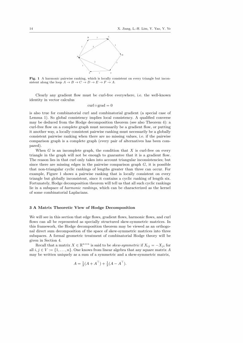
Fig. 1 A harmonic pairwise ranking, which is locally consistent on every triangle but incon-sistent along the loop A→ B → C → D → E → F → A.
Clearly any gradient flow must be curl-free everywhere, i.e. the well-knownidentity in vector calculus
curl ◦ grad = 0
is also true for combinatorial curl and combinatorial gradient (a special case ofLemma 1). So global consistency implies local consistency. A qualified conversemay be deduced from the Hodge decomposition theorem (see also Theorem 4): acurl-free flow on a complete graph must necessarily be a gradient flow, or puttingit another way, a locally consistent pairwise ranking must necessarily be a globallyconsistent pairwise ranking when there are no missing values, i.e. if the pairwisecomparison graph is a complete graph (every pair of alternatives has been com-pared).
When G is an incomplete graph, the condition that X is curl-free on everytriangle in the graph will not be enough to guarantee that it is a gradient flow.The reason lies in that curl only takes into account triangular inconsistencies; butsince there are missing edges in the pairwise comparison graph G, it is possiblethat non-triangular cyclic rankings of lengths greater than three can occur. Forexample, Figure 1 shows a pairwise ranking that is locally consistent on everytriangle but globally inconsistent, since it contains a cyclic ranking of length six.Fortunately, Hodge decomposition theorem will tell us that all such cyclic rankingslie in a subspace of harmonic rankings, which can be characterized as the kernelof some combinatorial Laplacians.
3 A Matrix Theoretic View of Hodge Decomposition
We will see in this section that edge flows, gradient flows, harmonic flows, and curlflows can all be represented as specially structured skew-symmetric matrices. Inthis framework, the Hodge decomposition theorem may be viewed as an orthogo-nal direct sum decomposition of the space of skew-symmetric matrices into threesubspaces. A formal geometric treatment of combinatorial Hodge theory will begiven in Section 4.
Recall that a matrix X ∈ Rn×n is said to be skew-symmetric if Xij = −Xji forall i, j ∈ V := {1, . . . , n}. One knows from linear algebra that any square matrix Amay be written uniquely as a sum of a symmetric and a skew-symmetric matrix,
A = 12 (A+A>) + 1
2 (A−A>).

Ranking with Hodge theory 15
We will denote5
A := {X ∈ Rn×n | X> = −X}, and S := {X ∈ Rn×n | X> = X}.
It is perhaps interesting to note that semidefinite programming takes place in thecone of symmetric positive definite matrices in S but the optimization problemsin this paper take place in the exterior space A.
One simple way to construct a skew-symmetric matrix is to take a vectors = [s1, . . . , sn]> ∈ Rn and define X by
Xij := si − sj .
Note that if X 6= 0, then rank(X) = 2 since it can be expressed as se>− es> withe := [1, . . . , 1]> ∈ Rn. These are in a sense the simplest skew-symmetric matrices— they have the lowest possible rank among non-zero skew-symmetric matrices(recall that the rank of a skew-symmetric matrix is necessarily even). In this paper,we will call these gradient matrices and denote them collectively by MG,
MG := {X ∈ A | Xij = si − sj for some s ∈ Rn}.
For T ⊆(V3
), we define the set of T -consistent matrices as
MT := {X ∈ A | Xij +Xjk +Xki = 0 for all {i, j, k} ∈ T}. (14)
We can immediately observe every X ∈ MG is T -consistent for any T ⊆(V3
), i.e.
MG ⊆MT . Conversely, a matrix X that satisfies
Xij +Xjk +Xki = 0 for every triple {i, j, k} ∈
(V
3
).
is necessarily a gradient matrix, i.e.
MG =M(V3). (15)
Given T ⊆(V3
), it is straightforward to verify that both MG and MT are
subspaces of Rn×n. The preceding discussions then imply
MG ⊆MT ⊆ A. (16)
Since these are strict inclusions in general, several complementary subspaces arisenaturally. With respect to the usual inner product 〈X,Y 〉 = tr(X>Y ) =
∑i,j XijYij ,
we obtain orthogonal complements ofMG andMT in A as well as the orthogonalcomplement of MG in MT , which we denote by MH :
A =MG ⊕M⊥G, A =MT ⊕M⊥T , MT =MG ⊕MH .
Elements of MH will be called harmonic matrices as we will see that they arediscrete analogues of solutions to the Laplace equation (or, more accurately, theHelmholtz equation). An alternative characterization of MH is
MH =MT ∩M⊥G,5 More common notations for A are son(R) (Lie algebra of SO(n)) and ∧2(Rn) (second
exterior product of Rn).
16 X. Jiang, L.-H. Lim, Y. Yao, Y. Ye
which may be viewed as a discrete analogue of the condition of being simul-taneously curl-free and divergence-free. More generally, this discussion appliesto any weighted inner product 〈X,Y 〉w =
∑i,j wijXijYij . The five subspaces
MG,MT ,MH ,M⊥T ,M⊥G of A play a central role in our techniques. As we shallsee later, the Helmholtz decomposition in Theorem 2 may be viewed as the or-thogonal direct sum decomposition
A =MG ⊕MH ⊕M⊥T .
4 Combinatorial Hodge Theory
In this section we will give a brief introduction to combinatorial Hodge theory,paying special attention to its relevance in statistical ranking. One may wonderwhy we do not rely on our relatively simple matrix view in Section 3. The rea-sons are two fold: firstly, important geometric insights are lost when the actualmotivations behind the matrix picture are disregarded; and secondly, the matrixapproach applies only to the case of 2-dimensional simplicial complex but combi-natorial Hodge theory extends to any k-dimensional simplicial complex. While sofar we did not use any simplicial complex of dimension higher than 2 in our studyof statistical ranking, it is conceivable that higher-dimensional simplicial complexcould play a role in future studies.
4.1 Extension of Pairwise Comparison Graph to Simplicial Complex
Let G = (V,E) be a pairwise comparison graph. To characterize the triangularinconsistency or curl, one needs to study the triangles formed by the 3-cliques6,i.e. the set
T (E) :={{i, j, k} ∈
(V3
) ∣∣ {i, j}, {j, k}, {k, i} ∈ E}.A combinatorial object of the form (V,E, T ) where E ⊆
(V2
), T ⊆
(V3
), and
{i, j}, {j, k}, {k, i} ∈ E for all {i, j, k} ∈ T is called a 2-dimensional simplicialcomplex. This is a generalization of a graph, which is a 1-dimensional simplicialcomplex. In particular, given a graph G = (V,E), the 2-dimensional simplicialcomplex (V,E, T (E)) is often called the 3-clique complex of G.
More generally, a simplicial complex (V,Σ) is a vertex set V = {1, . . . , n}together with a collection Σ of subsets of V that is closed under inclusion, i.e. ifτ ∈ Σ and σ ⊂ τ , then σ ∈ Σ. The elements in Σ are called simplices. For example,a 0-simplex is just an element i ∈ V (recall that we do not distinguish between
(V1
)and V ), a 1-simplex is a pair {i, j} ∈
(V2
), a 2-simplex is a triple {i, j, k} ∈
(V3
),
and so on. For k ≤ n, a k-simplex is a (k+1)-element set in(Vk+1
)and Σk ⊂
(Vk+1
)will denote the set of all k-simplices in Σ. In the previous paragraph, Σ0 = V ,Σ1 = E, Σ2 = T , and Σ = V ∪ E ∪ T . In general, given any undirected graphG = (V,E), one obtains a (k − 1)-dimensional simplicial complex Kk
G := (V,Σ)called the k-clique complex7 of G by ‘filling in’ all its j-cliques for j = 1, . . . , k, or
6 Recall that a k-clique of G is just a complete subgraph of G with k vertices.7 Note that a k-clique is a (k − 1)-simplex.
Ranking with Hodge theory 17
more precisely, by setting Σ = {j-cliques of G | j = 1, . . . , k}. When k is maximalKkG is written KG and called the clique complex of G.
In this paper, we will mainly concern ourselves with studying the 3-cliquecomplex K3
G = (V,E, T (E)) where G is a pairwise comparison graph. Note thatwe could also look at the simplicial complex (V,E, Tγ(E)) where
Tγ(E) :={{i, j, k} ∈ T (E)
∣∣ |Xij +Xjk +Xki| ≤ γ}
where 0 ≤ γ ≤ ∞. For γ =∞, we get K3G but for general γ we get a subcomplex of
K3G. We have found this to be a useful multiscale characterization of inconsistencies
but detailed discussion will be left to future work.
4.2 Cochains, Coboundary Maps, and Combinatorial Laplacians
We will now introduce some discrete exterior calculus on a simplicial complexwhere potential functions (scores or utility), edge flow (pairwise ranking), trian-gular flow (triplewise ranking), gradient (global ranking induced by scores), curl(local inconsistency) become just special cases of a much more general framework.We will now also define the notions of combinatorial divergence and combina-torial Laplacians. The 0-dimensional combinatorial Laplacian is the usual graphLaplacian. The case of greatest interest here is the 1-dimensional combinatorialLaplacian, or the graph Helmholtzian.
Definition 4 Let K be a simplicial complex and recall that Σk denotes its setof k-simplices. A k-dimensional cochain is a real-valued function on (k + 1)-tuples of vertices that is alternating on each of the k-simplex and 0 otherwise, i.e.f : V k+1 → R such that
f(iσ(0), . . . , iσ(k)) = sign(σ)f(i0, . . . , ik),
for all (i0, . . . , ik) ∈ V k+1 and all σ ∈ Sk+1, the permutation group on k + 1elements, and that
f(i0, . . . , ik) = 0 if {i0, . . . , ik} /∈ Σk.
The set of all k-cochains on K is denoted Ck(K,R).
For simplicity we often write Ck for Ck(K,R). So C0 is the space of potentialfunctions, C1 the space of edge flows, and C2 the space of triangular flows.
The k-cochain space Ck can be given a choice of inner product. In view of theweighted l2-minimization for our statistical ranking problem (7), we will define thefollowing inner product on C1,
〈X,Y 〉w =∑{i,j}∈E
wijXijYij , (17)
for all edge flows X,Y ∈ C1. In the context of a pairwise comparison graph G,it may not be immediately clear why this defines an inner product since we havenoted after (8) that W = [wij ] is only a nonnegative matrix and it is possiblethat some entries are 0. However observe that by definition wij = 0 iff no votershave rated both alternatives i and j and therefore {i, j} 6∈ E by (4) and so any

18 X. Jiang, L.-H. Lim, Y. Yao, Y. Ye
edge flow X will automatically have Xij = 0 by (5). Hence we indeed have that〈X,X〉w = 0 iff X = 0, as required for an inner product (the other properties aretrivial to check).
The operators grad and curl are special instances of coboundary maps:
Definition 5 The kth coboundary operator δk : Ck(K,R)→ Ck+1(K,R) is thelinear map that takes a k-cochain f ∈ Ck to a (k+ 1)-cochain δkf ∈ Ck+1 definedby
(δkf)(i0, i1, . . . , ik+1) :=∑k+1
j=0(−1)jf(i0, . . . , ij−1, ij+1, . . . , ik+1).
Note that ij is omitted from the jth summand, i.e. coboundary maps computean alternating difference with one input left out. So δ0 = grad, i.e. (δ0s)(i, j) =sj − si, and δ1 = curl, i.e. (δ1X)(i, j, k) = Xij +Xjk +Xki.
Given a choice of an inner product 〈·, ·〉k on Ck, we may define the adjointoperator of the coboundary map, δ∗k : Ck+1 → Ck in the usual manner, i.e.〈δkfk, gk+1〉k+1 = 〈fk, δ∗kgk+1〉k.
Definition 6 The combinatorial divergence operator div : C1(K,R)→ C0(K,R)is the adjoint of δ0 = grad, i.e.
div := −δ∗0 . (18)
Divergence will appear in the minimum norm solution to (7) and can be usedto characterize M⊥G. As usual, we will drop the adjective ‘combinatorial’ whenthere is no cause for confusion.
For statistical ranking, it suffices to consider k = 0, 1, 2. Let G be a pairwisecomparison graph and KG its clique complex8. The cochain maps,
C0(KG,R)δ0−→ C1(KG,R)
δ1−→ C2(KG,R) (19)
and their adjoints,
C0(KG,R)δ∗0←− C1(KG,R)
δ∗1←− C2(KG,R), (20)
have the following ranking theoretic interpretations: C0, C1, C2 represent spacesof score functions, pairwise rankings, triplewise rankings, and
scoresgrad−−−→ pairwise
curl−−→ triplewise,
scores− div=grad∗←−−−−−−−− pairwise
curl∗←−−− triplewise.
Recall that combinatorial gradient, curl, and divergence are defined by
(grad s)(i, j) = (δ0s)(i, j) = sj − si,(curlX)(i, j, k) = (δ1X)(i, j, k) = Xij +Xjk +Xki,
(divX)(i) = −(δ∗0X)(i) =∑
j s.t. {i,j}∈EwijXij
8 It does not matter whether we consider KG or K3G or indeed any Kk
G where k ≥ 3;the higher-dimensional k-simplices where k ≥ 3 do not play a role in the coboundary mapsδ0, δ1, δ2.
Ranking with Hodge theory 19
with respect to the inner product 〈X,Y 〉w =∑{i,j}∈E wijXijYij on C1.
As an aside, it is perhaps worth pointing out that there is no special name forthe adjoint of curl coming from physics because in 3-space, C1 may be identifiedwith C2 via a property called Hodge duality and in which case curl is a self-adjointoperator, i.e. curl∗ = curl. This will not be true in our case.
If we represent functions on vertices by n-vectors, edge flows by n × n skew-symmetric matrices, and triangular flows by n× n× n skew-symmetric hyperma-trices, i.e.
C0 = Rn,
C1 = {[Xij ] ∈ Rn×n | Xij = −Xji} = A,
C2 = {[Φijk] ∈ Rn×n×n | Φijk = Φjki = Φkij = −Φjik = −Φikj = −Φkji},
then in the language of linear algebra introduced in Section 3,
im(δ0) = im(grad) =MG, ker(δ1) = ker(curl) =MT ,
ker(δ∗0) = ker(div) =M⊥G, im(δ∗1) = im(curl∗) =M⊥T ,
where T = T (E).Coboundary maps have the following important property.
Lemma 1 (Closedness) δk+1 ◦ δk = 0.
For k = 0, this and its adjoint are well-known identities in vector calculus,
curl ◦ grad = 0, div ◦ curl∗ = 0. (21)
Ranking theoretically, the first identity simply says that a global ranking must beconsistent.
We will now define combinatorial Laplacians, higher-dimensional analogues ofthe graph Laplacian.
Definition 7 Let K be a simplicial complex. The k-dimensional combinatorialLaplacian is the operator ∆k : Ck(K,R)→ Ck(K,R) defined by
∆k = δ∗k ◦ δk + δk−1 ◦ δ∗k−1. (22)
In particular,
∆0 = δ∗0 ◦ δ0 = −div ◦ grad
is a discrete analogue of the scalar Laplacian or Laplace operator while
∆1 = δ∗1 ◦ δ1 + δ0 ◦ δ∗0 = curl∗ ◦ curl− grad ◦div
is a discrete analogue of the vector Laplacian or Helmholtz operator. In the contextof graph theory, if K = KG, then ∆0 is called the graph Laplacian [12] while ∆1
is called the graph Helmholtzian.The combinatorial Laplacian has some well-known, important properties.
Lemma 2 ∆k is a positive semidefinite operator. Furthermore, the dimension ofker(∆k) is equal to kth Betti number of K.

20 X. Jiang, L.-H. Lim, Y. Yao, Y. Ye
We will call a cochain f ∈ ker(∆k) harmonic since they are solutions to higher-dimensional analogue of the Laplace equation
∆kf = 0.
Strictly speaking, the Laplace equation refers to ∆0f = 0. The equation ∆1X = 0is really the Helmholtz equation. But nonetheless, we will still call an edge flowX ∈ ker(∆1) a harmonic flow.
4.3 Hodge Decomposition Theorem and HodgeRank
We now state the main theorem in combinatorial Hodge theory.
Theorem 1 (Hodge Decomposition Theorem) Ck(K,R) admits an orthog-onal decomposition
Ck(K,R) = im(δk−1)⊕ ker(∆k)⊕ im(δ∗k).
Furthermore,
ker(∆k) = ker(δk) ∩ ker(δ∗k−1).
An elementary proof targeted at a computer science readership may be foundin [19]. For completeness we include a proof here.
Proof We will use Lemma 1. First, Ck = im(δk−1)⊕ ker(δ∗k−1). Since δkδk−1 = 0,taking adjoint yields δ∗k−1δ
∗k = 0, which implies that im(δ∗k) ⊆ ker(δ∗k−1). There-
fore ker(δ∗k−1) = [im(δ∗k)⊕ ker(δk)]∩ ker(δ∗k−1) = [im(δ∗k)∩ ker(δ∗k−1)]⊕ [ker(δk)∩ker(δ∗k−1)] = im(δ∗k) ⊕ [ker(δk) ∩ ker(δ∗k−1)]. It remains to show that ker(δk) ∩ker(δ∗k−1) = ker(∆k) = ker(δk−1δ
∗k−1 + δ∗kδk). Clearly ker(δk) ∩ ker(δ∗k−1) ⊆
ker(∆k). For any X = δ∗kΦ ∈ im(δ∗k) where 0 6= Φ ∈ Ck+1, Lemma 1 againimplies δk−1δ
∗k−1X = δk−1δ
∗k−1δ
∗kΦ = 0, but δ∗kδkX = δ∗kδkδ
∗kΦ 6= 0, which implies
that ∆kX 6= 0. Similarly for X ∈ im(δ0). Hence ker(∆k) = ker(δk)∩ker(δ∗k−1). ut
While Hodge decomposition holds in general for any simplicial complex of anydimension k, the case k = 1 is often called the Helmholtz decomposition theorem9.We will state it here for the special case of a clique complex.
Theorem 2 (Helmholtz Decomposition Theorem) Let G = (V,E) be anundirected, unweighted graph and KG be its clique complex. The space of edgeflows on G, i.e. C1(KG,R), admits an orthogonal decomposition
C1(KG,R) = im(δ0)⊕ ker(∆1)⊕ im(δ∗1)
= im(grad)⊕ ker(∆1)⊕ im(curl∗). (23)
Furthermore,
ker(∆1) = ker(δ1) ∩ ker(δ∗0) = ker(curl) ∩ ker(div). (24)
Ranking with Hodge theory 21
ker(curl)
⊕ ⊕
Inconsistent (divergence-free)
Locally consistent (curl-free)
im(grad)
Harmonic flows
ker(∆1)
Curl flows
im(curl∗)
(locally acyclic)
Gradient flows
(globally acyclic)
ker(div)
(locally cyclic)
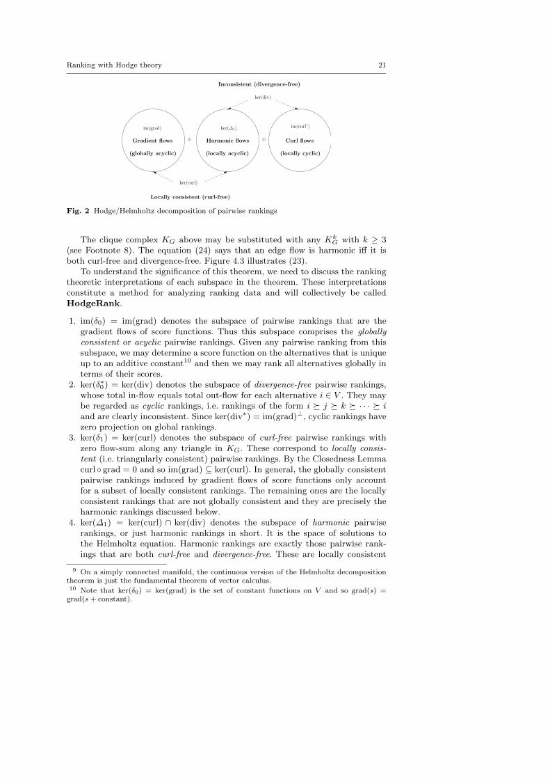
Fig. 2 Hodge/Helmholtz decomposition of pairwise rankings
The clique complex KG above may be substituted with any KkG with k ≥ 3
(see Footnote 8). The equation (24) says that an edge flow is harmonic iff it isboth curl-free and divergence-free. Figure 4.3 illustrates (23).
To understand the significance of this theorem, we need to discuss the rankingtheoretic interpretations of each subspace in the theorem. These interpretationsconstitute a method for analyzing ranking data and will collectively be calledHodgeRank.
1. im(δ0) = im(grad) denotes the subspace of pairwise rankings that are thegradient flows of score functions. Thus this subspace comprises the globallyconsistent or acyclic pairwise rankings. Given any pairwise ranking from thissubspace, we may determine a score function on the alternatives that is uniqueup to an additive constant10 and then we may rank all alternatives globally interms of their scores.
2. ker(δ∗0) = ker(div) denotes the subspace of divergence-free pairwise rankings,whose total in-flow equals total out-flow for each alternative i ∈ V . They maybe regarded as cyclic rankings, i.e. rankings of the form i � j � k � · · · � iand are clearly inconsistent. Since ker(div∗) = im(grad)⊥, cyclic rankings havezero projection on global rankings.
3. ker(δ1) = ker(curl) denotes the subspace of curl-free pairwise rankings withzero flow-sum along any triangle in KG. These correspond to locally consis-tent (i.e. triangularly consistent) pairwise rankings. By the Closedness Lemmacurl ◦ grad = 0 and so im(grad) ⊆ ker(curl). In general, the globally consistentpairwise rankings induced by gradient flows of score functions only accountfor a subset of locally consistent rankings. The remaining ones are the locallyconsistent rankings that are not globally consistent and they are precisely theharmonic rankings discussed below.
4. ker(∆1) = ker(curl) ∩ ker(div) denotes the subspace of harmonic pairwiserankings, or just harmonic rankings in short. It is the space of solutions tothe Helmholtz equation. Harmonic rankings are exactly those pairwise rank-ings that are both curl-free and divergence-free. These are locally consistent
9 On a simply connected manifold, the continuous version of the Helmholtz decompositiontheorem is just the fundamental theorem of vector calculus.10 Note that ker(δ0) = ker(grad) is the set of constant functions on V and so grad(s) =
grad(s+ constant).
22 X. Jiang, L.-H. Lim, Y. Yao, Y. Ye
with zero curl on every triangle in T (E) but not globally consistent. In otherwords, while there are no inconsistencies due to small loops of length 3, i.e.i � j � k � i, there are inconsistencies along larger loops of lengths > 3, i.e.a � b � c � · · · � z � a. So these are also cyclic rankings. Rank aggregationon ker(∆1) depends on edge paths traversed in the simplicial complex; alonghomotopy equivalent paths one obtains consistent rankings. Figure 1 has anexample of harmonic ranking.
5. im(δ∗1) = im(curl∗) denotes the subspace of locally cyclic pairwise rankings thathave non-zero curls along triangles. By the Closedness Lemma, im(curl∗) ⊆ker(div) and so this subspace is in general a proper subspace of the divergence-free rankings; the orthogonal complement of im(curl∗) in ker(div) is preciselythe space of harmonic rankings ker(∆1).
5 Analysis of HodgeRank
We now state two immediate implications of the Helmholtz decomposition theoremwhen applied to statistical ranking. The first implication is that HodgeRank givesan interpretation of the solution and residual of the optimization problem (7); theseare respectively the l2-projection on gradient flows and divergence-free flows. Inthe context of statistical ranking and in the l2-sense, the solution to (7) gives thenearest globally consistent pairwise ranking to the data while the residual givesthe sum total of all inconsistent components (both local and harmonic) in thedata. The second implication is the condition that local consistency guaranteesglobal consistency whenever there is no harmonic component in the data (whichhappens iff the clique complex of the pairwise comparison graph is ‘loop-free’).
5.1 Structure Theorem for Global Ranking and the Residual of Inconsistency
In order to cast our optimization problem (7) in the Hodge theoretic framework,we need to specify a choice of inner products on C0, C1, C2. As before, the innerproduct on the space of edge flows (pairwise rankings) C1 will be a weightedEuclidean inner product:
〈X,Y 〉w =∑{i,j}∈E
wijXijYij
for X,Y ∈ C1. We use unweighted Euclidean inner products on C0 and C2,
〈r, s〉 =∑n
i=1risi, 〈Θ,Φ〉 =
∑{i,j,k}∈T (E)
ΘijkΦijk
for r, s ∈ C0 and Θ,Φ ∈ C2. This is mainly to keep our notations uncluttered.Other choices could be made (e.g. inner products on C0 and C2 could have beenweighted) with corresponding straightforward modification of (7) but this wouldnot change the essential nature of our methods.
The optimization problem (7) is then equivalent to an l2-projection of an edgeflow representing a pairwise ranking onto im(grad),
mins∈C0
‖δ0s− Y ‖2,w = mins∈C0
‖ grad s− Y ‖2,w.
Ranking with Hodge theory 23
The Helmholtz decomposition theorem then leads to the following result aboutthe structure of solutions and residuals of (7). In Theorem 3 below, we assumethat the pairwise ranking data Y has been estimated from one of the methodsin Section 2.3. The least squares solution s will be a score function that inducesgrad s, the l2-nearest global ranking to Y . Since s is only unique up to a constant(see Footnote 10), we determine a unique minimum norm solution s∗ for the sakeof well-posedness; but nevertheless any s will yield the same global ordering ofalternatives. The least squares residual R∗ represents the inconsistent componentof the ranking data Y . The magnitude of R∗ is a ‘certificate of reliability’ for s;since if this is small, then the globally consistent component grad s accounts formost of the variation in Y and we may conclude that s gives a reasonably reliableranking of the alternatives. But even when the magnitude of R∗ is large, we will seethat it may be further resolved into a global and a local component that determinewhen a comparison of alternatives with respect to s is valid.
Theorem 3 (i) Solutions of (7) satisfy the following normal equation
∆0s = −div Y , (25)
and thus the minimum norm solution is
s∗ = −∆†0 div Y (26)
where † indicates Moore-Penrose inverse. The divergence in (26) is
(div Y )(i) =∑
j s.t. {i,j}∈Ewij Yij ,
and the matrix representing the graph Laplacian is given by
[∆0]ij =
∑i wii if j = i,
−wij if j is such that {i, j} ∈ E,0 otherwise.
(ii) The residual R∗ = Y − δ0s∗ is divergence-free, i.e. divR∗ = 0. Moreover, ithas a further orthogonal decomposition
R∗ = projim(curl∗) Y + projker(∆1) Y , (27)
where projim(curl∗) Y is a locally cyclic ranking accounting for local inconsis-
tencies and projker(∆1) Y is a harmonic ranking accounting for global incon-sistencies. In particular, the projections are given by
projim(curl∗) = curl† curl and projker(∆1) = I −∆+1 ∆1. (28)
Proof The normal equation for mins∈C0 ‖δ0s− Y ‖22,w is
δ∗0δ0s = δ∗0 Y .
(25), (26), and divR∗ = 0 are obvious upon substituting ∆0 = δ∗0δ0 and div =−δ∗0 . The expressions for divergence and graph Laplacian in (i) follow from theirrespective definitions. The Helmholtz decomposition theorem implies
ker(∆1)⊕ im(curl∗) = im(grad)⊥.

24 X. Jiang, L.-H. Lim, Y. Yao, Y. Ye
Obviously projim(grad)⊥ grad s∗ = 0. Since R∗ = Y − grad s∗ is a least squares
residual, we must have projim(grad)R∗ = projim(grad) Y − grad s∗ = 0. These
observations yield (27), as
R∗ = projim(grad)R∗ + projim(grad)⊥ R
∗ = 0 + projker(∆1)⊕im(curl∗) Y .
The expressions for the projections in (28) are standard. ut
In the special case when the pairwise ranking matrix G is a complete graphand we have an unweighted Euclidean inner product on C1, the minimum normsolution s∗ in (26) satisfies
∑i s∗i = 0 and is given by
s∗i = − 1
ndiv(Y )(i) = − 1
n
∑jYij . (29)
In Section 6, we shall see that this is the well-known Borda count in social choicetheory, a measure that is also widely used in psychology and statistics [28,33,14].Since G is a complete graph only when the ranking data is complete, i.e. everyvoter has rated every alternative, this is an unrealistic scenario for the type ofmodern ranking data discussed in Section 1. Among other things, HodgeRankgeneralizes Borda count to scenarios where the ranking data is incomplete or evenhighly incomplete.
In (ii) the locally cyclic ranking component is obtained by solving
minΦ∈C2
‖ curl∗ Φ−R∗‖2,w = minΦ∈C2
‖ curl∗ Φ− Y ‖2,w.
The above equality implies that there is no need to first solve for R∗ before wemay obtain Φ; one could get it directly from the pairwise ranking data Y . Notethat the solution is only determined up to an additive term of the form grad ssince by virtue of (21),
curl(Φ+ grad s) = curlΦ. (30)
For the sake of well-posedness, we seek the unique minimum norm solution
Φ∗ = (δ1 ◦ δ∗1)†δ1Y = (curl ◦ curl∗)† curl Y
and the required component is given by projim(curl∗) Y = curl∗ Φ∗. The reader mayhave noted a parallel between the two problems
mins∈C0‖grad s− Y ‖2,w and min
Φ∈C2‖curl∗ Φ− Y ‖2,w.
Indeed in many contexts, s is called the scalar potential while Φ is called the vectorpotential. As seen earlier in Definition 1, an edge flow of the form grad s for somes ∈ C0 is called a gradient flow; in analogy, we will call an edge flow of the formcurl∗ Φ for some Φ ∈ C2 a curl flow.
We note that the l2-residual R∗, being divergence-free, is a cyclic ranking.Much like (30), the divergence-free condition is satisfied by a whole family of edgeflows that differ from R∗ only by a term of the form curl∗ Φ since
div(R∗ + curl∗ Φ) = divR∗
because of (21). The subset of C1 given by
{R∗ + curl∗ Φ | Φ ∈ C2}

Ranking with Hodge theory 25
is called the homology class of R∗. The harmonic ranking projker(∆1) Y is just one
element in this class11. In general, it will be dense in the sense that it will benonzero on almost every edge in E. This is because in addition to the divergence-free condition, the harmonic ranking must also satisfy the curl-free condition byvirtue of (24). So if parsimony or sparsity is the objective, e.g. if one wants to iden-tify a small number of conflicting comparisons that give rise to the inconsistenciesin the ranking data, then the harmonic ranking does not offer much informationin this regard. To better understand ranking inconsistencies via the structure ofR∗, it is often helpful to look for elements in the same homology class with thesparsest support, i.e.
minΦ∈C2
‖curl∗ Φ−R∗‖0 = minΦ∈C2
‖curl∗ Φ− projker(∆1) Y ‖0.
The widely used convex relaxation replacing the l0-‘norm’ by the l1-norm maybe employed [23], i.e.
minΦ∈C2
‖curl∗ Φ−R∗‖1 := minΦ∈C2
∑i,j|(curl∗ Φ)ij −R∗ij |.
A solution Φ of such an l1-minimization problem is expected to give a sparse el-ement R∗ − curl∗ Φ. The bottom line here is that we want to find the shortestcycles that represent the global inconsistencies and perhaps remove the corre-sponding edges in the pairwise comparison graph, in view of what we will discussnext in Section 5.2. One plausible strategy to get a globally consistent ranking is toremove a number of problematic ‘conflicting’ comparisons from the pairwise com-parison graph. Since it is only reasonable to remove as few edges as possible, thistranslates to finding a homology class with the sparsest support. This is similarto the minimum feedback arc set approach discussed in Section 6.2.
We will end the discussion of this section with a note on computational costsof HodgeRank. Solving for a global ranking s∗ in (26) only requires the solutionof an n×n least squares problem, which comes with a modest cost of O(n3) flops(n = |V |). As we note later in Section 7.3, for web ranking analysis such a costis no more than computing the PageRank. On the other hand, the analysis ofinconsistency is generally harder. For example, evaluating curls requires |T | flopsand this is
(n3
)∼ O(n3) in the worst case. Since an actual computation of Φ∗
involves solving a least squares problem of size |T | × |T |, the computation costincurred is of order O(n9). Nevertheless, any sparsity in the data (when |T | � n3)may be exploited by choosing the right least squares solver. For example, one mayuse the general sparse least squares solver lsqr [35] or the new minres-qlp [9,10]that works specifically for symmetric matrices. We will leave discussions of actualcomputations and more extensive numerical experiments to a future article. Itsuffices to note here that it is in general harder to isolate the harmonic componentof ranking data than the globally consistent component.
5.2 Local Consistency versus Global Consistency
In this section, we discuss a useful result, that local consistency implies globalconsistency whenever the harmonic component is absent from the ranking data.
11 Two elements of the same homology class are called homologous.

26 X. Jiang, L.-H. Lim, Y. Yao, Y. Ye
Whether a harmonic component exists is dependent on the topology of the cliquecomplex K3
G. We will invoke the recent work of Kahle [24] on topological propertiesof random graphs to argue that harmonic components are exceedingly unlikely tooccur.
By Lemma 2, the dimension of ker(∆1) is equal to the first Betti numberβ1(K) of the underlying simplicial complex K. Since ker(∆1) = 0 if β1(K) = 0,the harmonic component of any edge flow on K is automatically absent whenβ1(K) = 0 (roughly speaking, β1(K) = 0 means that K does not have any 1-dimensional holes). This leads to the following result.
Theorem 4 Let K3G = (V,E, T (E)) be a 3-clique complex of a pairwise compari-
son graph G = (V,E). If K3G does not contain any 1-loops, i.e. β1(K3
G) = 0, thenevery locally consistent pairwise ranking is also globally consistent. In other words,if the edge flow X ∈ C1(K3
G,R) is curl-free, i.e.
curl(X)(i, j, k) = 0
for all {i, j, k} ∈ T (E), then it is a gradient flow, i.e. there exists s ∈ C0(KG,R)such that
X = grad s.
Proof This follows from Helmholtz decomposition since dim(ker∆1) = β1(K3G) =
0 and so any X that is curl-free is automatically in im(grad). ut
When G is a complete graph, then we always have β1(KG) = β1(K3G) = 0
and this justifies the discussion after Definition 3 about the equivalence of localand global consistencies for complete pairwise comparison graphs. In general, Gwill be incomplete due to missing data (not all voters have rated all alternatives)but as long as K3
G is loop-free, such a claim still holds. In finance, this theo-rem translates into the well-known result that “triangular arbitrage-free impliesarbitrage-free.” The theorem enables us to infer global consistency from a localcondition — whether the ranking data is curl-free. We note that being curl-freeis a strong condition. If we instead have “triangular transitivity” in the ordinalsense, i.e. a � b � c implies a � c, then there is no result analogous to Theorem 4.
At least for Erdos-Renyi random graphs, the Betti number β1 could only benon-zero when the edges are neither too sparse nor too dense. The following resultby Kahle [24] quantifies this statement. He showed that β1 undergoes two phasetransitions from zero to nonzero and back to zero as the density of edges grows.
Theorem 5 (Kahle 2006) For an Erdos-Renyi random graph G(n, p) on n ver-tices where the edges are independently generated with probability p, its clique com-plex KG almost always has β1(KG) = 0, except when
1
n2� p� 1
n. (31)
Without getting into a discussion as to whether an Erdos-Renyi random graphis a good model for pairwise comparison graphs of real-world ranking data, wenote that the Netflix pairwise comparison graph has a high probability of havingβ1(KG) = 0 if Kahle’s result applies. Although the original customer-productrating matrix of the Netflix prize dataset is highly incomplete (more than 99%missing values), its pairwise comparison graph is very dense (less than 0.22%missing edges). So p (probability of an edge) and n (number of vertices) are bothlarge and (31) is not satisfied.

Ranking with Hodge theory 27
6 Connections to Social Choice Theory
Social choice theory is almost undoubtedly the discipline most closely associatedwith the study of ranking, having a long history dating back to Condorcet’s famoustreatise in 1785 [11] and a large body of work that led to at least two Nobel prizes[3,39].
The famous impossibility theorems of Arrow [2] and Sen [38] in social choicetheory formalized the inherent difficulty of achieving a global ranking of alterna-tives by aggregating over the voters. However it is still possible to perform anapproximate rank aggregation in reasonable, systematic ways. Among the variousproposed methods, the best known ones are those by Condorcet [11], Borda [15],and Kemeny [25]. The Kemeny approach is often regarded as the best approximaterank aggregation method under some assumptions [43,42]. It is however NP-hardto compute and its sole reliance on ordinal information may be unnatural forscore-based cardinal data.
We have described earlier how the minimization of (7) over the gradient flowmodel class
MG = {X ∈ C1 | Xij = sj − si, s : V → R}
leads to a Hodge theoretic generalization of Borda count but the minimization of(7) over the Kemeny model class
MK = {X ∈ C1 | Xij = sign(sj − si), s : V → R}
leads to Kemeny optimization. We will elaborate on these in Section 6.1.
The following are some desirable properties of ranking data that have beenwidely studied, used, and assumed in social choice theory. A ranking problem iscalled complete if each voter in Λ gives a total ordering or permutation of allalternatives in V ; this implies that wαij > 0 for all α ∈ Λ and all distinct i, j ∈ V ,in the terminology of Section 2. It is balanced if the pairwise comparison graphG = (V,E) is k-regular with equal weights wij = c for all {i, j} ∈ E. A completeand balanced ranking induces a complete graph with equal weights on all edges.Moreover, it is binary if every pairwise comparison is allowed only two values,say, ±1 without loss of generality. So Y αij = 1 if voter α prefers alternative j toalternative i, and Y αij = −1 otherwise. Ties are disallowed to keep the discussionsimple.
Classical social choice theory often assumes complete, balanced, and binaryrankings. However, these are all unrealistic assumptions for modern data comingfrom internet and e-commerce applications. Take the Netflix dataset for illustra-tion, a typical user α of Netflix would have rated at most a very small fractionof the entire Netflix inventory. Indeed, as we have mentioned in Section 2.2.1, theviewer-movie rating matrix has 99% missing values. Moreover, while blockbustermovies would receive a disproportionately large number of ratings, since just aboutevery viewer has watched them, the more obscure or special interest movies wouldreceive very few ratings. In other words, the Netflix dataset is highly incompleteand highly imbalanced. Furthermore, the Netflix ratings are given in terms ofscores, i.e. 1 through 5 stars. While it is possible to ignore the cardinal natureof the dataset and just use its ordinal information to construct a binary pairwiseranking, we would be losing valuable information — for example, a 5-star versus

28 X. Jiang, L.-H. Lim, Y. Yao, Y. Ye
1-star comparison is indistinguishable from a 3-star versus 2-star comparison whenone only takes ordinal information into account.
Therefore, one is ill-advised to apply methods from classical social choice the-ory to modern ranking data directly. We will see next that our Hodge theoreticextension of Borda count adapts to these new features in modern datasets, i.e.incomplete, imbalanced, cardinal data, but restricts to the usual Borda count fordata that is complete, balanced, and ordinal/binary.
6.1 Kemeny Optimization and Borda Count
The basic idea of Kemeny’s rule [25,26] is to minimize the number of pairwisemismatches from a given ordering of alternatives to a voting profile, i.e. the col-lection of total orders on the alternatives by each voter. The minimizers are calledKemeny optima and are often regarded as the most reasonable candidates for aglobal ranking of the alternatives. To be precise, we define the binary pairwiseranking associated with a permutation σ ∈ Sn (the permutation group on n ele-ments) to be Y σij = sign(σ(i) − σ(j)). Given two total orders or permutations onthe n alternatives, σ, τ ∈ Sn, the Kemeny distance (also known as Kemeny-Snellor Kendall τ distance) is defined as
dK(σ, τ) :=1
2
∑i<j|Y σij − Y τij | =
1
4
∑i,j|Y σij − Y τij |,
i.e. the number of pairwise mismatches between σ and τ . Given a voting profileas a set of permutations on V = {1, . . . , n} by m voters, {τi ∈ Sn | i = 1, . . . ,m},the following combinatorial minimization problem
minσ∈Sn
∑m
i=1dK(σ, τi) (32)
is called Kemeny optimization and is known to be NP-hard [17] with respect to nwhen m ≥ 4. For binary-valued rankings with Y αij ∈ {±1},
minX∈MK
∑α,i,j
wαij(Xij − Y αij )2, (33)
counts up to a constant the number of pairwise mismatches from a total order.Hence for a complete, balanced, and binary-valued ranking problem, our mini-mization problem (7) becomes Kemeny optimization if we replace the subspaceMG by the discrete subset MK .
Another well-known method for rank aggregation is the Borda count [15], whichassigns a voter’s top ith alternative a position-based score of n − i; the globalranking on V is then derived from the sum of its scores over all voters. This isequivalent to saying that the global ranking of the ith alternative is derived fromthe score
sB(i) = −∑m,n
α,k=1Y αik, (34)
i.e. the alternative that has the most pairwise comparisons in favor of it from allvoters will be ranked first, and so on. As we have found in (29), the minimumnorm solution of the l2-projection onto gradient flows is given by
s∗(i) = − 1
n
∑kYik = −c
∑m,n
α,k=1Y αik,
Ranking with Hodge theory 29
where c is a positive constant. Hence for a complete, balanced, and binary rank-ing problem, HodgeRank yields the Borda count (up to a positive multiplicativeconstant that has no effect on the ordering of alternatives by scores).
6.2 Comparative Studies
The following theorem gives three equivalent characterizations of (33) when Y αij ∈{±1}. Note that we do not assume complete nor balanced data.
Theorem 6 Suppose that Y αij ∈ {±1}. The following optimization problems areall equivalent:
(i) The weighted least squares problem,
minX∈MK
∑α,i,j
wαij(Xij − Y αij )2,
where MK = {X ∈ A | Xij = sign(sj − si), s : V → R}.(ii) The linear programming problem,
maxX∈K1
〈X, Y 〉 = maxX∈K1
∑{i,j}∈E
wijXij Yij , (35)
where K1 is the set{∑σ∈SnµσP
σ∣∣∣ ∑σµσ = 1, µσ ≥ 0, Pσij = sign(σ(j)− σ(i))
}.
(iii) The weighted l1-minimization problem,
minX∈K2
‖X − Y ‖1,w = minX∈K2
∑{i,j}∈E
wij |Xij − Yij |, (36)
where K2 is the set
{X ∈ A | (sj − si)Xij ≥ 0 for some s : V → R and {i, j} ∈ E}.
(iv) The minimum feedback arc set of the weighted directed graph GW◦Y = (V,E,W◦Y ), whose vertex set is V , directed edge (i, j) ∈ E ⊆ V × V iff Yij > 0 withweight wij Yij.
Proof Assuming (i). Since Xij ∈ {±1}, the problem in (i) is equivalent to
maxX∈MK
∑{i,j}∈E
wijXij Yij . (37)
Since MK is a discrete set containing n! points, a linear programming problemover MK is equivalent to searching over its convex hull, i.e. K1, which gives (ii).
(iv) can also be derived from (37). Consider a weighted directed graph GW◦Ywhere an edge (i, j) ∈ E iff Yij > 0, and in which case has weight |wij Yij |. (37) isequivalent to finding a directed acyclic graph by reverting a set of edge directionswhose weight sum is minimized. This is exactly the minimum feedback arc setproblem.
Finally, we show that (iii) is also equivalent to the minimum feedback arc setproblem. For any X ∈ K2, the transitive region, there is an associated weighted

30 X. Jiang, L.-H. Lim, Y. Yao, Y. Ye
directed acyclic graph GW◦X where an edge (i, j) ∈ E iff Xij > 0, and in whichcase has weight |wijXij |. Note that a minimizer of (36) has either X∗ij = −X∗ji =Yij or X∗ij = −X∗ji = 0 on an edge {i, j} ∈ E, which is equivalent to the problemof finding a directed acyclic graph by deleting a set of edges from GW◦Y suchthat the sum of their weights is minimized. Again, this is exactly the minimumfeedback arc set problem. ut
The set K1 is the convex hull of skew-symmetric permutation matrices Pσ asdefined in [43]. The set K2 is called the transitive pairwise region in [36], comprisingn! cones corresponding to each of the n! permutations on V .
It is known that the minimum feedback arc set problem in (iv) is NP-hard, andtherefore, so are the other three. Moreover, (iii) provides some geometric insightswhen viewed alongside (7), the l2-projection onto gradient flows MG = {X ∈ A |Xij = sj − si, s : V → R}, which we have seen to be a Hodge theoretic extensionof Borda count. We will illustrate their differences and similarities pictorially viaan example from [36].
Consider the simplest case of three-item comparison with V = {i, j, k}. Forsimplicity, we will assume that wij = wjk = wki = 1 and Yij , Yjk, Yki ∈ [−1, 1].Figure 3 shows the unit cube in R3. We will label the coordinates in R3 as[Xij , Xjk, Xki] (instead of the usual [x, y, z]). The shaded plane corresponds tothe set where Xij + Xjk + Xki = 0 in the unit cube. Note that this set isequal to the model class MG because of (15). On the other hand, the transi-tive pairwise region K2 consists of the six orthants within the cube with vertices{±1,±, 1,±1} − {[1, 1, 1], [−1,−1,−1]}. The HodgeRank optimization (7) is thel2-projection onto the plane Xij+Xjk+Xki = 0, while by (iii), Kemeny optimiza-tion (33) is the l1-projection onto the aforementioned six orthants representing thetransitive pairwise region K2. The shaded plane in Figure 3 is a special case of apermutahedron or permutohedron. We refer the reader to [32,44] for excellent dis-cussions of these. In particular, Zhang has shown [44] that the projection depictedin Figure 3 for three-item comparison can be generalized to a comparison of anarbitrary number of items.
In the setting of social choice theory, the following theorem [36] connects orderrelations between Kemeny optimization and Borda count.
Theorem 7 (Saari-Merlin 2000) The Kemeny winner (most preferred) is al-ways strictly above the Kemeny loser (least preferred) under the Borda count; sim-ilarly the Borda winner is always strictly above the Borda loser under the Kemenyrule. Aside from these constraints, the two methods may generate arbitrarily dif-ferent total orders.
The Kemeny rule has several desirable properties in social choice theory whichthe Borda count lacks [43]. The Kemeny rule satisfies the Condorcet rule, in thesense that if an alternative in V wins all pairwise comparisons against other al-ternatives in V , then it must be the overall winner. A Condorcet winner is anyalternative i such that
∑j sign(
∑α Y
αij ) = n. Note that the Condorcet winner
may not exist in general but Kemeny or Borda winners always exist. However, if aCondorcet winner exists, then it must be the Kemeny winner. On the other hand,Borda count can only ensure that the Condorcet winner is ranked strictly abovethe Condorcet loser (least preferred). Another major advantage of the Kemenyrule is its consistency in global rankings under the elimination of alternatives in

Ranking with Hodge theory 31
������������������������������������������������������������������������������������������������������������������������������������������������������������������������������������������������������������������������������������������������������������������������������������������������������������������������������������������������������������������������������������������������������������������������������������������������������������������������������������������������������������������������������������������������������������������������������������������������������������������������������������������������������������������������������������������������������������������������������������������������������������������������������������������������������������������������������������������������������������������������������������������������
������������������������������������������������������������������������������������������������������������������������������������������������������������������������������������������������������������������������������������������������������������������������������������������������������������������������������������������������������������������������������������������������������������������������������������������������������������������������������������������������������������������������������������������������������������������������������������������������������������������������������������������������������������������������������������������������������������������������������������������������������������������������������������������������������������������������������������������������������������������������������������������������
X(k,i)
X(j,k)
(−1,−1,1) (−1,1,1)
(−1,1,−1)
(1,1,1)
O
X(i,j) (−1,−1,−1)
(1,−1,1)
(1,−1,−1) (1,1,−1)
Fig. 3 The shaded region is the subspace Xij +Xjk +Xki = 0. The transitive region consistsof six orthants whose corresponding vertices belong to {±1,±, 1,±1}−{[1, 1, 1], [−1,−1,−1]}.The Borda count is the l2-projection onto the shaded plane while the Kemeny optimization isthe l1-projection onto the transitive region.
V . The Borda count and many other position-based rules fail to meet this condi-tion. In fact, the Kemeny rule is the unique rule [43] that meets all of following: (1)satisfies the Condorcet rule, (2) consistency under elimination, and (3) a naturalproperty called neutral (which we will not discuss here).
Despite the many important features that the Kemeny rule has, its high com-putational cost (NP-hard) makes simpler rules like Borda count attractive in prac-tice, especially when there is large number of alternatives to be ranked. Moreover,in cardinal rankings where it is desirable to preserve the magnitude of score dif-ferences [13] and not just the order relation, using the Hodge theoretic variant ofBorda count with model classMG becomes more relevant than Kemeny optimiza-tion with model class MK .
7 Experimental Studies
We present three examples of analysis of real data using HodgeRank with the hopethat they would illustrate the basic ideas.
The first example ranks movies from the Netflix dataset. We show that (i)HodgeRank reduces temporal drift bias, and (ii) the triangular curls provide ametric for characterizing inconsistencies in the ranking data. The second exam-ple illustrates the use of HodgeRank for finding a universal equivalent or pricefunction (i.e. global ranking) in a currency exchange market, with data from Ya-hoo! Finance. The third example describes how the global ranking component inHodgeRank may be used to approximate PageRank via reversible Markov chains,with data from Webometrics.
7.1 Movie Ranking on a Subset of Netflix Data
The Netflix prize dataset12 contains about 17, 000 movies rated by 480, 000 cus-tomers over 74 months from November 1999 to December 2005. Each customerrated 209 movies on average and around 99% of the ratings are absent from the
12 Available from http://www.netflixprize.com.

32 X. Jiang, L.-H. Lim, Y. Yao, Y. Ye
20 40 602
2.5
3
3.5
4
4.5
5Shakespeare in Love
Ave
rage
Sco
re
20 40 602
2.5
3
3.5
4
4.5
5Witness
20 40 602
2.5
3
3.5
4
4.5
5October Sky
20 40 602
2.5
3
3.5
4
4.5
5The Waterboy
Ave
rage
Sco
re
20 40 602
2.5
3
3.5
4
4.5
5Interview with the Vampire
Month Number20 40 60
2
2.5
3
3.5
4
4.5
5Dune
Fig. 4 Average scores of 6 selected movies over 74 months. The three movies in the top rowhas a decreasing trend in monthly average scores, while in a contrast the other three moviesin the bottom row exhibits an increasing trend.
customer-product matrix. We do not seek to address the Netflix prize problem ofratings prediction here. Instead we take advantage of this rare publicly availabledataset and use it to test the rank aggregation capabilities of our method. Wewould like to aggregate viewers’ ratings into a global ranking on movies, and tomeasure the reliability of such a global ranking. Note that such rank aggregationcould be personalized if one also attempts to identify groups of viewers sharingsimilar tastes (say, via the suggestion in Footnote 2). This could then be used forrating prediction if desired.
For reasons that we will soon explain, we restrict our selections to movies thatreceived ratings on all of the 74 months. There are not many such movies — only25 in all. Several of these have monthly average scores that show substantial up-ward or downward drifts. In Figure 4, we show the temporal variations in scoresof six of these (numerical indices in the Netflix dataset are given in parenthe-ses): Dune (17064), Interview with the Vampire (8079), October Sky (12473),Shakespeare in Love (17764), The Waterboy (14660), and Witness (15057). Suchtemporal variations make it dubious to rank movies by simply taking average scoreover all users, as ratings over different time periods may not be comparable un-der the same scale. It is perhaps worth noting that understanding the temporaldynamics in the Netflix dataset has been a key factor in the approach of Belland Koren [6]. We will see below that the use of HodgeRank provides an effectivemethod to globally rank these movies, detect any inherent inconsistency, and isrobust under temporal variations.

Ranking with Hodge theory 33
Formation of pairwise ranking. Since pairwise rankings are relative measures,we expect them to reduce the effect of temporal drift. Using only ratings bythe same customer in the same month, we employ three of the statistics de-scribed in Section 2.3 to form our pairwise rankings, i.e. the arithmetic meanof score differences (9), the geometric mean of score ratios (10), and the binarycomparisons (11). Since there is nothing to suggest that a logarithmic scale isrelevant, the logarithmic odds ratio gives rather poor result as expected andwe omitted it. For comparison, we compute the mean score of each movie overall customers, ignoring temporal information. A reference score is collected in-dependently from MRQE (Movie Review Query Engine)13, the largest onlinedirectory of movie reviews on the internet.
Global ranking with HodgeRank. We then solve the regression problem in(7) to obtain a projection of pairwise ranking flows onto gradient flows, asgiven by Theorem 3(i). Note that in this example, the pairwise ranking graph iscomplete with n = 6 nodes. Table 1 collects the comparisons between differentglobal rankings. The reference order of movies is again via the MRQE scores.
Inconsistencies and curls. Since the pairwise ranking graph is complete, itsclique complex is a simplex with n = 6 vertices and so the harmonic term inthe HodgeRank is always zero. Hence the residual in Theorem 3 is just the curlprojection, i.e. R∗ = projim(curl∗) Y . We will define two indices of inconsistencyto evaluate the results. The first, called cyclicity ratio, is a measure of globalinconsistency given by Cp = ‖R∗‖22,w/‖Y ‖22,w; while the second, called relativecurl, quantifies the local inconsistency, and is given by the following functionof edges and triangles,
cr({i, j}, {i, j, k}) =(curl Y )(i, j, k)
3(grad s∗)(i, j)=Yij + Yjk + Yki
3(s∗j − s∗i ).
Note that on every triangle {i, j, k} the curl Yij + Yjk + Yki measures thetotal sum of cyclic flow, therefore cr measures the magnitude of its inducededge flow relative to the gradient edge flow of the global ranking s∗. If cr hasabsolute value larger than 1, then the average cyclic flow has an effect largerthan the global ranking s∗, which indicates that the global ranking s∗ mightbe inconsistent on the pair of items.
Table 1 shows that in terms of cyclicity ratio, the best global ranking is obtainedfrom HodgeRank with binary comparisons, which has the smallest cyclicity ratio,0.30. This global ranking is quite different from merely taking mean scores and isa better predictor of MRQE.
A closer look at relative curls allows us to identify the dubious scores. Wewill see that the placement of Witness and October Sky according to the globalranking contains significant inconsistency and should not be trusted. This incon-sistency is largely due to the curls in the triangles t1 = {Witness, October Sky,The Waterboy}, t2 = {Witness, October Sky, Interview with the Vampire}. Infact, there are only two relative curls whose magnitudes exceed 1; both occurredon triangles that contain the edge e = {Witness, October Sky}. The relative curlof t1 with respect to e is 3.6039 while that of t2 with respect to e is 4.1338. As wecan see from Table 1, the inconsistency (large curl) manifests itself as instability
13 Available from http://www.mrqe.com.

34 X. Jiang, L.-H. Lim, Y. Yao, Y. Ye
Global ranking (Score)
Movie MRQE Mean Hodge-Difference Hodge-Ratio Hodge-Binary
Shakespeare in Love 1 (85) 2 (3.87) 1 (0.247) 2 (0.0781) 1 (0.138)Witness 2 (77) 3 (3.86) 2 (0.217) 1 (0.0883) 3 (0.107)
October Sky 3 (76) 1 (3.93) 3 (0.213) 3 (0.0775) 2 (0.111)The Waterboy 4 (66) 6 (3.38) 6 (−0.464) 6 (−0.1624) 6 (−0.252)
Interview with the Vampire 5 (65) 4 (3.71) 4 (−0.031) 4 (−0.0121) 4 (−.012)Dune 6 (44) 5 (3.49) 5 (−0.183) 5 (−0.0693) 5 (−0.092)
Cyclicity ratio – – 0.77 1.15 0.30
Table 1 Global ranking of selected six movies via different methods: MRQE, mean scoreover customers, HodgeRank with arithmetic mean score difference, HodgeRank with geometricmean score ratio, and HodgeRank with binary comparisons. It can be seen that the HodgeRankwith binary comparisons has the smallest inconsistency in terms of the cyclicity ratio.
in the placement of Witness and October Sky — the results vary across differentrank aggregation methods with no possibility of consensus. This illustrates the useof curl as a certificate of validity for global ranking.
7.2 Currency Exchange Market
This example illustrates a globally consistent pairwise ranking on a complete graphusing currency exchange data taken from Yahoo! Finance14. Consider a currencyexchange market with V representing a collection of seven currencies, USD, JPY,EUR, CAD, GBP, AUD, and CHF. Here G = (V,E) is a complete graph sinceevery two currencies in V are exchangeable. Table 2 shows the exchange rates.By logarithmic transform the exchange rates is converted into pairwise rankingsas in Example 2.2.2. The global ranking given by (26) (where δ∗0 = δ>0 ) defines auniversal equivalent that measures the ‘value’ of each currency. As the reader cancheck, the logarithmic transform of the data in Table 2 is curl-free (up to machineprecision), which in this context means triangular arbitrage-free. In other words,there is no way one could profit from a cyclic exchange of any three currencies inV . Since G is a complete graph, the data has no harmonic components; so Hodgedecomposition tells us that local consistency must imply global consistency, whichin this context means arbitrage-free, i.e. there is no way one could profit from acyclic exchange of any number of currencies in V either.
7.3 Comparisons with PageRank and HITS
We apply HodgeRank to the problem of web ranking, which we assumed hereto mean any static linked objects, not necessarily the World Wide Web. As weshall see, HodgeRank provides an alternative to PageRank [8] and HITS [29]. Inparticular, it gives a new way to approximate PageRank and enables us to studythe inconsistency or cyclicity in PageRank models.
Consider a link matrix L where Lij is the number of links from site i to j. Thereare two well-known spectral approach to computing the global rankings of websites
14 Available from http://finance.yahoo.com/currency-converter.

Ranking with Hodge theory 35
Currency exchange rate table
USD JPY EUR CAD GBP AUD CHF
1 USD = 1.0000 114.6700 0.6869 0.9187 0.4790 1.0768 1.14391 JPY = 0.0087 1.0000 0.0060 0.0080 0.0042 0.0094 0.01001 EUR = 1.4558 166.9365 1.0000 1.3374 0.6974 1.5676 1.66531 CAD = 1.0885 124.8177 0.7477 1.0000 0.5214 1.1721 1.24511 GBP = 2.0875 239.3791 1.4340 1.9178 1.0000 2.2478 2.38791 AUD = 0.9287 106.4940 0.6379 0.8532 0.4449 1.0000 1.06231 CHF = 0.8742 100.2448 0.6005 0.8031 0.4188 0.9413 1.0000
Univ. equiv. 1.7097 0.0149 2.4890 1.8610 3.5691 1.5878 1.4946
Table 2 The last line is given by exp(−x∗) where x∗ is the solution to (26). The data wastaken from the Currency Converter Yahoo! Finance on November 6, 2007.
from L, HITS and PageRank. HITS computes the singular value decompositionL = UΣV >, where the primary left-singular vector u1 gives the hub ranking andthe primary right-singular vector v1 gives the authority ranking (both u1 and v1 arenonnegative real-valued by the Perron-Frobenius theorem). PageRank constructs
from L a Markov chain on the sites given by Pij =αLij∑j Lij
+ 1−αn , where n is
the number of sites and α = 0.85 trades-off between Markovian link jumps andrandom surfing.
It is clear that we may define an edge flow via
Yij = logPijPij
. (38)
However what property does such a flow capture in PageRank? To answer thisquestion we will need to recall the notion of a reversible Markov chain: An irre-ducible Markov chain with transition matrix P and stationary distribution π isreversible if πiPij = πjPji. Therefore a reversible Markov chain P has a pairwiseranking flow induced from a global ranking, Yij = log(Pij/Pij) = log πj − log πi,where log π gives the global ranking. As we mentioned in Section 2.1, log π may beviewed as defining a negative potential on webpages if we regard ranking as beingdirected from a higher potential site to a lower potential site. This leads to thefollowing interpretation.
Let P ∗ be the best reversible approximate of the PageRank Markov chain P ,in the sense that
P ∗ = argminP reversible
∥∥∥∥logPij
Pji− log
PijPji
∥∥∥∥2
. (39)
Then the stationary distribution of P ∗, denoted by π∗, is a Gibbs-Boltzmanndistribution on webpages with potential −s∗, i.e. π∗i = es
∗i /(∑
k es∗k), where s∗ is
given by the Hodge projection of Y onto the space of gradient flows. Hence theHodge decomposition of edge flow in (38) gives the stationary distribution of abest reversible approximate of the PageRank Markov chain.

36 X. Jiang, L.-H. Lim, Y. Yao, Y. Ye
Kendall τ -distance
RAE ’01 in-deg out-deg HITS auth HITS hub PageRank Hodge-1 Hodge-2 Hodge-4
RAE ’01 0 0.0994 0.1166 0.0961 0.1115 0.0969 0.1358 0.0975 0.0971in-deg 0.0994 0 0.0652 0.0142 0.0627 0.0068 0.0711 0.0074 0.0065
out-deg 0.1166 0.0652 0 0.0672 0.0148 0.0647 0.1183 0.0639 0.0647HITS auth 0.0961 0.0142 0.0672 0 0.0627 0.0119 0.0736 0.0133 0.0120HITS hub 0.1115 0.0627 0.0148 0.0627 0 0.0615 0.1121 0.0607 0.0615PageRank 0.0969 0.0068 0.0647 0.0119 0.0615 0 0.0710 0.0029 0.0005Hodge-1 0.1358 0.0711 0.1183 0.0736 0.1121 0.0710 0 0.0692 0.0709Hodge-2 0.0975 0.0074 0.0639 0.0133 0.0607 0.0029 0.0692 0 0.0025Hodge-4 0.0971 0.0065 0.0647 0.0120 0.0615 0.0005 0.0709 0.0025 0
Table 3 Kendall τ -distance between different global rankings. Note that HITS authority givesthe nearest global ranking to the research score RAE ’01, while HodgeRank for k = 2, 4 givecloser results to PageRank which is the second closest to the RAE ’01.
We may further compute the Hodge decomposition of iterated flows, Y kij =
log(P kij/Pkij). Clearly when k → ∞, the global ranking given by HodgeRank con-
verges to that given by PageRank. The benefit of the HodgeRank lies in that (i)it provides a way to approximate the PageRank stationary distribution; and (ii)it enables us to study the inconsistency or cyclicity in PageRank Markov model.The cost of computing the global ranking in HodgeRank in Theorem 3(i) only in-volves a least squares problem of the graph Laplacian, which is less expensive thaneigenvector computations in PageRank. For readers unfamiliar with numerical lin-ear algebra, it might be worth pointing out that even the most basic algorithmsfor linear least squares problems guarantee global convergence in a finite numberof steps whereas there are (a) no algorithms for eigenvalue problems that wouldterminate in a finite number of steps as soon as the matrix dimension exceeds4; and (b) no algorithms with guaranteed global convergence for arbitrary inputmatrices.
To illustrate this discussion, we use the UK Universities Web Link Structuredataset15. The dataset contains the number of web links between 111 UK uni-versities in 2002. Independent of this link structure is a research score for eachuniversity, RAE 2001, performed during the 5-yearly Research Assessment Exer-cise16. The RAE scores are widely used in UK for measuring the quality of researchin universities. We retained 107 universities and eliminated four that are missingeither RAE score, in-link, or out-link. The data has also been used in [41] recentlybut for a different purpose. Table 3 summarizes the comparisons among nine globalrankings: RAE 2001, in-degree, out-degree, HITS authority, HITS hub, PageRank,HodgeRank with k = 1, 2, and 4, respectively. We then use Kendall τ -distance [27]to count the number of pairwise mismatches between global rankings, normalizedby the total number of pairwise comparisons.
15 Available from http://cybermetrics.wlv.ac.uk/database/stats/data from Webomet-rics. We used counts at the directory level.16 Available from http://www.rae.ac.uk.
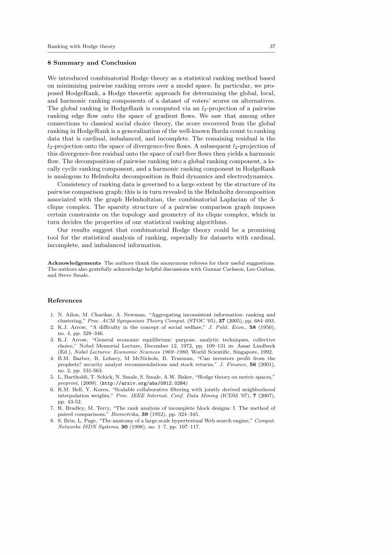
Ranking with Hodge theory 37
8 Summary and Conclusion
We introduced combinatorial Hodge theory as a statistical ranking method basedon minimizing pairwise ranking errors over a model space. In particular, we pro-posed HodgeRank, a Hodge theoretic approach for determining the global, local,and harmonic ranking components of a dataset of voters’ scores on alternatives.The global ranking in HodgeRank is computed via an l2-projection of a pairwiseranking edge flow onto the space of gradient flows. We saw that among otherconnections to classical social choice theory, the score recovered from the globalranking in HodgeRank is a generalization of the well-known Borda count to rankingdata that is cardinal, imbalanced, and incomplete. The remaining residual is thel2-projection onto the space of divergence-free flows. A subsequent l2-projection ofthis divergence-free residual onto the space of curl-free flows then yields a harmonicflow. The decomposition of pairwise ranking into a global ranking component, a lo-cally cyclic ranking component, and a harmonic ranking component in HodgeRankis analogous to Helmholtz decomposition in fluid dynamics and electrodynamics.
Consistency of ranking data is governed to a large extent by the structure of itspairwise comparison graph; this is in turn revealed in the Helmholtz decompositionassociated with the graph Helmholtzian, the combinatorial Laplacian of the 3-clique complex. The sparsity structure of a pairwise comparison graph imposescertain constraints on the topology and geometry of its clique complex, which inturn decides the properties of our statistical ranking algorithms.
Our results suggest that combinatorial Hodge theory could be a promisingtool for the statistical analysis of ranking, especially for datasets with cardinal,incomplete, and imbalanced information.
Acknowledgements The authors thank the anonymous referees for their useful suggestions.The authors also gratefully acknowledge helpful discussions with Gunnar Carlsson, Leo Guibas,and Steve Smale.
References
1. N. Ailon, M. Charikar, A. Newman, “Aggregating inconsistent information: ranking andclustering,” Proc. ACM Symposium Theory Comput. (STOC ’05), 37 (2005), pp. 684–693.
2. K.J. Arrow, “A difficulty in the concept of social welfare,” J. Polit. Econ., 58 (1950),no. 4, pp. 328–346.
3. K.J. Arrow, “General economic equilibrium: purpose, analytic techniques, collectivechoice,” Nobel Memorial Lecture, December 12, 1972, pp. 109–131 in: Assar Lindbeck(Ed.), Nobel Lectures: Economic Sciences 1969–1980, World Scientific, Singapore, 1992.
4. B.M. Barber, R. Lehavy, M McNichols, B. Trueman, “Can investors profit from theprophets? security analyst recommendations and stock returns,” J. Finance, 56 (2001),no. 2, pp. 531-563.
5. L. Bartholdi, T. Schick, N. Smale, S. Smale, A.W. Baker, “Hodge theory on metric spaces,”preprint, (2009). (http://arxiv.org/abs/0912.0284)
6. R.M. Bell, Y. Koren, “Scalable collaborative filtering with jointly derived neighborhoodinterpolation weights,” Proc. IEEE Internat. Conf. Data Mining (ICDM ’07), 7 (2007),pp. 43-52.
7. R. Bradley, M. Terry, “The rank analysis of incomplete block designs: I. The method ofpaired comparisons,” Biometrika, 39 (1952), pp. 324–345.
8. S. Brin, L. Page, “The anatomy of a large-scale hypertextual Web search engine,” Comput.Networks ISDN Systems, 30 (1998), no. 1–7, pp. 107–117.

38 X. Jiang, L.-H. Lim, Y. Yao, Y. Ye
9. S.-C. Choi, Iterative methods for singular linear equations and least-squares problems,Ph.D. thesis, Stanford University, Stanford, CA, 2006. (http://www.stanford.edu/group/SOL/dissertations/sou-cheng-choi-thesis.pdf)
10. S.-C. Choi, C.C. Paige, M.A. Saunders, “minres-qlp: a Krylov subspace method for indefi-nite or singular symmetric systems,” preprint, (2010). (http://arxiv.org/abs/1003.4042)
11. A.-N. de Condorcet, Essai sur l’application de l’analyse a la probabilite des decisionsrendues a la pluralite des voix, Imprimerie Royale, Paris, 1785.
12. F. Chung, Spectral graph theory, CBMS Regional Conference Series in Mathematics, 92,AMS, Providence, RI, 1997.
13. C. Cortes, M. Mohri, A. Rastogi, “Magnitude-preserving ranking algorithms,” Proc. In-ternat. Conf. Mach. Learn. (ICML ’07), 24 (2007), pp. 169–176.
14. H.A. David, The method of paired comparisons, 2nd Ed., Griffin’s Statistical Monographsand Courses, 41, Oxford University Press, New York, NY, 1988.
15. J.-C. de Borda, “Memoire sur les elections au scrutin,” Histoire de’Academie Royale desSciences, 102 (1781), pp. 657–665.
16. P. Diaconis, “A generalization of spectral analysis with application to ranked data,” Ann.Statist., 17 (1989), no. 3, pp. 949–979.
17. C. Dwork, R. Kumar, M. Naor, D. Sivakumar, “Rank aggregation methods for the web,”Proc. Internat. Conf. World Wide Web (WWW ’01), 10 (2001), pp. 613–622.
18. Y. Freund, R. Iyer, R. Shapire, Y. Singer, “An efficient boosting algorithm for combiningpreferences,” J. Mach. Learn. Res., 4 (2004), no. 6, pp. 933–969.
19. J. Friedman, “Computing Betti numbers via combinatorial Laplacians,” Algorithmica, 21(1998), no. 4, pp. 331–346.
20. T. Hastie, R. Tibshirani, “Classification by pairwise coupling,” Ann. Statis., 26 (1998),no. 2, pp. 451–471.
21. R. Herbrich, T. Graepel, K. Obermayer, “Large margin rank boundaries for ordinal re-gression,” pp. 115–132, Advances in large margin classifiers, MIT Press, Cambridge, MA,2000.
22. D. Hochbaum, A. Levin, “Methodologies and algorithms for group-rankings decision,”Manag. Sci., 52 (2006), no. 9, pp. 1394–1408.
23. A. Tahbaz-Salehi, A. Jadbabaie, “Distributed coverage verification in sensor networkswithout location information,” Proc. IEEE Conf. Decis. Control, 47 (2008), to appear.
24. M. Kahle, “Topology of random clique complexes,” Discrete Math., (2008), to appear.25. J.G. Kemeny, “Mathematics without numbers,” Daedalus, 88 (1959), pp. 571-591.26. J.G. Kemeny, L.J. Snell, “Preference ranking: an axiomatic approach,” pp. 9–23 in J.G. Ke-
meny and L.J. Snell (Eds.), Mathematical models in the social sciences, MIT Press, Cam-bridge, MA, 1973.
27. M.G. Kendall, J.D. Gibbons, Rank correlation methods, 5th Ed., Oxford University Press,Oxford, 1990.
28. M.G. Kendall, B.B. Smith, “On the method of paired comparisons,” Biometrika, 31(1940), no. 3–4, pp. 324–345.
29. J. Kleinberg, “Authoritative sources in a hyperlinked environment,” J. ACM, 46 (1999),no. 5, pp. 604–632.
30. M. Ma, “A matrix approach to asset pricing in foreign exchange market,” preprint, (2008).(http://ssrn.com/abstract=921755)
31. G.A. Miller, “The magical number seven, plus or minus two some limits on our capacityfor processing information,” Psychol. Rev., 63 (1956), no. 2, pp. 81–97.
32. J. Morton, L. Pachter, A. Shiu, B. Sturmfels, O. Wienand, “Convex rank tests and semi-graphoids,” SIAM J. Discrete Math., 23 (2009), no. 3, pp. 1117–1134.
33. F. Mosteller, “Remarks on the method of paired comparisons I, II, III” Psychometrika,16 (1951), no. 1, pp. 3–9, no. 2, pp. 203–218.
34. G.E. Noether, “Remarks about a paired comparison model,” Psychometrika, 25 (1960),pp. 357–367.
35. C.C. Paige, M.A. Saunders, “lsqr: an algorithm for sparse linear equations and sparseleast squares,” ACM Trans. Math. Software 8 (1982), no. 1, pp. 43–71.
36. D.G. Saari, V.R. Merlin, “A geometric examination of Kemeny’s rule,” Soc. Choice Welf.,17 (2000), no. 3, pp. 403–438.
37. T.L. Saaty, “A scaling method for priorities in hierarchical structures,” J. Math. Psych.,15 (1977), no. 3, pp. 234–281.
38. A.K. Sen, “The impossibility of a Paretian liberal,” J. Polit. Econ., 78 (1970), no. 1,pp. 152–157.

Ranking with Hodge theory 39
39. A.K. Sen, “The possibility of social choice,” Nobel Lecture, December 8, 1998, pp. 178–215in: Torsten Persson (Ed.), Nobel Lectures: Economic Sciences 1996–2000, World Scientific,Singapore, 2003.
40. L.L. Thurstone, “The method of paired comparisons for social values,” J. Abnorm. Soc.Psychol., 21 (1927), pp. 384–400.
41. Y. Xu, J.S. Dyer, A.B. Owen, “Empirical stationary correlations for semi-supervised learn-ing on graphs,” preprint, (2009).
42. H.P. Young, “Condorcet’s theory of voting,” Am. Polit. Sci. Rev., 82 (1988), pp. 1231–1244.
43. H.P. Young, A. Levenglick, “A consistent extension of Condorcet’s election principle,”SIAM J. Appl. Math., 35 (1978), no. 2, pp. 285–300.
44. J. Zhang, “Binary choice, subset choice, random utility, and ranking: a unified perspectiveusing the permutahedron,” J. Math. Psych., 48 (2004), no. 2, pp. 107–134.