NASA/TP--2002-212020

Statistical Properties of MaximumLikelihood Estimators of Power

Law Spectra Information

L. W. Howell

Marshall Space Right Center, Marshall Space Flight Center, Alabama

September 2002

https://ntrs.nasa.gov/search.jsp?R=20020079433 2020-04-21T04:15:59+00:00Z

The NASA STI Program Office...in Profile

Since its founding, NASA has been dedicated to

the advancement of aeronautics and spacescience. The NASA Scientific and Technical

Information (STI) Program Office plays a key

part in helping NASA maintain this importantrole.

The NASA STI Program Office is operated byLangley Research Center, the lead center for

NASA's scientific and technical information. The

NASA STI Program Office provides access to the

NASA STI Database, the largest collection of

aeronautical and space science STI in the world. The

Program Office is also NASA's institutional

mechanism for disseminating the results of itsresearch and development activities. These results

are published by NASA in the NASA STI Report

Series, which includes the following report types:

TECHNICAL PUBLICATION. Reports of

completed research or a major significant phaseof research that present the results of NASA

programs and include extensive data or

theoretical analysis. Includes compilations ofsignificant scientific and technical data and

information deemed to be of continuing referencevalue. NASA's counterpart of peer-reviewed

formal professional papers but has less stringent

limitations on manuscript length and extent of

graphic presentations.

TECHNICAL MEMORANDUM. Scientific and

technical findings that are preliminary or of

specialized interest, e.g., quick release reports,

working papers, and bibliographies that containminimal annotation. Does not contain extensive

analysis.

CONTRACTOR REPORT. Scientific and

technical findings by NASA-sponsored

contractors and grantees,

CONFERENCE PUBLICATION. Collected

papers from scientific and technical conferences,

symposia, seminars, or other meetings sponsored

or cosponsored by NASA.

SPECIAL PUBLICATION. Scientific. technical,

or historical information from NASA programs,projects, and mission, often concerned with

subjects having substantial public interest.

TECHNICAL TRANSLATION.

English-language translations of foreign scientific

and technical material pertinent to NASA'smission.

Specialized services that complement the STI

Program Office's diverse offerings include creating

custom thesauri, building customized databases.organizing and publishing research results...even

providing videos.

For more information about the NASA STI ProgramOffice, see the following:

• Access the NASA STI Program Home Page athttp://www.sti.nasa.gov

• E-mail your question via the Internet to

help@ sti.nasa.gov

• Fax your question to the NASA Access HelpDesk at (301) 621-0134

• Telephone the NASA Access Help Desk at (301)621-0390

Write to:

NASA Access Help Desk

NASA Center for AeroSpace Information7121 Standard Drive

Hanover, MD 21076-1320

NASA / TP--2002-212020

Statistical Properties of MaximumLikelihood Estimators of Power

Law Spectra Information

L. W. Howell

Marshall Space Flight Center, Marshall Space Flight Center, Alabama

National Aeronautics and

Space Administration

Marshall Space Flight Center • MSFC, Alabama 35812

September 2002

Acknowledgments

The author gives special appreciation to John Watts of the Cosmic-Ray Group, Space Science Department,

Marshall Space Flight Center, Huntsville, AL, for his many technical discussions and editorial remarks pertainingto this Technical Publication.

The author is grateful to Professor Herman J. Bierens, Professor of Economics, Pennsylvania State University,

and part-time Professor of Econometrics, Tilburg University, the Netherlands, for his assistance in checking equation (39)

in Appendix A----Closed-Form Expression for the Cramer-Rao Bound of the Broken Power Law.

TRADEMARKS

Trade names and trademarks are used in this report for identification only. This usage does not constitute an official

endorsement, either expressed or implied, by the National Aeronautics and Space Administration.

Available from:

NASA Center for AeroSpace Information712 ! Standard Drive

Hanover, MD 21076-1320

(301) 621-0390

National Technical Information Service

5285 Port Royal Road

Springfield, VA 22161(703) 487-4650

TABLE OF CONTENTS

1. INTRODUCTION ..........................................................................................................................

1.1 Simple Power Law Energy Spectrum ......................................................................................

1.2 Broken Power Law Energy Spectrum .....................................................................................

1.3 Break-Size 0.3 Study ...............................................................................................................

1.4 Analysis of Multiple Independent Data Sets ...........................................................................

1.5 Example of Estimating a 1 of a Simple Power Law Using Two Data Sets .............................

1.6 Using the CRB to Explore Instrument Design Parameters When Estimating

0=(o_ l, c_2, E/.) of a Broken Power Law Using Three Data Sets ..............................................

2. CONCLUSIONS ............................................................................................................................

APPENDIX A---CLOSED-FORM EXPRESSION FOR THE CRAMER-RAO BOUND

OF THE BROKEN POWER LAW .....................................................................................................

A. 1 Derivation ................................................................................................................................

A.2 Check on Equation (39) by Professor Bierens ........................................................................

APPENDIX B--CRAMER-RAO BOUND FOR MULTIPLE INDEPENDENT DATA SETS .......

REFERENCES ....................................................................................................................................

2

10

18

27

30

35

38

39

39

43

44

48

,°°

111

LIST OF FIGURES

.

3.

.

.

.

.

3.

9.

10.

11.

Mean estimates of O:ML as a function of the number of events, N, showing

a bias for N<I,000. Triangle marker at N = 200 and 52,000

is for method of moments ....................................................................................................

Standard deviation of O_ML and the CRB as a function of N ................................................

MLE and method of moments as a function of instrument energy resolution

for the proposed TSC with Gaussian response function ......................................................

Frequency histograms of aML for 10,000 simulated missions with (a) N = 50

and (b) N = 52,000 events, using the TSC with its 40-percent resolution

Gaussian response function ..................................................................................................

Frequency histogram of aML based on 10,000 simulated missions with N = 50

using an ideal detector. The smooth curve is the theoretical distribution of O_ML

obtained from equation (13) .................................................................................................

Standard deviation of the ML estimator aML versus N for a 40-percent

resolution Gaussian detector based on 10,000 simulated missions at each

value of N and the CRB for the 40-percent Gaussian detector computed

with equation (14) (_) The CRB for the ideal detector is included

as a reference curve (-- --) ...................................................................................................

CRB as a function of N for detector resolutions in the range 0 < __ 0.40.

The proposed TSC instrument with its expected 52,000 events is indicated

by the square and the observing energy range was set to 20-5,500 TeV ............................

ML estimate of a I and _, as a function of detector collecting power .................................

ML estimate of E_: as a function of detector collecting power using 40-percent

resolution Gaussian response function (the TSC) and the ideal detector. The knee

location E k was set to 100 TeV in these simulations ...........................................................

CRB of a I using TSC (-- --) and ideal detector (_) obtained from equation (20)

versus collecting power. Standard deviations of ML estimates from simulations for

values of N in table 1 indicated by markers .........................................................................

CRB of _, using TSC (-- --) and ideal detector (_) obtained from equation (20)

versus collecting power. Standard deviations of ML estimates from simulations for

values of N in table 1 indicated by markers .........................................................................

9

10

12

13

14

15

iv

LIST OF FIGURES (Continued)

12.

13.

14.

15.

16.

17.

18.

19.

20.

21.

22.

23.

CRB of E_ using TSC (-- --) and ideal detector (_) obtained from equation (20)

versus collecting power. Standard deviations of ML estimates from simulations for

values of N in table 1 indicated by markers .........................................................................

Relative frequency histograms of the ML estimate of a 1 (leftmost two histograms)

for N = 11,439 (broadest of the two) and N = 114,390 (narrow histogram).

Rightmost two histograms similarly defined for ¢Y-2_............................................................

Relative frequency histograms of the ML estimates of E k for N = 11,439 (broadest

of the two and with bump in fight-hand tail) and N = 114,390 ............................................

Relative frequency histograms of ML estimates of a I and oc2_for N = 22,877

and N 2-- 1,000 .....................................................................................................................

ML estimate of a I and _ as a function of detector collecting power when the spectralbreak size is 0.3 for the TSC and ideal detector ...................................................................

ML estimate of E k as a function of detector collecting power using the TSC

and ideal detector when the break size is 0.3. The actual concept TSC with

its expected N -- 51,790 events is indicated by the diamond and is based on

25,000 simulated missions (others are 5,000 missions each) and suggests the

marker to its immediate right is probably a little on the high side .......................................

CRB of a I using TSC (-- -) and ideal detector (_) versus collecting power.Stand deviations of ML estimates from simulations for values of N in table 2

indicated by markers ............................................................................................................

CRB of a 2 using TSC (-- --) and ideal detector (_) versus collecting power.Standard deviations of ML estimates from simulations for values of N in table 2

indicated by markers ............................................................................................................

CRB of E k using TSC (-- -) and ideal detector (_) versus collecting power.Standard deviations of ML estimates from simulations for values of N in table 2

indicated by markers ............................................................................................................

Relative frequency histograms of ML estimates of o_l and _ for the proposed TSC .........

Relative frequency histograms of the ML estimates of E k for the proposed TSC ...............

Objective function given by equation (18) for the ideal detector in the neighborhood

of 0ML for a simulated mission, keeping a I fixed at the ML estimate. There were

114,385 (4,819) events in this mission. The vertical axis has been scaled to 1 ...................

15

16

17

17

18

19

20

20

21

21

23

LIST OF FIGURES (Continued)

24. Contour plot of the objective function for ideal detector in the neighborhood of 0ML

for a simulated mission, keeping a 1 fixed at the ML estimate. There were 114,385

(4,819) events in this mission ............................................................................................... 24

25. Objective function for ideal detector in the neighborhood of 0ML for a simulated

mission, keeping a I fixed at the ML estimate. This mission consisted of 4,575

(207) events. The vertical axis has been scaled to 1 ............................................................. 25

26. CRB used to estimate where the distribution of tz2_begins to cross that of a I

when (a) the spectral break size is 0.5 and (b) the spectral break size is 0.3 ....................... 26

27a. ML estimates of (Z l for 25 missions, with E l = 5 TeV (5,275 events for TRD

and 593 for calorimeter) ....................................................................................................... 31

27b. ML estimates of a I for 25 missions, with E t = 3 TeV ( 11,660 events for TRDand 593 for calorimeter) ....................................................................................................... 32

27c. ML estimates of a 1 for 25 missions, with E 1 = 1 TeV (56,920 events for TRD

and 593 for calorimeter). Note that ObrR D and aBoth are virtually indistinguishable ........... 32

28. Gamma, Gaussian, and broken Gaussian detector response functions

to 40-TeV proton .................................................................................................................. 36

vi

LIST OF TABLES

1. Number of events used in broken power law simulations 0.5 break-size study ................... 12

'3 Number of events used in broken power law simulations for 0.3 break-size study .............. 18

. Summary statistics based on 25,000 simulated missions, 0 = (2.8, 3.1, 100 TeV)

and observing range 20-5,500 TeV, for the TSC having Gaussian response function ........,.) ,-)_m

. Effect of lowering E I on the CRB for the TSC-sized detector with 0-, 20-,

and 40-percent resolution Gaussian response function. The number

of events N 2 above E k is 2,255 for all values of E l ............................................................... 27

5. Summary statistics of _Cal based on 1,000 simulated missions of the calorimeter .............. 33

. Summary statistics of t_61-RD based on 1,000 simulated missions for each value of E 1

of the TRD alone (all events between E l and 20 TeV) ......................................................... 33

, Summary statistics of O_Both based on 1,000 simulated missions for each value of E t

of the TRD and calorimeter acting in combination ............................................................... 33

. Data sets and associated response functions, with CRB for all possible

combinations of data sets ...................................................................................................... 35

9. Number of events from table 4 in data set C is increased by a factor of 10 ......................... 36

10. Number of events from table 4 in data set B is reduced by a factor of 2

and those in C increased by a factor of 10 ............................................................................ 37

11. Number of events from table 4 in data set B is reduced by a factor of 2

and those in C increased by a factor of 10, resolution of A improved

to 30 percent and C to 35 percent .......................................................................................... 37

vii

LIST OF ACRONYMS

CRB

EE

GCR

GEANT

ML

MLE

rl

TP

TSC

Cramer-Rao bound

errant estimate

galactic cosmic ray

GEometry ANd Tracking particle physics simulation program

maximum likelihood

maximum likelihood estimation

radiation length

Technical Publication

thin sampling calorimeter

°°°

VIII

NOMENCLATURE

E

I

L

0

Z

energy (units in TeV)

information matrix

likelihood function

objective function

standard normal random number

ix

TECHNICAL PUBLICATION

STATISTICAL PROPERTIES OF MAXIMUM LIKELIHOOD ESTIMATORS

OF POWER LAW SPECTRA INFORMATION

1. INTRODUCTION

A brief summary of the maximum likelihood estimation (MLE) procedure developed for estimating

power law spectral parameters in earlier worksl.2 begins with the probability density function of the

astrophysics data set consisting of N detector responses Yi, e.g., energy deposit, as

g(yi;O)= [ g(Yi I E;p)(P (E;O)dE, i= l,...,N ,

R

(1)

where 0 denotes the vector of spectral parameters of an assumed energy spectrum 0(E,'0) to be estimated;

N is the number of detected events from observing range, R, of the instrument having response function, g,

and energy resolution, p. Then the corresponding likelihood function is

L(0) = g(Yi [E;p) (p(E;O)dE

i=1 L R

(2)

and the ML estimate of 0, say 0ML, is chosen so that for any admissible value of 0, L(0ML)- > L(0) or

equivalently, Iog[L(0ML)] > log[L(0)]. 3 In practice, 0ML can be obtained from equation (3) using an opti-

mization routine, such as the Nelder-Meade simplex search algorithm, 4 to yield

OML = minO(O) , (3){o}

where the objective function, O, in equation (3) is defined as O(0) = -log[L(0)] for this minimization

algorithm so that minimizing O(0) maximizes log[L(0)] as desired, and where the integral appearing in

equation (2) and thus intrinsic to equation (3) can be very accurately evaluated by numerical methods such

as the method of Gaussian quadratures. 5 The Nelder-Mead algorithm does not require gradient information

which is a vital consideration in selecting an optimization algorithm for this application because some

energy spectra, such as the broken power law, are not differentiable everywhere.

The MLE theory generally leads to lower bounds on the statistical errors (standard deviations) of

the spectra information and the existence of such a bound, called the Cramer-Rao bound (CRB), is the

bound below which the variance of an unbiased estimator cannot fall. This implies that irrespective of the

method used to quantify the parameters from the data, there is a lower bound on the precision that cannot

be superseded. 6 In the multiparameter case, if 0 is any unbiased estimator of O, then

[. /Olog[g(y;O)] Olog[g(y;O)]\] -1

var(0)_>[_v\ _-0 × _0 T /j(4)

in the sense that the difference of these two matrices is positive semidefinite. The right-hand-side matrix in

equation (4) is the CRB 7 and notationally will be referred to as I-lie), where I(0) is frequently called the

information matrix; the notation <. > denotes "expected value"; and the superscript T stands for vector

transpose. Thus, the variance of one component of is tt say 0/, is bounded below as var(0i) _ I_ 1(0), where

1_ I (e) is the ith diagonal element of 1-1 (e). When 0 consists of a single spectral parameter, e.g., a simple

power law energy spectrum is assumed, the CRB is the right-hand side of the inequality

var(O) >

N/(Ol°g[g(y;O)]]2 I

) /(5)

Additionally, ML estimators generally possess the favorable large sample properties of consistency

(unbiased) (PI) and normality (P3). 6,8.9 This Technical Publication (TP) investigates the conditions whereby

these two properties, along with efficiency which is attainment of the CRB and is referred to as property P2

in this TP, are attained for an assumed simple power law energy distribution and a broken power law

distribution, with emphasis on practical applications to instrument design and data analysis.

1.1 Simple Power Law Energy Spectrum

The simple power law suggests that the number of protons detected above an energy, E, is given by:

-Ofl +1NS(> E)= M A (6)

where E is in units TeV, a 1 is believed to be =2.8, and M a and EA are numbers associated with the detector's

collecting power (combination of size and observing time). In statistical terms, N s is assumed to represent

an average number of events, while the actual number to be observed on any given mission would follow

the Poisson probability distribution with mean number N S. The probability density function for galactic

cosmic ray (GCR) event energy, E, is then given by

0

O_1 -- 1

(_s(E) = -al _l_a I E -at for E 1 <_ E < E 2E l -L 2

(7)

over an energy range [E l, E2] that does not depend on the parameter a 1. Because the actual incident

particle energies are never observed, but only a measure of their energy deposition from their passage

through the detector, the random variable Y is introduced to represent the detector's response, e.g., energy

deposition, of a GCR proton of incident energy, E, and its stochastic response function, g, with energy

resolution, p, which may or may not be energy independent. For specificity, a response function, g, based

on simulation studies of a thin sampling calorimeter (TSC) concept for the Advanced Cosmic-Ray Compo-

sition Experiment for the Space Station (ACCESS) will be used. It has a planned 3-yr program life cycle

and is composed of a carbon target and sampling calorimeter. The TSC area is 1 m 2 with a target =0.7

proton interaction lengths thick, sampled by .Z/Y pairs of square scintillating fibers. The fibers in the target

are 2 mm thick and provide the approximate position of the interaction. The calorimeter consists of upper

and lower parts totaling 25 radiation length (rl)-thick lead and contains 28 X/Y pairs of 500-_m square

scintillating fibers. The upper 3-rl-thick calorimeter is sampled each 0.5 rl, and the lower part is sampled

each 1.0 rl. The total weight of the target and calorimeter is =2,600 kg, and the collecting power param-

eters, M a and E a are estimated to be 160 and 500 TeV, respectively, implying that this TSC is expected to

observe 160 proton events above 500 TeV over its expected 3-yr life cycle.

The TSC performance predictions are based on the geometry and tracking particle physics simula-

tion program (GEANT) simulations of energy deposition for monoenergetic protons at specified energies

at 0.1, 1, 10, 100, 1,000, and 5,000 TeV for this candidate detector. The Gaussian distribution was found to

provide a reasonable description of the distribution of energy depositions at each of these incident ener-

gies. 1° The mean detector response and the rms response were both found to be well approximated by a

linear function of incident energy, E, in the range of interest for this study, which is typically in the range of

20 to 5,500 TeV. Thus, the mean energy deposition, Y, for a given incident energy, E, is defined to be/.ty1E

= (a + bE) and the rms response defined as CrrlE = (c + dE), where the coefficients a, b, c, and d wereestimated from the GEANT simulation results.

Before investigating the properties of MLE for the TSC instrument, it is instructive to consider the

concept of a zero-resolution instrument or so-called ideal detector because it sets an upper bound on the

expected performance of any real detector of equal collecting power. This measurement bound is deter-

mined by the CRB for the ideal detector which in turn establishes the limit in attainable precision with

which unbiased spectra information can be obtained from a given science mission by any conceivable

instrument with equal or less collecting power. Hence, it is useful in crafting realistic measurement goals

for new science missions. Thus, the true character of the energy spectrum can be studied using an ideal

detector without the additional statistical variations induced by real detectors, which is valuable when

considering real detectors.

An ideal detector's energy resolution, p, is equal to zero, so the standard deviation _YYIEis zero for

all GCR event energies, E. Hence, the incident GCR energies are precisely known from the inverse mean

response, so that for the TSC having linear mean response gives E = (Y- a)/b, and using equation (5)

provides the CRB as the right-hand side of the inequality:

var(&) _> 1

(a I - 1)2 El+atE_+a----_l(1--°g[E'_]-(E,.,E_-El E_at )2"-- l°--g[El ])21/(8)

and is asymptotically attained by the ML estimator. A key question then arises, "For what values of N is this

asymptotic property P2, as well as PI and P3, achieved by MLE?" A battery of simulations was conducted

to study this question consisting of 10,000 simulated missions for each of several values of N ranging from

50 to 52,000* events per mission and with GCR energies from the energy range of 20 to 5,500 TeV. The

ML estimate aML was obtained for each mission by solving

0log[L] 1

_a I a I - 1

log[E2]/:_ -log[E l] E l al 1 N- - log[Ei ] = 0

/:2

(9)

in terms of a I for the ideal detector and then also for a 40-percent resolution Gaussian detector (the TSC)

by application of equation (3). For comparison, the estimation technique referred to as the "method of

moments" is included for the ideal detector (p = 0) for the case N = 200 events and N = 52,000 events, and

consists of equating the sample mean E to the population mean as

tz2

(10)

and then solving the nonlinear equation (10) in terms of &1.2 Figure 1 shows that MLE provides an unbi-

ased estimate of a ! when N > 1,000, but with an ever-increasing bias as the number of events diminishes.

Note that even though aML is biased when N = 200 for the 40-percent resolution Gaussian TSC, its bias is

significantly less than the bias of the method of moments estimator 41 for the ideal detector having perfect

energy resolution.

An analytical expression that allows one to compute the bias of 0tML for the ideal detector can be

constructed by noting in equation (9) that aML is a function of the logarithm of the event energies by the1 ,v

term _'2_:j log[Ei]. Thus, the random variable W = log[E] is introduced having probability density

function

(CzI - I)EI1 t_,_-aie w(l-Oq )f(w)= - , log[El]<w<log[E2] (11)

Ei Ea' - El' E2

*The TSC used in the ACCESS concept study would detect 52,000 events on average over the energy

range of 20 to 5,500 TeV when the spectral parameter, a 1, is assumed to be 2.8.

4

m

E.w

....I

41, Ideal Detector

• Method of Moments (Ideal)

D 40% Resolution, Gaussian

Theoretical Mean (Ideal Detector)

_.J

2.88

LJ2.87

2.86

2.85

2.84

2.83

2.82

2.81

2.80

2.7910

r-,_3

mira

I I I I

100 200 1,000 10,000 100,000

Number of Events

Figure 1. Mean estimates of O_ML as a function of the number of events, N,

showing a bias for N<1,000. Triangle marker at N = 200 and 52,000

is for method of moments.

and with mean and variance

law = log[El] 41 E1 _E,82

t--1 + oq co

_V-1 E? 1E282 E1 °q E_ 52

(12)

1 N

where 6= log[ El]- log[ E2 ], co= -E_' E 2 + E l E_', and, by the central limit theorem, _y__ w/is nor-

1

mally distributed with mean Pwand variance __Y_V • Consequently, the probability distribution of the ML

estimator aML of a I using the ideal detector is obtained by solving the probability equation,

Pr,

l -log[E2] E_ -a_ -log[E]] El -as_

aML- 1 - ]-'Uw < Zi .v2

1

= ---_-_e 2dx ,--oo

(13)

in terms of O_ML for various values of Z. Letting Z vary from -5 to 5, setting N to each of the number of

events N used in figure 1, and then numerically evaluating the mean of aML from the probability density

function constructed from equation (13) gives the solid curve shown in figure 1, indicating good agreementwith the simulation results.

An interesting observation from figure 1 is that one would likely conclude, and incorrectly, is that a

significant difference between the slopes of two cosmic-ray elemental species exists if their respective

number of events were significantly different from each other and at least one had fewer than 1,000 events.

This is because for two given cosmic-ray elemental species, A and B, with simple power law parameters, o_

and/3, the hypothesis H0: _-/3 = 0 (same "slopes") versus/-/l:a- fie 0 uses the test statistic aML -/3ML

that will inherit the bias(s) shown in figure 1 when N is < 1,000. Thus, an interesting study would be to plot

the estimate of the slope parameter for each of several elemental species as a function of Ncomprising their

respective data sets to see if it resembles figure 1. It should also be understood that this bias as a function of

N would be even worse had the method of moments estimation procedure been used to estimate the spectral

parameters as previously noted in figure 1.

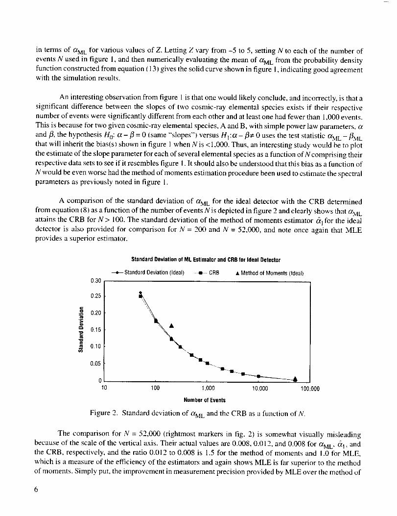
A comparison of the standard deviation of O_ML for the ideal detector with the CRB determined

from equation (8) as a function of the number of events N is depicted in figure 2 and clearly shows that _ML

attains the CRB for N > 100. The standard deviation of the method of moments estimator &l for the ideal

detector is also provided for comparison for N = 200 and N = 52,000, and note once again that MLE

provides a superior estimator.

ce.i

t_

"5

t_

Standard Deviation of ML Estimator and CRB for Ideal Detector

0.30

Standard Deviation (Ideal) --_m--- CRB • Method of Moments (ideal)

0.25

0.20

0.15

0.10

0.05

010

A

\

I I

100 1,000 10,000 100 000

Number of Events

Figure 2. Standard deviation of O_ML and the CRB as a function of N.

The comparison for N = 52,000 (rightmost markers in fig. 2) is somewhat visually misleading

because of the scale of the vertical axis. Their actual values are 0.008, 0.012, and 0.008 for aML, &l, and

the CRB, respectively, and the ratio 0.012 to 0.008 is 1.5 for the method of moments and 1.0 for MLE,

which is a measure of the efficiency of the estimators and again shows MLE is far superior to the method

of moments. Simply put, the improvement in measurement precision provided by MLE over the method of

6

moments can be roughly equated to doubling the collecting _ower of the instrument, because doubling the

collecting power reduces the standard deviation by 1/V2 when the CRB is attained. Furthermore,

this ratio of = 1.5 remained steady as the detector resolution varied from zero to 50 percent, as shown in

figure 3. This fact, coupled with the better performance in achieving P1 as previously discussed, explains

why MLE is superior to the method of moments when estimating power law spectra information.

0.016

E 0.012,c#)

tiLl

c

.o_ 0.008

0.004

f..

0

Figure 3.

ML EstimatorOr.ML, Methodof MomentsEstimator,andCRBVersusDetectorEnergyResolution.

N=-52,000Events

• Method of Moments [] Maximum Likelihood CRB

41,

I I

0 20 40 60

DetectorResolution(%)

MLE and method of moments as a function of instrument energy resolution

for the proposed TSC with Gaussian response function.

Property P3 is investigated using a frequency histogram of O_ML based on the 10,000 simulated

missions when N -- 50 events per mission and shows a significant right-hand skewness (fig. 4a), and thus,

a clear departure from normality (Gaussian fit is illustrated as smooth curves in fig. 4), while a similar

comparison for the case N = 52,000 shows aML is very normally distributed. Visual studies of the interme-

diate values of N showed the frequency histograms to be normally distributed in appearance for N_> 1,000 and

is in concert with the bias study depicted in figure 1.

Histogramof ML Estimateof (_1With GaussianFit,GaussianDetector, N= 50

50

40¢D

ao

_ 20

t_

(a)

10

02

m

2.5 3 3.5 4 4.5

ML Estimateof (](1

Histogramof ML Estimateol a_ With GaussianFit,GaussianDetector, N= 52,000

50

40

g 30

_ 20

_ to

02.75 2.85

ML Estimate ofa_(b)

Figure 4. Frequency histograms of O_ML for 10,000 simulated missions with (a) N = 50

and (b) N = 52,000 events, using the TSC with its 40-percent resolution Gaussian

response function.

A relative frequency histogram of aML based on 10,000 simulated missions with N = 50 per mis-

sion using an ideal detector having zero energy resolution is shown in figure 5. Also shown is the theoreti-

cal distribution of aML obtained from equation (13) with parameters set to N = 50, E l = 20 TeV, E 2 = 5,500

TeV, and a I = 2.8 and illustrates the close agreement between simulation and theory.

Histogram of ML Estimate of O_ 1 With Theoretical Distribution When N= 50 for the Ideal Detector

2.0

1.6

._ 1.2

.__

_m 0.8iw

IX

0 I I

2 4 4.5 5

0.4

2.5 3 3.5

Figure 5.

aML

Frequency histogram of O_ML based on 10,000 simulated missions with N = 50

using an ideal detector. The smooth curve is the theoretical distribution of O_ML

obtained from equation (13).

Solving equation (3) to obtain the ML estimate for the case where the events are measured by a real

detector having nonzero energy resolution is straightforward, and checking consistency (PI) and normality

(P3) is easily performed. However, checking efficiency (P2) can be quite formidable because of the term

\/ = log g(Y IE,p) Os(E;al )dE g(Y IE,p) q_s(E;_l )dE dy

JJ EEl

(14)

required to compute the CRB, coupled with the fact that the detector response function, g, in equation (14)

can be quite complicated. For example, g could be Gaussian with non-negativity constraint 3' > 0 and

energy-dependent resolution function, p(E), that in turn requires an energy-dependent normalizing coeffi-

cient. Fortunately, equation (14) can be numerically evaluated using the symmetrized form of the numeri-cal derivative, 1t

f'(x)= f(x + 17)- f(x- h) (15)2tl

to approximate the derivative in equation (14) and in conjunction with the method of Gaussian quadratures

to calculate the definite integrals. The fact that the CRB in equation (8) for the ideal detector must match

the CRB obtained from equation (14) when the detector resolution is zero (p---_0) provides a means to tune

the numerical differentiation parameter, h, and the integration parameters, e.g., the upper integration limit

for y as well as the number of partitions used in the numerical integration in both integration variables, E

and 3; in equation (14). For the TSC instrument with a data analysis range of 20 to 5,500 TeV, setting h to

0.0001 and the upper integration limit of y to 35,000 GeV in place of infinity in equation (14), and using

10-point Gaussian quadratures over subintervals over both integration ranges provides the somewhat sur-

prising result of 13-decimal-place accuracy in the numerical evaluation of equation (14) when compared to

the exact value obtained from equation (8) for the ideal detector. This accuracy in the numerical evaluation

of equation (14) was independently confirmed using the numerical integration routine in MATHEMATICA ®.

Figure 6 illustrates the convergence of the standard deviation of the ML estimator aML to the CRB

computed using equation (14) for a 40-percent resolution Gaussian detector as a function of N. The stan-

dard deviation of t_ML is based on a battery of 10,000 simulated missions for each value of N, where N

ranges from 50 to 52,000 events per mission. The CRB for the ideal detector is included as a reference

curve (--).

o

t_

t--

0.4

0.3

0.2

0.1

• Standard Deviation (40% Gaussian) _ CRB(40% Gaussian) --- CRB(Ideal)

N

\\

0 I I

10 100 1,000 100,000

Number o! Events

Figure 6. Standard deviation of the ML estimator aML versus N for a 40-percent resolution

Gaussian detector based on 10,000 simulated missions at each value of N and the

CRB for the 40-percent Gaussian detector computed using equation (14) (_).

The CRB for the ideal detector is included as a reference curve (-- - ).

When MLE is being used in the design phase of an instrument to estimate its expected performance

and if the simulations indicate that MLE does in fact provide unbiased spectra information and approxi-

mate attainment of the CRB for the science mission under study, then equation (14) can be used to evaluate

the relative merits of various instrument design parameters without performing additional simulations.

This has tremendous practical value in design parameter trade studies because equation (14) can be evalu-

ated in mere seconds, while the equivalent information from Monte Carlo simulations can take several

days. For example, because we know (from Fig. 2) that MLE attains the CRB for N > 100 events, equation

(14) can be used to compute the family of curves shown in figure 7 that relate the precision with which a l

can be measured as a function of detector resolution and collecting power. This implies instrument design-

ers should first attempt to maximize collecting power and then improve resolution, and in that order. The

proposed TSC instrument, with its expected 52,000 events, is indicated by the square in figure 7. The reader is

referred to figure 3 for a detailed view of the CRB calculated using equation (14) for the TSC as a function

of detector energy resolution.

9

0.25

CRBfora1UsingGaussianDetector,0%-40%Resolution

Figure 7.

¢J

0.20

0.15

0.10

0.05

0100

k

x,',:,,

1,000 10,000 100,000

NumberofEvents

--- 40%---- 30%

20%--- 10%.... 0%

CRB as a function of N for detector energy resolutions in the range 0 <p <0.40.

The proposed TSC instrument with its expected 52,000 events is indicated by the

square, and the observing energy range was set to 20-5,500 TeV.

A detailed simulation study of the TSC-sized ideal detector, with its expected N = 52,000 events for

the observing range 20-5,500 TeV and with a I = 2.8, was conducted and aML obtained from equation (9)

for each of i million missions (each mission detected 52,000 events), yielding a mean and standard devia-

tion value of aML to be 2.80003 and 0.007905, respectively. Constructing the probability density function

of aML from equation (13) and then numerically evaluating its mean and standard deviation gives 2.80003

and 0.007911, respectively, while the CRB calculated from equation (8) gives 0.00790998, illustrating the

remarkable agreement between simulation and theory and attainment of P2. Note that aML is essentially

unbiased too and thus, Pi is approximately attained. Because 5.2 × 1010 random numbers were required for

this 1-million simulated missions study, it is crucial to use a random number generator having a period

longer than 5.2 × 1010, such as the generator used in this study which has a period of =1018.

1.2 Broken Power Law Energy Spectrum

The broken power law energy spectrum suggests a transition from spectral index a I below the knee

location at energy E k to a steeper spectral index _2_> al above the knee.* The broken power law spectrum

predicts that the number of protons detected above an energy, E, is given by:

*The case a_ < a I and where E k is referred to as the ankle can also be handled by this MLE procedure.

l0

NB(> E)=

NS(> E)-[Ns(> Ek)-NB(> Ek)]

for E > E k

for E < E k

(16)

where E is in units TeV, M A and E a are 160 and 500 TeV, respectively, as before for the TSC instrument,

Ns(>E) is defined in equation (6), and currently available measurements suggest that a i is =2.8, or.2_is

thought to be somewhere between 3.1 and 3.3, and E k is parameterized in the range of 100 to 300 TeV for

this study. The broken power law probability density function 40B is obtained by normalizing N B over an

observing range [Et. E 2] of interest and is defined in equation (21 ) of appendix A.

The likelihood function of a random sample of N Galactic Cosmic Rays (GCR) events from the

broken power law spectrum detected by the ideal detector having perfect energy resolution, regarded as a

function of the unknown vector of parameters 0 = (a 1, ___, Ek), is

/L(O)= A(o)N H H -'

Ei<E k Ej>-Ek

E l <_ E i, Ej < E 2(17)

where the first product is over the event energies below the knee location E k and the second product is over

those event energies above E k, and they total in number to N, and A(0) is the normalizing coefficient given

in equation (22).

The Nelder-Mead simplex method can then be used to obtain 0ML from equation (18), where the

objective function O(0) is defined as minus the log-likelihood function, so that

{ 0}[ tEi<E_ _Ej>_E k

(18)

for N events detected by the ideal detector, while equation (2) must be used to construct the likelihood

function for a real detector having response function, g, and energy resolution, p, with N instrument

responses Yi • Consequently, the ME estimate 0ML is

OML = min -log{o}

(19)

where the range of inte_ation must be split at E k at each step in the simplex search for 0ML = (0¢ 1, O_2, Ek)ML.

11

To numericallyexplorethepropertiesof 0ML for the broken power law distribution, the vector of

spectral parameters is first set to 0 = (2.8, 3.3, 100 TeV) and events simulated from the energy range 20 to

5,500 TeV for each of several values of N selected so as to provide an average of 500, 1,000 ..... 5,000

events above E k as shown in table I. The notation N 2 is introduced to denote NB(>Ek), N for NB(>EI) so

that N 1=N-N2, and the notation N(N2) means "a total of N events, of which N, of them are above the

spectral knee Ek."

Table 1. Number of events used in broken power law simulations for 0.5 break-size study.

N1 10,939 21,877 32,816 43,754 65,631 87,508 109,390

N_ 500 1,000 1,500 2,000 3,000 4,000 5,000

N 11,439 22,877 34,316 45,754 68,631 91,508 114,390

For each value of N in table 1, 10,000 missions were simulated and for each of these missions, 0ML

was obtained using equation (18) for an ideal detector and equation (19) for the TSC detector having

Gaussian response function g and constant 40-percent energy resolution over the simulated energy range of20 to 5,500 TeV.

Figure 8 depicts the mean of the ML estimates of o_1 and (x2_versus the number of events N used in

the simulations and shows that when the collecting power of the detector provides > 1,500 events above Et.

(corresponding to third set of markers from left), property PI is essentially attained by the TSC instrument

since the relative bias is <3 percent for the 40-percent resolution Gaussian detector, and is even better for

the ideal detector having zero energy resolution.

Similarly, figure 9 illustrates the bias (recall Ek= 100 TeV in these simuations) of the ML estimate

of E k as a function of N for the TSC instrument and the ideal detector. Note that property PI is again

roughly attained by the TSC (relative bias is _<2 percent) when there are >1,500 events above E k.

t_

a_

m

E

,...I

3.4

a 1 (Ideal)

a t (40% 6aussian)

-.m-- a 2 (Ideal)

a 2 (40% Gaussian)

3.3

3.2

3.1

3.0

2.9

2.8 _

2.7

10,000

ii ,, A

A A A

I I I I I

30,000 50,000 70,000 90,000 110,000

Total Number ol Events N

Figure 8. ML estimate of a I and __ as a function of detector collecting power.

l')

110

Ek(Ideal) --!.- Ek(40%Gaussian)

_" 108

_ 106104

g 102m

_ 100

98

96 t i t J10,000 30,000 50,000 70,000 90,000

v

I

110,000

TotalNumberof EventsN

Figure 9. ML estimate of E k as a function of detector collecting power using a 40-percent

resolution Gaussian response function (the TSC) and the ideal detector.

The knee location E k was set to 100 TeV in these simulations.

Next, property P2 is investigated and requires the construction of the 3-by-3 information matrix

I(0). Equation (32) of appendix A provides I(0) for the ideal detector, while for a real detector with

response function, g, and energy resolution,/9, the/j-element of I(e) is, by equation (4),

I,_i(0) = c30i

×[E!g(y'E,P)(PB(E;O)dE]dv

I ]lO log g(yl E,P)(Pe(E;O)dE

L E ,

(20)

and can be accurately computed using the numerical methods discussed in the simple power law section,

and where the notation in equation (20) defines 01 --a 1, 02--__, and 03-E k, and where the integration range

[El, E2] must be split at E k for the inner three integrals.

A comparison of the CRB obtained from equation (20) for a 1 using the TSC with its 40-percent

Gaussian response function with the simulation results is shown in figure 10. Note the CRB is attained

when the number of events above the knee location is >1,500. The case 11,439 (500) had several simulated

missions in which the MLE procedure gave an estimate eML of 0 that suggests a simple power law would

probably be an adequate explanation of the simulated events. These Errant Estimates were characterized as

EEl ) E k and __ are both very large relative to their assumed values of 100 TeV and 3.3 in the simulations,

13

andEE2)E k and a I are both very small. While the condition a I = (x2 is normally associated with suggest-

ing a simple power law adequately fits the data, these unlucky missions illustrate the beauty of the MLE

procedure in finding two other conditions whereby a broken power law collapses into a simple power law.

The first condition is a broken power law with E k above the range of detected events and a_---_oo in an effort

to explain the absence of events above E k, which is indeed just a simple power law over the range of

detected events and implied by EEl. The second condition is a broken power law with E k below the range

of detected events and al---_0 and implied by EE2. Eliminating these errant estimates of a I gives the

trimmed standard deviation depicted at N = 11,439 (and N 2 = 500) in figure 10 and symbolized by a filled

circle on the plot. The CRB for the ideal detector calculated from equation (42) is also shown in figure 10

with corresponding simulation results. Additionally, the difference between the covariance matrix of the

ML estimates and I-l(e) was noted to be positive definite as each its three eigenvalues were positive, with

two of them approximately zero for all values of N in table 1 used in the simulations.

Similar results are illustrated in figure 11 for (x2 and figure 12 for E k. Trimmed estimates for these

two make little difference because of their already larger variance relative to that of a I .

0.08

StandardDeviationof MLEstimateof a 1 andCRB

A o (ideal) _ CRB(Ideal) • Trimmed

II o (40%Gaussian) mm CRB(40%Gaussian)

0.07

0.06

"_ 0.05Em 0.04

t--

ml

%\m

0'03I__. I1...0.02 "_4L"L -"- ...ql..- ..._ ....

0.01_ -4-- ---..._ '--II/

0 / I I I t I

10,000 30,000 50,000 70,000 90,000 110,000

TotalNumberof EventsN

Figure 10. CRB of a I using TSC (-- - ) and ideal detector (_) obtained from equation (20)

versus collecting power. Standard deviations of ML estimates from simulations for

values of N in table 1 indicated by markers.

14

c-o

m

Figure 11.

0.25

StandardDeviation of ML Estimateof a z and CRB

• G(40% Gaussian) ---- CRB(40% Gaussian)

,Lo (Ideal) _CRB (Ideal) oTrimmed

0.20 _

0.15 &_,_, S

o. oI _ __0.05 [ _ .I. ,a.

/O/ L i i L i

10,000 30,000 50,000 70,000 90,000 110,000

Total Numberof EventsN

CRB of _ using TSC (-- -- ) and ideal detector (_) obtained from equation (20)

versus collecting power. Standard deviations of ML estimates from simulations for

values of N in table 1 indicated by markers.

4o

StandardDeviation of ML Estimateof Ekand CRB

s ok (40% Gaussian) m_ ORB(40% Gaussian) ,LOk(Ideal) CRB(ideal)

m35 -

30

25 k

E20

0 'I

10,000 30,000 50,000 70,000 90,000 110,000

Total Numberof EventsN

Figure 12. CRB of E k using TSC (-- -- ) and ideal detector (_) obtained from equation (20)

versus collecting power. Standard deviations of ML estimates from simulations for

values of N in table 1 indicated by markers.

15

The property of asymptotic normality (P3) of 0ML is next investigated with the aid of relative

frequency histograms of the components of 0ML provided from the simulations. Figure 13 shows relative

frequency histograms of the 10,000 ML estimates of a I and _ for the two collecting powers that provide

I 1,439 (500) events and also 114,390 (5,000) events and correspond to the first and last column of table 1.

As before, the detector here is the TSC with its Gaussian response function and 40-percent energy resolu-

tion and with its collecting power adjusted through the choice of N. Note that while the histograms corre-

sponding to the larger collecting power are approximately normally distributed and well separated, those

corresponding to the smaller detector are skewed and even slightly overlapping, indicating the onset of

difficulties in detecting the broken power law parameters. Relative frequency histograms for the ideal

detector (not shown) show no overlap for the N = 11,439 (500) case and suggest that this is the approximate

boundary for fixed N where detector resolution can play a leveraging role for this set of parameters.

HistogramsofMLEstimateofo_and(x.z, forGaussianResponseFunctionWith40%Resolution.0 = (2.8, 3.3,100 TeV),EnergyRange20-5,500TeV.Averageof500and5,000Events

AboveKnee,With11,000and110,000Below,Respectively.10,000SimulatedMissions

35

30

25

_. 15

10

5

02.5

A2.7 2.9 3.1 3.3 3.5 3.7 3.9

SpectralParameterso_ and0.2

Figure 13. Relative frequency histograms of the ML estimate of a 1 (leftmost two histograms)

for N = 11,439 (broadest of the two) and N = 114,390 (narrow histogram).

Rightmost two histograms similarly defined for a_.

Frequency histograms of the ML estimates of E k for these two cases of N are shown in figure 14 and

once again, note that the larger sized detector has roughly attained P3 while the smaller sized detector has

not, and in fact a "bump" in the tail of the broader distribution for the smaller detector is seen, suggesting

a simple power law would likely be an adequate explanation of these particular mission results. This

situation was previously discussed and referred to as EEl.

16

Histogramsof ML Estimateof Ek, for GaussianResponseFunctionWith 40% Resolution.

0 = (2.8, 3.3, 100 TeV), EnergyRange20-5,500 TeV. Average of 500 and 5,000 EventsAboveKnee, With 11,000 and 110,000 Below, Respectively.

10,000 Simulated Missions

0.05

=,, 0.04

m 0.03

'_ 0.02

0.01

50 100 150

I I'--I

200 250 300

Energy(TeV)

Figure 14. Relative frequency histograms of the ML estimates of E_ for N = l 1,439

(broadest of the two and with bump in right-hand tail) and N -- 114,390.

Next, figure 15 shows relative frequency histograms of the 10,000 ML estimates of tx 1 and if2_ when

N = 22,877, providing an average of N 2 = 1,000 events above E k, and the two histograms are seen to be

clearly separated. This suggests that a detector with this collecting power and a 40-percent resolution

Gaussian response function could indeed measure the three broken power law spectral parameters when

their true values are 0 = (2.8, 3.3, 100 TeV). Because the concept TSC that was studied would detect 51.576

(2,255) events on average in the energy range 20-5,500 TeV when 0 = (2.8, 3.3, 100 TeV), it is concluded

that it could measure the three spectral parameters when Ek= 100 TeV and the break-size is =0.5.

Figure 15.

Histogramof ML Estimateof a 1and a 2for GaussianResponseFunctionWith 40% Resolution.0 = (2.8, 3.3,100 TeV), EnergyRange 20-5,500 TeV. Average of 1,000 Events

AboveKnee, 21,877 Below.10,000 Simulated Missions

a 1 -- a 2

14

12

10c

a® 6

-_ 4

2

0

2.5 2.8 3.1 3.4 3.7 4.0

Spectral Parametersa 1 andor,2

Relative frequency histograms of ML estimates of al and _ for N = 22,877 and N, = 1,000.

17

1.3 Break-Size 0.3 Study

For this study the vector of spectral parameters is set to 0 = (2.8, 3.1, 100 TeV) and events

simulated from the energy range 20-5,500 TeV for each of several values of N selected so as to provide an

average of 1,000, 2,000 ..... 5,000 events above Ei. as shown in table 2. (Values of N 2 < 1,000 produced too

many errant ML estimates 0ML of 0 to be useful.)

For each value of N in table 2, 5,000 missions were simulated and for each mission, 0ML

was obtained using equation (18) for an ideal detector, and equation (19) for the TSC detector having

Gaussian response function and constant 40-percent energy resolution over the simulated energy range

20-5,500 TeV. Figure 16 shows that when the number of detected events above the knee is >2,000, the ML

estimate of a I and a2_is essentially unbiased and property P I is attained, while figure 17 indicates the ML

estimate of E k is still somewhat biased, even when N 2 = 2,000 (second markers form left) for the

40-percent resolution Gaussian detector, which is perhaps not surprising in light of the more difficultestimation task for this smaller break-size case.

Table 2. Number of events used in broken power law simulations for 0.3 break-size study.

N1 19,977 39,954 59,931 79,909 99,886

Nz 1,000 2,000 3,000 4,000 5,000

N 20,977 41,954 62,931 83,909 104,886

Average ML Estimate of a 1 and a 2

a 1(Ideal)

,_ 3.2

C

3.1

-, 3

E,m

2.9IJLI

,--I

E® 2.8 ±.m

,c 2.7

10,000

--l-- a 2 (Ideal) --i.-- a 1(40% Gaussian) --I,- % (40% Gaussian)

- I ,L

C ti II A

I I I I I

30,000 50,000 70,000 90,000 110,000

Total Number of Events N

Figure 16. ML estimate of _l and _,_ as a function of detector collecting power

when the spectral break size is 0.3 for the TSC and the ideal detector.

18

1to

108

106

104E

102LLI

,.,.I

ElOO

98

Figure 17.

AverageMLEstimateofEk

Ek(ideal) _ Ek(40% Gaussian) • TSC(proposed size)

I

tM

96 I I I I I

10,000 30,000 50,000 70,000 90,000 110,000

Total Number ol Events N

ML estimate of E k as a function of detector collecting power using the TSC

and ideal detector when the break size is 0.3. The concept TSC with its

expected N = 51,790 events is indicated by the diamond and is based on 25,000

simulated missions (others are 5,000 missions each) and suggests the marker to its

immediate right is probably a little on the high side.

Figure 18 shows the CRB of a I using the TSC detector and also the ideal detector versus the

number of detected events N. The markers represent the standard deviation of the 5,000 ML estimates of

a I based on the simulations. Note that when N_ = 1,000, MLE experienced several missions resulting in

errant estimates of a I in its attempt to place the knee before the data and then drive a 1---_0 (condition EE2),

suggesting a simple power law might be a suitable fit for those simulated missions. Trimmed estimates are

also provided in figure 18 corresponding to the cases where N 2 = 1,000 and N 2 = 2,000 and indicated by

filled circles. Also note the ideal detector with its zero-percent resolution attains the CRB for all the values

of N in table 2.

Similar comparisons between the CRB and the ML estimate of _2_ and E k are shown in figures 19

and 20, respectively. Figure 20 indicates the CRB for E/is particularly difficult to attain, even for the ideal

detector. Trimmed estimates are indicated by filled circles for the first two values of N, corresponding to an

average of 1,000 and 2,000 events above E k, respectively.

19

0.08

0.07

= 0.06O

•-_ 0.05

CI

0.04

= 0.03(,O

0.02

0101

StandardDeviationof ML Estimateof _1 and CRB

• o (Ideal) _ CRB(Ideal) • 0.5% Trimmed

• o (40% Gaussian) -- -- CRB (40% Gaussian) • TSC(ProposedSize)

II

10,000I I I i

30,000 50,000 70,000 90,000 110,000

Total Number of EventsN

Figure 18. CRB of a] using TSC (-- --) and ideal detector (_)

versus collecting power. Standard deviations of ML estimates

from simulations for values of N in table 2 indicated by markers.

==O

==

mr

0.14

StandardDeviationof ML Estimateof 0, 2 andCRB

• c (40% Gaussian) -- -- CRB (40% Gaussian) • o (Ideal)

• 0.5% Trimmed _ CRB (Ideal) • TSC (ProposedSize)

0.12

0.10

0.08

0.06

0.04

0.02

010,000

------"-'-- .___.

I I I I I

30,000 50,000 70,000 90,000 110,000

Total Numberof EventsN

Figure 19. CRB of _, using TSC (-- -- ) and ideal detector (_)

versus collecting power. Standard deviations of ML estimates

from simulations for values of N in table 2 indicated by markers.

20

StandardDeviationof ML Estimateof Ekand CRB

II _k(40% Gaussian) B -- CRB(40% Gaussian) J, ok(Ideal)• 0.5% Trimmed _ CRB(ideal) • TSC (ProposedSize)

50

i-,,0

40

3O

20

10

10,000

II

,L _ 41,

-"- --...IL _.. __ .11

JL j

I I I I I

30,000 50,000 70,000 90,000 110,000

Total Numberof EventsN

Figure 20. CRB of E k using TSC ( -- -- ) and ideal detector (_)

versus collecting power. Standard deviations of ML estimates

from simulations for values of N in table 2 indicated by markers.

To investigate the properties of 0ML for the proposed TSC with its 40-percent resolution Gaussian

response function, 25,000 missions were simulated with 0 = (2.8, 3.1,100 TeV), providing 51,790 (2,470)

events on average from the observing range 20-5,500 TeV. Frequency histograms of the ML estimates of

cq and c_ are shown in figure 21 for the proposed TSC and a clear separation between the histograms is

observed_A slight right-hand skewness in the ML estimates of a2_ is noted.

Relative FrequencyHistogramof ML Estimateof (x1and 0,2

O = (2.8, 3.1,100 TeV), ObservingRange:20-5,500 TeV,GaussianResponseFunctionWith 40% Resolution.

25,000 Missions

25

Figure 21.

20

g 15¢T

_- 10

0 I

2.6 2.8 3.0 3.2 3.4 3.6

Spectral Parameters a 1 and a 2

Relative frequency histograms of ML estimates of a I and 0:2 for the proposed TSC.

Figure 22 shows the relative frequency histogram of the ML estimates of E k using the proposed

TSC and the long, right-hand tail suggests the possibility of a few missions that resulted in errant estimates

of the form EEl. Also note the skewness and thus slight departure from normality (property P3).

Table 3 gives summary statistics of 0ML for the simulated missions. The rows labeled "theoretical

limits" under the Comments column provide the input parameters 0 used in the simulations and the CRB

obtained from equation (20), indicating that 0ML is approximately unbiased, efficient, and normally dis-

tributed so that properties P l, P2, and P3 are roughly attained by the proposed TSC for this set of spectral

parameters. Similar information for the zero-resolution ideal detector is also provided in table 3.

0.03

Relative Frequency Histogram of ML Estimate of Errg = (2.8, 3.1,100 TeV), Observing Range: 20-5,500 TeV,

Gaussian Response Function With 40% Resolution.

25,000 Missions

I13

LL

.=-to

Figure "_'_

0.02

0.01

:iI.........

i!..............

0 ...... I I l

40 60 80 100

7

120 140 160 180 200 220

Energy(TeV)

Relative frequency histograms of the ML estimates of E k for the proposed TSC.

Table 3. Summary statistics based on 25,000 simulated missions with 0 = (2.8, 3.1, 100 TeV)

and observing range 20-5,500 TeV, for the TSC having Gaussian response function.

Resolution E, (TeV) Mean Standard Deviation

(%) /(/1) a 1 c_2 EA(TeV)[ c% a z Ek(TeV) Comments

0 100 2.80 3.10 100 0.012 0.043 10.6 Theoretical limit

51,790 (2,470)

..... 6..... 1................ t _(1_6--I-73-i b-t - -1-0-1-- -i-076__-I--O-.b;18--I--__-_--I-- -- .SiElui<_fi6n....

(25,000 missions)

40 100 2.80 3.10 100 0.020 0.061 21.2 Theoretical limit.... 4-6.... 1................ , ...... _..... _....... _...... _...... _........ _.................51,790 (2,470) 2.80 3.11 103 0.022 0.068 24.3 Simulation

(25,000 missions)

The difficulty of the MLE task is only partly appreciated from the preceding study of the attainment

of (or lack of) the three statistical properties--P 1, P2, and P3. Figure 23 illustrates the objective function

in the vicinity of 0ML for the ideal detector for a particular simulation mission in which 0 = (2.8, 3.3,

100 TeV) and there were 114,385 events from the energy range 20-5,500 TeV of which 4,819 were above

the knee at 100 TeV, with equation (18) yielding eML = (2.805, 3.319, 95.16 TeV). Figure 23 shows the

objective function in the neighborhood of eML, keeping a I fixed at 2.805 and letting a2_ and E k vary in the

region around OML" Note the surface is well behaved and the minimum is easily found (and hence, 0ML),

and is representative of all the surfaces that were viewed when properties P 1, P2, and P3 are approximately

attained.

ObjectiveFunctionVersusa2andEkinVicinityofOML,Witha 1Fixedat itsMLEstimate2.805

0

I.I.

Figure 23.

Ek(TeV)

Objective function given by equation (18) for the ideal detector in the neighborhood

of 0ML for a simulated mission, keeping O_1 fixed at its ML estimate. There were114,385 (4,819) events in this mission. The vertical axis has been scaled to 1.

23

The alignment or tilt of the surface in figure 23 is interesting and the contour plot in figure 24

illustrates the strong correlation between _ and E k which is a direct consequence of the mathematical

formulation of 08 in equation (21 ) where the knee E k acts as a "hinge" connecting the two distinct parts of

the spectrum, and one can easily visualize a correlation between a I and E k as well, whereas a I and o_,

appear to be only slightly correlated (not shown). The information matrix in equation (32) for the idea]

detector can be used to approximate the correlations for this case and gives zero between a 1 and a,,. 0.41between ot I and El., and 0.64 between __ and E k.

Contour Plot of Objective Function Versus a 2 and Ek in a Neighborhood

of OML, With o.! Fixed at its ML Estimate

182

135

A>0

87

Figure 24.

4O

cq ¢o ¢,5

6 2

Contour plot of the objective function for ideal detector in the neighborhood

of 0ME for a simulated mission, keeping a I fixed at its ML estimate. Therewere 114,385 (4,819) events in this mission.

24

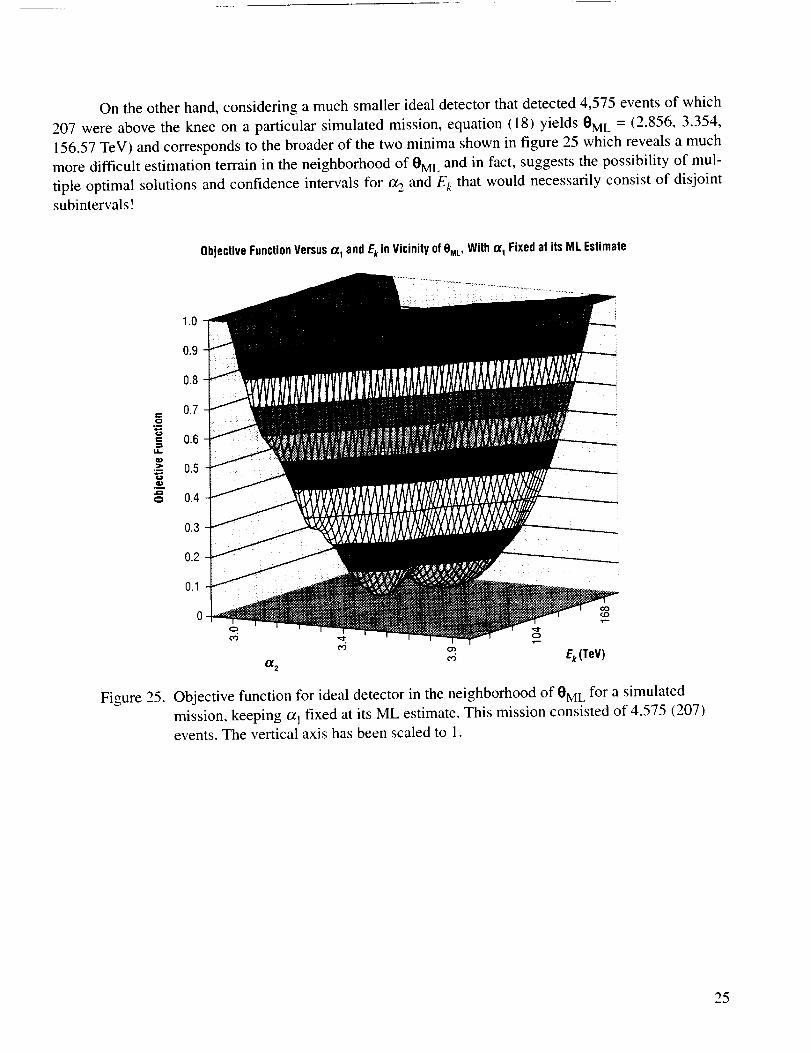
Ontheotherhand,consideringamuchsmalleridealdetectorthatdetected4,575eventsof which207 were abovethe kneeon a particularsimulatedmission,equation(18) yields 0ML = (2.856, 3.354,

156.57 TeV) and corresponds to the broader of the two minima shown in figure 25 which reveals a much

more difficult estimation terrain in the neighborhood of 0ML and in fact, suggests the possibility of mul-

tiple optimal solutions and confidence intervals for a 2 and E_: that would necessarily consist of disjoint

subintervals!

ObjectiveFunctionVersus O_1 and Ek in Vicinity of OML, With O_1 Fixedat its ML Estimate

o

e-

I,I.

g

0

Figure 25.

Ek(TeV)

Objective function for ideal detector in the neighborhood of 0ML for a simulated

mission, keeping a I fixed at its ML estimate. This mission consisted of 4,575 (207)

events. The vertical axis has been scaled to 1.

25

As observedin figures 13and 15,whenhistogramsof the ML estimatesof aj and c_, begin to

overlap, it clearly signals the onset of difficulties in estimating the broken power law spectral parameters

using MLE (and even more so for the method of moments since MLE was shown to be far superior in the

simple power law section of this TP). Thus, an important scientific question is, "For what values of E k willthese distributions likely begin to overlap for a particular detector?"

If the concept TSC with its 40-percent Gaussian response function is considered and with an

observing energy range of 20-5,500 TeV, then equation (20) provides the CRB for each of the three

spectral parameters as a function of E k. For example, for the case where 0 = (2.8, 3.3, E k) and calculating

the CRB for 75 _<E k < 400 TeV using equation (20), a 3_ curve describing the approximate width of the

distribution (histogram) of the ML estimate of _ as a function of E k can be constructed (3.3 minus three

times the CRB of _-,) for values of E k in the 75-400 TeV range. Sketching this curve versus E k and noting

where it begins to cross the line a I = 2.8 suggests the value of E/. where the lower 3_ point of the

distribution of the ML estimate of _2 for this concept TSC will likely begin to overlap that of a 1

(fig. 26(a)). Also shown in figure 26(a) is the case when the resolution is set to 20-percent and also zero-

percent (ideal detector), along with three addition dashed curves for the situation where the TSC's

collecting power is halved. Similar curves are provided in figure 26(b) for the case where a,_ = 3.1, giving

a spectral break size of 0.3. Obviously these figures are no substitute for statistical hypothesis testing and

furthermore do not consider the two errant estimation possibilities (EEl and EE2) that also suggest a

simple power law in favor of a broken power law, but nevertheless still provide important information.

3.3

ctz

3.1c_

I

2.9

2.750

(a)

Figure 26.

(ae- 3_cR8_Versus Ek for TSCand Half-Sized TSC • • •

a 2=3.3

_ "_o, .....

,* _'_'_'_. 0% (Ideal),/2o%

-.,t "_.'_._Z',, 40% (TSC

150 250 350

Knee Location - Ek (TeV)(0.5 Breaksize)

I

(b)

(a 2- 3_oRstVersus Ek for TSCand Half-Sized TSC • • •

iilIiiill.................,:::;................................ce 0% (deal)

I / 2o% I[ / 40 i?{rscfl29 .....: .......

50 150 250

Knee Location- Ek (TeV)(0.3 Bteaksize)

CRB used to estimate where the distribution of _x2 begins to cross that of a l

when (a) the spectral break size is 0.5 and (b) the spectral break size is 0.3.

26

Note, too, that thesefiguresrepresentabest-casescenarioin thatthey areconstructedusingtheCRB calculatedfrom equation(20) which of courseis not quite attainedin practice,especiallyfor thelargervaluesof E k and when the break-size is 0.3 as previously discussed. Thus, the actual overlap point

would occur sooner (that is, for smaller values of E k) because the variance of the ML estimator (or any

other unbiased estimator of a_) will be larger than the CRB.

Furthermore, figure 26 suggests that the 40-percent TSC is roughly equivalent to an ideal detector

of half its size in terms of measuring a2, while similar studies show this 40-percent TSC to be roughly

equal to a 20-percent resolution detector of half its size in terms of estimating _1 and Ek.2 Consequently,

instrument designers should consider first maximizing collecting power and then improving energy

resolution, whenever possible.

It is important to realize that while raising E 2 to higher values in this analysis offers no benefit for

this proposed TSC because of its previously stated collecting power, lowering E 1 does significantly benefit

the measurement precision of _1 and, because of their correlation but to a lesser degree, E k. However,

lowering E 1 offers no benefit in the measurement precision of _2_ when using the ideal detector and virtu-

ally none when using a real detector. These results are presented in table 4 for the case 0 = (2.8, 3.3, 100

Te;v') and in which E 1 is lowered incrementally from 20 to 1 TeV and once again illustrates the utility of the

CRB determined by equation (20). Results for the case when the break-size is reduced to 0.3 are similar.

Table 4. Effect of lowering E l on the CRB for the TSC-sized detector with 0-, 20-,

and 40-percent resolution Gaussian response function. The number

of events N 2 above E k is 2,255 for all values of E I.

E,

(TeV)

510152O

N

11,468,838632,364181,15286,98951,576

CRB-IdealDetector(O%)

_1 _2 Ek(TeV)

0.0005 0.0486 5.980.0024 0.0486 6.090.0050 0.0486 6.250.0081 0.0486 6.420.0117 0.0486 6.60

CRB-20%GaussianDetector

_X 1 5 2 Ek(TeV)0.0007 0.0578 7.890.0028 0.05791 8.160.0058 0.0581 8.560.0095 0.0584 9.030.0144 0.0586 9.58

CRB-40%GaussianDetector

_1 52 E,(TeV)0.0009 0.0691 9.920.0034 0.0697 10.490.0073 0.0704 11.340.0126 0.0713 12.35

0.0199 0.0722 13.56

1.4 Analysis of Multiple Independent Data Sets

The ML theory required to estimate spectral parameters from an arbitrary number of data sets

produced by science instruments having different observing ranges, different collecting powers, and differ-

ent energy response functions is developed in this section. Application of this methodology will facilitate

the interpretation of spectral information from existing data sets produced by astrophysics missions having

different instrument characteristics and thereby permit the derivation of superior spectral information based

on the combination of data sets. Furthermore, this procedure is of significant value to future astrophysics

missions consisting of two or more detectors by allowing instrument developers to optimize each detector's

design parameters through simulation studies in order to design and build complementary detectors that

will maximize the precision with which the science objectives may be obtained.

27

This extensionof themethodologydevelopedin theprevioussectionsto multiple datasetswasmotivatedby suchanapplicationandis presentedasanexamplein whichtwo detectors,bothassumedtohaveGaussianresponsefunctionsbut differentenergyresolutionsandobservingranges,weremodeledseparatelyandthenin acollaborativeeffort to estimatethesingleparameterof asimplepowerlawenergyspectrum.A succinctcomparisonof thebenefitsfrom usingthesetsin concertis measuredin termsofvariancereductionof theestimator,aswell asanybiasesresultingfrompoorstatisticsin oneor bothof theindividual datasetsthatmaybereducedwhenconsideredin combination.

TheML theorynecessaryfor applicationto multipleastrophysicsdatasetsis derivedherefor twoindependentdatasets,A andB, producedbyinstrumentshavingdifferent(1)observingranges,(2)collect-ing powers,(3) energyresponsefunctions,and(4) energyresolutions.Thesetwo datasetswill be usedtogetherto estimatetheenergyspectrainformationandtherebybenefitfrom thestrengthsof eachdetector,whereas,singly,theymaybeinadequatefor achievingthescienceobjectives.In practice,thedatasetsmustbecorrectedfor systematicerrorsin theenergyresponseof theinstrumentsin ordertoachievetheultimateaccuracyof thefinal spectrainformationbasedon thecombinationof astrophysicsdatasets.Generaliza-tion of thisapproachto morethantwo independentdatasetsthenfollowsby induction.

ToextendtheML theoryto handledatasetsA andB simultaneously,webeginwith theprobability

densityfunction for thedatasetof instrumentresponsesA = {x I ,x 2,.- ., XNA }, given by

gA(Xi ;0)= _ gA(XiIE.PA)(P(E;O)dE, i=L"-,N A ,

RA

so that the likelihood function is

(21)

NAI LA(0) = Ui=1

gA (xi I E, pA) _(E;O)dE] ,(22)

where 0 denotes the vector of spectral parameters of an arbitrary energy spectrum, _E;O), to be estimated;

N A is the number of detected events from observing range, RA, of instrument A having response function,gA, and energy resolution RA, so that the corresponding objective function is

O A(0) = -log [L A(0)] (23)

and the ML estimate e A, being that value of e for which OA(e) is a minimum, is obtained from equation(24) using the simplex search algorithm as

0 A = min O A (0) . (24)

28

Thelikelihoodfunctionandobjectivefunctionfor datasetB aresimilarly definedandbecausedatasetsA andB areassumedindependent,thelikelihoodfunctionfor thetwo setsconsideredsimultaneouslyis theproduct

LAB(0) = LA(0)LB(0) , (25)

so that upon taking the logarithm of each side gives the objective function as

OAB(0) = O A (0) + OB(0) (26)

and the vector of ML estimates based on both data sets considered simultaneously is

OAB----minOAB(O){o} = min{ol[OA(O) -b OB(O) ] .(27)

This procedure outlined above for two data sets is readily extended to k independent data sets so

that any one of the (2 k - 1) possible combinations of the data sets acting together provides the ML estimator

Os obtained by applying the Nelder-Mead algorithm to equation (28) as

0 s = mini _ Oj(O)

{o} lJ 6 S

(28)

where S can be any of the (2 k - 1) nonvoid subsets of the set of integers { 1, 2 ..... k }.

The statistical properties of the derived ML estimator can then be studied for each simulated

scenario and, in particular, those relating to (1) bias, (2) variance, and (3) normality can be rigorously

investigated using graphical procedures and appropriate statistical techniques. *'12"13

The CRB for the estimator of the vector of spectral parameters, O, using two independent data sets,

A and B, is derived in appendix B and shown to be the diagonal elements of the inverse of the covariance

matrix, I, whose 16 elements are

/_ log [gA(x;0)]16 (0) = N A_0 i

log [gA(X;O)]\ + NA/_ log [gB(Y;O)] ×

× _Oj / \ OOi

log [gB(Y;O)] /

30j /(29)

*Some statistical test procedures depend on the outcome of the normality test for estimators.

29

andwhere( 1)thenotation<. > denotes"expectedvalue"andin practicecanbeaccuratelycomputedusingGaussianquadratures;(2) thepartialderivativesarealsonumericallyevaluatedusingequation(15); and(3)gA(x;0) is the probability density function for data set A = {x i, i = 1..... NA}, given by equation (21 ) and

similarly for data set B = {Yi, J = 1..... NB}. As noted in appendix B, the CRB given by equation (29) is

readily extended to k independent data sets and provides a vital check on the performance of the derived

ML estimation procedure. If the simulations show the ML estimator of the spectral information to be

unbiased and also attains the CRB for a given spectrum-instrument combination, then this ML estimator

will be the best (minimum variance) unbiased estimator possible from combining multiple data sets for thatparticular astrophysics mission scenario.

Furthermore, when this ML procedure is used in the design phase of an instrument and if the

simulations show 0ML is unbiased and attains the CRB for the science mission under consideration, then

equation (29) can subsequently be used directly to evaluate the relative merits of various instrument design

parameters (measured in terms of their impact on reducing the statistical error in measuring 0) without

performing additional simulations. An example is given in section 1.6. This is of tremendous practical

benefit because equation (29) can be evaluated in mere seconds while the equivalent information based on

Monte Carlo simulations can take several days to obtain. Extending the ML procedure to multiple data

sets, where in practice each may contain 105 to 106 events for a given science mission, is quite challenging.Practical studies conducted in Howell1.2 typically required >1,000 simulated missions to obtain statisti-

cally meaningful inferences about a single detector design parameter under study. Such a simulation run

would last >12 h when the broken power law spectrum was assumed (considerably less for the simple

power law), largely because of the vast number of numerical integrations required in evaluating the

objective functions and the many steps taken by the Nelder-Mead search for 0ML.

1.5 Example of Estimating ¢_1 of a Simple Power Law Using Two Data Sets

The benefits of having the additional nuclei (Z > 8) from a proposed thin sampling calorimeter

(TSC) for ACCESS at energies above the transition radiation detector (TRD) energy range was recently

investigated 14 using this methodology and serves to illustrate the application and utility of the approach.

Specifically, the value of having these calorimeter-provided nuclei in addition to the expected number of

TRD events was investigated, and the approach was to measure the benefit of including these additional

events in the estimation of the single parameter, O_1, of an assumed simple power law as compared to notincluding them.

In this example the TRD geometry factor is assumed to be 7.58 m2-sr with energy response saturat-

ing at 20 TeV/n and for an observing period of 1,000 d. Furthermore, it was decided to consider the species

Ne-S with an assumed differential spectral index of 2.39, along with a calorimeter geometry factor of

5 m2-sr, providing 593 events >20 TeV/n on average for the calorimeter for a 1,000-d observing period.

Additionally, a Gaussian response function was assumed for both detectors, and the TRD was

assumed to have the same linear mean response as the calorimeter but with a constant 35-percent energy

resolution over its observing range E 1 to 20 TeV/n, while the TSC was assumed to have a constant resolu-

tion of 40-percent over its nonoverlapping observing range 20 to 2,000 TeV/n. This upper limit of 2,000

TeV was chosen for the calorimeter because the number of detected events >2,000 TeV is negligible for a

detector of this collecting power. Then, E l is taken to be different values ranging from 0.5 to 7 TeV as part

3O

of a parametric study in this illustration. Of course, the upper energy boundary of 20 TeV/n could be

extended to a higher value if the saturation limit of the TRD could be improved.

In the simulation, GCR event energies, E i, are simulated from the TRD observing range, RTR D

= [E l, 20 TeV], and where the number of these events, NTR D, is a function of the observing range, geom-

etry factor, and observing time. Then, for each of these simulated incident energies, E i, a response, x i, is

simulated according to the assumed Gaussian response function and with 35-percent energy resolution,

PTRD" The calorimeter events are simulated in a similar manner using its defining parameters, NCa 1, Rca 1,

and PCal, and the Gaussian response function.

Performing the simulation once defines a so-called astrophysics "mission" and provides a single

ML estimate of _z1for each instrument by solving equation (24) with 0 = a 1 and all instrument characteris-

tics appropriately modeled through the formulation of the detector response function, g, for each detector,

and then solving equation (27) when the two data sets are used in combination in the ML estimation

procedure. Notationally, O_Ca1and _rRD are the ML estimates of oq when the calorimeter and TRD are

considered as standalone instruments, respectively, and OeBoth is the ML estimate of a I when the two

instruments are used in combination. The simulation is repeated for many missions, each time generating

a new set of incident energies from the assumed simple power law spectrum for each instrument and their

respective simulated energy deposits according to the detectors' response functions, estimating a I using

each data set separately and then in tandem. The statistical behavior of these estimates relative to plausible

design variation of response function parameters is then studied.

Figure 27a shows the ML estimates C_q-RD, aCa 1, and aBoth of a I for 25 simulated missions in which

E l was first set to 5 TeV/n, thus providing 5,275 events on average for the TRD. Figure 27b shows the

effect of lowering E l to 3 TeV/n, providing an average 11,660 events for the TRD, and then lowering E 1 to

1 TeV/n, providing an average of 56,920 events for the TRD for 25 missions (fig. 27c). We observe that as

E l is lowered, thereby increasing the number of TRD events as well as extending its effective observing

range, and hence "lever arm" effect in the estimation of a I, the calorimeter has an ever-diminishing role in

its contribution to O_Both as illustrated by the I_-RD and aBoth estimates nearly coinciding in figure 27c.

E

¢,#1

,...I

Oq,-R D + O_Both _ Or,Ca I

2.6

2.5

2.4

2.3

2.2

........... ..................... ...... !, ..............

'm:/'W III ",'U"

........... -- : ...... ,_--_-- ,',.... '_- .................. a- -_-_, .... ;_"

i i i i

0 5 10 15 20 25

Mission

Figure 27a. ML estimates of a I for 25 missions, with E l = 5 TeV (5,275 events for TRD

and 593 for calorimeter).

31

C_rR D _ (ZBoth "''"Am O_caI

2"6 t A

2.5 .............................................. ._ ...............,I_ ,A

2.3 Jr ........... .......... _--_ ........................ _- ........ . .__

2.2 /

0 10 15 2O 25Minion

Figure 27b. ML estimates of a I for 25 missions, with E l = 3 TeV ( 11,660 events for TRD

and 593 for calorimeter).

UqRD _ _8oth _ _Cal

2.6

2.5

2.4

2.3

2.2

A

hit A ,t, A

A A _

....................... ,__,_........................ _ ......... ;(A

0 5 10 15 20 25

Mission

Figure 27c. ML estimates of a] for 25 missions, with E t = 1 TeV (56,920 events for TRD

and 593 for calorimeter). Note that tZrR D and aBoth are virtually indistinguishable.

32

The simulation was run for 1,000 missions for each of several values of the E 1 parameter with

summary statistics provided in table 5 for the calorimeter acting alone; table 6 for the TRD acting alone;

and table 7 for the two data sets acting in concert to estimate tz 1 . Tables 5 and 6 show that the calorimeter

and TRD as standalone instruments each provide unbiased spectral information (recall cz] = 2.39 for this

study) and attainment of the CRB.

Table 5. Summary statistics of O_CaI based on 1,000 simulated missions of the calorimeter.

Calorimeter Standard

E1 (TeV) E2(Tev) EventsN(E> El) Mean Deviation_cal CRB20 2000 593 2.39 0.066a 0.067a

aTheappearancethat(_calis lessthanthe CRBis anartifactof thefinitenumberof missionsinthesimulations.

Table 6. Summary statistics of C61-RD based on 1,000 simulated missions for each value

of E 1 of the TRD alone (all events between E L and 20 TeV).

E, (TeV)

7

5.2

5

3

1

0.5

Saturation

(TeV) TRD Events

20 2968

20 4947

20 5274

20 11,658

20 56,919

150,6302O

Mean

2.39

2.39

2.39

2.39

2.39

2.39

Standard

Deviation(_TeO CRB

0.124 0.123

0.068 0.068

0.063 0.063

0.031 0.031

0.011 0.011

0.007 0.007

Table 7. Summary statistics of aBoth based on 1,000 simulated missions for each value

of E 1 of the TRD and calorimeter acting in combination.

CRBfor TRD andCalorimeter (Includes593 Events>20 TeV)

TRD

Saturalion

E, (TeV) (TeV)7.0 20

5.2 20

5.0 20

3.0 20

1.0 2O

0.5 20

Calorimeter

(TeV) E_(XeV)20 2,000

20 2,000

20 2,000

20 2,000

20 2,000

20 2,000

Total Combined Standard

Events Mean DeviationO_th CRB

3,560 2.39 0.058 a 0.059

5,539 2.39 0.048 0.048

5,866 2.39 0.045a 0.046

12,249 2.39 0.027a 0.028

57,511 2.39 0.011 0.011

151,220 2.39 0.007 0.007

Theappearancethat(_calis slightlylessthantheCRBis anartifactof thefinitein thesimulations.

numberof missions

33

Table 7 shows that for all scenarios considered, the two data sets acting together likewise provide

an unbiased estimate of the spectral parameter, al, and attainment of the CRB computed from

equation (29) with 0= a I to give

as the CRB for the TRD and calorimeter acting in combination. The CRB in table 5 corresponding to the

calorimeter acting alone is obtained from equation (14) and likewise for the TRD acting alone. Numerical

evaluation of equation (30) for the different scenarios of interest presented in table 7 indicates the two

detectors acting in concert do indeed attain the CRB for all values of E I. Achievement of this bound,

coupled with the fact that the derived ML procedure provides an unbiased estimate of the spectral param-

eter, a I, implies that this procedure is the best (minimum variance) unbiased estimation techniquepossible.

Additionally, histograms of the 1,000-mission ML estimates for each instrument considered

separately and also in tandem show the distribution of the ML estimator to be approximately normallydistributed.

Comparing standard deviations of the different scenarios in tables 5-7 clearly shows the impor-

tance of not only the number of events or so-called "statistics" but also the observing range of the instru-

ments: i.e., the "'lever arm effect." The very special case where E 1 = 5.2 TeV, found by trial and error, shows

the calorimeter acting alone with only 593 events but with a much greater observing range (20 TeV/n to an

average maximum event energy of 1,100 TeV/n) is effectively as good as the TRD in terms of estimating

t_ 1 (CYcaI = 0.067, and _TRD = 0.068 when E I = 5.2 TeV). For this case where E I = 5.2 TeV, the TRD had an

average of 4,947 events but with a much shorter observing range. Furthermore, the TRD's energy resolu-

tion was assumed to be 35 percent, whereas the calorimeter was assumed to be worse with a constant

40-percent energy resolution. We also note the fairly intuitive result in table 7 that C_Both= 0.048 which is

-_0.068/_2 when the calorimeter and TRD are effectively equal to each other and so O'Both scales roughlyby _2 for this case.

Nevertheless, as E 1 is successively lowered, we note the overpowering impact of the TRD's

increasing number of events and growing observing range, and in fact, for E l < I TeV, the calorimeter's

contribution to the variance reduction of the ML estimate of 6_Both is virtually nil. Thus, we see that "how

low" the TRD can observe plays a major role in assessing the value of these additional calorimeter events

in the estimation of the spectral parameter, a 1. It was concluded that since the proposed TRD would easily

observe to <1 TeV/n, the contribution of the calorimeter's additional events would be insignificant for

measuring the spectra for Z > 8. Thus, this study resulted in an important design consideration for the

charge particle identification detector for the calorimeter and underscores the utility of this ML theory for

multiple independent data sets in the design phase of new science instruments.

34

1.6 Using the CRB to Explore Instrument Design Parameters When Estimating

0 = (or1, 0.2, E k) of a Broken Power Law Using Three Data Sets

The benefit of using three independent data sets in concert to measure the spectral parameters of an

assumed broken power law proton spectrum will be investigated, and, for specificity, assume the spectral

knee location is E k = 175 TeV and the slope parameters al/_7.2_ below/above the knee are 2.8 and 3.2,

respectively, to give a 0.4 spectral break-size.

Next, assume the three hypothetical data sets A, B, and C were collected by instruments having

observing ranges, collecting powers, and stochastic response functions defined in table 8 so that data set A

provides information regarding only the spectral parameter a I; B about a I, c_2, and Ek; and C, only about

_,. It is further assumed that each data set was produced by a detector having the same linear mean

response as the TSC previously introduced in section 1.1 so that their response functions may be visually

compared in figure 28.

Table 8. Data sets and associated response functions, with CRB for all possible

combinations of data sets.

DataSetCombinationsandInstrumentResponseFunction

ObservingAverageNumber

Range(TeV) ofEvents

A (Gaussian) [1,20] 150,000B(Gamma) [35,5,000] 44,000(2,000)*

C (BrokenGaussian) [500,10,000] 500AB

Cramer-RaoBoundfor

BCABC

*44,000eventsabove35TeVof which2,000areaboveEk=175TeV.

_1 % Ek(XeV)0.0095 - -0.0225 0.0780 34.24

- 0.1050 -

0.0087 0.0744 26.130.0220 0.0626 30.230.0087 0.0607 23.05

In this scenario, data set A was produced by an instrument having a Gaussian response function and

with constant 40-percent energy resolution; B by an instrument having a gamma response function and

thus capable of describing a wide variety of shapes with right-hand skewness (outer curve from the right in

fig. 28); and C was measured by a detector having a "broken Gaussian" response function consisting of

two blended normal distributions (middle curve from fight in fig. 28) suggested by J. Ormes, 2000, private

communication, for its closeness to the Gaussian response function but with a tail region as desired. These

latter two response functions were introduced to address the possibility that some detector response func-

tions may exhibit a fight-hand skewness and might add to the difficulty of the ML estimation task. Note

that while the gamma response function used here also has a constant energy resolution of 40 percent, the

broken Gaussian actually has a 4 l-percent resolution because of the added skewness while keeping the rest

of the distribution matching the Gaussian.

Furthermore, in the construction of these hypothetical data sets, the number of events in each data

set was chosen so that each data set alone provides unbiased spectra information and approximate

attainment of the CRB, I,2 as discussed in sections 1.1 and 1.2, so that any combination of the data sets

35

.... BrokenGaussian _ Gaussian -- Gamma

0.009

0.006 ............................................................

_- 0.003 ..........

o ,0 100 200 300 400

EnergyDeposit(GeV)

Figure 28. Gamma, Gaussian, and broken Gaussian detector response functions to 40-TeV proton.

should also attain the CRB. Consequently, the CRB can be calculated from equation (56) for the

combination of data sets and used directly to investigate the relative merits of instrument design parameters

without performing the simulations. Note that while A and C provide no information about the knee loca-

tion E k, they do provide an improvement in the measurement precision of E L.when they work together withdata set B.

To illustrate the utility of the CRB for multiple independent data sets regarding design parameter

studies, suppose the collecting power of instrument C is increased by a factor of 10 with the results given

in table 9 which shows the merits of collecting power on the measurement precision of the spectral param-

eters for the combinations of data sets C, BC, and ABC. While C only contains information about __, the

measurement precision (standard deviation) of E k reduces from 30.23 to 23.6 TeV for the BC combinationand from 23.05 to 17.47 TeV for the ABC combination.

Table 9. Number of events from table 8 in data set C ]s increased by a factor of 10.

InstrumentCombinationObserving

Range (TeV)

AverageNumber

of Events

A (Gaussian) [1,20] 150,000

B (Gamma) [35, 5,000] 44,000 (2,000)*

C (Broken Gaussian) [500, 10,000] 5,000AB

BC

ABC

"44.000eventsabove35 l'eVof which2,000areabov E_=175TeV.

Cramer-RaoBoundfor

0.0095

0.0225

0.0087

0.0214

0.0086

% Ek (XeV)

0.0780 34.24

0.0332

0.0744 26.13

0.0306 23.60

0.0303 17.47

36

Next, if the number of events in data set B is reduced by a factor of 2 and those in C increased by a

factor of 10, we can once again explore the impact of various collecting power options shown in table 10.

Finally, if we keep the collecting powers the same (B reduced by a factor of 2, C increased by a factor of

10), and additionally improve the resolution of the instruments for A and C to 30- and 35-percent

resolution, respectively, we see the impact of detector energy resolution on measurement precision of the

spectral parameters, as shown in table 11.

Table 10. Number of events from table 8 in data set B is reduced by a factor

of 2 and those in C increased by a factor of 10.

InstrumentCombinationObserving

Range(TeV)

AverageNumberof Events

A (Gaussian) [1, 20] 150,000

B (Gamma) [35, 5,000] 22,000 (1,000)*

C (Broken Gaussian) [500, 10,000] 5,000

A8

BC

ABC

*22,000eventsabove35TeVof which2,000areaboveEk=175 TeV.

Cramer-RaoBoundfor_1 % E, (XeV)

0.0095 - -

0.0318 0.1104 48.42

- 0.0332 -

0.0091 0.1048 35.86

0.0302 0.0318 31.81

0.0090 0.0317 22.36

Table 11. Number of events from table 8 in data set B is reduced by a factor

of 2 and those in C increased by a factor of 10, resolution of A improved

to 30 percent and C to 35 percent.

ObservingRange (TeV)

B (Gamma, 40%)

AverageNumberof Events

Cramer-RaoBoundlor

InstrumentCombination _1

A (Gaussian,30%) [1, 20] 150,000 0.0083

[35, 5,000] 22,000 (1,000)* 0.0318

[500,10,000] 5,000 -0.0080

0.0301

0.0080

C (BrokenGaussian,35%)AB

BC

ABC

*22,000eventsabove35TeVof which2,000areaboveEk=175TeV.

% E, (TeV)

0.1104 48.42

0.0321

0.1047 35.58

0.0309 31.70

0.0307 22.02

Obviously, the number of possible parametric studies are numerous, but the preceding sample

investigation illustrates the utility of this procedure and the derived CRB for multiple independent data sets

when considering the design of new, complementary detectors. Furthermore, the CRB in tables 8-11 were

computed using equation (56) in <1 min, whereas the equivalent information based on Monte Carlo simu-

lations would take > 1 week to obtain. However, when the CRB is not attained in practice, simulations must

be used to estimate the real performance benefits when using multiple independent data sets.

37

2. CONCLUSIONS

This TP investigates the statistical properties of the ML estimator of the single parameter of a

simple power law energy spectrum and presents the conditions under which this estimator attains the three

desirable properties: (PI) consistency, (P2) efficiency, and (P3) asymptotic normality. A comparison with

the estimation procedure called the method of moments is also included and shows the ML estimator to be

far superior in terms of these three desirable properties.

The properties of the ML estimator of the broken power law energy spectral parameters and the

conditions under which P l, P2, and P3 are attained are also investigated under a wide range of parametric

values. A crucial result of this research and necessity for investigating P2 is the derivation of a closed-form

expression for the CRB of the broken power law distribution presented in appendix A. Another critical

result is the calculation of the CRB using equation (20) for the broken power law distribution and equation

(14) for the simple power law distribution when events are measured by a real detector having response

function, g, and energy resolution, p. While this study considered an instrument having a Gaussian re-

sponse function and with resolutions ranging from zero to 50 percent, any response function, g, can be used

in equations (14) and (20) to calculate the CRB, such as various skewed distributions and others having

nonconstant energy resolution as illustrated in section 1.6 and also discussed in references ! and 2. Much

insight into the estimation task of power law spectra information can be gleaned from the CRB as illus-

trated in this TP, as well as the fact that it provides a stopping rule in the search for the best (minimum

variance) unbiased estimator of power law spectra information.

Simulations were conducted in parallel with these analytical results and the CRB played an unex-

pected but valuable oversight role by signaling errors in the simulation code when the simulations occa-

sionally produced the impossible result of the ML estimator having a standard deviation smaller than the

CRB. Furthermore, it is likely that these simulation errors, while small in practical terms, would have gone

unnoticed if not for having the CRB available for comparison.

Additionally, several detector design parameter studies are included in this research and it is hoped

that those designing instruments to measure power law spectra information will benefit from these studies.

Additionally, this analysis should benefit those wishing to apply these techniques to the estimation of

spectra information from existing data sets, which requires a modified likelihood function to handle the

realistic situation in which the range of integration [El, E2] in the objective function is unknown, and isdiscussed in detail with examples in references 1 and 2.

The MLE procedure and companion analytical techniques to estimate spectra information from an

arbitrary number of astrophysics data sets produced by vastly different science instruments is presented

and demonstrates how complementary astrophysics missions can work in concert to achieve science goals.

Additionally, the CRB for an unbiased estimator of spectra information based on these multiple indepen-

dent data sets is derived in appendix B and provides a means of assessing the accuracy of different estima-

tion techniques and, furthermore, provides a stopping rule in the search for estimation methodologies

when the CRB is attained in practice. Several examples illustrating this ML method and utility of the CRBfor multiple independent data sets are included.

38

APPENDIX A--CLOSED-FORM EXPRESSION FOR THE CRAMER-RAO BOUND

OF THE BROKEN POWER LAW

A closed-form expression for the information matrix I(0) of the broken power law distribution is

derived, and the inverse I-l(0) is defined as the CRB. This bound corresponds to the so-called ideal

cosmic-ray detector having perfect energy resolution and has tremendous utility because it sets the limit on

the precision with which any conceivable detector of equal collecting power can measure the three broken

power law spectral paramaters. Furthermore, it provides a means to tune the integration and differentiation

parameters in the numerical algorithm for evaluating equation (20) for real detectors because the CRB

determined from equation (42) is exact and must equal equation (20) when the detector's energy resolution

9-->0.

A.I Derivation

The broken power law probability density function for GCR event energy, E, is given by

OB (E;O) =

A(0)f E] -¢zl for

kE )( E

A(O)[--_k ) for

E l < E < E k

E k <_E < E 2

(31)

over an energy range [E l, E 2] that does not depend on the spectral parameters 0 = (a 1, _z2, Ek), and the

normalizing coefficient A(0) is:

A(0) =(a I - 1)(o: 2 - 1) (32)

r ", l-a_ J

. _l)[E_,/ -E k al - 0_'_+ (av - 1)[ El / -(a l_ _ !,,Ek) _Ek)

Starting with

IX

E3

_ C_B( E;OktE

E_

Ek

I elog[Oe_E:OlldE +

El

E_

I elog[OB(E:O)]dE

Ek

(33)

39

and writing log[(PB(E: 0)] as

where _i and _2 are indicator functions defined in equation (37), gives

(34)

E, L _k J L Ek J"

+ f_ exp log[A(0)]-a Iiog 61 -a llog 62 dE

El . L

Taking the derivative of equation (35) with respect to _1 and a, is straightforward and gives

(35)

o=\(36)

where <. > denotes mathematical expectation and the abbreviations

A'I- _ 'A2- _ 'LE--I°g tz/.j O'E>E k 1. E> E_(37)

are introduced. Taking the derivative of equation (35) with respect to E k and using Leibnitz's rule (seeProfessor Bierens" "check" of equation (39) in section A.2):

qa dq

P 1'

and the continuity of Ot_ at E/. gives

(38)

40

0_E_ 01og[cPB(E;0)]_ (_. OE k feB E;O)dE +OB(Ek;O)-O+

El

E2

OI°g[OB(E;O)]OB(E;O)dE + O- OB(Ek;0)3E k

Ek

whereand the three partial derivatives of log[A(e)] defined in equations (37) and (39) are

(39)

AI=t,_) E, E_+¢-I+,_,)E_- _Ek) LkJ)

(-l+_l) -z__ _Ek)a_, = (40)

- - _,_tJ _,ek) (- - -_,ek)

_,Ek ) [ (-1 + cq)°_2E2 + (-°q + °_2) Et

As a check, the expectation of the partial derivatives of OB with respect to the parameters 0f 1, ,G62,

and E t defined in equations (36) and (39) are indeed seen to be zero when the derivatives A 1, A 2, and A t in

equation (40) are used in conjunction with the expected value terms defined in equation (41), along with

(61) = Pr{ E < E k }, and (62) = 1- Pr{ E < E k }, and

41

4-I..;, A A

_t"T.' r",+ pl..j i J

v v

II II

i q

I...I

_I,+_

, +

I LuI.._ I

I +

+

° i__• +

l--J

I I

T ++ __

IJ

IJ 0

IJ

t_

p.o

g

e_

_°©

a"

f_

0

I,.._

©

<_°

©

,<

<

e_

v

L,,.+ _+,_ I J '.,,,,1 l J --

II II II II II II

II II II

+

:.,.+ ::+..- ,_. +_

+ + +

,+ - _ _,_ +

i

2..,- _ ''" ",.+'- _ __ +

_ I l-.J___,_ _,_,_ _• _ _ -

t'h

_ v ___ +

_ - _,_ 1-_

i,., I -- +

I I

'-_ II

_o -_-

+

A

_ v

B

O,.,-h+ I

_ +

_-_ ,+

_ +

_" r--I

_ _._I,_

an¢'3 I_

_ ,

©

,o

A

v

III

I

I

+

+

w

0

I--1

i iI

©0_

r--1

1 1

Finally, the matrix elements defined in equation (42) are multiplied by N to give the information

matrix I(0). It is interesting to note that I(0) contains the intuitive terms N<fil> and N<62>, which are the

expected number of events below and above the spectrical knee E k, respectively.

This completes the derivation of the closed-form expression of the information matrix I(0) corre-

sponding to the so-called ideal detector having perfect energy resolution. Its inverse I -I (0) gives the CRB,

and the square root of the diagonal elements of 1-1(0) is the CRB for the three spectral parameters. In

practice, one should verify that the difference of the covariance matrix C and the CRB is positive definite

by checking that the eigenvalues of the matrix [C- I-1(0)] are all positive. If the eigenvalues are zero, the

CRB has been reached and the ML estimator has attained property P2 (efficiency) by achieving the CRB.

The computer program MATHEMATICA 15 was used to provide equations (40)-(43) and performed

the important check

(44)

that confirms the correctness of the terms leading to the construction of the information matrix l(O). Fur-

thermore, a format feature of MATHEMATICA called FortranForm was used to write these equations in

FORTRAN source code for implementation in the overall simulation program and thereby eliminated the

possibility of introducing human error in transferring the equations into the computer program.

A.2 Check on Equation (39) by Professor Bierens 16

"Equation (39) is correct if (38) is correct, which in its turn is the case if (38) holds for fixed p and

q. In the latter case (38) states that the derivative operator d/da can be moved inside the integral, which

requires the application of the dominated convergence theorem. The conditions for the latter are:

1. For each x in [p,q], f(x,a) is differentiable in a, possibly except for x in a subset with Lebesgue

measure zero.

2. There exists a function b(x,a), say, with finite integral over Lo,q] such that sup{n[f(x,a+l/n)-f(x,a)]

< b(x,a) and sup{ n[f(x,a-1/n) -f(x,a)l < b(x,a), where the "sup" is taken over all 17>0.

In (39) you have applied (38) for the cases q = a and p fixed, and q fixed and p = a, so that (39) is

correct if the conditions 1 and 2 hold for a = q and a = p. In the case q = a and p fixed, the log-densityf(x,q)

is differentiable in q for x < q, but not for x = q. Similarly, in the case q fixed and p = a,flx,p) is differen-

tiable in p for x > p but not for x = p. Thus condition 1 holds, with {p,q } the subset with Lebesgue measure

zero. Moreover, since the left and right partial derivatives off(x,a) to "a" are bounded, condition 2 holds as

well. Consequently, (39) is correct?'

43

APPENDIX BmCRAMER-RAO BOUND FOR MULTIPLE INDEPENDENT DATA SETS

Derivation of the CRB using two independent data sets, A and B, considered simultaneously to

estimate a single spectral parameter, 0, follow along the lines of the proof of the CR inequality in Hogg and

Craig 17 for a single data set. Starting with the probability density function for detector A's response (e.g.,

energy deposit)data set A = {x i i= 1,...,NA } as

gA(xi;O)= I gA(xi ]E'PA)(P(E;O)dE' i= 1,-..,N A

R A

(45)

and similarly for data set B= {yj] j= 1,-.-,NB} as

gB(Yj ;0)= f gB(Yj [E,PB) q_(E; O)dE, j = 1,..., N B ,

RB

(46)

and because

1= f gA(Xi;O)dxi, i= I,...N A

R A

(47)

and also for data set B, their product gives the joint probability density function of the two data sets

considered simultaneously. Assuming the derivative operator d/dO can be moved inside the integral,

differentiating their product with respect to 0 gives

[. 03log [ga(xi;O)]0J 030

R A

Next, define the random variable, Z, as

[ 03 log [gB(yj;O)]gA (Xi;O)dxi +030 gB (Yj; 0 )dyjd

R B

(48)

N2_..,A_-, 03log [gA(xi;O)] 03log [g_(yj;O)]

Z030 + c)0

i=1 j=l

_49)

44

It follows from equation(48) that the meanof Z is zero, or using expected value notation, <Z> = 0.

Moreover, Z is the sum of (N A + N B) mutually stochastically independent random variables, each with

mean zero and consequently with variance*

{) log [g,(x;O)] 2 _ log y;0)] -

°'z = NA D0 + Nr_(50)

Next, assume there exists an unbiased statistic, U, of the parameter 0 that is a function of the (N A + N B)

instrument responses comprising data sets A and B considered acting together, so that

U = U(Xl,..., XNA, Yl, "", YN B ) and hence

f "" _ ll(XI,'" ", XN A ,3'1'" "' YN B )ga(Xl ;q)"" gA(XNA ;q)gS(Yl ;q)

R B RA

• "gB(YNB ;0)act" 1, "", dXNA, dYl,-", dYNB

(51)

and differentiating both sides with respect to 0 gives

R B R A g A ( Xi ; q )

OgA (xi;q)

Oq

+ E 1 Ogtl(3_/;q) × gA(Xl;O)...gA(XN a;O)gB(yl;O)

j=l gB(Yj;q) Oq

• .. gB(YNB ;0)drl ""drNAdyl ""dYNB

, [ Na 3log[gA(xi;q) ]

= _'"_u(xI'""XNa'YI''"'YNs)[i_=I OqR8 RA

+ NBE 0 log [gB<YJ;q)] ]×0q gA(Xl;O)'"gA(XNa ;O)gB(Y';O)

j=l J

•..,,(.vN. d.,-N +N. (52)

*The expectation of the cross-product terms is zero because of independence.

45

Thisshowsthat<UZ> = 1,and,because<UZ> = <U><Z>+ r _u°'z,wherezis the correlation coefficientof U and Z, we have

Il=O×O+r_YuCr Z or r=--- (53)

CYUGZ

Since r 2 < 1, it follows that ¢Yt7I> 1/¢Yz and therefore

o'/_

r0 log (x:0)] 0 log [gB (y;0)]'_

NA , +NB _ ) /

which establishes the CRB for two independent data sets, A and B, for an unbiased estimator of the single

spectral parameter of an energy spectrum. This bound readily extends to k independent data sets by induc-

tion and furthermore confirms that "it always pays to use additional data sets" because of the additional

v_u'iance reduction and hence improvements in measurement precision, as long as the additional data setsprovide unbiased information.

The above derivation generalizes to the case where 0 is a vector of spectral parameters by the

additivity of information matrices 18 so that the CRB for the individual parameters comprising 0are the

diagonal elements of the inverse of the information matrix, I, having/j-elements

NA/_ log [gA(X;0)] _ log [gA(X;0)]\16 \ + NB(O log Ooi[gB(y;0)] _ log _j[gB(Y;0)]\/ (551

and, as in the single parameter case, equation (55) is readily extended to k independent data sets.

46

For the interesting case where a detector does not observe events in an energy range represented by

one or more of the spectral parameters, the partial derivatives with respect to those parameters are zero. For

example, suppose detector A observes only events below the spectral knee, detector C only observes events

above the knee, and detector B observes both above and below the knee. Then the matrix to be inverted to

obtain the CRB for an unbiased estimator of 0 = (a t, _, E k) is

0 log [gA(X;al )] 0 0

lij=N A 0 0 0

0 0 0

(3 log [g_ (y;0)] _ log [gs (y;0)] /+NB O0 i _ /

+N C

-0 0

o0 0

_

0 ,

0

(56)

where the notation in the second term of the right-hand side of equation (56) defines 01 - _1, 02 = a2, and

03 --E k as before and where the inte_ation range for this term must be split at E k in its numerical evaluation.

An example us;-,,- ,_auation (56) is provided in section 1.6 of this TE

47

REFERENCES

J° Howell, L.W.: "Maximum Likelihood Estimation of the Broken Power Law Spectral Parameters With

Detector Design Applications," Nuclear h_struments and Methods in Physics Research Section A:

Accelerators, Spectrometers, Detectors and Associated Equipment, In Press.

. Howell, L.W.: "A Recommended Procedure for Estimating the Cosmic-Ray Spectral Parameter

of a Simple Power Law," Nuclear Instruments and Methods in Physics Research, Vol. 480(2-3),

pp. 739-751.

3. Kendall, M.G.; and Stuart, A.: The Advanced Theo_' of Statistics, Vol. 2, 2nd ed., Hafner Publishing

Company, New York, NY, pp. 8-10 and pp. 35-67, 1963.

4. Press, W.H.; et al.: Numerical Recipes in FORTRAN, Cambridge University Press, New York, NY,

pp. 402-405, 1992.

5. Press, W.H.; et al." Numerical Recipes in FORTRAN, Cambridge University Press, New York, NY,pp. 140-155, 1992.

6. Kendall, M.G.; and Stuart, A.: The Advanced Theoly of Statistics, Vol. 2, 2rid ed., Hafner Publishing

Company, New York, NY, pp. 8-10 and pp. 55-60, 1963.

7. Bierens, H.J." Topics in Advanced Econometrics, Cambridge University Press, New York, NY,

pp. 60-67, 1994.

8. Lehmann, E.L.: Theoo, of Point Estimation, John Wiley & Sons, New York, NY, pp. 409-443, 1983.

9. Voinov, G.G.; and Nikulin, M.S.: Unbiased Estimators and Their Applications, Kluwer Academic

Publishers, Dordrecht, The Netherlands, pp. 90-104, 1993.

10. Lee, J.; Watts, J.; and Howell, L.: "Simulations of a Thin Sampling Calorimeter with GEANT/FLUKA,"

Nuclear Instruments and Methods in Physics Research, Vol. 470, pp. 500-511,2001.

!1. Press, W.H.; et al.: Numerical Recipes in FORTRAN, Cambridge University Press, New York, NY,pp. 180-181, 1992.

12. Brownlee, K.A.: Statistical Theor). , and Methodology in Science and Engineering, John Wiley & Sons,Inc., New York, NY, 1960.

13. Conover, W.J.; Johnson, M.E.; and Johnson, M.M.: Technometrics, Vol. 23(4), p. 351, 1981.

48

14. Proceedingsof the ACCESSCollaborationMeeting, J.H. Adams,ed., National SpaceScienceTechnologyCenter,Huntsville,AL, January17-20,2001.

15. Wolfram,S.:MATHEMATICA, Version 4, Wolfram Research, 1999.

16. Bierens, H.J.: Department of Economics, The Pennsylvania State University, University Park, PA,

Private Communication, 2001.

17. Hogg, R.V.; and Craig, A.T.: bztroduction to Mathematical Statistics, 3d ed., The Macmillan

Company, New York, NY, 1972.

18. Lehmann, E.L.: Theom of PohTt Estimation, John Wiley & Sons, New York, NY, 1983.

49

REPORT DOCUMENTATION PAGE Form Approved

OMB No. 0704-0188

Public repor_r_l burden for this collection of information is estimated to average 1 hour J;)erresponse, including the time for reviewing instruchons,searching existing data sources,gathenng and maintaining the dala needed, and completing and reviewing the collection of information Send comments regarding this burden estimate or any other aspect of thiscollection oi reformation, incluaing suggestions for reducing this burden, to Washington Headquarlers Services, Directorate for Inlormation Operation and Reports, 1215 JeffersonDavis Highway. Suite 1204, Arlington, VA 22202-4302, and to the Office of Management and BudgeL Paperwork Reduclion Prolect (0704-0188)1 Washington. DC 20503

1. AGENCY USE ONLY (Leave Blank) 2, REPORT DATE 3. REPORT TYPE AND DATES COVERED

September 2002 Technical Publication4. TITLE AND SUBTITLE 5. FUNDING NUMBERS

Statistical Properties of Maximum Likelihood Estimators

of Power Law Spectra Information

6. AUTHORS

L.W. Howell

7. PERFORMINGORGANIZATIONNAMES(S)ANDADDRESS(ES)

George C. Marshall Space Flight Center

Marshall Space Flight Center, AL 35812

9. SPONSORING/MONITORINGAGENCYNAME(S)ANDADDRESS(ES)

National Aeronautics and Space Administration

Washington. DC 20546-0001

8. PERFORMING ORGANIZATION

REPORT NUMBER

M-1056

10. SPONSORING/MONITORING

AGENCY REPORT NUMBER

NASA/TP--2002-212020

11, SUPPLEMENTARY NOTES

Prepared by Space Science Department, Science Directorate

12a. DISTRIBUTION/AVAILABILITY STATEMENT

Unclassified-Unlimited

Subject Category 90Standard Distribution

12b. DISTRIBUTION CODE

13. ABSTRACT (Maximum 200 words)

A simple power law model consisting ola single spectral index, ct, is believed to be an adequate description ol the galactic cosmic-ray IC_R)

proton fhtx at energies below 1()_ eV. with a transition at the knee energy, E_. It) a steeper spectral index oL > ot above E,. The maximum

likelihood <Ml+t procedure was developed for esdmafing the single parameter <Jr of a simple power law energy spectrum and generalized to

estJnlale the three spectral parameters of the broken power law energy spectrum lrom simulated detector reslxmses and real cosmic-ray dala+ The

statistical properties of the NIL estimator were investigated _md shown to have the three desirable prnperlies: <PI) consistency lasymptotJcally

unbiased)+ (P2) cfliciency las.vmptotically attains the Cramer-Rao minimum variance bom_tdL al+d (P3J asymptotically normally distributed, under

a wide range of potential detector response functions, Attainment of these properlies necessarily implies that the Ml+ estimation pr(_cdure

prt)vidcs the best unbia_d estimator possible.

Wlule simulation studies can easily determine if a given estimation procedure provides an anbiased estimate of the spectra mlormation, and

whether or not tile esti|natur is approximately normally distribnted, attainment of the Cramcr-Rao bound (CRB) can only be ascertained by

calculating the CRB lot an assumed energy spectrmn-delector response lunclion combination, which can be quite h)nnidable in practice.

|lowevcr. the eflort in calculating the CRB is very worthwhile because it provides the necessa_, means to compare the cllicicncy ol competing

estimation techniques and. Iilrthermore. provides a stoppin._ rule in the search for the best unbia_d estimator. Consequently. the CRB h)r both the

qmf, lc and broken po'_er law energy spectra are derived herein and the ctmditions under which the,,, are attained in practice are investigated.

The Ml. teclmique is then extended to estimate spectra mh)rmation from an arbitrary number ot astrophysics data sets produced by vastly

thllerenl science instruments. This tbeo_' and its snccesstul implementation will lacilJtale the interpretation oI spectral inl0rmation lrom _nultiple

astroph3 sits missions and thereb,, pemfil the derivation of superior spectral pltranletcr estimates based on tile combination ol data sets.

14. SUBJECT TERMS

cosmic ray, simple power law, broken power law, maximum

likelihood, spectral information, Cramer-Rao bound

17. SECURITY CLASSIFICATION 18. SECURITY CLASSIFICATION 19. SECURITY CLASSIFICATION

OF REPORT OF THIS PAGE OF ABSTRACT

Unclassified Unclassified Unclassified.s. 7,+,+o-o_-28o-,+5oo

15. NUMBER OF PAGES

6O16. PRICE CODE

20. LIMITATION OF ABSTRACT

UnlimitedStandard Form 298 (Rev 2-89)Pre%_lbedby ANSIStd 239-18298-102

National Aeronautics and

Space Ad ministration

AD33

George C. Marshall Space Flight Center

Marshall Space Flight Center, Alabama35812