Statistical PostprocessingStatistical Postprocessingof Weather Parametersof Weather Parameters

for a High-Resolution Limited-Area Modelfor a High-Resolution Limited-Area Model

Ulrich DamrathVolker Renner

Susanne TheisAndreas Hense

05.05.2003SWSA 2003

Overview

- Introduction

- Description of Method

- Examples

- Verification Results

- Calibration of Reliability Diagrams

- Concluding Remarks

Basic Set-up of the LM

Deutscher Wetterdienst

• Model ConfigurationFull DM model domain with a gridspacing of 0.0625o (~ 7 km)325 x 325 grid points per layer35 vertical layerstimestep: 40 sthree daily runs at 00, 12, 18 UTC

• Boundary ConditionsInterpolated GME-forecasts withds ~ 60 km and 31 layers (hourly)Hydrostatic pressure at lateral boundaries

• Data AssimilationNudging analysis schemeVariational soil moisture analysisSST analysis 00 UTCSnow depth analysis every 6 h

05.05.2003SWSA 2003

LM Total Precipitation [mm/h] 08.Sept.2001, 00 UTC, vv=14-15 h

05.05.2003SWSA 2003

Methods

- Neighbourhood Method (NM)

- Wavelet Method

- Experimental Ensemble Integrations

05.05.2003SWSA 2003

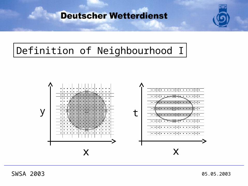
Assumption: LM-forecasts within a spatio-temporal neighbourhood are assumed to constitute a sample of the forecast at the central grid point

Neighbourhood Method

05.05.2003SWSA 2003

xx

Definition of Neighbourhood I

y t

05.05.2003SWSA 2003

Definition of Neighbourhood II

Size of Area

Formof Area

LinearRegressions

hs

05.05.2003SWSA 2003

Definition of the Quantile Function

The quantile function x is a function of probability p.

If the forecast is distributed according to the probability distributionfunction F, then

x(p) := F-1(p) for all p [0, 1].

There is a probability p that the quantile x(p) is greater than thecorrect forecast.

(Method according to Moon & Lall, 1994)

05.05.2003SWSA 2003

Products

„Statistically smoothed” fields• Quantiles for p = 0.5• Expectation Values

Probabilistic Information• Quantiles• (Probabilities for certain threshold values)

05.05.2003SWSA 2003

LM Total Precipitation [mm/h] 08.Sept.2001, 00 UTC, vv=14-15 h

Original Forecast Expectation Values

05.05.2003SWSA 2003

LM Total Precipitation [mm/h] 08.Sept.2001, 00 UTC, vv=14-15 h

Original Forecast Quantiles for p=0.9

05.05.2003SWSA 2003

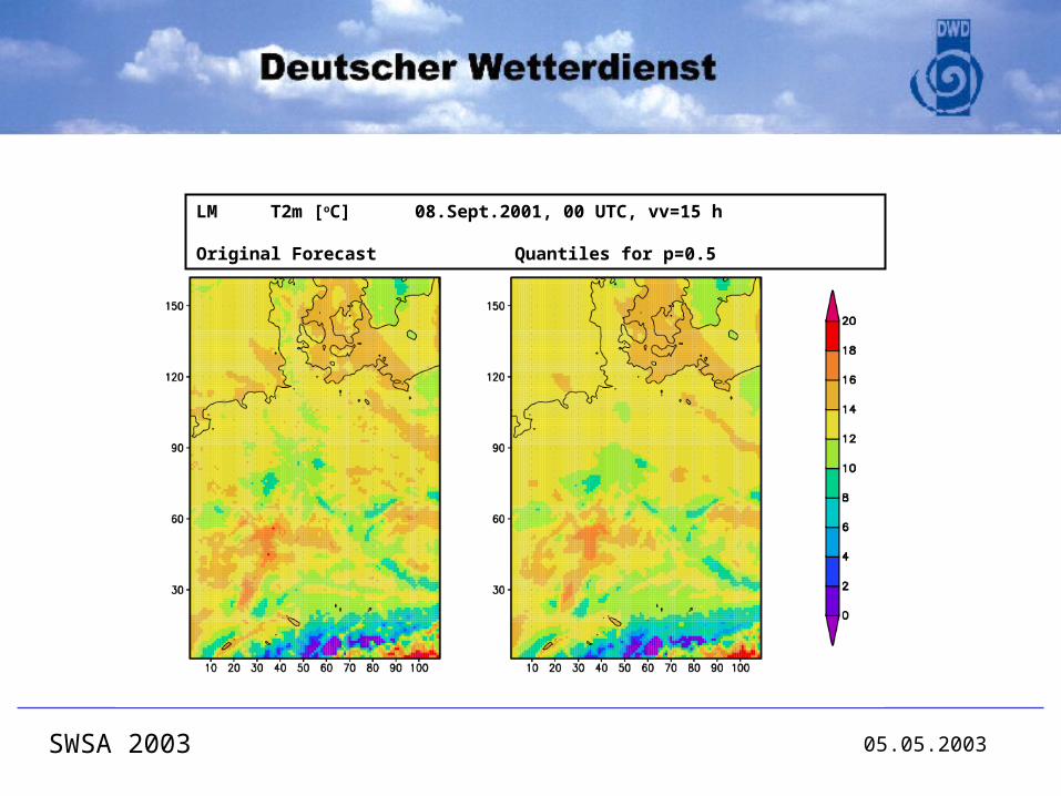
LM T2m [oC] 08.Sept.2001, 00 UTC, vv=15 h

Original Forecast Quantiles for p=0.5

05.05.2003SWSA 2003

Direct model output of the LM for precipitationat a given grid point

05.05.2003SWSA 2003

...supplemented by the 50 %-quantile

05.05.2003SWSA 2003

...supplemented by more quantiles(forecast of uncertainty)

05.05.2003SWSA 2003

...supplemented by the 90 %-quantile(forecast of risk)

05.05.2003SWSA 2003

DataLM forecasts; 1.-15.09.2001; 00 UTC starting time1 h values; 6-30 h forecast timeall SYNOPs available from German stationscomparison with nearest land grid point

NM-Versionssmall: 3 time levels (3 h); radius: 3s ( 20 km)medium: 3 time levels (3 h); radius: 5s ( 35 km)large: 7 time levels (7 h); radius: 7s ( 50 km)

Averagingsquare areas of different sizestemperatures adjusted with -0.65 K/(100 m)

Verification

05.05.2003SWSA 2003

RMSE(T) for 3 NM-Versions(0.5-Quantiles)

1.1

1.2

1.3

1.4

small medium large

[K]

RMSE(T) for VariousArea Averages

1.1

1.2

1.3

1.4

original 3x3 5x5 7x7 9x9 11x11

[K]

05.05.2003SWSA 2003

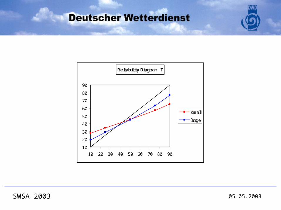
Reliability Diagram T

10

20

30

40

50

60

70

80

90

10 20 30 40 50 60 70 80 90

small

05.05.2003SWSA 2003

Richardson, D.S., 2001: Measures of skill and value of ensemble prediction systems, their interrelationshipand the effect of ensemble size. Q.J.R.Meteorol.Soc., Vol.127, pp. 2473-2489)

05.05.2003SWSA 2003

Reliability Diagram T

10

20

30

40

50

60

70

80

90

10 20 30 40 50 60 70 80 90

small

large

05.05.2003SWSA 2003

FBI for Various Area Averages

0.0

0.5

1.0

1.5

2.0

0.1 0.2 0.5 1 2 5

Precipitation Threshold in mm/h

original

3x3

5x5

7x7

9x9

11x11

05.05.2003SWSA 2003

TSS for Various Area Averages

05

10152025303540

0.1 0.2 0.5 1 2 5

Precipitation Threshold in mm/h

original

3x3

5x5

7x7

9x9

11x11

05.05.2003SWSA 2003

HSS for Various Area Averages

0

5

10

15

20

25

30

35

0.1 0.2 0.5 1 2 5

Precipitation Threshold in mm/h

original

3x3

5x5

7x7

9x9

11x11

05.05.2003SWSA 2003

ETS for Various Area Averages

0

5

10

15

20

0.1 0.2 0.5 1 2 5

Precipitation Threshold in mm/h

original

3x3

5x5

7x7

9x9

11x11

05.05.2003SWSA 2003

LOR for Various Area Averages

1.0

1.5

2.0

2.5

3.0

3.5

4.0

4.5

0.1 0.2 0.5 1 2 5

Precipitation Threshold in mm/h

original

3x3

5x5

7x7

9x9

11x11

05.05.2003SWSA 2003

FBI for 3 NM-Versions (Exp. Values)

0.0

0.5

1.0

1.5

2.0

2.5

0.1 0.2 0.5 1 2 5

Precipitation Threshold in mm/h

original

small

medium

large

11x11

05.05.2003SWSA 2003

ETS for 3 NM-Versions (Exp. Values)

0

5

10

15

20

0.1 0.2 0.5 1 2 5

Precipitation Threshold in mm/h

original

small

medium

large

11x11

05.05.2003SWSA 2003

FBI for 3 NM-Versions (0.5-Quantiles)

0.0

0.5

1.0

1.5

2.0

0.1 0.2 0.5 1 2 5

Precipitation Threshold in mm/h

original

small

medium

large

11x11

05.05.2003SWSA 2003

ETS for 3 NM-Versions (0.5-Quantiles)

0

5

10

15

20

25

0.1 0.2 0.5 1 2 5

Precipitation Threshold in mm/h

original

small

medium

large

11x11

05.05.2003SWSA 2003

Reliability Diagram RR(0.1-Quantile >= 0.1 mm/h)

10

20

30

40

50

60

70

80

90

10 20 30 40 50 60 70 80 90

small

medium

large

05.05.2003SWSA 2003

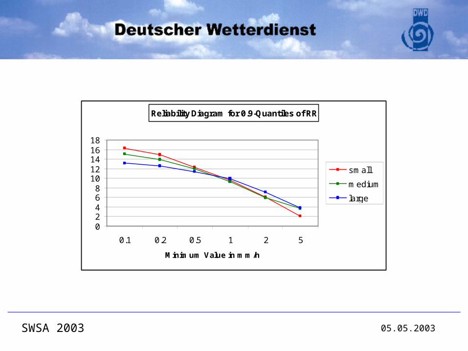
Reliability Diagram for 0.9-Quantiles of RR

02468

1012141618

0.1 0.2 0.5 1 2 5

Minimum Value in mm/h

small

medium

large

05.05.2003SWSA 2003

Reliability Diagram for 0.9-Quantiles of RR

0

5

10

15

20

25

30

0.1 0.2 0.5 1 2 5

Minimum Value in mm/h

small

medium

large

chance

05.05.2003SWSA 2003

Calibration

• Empirical Approach: use a large data sets of forecasts and observations

PRO: covers all relevant effectsCON: calibration is dependent on LM-version

• Theoretical Approach: focus on the effect of limited sample size only

PRO: effect can be quantified theoretically, without large data setscalibration is independent of LM-version

CON: all other effects are neglected

05.05.2003SWSA 2003

Calibration Procedure:

• choose probability p of the desired quantile (e.g. p=90%, if you would like to estimate the 90%-quantile)

• determine sample size M, frequency of the event and predictability of the event (a priori)

• calculate a probability p' = p' (p,M,,) from statistical theory (Richardson, 2001), let‘s say p' = 95% • estimate 95%-quantile and redefine it as a 90%-quantile

05.05.2003SWSA 2003

Richardson, D.S., 2001: Measures of skill and value of ensemble prediction systems, their interrelationshipand the effect of ensemble size. Q.J.R.Meteorol.Soc., Vol.127, pp. 2473-2489)

p

p'

05.05.2003SWSA 2003

Preliminary Results of Calibration (small neighbourhood):

Determination ofp' = p' (p,M,,) :

integrate p' = p' (p,M,,) over all possible values of and and over M=[1,80]

(LM forecasts; 10.-24.07.2002; 00 UTC starting time)

05.05.2003SWSA 2003

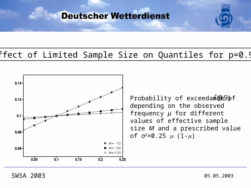
Effect of Limited Sample Size on Quantiles for p=0.9

Probability of exceedance of depending on the observed frequency μ for different values of effective sample size M and a prescribed value of σ2=0.25 (1-)

)9.0(x̂

05.05.2003SWSA 2003

Concluding Remarks

“Statistically Smoothed” Fields

For temperature no mean advantage is to be seen in comparison with simple averaging

The results for precipitation are difficult to judge upon; proper choice amongst the various possibilities is still an open question

Reliability Diagrams

Possible improvement by calibration remains to be explored

The results for precipitation clearly demonstrate the need for improving the model (reduce the overforecasting of slight precipitation amounts)

05.05.2003SWSA 2003

Concluding Remarks (ctd.)

Application

The method might be useful not only for single forecasts but also in combination with small ensembles