statistical physics of a model binary genetic switch with...

Statistical physics of a model binary genetic switch with linear feedback

Paolo Visco, Rosalind J. Allen, and Martin R. EvansSUPA, School of Physics and Astronomy, The University of Edinburgh, James Clerk Maxwell Building,

The King’s Buildings, Mayfield Road, Edinburgh EH9 3JZ, United Kingdom�Received 19 December 2008; published 30 March 2009�

We study the statistical properties of a simple genetic regulatory network that provides heterogeneity withina population of cells. This network consists of a binary genetic switch in which stochastic flipping between thetwo switch states is mediated by a “flipping” enzyme. Feedback between the switch state and the flipping rateis provided by a linear feedback mechanism: the flipping enzyme is only produced in the on switch state andthe switching rate depends linearly on the copy number of the enzyme. This work generalizes the model ofVisco et al. �Phys. Rev. Lett. 101, 118104 �2008�� to a broader class of linear feedback systems. We present acomplete analytical solution for the steady-state statistics of the number of enzyme molecules in the on and offstates, for the general case where the enzyme can mediate flipping in either direction. For this general case wealso solve for the flip time distribution, making a connection to first passage and persistence problems instatistical physics. We show that the statistics are non-Poissonian, leading to a peak in the flip time distribution.The occurrence of such a peak is analyzed as a function of the parameter space. We present a relation betweenthe flip time distributions measured for two relevant choices of initial condition. We also introduce a correla-tion measure and use this to show that this model can exhibit long-lived temporal correlations, thus providinga primitive form of cellular memory. Motivated by DNA replication as well as by evolutionary mechanismsinvolving gene duplication, we study the case of two switches in the same cell. This results in correlationsbetween the two switches; these can be either positive or negative depending on the parameter regime.

DOI: 10.1103/PhysRevE.79.031923 PACS number�s�: 87.18.Cf, 87.16.Yc, 82.39.�k

I. INTRODUCTION

Populations of biological cells frequently show stochasticswitching between alternative phenotypic states. This phe-nomenon is particularly well studied in bacteria and bacte-riophages, where it is known as phase variation �1�. Phasevariation often affects cell surface features, and its evolution-ary advantages are believed to involve evading attack fromhost defense systems �e.g., the immune system� and/or “bet-hedging” against sudden catastrophes which may wipe out aparticular phenotypic type. Switching between different phe-notypic states is controlled by an underlying genetic regula-tory network, which randomly flips between alternative pat-terns of gene expression. Several different types of geneticnetwork are known to control phase variation—these includeDNA inversion switches, DNA methylation switches, andslipped strand mispairing mechanisms �1–3�.

In this paper, we study a simple model for a genetic net-work that allows switching between two alternative states ofgene expression. Its key feature is that it includes a linearfeedback mechanism between the switch state and the flip-ping rate. When the switch is active, an enzyme is producedand the rate of switching is linearly proportional to the copynumber of this enzyme. The statistical properties of thismodel are made nontrivial by this feedback, leading, amongother things, to non-Poissonian behavior that may be of ad-vantage to cells in surviving in certain dynamical environ-ments. Our model is very generic and does not aim to de-scribe any specific molecular mechanism in detail, but ratherto determine in a general way the consequences of the linearfeedback for the switching statistics. Motivated by the factthat cells often contain multiple copies of a particular geneticregulatory element, due to DNA replication or DNA duplica-

tion events during evolution, we also consider the case oftwo identical switches in the same cell. We find that the twocopies of the switch are coupled and may exhibit interestingand potentially important correlations or anticorrelations.Our model switch is fundamentally different from bistablegene networks that have been the subject of previous theo-retical interest. In fact, as we shall show, our switch is notbistable but is intrinsically unstable in each of its two states.

Before discussing our model in detail, we provide a briefoverview of the basic biology of genetic networks and sum-marize some previously considered models for geneticswitches. Genetic networks are interacting many-componentsystems of genes, RNA, and proteins that control the func-tions of living cells. Genes are stretches of DNA ��1000base pairs long in bacteria�, whose sequences encode particu-lar protein molecules. To produce a protein molecule, theenzyme complex RNA polymerase copies the gene sequenceinto a messenger RNA �mRNA� molecule. This is known astranscription. The mRNA is then translated �by a ribosomeenzyme complex� into an amino acid chain which folds toform the functional protein molecule. The production of aspecific set of proteins from their genes ultimately deter-mines the phenotypic behavior of the cell. Phenotypic behav-ior can thus be controlled by turning genes on and off. Regu-lation of transcription �production of mRNA� is oneimportant way of achieving this. Transcription is controlledby the binding of proteins known as transcription factors tospecific DNA sequences, known as operators, usually situ-ated at the beginning of the gene sequence. These transcrip-tion factors may be activators �which enhance the transcrip-tion of the gene they regulate� or repressors �which represstranscription, often by preventing RNA polymerase binding�.A given gene may encode a transcription factor that regulates

PHYSICAL REVIEW E 79, 031923 �2009�

1539-3755/2009/79�3�/031923�16� ©2009 The American Physical Society031923-1

http://dx.doi.org/10.1103/PhysRevE.79.031923

itself or other genes, leading to complex networks of tran-scriptional interactions between genes.

There has been much recent interest among both physicalscientists and biologists in deconstructing complex geneticnetworks into modular units �4�, and in seeking to under-stand their statistical properties using theory and simulation�5,6�. Of particular interest is the fact that genetic networksare intrinsically stochastic, due to the small numbers of mol-ecules involved in gene expression �7,8�. This can give riseto heterogeneity in populations of genetically and environ-mentally identical cells �7�. For some genetic networks, thisheterogeneity is “all or nothing:” the population splits intotwo distinct subpopulations, with different states of gene ex-pression. Such networks are known as bistable geneticswitches: they have two possible long-time states, corre-sponding to alternative phenotypic states. Well-known ex-amples are the switch controlling the transition from thelysogenic to lytic states in bacteriophage � �9,10�, and thelactose utilization network of the bacterium Escherichia coli�11�. Several simple mechanisms for achieving bistabilityhave been studied, including pairs of mutually repressinggenes �12,13�, positive feedback loops �14�, and mixed feed-back loops �15�. Such bistable genetic networks can allowlong-lived and binary responses to short-lived signals—forexample, when a cell is triggered by a transient signal tocommit to a particular developmental pathway.

Theoretical treatments of bistable genetic networks usu-ally consider the dynamics of the copy number �or concen-tration� of the regulatory proteins involved. This affects theactivation state of the genes, which in turn influences the rateof protein production. The macroscopic rate equation ap-proach �16� provides a deterministic �mean-field� descriptionof the dynamics that ignores fluctuations in protein copynumber or gene expression state. This approach, applied to aswitch with two mutually repressing genes, has shown thatcooperative binding of regulatory proteins is an importantfactor in generating bistability �13�. Other studies haveshown, however, that bistability can be achieved even whenthe deterministic equations have only one solution, due tostochasticity and fluctuations in protein numbers �17,18�. Analternative approach is to study the dynamics of stochasticflipping between two stable states using stochastic simula-tions �19–21�, by numerically integrating the master equation�22�, or by path-integral-type approaches �23�. This dynami-cal problem bears some resemblance to the Kramers problemof escape from a free-energy minimum �24,25�. One there-fore expects on general grounds that the typical time spent inone of the bistable states should be exponentially large in thetypical number of proteins present in the state. This has beenconfirmed, at least for cooperative toggle switches formed ofmutually repressing genes �19,20�. From the perspective ofstatistical physics, interesting questions arise concerning thedistribution of escape times and the connection to first pas-sage properties of stochastic processes.

In this paper, however, we are concerned with an intrin-sically different situation from these bistable genetic net-works. The molecular mechanisms controlling microbialphase variation typically involve a binary element that can bein either of two states. For example, this may be a shortfragment of DNA that can be inserted into the chromosome

in either of two orientations, a repeated DNA sequence thatcan be altered in its number of repeats, or a DNA sequencethat can have two alternative patterns of methylation �1�. Theflipping of this element between its two states is stochastic,with a flipping rate that is controlled by various regulatoryproteins, the activity of which may be influenced by environ-mental factors. We shall consider the case where a feedbackexists between the switch state and the flipping rate. This isparticularly interesting from a statistical physics point ofview because it leads to non-Poissonian switching behavior,as we shall show. Our work has been motivated by severalexamples. The fim system in uropathogenic strains of thebacterium E. coli controls the production of type-1 fimbriae�or pili�, which are “hairs” on the surface of the bacterium.Individual cells switch stochastically between “on” and “off”states of fimbrial production �1,26–28�. The key feature ofthe fim switch is a short piece of DNA that can be insertedinto the bacterial DNA in two possible orientations. Becausethis piece of DNA contains the operator sequence for theproteins that make up the fimbriae, in one orientation, thefimbrial genes are transcribed and fimbriae are produced �theon state� and in the other orientation, the fimbrial genes arenot active and no fimbriae are produced �the off state�. Theinversion of this DNA element is mediated by recombinaseenzymes. Feedback between the switch state and the switch-flipping rate arises because the FimE recombinase �whichflips the switch in the on-to-off direction� is produced morestrongly in the on switch state than in the off state. Thisphenomenon is known as orientational control �29–31�. Theproduction of a second type of fimbriae in uropathogenic E.coli, Pap pili, also phase varies, and is controlled by a DNAmethylation switch �1,2,32�. Here, the operator region for thegenes encoding the Pap pili can be in two states, in which theDNA is chemically modified �methylated� at different sites,and different binding sites are occupied by the regulatoryprotein Lrp. Switching in this system is facilitated by thePapI protein, which helps Lrp to bind �33�. Feedback be-tween the switch state and the flipping rate arises because theproduction of PapI itself is activated by the protein PapB,which is only produced in the on state �1,2,34�.

A common feature of the above examples is the existenceof a feedback mechanism: in the fim system this occursthrough orientational control, and in the pap system, throughactivation of the papI gene by PapB. In this paper, we aim tostudy the role of such feedback within a simple, genericmodel of a binary genetic switch. We shall assume that thefeedback is linear, and we thus term our model a “linearfeedback switch.” In a recent publication �35�, we presenteda simple mathematical model of a DNA inversion geneticswitch with orientational control, which was inspired by thefim system. Our model reduces to the dynamics of the num-ber of molecules of a “flipping enzyme” R, which mediatesswitch flipping, along with a binary switch state. Enzyme Ris produced only in the on switch state. As the copy numberof R increases, the on-to-off flipping rate of the switch in-creases and this results in a non-Poissonian flipping processwith a peak in the lifetime of the on state. The model is linearin the sense that the rate at which the switch is turned off isa linear function of the number of enzymes R which it pro-duces. In our previous work �35�, we imagined enzyme R to

VISCO, ALLEN, AND EVANS PHYSICAL REVIEW E 79, 031923 �2009�

031923-2

be a DNA recombinase, and the two switch states to corre-spond to different DNA orientations, in analogy with the fimsystem. However, the same model could be used to describea range of molecular mechanisms for binary switch flippingwith feedback between the switch state and flipping rate, andcan thus be considered a generic model of a genetic switchwith linear feedback.

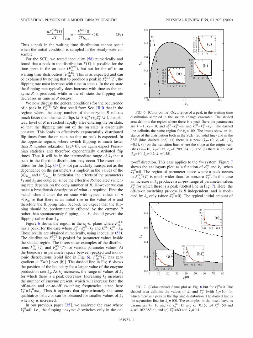
In our recent work �35�, we obtained exact analytical ex-pressions for the steady-state enzyme copy number for ourmodel switch with linear feedback, in the particular casewhere the flipping enzyme switches only in the on-to-offdirection �this being the relevant case for fim�. We also cal-culated the flip time distribution for this model analytically.Conceptually, such a calculation is reminiscent of the studyof persistence in statistical physics �36� where, for example,one asks about the probability that a spin in an Ising systemhas not flipped up to some time �37�. For the flip time dis-tribution, we defined different measurement ensembles ac-cording to whether one starts the time measurement from aflip event �the switch change ensemble �SCE�� or from arandomly selected time �the steady-state ensemble �SSE��. Inthe present paper, we extend this work to present the fullsolution of the general case of the model and extend ourstudy of its persistence properties. The presence of a rate forthe enzyme-mediated off-to-on flipping �k3

off� has most sig-nificant effects on the flip time distributions F�T�, as illus-trated in Figs. 6 and 7, where we show the parameter rangeover which a peak is found in F�T� for zero and nonzero k3

off.We also prove an important relation between the two mea-surement ensembles defined in �35� and use it to show that apeak in the flip time distribution only occurs in the switchchange ensemble and not in the steady-state ensemble. Wefind that the non-Poissonian behavior of this model switchleads to interesting two-time autocorrelation functions. Wealso study the case where we have two copies of the switchin the same cell and find that these two copies may be cor-related or anticorrelated, depending on the parameters of themodel, with potentially interesting biological implications.

The paper is structured as follows. In Sec. II we define themodel, describe its phenomenology, and show that a “mean-field” deterministic version of the model has only onesteady-state solution. In Sec. III we present the general solu-tion for the steady-state statistics, and in Sec. IV we studyfirst-passage time properties of the switch; technical calcula-tions are left to Appendixes A and B. In Sec. V we considertwo coupled model switches and we present our conclusionsin Sec. VI.

II. MODEL

We consider a model system with a flipping enzyme Rand a binary switch S, which can be either on or off �de-noted, respectively, as Son and Soff�. Enzyme R is produced�at rate k2� only when the switch is in the on state, and isdegraded at a constant rate k1, regardless of the switch state.This represents protein removal from the cell by dilution oncell growth and division, as well as specific degradationpathways. Switch flipping is assumed to be a single-step pro-cess, which either can be catalyzed by enzyme R, with rate

constants k3on and k3

off and linear dependence on the numberof molecules of R, or can happen “spontaneously,” with ratesk4

on and k4off. We imagine that the spontaneous switching pro-

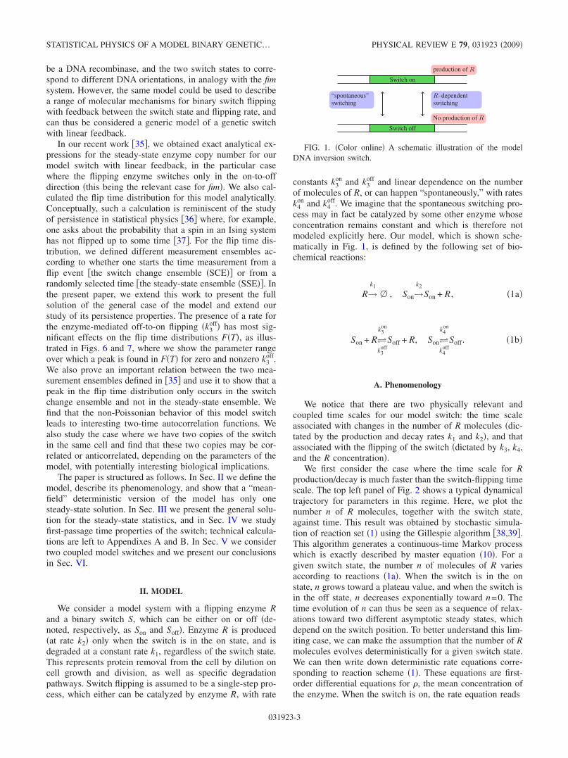
cess may in fact be catalyzed by some other enzyme whoseconcentration remains constant and which is therefore notmodeled explicitly here. Our model, which is shown sche-matically in Fig. 1, is defined by the following set of bio-chemical reactions:

R→k1

� , Son→k2

Son + R , �1a�

Son + R�k3

off

k3on

Soff + R, Son�k4

off

k4on

Soff. �1b�

A. Phenomenology

We notice that there are two physically relevant andcoupled time scales for our model switch: the time scaleassociated with changes in the number of R molecules �dic-tated by the production and decay rates k1 and k2�, and thatassociated with the flipping of the switch �dictated by k3, k4,and the R concentration�.

We first consider the case where the time scale for Rproduction/decay is much faster than the switch-flipping timescale. The top left panel of Fig. 2 shows a typical dynamicaltrajectory for parameters in this regime. Here, we plot thenumber n of R molecules, together with the switch state,against time. This result was obtained by stochastic simula-tion of reaction set �1� using the Gillespie algorithm �38,39�.This algorithm generates a continuous-time Markov processwhich is exactly described by master equation �10�. For agiven switch state, the number n of molecules of R variesaccording to reactions �1a�. When the switch is in the onstate, n grows toward a plateau value, and when the switch isin the off state, n decreases exponentially toward n=0. Thetime evolution of n can thus be seen as a sequence of relax-ations toward two different asymptotic steady states, whichdepend on the switch position. To better understand this lim-iting case, we can make the assumption that the number of Rmolecules evolves deterministically for a given switch state.We can then write down deterministic rate equations corre-sponding to reaction scheme �1�. These equations are first-order differential equations for �, the mean concentration ofthe enzyme. When the switch is on, the rate equation reads

Switch off

No production of R

“spontaneous”switching

R–dependentswitching

Switch on

production of R

FIG. 1. �Color online� A schematic illustration of the modelDNA inversion switch.

STATISTICAL PHYSICS OF A MODEL BINARY GENETIC… PHYSICAL REVIEW E 79, 031923 �2009�

031923-3

d�

dt= − k1� + k2, �2�

with solution

��t� = ��0�e−k1t +k2

k1�1 − e−k1t� . �3�

Thus the plateau density in the on state is given by the ratio

�on = k2/k1, �4�

and the time scale for relaxation to this density is given byk1, the rate of degradation of R1. When the switch is in theoff state, the rate equation for � reads instead

d�

dt= − k1� , �5�

and one simply has exponential decay to �=0 with decaytime k1. In this parameter regime, switch flipping typicallyhappens when the number of molecules of R has alreadyreached the steady state �as in the top left panel of Fig. 2�.Thus, the on-to-off switching time scale is given by1 / ��onk3

on+k4on�, where �on is the plateau concentration of

flipping enzyme when the switch is in the on state, given byEq. �4�. Since the corresponding plateau concentration in theoff switch state is zero, the off-to-on switch-flipping timescale is simply given by 1 /k4

off.We now consider the opposite scenario, in which switch-

ing occurs on a much shorter time scale than relaxation ofthe enzyme copy number. A typical trajectory for this case isshown in the bottom left panel of Fig. 2. Here, switchingreactions dominate the dynamics of the model, and the dy-namics of the enzyme copy number follows a standard birth-death process, with an effective birth rate given by the en-zyme production rate in the on state multiplied by thefraction of time spent in the on state. A more quantitativeaccount for these behaviors is provided later on, in Sec.III B.

For parameter values between these two extremes, wherethe time scales for switch flipping and enzyme number re-laxation are similar, it is more difficult to provide intuitiveinsights into the behavior of the model. A typical trajectoryfor this case is given in the middle left panel of Fig. 2. Here,we have set the on-to-off and off-to-on switching rates to beidentical: k3

on=k3off and k4

on=k4off. We notice that typically, less

time is spent in the on state than in the off state. As soon asthe switch flips into the on state, the number of R moleculesstarts increasing and the on-to-off flip rate begins to increase.Consequently, the number of R molecules rarely reaches itsplateau value before the switch flips back into the off state.

To illustrate the effects of including the parameter k3off, we

also show trajectories for different values of the ratio r=k3

off /k3on in Fig. 3, for fixed k3

on. For small r, the amount ofenzyme decays to zero in the off state before the next off-to-on flipping event, resulting in bursts of enzyme produc-tion. In contrast, when r is O�1�, flipping is rapid in bothdirections so that p�n� is peaked at intermediate n.

B. Mean-field equations

To explore how the switching behavior of our modelarises, we can write down mean-field deterministic rate equa-tions corresponding to the full reaction scheme �1�. Theseequations describe the time evolution of the mean concentra-tion ��t� of R molecules and the probabilities Qon�t� andQoff�t� of the switch being in the on and off states. Theseequations implicitly assume that the mean enzyme concen-tration � is completely decoupled from the state of theswitch. Thus correlations between the concentration � andthe switch state are ignored and the equations furnish amean-field approximation for the switch. As we now show,this crude type of mean-field description is insufficient todescribe the stochastic dynamics of the switch, except in thelimit of high flipping rate. Noting that Qon�t�+Qoff�t�=1, themean-field equations read

FIG. 2. �Color online� Left: typical trajectories of the system when k3on=k3

off=k3 is increased �from top to bottom k3=0.0001, 0.01, and1�. The other parameters are k1=1, k2=100, and k4

on=k4off=k4=0.1. Gray shading denotes periods in which the switch is in the on state, and

the solid lines denote the number of enzyme molecules, plotted against time. In the bottom panel, the switch flips so fast that the gray shadingis only shown in the inset where the trajectory from k1t= �60,61� is shown in detail. Right: probability distribution functions for the numbern of R molecules, for parameter values corresponding to the trajectories shown in the left panels. The symbols are the results of numericalsimulations �see text for details�. The full curves plot analytical results �26� and �36�, which are in perfect agreement with the simulations.


031923-4

d��t�dt

= k2Qon�t� − k1��t� , �6a�

dQon�t�dt

= �k4off + ��t�k3

off��1 − Qon�t�� − �k4on + ��t�k3

on�Qon�t� .

�6b�

The above equations have two sets of possible solutions forthe steady-state values of � and Qon, but only one has apositive value of �, and is therefore physically meaningful.The result is

� =�onk3

off − �k4off + k4

on� + ��

2�k3off + k3

on�, �7�

where

� = ��onk3off − �k4

off + k4on��2 + 4�onk4

off�k3off + k3

on� , �8�

and

Qon = �/�on. �9�

The most interesting conclusion to be drawn from this mean-field analysis is that there is only one physically meaningfulsolution. In this solution, the enzyme concentration � is lessthan the plateau value in the on state ��on of Eq. �4��. Thusreaction scheme �1� does not have an underlying bistability.The two states of our stochastic switch evident in Figs. 2 and4 for low values of k3 and k4 are not bistable states but arerather intrinsically unstable and transient states, each ofwhich will inevitably give rise to the other after a certain�stochastically determined� period of time. In this sense, ourmodel is fundamentally different from the bistable reactionnetworks which have previously been discussed �13,19,40�.On the other hand, in the limit of rapid switch flipping,where k3 or k4 is large, the mean-field description holds andthe protein number distribution does show a single peakwhose position is well approximated by Eq. �7�, as shown inFigs. 2 and 4 for the case k3=1.

FIG. 3. �Color online� Left: Typical trajectories of the system when r=k3off /k3

on is increased �from top to bottom r=0, 0.5, and 1�. Theother parameters are k1=1, k2=100, k3

on=1, and k4on=k4

off=k4=0.1. Gray shading denotes periods in which the switch is in the on state, andthe solid lines denote the number of enzyme molecules, plotted against time. In the bottom panel, the switch flips so fast that the gray shadingis only shown in the inset where the trajectory from k1t= �60,61� is shown in detail. Right: probability distribution functions for the numbern of R molecules, for parameter values corresponding to the trajectories shown in the left panels. The symbols are the results of numericalsimulations �see text for details�. The full curves plot analytical results �26� and �36�, which are in perfect agreement with the simulations.

FIG. 4. �Color online� Left: typical trajectories of the system when k4on=k4

off=k4 is increased �from top to bottom k4=0.1, 1, and 100�.Other parameters are k1=1, k2=100, and k3

on=k3off=k3=0.001. In each panel the gray shading denotes that the switch is on and the line plots

the number of enzymes against time. In the third panel the gray shading is only shown in the inset where the trajectory from k1t= �60,61� is detailed. Right: probability distribution functions of the number of R molecules in the cell for parameter values correspondingto the trajectories shown in the left panels. The symbols are the results of numerical simulations �see text for details�. The full curves plotanalytical results �26� and �36� and pass perfectly through the simulation points.


031923-5

III. STEADY-STATE STATISTICS

A. Analytical solution

Returning to the fully stochastic version of reactionscheme �1�, we now present an exact solution for the steady-state statistics of this model. A solution for the case wherek3

off=0 was sketched in Ref. �35�. Here we present a com-plete solution for the general case where k3

off�0, and wediscuss the properties of the steady-state as a function of allthe parameters of the system.

We first define the probability ps�n , t� that the system hasexactly n enzyme molecules at time t and the switch is in thes state �where s= �on,off��. The time evolution of ps is de-scribed by the following master equation:

dps�n�dt

= �n + 1�k1ps�n + 1� + k2s ps�n − 1� + nk3

1−sp1−s�n�

+ k41−sp1−s�n� − �nk1 + k2

s + nk3s + k4

s�ps�n� , �10�

where we use the shorthand notations �off,on��0,1�, k2off

0, and k2onk2. In the steady state, the time derivative in

Eq. �10� vanishes, and the problem reduces to a pair ofcoupled equations for pon and poff:

�n + 1�k1pon�n + 1� + k2pon�n − 1� + nk3offpoff�n� + k4

offpoff�n�

= �nk1 + k2 + nk3on + k4

on�pon�n� , �11a�

�n + 1�k1poff�n + 1� + nk3onpon�n,t� + k4

onpon�n,t�

= �nk1 + nk3off + k4

off�poff�n,t� . �11b�

To solve the above equations we use the generating functions

Gs�z� = n=0

�

ps�n�zn. �12�

The steady-state equations �11� can be now written as a set oflinear coupled differential equations for Gs:

L1Gon�z� = L2Goff�z� , �13a�

L3Goff�z� = L4Gon�z� , �13b�

where Li are linear differential operators

L1�z� = k1�z − 1��z − k2�z − 1� + k3onz�z + k4

on, �14a�

L2�z� = k3offz�z + k4

off, �14b�

L3�z� = k1�z − 1��z + k3offz�z + k4

off, �14c�

L4�z� = k3onz�z + k4

on. �14d�

In order to solve the two coupled Eqs. �13a� and �13b� it isfirst useful to take their difference. After simplification thisyields the relation

�zGoff�z� = − �zGon�z� +k2

k1Gon�z� . �15�

Next, we take the first derivative of Eq. �13b� and then re-place the derivatives of Goff with relation �15�. After some

algebra, one finds that Gon verifies the second-order differen-tial equation

k1��z − k1�Gon� �z� + �k1� − �z�Gon� �z� − Gon�z� = 0,

�16�

where the Greek letters are combinations of the parametersof the model:

� = k1 + k3on + k3

off, �17a�

� = k1 + k2 + k3off + k3

on + k4off + k4

on, �17b�

� = k2�k1 + k3off� , �17c�

= k2�k1 + k3off + k4

off� . �17d�

We now define the variable

u�z� uz =�

k1�z −

�

�2 = u0 + z�u1 − u0� , �18�

and the parameter combinations

= u0 +�

�, � =

�. �19�

We can now write Gon�z� �and Goff�z�� in terms of the vari-able u �Eq. �18�� by defining the functions

Js�u� = Gs�z� . �20�

Differential equation �16� then reads

uJon� �u� + � − u�Jon� �u� − �Jon�u� = 0. �21�

Looking for a regular power-series solution of the form

Jon�u� = n=0

�

anun, �22�

one obtains the following solution:

Jon�u� = a0 1F1��,,u� , �23�

where 1F1 denotes the confluent hypergeometric function ofthe first kind,

1F1��,,u� n=0

��n

��n

un

n!�24�

and ��n=��+1�¯ ��+n−1� denotes the Pochhammersymbol.

The constant a0 will be determined using the boundaryconditions, which we discuss later. We first note that theabove result for Jon�u� can be translated into Gon�z� by re-placing u with the expression of u�z� in Eq. �22� and expand-ing in powers of z:


031923-6

Gon�z� = n=0

�

an�u0 + z�u1 − u0��n

= n=0

�

anm=0

n

u0m�z�u1 − u0��n−m� n

m�

= n=0

�

znm=n

�

amu0m−n��u1 − u0��n�m

n� , �25�

where we have relabeled the indices n−m→n and n→m inthe last equality of Eq. �25�. We can identify pon�n� from Eq.�12� as the coefficient of zn in the above expression:

pon�n� = m=n

�

amu0m−n�u1 − u0�n�m

n� . �26�

From Eqs. �22� and �23� we read off

an =a0

n!

��n

��n. �27�

Substituting Eq. �27� into Eq. �26� we deduce, using thedefinition of the hypergeometric function �24� and noting��n+m= ��n��+n�m, that

pon�n� = a0�u1 − u0�n

n!

��n

��n1F1�� + n, + n,u0� . �28�

In deriving this expression we have, in fact, established thefollowing identity, which will prove useful again later:

1F1��,,u� = n=0

�zn�u1 − u0�n

n!

��n

��n1F1�� + n, + n,u0� .

�29�

To compute Goff�z�, we integrate Eq. �15�, which yields,using the form of Jon�u� �Eq. �23��

Goff�z� + Gon�z� − a0k2� − 1�

k1�� − 1��u1 − u0� 1F1�� − 1, − 1,uz�

= � , �30�

where � is our second integration constant. We then havetwo constants, a0 and �, which still need to be determined.The constant � can be found using the normalization condi-tion n�pon�n�+ poff�n��=1, which is equivalent to Gon�1�+Goff�1�=1. Using this condition, we obtain

� = 1 − a0k2� − 1�

k1�� − 1��u1 − u0� 1F1�� − 1, − 1,u1� . �31�

In order to compute the remaining constant a0, we considerthe boundary condition at z=0. From definition �12� of thegenerating function we see that Gs�z=0�= ps�n=0�. Ourboundary condition thus reads

Jon�u0� + Joff�u0� = pon�0� + poff�0� . �32�

Setting n=0 in master equation �11a� �noting that the term inpon�n−1� vanishes� gives poff�0� in terms of pon�0� andpon�1�:

poff�0� =k2 + k4

on

k4off pon�0� −

k1

k4off pon�1� . �33�

Combining Eq. �30� �with z=0� and Eq. �31�, substitutinginto Eq. �32�, using Eq. �33� to eliminate poff�0�, and finallysubstituting in expressions for pon�0� and pon�1� from Eq.�26�, we determine a0:

a0−1 = �1 +

k2 + k4on

k4off �1F1��,,u0� −

k1��u1 − u0�k4

off

1F1�� + 1, + 1,u0� −k2� − 1�

k1�� − 1��u1 − u0�

�1F1�� − 1, − 1,u0� − 1F1�� − 1, − 1,u1�� .

�34�

The final step in obtaining our exact solution is to provide anexplicit expression for poff�n�. From Eq. �30� we have

Goff�z� = � − Gon�z� + a0k2� − 1�

k1�� − 1��u1 − u0�

1F1�� − 1, − 1,uz� , �35�

and using identity �29� we obtain

poff�n� = �n,0 +a0

n! k2

k1�u1 − u0�n−1 ��n−1

��n−1

1F1�� + n − 1, + n − 1,u0�

− �u1 − u0�n ��n

��n1F1�� + n, + n,u0�� , �36�

where i,j is the Kronecker delta.Our exact analytical solution �26�, �34�, and �36� is veri-

fied by comparison to computer simulation results in theright panels of Figs. 2 and 4. Here, we plot the probabilitydistribution function for the total number of enzyme mol-ecules:

p�n� = pon�n� + poff�n� . �37�

Computer simulations of reaction set �1� were carried outusing Gillespie’s stochastic simulation algorithm �38,39�.Perfect agreement is obtained between the numerical andanalytical solutions, as shown in Figs. 2 and 4.

B. Properties of the steady state

Having derived the steady-state solution for p�n�, we nowanalyze its properties as a function of the parameters of themodel. We choose to fix our units of time by setting k1, thedecay rate of enzyme R, to be equal to unity �so our timeunits are k1

−1�. With these units, the plateau value for thenumber of enzyme molecules in the on switch state is givenby �on=k2. In this section, we will only analyze the casewhere �on=100. To further simplify our analysis, we set k3

on

=k3off=k3 and k4

on=k4off=k4 �a discussion of the case where

k3off=0 and k3

on�0 is provided in Ref. �35��. We then analyzethe probability distribution p�n� as a function of theR-dependent switching rate k3 and the R-independent switch-


031923-7

ing rate k4. The results are shown in the right-hand panels ofFigs. 2 and 4. We consider the three regimes discussed inSec. II A: that in which enzyme number fluctuations aremuch faster than switch flipping, that where the opposite istrue, and finally the regime where the two time scales aresimilar.

In the regime where switch flipping is much slower thanenzyme production/decay �k1� �k4

on+k2k3on /k1��, the prob-

ability distribution p�n� is bimodal. This is easily under-standable in the context of the typical trajectories shown inthe left top panels in Figs. 2 and 4: in this regime, the num-ber of molecules of R always reaches its steady-state valuebefore the next switch flip occurs. It follows then that pon�n�is a bell-shaped distribution peaked around k2 /k1, whilepoff�n� is highly peaked around zero, so that the total distri-bution p�n�= pon�n�+ poff�n� is bimodal.

In contrast, when switching occurs much faster than en-zyme number fluctuations, the probability distribution p�n� isunimodal and bell shaped, as might be expected from thetrajectories in the bottom left panels of Figs. 2 and 4. Asdiscussed in Sec. II A, in this regime the number of R mol-ecules behaves as a standard birth-death process with effec-tive birth rate given by k2 multiplied by the average time theswitch spends in the on state, and death rate k1. For such abirth-death process the steady-state probability p�n� is aPoisson distribution with mean given by the ratio of the birthrate to the death rate. To show that our analytical result re-duces to this Poisson distribution, we consider the casewhere enzyme-mediated switching dominates �as in Fig. 2�,so that both k3

off and k3on are much greater than k1. The

fraction of time spent in the on state is k3off / �k3

on+k3off�; thus

the effective birth rate is k2k3off / �k3

on+k3off�. In the limit

k3on→� and k3

off→� with r=k3off /k3

on constant, one finds that�→1, →1, and uz→k2rz / �k1�1+r��. Using the fact that

1F1�1,1 ,x�=ex, Eq. �23� gives, in this limit,

Gon�z� = a0 exp� k2rz

k1�1 + r�� , �38�

which is the generating function of a Poisson distributionwith mean k2k3

off / �k1�k3on+k3

off��. Plugging this result into Eq.�30� and taking again the limit k3→� �and using

1F1�0,0 ,x�=1� finally yields the result that p�n�= pon�n�+ poff�n� is indeed a Poisson distribution. The same approachcan be taken for the case of Fig. 4, where k3 is constant, andk4

on and k4off become very large. The probability distribution

p�n� then becomes a Poisson distribution with meank2k4

off / �k1�k4on+k4

off��. The above result is only valid whenr�0. In fact, as shown in Fig. 3, when r=0 the distributionof R is peaked at 0 and does not have a Poisson-type shape.

Finally, when there is no clear separation of time scalesbetween enzyme number fluctuations and switch flipping, thedistribution function for the number of enzyme moleculeshas a highly nontrivial shape, as shown in Figs. 2 and 4.

IV. FIRST-PASSAGE TIME DISTRIBUTION

We now calculate the first-passage time distribution forour model switch. We define this to be the distribution func-

tion for the amount of time that the switch spends in the onor off state before switching. This distribution is biologicallyrelevant, since it may be advantageous for a cell to spendenough time in the on state to synthesize and assemble thecomponents of the “on” phenotype �for example, fimbriae�,but not long enough to activate the host immune system,which recognizes these components. The calculation for thecase k3

off=0 was sketched in �35�. Here we provide a detailedcalculation of the flip time distribution in the more generalcase k3

off�0. We find that this dramatically reduces the pa-rameter range over which the flip time distribution has apeak. We demonstrate an important relation between the fliptime distributions for the two relevant choices of initial con-ditions �switch change ensemble and steady-state ensemble�.The first-passage time distribution is important and interest-ing from a statistical physics point of view as it is related to“persistence.” Generally, persistence is expressed as theprobability that the local value of a fluctuating field does notchange sign up to time t �36�. For the particular case of anIsing model, persistence is the probability that a given spindoes not flip up to time t. In our model, the switch state Splays the role of the Ising spin. For other problems, there hasbeen much interest in the long-time behavior of the persis-tence probability, which can often exhibit a power-law tail.In our case, however, we expect an exponential tail for thedistribution of time spent in the on state, because linear feed-back will cause the switch to flip back to the off state aftersome characteristic time. We are therefore interested not onlyin the tail of the first-passage time distribution, but also in itsshape over the whole time range.

A. Analytical results

We consider the probability Fs�T �n0�dT that if we beginmonitoring the switch at time t0 when there are n0 moleculesof the flipping enzyme R, it remains from time t0→ t0+T instate s, and subsequently flips in the time interval t0+T→ t0+T+dT. This probability is averaged over a given en-semble of initial conditions, determined by the experimentalprotocol for monitoring the switch. Mathematically, the ini-tial condition n0 for switch state s is selected according tosome probability Ws�n0� and we define

Fs�T� = n0

Fs�T�n0�Ws�n0� �39�

as the flip time distribution for the ensemble of initial con-ditions given by Ws�n0�.

The most obvious protocol would be to measure the in-terval T from the moment of switch flipping, so that thetimes t0 correspond to switch flips and the T are the durationsof the on or off switch states. We call this the switch changeensemble �SCE�. In this ensemble, the probability Ws

SCE ofhaving n molecules of R at the time t0 when the switch flipsinto the s state is

WsSCE�n� =

p1−s�n��nk31−s + k4

1−s�

n

p1−s�n��nk31−s + k4

1−s�, �40�


031923-8

where for notational simplicity, s= �1,0� represents �on,off�.The numerator of the right-hand side of Eq. �40� gives thesteady-state probability that there are n molecules present instate 1−s, multiplied by the flip rate into state s. The de-nominator normalizes Ws

SCE�n�.We also consider a second choice of initial condition,

which we denote the steady-state ensemble �SSE�. Here, theinitial time t0 is chosen at random for a cell that is in the sstate. This choice is motivated by practical considerations:experimentally, it is much easier to pick a cell which is in thes state and to measure the time until it flips out of the s state,than to measure the entire length of time a single cell spendsin the s state. The probability Ws

SSE of having n molecules ofR at time t0 is then the �normalized� steady-state distributionfor the s state:

WsSSE =

ps�n�

n

ps�n�. �41�

To compute the distribution F�T�, we first consider thesurvival probability hs

W�n , t� that, given that at time t=0�chosen according to ensemble W� the switch was in state s,at time t it is still in state s and has n molecules of enzyme R.As the ensemble W only enters through the initial condition,we may drop the superscript W in what follows. The evolu-tion equation for hs is the same as for ps�n , t�, but without theterms denoting switch flipping into the s state. This removesthe coupling between pon and poff that was present in evolu-tion equations �11�:

�

�thon�n,t� = �n + 1�k1hon�n + 1,t� + k2hon�n − 1,t�

− �nk1 + k2 + nk3on + k4

on�hon�n,t� , �42a�

�

�thoff�n,t� = �n + 1�k1hoff�n + 1,t�

− �nk1 + nk3off + k4

off�hoff�n,t� . �42b�

Introducing the generating function

h̃s�z,t� = n=0

�

znhs�n,t� , �43�

the above equations reduce to

�

�th̃on�z,t� = �k1 − �k1 + k3

on�z��zh̃on�z,t�

+ �k2z − �k2 + k4on��h̃on�z,t� , �44a�

�

�th̃off�z,t� = �k1 − �k1 + k3

off�z��zh̃off�z,t� − k4offh̃off�z,t� .

�44b�

We can relate h to F by noting that nhs�n , t�= h̃s�1, t� isthe total probability that the switch has not flipped up to timet. Hence,

Fs�t� = − �th̃s�1,t� . �45�

Equations �44� can be solved using the method of character-istics �41�. The result, detailed in Appendix A, is

h̃on�z,t� = e−�ontek2�on�z−k1�on��1−e−t/�on�

W̃�k1�on + e−t/�on�z − k1�on�� , �46�

where �on= �k1+k3on�−1 and �on=k4

on+k2�1−k1�on�. The func-

tion W̃ is the generating function for the distribution of en-zyme numbers W�n� at the starting time for the measure-ment:

W̃�z� = n

W�n�zn, �47�

where W refers to WSCE or WSSE. The function h̃off�z , t� canbe obtained in an analogous way: this produces the same

expression as for h̃on, but with k2 set to zero and with all “on”superscripts replaced by “off:”

h̃off�z,t� = e−k4offtW̃�k1�off + e−t/�off�z − k1�off�� , �48�

where �off= �k1+k3off�−1. We can then obtain the distributions

Fon�T� and Foff�T� by differentiating the above expressions,according to Eq. �45�:

Fon�T� = exp − ��on +1

�on�T + k2�on�1 − e−T/�on��

��oneT/�on + k2�k1�on − 1��

W̃�k1�on + e−T/�on�1 − k1�on�� + � 1

�on− k1�

W̃��k1�on + e−T/�on�1 − k1�on�� , �49�

Foff�T� = exp − �k4off +

1

�off�T�

�k4offeT/�offW̃�k1�off + e−T/�off�1 − k1�off��

+ � 1

�off− k1�W̃��k1�off + e−T/�off�1 − k1�off�� .

�50�

In the above expressions, the function W̃s is given for theSSE by

W̃sSSE = Gs�z�/Gs�1� , �51�


031923-9

and for the SCE by

W̃sSCE�z� =

k31−szG1−s� �z� + k4

1−sG1−s�z�k3

1−sG1−s� �1� + k41−sG1−s�1�

. �52�

B. Relation between SSE and SCE

We now show that a useful and simple relation can bederived between FSSE�T� and FSCE�T�. Let us imagine thatwe pick a random time t, chosen uniformly from the totaltime that the system spends in state s. The time t will fall intoan interval of duration T, as illustrated in Fig. 5. We can thensplit the interval T into the time T1 before t and the time T2after t, such that T1+T2=T.

We first note that the probability that our randomly chosentime t falls into an interval of length T is

Prob�T�dT =TFs

SCE�T�dT

�0

�

T�FsSCE�T��dT�

. �53�

Equation �53� expresses the fact that the probability distribu-tion for a randomly chosen flip time T is Fs

SCE�T�dT, but theprobability that our random time t falls into a given segmentis proportional to the length of that segment. Since the time Tis chosen uniformly, the probability distribution for T2, for agiven T, will also be uniform �but must be less than T�:

Prob�T2�T�dT =��T − T2�

TdT . �54�

One can now obtain FsSSE from Prob�T2 �T� by integrating Eq.

�54� over all possible values of T, weighted by relation �53�.This leads to the following relation between FSCE and FSSE:

FsSSE�T2� =

�T2

�

FsSCE�T��dT�

�0

�


. �55�

Taking the derivative with respect to T2 this can be recast as

dFsSSE�T�dT

= −Fs

SCE�T��T�SCE

, �56�

where �T�SCE is simply the mean duration of a period in theon state. We have verified numerically that expressions �49�and �50� for Fs

SSE�T� and FsSCE�T� derived above do indeed

obey relation �56�. This relation can also be understood interms of backward evolution equations as we discuss in Ap-pendix B.

C. Presence of a peak in F(T)

We now focus on the shape of the flip time distributionF�T�: in particular, whether it has a peak. A peak in Fon

SCE�T�could be biologically advantageous for two complementaryreasons. First, after the switch enters the on state there maybe some start-up period before the phenotypic characteristicsof the on state are established, so it would be wasteful forflipping to occur before the on state of the switch has becomeeffective. Second, the on state of the switch may elicit anegative environmental response, such as activation of thehost immune system, so that it might be advantageous toavoid spending too long a time in the on state. For example,in the case of the fim switch, a certain amount of time andenergy is required to synthesize fimbriae, and this effort willbe wasted if the switch flips back into the off state beforefimbrial synthesis is complete. On the other hand, too large apopulation of fimbriated cells would trigger an immune re-sponse from the host. The length of time each cell is in thefimbriated state therefore needs to be tightly controlled. Wenote that for bistable genetic switches and many other rareevent processes, waiting time distributions are exponential�on a suitably coarse-grained time scale�. This arises fromthe fact that the alternative stable states are time invariant insuch systems. The presence of a peak in Fon

SCE�T� for ourmodel switch indicates fundamentally different behavior,which occurs because the two switch states in our model aretime dependent.

The presence of a peak in the distribution F�T� requiresthe slope of F�T� at the origin to be positive. Applying thiscondition to the function Fon �Eq. �49��, we get

�k2k3on − �k4

on�2�W̃�1� − k3on�k1 + k3

on + 2k4on�W̃��1�

− �k3on�2W̃��1� � 0. �57�

Equation �47� allows us to expressing the derivatives of W̃�1�as functions of the moments of n, so that we finally get ourcondition as a relation between the mean and the variance ofthe initial ensemble:

k2k3on − �k4

on�2 − k3on�k1 + 2k4

on��n�Won− �k3

on�2�n2�Won� 0,

�58�

where �¯�Wondenotes an average taken using the weight Won

of Eq. �40� and �41�. Analogous conditions can be found fora peak in the off-to-on waiting time distribution. The mo-ments involved in the above inequality can be computed us-ing the exact results of Sec. III B. The left-hand side of Eq.�58� can then be computed numerically for different valuesof the parameters, to determine whether or not a peak ispresent in F�T�.

For the SSE, there is never a peak in the flip time distri-bution. This follows directly from relation �56� between theSSE and SCE, which shows that the slope of Fs

SSE�T� at theorigin is always negative:

time

switch position

on

off

t

T

T1 T2

FIG. 5. Schematic illustration of a possible time trajectory forthe switch. t is a random time falling in an interval of total length Tand splitting it into two other intervals denoted T1 and T2, as dis-cussed in Sec. IV B.


031923-10

�dFsSSE�T�dT

�T=0

= −Fs

SCE�0��T�SCE

� 0. �59�

Thus a peak in the waiting time distribution cannot occurwhen the initial condition is sampled in the steady-state en-semble.

For the SCE, we tested inequality �58� numerically andfound that a peak in the distribution F�T� is possible for thetime spent in the on state �Fon

SCE�, but not for the off-to-onwaiting time distribution �Foff

SCE�. This is as expected and canbe explained by noting that to produce a peak in Fs

SCE�T�, theflipping rate must increase with time in state s. In the on statethe flipping rate typically does increase with time as the en-zyme R is produced, while in the off state the flipping ratedecreases in time as R decays.

We now discuss the general conditions for the occurrenceof a peak in Fon

SCE. We first recall from Sec. III B that in theregime where the copy number of the enzyme R relaxesmuch faster than the switch flips �k1�k4

on+k2k3on /k1�, the pla-

teau level of R is reached rapidly after entering the on state,so that the flipping rate out of the on state is essentiallyconstant. This leads to effectively exponentially distributedflip times from the on state, so that no peak is expected. Inthe opposite regime, where switch flipping is much fasterthan R number relaxation �k3�0�, we again expect Poisso-nian statistics and therefore exponentially distributed fliptimes. Thus it will be in the intermediate range of k3 that apeak in the flip time distribution may occur. The exact con-dition for this �Eq. �58�� is not particularly transparent as thedependence on the parameters is implicit in the values of the�n�Won

and �n2�Won. In particular, the effects of the parameters

k3 and k2 are coupled, since the effective R-mediated switch-ing rate depends on the copy number of R. However we canmake a broadbrush description of what is required. First theswitch should enter the on state with typical values of n��on so that there is an initial rise in the value of n andtherefore the flipping rate. Second, we expect that the flip-ping should be predominantly effected by the enzyme Rrather than spontaneously flipping, i.e., k3 should govern theflipping rather than k4.

Figure 6 shows the region in the k3-k4 plane where FonSCE

has a peak, for the case where k3on=k3

off=k3 and k4on=k4

off=k4.These results are obtained numerically, using inequality �58�.The distribution Fon

SCE is peaked for parameter values insidethe shaded region. The insets show examples of the distribu-tions Fon

SCE�T� and FonSSE�T� for various parameter values. At

the boundary in parameter space between peaked and mono-tonic distributions �solid line in Fig. 6�, Fon

SCE�T� has zerogradient at T=0 �inset �b��. The dashed line in Fig. 6 showsthe position of the boundary for a larger value of the enzymeproduction rate k2. As k2 increases, the range of values of k3for which there is a peak decreases. Increasing k2 increasesthe number of enzyme present, which will increase both theoff-to-on and on-to-off switching frequencies, since herek3

on=k3off=k3. Thus it appears that approximately the same

qualitative behavior can be obtained for smaller values of k3when k2 is increased.

In our previous paper �35�, we analyzed the case wherek3

off=0: i.e., the flipping enzyme R switches only in the on-

to-off direction. This case applies to the fim system. Figure 7shows the analogous plot, as a function of k3

on and k4, whenk3

off=0. The region of parameter space where a peak occursin Fon

SCE�T� is much wider than for nonzero k3off. In this case

an increase in k2 produces a larger range of parameter valuesk3

on for which there is a peak �dotted line in Fig. 7�. Here, theoff-to-on switching process is R independent, and is medi-ated by k4 only �since k3

off=0�. The typical initial amount of

0.0 0.1 0.2

k3

0.0

0.1

0.2

0.3

0.4

0.5

k4

0 1 2 3 4 5 60.00.10.20.30.40.5

(a)0 1 2 3 4

0.00.20.40.60.81.0

(b)

0 1 2 3 40.00.20.40.60.81.01.2

(c)

FIG. 6. �Color online� Occurrence of a peak in the waiting timedistribution sampled in the switch change ensemble. The shadedarea delimits the region where there is a peak �here the parametersare k1=1, k2=10, and k3

off=k3on=k3 and k4

off=k4on=k4�. The dashed

line delimits the same region for k2=100. The insets show an in-stance of the distribution both in the SCE �red solid line� and in theSSE �blue dashed line�: �a� there is a peak �k2=10, k3=0.1, k4

=0.1�; �b� on the transition line, where the slope at the origin van-ishes �k2=10, k3=0.15, k4=0.209 384¯�; and �c� there is no peak�k2=10, k3=0.2, k4=0.35�.

0 10 20 30 40 50 60 70 80

kon3

0.0

0.2

0.4

0.6

0.8

k4

0.0 0.2 0.402468

10

(a)

0.0 0.2 0.402468

10

(b)

0.0 0.2 0.405

10152025

(c)

FIG. 7. �Color online� Same plot as Fig. 6 but for k3off=0. The

shaded area delimits the values of k4 and k3on �with k2=10� for

which there is a peak in the flip time distribution. The dashed line isthe separation line for k2=100. The examples in the insets have asparameters k2=10 and �a� k3

on=15 and k4=0.15; �b� k3on=50 and

k4=0.162 383¯; and �c� k3on=80 and k4=0.4.


031923-11

R present on entering the on state is thus not much affectedby k2, although the plateau level of R increases with k2.Therefore, as k2 increases, the enzyme copy number in the onstate becomes more time dependent, increasing the likeli-hood of finding a peak.

The comparison between Figs. 6 and 7 suggests that therelative magnitudes of the R-mediated switching rates in theon-to-off and off-to-on directions, k3

on and k3off, play a major

role in determining the parameter range over which FonSCE is

peaked. This observation is confirmed in Fig. 8, where theboundary between peaked and unpeaked distributions is plot-ted in the k3

on-k4 plane for various ratios r=k3off /k3

on. Thelarger the ratio r is, the smaller is the region in parameterspace where there is a peak. An intuitive explanation for thismight be that as r increases, the typical initial number of Rmolecules in the on state increases, so that less time isneeded for the R level to reach a steady state, resulting in aweaker time dependence of the on-to-off flipping rate andless likelihood of a peak occurring in F�T�. If the presence ofa peak in Fon

SCE is indeed an important requirement for such aswitch in a biological context, then we would expect that alow value of k3

off, as is in fact observed for the fim system,would be advantageous.

V. CORRELATIONS

A peaked distribution of waiting times is by no means theonly potentially useful characteristic of this type of switch.In this section, we investigate two other types of behaviorsthat may have important biological consequences: correla-tions between successive flips of a single switch, and corre-lated flips of multiple switches in the same cell. We analyzethese phenomena using numerical methods. We present acorrelation measure which enables us to quantify the extentof the correlation as a function of the parameter space. Ourmain findings are that a single switch shows time correla-tions which appear to decay exponentially, and that two

switches in the same cell can show correlated or anticorre-lated flipping behavior depending on the values of k3

off andk3

on.

A. Correlated flips for a single switch

Biological cells often experience sequences of environ-mental changes: for example, as a bacterium passes throughthe human digestive system, it will experience a series ofchanges in acidity and temperature. It is easy to imagine thatevolution might select for gene regulatory networks with thepotential to “remember” sequences of events. The simplemodel switch presented here can perform this task, in a veryprimitive way, because it produces correlated sequences ofswitch flips: the amount of R enzyme present at the start of aparticular period in state s depends on the recent history ofthe system. In contrast, for bistable gene regulatory net-works, or other bistable systems, successive flipping eventsare uncorrelated, as long as the system has enough time torelax to its steady state between flips.

In our recent work �35�, we demonstrated that successiveswitch flips can be correlated for our model switch, and thatthis correlation depends on the parameter k3

off: correlationincreases as k3

off increases. Here, we extend our study andpresent a different measure of these correlations: the two-time probability p�s , t ;s� , t�� that the switch is in position s attime t and in position s� at time t�. In the steady state thetwo-time probability depends only on the time difference �= t− t�. In order to compare different simulations results, wedefine the autocorrelation function

C�� =pon-on��

pon+

poff-off��poff

− 1, �60�

where pon-on��=p�on, t ;on, t+��, poff-off��= p�off, t ;off , t+��and pon �poff� is the probability of being in the on �off� state.The correlation function �60� takes values between −1 and 1,in such a way that it is positive for positive correlations, isnegative for negative correlations, and vanishes if the systemis uncorrelated. This function allows us to understandwhether, given that the switch is in a given position sat time t, it will be in the same state s at a later time t+�.

Figure 9 shows simulation results for different values ofk3

on=k3off=k3 and k4

on=k4off=k4. As expected, the correlation

function vanishes in the limit of large �, meaning that in thislimit there are no correlations. Furthermore, we can see thatthe strength of the correlations decreases when either k3 or k4is increased. This is consistent with the previous remark thatin the limit of large switching rate �i.e., either k3 or k4�, thedistribution of enzyme numbers tends to a Poisson distribu-tion. It is thus not surprising that in this same limit the cor-relations vanish. In the insets of Fig. 9 we plot the samecorrelation function on a semilogarithmic scale. The data forthe highest values of k3 or k4 �the dotted green curves� arenot shown since the decrease is too sharp, and does not allowfor a clear interpretation. For the smallest values of k3 and k4�blue curves�, the decay seems to be exponential. However,for intermediate values of k3 or k4 �dashed red curves� theevidence for an exponential decay is less clear and the issuedeserves a more extensive numerical investigation. For the

0 20 40 60 80 100

kon3

0.0

0.1

0.2

0.3

0.4

0.5

0.6

0.7

0.8k4

r = 0r = 10−3

r = 10−2

r = 10−1

0.0 0.5 1.0 1.5 2.00.0

0.2

0.4

0.6

0.8

FIG. 8. �Color online� Diagram showing the occurrence of apeak when the ratio r=k3

off /k3on is varied. Here k1=1 and k2=10. The

inset shows a zoom of the plot in the vicinity of k3on=0.


031923-12

sake of completeness we also show in Fig. 10 similar datafor the case where k3

off=0. We find that qualitatively the datahave a very similar behavior to the case where k3

off=k3on.

B. Multiple coupled switches

Many bacterial genomes contain multiple phase-varyinggenetic switches, which may demonstrate correlated flipping.For example, in uropathogenic E. coli, the fim and papswitches, which control the production of different types offimbriae, have been shown to be coupled �42,43�. Althoughthese two switches operate by different mechanisms, it isalso likely that multiple copies of the same switch are oftenpresent in a single cell. This may be a consequence of DNAreplication before cell division �in fast-growing E. coli cells,division may proceed faster than DNA replication, resulting

in up to �8 copies per cell�. Randomly occurring gene du-plication events, which are believed to be an important evo-lutionary mechanism, might also result in multiple copies ofa given switch on the chromosome. It is therefore importantto understand how multiple copies of the same switch wouldbe likely to affect each other’s function �44�.

Let us suppose that there are two copies of our modelswitch in the same cell. Each copy contributes to and isinfluenced by a common pool of molecules of enzyme R.Our model is still described by the set of reactions �1�, butnow the copy numbers of Son and Soff can vary between0 and 2 �with the constraint that the total number of switchesis 2�.

To measure correlations between the states of the twoswitches �denoted s1 and s2�, we define the two-switch jointprobability p2�s1 , t ;s2 , t�� as the probability that switch 1 isin state s1 at time t and switch 2 is in state s2 at time t�. Thisfunction is the natural extension of the previously definedtwo-time probability for a single switch. Thus, in analogy toEq. �60�, we can define a two-time correlation function

C2�� =p2�on,t;on,t + ��

pon+

p2�off,t;off,t + ��poff

− 1,

�61�

where pon �poff� is again the steady-state probability for asingle switch to be on �off�. If the two switches are com-pletely uncorrelated, we expect that p2�on, t ;on, t��= pon

2 andp2�off, t ;off , t��= poff

2 , so that C2��=0 �given that pon+ poff=1�. In contrast, if the switches are completely correlated,p2�on, t ;on, t��= pon, p2�off, t ;off , t��= poff, and C2��=1. Forcompletely anticorrelated switches, we expect thatp2�on, t ;on, t��= p2�off, t ;off , t��=0, and C2��=−1. In Fig.11 we plot the function C2�� for two identical coupledswitches, for several parameter sets. Our results show thatfor small values of k4, there is correlation between the twoswitches, over a time period �10k1

−1, which is of the sameorder as the typical time spent in the on state for these pa-rameter values. Our results also show that the nature of thesecorrelations depends strongly on k3

off. In the case where k3off

=k3on �top panel of Fig. 11�, one can see that the correlation is

positive, meaning that the two switches are more likely to bein the same state. In contrast, when k3

off is set to zero �bottompanel of Fig. 11�, the correlation is negative, meaning thatthe two switches are more likely to be in different states.

To understand these correlations, consider the extremesituation where both the two switches are off, and the num-ber of molecules of R has dropped to zero. In this case, theonly possible event is a k4-mediated switching which couldtake place, for instance, for the first switch. Then, once thefirst switch is on, it will start producing more enzyme, and, ifk3

off�0, this will enhance the probability for the secondswitch to flip on too. This might explain why when k3

off

=k3on we see a positive correlation between the two switches.

On the other hand, if we consider the opposite situationwhere both the two switches are on, and the number of mol-ecules of R is around its plateau value, then the on-to-offswitching probability for the two switches will be at itsmaximum. However, after one of the switches has flipped

0 5 10 15τ

0.0

0.2

0.4

0.6

0.8

1.0

1.2

1.4

C

k3 = 10−4

k3 = 0.01k3 = 1

0 10 20 3010−3

10−2

10−1

100

0.0

0.2

0.4

0.6

0.8

1.0C

k4 = 0.1k4 = 1k4 = 100

0 10 2010−3

10−2

10−1

100

FIG. 9. �Color online� The two-time autocorrelation functionC�� for k1=1 and k2=100. The insets show the same data in asemilogarithmic scale. Top: k4 is varied with constant k3=0.001.Bottom: k3 is varied with constant k4=0.1.

0 5 10 15 20τ

0.0

0.2

0.4

0.6

0.8

1.0

1.2

1.4

C

a1a2a3b1b2b3

0 10 2010−3

10−2

10−1

100

FIG. 10. �Color online� The correlation function C�� whenk3

off=0. As previously, k1=1 and k2=100. The data labeled as acorrespond to k3

on=0.001, while b corresponds to k3on=0.01. For

each a and b the superscripts 1, 2, and 3 refer to the different valuesof k4=0.1, 1, and 10, respectively. The inset shows the same plot ona semilogarithmic scale.


031923-13

�e.g., the first�, the switching probability will start decreas-ing; this reduces the flipping rate for the second switch. Thissuggests that k3

on may have the effect of inducing negativecorrelations, while k3

off induces positive correlations. We alsopoint out the presence of a small peak in C2�� in Fig. 11�indicated by the arrow� which suggests the presence of atime delay: when one switch flips, the other tends to follow ashort time later. We leave the detailed properties of thesecorrelations and their parameter dependence to future work.

VI. SUMMARY AND OUTLOOK

In this paper we have made a detailed study of a genericmodel of a binary genetic switch with linear feedback. Themodel system was defined in Sec. II by the system of chemi-cal reactions �1�. Linear feedback arises in this switch be-cause the flipping enzyme R is produced only when theswitch is in the on state, and the rate of flipping to the offstate increases linearly with the amount of R. Thus, when theswitch is in the on state the system dynamics inexorablyleads to a flip to the off state. We have shown that this effectcan produce a peaked flip time distribution and a bimodalprobability distribution for the copy number of R. A mean-field description does not reproduce this phenomenology andso a stochastic analysis is required.

We have studied this model analytically, obtaining exactsolutions for the steady-state distribution of the number of Rmolecules, as well as for the flip time distributions in the twodifferent measurement ensembles defined in Sec. IV, theswitch change ensemble and the steady-state ensemble. Wehave shown how these ensembles are related and demon-strated that the flip time distribution in the switch change

ensemble may exhibit a peak but the flip time distribution inthe steady-state ensemble can never do so. We also provide ageneric relationship between the flip time distributionssampled in the two different ensembles. Given that in single-cell experiments, measuring the flip time distribution in theSCE is much more demanding than in the SSE, our resultprovides a way to access the SCE flip time distribution bymaking measurements only in the SSE. Our flip time calcu-lations are reminiscent of persistence problems in nonequi-librium statistical physics where, for example, one is inter-ested in the time an Ising spin stays in one state beforeflipping. However, because of the linear feedback of ourmodel switch, the flip time distribution is not expected tohave a long tail as in usual persistence problems. Rather it isthe shape of the peak of the distribution which is of interest.

By studying numerically the time correlations of a singleswitch, using two-time autocorrelator �60�, we have shownthat our model switch can play the role of a primitive“memory module.” The two-time autocorrelator displaysnontrivial behavior including rather slow decay, which wouldbe worthy of further study. We have also investigated thebehavior of two coupled switches within the same cell, andshowed that both positive and negative correlations could beproduced by choosing the parameters appropriately. In par-ticular for k3

off=0, as is the case for the fim switch, anticorre-lations were observed, implying that if one switch were on attime t, the other would tend to be off at that time and for asubsequent time of about one switch period.

Many open questions and problems remain. At a technicallevel one would like to compute correlations of a singleswitch analytically and be able to treat the multiple-switchsystem. The model itself could be refined in several ways, forexample, by introducing nonlinear feedback �45,46�. It hasbeen shown that such feedback allows nontrivial behavioreven at the level of a piecewise deterministic Markov pro-cess approximation �46�, where one assumes a deterministicevolution for the enzyme concentration, but a stochastic de-scription for the switching. At present our model includes noexplicit coupling to the environment, but such couplingcould be included in a simple way by adding into the modelenvironmental control of parameter k3 or k4. To make acloser connection to real biological switches, such as fim, onecould extend the model to include, for example, multiple andcooperative binding of the enzymes �26,27�. One particularlyexciting direction, which we plan to pursue in future work, isto develop models for growing populations of switchingcells, in which cell growth is coupled to the switch state.Such models could lead to a better understanding of the roleof phase variation in allowing cells to survive and proliferatein fluctuating environments.

ACKNOWLEDGMENTS

The authors are grateful to Aileen Adiciptaningrum,David Gally, and Sander Tans for useful discussions. R.J.A.was funded by the Royal Society of Edinburgh. This workwas supported by EPSRC-GB under Grant No. EP/E030173.

0 5 10 15 20 25τ

−0.06

−0.04

−0.02

0.00

C2

k4 = 0.1k4 = 1k4 = 10

0.00

0.02

0.04

0.06

C2

k4 = 0.1k4 = 1k4 = 10

FIG. 11. �Color online� Normalized two-time correlation func-tion C2�� for two identical switches. The parameter values are k1

=1, k2=100, and k3on=0.001. In the top panel k3

off=k3on, while in the

bottom panel k3off=0. The parameter k4 is varied from 0.1 to 100 in

each case.


031923-14

APPENDIX A: SOLUTION FOR THE SURVIVALPROBABILITY

We show here how to solve Eq. �44� using the methodof characteristics �see, e.g., �41��. Introducing the variabler�z , t�, we set

dh̃on„z�r�,t�r�…dr

=�t

�r

�

�th̃on�z,t� +

�z

�r

�

�zh̃on�z,t�

=�

�th̃on�z,t� + �k1�z − 1� + k3

onz��

�zh̃on�z,t� .

�A1�

We can then identify the derivatives of t and z with respect tor as

dt

dr= 1,

dz

dr= k1�z − 1� + k3

onz . �A2�

Next, we solve these equations for t�r� and z�r� using initialconditions t�0�=0 and z�0�=z0:

t�r� = r, z�r� = k1�on + er/�on�z0 − k1�on� , �A3�

where �on= �k1+k3on�−1. The reduced ordinary differential

equation �ODE� for h̃on is

dh̃on�r�dr

= �k2�z�r� − 1� − k4on�h̃on�r� . �A4�

Substituting in the above relation z�r� with its expressiongiven in Eq. �A3�, we get an ordinary differential equation

for h̃on�r�, which can be solved by separation of variables:

dh̃on

h̃on

= �on − k2k3on −

k4on

�on+ er/�onk2� z0

�on− k1��dr . �A5�

Solving the above equation using the initial condition

h̃on�r=0�=W̃�z0�, we arrive at

h̃on�r� = exp�− �onr + k1k2�on2

− k2�on�er/�on�k1�on − z0� + z0��W̃�z0� , �A6�

where �on=k4on+k2�1−k1�on�. Substituting then from Eq.

�A3� r→ t and z0→k1�on+e−t/�on�z−k1�on�, one finally recov-ers Eq. �46�.

APPENDIX B: BACKWARD EVOLUTION EQUATIONSFOR THE FLIP TIME DISTRIBUTION

In this appendix we show how result �55� can be obtainedby considering the backward survival probability

hs−�n0,t� = hs�n,0�n0,− t� , �B1�

which is the probability that the system has survived in thestate s without flipping and with n enzymes at time 0 know-ing that it had n0 enzyme molecules at a past time −t. Theprobability hs

− will verify the backward master equation

�

�ths

−�n0,t� = n0k1hs−�n0 − 1,t� + k2

shs−�n0 + 1,t�

− �n0k1 + k2s + n0k3

s + k4s�hs

−�n0,t� . �B2�

In Sec. IV we used the forward master equation to com-pute the flip time distribution in two steps. First, we com-puted the forward survival probability hs�n , t� with two pos-sible initial conditions, to distinguish the two possiblescenarios of measurement. Second, we summed this survivalprobability over all possible final configurations, and tookthe time derivative in order to enforce a flipping at the end ofthe sampling.

An analogous calculation �which we do not detail� can becarried out considering backward master equation �B2�, andthe final result has to be the same. In fact, we can considerthe right-hand side of Eq. �B2� as a generator of the back-ward dynamics. Thus the solution of the backward evolutionequation will have as boundary condition the statistics of thefinal configuration at time 0, and will yield the statistics ofthe possible corresponding initial configurations at −t �withthe additional constraint that the switch never flipped�. Sincefor both SCE and SSE we condition on switch flips at t=0,the boundary condition of Eq. �B2� has to be taken when theswitch is flipping from state s to state 1−s, and thus corre-sponds to

hs−�n,0� = W1−s

SCE�n� , �B3�

where WsSCE is defined in Eq. �40�. This is the analog of the

first step described above. The advantage is that now ourboundary condition is the same for both the SCE and theSSE.

We can relate hs− to Fs by noting that n0

hs−�n0 , t� is the

probability that the switch has not flipped going backwardfor a time t. We now have to make a distinction between theSCE and the SSE, since what happens at time −t is preciselythe initial ensemble. For the case of the SCE, we want theswitch to flip at time −t; therefore the flip time distribution isgiven by

FsSCE�T� = − �T

n0

hs−�n0,T� . �B4�

On the other hand, for the case of the SSE, there is no flip-ping at −t to enforce and the flip time distribution Fs

SSE issimply proportional to the survival probability:

FsSSE�T� =

n0

hs−�n0,T�

�0

�

dT�n0

hs−�n0,T��

. �B5�

The denominator in Eq. �B5� is chosen to ensure normaliza-tion �dTFs

SSE�T�=1.Furthermore, we can compute the average flip time in the

SCE using Eq. �B4�,


031923-15

�T�sSCE = �

0

�

dT�T�FSCE�T�� = �0

�

dT�n0

hs−�n0,T�� ,

�B6�

where an integration by parts has been performed. We cansee then that the denominator in Eq. �B5� is exactly the av-erage flip time. Finally, integrating Eq. �B4� from T to infin-ity and replacing the result in Eq. �B6�, we obtain

FsSSE�T� =

�T

�

FsSCE�T��dT�

�0

�


, �B7�

and result �55� is recovered.

�1� M. W. van der Woude and A. Bäumler, Clin. Microbiol. Rev.17, 581 �2004�.

�2� I. C. Blomfield, Adv. Microb. Physiol. 45, 1 �2001�.�3� H. M. Lim and A. van Oudenaarden, Nat. Genet. 39, 269

�2007�.�4� E. Milo, S. Shen-Orr, S. Itzkovitz, N. Kashtan, D. Chklovskii,

and U. Alon, Science 298, 824 �2002�.�5� K. Sneppen and G. Zocchi, Physics in Molecular Biology

�Cambridge University Press, Cambridge, England, 2005�.�6� U. Alon, An Introduction to Systems Biology: Design Prin-

ciples of Biological Circuits �Chapman and Hall, London,2007�.

�7� M. B. Elowitz, A. J. Levine, E. D. Siggia, and P. S. Swain,Science 297, 1183 �2002�.

�8� P. S. Swain, M. B. Elowitz, and E. D. Siggia, Proc. Natl. Acad.Sci. U.S.A. 99, 12795 �2002�.

�9� M. Ptashne, A Genetic Switch: Phage � and Higher Organ-isms, 2nd ed. �Blackwell, Cambridge, USA, 1992�.

�10� A. B. Oppenheim, O. Kobiler, J. Stavans, D. L. Court, and S.Adhya, Annu. Rev. Genet. 39, 409 �2005�.

�11� E. M. Ozbudak, M. Thattai, H. N. Lim, B. I. Shraiman, and A.van Oudenaarden, Nature �London� 427, 737 �2004�.

�12� T. S. Gardner, C. R. Cantor, and J. J. Collins, Nature �London�405, 520 �2000�.

�13� J. L. Cherry and F. R. Adler, J. Theor. Biol. 203, 117 �2000�.�14� F. J. Isaacs, J. Hasty, C. R. Cantor, and J. J. Collins, Proc. Natl.

Acad. Sci. U.S.A. 100, 7714 �2003�.�15� P. François and V. Hakim, Phys. Rev. E 72, 031908 �2005�.�16� A. D. Keller, J. Theor. Biol. 172, 169 �1995�.�17� A. Lipshtat, A. Loinger, N. Q. Balaban, and O. Biham, Phys.

Rev. Lett. 96, 188101 �2006�.�18� M. N. Artyomov, J. Das, M. Kardar, and A. K. Chakraborty,

Proc. Natl. Acad. Sci. U.S.A. 104, 18958 �2007�.�19� P. B. Warren and P. R. ten Wolde, Phys. Rev. Lett. 92, 128101

�2004�.�20� P. B. Warren and P. R. ten Wolde, J. Phys. Chem. B 109, 6812

�2005�.�21� M. J. Morelli, S. Tănase-Nicola, R. J. Allen, and P. R. ten

Wolde, Biophys. J. 94, 3413 �2008�.�22� A. Loinger, A. Lipshtat, N. Q. Balaban, and O. Biham, Phys.

Rev. E 75, 021904 �2007�.

�23� E. Aurell and K. Sneppen, Phys. Rev. Lett. 88, 048101 �2002�.�24� W. Bialek, Adv. Neural Inf. Process. Syst. 13, 103 �2001�;

e-print arXiv:cond-mat/0005235.�25� T. B. Kepler and T. C. Elston, Biophys. J. 81, 3116 �2001�.�26� D. W. Wolf and A. P. Arkin, OMICS 6, 91 �2002�.�27� D. Chu and I. C. Blomfield, J. Theor. Biol. 244, 541 �2007�.�28� D. L. Gally, J. A. Bogan, B. I. Eisenstein, and I. C. Blomfield,

J. Bacteriol. 175, 6186 �1993�.�29� H. D. Kulasekara and I. C. Blomfield, Mol. Microbiol. 31,

1171 �1999�.�30� S. A. Joyce and C. J. Dorman, Mol. Microbiol. 45, 1107

�2002�.�31� P. Hinde, P. Deighan, and C. J. Dorman, J. Bacteriol. 187,

8256 �2005�.�32� D. Low, E. N. Robinson, Jr., Z. A. McGee, and S. Falkow,

Mol. Microbiol. 1, 335 �1987�.�33� X. W. Nou, B. Braaten, L. Kaltenbach, and D. A. Low, EMBO

J. 14, 5785 �1995�.�34� M. Göransson, K. Forsman, P. Nilsson, and B. E. Uhlin, Mol.

Microbiol. 3, 1557 �1989�.�35� P. Visco, R. J. Allen, and M. R. Evans, Phys. Rev. Lett. 101,

118104 �2008�.�36� S. N. Majumdar, Curr. Sci. 77, 370 �1999�.�37� B. Derrida, A. J. Bray, and C. Godreche, J. Phys. A 27, L357

�1994�.�38� A. B. Bortz, M. H. Kalos, and J. L. Lebowitz, J. Comput. Phys.

17, 10 �1975�.�39� D. T. Gillespie, J. Comput. Phys. 22, 403 �1976�.�40� D. Dubnau and R. Losick, Mol. Microbiol. 61, 564 �2006�.�41� R. Courant and D. Hilbert, Methods of Mathematical Physics

�Interscience, New York, 1992�, Vol. II.�42� N. J. Holden and D. L. Gally, J. Med. Microbiol. 53, 585

�2004�.�43� N. J. Holden, M. Totsika, E. Mahler, A. J. Roe, K. Cather-

wood, K. Lindner, U. Dobrindt, and D. L. Gally, Microbiology152, 1143 �2006�.

�44� A. S. Ribeiro, Phys. Rev. E 75, 061903 �2007�.�45� T. Fournier, J. P. Gabriel, C. Mazza, J. Pasquier, J. L. Galbete,

and N. Mermod, Bioinformatics 23, 3185 �2007�.�46� O. Pulkkinen and J. Berg, e-print arXiv:0807.3521.


031923-16

statistical physics of a model binary genetic switch with...

Documents