t

Statistical Notes for Health Planners

Number 3 February 1977

MORTALITY

JoelC. Kleinman, Ph.D.a

INTRODUCTION

The oldest measure of the health status of a population is the death rate. Historically it has been quite usefuI in documenting progress (or lack thereof) in public health and medi­cine. For example, the death rate from tuber­culosis decreased from 194 per 100,000 popu­lation in 1900 to 46 per 100,000 in 1940 to 3 per 100,000 in 1970. On the other hand, the death rate from breast cancer has actually in-creased from 48 per 100,000 in 1940 to 56 per 100,000 in 1970.

It must be remembered, however, that some conditions which kill cause relatively little disability before death while other con­ditions which seldom cause death (such as ar­thritis) are responsible for a great deal of dis­ability. Obviously both kinds of data are needed to obtain a picture of the population’s health.

However, morbidity data for small areas are obtainable onIy through special popula­tion surveys. Because mortality is relatively easy to define and nearly every death in the U.S. is officially registered, mortality data are e xtremeIy useful for comparing different areas. Although death rates provide only a Iimited assessment of the health status of an area’s population, such data can be usefuI in identifying communities or population sub-groups with special needs for certain types of preventive or curative services.

A wide variety of factors influence mor­tality: age, sex, race, socioeconomic status, occupation, environment, heredity, smoking and other personal habits, and place of resi­

aDivision of Analysis, National Center for Health Statistics.

dence. Some of these determinants of mortal­ity are discussed in detail by Kitagawa and Hauserl and Erhardt and Berlin.z

This note will discuss overalI mortality. Future notes will concentrate on cause-spec­ific mortality data and their uses.

DEFINITIONS

In order to interpret mortality data mean­ingfully, information about the population at risk is needed. The number of deaths is sel­dom useful for comparative purposes; the number needs to be related to the population at risk. This is done by calculating a rate. The crude annual death rate per 1,000 population for an area is defined as the total number of deaths of area residents for the year divided by the midyear population of the area multi-plied by one thousand:

number of deaths

� CDR = during the year

x 1,000 population of the area at the midpoint of the year

For exampIe, there were 1,934,388 resident deaths in the U.S. in 1974 and the estimated population was 211,389,000. Thus the crude death rate was

The crude death rate is of limited use by itself since, as wiII be demonstrated below, it is influenced by the population composition. Comparison of areas or time periods using crude death rates widlalmost certainly be mis­leading.

1

Figure A. Relationship between crude and age-specific death rates

.

Consider two communities with identical age-specific death rates but different age distributions: —

Community A Community B

Age Death ratePopu,lati on Deaths per 1,0001 Population Deaths Death rate per 1,0001

—

Total . . . . . . . . . . . 100,000 1,252 12.5 100,000 2,064 20.6

Under lyears . . . . . . . 1,989 35 17.6 1,648 29 17.6 l~years . . . . . . . . . . 5,714 4 0.7 4,286 3 0.7 5-14 years . . . . . . . . . 17,525 7 0.4 14,989 6 0.4 15-24 years . . . . . . . . . 16,667 20 1,2 14,167 17 1.2 25-34 years . . . . . . . . . 12,000 18 1.5 9,333 14 1.5 35-44 years . . . . . . . . . 9,286 26 2.8 7,857 22 2.8 45-54 years . . . . . . . . . 8,824 60 6.8 7,353 50 6.8 55-84 years . . . . . . . . . 13,263 205 15.5 10,903 169 15.5 65-74 years . . . . . . . . . 8,829 294 33.3 17,658 588 33.3 75-84 years . . . . . . . . . 44421 338 76.5 8,842 676 76.5 85 years and over . . . . . 4,482 245 165.3 2,964 490 165.3

lAlthough the communities are hypothetical, these are actual U.S. age-specific death rates for 1974.

Thus even though the age-specific death rates are identical, community B’s crude death rate is 65 percent larger than A’s. The reason is simple: community B haa a much older population. For example, 15 percent of A’s population is 65 or older compared to 19 percent of B’s.

The CDR is a weighted average of the age-specific death rates:

Community A:

12.5 = 17.6 X i= +0.7 X-0+ 0.4XJ= , , 100,000

+ . . . + 76.5 X -0 + 165.3 X 4,482

, 100,000

Community B:

20.6 = 17.6 X -0 +o.7x — 4,286

+0.4X* , 100,000

+ . . . + 76.5 X - + 165.3 X -0 , ?

The higher rates for the older age groups are given more weight in community B.

The methods for age adjustment presented in the appendix are ways of comparing rates which avoid the different weights used in the CDR.

—. It is therefore useful to limit the numera- and population at risk in that subgroup. ‘l’he

tor and denominator of the crude death rate follo~ng are examples of specific death rates: to specific subgroups of the population, usual-

. Age-specific death rate = ASDR = ly by age, race, or sex (or combinations there-of). The specific death rates thus defined have number of deaths in the agegroup during

the period x 1,000the same form as the crude death rate but are population of the agegroup at the – limited to the deaths for the specific subgroup midpoint of the period

2

� Race-specific death rate = RSDR =

number of deaths in the race group during the period x 1,000

population of the race group at the mid-point of the period

. Age-sex-race-specific death rate = ASSDR =

number of deaths inthc age-sex-race-group during the period x 1,000

population of the age-sex-race-group at the midpoint of the period

. Cause-specific death rate = CSDR =

number of deaths attributed to cause in population at risk during period x 1,000

population at risk at midpoint of period

The limitations of the crude death rate (CDR) can now be illustrated more clearly. Figure A shows that the CDR is a weighted average of the specific rates. The weights de­pend upon the composition of the area’s pop­ulation. Thus if two areas have different age distributions, their CDR’S will differ even if they have identical age-specific rates. The use of the age-race-sex-specific death rates avoids this problem.

However, the amount of information gen­erated by such specific rates can be overwhel­ming: a summary measure is needed. Thus a useful strategy is to calculate a few overall mortality “indexes” which can summarize the area’s mortality experience without being af­fected by different population compositions. Three such indexes are presented in detail in the appendix. They will allow the planner to identify areas with an excess of mortality. These areas can then be studied to isolate the particular causes of death or age groups which are responsible for the overall excess of mor­tality.

SOURCES OF DATA

Mortality data are obtained from standard death certificates (modified slightly in some States). A complete description of the sources and classification of mortality data is given in references 3 and 4. Mortality data in varying levels of geographic detail can be obtained on magnetic tape from the National Center for Health Statistics (NCHS).5 NCHS also pub­lishes annual data for counties and urban

places \rithin counties.6 These publications gi~’e onIy the total numbers of deaths. More recent and detailed data for county or for subcity units (e.g., census tracts) may be avail-able from State or local health departments.

In order to obtain population data for the denominators of the death rates, it is neces­sary. to. use sources from the U.S. Bureau of th; Census.a The basic problem in the use of census data is the lack of detailed population breakdowns (by age, race, and sex) for small areas (county le~’el or below) during the per­iod bettreen censuses. Using census data for 2 or 3 years on either side of the census year (e.g., using 1970 data as a denominator for rates between 1968-72 or 1967-73) is prob­ably reasonable in most areas. However, as one moves away from the census year the justification for using decennial census data decreases. Thus the planner should become familiar with 10CZI programs which provide updated population estimates (e.g., the Federal-St:~te Cooperative Program,3 manual for local population projections ).

USES OF DATA IN PLANNING

The importance of general mortality data to the health planner is primarily as a clue to other health problems. A large portion of mortality is caused by illness for which there is little effective medical care intervention. Factors such as socioeconomic status which affect mortality may be beyond the ability of the health planner to modify, at least in the short run. On the other hand, as the end re­sult of a series of events which adversely af­fect health, high mortality will usually accom­pany other heaIth probIems which may be more amenable to planning intervention.

Given the limited resources available for local health planning, mortality data can pro-vide a method for directing attention to com­munities at high risk of significant health prob­lems. The first step in such a method is to calculate overalI mortality indexes for each community to determine those with excessive deaths (see appendix). Further analysis of this group of communities could then proceed in a number of ways. Specific causes of death could be examined to determine more precise­ly the reasons for the excessive deaths. Areas

3

with excessive deaths for many causes might be the subject of further studies using hospital discharge sui-veys or even limited population surveys to determine the prevalence of other nonfatal health problems. One of the values of mortality data is to limit the focus of such investigations from an entire HSA to the high-risk communities within the HSA. Since the collection of additional health statistics (e.g., hospital discharge or population sur­veys) is expensive, limiting the size of the tar-get area can result in a substantial reduction in cost. Any combination of these approaches will help the HSA in setting priorities.

Relationship to Incidence and Case- Fatality

The planner needs to recognize that death rates are directly influenced by two com­ponents–incidence of disease or event (e.g., hypertension, motor vehicle accidents) and mortality from that cause (called case-fatality). These components are important be-cause they show that unusually high death rates may be explained by phenomena which have different planning implications. If the disease is preventable the death rate can be reduced by reducing incidence via preventive measures (e.g., immunization). On the other hand, more effective medical care interven­tion (increased availability and quality of ap­propriate health services, health education to promote early detection) might also reduce mortality by decreasing case-fatality rates. The optimal mix of these strategies requires more detailed analysis to determine whether it is the incidence of the condition or the case-fatality rate that is unusually high.

In general, the preferred strategy is to re­duce incidence since this will usually reduce disability and morbidity as well as mortality. However, technological innovations in medi­cal care are almost always directed at decreas­ing case-fatality. Such a decrease frequently results in increased morbidity and disability since many survivors will suffer some form of impairment.

Motor vehicle accident mortality provides a good example of the two strategies. If the health planner intervenes at the preventive level by attempting to reduce speed limits, in-stall traffic lights at hazardous intersections,

reduce the number of intoxicated drivers, etc., the total motor vehicle accident rate may be reduced. This will decrease morbidity and disability due to motor vehicle accidents as weIl as mortality. On the other hand, if the approach is to increase the capability of emer­gency medical services to respond to motor vehicle accidents, this may also contribute to lower mortality but will not necessarily re­duce the number of disabled persons in the population. Of course these approaches are not mutually exclusive and the appropriate mix of strategies will vary from place to place.

Mortality as an Indicator of Service Needs

Finally, the age-specific death rates (or even the crude death rate) for an area can serve as an indicator of the demand for hospi­tal and nursing home care. Hospitalization during the last year of life is extensive so that areas with high death rates will probabIy need more facilities than others. An explanation of excess mortality in certain communities may be that people migrate there when they are very ill. For example, individuals suffering from severe respiratory allergies may migrate to the Southwest at an exceptionally high rate. Individuals with substantially reduced in-comes resulting from disabling chronic condi­tions may move in disproportionate numbers to low-income neighborhoods in order to find housing that they can afford. Some individ­uals may move to an area near a source of treatment that they require on a re~lar basis. Thus a high mortality rate for an area does not necessarily mean that living there, rather than in some other area, is likely to cause a reduction in longevity. Nevertheless, the in-firm who have congregated there have above average requirements for services and this should be taken into account in the allocation of resources.

LIMITATIONS OF DATA

Registration and Classification

Since the original sources of the data are the persons completing the death certificates, there is potential for variations in complete-

4

ness of registration of deaths, completeness and validity of certain items on the certifi­cate, and information on cause of death. The latter will be considered in future notes. As far as completeness of registration of deaths is concerned, it is generally believed that this currently presents no problems.4 However, in-complete coverage of certain population sub-groups (especially the poor and minorities) by the U.S. Bureau of the Census may provide a denominator which is smaller than it should be. The resuIt is that the death rate for that group would be artificially high. If an area exhibits an excess of mortality for every cause, it may be due to underenumeration of the population at risk. Further, if populations are changing or migrating within an area, the rates may be inaccurate if based on old census counts. This is especially a problem in inner city areas and small areas.

Since health planners are primarily inter­ested in determining rates for particular com­munities, the vaEdlty of the residence classifi­cation on the death certificate is especially important. First it should be pointed out that mortality data obtained from local sources may have different residence classification than NCHS.8

The most recent results concerning the validity of the NCHS residence classification are from a 1960 study which matched death certificates to census records.s In general the classification by Census and NCHS corre­spond. However, “an inverse relationship ex­ists between the size of the geographic area and the degree of difference found between census assignments and those by NCHS. Dif­ferences diminish as the population size of the area increases. Compared with census assign­ments, NCHS somewhat overstates the num­bers of deaths for indhidual urban places and understates those for rural areas. A compari­son of NCHS annual data with figures tabu-late d by selected State offices of vital statistics shows the same pattern.” 8 Thus the

discrepancy was also greater in nonmetropoli­tan than metropolitan counties. The implica­tion is that death rates will be overstated for larger geographic areas and understated for smaller areas. However, the degree of under-estimation or overestimation within a particu­lar State or Health Service Area (HSA) should not be so great as to distort the ranking of areas in relation to each other.

Another problem with residency classifi­cation is that for persons residing in long-term institutions the death certificate asks for the usual place of residence prior to admission to the institution, while the census allocates such persons to the location of the institution. Thus in small counties with Iarge institutional populations the death rates may be too low. Indeed, Sauer et al.g found four counties in North Carolina and three in Georgia for which the death rates for white males aged 45-64 were underestimated by 3 percent to 50 per-cent because of institutional populations.

Finally, there are a few States which use last mailing address of the decedent as the basis for classification of residence. Death rates calculated for rural areas in these States may be misleading since rural mailing address­es often are the post office location.

Stability

In the previous notel 0 it was emphasized that the observed infant mortality rate should be considered an estimate subject to chance fluctuation. This is just as true for all death rates, especially for chiIdren and young adults where death rates are very 10W. In fact not until age 60 does the age-specific death rate exceed the infant death rate. The chance vari­ation is relatively higher for small rates than for larger ones. Thus it is useful to combine more than 1 year of mortality data. When this is done the sum of the numbers of deaths for each year is divided by the population at the middle of the period and the number of years combined to obtain an average annual death rate. For example, consider an area with 52 deaths in 1969, 63 deaths in 1970, and 39 deaths in 1971. If the 1970 population was 5,000, the average annual death rate per 1,000 is

52+63+39 ~looo= - X 1,000 = 10.27

3 X5,000 ‘ ,

Confidence intervals should be used with death rates as they were with infant mortality rates.l” Figure B illustrates the calculations. It is zJso suggested that for most comparative purposes ratios of rates be used rather than absoIute differences. The rationale is the same as it was for infant mortality.1 O However, it is especially important when dealing with in­dexes (appendix).

5

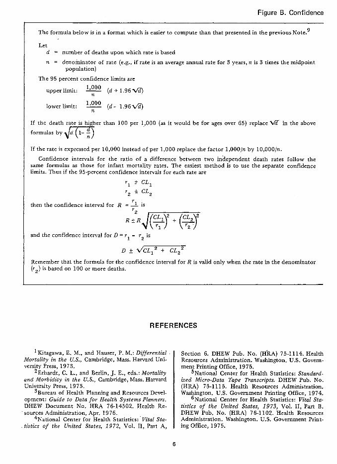
Figure B. Confidence

The formula below is in a format which is easier to compute than that presented in the previous Note.g

Let d = number of deaths upon which rate is based

~ = denominator of rate (e.g., if rate is an averageannu~ ratefor 3 yeas, n.is .3times the midpoint population)

The 95 percent confidence limits are

upper limit: ~ (d+l.96%@

lower limit: ~ (d- 1.96~

If the death rate is higher than 100 per 1,,000 (as it would be for ages over 65) replace ~ in the above

formulasbym If the rate is expressed per 10,000 instead of per 1,000 replace the factor 1,000/n by 10,000/n,

Confidence intervals for the ratio of a difference between two independent death rates follow the same formulas as those for infant mortality rates. The easiest method is to use the separate confidence limits. Thus if the 95-percent confidence intervals for each rate are

* CL2‘2

r 1 isthen the confidence interval for R —

and the confidence interval for D = r. - r- is

Remember that the formula for the confidence interval for R is valid only when the rate in the denominator (r2) is based on 100 or more deaths.

REFERENCES

1Kitagawa, E. M., and Hauser, P. M.: Differential I Section 6. DHEW Pub. No. (H-RA) 75-1114. Health Mortality in the U.S., Cambridge, Mass. Harvard Uni­versity Press, 1973.

2Erhardt, C. L., and Berlin, J. E., eds.: Mortality and Morbidity in the U.S., Cambridge, Mass. Harvard University Press, 1973.

3Bureau of Health Planning and Resources Devel­opment: Guide to Data for Health Systems Planners. DHEW Document No. HRA 76-14502. Health Re-sources Administration, Apr. 1976.

4National Center for Health Statistics:” Vital Sta­tistics of the United States, 1972, Vol. II, Part A,

Resources Administration. W&hingkm. U.S. Govern­ment Printing Office, 1975.

5National Center for Health Statistics: Standard­ized Micro-Data Tape Transcri@s. DHEW Pub. No. (HRA) 75-1115. Health Resources Administration. Washington. U.S. Government Printing Office, 1974.

6National Center for Health Statistics: Vital Sta­tistics of the United States, 1973, Vol. II, Part B. DHEW Pub. No. (HRA) 76-1102. Health Resources Administration. Washington. U.S. Government Print­ing Office, 1975.

6

intervals for death rates

The following data are based on deaths of white males aged 45-54 years andpopuIation for two U.S. counties (see tabIe I in appendix):

Santa Cruz, Calif. DeKalb, Ga.

Population (n) . 6,051 20,201 Number of deaths (dj : : : : : 63 155

Death rate +Xl,ooo . . . . 10.41 7.67 ( )

The 95-percent confidence intervals for the counties are

Santa Crw: - (63L 1.96@3) = .1653 (63& 15.5570)= 10.41 k2.57 9 Interwd: (7.84, 12.98)

DeKalb: - (155 &l.96~5) = .0495 (155~ 24.4018)= 7.67t 1.21 , Interval: (6.46, 8.88)

The confidence intervals for the ratio and difference are ~ = 10.41

Ratio: —= 1.367.67

L36~,.36~~ = L36tl.36ti0609+ .0249 =

1.36 t 1.36- = 1.36 ~ 1.36 (.2930) = 1.36 ~ .40 Interval: (0.96, 1.76)

Difference D = 10.41-7.67 = 2.74

2.74 iV!2.572 + 1.212 = 2.74L _ = 2.74 L2.84 Interval: (-0.10, 5.58)

Since the interval for D includes zero (or the interval for R includes 1) the rates for the two counties are not significantly different.

7Bureau of Health Planning and Resources Devel­opment, Health Resources Administration, and U.S. Bureau of the Census, Guide to Local Area Popula­tion Projection. (In press.)

8h’ational Center for Health Statistics: Compari­son of place of residence on death certificates and matching census records, United States, May-Aug. 1960. Vitat and Health Statistics. PHS Pub. No. 1000-Series 2-No. 30. Public Health Service. Washing-ton. U.S. Government Printing Office, Jan. 1969.

‘Sauer, H. I., et al.: Cardiovascular disease mor­tality patterns in Georgia and North Carolina. PzJb. Health Rep. 81:455-465, May 1966.

1‘National Center for Health Statistics: Infant mortality, by J. C. Kleinman. Statistical Notes for Health Planners, No. 2. Health Resources Administra­tion. Washington, D. C., JuIy 1976.

11 Kitagawa, E. M.: Theoretical consideration in the selection of a mortality index, and some empirical comparisons. Hum. BioL 38;293-308, Sept. 1966.

12 \vooIsey, T. D.: Adjusted death rates and other indices of mortality. Vital Statistics Rates in the U. S., 1900-1940, Chapter IV. U.S. Bureau of the Census. Washington. U.S. Government Printing Office, 1943. ,

13Kleinman, J. C.: A new look at mortality in­dexes with emphasis on small area estimation. Proc­eedings of the A nzerican Statistical Association, So­cial Statistics Section. 1976, (In press.)

14Haenszel, W.: A standardized rate for mortality in units of lost years of life. Am. J. Public Health. 40:17-26, Jan. 1950.

7

APPENDIX

AGE-ADJUSTED MORTALITY lNDEXESb —

We have seen (figure A) that the crude death rate is not a useful measure for com­paring mortality among areas or monitoring changes over time because it depends upon the population composition as well as the spe­cific death rates. Since there are such a large number of specific death rates which can be computed it is useful to summarize those rates in an overall mortality index which takes into acount different population composi­tions. These indexes are usually called age-adjusted or standardized death rates. Three in­dexes will be presented in this note. For a more complete discussion see Kitagawal 1 and Woolsey.l Z The indexes will be explained in reference to age-adjustment. A future note will discuss more general adjusted rates.

Table I shows the age-specific death rates for white males in two U.S. counties. These counties will be used to illustrate the adjust­ment procedures. Note that the death rate for Santa Cruz males ( 15.62) is over twice as high as the rate for DeKalb males (6.58). The dif­ference in overall death rates is greatly in­fluenced by the age distributions–nearly 15 percent of Santa Cruz’s white males are 65 or over compared to only 4 percent of DeKalb’s white males.

Examination of the age-specific death rates shows that DeKalb has substantially lower rates in the,l 5-54 age groups and slight­ly higher rates in the older age groups (figure I). If a single measure is used to summarize the age-specific rates, it will not reflect this “crossover” in the curves (see figure I). When-ever such a crossover is present, the indexes presented here should be used with caution. In a later section we discuss the use of the indexes over narrower age ranges. When plot­ting death rates which vary widely (as they do over the entire age range) it is convenient to use a logarithmic scale.

The following notation will be used in the discussion (for a particular race-sex group):

bThis is a more indepth discussion of age-adjusted rates than that presented in the Census Guide3 (which included only the direct method of adjustment).

pa = area population in age group a

p=~pa= total population

da = number of deaths in area for age a

d = Zda = total number of deaths in area

_d -L x 1,000 = area’s age-specific death rate

“- Pa per 1,000

Note that the race-sex specific death rate can be written as

Pa RSDR = d X 1,000 = Zma — (1)

F P

This was illustrated in figure 1 ; the area’s death rate is a weighted average of age-specific rates using the area’s age distribution as weights.

Indirect Method

The indirect method of adjustment corn- – pares the area’s death rate with an “expected” death rate based on the area’s population composition and a standard set of rates. The method will be illustrated for white males us­ing U.S. rates as the standard. If the area’s age-specific rates for white males were ex­actly the same as the U.S. age-specific rates for white males, the expected number of white male deaths in age group a would be the product of the U.S. rate and the number of white males in age group a in the area divided by 1,000:

1 — 1,000 Mapa

where the Ma is the U.S. age-race-sex specific rate per 1,000. Thus the total number of ex­pected deaths for white males is just the sum of these products over all age groups:

& ~Mapa )

The standardized mortality ratio (SMR) is

—. 8

Table 1. White male death rates for two U.S. counties, 1970

Santa Cruz, California

I Years

Expected Age

Population Numberof Death

of life Expected years

deaths rates lost deaths of life IOst

(1) (2) (3) (4) (5) (6) (7)I I

Total . . . . . . . . . . . . . . . . 56,478 I 882 I 15.62 6,480 884.18 5,893.0

Under l year . . . . . . . . . . . . . . . . . . . 847 16 18.89 1,112 17.80 1,244.1 l-4 years . . . . . . . . . . . . . . . . . . . . . . 3,274 4 1.22 268 2.75 184.3 5-14years . . . . . . . . . . . . . . . . . . . . 10,279 3 0.29 180 4.93 285.8 15-24years . . . . . . . . . . . . . . . . . . . . 10,201 24 2.35 1,200 17.44 872.0 25-34 years . . . . . . . . . . . . . . . . . . . . 6,413 14 2.18 560 11.35 454.0 3544 years . . . . . . . . . . . . . . . . . . . . 5,661 26 4.59 780 19.47 584.1 45-54 years . . . . . . . . . . . . . . . . . . . 6,051 63 10.41 1,260 53.43 1,068.6 55-64 years . . . . . . . . . . . . . . . . . . . . 5,402 112 20.73 1,120 119,01 1,190.1 65-74 years . . . . . . . . . . . . . . . . . . . . 4,920 225 45.73 236.65 75a4 years . . . . . . . . . . . . . . . . . . . . 2,781 275 98.89 ... 280.85 ... 85 yearsand over, ...,..... . . . . . 649 120 164.90 ... 120.40 ...

DaKalb, Georgia

Years Expected

Age Population

Numberof Death of life

Expected years deaths rates deaths of life

lost IOst

(1) (2) (3) (4} (5) (6) (7)

Total . . . . . . . . . . . . . . . . . 173,051 1,139 6.58 16,712 1,190.66 19,635.4

Under l year . . . . . . . . . . . . . . . . . . 3,325 64 19.25 4,448 70.26 4,883.1 1~ years . . . . . . . . . . . . . . . . . . . . . 12,669 12 0.95 804 10.64 712.9 5-14years . . . . . . . . . . . . . . . . . . . . . 37,883 13 0.34 780 18.18 1,090.8 15-24 years . . . . . . . . . . . . . . . . . . . . 29,136 31 1.06 1,550 49.82 2,491.0 25-34 years . . . . . . . . . . . . . . ,..,,, 27,383 41 1.50 1,640 48.47 1,938.8 3544 years . . . . . . . . . . . . . . . . . . . 24,223 68 2.81 2,040 83.33 2,499.9 45-54 years . . . . . . . . . . . . . . . . . . . . 20,201 155 7.67 3,100 178.37 3,567.4 55-64 years . . . . . . . . . . . . . . . . . . . . 11,128 235 21.12 2,350 245.15 2,451.5 65-74 years . . . . . . . . . . . . . . . . . . . . 4,901 252 51.42 . .. 235.74 . ..

75-84years . . . . . . . . . . . . . . . . . . . . 1,867 199 106.59 . .. 188.55 ...

85 years and over . . . . . . . . . . . . . . . 335 69 205.97 ... 62.15 ...

then defined as a ratio of observed to ex- 1 da. —

1,;00 ‘J”pected numberof deaths: I theSMRcanbe writtenas

By using some algebra we can express the Thus the SMR is also a ratio of the area’s SMR as a ratio of rates. Since I observed death rateto its expected death rate.

— 9

Figure 1. Age-specific death rates for white males in two U.S. counties, 1970

300

200

F

100 — 90 — 80 — 70 —

60 —

50 —

40 —

30 —

20 —

To — 9 — 8 — 7 —

6 “

5 —

4 —

3* —

2 —

1 .9 — .a — .7 —

.6 —

.5 —

.4 —

.3 —

Santa Cruz

DeKalb 4

. . . . . . .

�

�

�* �’

b

i

300

200

100 90 80 70 60

50

40

30

20

10 9 8

7

6

5

4

3

2

1 — .9 — .8

.7

— .6

— .5

— .4

— .3

.2 I I I I o 10’

.2 20 30 40 50 60 70 80 90

AGE IN YEARS

10

Table II. U.S. population distribution and age-specific death rates, 1970

Death rates per 1,000 Proportion (F’a/P)

Age of United States population- White White Other Other

male female male female

Underl year .... . .. .... .. . .. ... . ..... .. ... .. . .. .. .... . ... .. .. 14 years ... .. .. .. .. .. .. ... .. .. ... .. . ... . ... .... . .. ... .. .. .. .. . . . 5-14 years . . ... .... . ... ... . .. .... . .. ... .. . ..... .. .... .. . .... . .. . 15-24 years .. .... .. .. .... .. . ... .. .. .... . .. ... . .. ... .. .. .... . . .. 25-34 years .. .... .. .. .... ... .... . . ... .. . .... ... .. .. .. . .... . .. .. 35-44 years .. .... . ... .. .. .. .. .. ... ... . .. ... ... . .... . .. .... .. ... 45-54 years ..... . ... .... . . .... ..o. ... .. . .... .. .... . ... ... .. .. .. 55-64 years .... .. .. ... ... .. ... .. .. .. ... .... .. .. ... .. .. .. .. .. ... 65-74 years ..... . . ..... . . .... . .. ... .... ..... .. ... . ... .... .. . ... 75-84 years ... .. .. .... .. . .... . ... .. .... ... .. .. ... .. . .... .. .. .. . 85 years and over .. .. .... .. .. ... .. . ... ... . .... . . .... . .. ... .

The absolute value of the SillR is in­fluenced by the standard set of rates Ma. However, since the purpose of the SNIR is to compare areas, it is the reIative values of the SMR’S which are important. Choosing the standard as the set of U.S. rates for the pe­riod under study is recommended since that will allow comparison of areas between and within different States or HSA’S. These rates are shown in tabIe II for 1970.

For the two counties in table I, the ex­pected numbers of deaths are shown in col­umn (6).

Thus the ShfR’s are

Santa Cruz: SMR~ = - = .998

DeKalb: SMR~ = 1’139 = .957 1,190.66

Note that these indexes are much cIoser than the crude rates.

A combined SMR for all races and both sexes is often used instead of the individual race and sex-specific SMR’S. In this case, the observed and expected number of deaths are each summed over all race-sex groups and a single ratio obtained. The problem with doing this is that there may be problems specific to a race-sex group which will not show up in the combined index. Indeed, for U.S. counties in 1969-71 there were substantial differences among the race-sex specific ShfR’s. 13

.0172 21.13 16.15 40.20 31.69

.0673 .84 .66 1.45 1.23

.2005 .48 .30 .65 .42

.1744 1.71 .62 3.05 1.08

.1226 1.77 .84 5.04 2.16

.1136 3.44 1.93 8.74 4.91

.1143 8.83 4.63 16.46 9.79

.0915 22.03 10.15 30.47 18.87

.0612 48.10 24.71 54,74 36.76

.0301 100.99 66.99 89.81 63.93

.0074 185.52 159.80 114.05 102.89

Direct Method

Another procedure for age adjustment is the direct method. In the direct method a standard age distribution is chosen and the area’s age-specific death rat es are weighted ac­cording to the standard. A reasonable choice for the standard is the U.S. total population (ail races, both sexes) for the year under study or the average population of the areas under study. If time trends are being ana­lyzed, the population for the most recent de­cennial census year can be used.

The direct age-adjusted rate is

DAR = Em ~ aP

where Pa = standard population in age group a and

P = zPa

(The values of Pa/P for the U.S. 1970 popula­tion are shown in table H.) By comparing this expression with (1), it is seen that the only difference between the race-specific death rate (RSDR) and the direct age-adjusted rate (DAR) is the weights which are applied to the age-specific rates.

For the two counties in figure I

Santa Cruz: DAR~ = 18.89 x.0172 + 1.22 x .0673 + . . . + 184.90 X .0074 = 11.90

DeKalb: DAR~ = 19.25 x.0673 + . . . + 205.97 x .0074 = 11.85

11

Thus the two direct age-adjusted rates are very similar, like the SMR’S.

It is important to remember that the di­rect age-adjusted rate is a death rate for a hypothetical . population. Its absolute value has little meaning. To keep this point in mind it is best to express the DAR as a ratio to the U.S. death rate for the appropriate race-sex group. Thus we define the comparative mortal­ity figure CMF as

(3)

where Ma is the race-sex-specific death rate for age group a. For example, for white males the denominator is

21.13 x.0172 +.84 x.0673 +.. .+185.52x.0074 = 11.80

Thus the CMF’S for the two counties are

Santa Cruz: CMF~ = ~ = 1.008 11.80

11.85DeKalb: — = 1.004

“UFD = 11.80

The difference between the counties in CMF’S is smaller than the difference in ShlR’s, since the CMF uses the same set of weights for each county while the SMR uses each county’s population. Thus if the counties had exactly the same set of age-specific death rates their CMF’S would be equal (unlike the situation with respect to the SMR). Com­paring formulas (2) and (3) reveals that the only difference is the weights applied.

Comparison of t;e Indexes

It has already been pointed out that the different age distributions used in the SMR makes two SMR’S less comparable than two CMF’S. However, there are two reasons for using the SMR as it stands:

(1) Data availability. –The SMR requires only the total number of deaths in an area for each race-sex group with no need to calculate all the age-specific rates. This is a special advantage when the only data available are published county or area totals.

(2) Public Health implications. –By weighting according to the area’s age distribution, the SMR emphasizes the rates as they apply to the area’s popu­lation. Thus a high rate combined with high population concentration is emphasized. This property makes the indirect method more appropriate for planning applications.

A disadvantage which is shared by the CMF and the SMR is an emphasis on death rates in the elderly. For example, suppose the death rate in the 85 or over group doubles. The number of deaths in this group also doubles and the two indexes for Santa Cruz become

SMR~ = 1.133, a 13.5-percent increase over original SMR~

CMF~ = 1.124, a 11.6-percent increase over original CMF~

However, if the death rate for the 15-24 group doubles the indexes become

SMR~ = 1.025, a 2.7-percent increase over original SMR~

CMF~ = 1.043,a 3.5-percent increase over original CMF=

Thus an increase in rate for the young age group has little effect on the CMF or SMR since the number of deaths involved is small while the opposite is true for an increase in rate among the elderly. This is why the SMR and CMF were nearly equal for the two counties despite the differences in the death rates for ages 15-44. For use in planning, the emphasis on the elderly is unfortunate since mortality in this group is probably least amen-able to planning intervention (the opposite might well be true for morbidity or disability).

Years of Life Lost

One method for emphasizing mortality in the younger age groups is to express deaths in terms of years of life lost rather than numbers of deaths. 14 An easy method for doing this is to assume that each individual has 70 “pro­ductive” years of life and so a death at age a results in 7 O-a years of life lost when a< 70. When using the 11 age groups, all deaths are assumed to occur at the midpoint of the in-

12

terval. Since the midpoint of the 65-74 inter­val is 70, all deaths in this group and the two older groups are omitted from the computa­tion of years of life lost. For exampIe, the numbers of years of life lost in the two coun­ties (column 5 of table I) are:

SantaCruz: 16x69 .5+4x 67+3x 60+. .. +112x 10 = 6480

DeKalb: 64x69 .5+12 x67+13 x60+. .. +235 X 10= 16712

In order to use years of life lost in an index we need to adjust for different age dis­tributions as we did previously. We can use either a direct or indirect approach which have the same advantages and disadvantages discussed above. For ease of calculation and public health implications we choose the in-direct method. As we did for the SMR, we calculate an expected number of deaths for each age group. But instead of adding these up we first translate expected deaths into ex­pected years of life lost by multiplying ex­pected deaths by 70 minus the midpoint of the age interval. The expected years of life lost for the two counties are given in column 7 of table I:

SantaCruz: 17.90 x69.5 +2.75 x67 +4.93 x60 + . . . + 119.01 X 10= 5,893.0

De&Jb: 70.26X69.5 +1 O.64X67+18.18X6O + . . . + 245.15 x 10= 19,635.4

The years of life lost (YLL) index for each county is the ratio of observed to ex­pected years of life lost:

6480SantaCruz: YLL~ = - = 1.100

5,893.0

DeKalb: YLLD = 16’712 = 0.851 19,635.4

In this case, Santa Cruz, with its higher death rates in the young age groups, does show a moderately higher YLL index than DeKalb.

The fo;md-a for YLL is:

YLL = Xia (70-Ya) ~%Pa (70-Ya)

= Z&Iapa (70 - ya)J-1,000

m’fapa (70-Ya)

where y-, is the midpoint of the age interval and the sum extends only to the 55-64 age group:

The YLL index, unlike the SMR and ChlF, emphasizes the differences in age-specific mortality at younger ages. This can be illustrated by the effect of doubling the death rate for the 15-24 age group in Santa Cruz. The number of deaths in this group will in-crease from 24 to 48 and the corresponding years of life lost will increase to 2400. The total observed years of life lost becomes 7680 and the YLL index is

YLL=~= 1.3035,893.0

This represents an 18.5 percent increase over the original YLL (compare this to the 3-4 per-cent increases in ShfR and CMF given earlier).

A detailed comparison of’ these firee in­dexes ,.is presented in the reference. 13 For health planners, the years of life lost index seems most appropriate.

Confidence Intervals for Mortality Indexes

The confidence intervals for the indexes discussed previously are obtained by the for­mulas in figure II. These formulas are similar to the ones used to compute the indexes and so the additional computations are not time-consuming. Note that the confidence interval for YLL is wider than the intervals for the ChIF and ShlR. This is because the YLL em­phasizes death rates for younger age groups and these death rates generally have larger random &-ror than those based on large num­ber of deaths (as in the older age groups). Thus aggregation over years will usually be required even when dealing with these sum­mary indexes. If 3 years of data are com­bined, the YLL is reasonably stable for popu­lations of 10,000 or more. 13

When comparing the same index for dif­ferent areas, the ratio of the two indexes should be used. Figure III shows the formulas for computing 95-percent confidence intervals for the ratio. If the interwd does not include a ratio of one, the indexes are significantly dif­ferent at the 5-percent level. In order for the formula to be used, the indexes must be inde­pendent, i.e., no death included in one index can be included in the other. In addition, the index in the denominator should be based on at least 100 deaths.

13

Figure II. Confidence intervals for mortality indexes

The confidence interval for one of the indexes discussed is approximated

by 1 f 1.96s1 (1) where 1 = index

SI = standard error of the index

The standard error of each index is approximately:

G ‘sMR = 1

—~MaPa 1,000

,CMF=J­

~Ma+

SYLL = ~Z da (70-ya)2

& ~MaPa (70 -y,) ,

Using the data from table I, the following standard errors are obtained”:

Santa Cruz, C%lif. DeKalb, Ga.

.0336 .0283 ‘SMR ””””’”

‘CM F””””””,0349 .0330 .0845 .0426

‘YLL . . . . . .

Confidence intervals are obtained using formula (1):

Santa Cruz, Califi

SMR . . . . . . (.932, 1.064) CMF . . . . . . (.940, 1.076) YLL . . . . . . (.934, 1.266)

Use of Indexes for Portions of the Age Range

We have seen in figure I that there is a crossover in the age-specific death rates be-tween Santa Cruz and DeKalb, i.e., for the younger age groups DeKalb has lower death rates, but for the older age groups DeKalb has higher rates. A single measure of mortality cannot reflect such differences. Yet examina­tion of all the age-specific rates for more than two areas is very difficult and is subject to the vagaries of random error in the rates (see sec­tion in text, “StabiIity”). A compromise be-tween a single measure and all eleven age-specific rates is to compute indexes for por­tions of the age range. A general strategy might be to examine the infant mortality rate separately (using live births as the den,ornina-

DeKalb, Ga.

(.902, 1.01 2) (.939, 1.069) (.768, ,934)

torg ), then use SMR’S for the age ranges 1-34, 35-64, and 65 and eve;. The SMR’S for the narrow age groups are obtained as before ex­cept that only observed and expected deaths for the relevant age groups are used. For ex­ampIe, the SMR for aged 1-34 in Santa Cruz is

4+3+24+14SMR1-34 =

2.75+4.93+17.44+11.35

45 -—= 1.234 ‘36.47

The YLL index could also be used for the age groups under 65 (or even in the group 65 and over by modifying the ‘.’expected” years from 70 to, say, 95). However, over the narrower age ranges the differences bet ween the YLL and the SMR should be small (e.g., YLL1-34 for Santa Cruz is 1.223).

14

Figure I I 1. Confidence interval for the ratio of independent indexes

Let II = mortality index for area 1 ~1,= standard error of 11 1

12 = mortality index for area 2

S12= standard error of 12

The confidence limits for R are

upper limit: R + 1.96R /--7

lower limit: R -1’6RJWW

For example, using the YLL’s for Santa Cruz, Calif. and DeKalb, Ga.

YLL~ = 1.100 = .0845‘YLL~

YLL ~ = 0.851 ‘YLLD = .0426

R = 1.293

,96 R~~=2.~~d X .0917 = .232

R + .232 = 1.525

R - .232 = 1.061

Thus the years of life lost index is from 6 percent to 53 percent higher in Santa Cruz, Calif. than in DeKalb, Ga. Since the interval does not include 1, the two indexes are significantly different at the 5-percent level.

The confidence interval for the ratio can also be obtained directly from the confidence interval for each index. Suppose these intervals are

11 L (7Ll

12 & CL2

11 Then the confidence interval for R = y is

2

I “Rm These formulas should only be used when the index in the denominator is based upon more than 100

deaths.

15

GPO 914.570

The SMR’S for each county are given be-low: I

Age San ta Cruz DeKalb I

1-34 years . . . . 1.234 0.763 35-64 years . . . . 1.04’7 0.904

65 years and over . . 0.972 1.069

These SMR’S give a clearer picture of the dif­ferences between the two counties: Santa Cruz has much higher death rates in the young age groups, somewhat higher rates in middle age, and somewhat lower rates among the elderly.

Standard errors and confidence intervals are computed as before {figure H) except that the summation extends over only those age groups included in the index. For example, the standard error of the SMR for aged 1-34 in Santa Cruz is

SE.& =.184

Statistical Notes for Health Planners is a cooperative activity of the National Center for Hea\th Statistics and the Bureau of Health Planning and Resources Develop­ment, Health Resources Administration.

Information, questions, and contributions should be directed to Mary Grace Kovar, Division of Analysis, NCHS, Room 8A-55, Parklawn Building, 5600 Fishers Lane, Rockville, Md. 20857.

16