statistical natural language processing - nyu

199

CHAPTER 4

Statistical Natural Language

Processing

4.0 Introduction . . . . . . . . . . . . . . . . . . . . . . . . . . . . . 1994.1 Preliminaries . . . . . . . . . . . . . . . . . . . . . . . . . . . . . 2004.2 Algorithms . . . . . . . . . . . . . . . . . . . . . . . . . . . . . . 201

4.2.1 Composition . . . . . . . . . . . . . . . . . . . . . . . . . 2014.2.2 Determinization . . . . . . . . . . . . . . . . . . . . . . . 2064.2.3 Weight pushing . . . . . . . . . . . . . . . . . . . . . . . 2094.2.4 Minimization . . . . . . . . . . . . . . . . . . . . . . . . 211

4.3 Application to speech recognition . . . . . . . . . . . . . . . . . 2134.3.1 Statistical formulation . . . . . . . . . . . . . . . . . . . 2144.3.2 Statistical grammar . . . . . . . . . . . . . . . . . . . . . 2154.3.3 Pronunciation model . . . . . . . . . . . . . . . . . . . . 2174.3.4 Context-dependency transduction . . . . . . . . . . . . . 2184.3.5 Acoustic model . . . . . . . . . . . . . . . . . . . . . . . 2194.3.6 Combination and search . . . . . . . . . . . . . . . . . . 2204.3.7 Optimizations . . . . . . . . . . . . . . . . . . . . . . . . 222Notes . . . . . . . . . . . . . . . . . . . . . . . . . . . . . . . . . 225

4.0. Introduction

The application of statistical methods to natural language processing has beenremarkably successful over the past two decades. The wide availability of textand speech corpora has played a critical role in their success since, as for alllearning techniques, these methods heavily rely on data. Many of the compo-nents of complex natural language processing systems, e.g., text normalizers,morphological or phonological analyzers, part-of-speech taggers, grammars orlanguage models, pronunciation models, context-dependency models, acousticHidden-Markov Models (HMMs), are statistical models derived from large datasets using modern learning techniques. These models are often given as weighted

automata or weighted finite-state transducers either directly or as a result of theapproximation of more complex models.

Weighted automata and transducers are the finite automata and finite-state

Version June 23, 2004

200 Statistical Natural Language Processing

Semiring Set ⊕ ⊗ 0 1

Boolean {0, 1} ∨ ∧ 0 1Probability R+ + × 0 1Log R ∪ {−∞, +∞} ⊕log + +∞ 0Tropical R ∪ {−∞, +∞} min + +∞ 0

Table 4.1. Semiring examples. ⊕log is defined by: x ⊕log y = − log(e−x + e−y).

transducers described in Chapter 1 Section 1.5 with the addition of some weightto each transition. Thus, weighted finite-state transducers are automata inwhich each transition, in addition to its usual input label, is augmented withan output label from a possibly different alphabet, and carries some weight. Theweights may correspond to probabilities or log-likelihoods or they may be someother costs used to rank alternatives. More generally, as we shall see in the nextsection, they are elements of a semiring set. Transducers can be used to definea mapping between two different types of information sources, e.g., word andphoneme sequences. The weights are crucial to model the uncertainty of suchmappings. Weighted transducers can be used for example to assign differentpronunciations to the same word but with different ranks or probabilities.

Novel algorithms are needed to combine and optimize large statistical modelsrepresented as weighted automata or transducers. This chapter reviews severalrecent weighted transducer algorithms, including composition of weighted trans-ducers, determinization of weighted automata and minimization of weightedautomata, which play a crucial role in the construction of modern statisticalnatural language processing systems. It also outlines their use in the designof modern real-time speech recognition systems. It discusses and illustratesthe representation by weighted automata and transducers of the components ofthese systems, and describes the use of these algorithms for combining, search-ing, and optimizing large component transducers of several million transitionsfor creating real-time speech recognition systems.

4.1. Preliminaries

This section introduces the definitions and notation used in the following.A system (K,⊕,⊗, 0, 1) is a semiring if (K,⊕, 0) is a commutative monoid

with identity element 0, (K,⊗, 1) is a monoid with identity element 1, ⊗ dis-tributes over ⊕, and 0 is an annihilator for ⊗: for all a ∈ K, a⊗ 0 = 0⊗ a = 0.Thus, a semiring is a ring that may lack negation. Table 4.1 lists some familiarsemirings. In addition to the Boolean semiring, and the probability semiringused to combine probabilities, two semirings often used in text and speech pro-cessing applications are the log semiring which is isomorphic to the probabilitysemiring via the negative-log morphism, and the tropical semiring which is de-rived from the log semiring using the Viterbi approximation. A left semiring isa system that verifies all the axioms of a semiring except from the right ditribu-tivity. In the following definitions, K will be used to denote a left semiring or a


4.2. Algorithms 201

semiring.A semiring is said to be commutative when the multiplicative operation ⊗

is commutative. It is said to be left divisible if for any x 6= 0, there existsy ∈ K such that y ⊗ x = 1, that is if all elements of K admit a left inverse.(K,⊕,⊗, 0, 1) is said to be weakly left divisible if for any x and y in K such thatx⊕y 6= 0, there exists at least one z such that x = (x⊕y)⊗z. The ⊗-operationis cancellative if z is unique and we can write: z = (x ⊕ y)−1x. When z is notunique, we can still assume that we have an algorithm to find one of the possiblez and call it (x ⊕ y)−1x. Furthermore, we will assume that z can be found ina consistent way, that is: ((u ⊗ x) ⊕ (u ⊗ y))−1(u ⊗ x) = (x ⊕ y)−1x for anyx, y, u ∈ K such that u 6= 0. A semiring is zero-sum-free if for any x and y in K,x⊕ y = 0 implies x = y = 0.

A weighted finite-state transducer T over a semiring K is an 8-tuple T =(A,B, Q, I, F, E, λ, ρ) where: A is the finite input alphabet of the transducer; Bis the finite output alphabet; Q is a finite set of states; I ⊆ Q the set of initialstates; F ⊆ Q the set of final states; E ⊆ Q×(A∪{ε})×(B∪{ε})×K×Q a finiteset of transitions; λ : I → K the initial weight function; and ρ : F → K the finalweight function mapping F to K. E[q] denotes the set of transitions leaving astate q ∈ Q. |T| denotes the sum of the number of states and transitions of T.

Weighted automata are defined in a similar way by simply omitting the inputor output labels. Let Π1(T) (Π2(T)) denote the weighted automaton obtainedfrom a weighted transducer T by omitting the input (resp. output) labels of T.

Given a transition e ∈ E, let p[e] denote its origin or previous state, n[e]its destination state or next state, i[e] its input label, o[e] its output label,and w[e] its weight. A path π = e1 · · · ek is an element of E∗ with consecutivetransitions: n[ei−1] = p[ei], i = 2, . . . , k. n, p, and w can be extended topaths by setting: n[π] = n[ek] and p[π] = p[e1] and by defining the weight ofa path as the ⊗-product of the weights of its constituent transitions: w[π] =w[e1] ⊗ · · · ⊗ w[ek]. More generally, w is extended to any finite set of paths Rby setting: w[R] =

⊕

π∈R w[π]. Let P (q, q′) denote the set of paths from q toq′ and P (q, x, y, q′) the set of paths from q to q′ with input label x ∈ A∗ andoutput label y ∈ B∗. These definitions can be extended to subsets R, R′ ⊆ Q,by: P (R, x, y, R′) = ∪q∈R, q′∈R′P (q, x, y, q′). A transducer T is regulated if theweight associated by T to any pair of input-output string (x, y) given by:

[[T]](x, y) =⊕

π∈P (I,x,y,F )

λ[p[π]]⊗ w[π] ⊗ ρ[n[π]] (4.1.1)

is well-defined and in K. [[T]](x, y) = 0 when P (I, x, y, F ) = ∅. In particular,when it does not have any ε-cycle, T is always regulated.

4.2. Algorithms

4.2.1. Composition

Composition is a fundamental algorithm used to create complex weighted trans-ducers from simpler ones. It is a generalization of the composition algorithm



presented in Chapter 1 Section 1.5 for unweighted finite-state transducers. LetK be a commutative semiring and let T1 and T2 be two weighted transducersdefined over K such that the input alphabet of T2 coincides with the output al-phabet of T1. Assume that the infinite sum

⊕

z T1(x, z)⊗T2(z, y) is well-definedand in K for all (x, y) ∈ A∗×C∗. This condition holds for all transducers definedover a closed semiring such as the Boolean semiring and the tropical semiringand for all acyclic transducers defined over an arbitrary semiring. Then, theresult of the composition of T1 and T2 is a weighted transducer denoted byT1 ◦ T2 and defined for all x, y by:

[[T1 ◦ T2]](x, y) =⊕

z

T1(x, z)⊗ T2(z, y) (4.2.1)

Note that we use a matrix notation for the definition of composition as opposedto a functional notation. There exists a general and efficient composition al-gorithm for weighted transducers. States in the composition T1 ◦ T2 of twoweighted transducers T1 and T2 are identified with pairs of a state of T1 anda state of T2. Leaving aside transitions with ε inputs or outputs, the followingrule specifies how to compute a transition of T1◦T2 from appropriate transitionsof T1 and T2:

(q1, a, b, w1, q2) and (q′1, b, c, w2, q′2) =⇒ ((q1, q

′1), a, c, w1 ⊗ w2, (q2, q

′2)) (4.2.2)

The following is the pseudocode of the algorithm in the ε-free case.

Weighted-Composition(T1, T2)

1 Q← I1 × I2

2 S ← I1 × I2

3 while S 6= ∅ do

4 (q1, q2)← Head(S)5 Dequeue(S)6 if (q1, q2) ∈ I1 × I2 then

7 I ← I ∪ {(q1, q2)}8 λ(q1, q2)← λ1(q1)⊗ λ2(q2)9 if (q1, q2) ∈ F1 × F2 then

10 F ← F ∪ {(q1, q2)}11 ρ(q1, q2)← ρ1(q1)⊗ ρ2(q2)12 for each (e1, e2) ∈ E[q1]× E[q2] such that o[e1] = i[e2] do

13 if (n[e1], n[e2]) 6∈ Q then

14 Q← Q ∪ {(n[e1], n[e2])}15 Enqueue(S, (n[e1], n[e2]))16 E ← E ∪ {((q1, q2), i[e1], o[e2], w[e1]⊗ w[e2], (n[e1], n[e2]))}17 return T

The algorithm takes as input T1 = (A,B, Q1, I1, F1, E1, λ1, ρ1) and T2 =(B, C, Q2, I2, F2, E2, λ2, ρ2), two weighted transducers, and outputs a weighted


4.2. Algorithms 203

0 1

2

3/0.7

a:b/0.1

a:b/0.2

b:b/0.3

b:b/0.4

a:b/0.5

a:a/0.6

0 1

2

3/0.6b:b/0.1

b:a/0.2

a:b/0.3

a:b/0.4

b:a/0.5

(a) (b)

(0,0) (1,1)

(0,1)

(2,1) (3,1)

(3,2)

(3,3)/.42a:b/.01

a:a/.04

a:a/.02

b:a/.06

b:a/.08

a:a/.1

a:b/.18

a:b/.24

(c)

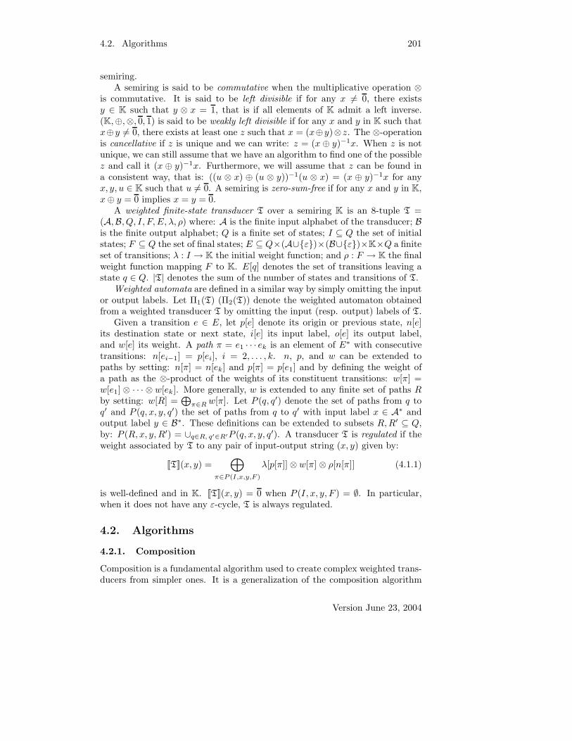
Figure 4.1. (a) Weighted transducer T1 over the probabilityl semiring.(b) Weighted transducer T2 over the probability semiring. (c) Composi-tion of T1 and T2. Initial states are represented by an incoming arrow,final states with an outgoing arrow. Inside each circle, the first numberindicates the state number, the second, at final states only, the value ofthe final weight function ρ at that state. Arrows represent transitions andare labeled with symbols followed by their corresponding weight.

transducer T = (A, C, Q, I, F, E, λ, ρ) realizing the composition of T1 and T2.E, I, and F are all assumed to be initialized to the empty set.

The algorithm uses a queue S containing the set of pairs of states yet tobe examined. The queue discipline of S can be arbitrarily chosen and doesnot affect the termination of the algorithm. The set of states Q is originallyreduced to the set of pairs of the initial states of the original transducers and Sis initialized to the same (lines 1-2). Each time through the loop of lines 3-16, anew pair of states (q1, q2) is extracted from S (lines 4-5). The initial weight of(q1, q2) is computed by ⊗-multiplying the initial weights of q1 and q2 when theyare both initial states (lines 6-8). Similar steps are followed for final states (lines9-11). Then, for each pair of matching transitions (e1, e2), a new transition iscreated according to the rules specified earlier (line 16). If the destination state(n[e1], n[e2]) has not been found before, it is added to Q and inserted in S (lines14-15).

In the worst case, all transitions of T1 leaving a state q1 match all thoseof T2 leaving state q′1, thus the space and time complexity of composition isquadratic: O(|T1||T2|). However, a lazy implementation of composition canbe used to construct just the part of the composed transducer that is needed.Figures 4.1(a)-(c) illustrate the algorithm when applied to the transducers ofFigures 4.1(a)-(b) defined over the probability semiring.

More care is needed when T1 admits output ε labels and T2 input ε labels.Indeed, as illustrated by Figure 4.2, a straightforward generalization of the ε-



(0,0) (1,1) (1,2)

(2,1)

(3,1)

(2,2)

(3,2)

(4,3)/1

a:d/1

(x:x)

ε:e/1

(ε1:ε1)

b:ε/1(ε2:ε2)

c:ε/1(ε2:ε2)

b:ε/1(ε2:ε2)

c:ε/1(ε2:ε2)

d:a/1(ε2:ε1)

ε:e/1

(ε1:ε1)

ε:e/1

(ε1:ε1)

b:e/1(ε2:ε1) 0 1 2 2 3/1

a:a/1 b:ε/1 c:ε/1 d:d/1

0 1 2 3/1a:d/1 ε:e/1 d:a/1

Figure 4.2. Redundant ε-paths. A straightforward generalization ofthe ε-free case could generate all the paths from (1, 1) to (3, 2) whencomposing the two simple transducers on the right-hand side.

free case would generate redundant ε-paths and, in the case of non-idempotentsemirings, would lead to an incorrect result. The weight of the matching pathsof the original transducers would be counted p times, where p is the number ofredundant paths in the result of composition.

To cope with this problem, all but one ε-path must be filtered out of the com-posite transducer. Figure 4.2 indicates in boldface one possible choice for thatpath, which in this case is the shortest. Remarkably, that filtering mechanismcan be encoded as a finite-state transducer.

Let T1 (T2) be the weighted transducer obtained from T1 (resp. T2) byreplacing the output (resp. input) ε labels with ε2 (resp. ε1), and let F be thefilter finite-state transducer represented in Figure 4.3. Then T1◦F◦T2 = T1◦T2.Since the two compositions in T1◦F◦T2 do not involve ε’s, the ε-free compositionalready described can be used to compute the resulting transducer.

Intersection (or Hadamard product) of weighted automata and compositionof finite-state transducers are both special cases of composition of weightedtransducers. Intersection corresponds to the case where input and output la-bels of transitions are identical and composition of unweighted transducers isobtained simply by omitting the weights.

In general, the definition of composition cannot be extended to the case ofnon-commutative semirings because the composite transduction cannot alwaysbe represented by a weighted finite-state transducer. Consider for example, thecase of two transducers T1 and T2 accepting the same set of strings (a, a)∗, with[[T1]](a, a) = x ∈ K and [[T2]](a, a) = y ∈ K and let τ be the composite of thetransductions corresponding to T1 and T2. Then, for any non-negative integern, τ(an, an) = xn ⊗ yn which in general is different from (x ⊗ y)n if x and y


4.2. Algorithms 205

0/1

1/1

2/1

x:x/1

ε2:ε1/1ε1:ε1/1

x:x/1

ε1:ε1/1

ε2:ε2/1

x:x/1

ε2:ε2/1

Figure 4.3. Filter for composition F.

do not commute. An argument similar to the classical Pumping lemma canthen be used to show that τ cannot be represented by a weighted finite-statetransducer.

When T1 and T2 are acyclic, composition can be extended to the case of non-commutative semirings. The algorithm would then consist of matching pathsof T1 and T2 directly rather than matching their constituent transitions. Thetermination of the algorithm is guaranteed by the fact that the number of pathsof T1 and T2 is finite. However, the time and space complexity of the algorithmis then exponential.

The weights of matching transitions and paths are ⊗-multiplied in composi-tion. One might wonder if another useful operation, ×, can be used instead of⊗, in particular when K is not commutative. The following proposition provesthat that cannot be.

Proposition 4.2.1. Let (K,×, e) be a monoid. Assume that × is used in-stead of ⊗ in composition. Then, × coincides with ⊗ and (K,⊕,⊗, 0, 1) is acommutative semiring.

Proof. Consider two sets of consecutive transitions of two paths: π1 =(p1, a, a, x, q1)(q1, b, b, y, r1) and π2 = (p2, a, a, u, q2)(q2, b, b, v, r2). Matchingthese transitions using × result in the following:

((p1, p2), a, a, x× u, (q1, q2)) and ((q1, q2), b, b, y × v, (r1, r2)) (4.2.3)

Since the weight of the path obtained by matching π1 and π2 must also corre-spond to the ×-multiplication of the weight of π1, x⊗ y, and the weight of π2,u⊗ v, we have:

(x× u)⊗ (y × v) = (x⊗ y)× (u⊗ v) (4.2.4)



This identity must hold for all x, y, u, v ∈ K. Setting u = y = e and v = 1 leadsto x = x ⊗ e and similarly x = e⊗ x for all x. Since the identity element of ⊗is unique, this proves that e = 1.

With u = y = 1, identity 4.2.4 can be rewritten as: x ⊗ v = x × v for all xand v, which shows that × coincides with ⊗. Finally, setting x = v = 1 givesu⊗ y = y × u for all y and u which shows that ⊗ is commutative.

4.2.2. Determinization

This section describes a generic determinization algorithm for weighted au-tomata. It is thus a generalization of the determinization algorithm for un-weighted finite automata. When combined with the (unweighted) determiniza-tion for finite-state transducers presented in Chapter 1 Section 1.5, it leads toan algorithm for determinizing weighted transducers.1

A weighted automaton is said to be deterministic or subsequential if it hasa unique initial state and if no two transitions leaving any state share the sameinput label. There exists a natural extension of the classical subset construc-tion to the case of weighted automata over a weakly left divisible left semiringcalled determinization.2 The algorithm is generic: it works with any weakly leftdivisible semiring. The pseudocode of the algorithm is given below with Q′, I ′,F ′, and E′ all initialized to the empty set.

Weighted-Determinization(A)

1 i′ ← {(i, λ(i)) : i ∈ I}2 λ′(i′)← 13 S ← {i′}4 while S 6= ∅ do

5 p′ ← Head(S)6 Dequeue(S)7 for each x ∈ i[E[Q[p′]]] do

8 w′ ←⊕

{v ⊗ w : (p, v) ∈ p′, (p, x, w, q) ∈ E}9 q′ ← {(q,

⊕{

w′−1 ⊗ (v ⊗ w) : (p, v) ∈ p′, (p, x, w, q) ∈ E}

) :q = n[e], i[e] = x, e ∈ E[Q[p′]]}

10 E′ ← E′ ∪ {(p′, x, w′, q′)}11 if q′ 6∈ Q′ then

12 Q′ ← Q′ ∪ {q′}13 if Q[q′] ∩ F 6= ∅ then

14 F ′ ← F ′ ∪ {q′}15 ρ′(q′)←

⊕

{v ⊗ ρ(q) : (q, v) ∈ q′, q ∈ F}16 Enqueue(S, q′)17 return T′

1In reality, the determinization of unweighted and that of weighted finite-state transducerscan both be viewed as special instances of the generic algorithm presented here but, for claritypurposes, we will not emphasize that view in what follows.

2We assume that the weighted automata considered are all such that for any string x ∈ A∗,w[P (I, x, Q)] 6= 0. This condition is always satisfied with trim machines over the tropicalsemiring or any zero-sum-free semiring.


4.2. Algorithms 207

A weighted subset p′ of Q is a set of pairs (q, x) ∈ Q×K. Q[p′] denotes theset of states q of the weighted subset p′. E[Q[p′]] represents the set of transitionsleaving these states, and i[E[Q[p′]]] the set of input labels of these transitions.

The states of the output automaton can be identified with (weighted) subsetsof the states of the original automaton. A state r of the output automatonthat can be reached from the start state by a path π is identified with theset of pairs (q, x) ∈ Q × K such that q can be reached from an initial stateof the original machine by a path σ with i[σ] = i[π] and λ[p[σ]] ⊗ w[σ] =λ[p[π]] ⊗ w[π] ⊗ x. Thus, x can be viewed as the residual weight at state q.When it terminates, the algorithm takes as input a weighted automaton A =(A, Q, I, F, E, λ, ρ) and yields an equivalent subsequential weighted automatonA′ = (A, Q′, I ′, F ′, E′, λ′, ρ′).

The algorithm uses a queue S containing the set of states of the resultingautomaton A′, yet to be examined. The queue discipline of S can be arbitrarilychosen and does not affect the termination of the algorithm. A′ admits a uniqueinitial state, i′, defined as the set of initial states of A augmented with theirrespective initial weights. Its input weight is 1 (lines 1-2). S originally containsonly the subset i′ (line 3). Each time through the loop of lines 4-16, a newsubset p′ is extracted from S (lines 5-6). For each x labeling at least one ofthe transitions leaving a state p of the subset p′, a new transition with inputlabel x is constructed. The weight w′ associated to that transition is the sum ofthe weights of all transitions in E[Q[p′]] labeled with x pre-⊗-multiplied by theresidual weight v at each state p (line 8). The destination state of the transitionis the subset containing all the states q reached by transitions in E[Q[p′]] labeledwith x. The weight of each state q of the subset is obtained by taking the ⊕-sumof the residual weights of the states p ⊗-times the weight of the transition fromp leading to q and by dividing that by w′. The new subset q′ is inserted in thequeue S when it is a new state (line 15). If any of the states in the subset q′

is final, q′ is made a final state and its final weight is obtained by summingthe final weights of all the final states in q′, pre-⊗-multiplied by their residualweight v (line 14).

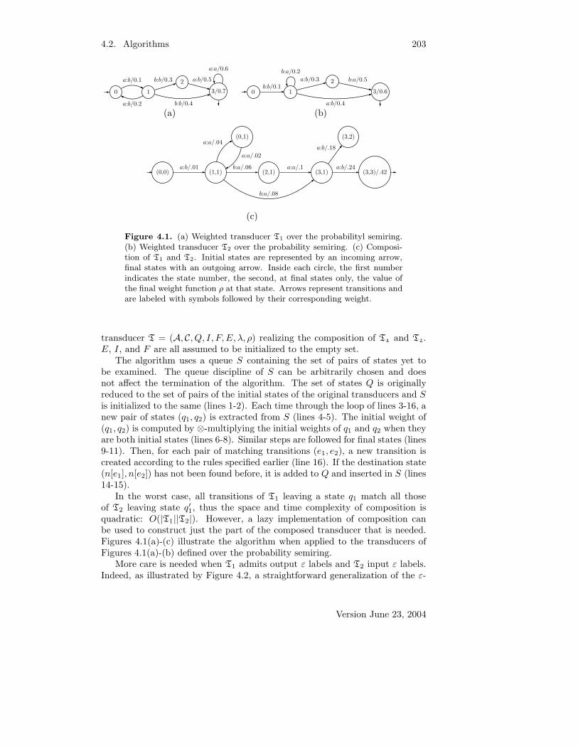
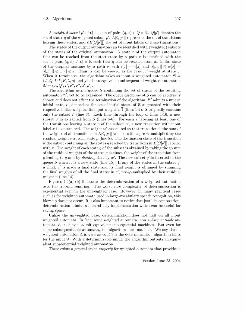
Figures 4.4(a)-(b) illustrate the determinization of a weighted automatonover the tropical semiring. The worst case complexity of determinization isexponential even in the unweighted case. However, in many practical casessuch as for weighted automata used in large-vocabulary speech recognition, thisblow-up does not occur. It is also important to notice that just like composition,determinization admits a natural lazy implementation which can be useful forsaving space.

Unlike the unweighted case, determinization does not halt on all inputweighted automata. In fact, some weighted automata, non subsequentiable au-tomata, do not even admit equivalent subsequential machines. But even forsome subsequentiable automata, the algorithm does not halt. We say that aweighted automaton A is determinizable if the determinization algorithm haltsfor the input A. With a determinizable input, the algorithm outputs an equiv-alent subsequential weighted automaton.

There exists a general twins property for weighted automata that provides a



0

1

2

3

a/1

a/2

c/5

d/6

b/3

b/3 (0,0) (1,0),(2,1) (3,0)/0a/1

c/5

d/7

b/3

0

1

2

3

a/1

a/2

c/5

d/6

b/3

b/4

(a) (b) (c)

Figure 4.4. Determinization of weighted automata. (a) Weighted au-tomaton over the tropical semiring A. (b) Equivalent weighted automatonB obtained by determinization of A. (c) Non-determinizable weighted au-tomaton over the tropical semiring, states 1 and 2 are non-twin siblings.

characterization of determinizable weighted automata under some general con-ditions. Let A be a weighted automaton over a weakly left divisible left semiringK. Two states q and q′ of A are said to be siblings if there exist two strings xand y in A∗ such that both q and q′ can be reached from I by paths labeledwith x and there is a cycle at q and a cycle at q′ both labeled with y. WhenK is a commutative and cancellative semiring, two sibling states are said to betwins iff for any string y:

w[P (q, y, q)] = w[P (q′, y, q′)] (4.2.5)

A has the twins property if any two sibling states of A are twins. Figure 4.4(c)shows an unambiguous weighted automaton over the tropical semiring that doesnot have the twins property: states 1 and 2 can be reached by paths labeledwith a from the initial state and admit cycles with the same label b, but theweights of these cycles (3 and 4) are different.

Theorem 4.2.2. Let A be a weighted automaton over the tropical semiring.If A has the twins property, then A is determinizable.

With trim unambiguous weighted automata, the condition is also necessary.

Theorem 4.2.3. Let A be a trim unambiguous weighted automaton over thetropical semiring. Then the three following properties are equivalent:

1. A is determinizable.2. A has the twins property.3. A is subsequentiable.

There exists an efficient algorithm for testing the twins property for weightedautomata, which cannot be presented briefly in this chapter. Note that anyacyclic weighted automaton over a zero-sum-free semiring has the twins propertyand is determinizable.


4.2. Algorithms 209

4.2.3. Weight pushing

The choice of the distribution of the total weight along each successful path ofa weighted automaton does not affect the definition of the function realized bythat automaton, but this may have a critical impact on the efficiency in manyapplications, e.g., natural language processing applications, when a heuristicpruning is used to visit only a subpart of the automaton. There exists analgorithm, weight pushing, for normalizing the distribution of the weights alongthe paths of a weighted automaton or more generally a weighted directed graph.The transducer normalization algorithm presented in Chapter 1 Section 1.5 canbe viewed as a special instance of this algorithm.

Let A be a weighted automaton over a semiring K. Assume that K is zero-sum-free and weakly left divisible. For any state q ∈ Q, assume that the follow-ing sum is well-defined and in K:

d[q] =⊕

π∈P (q,F )

(w[π] ⊗ ρ[n[π]]) (4.2.6)

d[q] is the shortest-distance from q to F . d[q] is well-defined for all q ∈ Q when K

is a k-closed semiring. The weight pushing algorithm consists of computing eachshortest-distance d[q] and of reweighting the transition weights, initial weightsand final weights in the following way:

∀e ∈ E s.t. d[p[e]] 6= 0, w[e] ← d[p[e]]−1 ⊗ w[e]⊗ d[n[e]] (4.2.7)

∀q ∈ I, λ[q] ← λ[q]⊗ d[q] (4.2.8)

∀q ∈ F, s.t. d[q] 6= 0, ρ[q] ← d[q]−1 ⊗ ρ[q] (4.2.9)

Each of these operations can be assumed to be done in constant time, thusreweighting can be done in linear time O(T⊗|A|) where T⊗ denotes the worstcost of an ⊗-operation. The complexity of the computation of the shortest-distances depends on the semiring. In the case of k-closed semirings such as thetropical semiring, d[q], q ∈ Q, can be computed using a generic shortest-distancealgorithm. The complexity of the algorithm is linear in the case of an acyclicautomaton: O(Card(Q)+(T⊕+T⊗)Card(E)), where T⊕ denotes the worst costof an ⊕-operation. In the case of a general weighted automaton over the tropicalsemiring, the complexity of the algorithm is O(Card(E)+Card(Q) log Card(Q)).

In the case of closed semirings such as (R+, +,×, 0, 1), a generalization ofthe Floyd-Warshall algorithm for computing all-pairs shortest-distances can beused. The complexity of the algorithm is Θ(Card(Q)3(T⊕+T⊗+T∗)) where T∗

denotes the worst cost of the closure operation. The space complexity of thesealgorithms is Θ(Card(Q)2). These complexities make it impractical to use theFloyd-Warshall algorithm for computing d[q], q ∈ Q, for relatively large graphsor automata of several hundred million states or transitions. An approximateversion of a generic shortest-distance algorithm can be used instead to computed[q] efficiently.

Roughly speaking, the algorithm pushes the weights of each path as much aspossible towards the initial states. Figures 4.5(a)-(c) illustrate the applicationof the algorithm in a special case both for the tropical and probability semirings.



0

1

2

3

a/0

b/1

c/5

d/0

e/1

e/0

f/1

e/4

f/5

0/0

1

2

3/0

a/0

b/1

c/5

d/4

e/5

e/0

f/1

e/0

f/1

0/15

1

2

3/1

a/0

b/ 115

c/ 515

d/0

e/ 915

e/0

f/1

e/49

f/59

0/0 1 3/0

a/0

b/1

c/5

e/0

f/1

(a) (b) (c) (d)

Figure 4.5. Weight pushing algorithm. (a) Weighted automaton A.(b) Equivalent weighted automaton B obtained by weight pushing in thetropical semiring. (c) Weighted automaton C obtained from A by weightpushing in the probability semiring. (d) Minimal weighted automatonover the tropical semiring equivalent to A.

Note that if d[q] = 0, then, since K is zero-sum-free, the weight of all pathsfrom q to F is 0. Let A be a weighted automaton over the semiring K. Assumethat K is closed or k-closed and that the shortest-distances d[q] are all well-defined and in K−

{

0}

. Note that in both cases we can use the distributivity overthe infinite sums defining shortest distances. Let e′ (π′) denote the transition e(path π) after application of the weight pushing algorithm. e′ (π′) differs frome (resp. π) only by its weight. Let λ′ denote the new initial weight function,and ρ′ the new final weight function.

Proposition 4.2.4. Let B = (A, Q, I, F, E′, λ′, ρ′) be the result of the weightpushing algorithm applied to the weighted automaton A, then

1. the weight of a successful path π is unchanged after application of weightpushing:

λ′[p[π′]]⊗ w[π′]⊗ ρ′[n[π′]] = λ[p[π]]⊗ w[π] ⊗ ρ[n[π]] (4.2.10)

2. the weighted automaton B is stochastic, i.e.

∀q ∈ Q,⊕

e′∈E′[q]

w[e′] = 1 (4.2.11)

Proof. Let π′ = e′1 . . . e′k. By definition of λ′ and ρ′,

λ′[p[π′]] ⊗ w[π′] ⊗ ρ

′[n[π′]] = λ[p[e1]] ⊗ d[p[e1]] ⊗ d[p[e1]]−1

⊗ w[e1] ⊗ d[n[e1]] ⊗ · · ·

⊗ d[p[ek]]−1⊗ w[ek] ⊗ d[n[ek]] ⊗ d[n[ek]]−1

⊗ ρ[n[π]]

= λ[p[π]] ⊗ w[e1] ⊗ · · · ⊗ w[ek] ⊗ ρ[n[π]]

which proves the first statement of the proposition. Let q ∈ Q,M

e′∈E′[q]

w[e′] =M

e∈E[q]

d[q]−1⊗ w[e] ⊗ d[n[e]]

= d[q]−1⊗

M

e∈E[q]

w[e] ⊗ d[n[e]]


4.2. Algorithms 211

= d[q]−1⊗

M

e∈E[q]

w[e] ⊗M

π∈P (n[e],F )

(w[π] ⊗ ρ[n[π]])

= d[q]−1⊗

M

e∈E[q],π∈P (n[e],F )

(w[e] ⊗ w[π] ⊗ ρ[n[π]])

= d[q]−1⊗ d[q] = 1

where we used the distributivity of the multiplicative operation over infinitesums in closed or k-closed semirings. This proves the second statement of theproposition.

These two properties of weight pushing are illustrated by Figures 4.5(a)-(c): thetotal weight of a successful path is unchanged after pushing; at each state ofthe weighted automaton of Figure 4.5(b), the minimum weight of the outgoingtransitions is 0, and at at each state of the weighted automaton of Figure 4.5(c),the weights of outgoing transitions sum to 1. Weight pushing can also be usedto test the equivalence of two weighted automata.

4.2.4. Minimization

A deterministic weighted automaton is said to be minimal if there exists no otherdeterministic weighted automaton with a smaller number of states and realizingthe same function. Two states of a deterministic weighted automaton are said tobe equivalent if exactly the same set of strings with the same weights label pathsfrom these states to a final state, the final weights being included. Thus, twoequivalent states of a deterministic weighted automaton can be merged withoutaffecting the function realized by that automaton. A weighted automaton isminimal when it admits no two distinct equivalent states after any redistributionof the weights along its paths.

There exists a general algorithm for computing a minimal deterministic au-tomaton equivalent to a given weighted automaton. It is thus a generalizationof the minimization algorithms for unweighted finite automata. It can be com-bined with the minimization algorithm for unweighted finite-state transducerspresented in Chapter 1 Section 1.5 to minimize weighted finite-state transduc-ers.3 It consists of first applying the weight pushing algorithm to normalize thedistribution of the weights along the paths of the input automaton, and thenof treating each pair (label, weight) as a single label and applying the classical(unweighted) automata minimization.

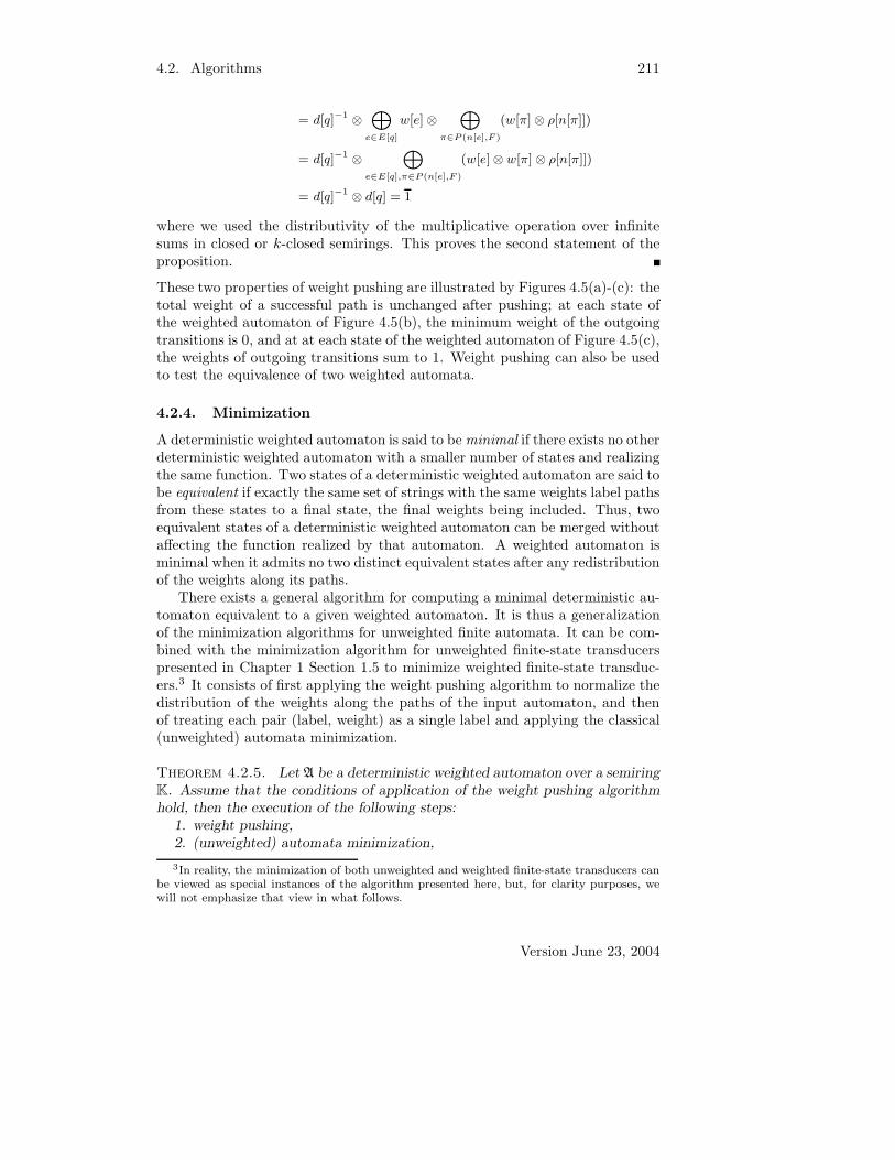
Theorem 4.2.5. Let A be a deterministic weighted automaton over a semiringK. Assume that the conditions of application of the weight pushing algorithmhold, then the execution of the following steps:

1. weight pushing,2. (unweighted) automata minimization,

3In reality, the minimization of both unweighted and weighted finite-state transducers canbe viewed as special instances of the algorithm presented here, but, for clarity purposes, wewill not emphasize that view in what follows.



0

1

2

3/1

a/1

b/2

c/3

d/4

e/5

e/.8

f/1

e/4

f/5

0/4595 1 2/1

a/ 151

b/ 251

c/ 351

d/ 2051

e/ 2551

e/ 49

f/ 59

0/25 1 2/1

a/.04

b/.08

c/.12

d/.80

e/1.0

e/0.8

f/1.0

(a) (b) (c)

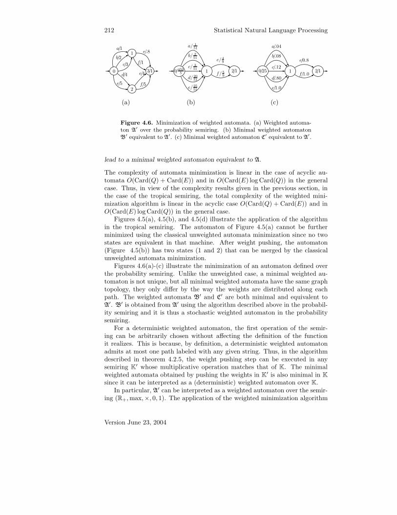
Figure 4.6. Minimization of weighted automata. (a) Weighted automa-ton A′ over the probability semiring. (b) Minimal weighted automatonB′ equivalent to A′. (c) Minimal weighted automaton C′ equivalent to A′.

lead to a minimal weighted automaton equivalent to A.

The complexity of automata minimization is linear in the case of acyclic au-tomata O(Card(Q) + Card(E)) and in O(Card(E) log Card(Q)) in the generalcase. Thus, in view of the complexity results given in the previous section, inthe case of the tropical semiring, the total complexity of the weighted mini-mization algorithm is linear in the acyclic case O(Card(Q) + Card(E)) and inO(Card(E) log Card(Q)) in the general case.

Figures 4.5(a), 4.5(b), and 4.5(d) illustrate the application of the algorithmin the tropical semiring. The automaton of Figure 4.5(a) cannot be furtherminimized using the classical unweighted automata minimization since no twostates are equivalent in that machine. After weight pushing, the automaton(Figure 4.5(b)) has two states (1 and 2) that can be merged by the classicalunweighted automata minimization.

Figures 4.6(a)-(c) illustrate the minimization of an automaton defined overthe probability semiring. Unlike the unweighted case, a minimal weighted au-tomaton is not unique, but all minimal weighted automata have the same graphtopology, they only differ by the way the weights are distributed along eachpath. The weighted automata B′ and C′ are both minimal and equivalent toA′. B′ is obtained from A′ using the algorithm described above in the probabil-ity semiring and it is thus a stochastic weighted automaton in the probabilitysemiring.

For a deterministic weighted automaton, the first operation of the semir-ing can be arbitrarily chosen without affecting the definition of the functionit realizes. This is because, by definition, a deterministic weighted automatonadmits at most one path labeled with any given string. Thus, in the algorithmdescribed in theorem 4.2.5, the weight pushing step can be executed in anysemiring K

′ whose multiplicative operation matches that of K. The minimalweighted automata obtained by pushing the weights in K

′ is also minimal in K

since it can be interpreted as a (deterministic) weighted automaton over K.In particular, A′ can be interpreted as a weighted automaton over the semir-

ing (R+, max,×, 0, 1). The application of the weighted minimization algorithm


4.3. Application to speech recognition 213

to A′ in this semiring leads to the minimal weighted automaton C′ of Fig-ure 4.6(c). C′ is also a stochastic weighted automaton in the sense that, at anystate, the maximum weight of all outgoing transitions is one.

This fact leads to several interesting observations. One is related to thecomplexity of the algorithms. Indeed, we can choose a semiring K

′ in whichthe complexity of weight pushing is better than in K. The resulting automatonis still minimal in K and has the additional property of being stochastic in K

′.It only differs from the weighted automaton obtained by pushing weights inK in the way weights are distributed along the paths. They can be obtainedfrom each other by application of weight pushing in the appropriate semiring.In the particular case of a weighted automaton over the probability semiring,it may be preferable to use weight pushing in the (max,×)-semiring since thecomplexity of the algorithm is then equivalent to that of classical single-sourceshortest-paths algorithms. The corresponding algorithm is a special instance ofthe generic shortest-distance algorithm.

Another important point is that the weight pushing algorithm may not bedefined in K because the machine is not zero-sum-free or for other reasons.But an alternative semiring K

′ can sometimes be used to minimize the inputweighted automaton.

The results just presented were all related to the minimization of the num-ber of states of a deterministic weighted automaton. The following propositionshows that minimizing the number of states coincides with minimizing the num-ber of transitions.

Proposition 4.2.6. Let A be a minimal deterministic weighted automaton,then A has the minimal number of transitions.

Proof. Let A be a deterministic weighted automaton with the minimal numberof transitions. If two distinct states of A were equivalent, they could be merged,thereby strictly reducing the number of its transitions. Thus, A must be aminimal deterministic automaton. Since, minimal deterministic automata havethe same topology, in particular the same number of states and transitions, thisproves the proposition.

4.3. Application to speech recognition

Much of the statistical techniques now widely used in natural language process-ing were inspired by early work in speech recognition. This section discussesthe representation of the component models of an automatic speech recogni-tion system by weighted transducers and describes how they can be combined,searched, and optimized using the algorithms described in the previous sec-tions. The methods described can be used similarly in many other areas ofnatural language processing.



4.3.1. Statistical formulation

Speech recognition consists of generating accurate written transcriptions for spo-ken utterances. The desired transcription is typically a sequence of words, but itmay also be the utterance’s phonemic or syllabic transcription or a transcriptioninto any other sequence of written units.

The problem can be formulated as a maximum-likelihood decoding problem,or the so-called noisy channel problem. Given a speech utterance, speech recog-nition consists of determining its most likely written transcription. Thus, if welet o denote the observation sequence produced by a signal processing system, wa (word) transcription sequence over an alphabet A, and P(w | o) the probabil-ity of the transduction of o into w, the problem consists of finding w as definedby:

w = argmaxw∈A∗

P(w | o) (4.3.1)

Using Bayes’ rule, P(w | o) can be rewritten as: P(o|w)P(w)P(o) . Since P(o) does

not depend on w, the problem can be reformulated as:

w = argmaxw∈A∗

P(o | w)P(w) (4.3.2)

where P(w) is the a priori probability of the written sequence w in the languageconsidered and P(o | w) the probability of observing o given that the sequencew has been uttered. The probabilistic model used to estimate P(w) is calleda language model or a statistical grammar. The generative model associatedto P(o | w) is a combination of several knowledge sources, in particular theacoustic model, and the pronunciation model. P(o | w) can be decomposed intoseveral intermediate levels e.g., that of phones, syllables, or other units. In mostlarge-vocabulary speech recognition systems, it is decomposed into the followingprobabilistic models that are assumed independent:

• P(p | w), a pronunciation model or lexicon transducing word sequences wto phonemic sequences p;

• P(c | p), a context-dependency transduction mapping phonemic sequencesp to context-dependent phone sequences c;

• P(d | c), a context-dependent phone model mapping sequences of context-dependent phones c to sequences of distributions d; and

• P(o | d), an acoustic model applying distribution sequences d to observa-tion sequences.4

Since the models are assumed to be independent,

P(o | w) =∑

d,c,p

P(o | d)P(d | c)P(c | p)P(p | w) (4.3.3)

4P(o | d)P(d | c) or P(o | d)P(d | c)P(c | p) is often called an acoustic model.



Equation 4.3.2 can thus be rewritten as:

w = argmaxw

∑

d,c,p

P(o | d)P(d | c)P(c | p)P(p | w)P(w) (4.3.4)

The following sections discuss the definition and representation of each of thesemodels and that of the observation sequences in more detail. The transductionmodels are typically given either directly or as a result of an approximation asweighted finite-state transducers. Similarly, the language model is representedby a weighted automaton.

4.3.2. Statistical grammar

In some relatively restricted tasks, the language model for P(w) is based onan unweighted rule-based grammar. But, in most large-vocabulary tasks, themodel is a weighted grammar derived from large corpora of several million wordsusing statistical methods. The purpose of the model is to assign a probabilityto each sequence of words, thereby assigning a ranking to all sequences. Thus,the parsing information it may supply is not directly relevant to the statisticalformulation described in the previous section.

The probabilistic model derived from corpora may be a probabilistic context-free grammmar. But, in general, context-free grammars are computationallytoo demanding for real-time speech recognition systems. The amount of workrequired to expand a recognition hypothesis can be unbounded for an unre-stricted grammar. Instead, a regular approximation of a probabilistic context-free grammar is used. In most large-vocabulary speech recognition systems, theprobabilistic model is in fact directly constructed as a weighted regular gram-mar and represents an n-gram model. Thus, this section concentrates on a briefdescription of these models.5

Regardless of the structure of the model, using the Bayes’s rule, the probabil-ity of the word sequence w = w1 · · ·wk can be written as the following productof conditional probabilities:

P(w) =

k∏

i=1

P(wi | w1 · · ·wi−1) (4.3.5)

An n-gram model is based on the Markovian assumption that the probabilityof the occurrence of a word only depends on the n− 1 preceding words, that is,for i = 1 . . . n:

P(wi | w1 · · ·wi−1) = P(wi | hi) (4.3.6)

where the conditioning history hi has length at most n− 1: |hi| ≤ n− 1. Thus,

P(w) =

k∏

i=1

P(wi | hi) (4.3.7)

5Similar probabilistic models are designed for biological sequences (see Chapter 6).



wi−2wi−1 wi−1wi

wi−1 wi

ε

wi

wi

wi−1Φ Φ

Φ

0

1/8.318

2/1.386

3

bye/8.318

hello/7.625

ε/-0.287

ε/-1.386 bye/0.693

hello/1.386

bye/7.625

ε/-0.693

(a) (b)

Figure 4.7. Katz back-off n-gram model. (a) Representation of a trigrammodel with failure transitions labeled with Φ. (b) Bigram model derivedfrom the input text hello bye bye. The automaton is defined over the logsemiring (the transition weights are negative log-probabilities). State 0 isthe initial state. State 1 corresponds to the word bye and state 3 to theword hello. State 2 is the back-off state.

Let c(w) denote the number of occurrences of a sequence w in the corpus. c(hi)and c(hiwi) can be used to estimate the conditional probability P(wi | hi).When c(hi) 6= 0, the maximum likelihood estimate of P(wi | hi) is:

P(wi | hi) =c(hiwi)

c(hi)(4.3.8)

But, a classical data sparsity problem arises in the design of all n-gram models:the corpus, no matter how large, may contain no occurrence of hi (c(hi) = 0).A solution to this problem is based on smoothing techniques. This consists ofadjusting P to reserve some probability mass for unseen n-gram sequences.

Let P(wi | hi) denote the adjusted conditional probability. A smoothingtechnique widely used in language modeling is the Katz back-off technique.The idea is to “back-off” to lower order n-gram sequences when c(hiwi) = 0.Define the backoff sequence of hi as the lower order n-gram sequence suffix ofhi and denote it by h′

i. hi = uh′i for some word u. Then, in a Katz back-off

model, P(wi | hi) is defined as follows:

P(wi | hi) =

{

P(wi | hi) if c(hiwi) > 0αhi

P(wi | h′i) otherwise

(4.3.9)

where αhiis a factor ensuring normalization. The Katz back-off model admits a

natural representation by a weighted automaton in which each state encodes a



0 1 2 3 4/1d:ε/1.0

ey:ε/0.8

ae:ε/0.2

dx:ε/0.6

t:ε/0.4

ax:data/1.0

Figure 4.8. Section of a pronunciation model of English, a weightedtransducer over the probability semiring giving a compact representationof four pronunciations of the word data due to two distinct pronunciationsof the first vowel a and two pronunciations of the consonant t (flapped ornot).

conditioning history of length less than n. As in the classical de Bruijn graphs,there is a transition labeled with wi from the state encoding hi to the stateencoding h′

iwi when c(hiwi) 6= 0. A so-called failure transition can be used tocapture the semantic of “otherwise” in the definition of the Katz back-off modeland keep its representation compact. A failure transition is a transition taken atstate q when no other transition leaving q has the desired label. Figure 4.3.2(a)illustrates that construction in the case of a trigram model (n = 3).

It is possible to give an explicit representation of these weighted automatawithout using failure transitions. However, the size of the resulting automatamay become prohibitive. Instead, an approximation of that weighted automatonis used where failure transitions are simply replaced by ε-transitions. This turnsout to cause only a very limited loss in accuracy.6.

In practice, for numerical instability reasons negative-log probabilities areused and the language model weighted automaton is defined in the log semiring.Figure 4.3.2(b) shows the corresponding weighted automaton in a very simplecase. We will denote by G the weighted automaton representing the statisticalgrammar.

4.3.3. Pronunciation model

The representation of a pronunciation model P(p | w) (or lexicon) with weightedtransducers is quite natural. Each word has a finite number of phonemic tran-scriptions. The probability of each pronunciation can be estimated from a cor-pus. Thus, for each word x, a simple weighted transducer Tx mapping x to itsphonemic transcriptions can be constructed.

Figure 4.8 shows that representation in the case of the English word data.The closure of the union of the transducers Tx for all the words x consideredgives a weighted transducer representation of the pronunciation model. We willdenote by P the equivalent transducer over the log semiring.

6An alternative when no offline optimization is used is to compute the explicit represen-tation on-the-fly, as needed for the recognition of an utterance. There exists also a complexmethod for constructing an exact representation of an n-gram model which cannot be pre-sented in this short chapter.



(ε,C)

(p,p)

(q,q)

(p,q)

(q,p)

(p,ε)

(q,ε)

εpp:p/0

εqp:q/0

εqq:q/0

εpq:p/0εpε:p/0

εqε:q/0

ppp:p/0

qqq:q/0

ppq:p/0

qqp:q/0

ppε:p/0

qqε:q/0

pqq:q/0

pqp:q/0

pqε:q/0

qpp:p/0

qpq:p/0

qpε:p/0

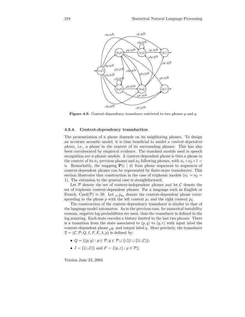
Figure 4.9. Context-dependency transducer restricted to two phones p and q.

4.3.4. Context-dependency transduction

The pronunciation of a phone depends on its neighboring phones. To designan accurate acoustic model, it is thus beneficial to model a context-dependent

phone, i.e., a phone in the context of its surrounding phones. This has alsobeen corroborated by empirical evidence. The standard models used in speechrecognition are n-phonic models. A context-dependent phone is then a phone inthe context of its n1 previous phones and n2 following phones, with n1+n2+1 =n. Remarkably, the mapping P(c | d) from phone sequences to sequences ofcontext-dependent phones can be represented by finite-state transducers. Thissection illustrates that construction in the case of triphonic models (n1 = n2 =1). The extension to the general case is straightforward.

Let P denote the set of context-independent phones and let C denote theset of triphonic context-dependent phones. For a language such as English orFrench, Card(P) ≈ 50. Let p1

pp2denote the context-dependent phone corre-

sponding to the phone p with the left context p1 and the right context p2.The construction of the context-dependency transducer is similar to that of

the language model automaton. As in the previous case, for numerical instabilityreasons, negative log-probabilities are used, thus the transducer is defined in thelog semiring. Each state encodes a history limited to the last two phones. Thereis a transition from the state associated to (p, q) to (q, r) with input label thecontext-dependent phone pqr and output label q. More precisely, the transducerT = (C,P , Q, I, F, E, λ, ρ) is defined by:

• Q = {(p, q) : p ∈ P , q ∈ P ∪ {ε}} ∪ {(ε, C)};

• I = {(ε, C)} and F = {(p, ε) : p ∈ P};



0 1 2 3

d1:ε d2:ε d3:ε

d1:ε d2:ε d3:pqr

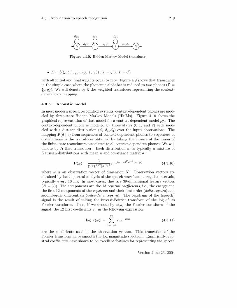
Figure 4.10. Hidden-Markov Model transducer.

• E ⊆ {((p, Y ), pqr, q, 0, (q, r)) : Y = q or Y = C}

with all initial and final weights equal to zero. Figure 4.9 shows that transducerin the simple case where the phonemic alphabet is reduced to two phones (P ={p, q}). We will denote by C the weighted transducer representing the context-dependency mapping.

4.3.5. Acoustic model

In most modern speech recognition systems, context-dependent phones are mod-eled by three-state Hidden Markov Models (HMMs). Figure 4.10 shows thegraphical representation of that model for a context-dependent model pqr. Thecontext-dependent phone is modeled by three states (0, 1, and 2) each mod-eled with a distinct distribution (d0, d1, d2) over the input observations. Themapping P(d | c) from sequences of context-dependent phones to sequences ofdistributions is the transducer obtained by taking the closure of the union ofthe finite-state transducers associated to all context-dependent phones. We willdenote by H that transducer. Each distribution di is typically a mixture ofGaussian distributions with mean µ and covariance matrix σ:

P(ω) =1

(2π)N/2|σ|1/2e−

1

2(ω−µ)T σ−1(ω−µ) (4.3.10)

where ω is an observation vector of dimension N . Observation vectors areobtained by local spectral analysis of the speech waveform at regular intervals,typically every 10 ms. In most cases, they are 39-dimensional feature vectors(N = 39). The components are the 13 cepstral coefficients, i.e., the energy andthe first 12 components of the cepstrum and their first-order (delta cepstra) andsecond-order differentials (delta-delta cepstra). The cepstrum of the (speech)signal is the result of taking the inverse-Fourier transform of the log of itsFourier transform. Thus, if we denote by x(ω) the Fourier transform of thesignal, the 12 first coefficients cn in the following expression:

log |x(ω)| =∞∑

n=−∞

cne−inω (4.3.11)

are the coefficients used in the observation vectors. This truncation of theFourier transform helps smooth the log magnitude spectrum. Empirically, cep-stral coefficients have shown to be excellent features for representing the speech



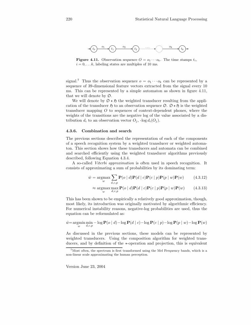
t0 t1 t2 tko1 o2 . . . ok

Figure 4.11. Observation sequence O = o1 · · · ok. The time stamps ti,i = 0, . . . k, labeling states are multiples of 10 ms.

signal.7 Thus the observation sequence o = o1 · · · ok can be represented by asequence of 39-dimensional feature vectors extracted from the signal every 10ms. This can be represented by a simple automaton as shown in figure 4.11,that we will denote by O.

We will denote by O ? H the weighted transducer resulting from the appli-cation of the transducer H to an observation sequence O. O ? H is the weightedtransducer mapping O to sequences of context-dependent phones, where theweights of the transitions are the negative log of the value associated by a dis-tribution di to an observation vector Oj , -log di(Oj).

4.3.6. Combination and search

The previous sections described the representation of each of the componentsof a speech recognition system by a weighted transducer or weighted automa-ton. This section shows how these transducers and automata can be combinedand searched efficiently using the weighted transducer algorithms previouslydescribed, following Equation 4.3.4.

A so-called Viterbi approximation is often used in speech recognition. Itconsists of approximating a sum of probabilities by its dominating term:

w = argmaxw

∑

d,c,p

P(o | d)P(d | c)P(c | p)P(p | w)P(w) (4.3.12)

≈ argmaxw

maxd,c,p

P(o | d)P(d | c)P(c | p)P(p | w)P(w) (4.3.13)

This has been shown to be empirically a relatively good approximation, though,most likely, its introduction was originally motivated by algorithmic efficiency.For numerical instability reasons, negative-log probabilities are used, thus theequation can be reformulated as:

w=argminw

mind,c,p− logP(o | d)−logP(d | c)−logP(c | p)−logP(p | w)−logP(w)

As discussed in the previous sections, these models can be represented byweighted transducers. Using the composition algorithm for weighted trans-ducers, and by definition of the ?-operation and projection, this is equivalent

7Most often, the spectrum is first transformed using the Mel Frequency bands, which is anon-linear scale approximating the human perception.



HMM Transducer H CD Transducer C Pron. Model P Grammar Gobservations O CD phones CI phones words words

Figure 4.12. Cascade of speech recognition transducers.

to:8

w = argminw

Π2(O ? H ◦ C ◦P ◦G) (4.3.14)

Thus, speech recognition can be formulated as a cascade of composition ofweighted transducers illustrated by Figure 4.12. w labels the path of W =Π2(O ? H ◦ C ◦ P ◦ G) with the lowest weight. The problem can be viewed asa classical single-source shortest-paths algorithm over the weighted automatonW. Any single-source shortest paths algorithm could be used to solve it. Infact, since O is finite, the automaton W could be acyclic, in which case the clas-sical linear-time single-source shortest-paths algorithm based on the topologicalorder could be used.

However, this scheme is not practical. This is because the size of W canbe prohibitively large even for recognizing short utterances. The number oftransitions of O for 10s of speech is 1000. If the recognition transducer T =H ◦ C ◦P ◦G had in the order of just 100M transitions, the size of W would bein the order of 1000× 100M transitions, i.e., about 100 billion transitions!

In practice, instead of visiting all states and transitions, a heuristic pruningis used. A pruning technique often used is the beam search. This consists ofexploring only states with tentative shortest-distance weights within a beam orthreshold of the weight of the best comparable state. Comparable states mustroughly correspond to the same observations, thus states of T are visited in theorder of analysis of the input observation vectors, i.e. chronologically. Thisis referred to as a synchronous beam search. A synchronous search restrictsthe choice of the single-source shortest-paths problem or the relaxation of thetentative shortest-distances. The specific single-source shortest paths algorithmthen used is known as the Viterbi Algorithm, which is presented in Exercise1.3.1.

The ?-operation, the Viterbi algorithm, and the beam pruning techniquesare often combined into a decoder. Here is a brief description of the decoder.For each observation vector oi read, the transitions leaving the current states ofT are expanded, the ?-operation is computed on-the-fly to compute the acousticweights given by the application of the distributions to oi. The acoustic weightsare added to the existing weight of the transitions and out of the set of states

8Note that the Viterbi approximation can be viewed simply as a change of semiring, fromthe log semiring to the tropical semiring. This does not affect the topology or the weightsof the transducers but only their interpretation or use. Also, note that composition does notmake use of the first operation of the semiring, thus compositions in the log and tropicalsemiring coincide.



reached by these transitions those with a tentative shortest-distance beyond apre-determined threshold are pruned out. The beam threshold can be used as ameans to select a trade-off between recognition speed and accuracy. Note thatthe pruning technique used is non-admissible. The best overall path may fallout of the beam due to local comparisons.

4.3.7. Optimizations

The characteristics of the recognition transducer T were left out of the previousdiscussion. They are however key parameters for the design of real-time large-vocabulary speech recognition systems. The search and decoding speed criticallydepends on the size of T and its non-determinism. This section describes theuse of the determinization, minimization, and weight pushing algorithm forconstructing and optimizing T.

The component transducers described can be very large in speech recognitionapplications. The weighted automata and transducers we used in the NorthAmerican Business news (NAB) dictation task with a vocabulary of just 40,000words (the full vocabulary in this task contains about 500,000 words) had thefollowing attributes:

• G: a shrunk Katz back-off trigram model with about 4M transitions;9

• P : pronunciation transducer with about 70, 000 states and more than150,000 transitions;

• C: a triphonic context-dependency transducer with about 1,500 states and80,000 transitions.

• H: an HMM transducer with more than 7,000 states.

A full construction of T by composition of such transducers without anyoptimization is not possible even when using very large amounts of memory.Another problem is the non-determinism of T. Without prior optimization, T ishighly non-deterministic, thus, a large number of paths need to be explored atthe search and decoding time, thereby considerably slowing down recognition.

Weighted determinization and minimization algorithms provide a generalsolution to both the non-determinism and the size problem. To construct anoptimized recognition transducer, weighted transducer determinization and min-imization can be used at each step of the composition of each pair of componenttransducers. The main purpose of the use of determinization is to eliminatenon-determinism in the resulting transducer, thereby substantially reducingrecognition time. But, its use at intermediate steps of the construction alsohelps improve the efficiency of composition and reduce the size of the resultingtransducer. We will see later that it is in fact possible to construct offline therecognition transducer and that its size is practical for real-time speech recog-nition!

9Various shrinking methods can be used to reduce the size of a statistical grammar withoutaffecting its accuracy excessively.



However, as pointed out earlier, not all weighted automata and transducersare determinizable, e.g., the transducer P◦G mapping phone sequences to wordsis in general not determinizable. This is clear in presence of homophones. Buteven in the absence of homophones, P◦G may not have the twins property andbe non-determinizable. To make it possible to determinize P ◦G, an auxiliaryphone symbol denoted by #0 marking the end of the phonemic transcription ofeach word can be introduced. Additional auxiliary symbols #1 . . .#k−1 can beused when necessary to distinguish homophones as in the following example:

r eh d #0 read

r eh d #1 red

At most D auxiliary phones, where D is the maximum degree of homophony,are introduced. The pronunciation transducer augmented with these auxiliarysymbols is denoted by P. For consistency, the context-dependency transducerC must also accept all paths containing these new symbols. For further deter-minizations at the context-dependent phone level and distribution level, eachauxiliary phone must be mapped to a distinct context-dependent phone. Thus,self-loops are added at each state of C mapping each auxiliary phone to a newauxiliary context-dependent phone. The augmented context-dependency trans-ducer is denoted by C.

Similarly, each auxiliary context-dependent phone must be mapped to a newdistinct distribution. D self-loops are added at the initial state of H with aux-iliary distribution input labels and auxiliary context-dependency output labelsto allow for this mapping. The modified HMM transducer is denoted by H.

It can be shown that the use of the auxiliary symbols guarantees the de-terminizability of the transducer obtained after each composition. Weightedtransducer determinization is used at several steps of the construction. An n-gram language model G is often constructed directly as a deterministic weightedautomaton with a back-off state – in this context, the symbol ε is treated asa regular symbol for the definition of determinism. If this does not hold, G isfirst determinized. P is then composed with G and determinized: det(P ◦G).The benefit of this determinization is the reduction of the number of alternativetransitions at each state to at most the number of distinct phones at that state(≈ 50), while the original transducer may have as many as V outgoing transi-tions at some states where V is the vocabulary size. For large tasks where thevocabulary size can be more than several hundred thousand, the advantage ofthis optimization is clear.

The inverse of the context-dependency transducer might not be determin-istic.10 For example, the inverse of the transducer shown in Figure 4.9 is notdeterministic since the initial state admits several outgoing transitions with thesame input label p or q. To construct a small and efficient integrated transducer,it is important to first determinize the inverse of C.11

10The inverse of a transducer is the transducer obtained by swapping input and outputlabels of all transitions.

11Triphonic or more generally n-phonic context-dependency models can also be constructeddirectly with a deterministic inverse.



C is then composed with the resulting transducer and determinized. Simi-larly H is composed with the context-dependent transducer and determinized.This last determinization increases sharing among HMM models that start withthe same distributions: at each state of the resulting integrated transducer,there is at most one outgoing transition labeled with any given distributionname. This leads to a substantial reduction of the recognition time.

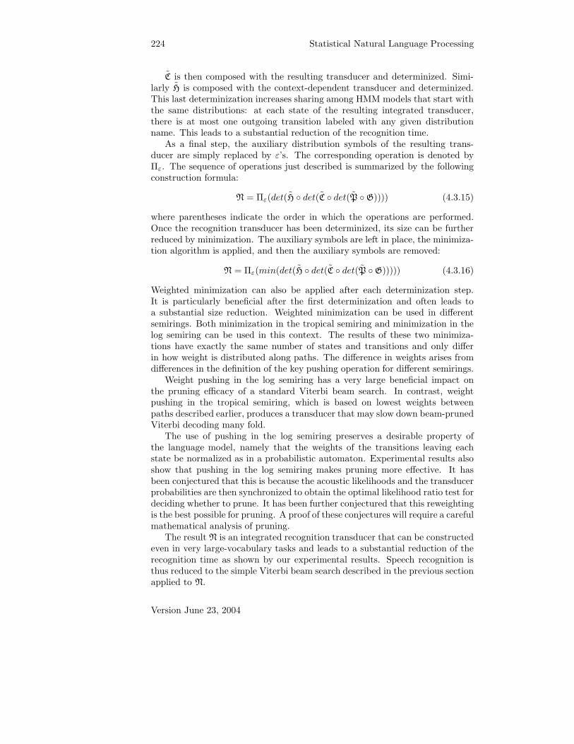
As a final step, the auxiliary distribution symbols of the resulting trans-ducer are simply replaced by ε’s. The corresponding operation is denoted byΠε. The sequence of operations just described is summarized by the followingconstruction formula:

N = Πε(det(H ◦ det(C ◦ det(P ◦G)))) (4.3.15)

where parentheses indicate the order in which the operations are performed.Once the recognition transducer has been determinized, its size can be furtherreduced by minimization. The auxiliary symbols are left in place, the minimiza-tion algorithm is applied, and then the auxiliary symbols are removed:

N = Πε(min(det(H ◦ det(C ◦ det(P ◦G))))) (4.3.16)

Weighted minimization can also be applied after each determinization step.It is particularly beneficial after the first determinization and often leads toa substantial size reduction. Weighted minimization can be used in differentsemirings. Both minimization in the tropical semiring and minimization in thelog semiring can be used in this context. The results of these two minimiza-tions have exactly the same number of states and transitions and only differin how weight is distributed along paths. The difference in weights arises fromdifferences in the definition of the key pushing operation for different semirings.

Weight pushing in the log semiring has a very large beneficial impact onthe pruning efficacy of a standard Viterbi beam search. In contrast, weightpushing in the tropical semiring, which is based on lowest weights betweenpaths described earlier, produces a transducer that may slow down beam-prunedViterbi decoding many fold.

The use of pushing in the log semiring preserves a desirable property ofthe language model, namely that the weights of the transitions leaving eachstate be normalized as in a probabilistic automaton. Experimental results alsoshow that pushing in the log semiring makes pruning more effective. It hasbeen conjectured that this is because the acoustic likelihoods and the transducerprobabilities are then synchronized to obtain the optimal likelihood ratio test fordeciding whether to prune. It has been further conjectured that this reweightingis the best possible for pruning. A proof of these conjectures will require a carefulmathematical analysis of pruning.

The result N is an integrated recognition transducer that can be constructedeven in very large-vocabulary tasks and leads to a substantial reduction of therecognition time as shown by our experimental results. Speech recognition isthus reduced to the simple Viterbi beam search described in the previous sectionapplied to N.


Notes 225

In some applications such as for spoken-dialog systems, one may wish tomodify the input grammar or language model G as the dialog proceeds to ex-ploit the context information provided by previous interactions. This may beto activate or deactivate certain parts of the grammar. For example, after arequest for a location, the date sub-grammar can be made inactive to reducealternatives.

The offline optimization techniques just described can sometimes be ex-tended to the cases where the changes to the grammar G are pre-defined andlimited. The grammar can then be factored into sub-grammars and an op-timized recognition transducer is created for each. When deeper changes areexpected to be made to the grammar as the dialog proceeds, each componenttransducer can still be optimized using determinization and minimization andthe recognition transducer N can be constructed on-demand using an on-the-flycomposition. States and transitions of N are then expanded as needed for therecognition of each utterance.

This concludes our presentation of the application of weighted transduceralgorithms to speech recognition. There are many other applications of thesealgorithms in speech recognition, including their use for the optimization of theword or phone lattices output by the recognizer that cannot be covered in thisshort chapter.

We presented several recent weighted finite-state transducer algorithms anddescribed their application to the design of large-vocabulary speech recognitionsystems where weighted transducers of several hundred million states and tran-sitions are manipulated. The algorithms described can be used in a variety ofother natural language processing applications such as information extraction,machine translation, or speech synthesis to create efficient and complex sys-tems. They can also be applied to other domains such as image processing,optical character recognition, or bioinformatics, where similar statistical modelsare adopted.

Notes

Much of the theory of weighted automata and transducers and their mathe-matical counterparts, rational power series, was developed several decades ago.Excellent reference books for that theory are Eilenberg (1974), Salomaa andSoittola (1978), Berstel and Reutenauer (1984) and Kuich and Salomaa (1986).

Some essential weighted transducer algorithms such as those presented inthis chapter, e.g., composition, determinization, and minimization of weightedtransducers are more recent and raise new questions, both theoretical and algo-rithmic. These algorithms can be viewed as the generalization to the weightedcase of the composition, determinization, minimization, and pushing algorithmsdescribed in Chapter 1 Section 1.5. However, this generalization is not alwaysstraightforward and has required a specific study.

The algorithm for the composition of weighted finite-state transducers wasgiven by Pereira and Riley (1997) and Mohri, Pereira, and Riley (1996). The



composition filter described in this chapter can be refined to exploit informationabout the composition states, e.g., the finality of a state or whether only ε-transitions or only non ε-transitions leave that state, to reduce the number ofnon-coaccessible states created by composition.

The generic determinization algorithm for weighted automata over weaklyleft divisible left semirings presented in this chapter as well as the study ofthe determinizability of weighted automata are from Mohri (1997). The deter-minization of (unweighted) finite-state transducers can be viewed as a specialinstance of this algorithm. The definition of the twins property was first formu-lated for finite-state transducers by Choffrut (see Berstel (1979) for a modernpresentation of that work). The generalization to the case of weighted automataover the tropical semiring is from Mohri (1997). A more general definition fora larger class of semirings, including the case of finite-state transducers, as wellas efficient algorithms for testing the twins property for weighted automata andtransducers under some general conditions is presented by Allauzen and Mohri(2003).

The weight pushing algorithm and the minimization algorithm for weightedautomata were introduced by Mohri 1997. The general definition of shortest-distance and that of k-closed semirings and the generic shortest-distance algo-rithm mentioned appeared in Mohri (2002). Efficient implementations of theweighted automata and transducer algorithms described as well as many oth-ers are incorporated in a general software library, AT&T FSM Library, whosebinary executables are available for download for non-commercial use (Mohriet al. (2000)).

Bahl, Jelinek, and Mercer 1983 gave a clear statistical formulation of speechrecognition. An excellent tutorial on Hidden Markov Model and their applica-tion to speech recognition was presented by Rabiner (1989). The problem of theestimation of the probability of unseen sequences was originally studied by Good1953 who gave a brilliant discussion of the problem and provided a principledsolution. The back-off n-gram statistical modeling is due to Katz (1987). SeeLee (1990) for a study of the benefits of the use of context-dependent models inspeech recognition.

The use of weighted finite-state transducers representations and algorithmsin statistical natural language processing was pioneered by Pereira and Riley(1997) and Mohri (1997). Weighted transducer algorithms, including those de-scribed in this chapter, are now widely used for the design of large-vocabularyspeech recognition systems. A detailed overview of their use in speech recogni-tion is given by Mohri, Pereira, and Riley (2002). Sproat 1997 and Allauzen,Mohri, and Riley 2004 describe the use of weighted transducer algorithms in thedesign of modern speech synthesis systems. Weighted transducers are used in avariety of other applications. Their recent use in image processing is describedby Culik II and Kari (1997).


statistical natural language processing - nyu

Documents