1

Statistical Methods in functional MRI

Martin Lindquist Department of Biostatistics Johns Hopkins University

Lecture 7.2: Multiple Comparisons

04/25/13

Issues with FWER

•  Methods that control the FWER (Bonferroni, RFT, Permutation Tests) provide a strong control over the number of false positives.

•  While this is appealing, the resulting thresholds often lead to tests that suffer from low power.

•  Power is critical in fMRI applications because the most interesting effects are usually at the edge of detection.

False Discovery Rate

•  The false discovery rate (FDR) is a recent development in multiple comparison problems due to Benjamini and Hochberg (1995).

•  While the FWER controls the probability of any

false positives, the FDR controls the proportion of false positives among all rejected tests.

Suppose we perform tests on m voxels.

U, V, T and S are unobservable random variables. R is an observable random variable.

Declared Inactive

Declared Active

Truly inactive U V m0

Truly active T S m-m0

m-R R m

Notation Definitions

•  In this notation:

•  False discovery rate:

•  The FDR is defined to be 0 if R=0.

⎟⎠

⎞⎜⎝

⎛=RVEFDR

( )1≥= VPFWER

2

Properties

•  A procedure controlling the FDR ensures that on average the FDR is no bigger than a pre-specified rate q which lies between 0 and 1.

•  However, for any given data set the FDR need not be below the bound.

•  An FDR-controlling technique guarantee controls of the FDR in the sense that FDR ≤ q.

BH Procedure

1.  Select desired limit q on FDR (e.g., 0.05)

2.  Rank p-values, p(1) ≤ p(2) ≤ ... ≤ p(m)

3.  Let r be largest i such that

4.  Reject all hypotheses corresponding to p(1), ... , p(r).

p(i) ≤ i/m × q p(i)

p-va

lue

0 1

0 1

i/m × q

The BH procedure is adaptive in the sense that the larger the signal, the lower the threshold.

qm

Low signal

q

High signal

Comments

•  If all null hypothesis are true, the FDR is equivalent to the FWER.

•  Any procedure that controls the FWER also controls the FDR. A procedure that controls the FDR only can be less stringent and lead to a gain in power.

•  Since FDR controlling procedures work only on the p-values and not on the actual test statistics, it can be applied to any valid statistical test.

Example Signal

Signal + Noise

Noise

+

=

α=0.10, No correction

Percentage of false positives 0.0974 0.1008 0.1029 0.0988 0.0968 0.0993 0.0976 0.0956 0.1022 0.0965

FWER control at 10%

Occurrence of false positive FWER

FDR control at 10%

Percentage of active voxels that are false positives 0.0871 0.0952 0.0790 0.0908 0.0761 0.1090 0.0851 0.0894 0.1020 0.0992

3

Uncorrected Thresholds

•  Most published PET and fMRI studies use arbitrary uncorrected thresholds (e.g., p<0.001). –  With available sample sizes, corrected thresholds are so

stringent that power is extremely low.

•  Using uncorrected thresholds is problematic when interpreting conclusions from individual studies, as many activated regions may be false positives.

•  Null findings are hard to disseminate, hence it is difficult to refute false positives established in the literature.

Extent Threshold

•  Sometimes an arbitrary extent threshold is used when reporting results.

•  Here a voxel is only deemed truly active if it belongs to a cluster of k contiguous active voxels (e.g., p<0.001, 10 contingent voxels).

•  Unfortunately, this does not necessarily correct the problem because imaging data are spatially smooth and therefore false positives may appear in clusters.

•  Activation maps with spatially correlated noise thresholded at three different significance levels. Due to the smoothness, the false-positive activation are contiguous regions of multiple voxels.

α=0.10 α=0.01 α=0.001

Note: All images smoothed with FWHM=12mm

Example

α=0.10 α=0.01 α=0.001

Note: All images smoothed with FWHM=12mm

•  Similar activation maps using null data.

Example

Lecture 8: Functional Connectivity

04/25/13

4

Data Processing Pipeline

Preprocessing

Data Analysis

Data Acquisition

Slice-time Correction

Motion Correction, Co-registration & Normalization

Spatial Smoothing

Localizing Brain Activity

Connectivity

Prediction

Reconstruction

Experimental Design

Brain Networks •  It has become common practice to talk about brain

networks, i.e. sets of interconnected brain regions with information transfer among regions.

•  To construct a network: –  Define a set of nodes (e.g., ROIs) –  Estimate the set of connections, or edges, between the

nodes.

A

B

C 0 1 0 0 0 1 0 1 0

A B C

A B C

Network Methods •  A number of methods have been suggested in

the neuroimaging literature to quantify the relationship between nodes/regions.

•  Their appropriateness depend upon:

–  what type of conclusions one is interested in making;

–  what type of assumptions one is willing to make;

–  and the level of the analysis and modality.

Brain Connectivity •  Functional Connectivity

–  Undirected association between two or more fMRI time series.

–  Makes statements about the structure of relationships among brain regions.

DLPFC

MTG

dACC VMPFC

Brain Connectivity •  Effective Connectivity

–  Directed influence of one brain region on the physiological activity recorded in other brain regions.

–  Makes statements about causal effects among tasks and regions.

V1

V5

PPC

Functional Connectivity •  Methods:

–  Seed analysis –  Inverse covariance methods –  Multivariate decomposition methods

§  Principle Components Analysis §  Independent Components Analysis §  Partial Least Squares

–  Mediation analysis

–  Psychophysiological interaction (PPI) analysis

5

Effective Connectivity •  Methods:

–  Structural Equation Modeling

–  Granger Causality

–  Dynamic Causal Modeling –  Bayes Net

–  Mediation analysis –  Psychophysiological interaction (PPI) analysis

Levels of Analysis •  Functional connectivity can be applied at

different levels of analysis, with different interpretations at each.

•  Connectivity across time can reveal networks that are dynamically activated across time.

•  Connectivity across trials can identify coherent networks of task related activations.

Levels of Analysis •  Connectivity across subjects can reveal

patterns of coherent individual differences.

•  Connectivity across studies can reveal tendencies for studies to co-activate within sets of regions.

Bivariate Connectivity

•  Simple functional connectivity –  Region A is correlated with Region B.

–  Provides information about relationships among regions.

–  Can be performed on time series data within a subject, or individual differences (contrast maps, one per subject).

A B

Time Series Connectivity •  Calculate the cross-correlation between time

series from two separate brain regions.

Region 1 Region 2

Subject 1

Subject 2

Subject n

…

Group Analysis

r Z

r Z

r Z

Seed Analysis •  In seed analysis the cross-correlation is

computed between the time course from a predetermined region (seed region) and all other voxels.

•  This allows researchers to find regions correlated with the activity in the seed region.

•  The seed time course can also be a performance or physiological variable

6

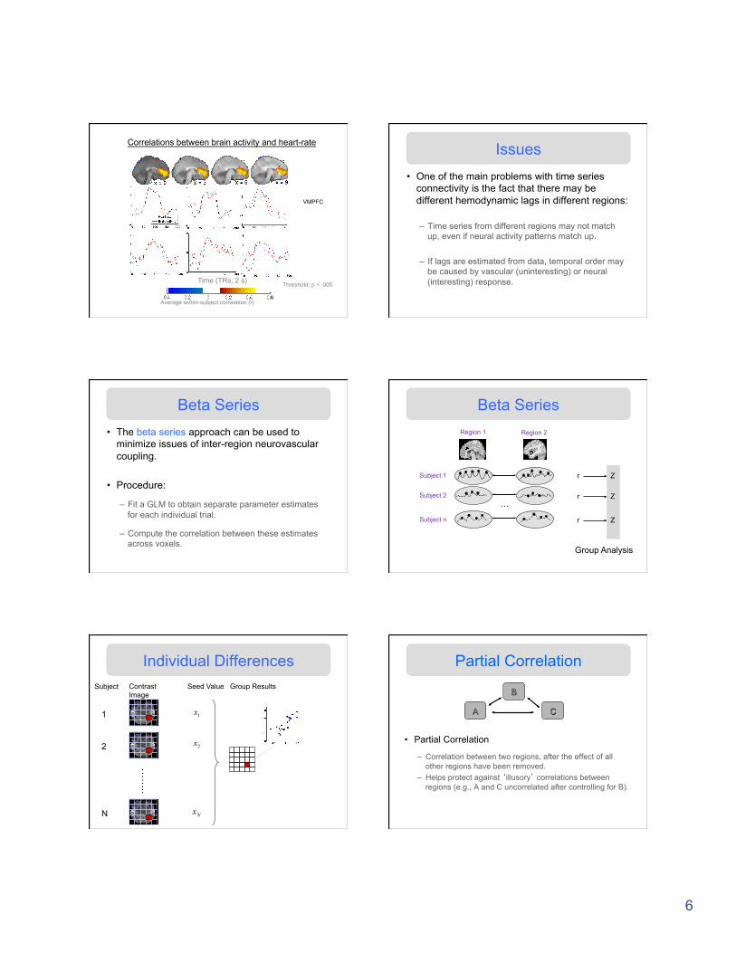
Correlations between brain activity and heart-rate

Time (TRs, 2 s)

Average within-subject correlation (r)

Threshold: p < .005

VMPFC

Issues •  One of the main problems with time series

connectivity is the fact that there may be different hemodynamic lags in different regions:

–  Time series from different regions may not match up, even if neural activity patterns match up.

–  If lags are estimated from data, temporal order may be caused by vascular (uninteresting) or neural (interesting) response.

Beta Series •  The beta series approach can be used to

minimize issues of inter-region neurovascular coupling.

•  Procedure:

–  Fit a GLM to obtain separate parameter estimates for each individual trial.

–  Compute the correlation between these estimates across voxels.

Beta Series Region 1 Region 2

Subject 1

Subject 2

Subject n

…

Group Analysis

r Z

r Z

r Z

Individual Differences

……

..

Subject Contrast Image

1

2

N

Seed Value

1x

2x

Nx

Group Results

Partial Correlation

•  Partial Correlation

–  Correlation between two regions, after the effect of all other regions have been removed.

–  Helps protect against ‘illusory’ correlations between regions (e.g., A and C uncorrelated after controlling for B).

A C

B

7

Inverse Covariance Methods •  For multivariate normal data there exists a duality

between the inverse covariance (precision) matrix and the graph representing relationships between regions.

–  Conditional independence between variables (regions) corresponds to zero entries in the precision matrix.

–  Graphical lasso (GLASSO) can be used to estimate sparse precision matrices and graphs.

A C

B 0

0 =Σ−1

Mediation

•  Mediation –  The relationship between regions A and B is mediated by M –  Can identify functional pathways spanning > 2 regions –  Can be performed on time series data within a subject, or

individual differences (contrast maps, one per subject)

–  Also: Test of whether task-related activations in B are mediated, or explained, by M.

A B M

Task B M

Demonstrating Mediation

x y

m a b

c’ x y

c

Full model, with mediator Reduced model, without mediator

m = im + ax + em y = iy + bm + c'x + e’y

y = iy’ + cx + ey

Decomposition of Effects •  The mediation framework allows us to

decompose the total effect of x on y as follows:

•  Does m explain some of the x-y relationship?

–  Test c – c’, which is equivalent to significance of the ab product.

–  Sobel test or bootstrap test.

c = c' + ab Total effect = Direct effect + Mediated effect

X

M

Y ( )nxxx …,, 21 ( )nyyy …,, 21

( ))(),(),( 21 tmtmtm n…

)(tα )(tβ

Total:

Direct: 'γ

γ

)()()( , txttm miii εα +=

)(')()( ,0

txdssmsy yii

T

ii εγα ++= ∫

)(, txy xiii εγ +=

∫+=T

dsss0

)()(' βαγγ

Functional Mediation Pain Data

α pathway function

Temp Rating

Brain Response

αβ pathway function

β pathway function

Activation in the right anterior insula mediates the relationship between temperature and pain rating.

The key time interval driving the mediation is between 14-24 seconds following activation.

8

Moderation

•  Moderation –  The relationship between regions A and B is moderated by M –  Connectivity between A and B depends on state (level) of M –  Can be performed on time series data within a subject, or

individual differences (contrast maps, one per subject) –  M can be task state or other variable

•  In SPM, on time series data: “Psychophysiological interaction” (PPI).

M

B

A •  In the psychophysiological interaction (PPI) approach, the standard GLM model is supplemented with additional regressors that model the interaction between the task and the time course in a seed region.

εββββ ++++= XRRXY *3210

Task

Time course from seed region

Interaction term

PPI

•  PPI can be used to determine whether the correlation between two brain areas is altered by different psychological contexts.

•  The interaction term reflects the modulation of the slope of the linear relationship with the seed voxel depending on the variable used to create the interaction.

PPI Decomposition Methods •  We often use multivariate decomposition

methods to study functional connectivity. –  Provides a decomposition of the data into separate

components. –  Can be used to find coherent brain networks. –  Provides information on how different brain regions

interact with one another.

•  The most common decomposition methods are principal components analysis and independent components analysis.

Voxels

Tim

e

X

•  Throughout we organize the fMRI data in a T×N matrix X. –  The row dimension is the number of time points and

the column dimension the number of voxels.

Data Organization Principal Components Analysis

•  Principal components analysis involves finding spatial modes, or eigenimages, in the data. –  These are the patterns that account for most of the

variance-covariance structure in the data. –  They are ranked in order of the amount of variation they

explain.

•  The eigenimages can be obtained using singular value decomposition (SVD), which decomposes the data into two sets of orthogonal vectors that correspond to patterns in space and time.

9

Using SVD, we can decompose the matrix X as:

TUSVX =

where U and V are unitary orthogonal matrices and S is a diagonal matrix consisting of ranked singular values.

Each column of V defines a distributed brain region that can be displayed as an image (eigenimages).

Each column of U correspond to the time-dependent profiles associated with each eigenimage.

TUSVX =

Voxels

Tim

e

=

Eigenimages Time courses

TNNN

TT sss vuvuvuX +++= …222111

APPROX. OF Y

s1 + APPROX. OF Y

s2 + ... = u1

v1T

u2

v2T

Worsley

Independent Components Analysis

•  Independent Components Analysis (ICA) is a family of techniques used to extract independent signals from some source signal.

•  ICA provides a method to blindly separate the data into spatially independent components.

•  The key assumption is that the data set consists of p spatially independent components, which are linearly mixed and spatially fixed.

Two people are talking simultaneously in a room with two microphones.

Cocktail Party Problem

Speakers: s1(t) and s2(t). Microphones: x1(t) and x2(t)

)()()()()()(

2221212

2121111

tsatsatxtsatsatx

+=

+= ASX =→

Mixing matrix Source matrix

10

Assumptions

•  If the mixing matrix is known, the problem is straight forward.

•  However, ICA solves this problem without knowing the mixing parameters.

•  Instead it exploits some key assumptions:

–  Linear mixing of sources.

–  The components si are statistically independent.

–  The components si are non-Gaussian.

ICA Estimation

•  We can find the independent components using a variety of different approaches. –  Maximizing non-Gaussianity –  Minimizing the mutual information –  Maximum likelihood estimation –  Projection pursuit

ICA for fMRI

•  It is assumed that the fMRI data can be modeled by identifying sets of voxels whose activity both vary together over time and are different from the activity in other sets.

•  Decompose the data set into a set of spatially independent component maps with a set of corresponding time-courses.

ICA for fMRI

+

A[ ]1 2Ts s=s

fMRI data

fMRI data is assumed to be a linear mixture of statistically independent sources, s.

×

×

Source 1

Source 2

Time course 1

Time course 2 Vince Calhoun

×

×

ICA for fMRI

•  We seek to decompose X as follows:

where the matrix S contains statistically independent maps in its rows each with an internally consistent time-course contained in the associated column of the mixing matrix A.

ASX =

Voxels

Tim

e

=

Mixing Matrix

Components Data

Spatially independent Components

Time Courses

ASX =

Use an ICA algorithm to find A and S.

Overview

11

Comments •  Unlike PCA which assumes an orthonormality

constraint, ICA assumes statistical independence among a collection of spatial patterns.

•  Independence is a stronger requirement than orthonormality.

•  However, in ICA the spatially independent components are not ranked in order of importance as they are when performing PCA.

Types of ICA •  An ICA that decomposes the original data into

spatially statistically independent components is called spatial ICA (sICA).

•  It is possible to switch the order and make the temporal dynamics independent. This is called temporal ICA (tICA).

•  Spatial ICA is more common in fMRI data analysis.

McKeown, et. al.

Multi-subject Analysis •  Using ICA to analyze fMRI data from multiple

subjects raises several questions. –  How should components be combined across subjects? –  How should the final results be thresholded and/or presented?

•  There are several approaches: –  Stack time courses (forces time courses to be the same) –  Stack images and back-reconstruct (allows time courses to

vary, allows some flexibility in images) –  Stack into a cube (forces images and time courses to be the

same)

Group ICA •  Group ICA is based on temporal concatenation.

•  It decomposes the group matrix, and estimates through back-reconstruction the spatial weights for each subject for a component of interest.

•  For each subject the spatial weights at each voxel are treated as random variables, and a t-test is used to test whether that voxel loaded significantly on that component in the group.

Group ICA

X

Subject 1

Subject N

Data

A S_agg

ICA

A1

AN

= ×

Subject i

Back-reconstruction

×1−

=Ai Si

= ×

× = -1