statistical methods in analytical measurements using … · why statistics? • 3 types of lies?...

Statistical Methods in Analytical

Measurements Using ICP

Dr. Lesley S. Owens

Why Statistics?

• 3 types of lies?

– “lies, damned lies, and statistics” – Benjamin Disraeli (British Prime Minister)

• Generate more than one data point for each analysis

• Uncertainty in every measurement

• Learn from and interpret data

Key Topics

• Definitions

• Gaussian Distributions

• Confidence Intervals

• Data Comparisons

• Regression

• Limits

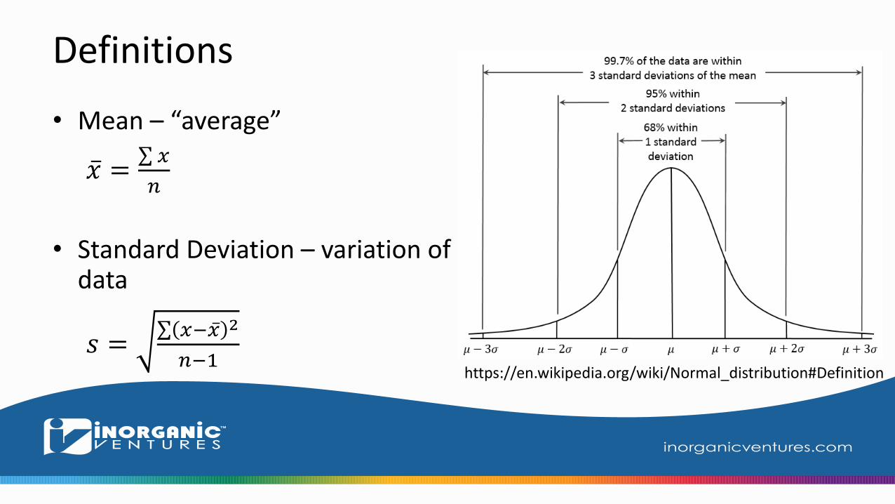
Definitions

• Mean – “average”

𝑥 = 𝑥

𝑛

• Standard Deviation – variation of data

𝑠 = 𝑥− 𝑥 2

𝑛−1https://en.wikipedia.org/wiki/Normal_distribution#Definition

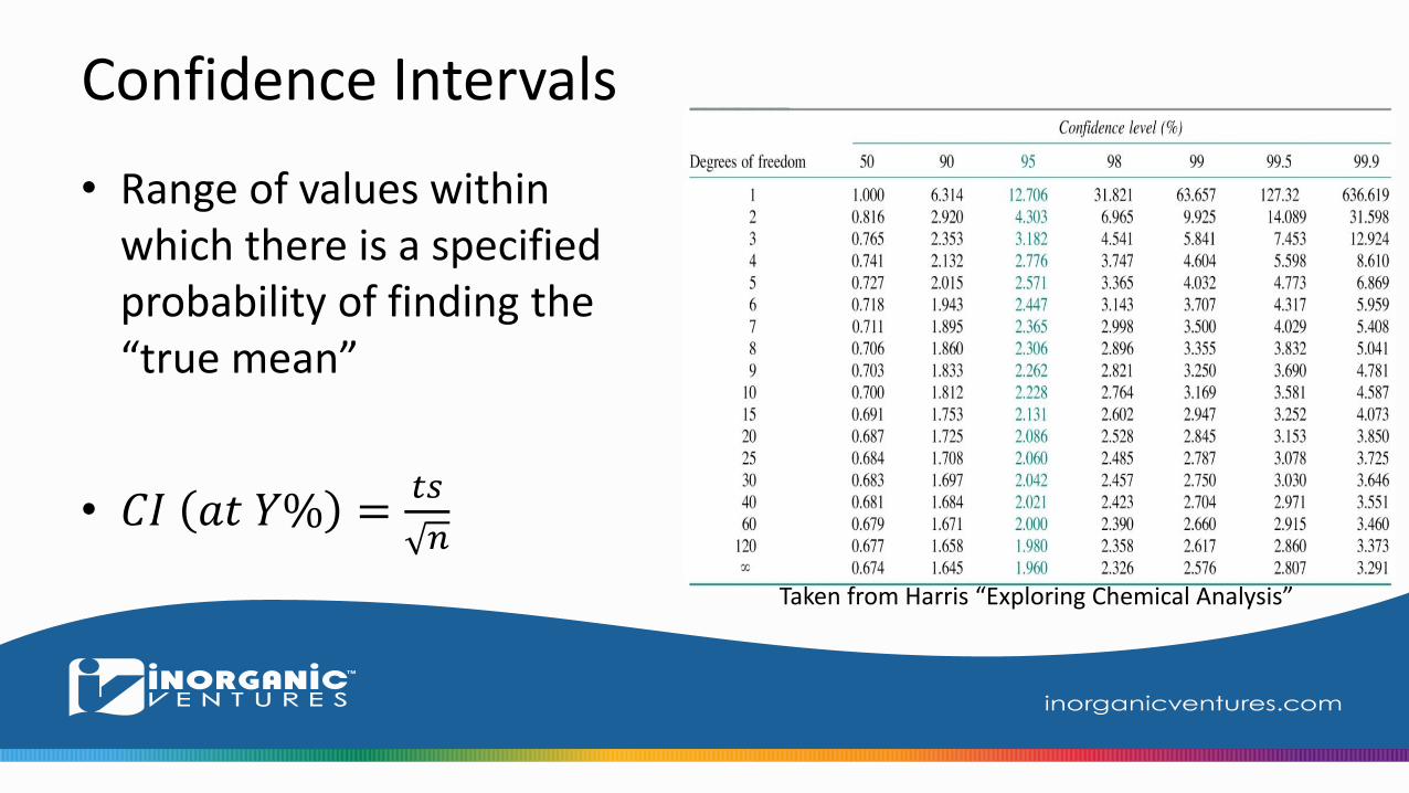
Confidence Intervals

• Range of values within which there is a specified probability of finding the “true mean”

• 𝐶𝐼 𝑎𝑡 𝑌% =𝑡𝑠

𝑛

Taken from Harris “Exploring Chemical Analysis”

Example

Mean 10.067 ppm

Standard deviation 0.008 ppm

Observations 5

t-table 2.776

𝐶𝐼 @ 95% =𝑡𝑠

𝑛=2.776 ∗ 0.008

5= 0.009932

Result:

10.067 ± 0.010 𝑝𝑝𝑚

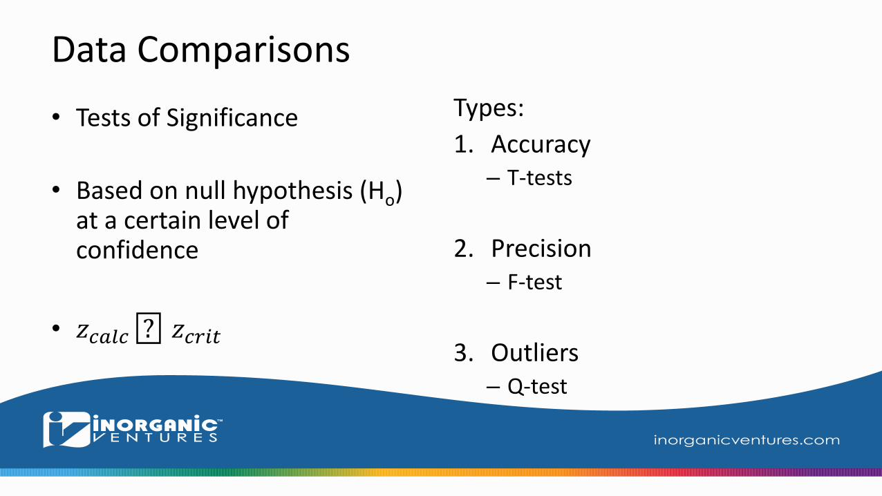
Data Comparisons

• Tests of Significance

• Based on null hypothesis (Ho) at a certain level of confidence

• 𝑧𝑐𝑎𝑙𝑐 ? 𝑧𝑐𝑟𝑖𝑡

Types:

1. Accuracy– T-tests

2. Precision– F-test

3. Outliers– Q-test

T-tests

• Form 1: 𝑥 𝑣𝑠 𝜇

• Form 2: 𝑥1𝑣𝑠 𝑥2

• Form 3: Paired Data

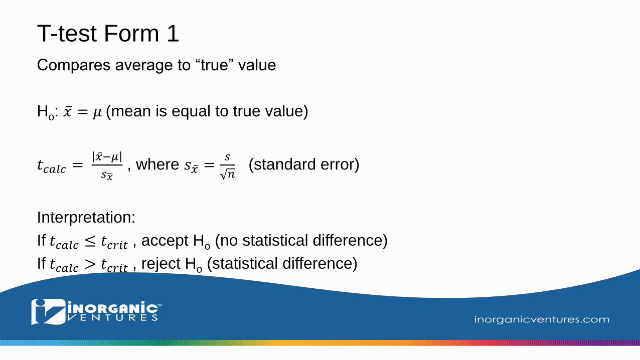
T-test Form 1

Compares average to “true” value

Ho: 𝑥 = 𝜇 (mean is equal to true value)

𝑡𝑐𝑎𝑙𝑐 = 𝑥−𝜇

𝑠 𝑥, where 𝑠 𝑥 =

𝑠

𝑛(standard error)

Interpretation:

If 𝑡𝑐𝑎𝑙𝑐 ≤ 𝑡𝑐𝑟𝑖𝑡 , accept Ho (no statistical difference)

If 𝑡𝑐𝑎𝑙𝑐 > 𝑡𝑐𝑟𝑖𝑡 , reject Ho (statistical difference)

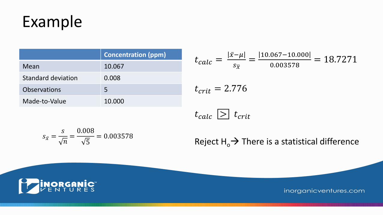
Example

Concentration (ppm)

Mean 10.067

Standard deviation 0.008

Observations 5

Made-to-Value 10.000

𝑡𝑐𝑎𝑙𝑐 = 𝑥−𝜇

𝑠 𝑥=10.067−10.000

0.003578= 18.7271

𝑡𝑐𝑟𝑖𝑡 = 2.776

𝑡𝑐𝑎𝑙𝑐 > 𝑡𝑐𝑟𝑖𝑡

Reject Ho There is a statistical difference 𝑠 𝑥 =𝑠

𝑛=0.008

5= 0.003578

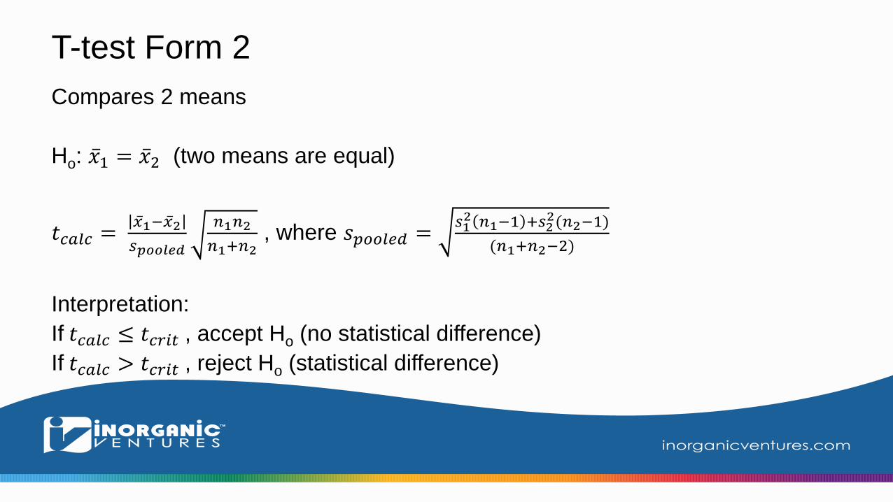
T-test Form 2

Compares 2 means

Ho: 𝑥1 = 𝑥2 (two means are equal)

𝑡𝑐𝑎𝑙𝑐 = 𝑥1− 𝑥2

𝑠𝑝𝑜𝑜𝑙𝑒𝑑

𝑛1𝑛2

𝑛1+𝑛2, where 𝑠𝑝𝑜𝑜𝑙𝑒𝑑 =

𝑠12 𝑛1−1 +𝑠2

2(𝑛2−1)

(𝑛1+𝑛2−2)

Interpretation:



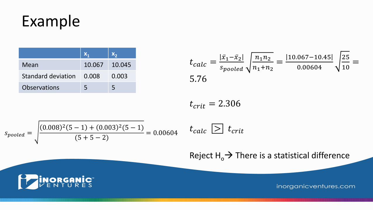
Example

x1 x2

Mean 10.067 10.045

Standard deviation 0.008 0.003

Observations 5 5

𝑡𝑐𝑎𝑙𝑐 = 𝑥1− 𝑥2

𝑠𝑝𝑜𝑜𝑙𝑒𝑑

𝑛1𝑛2

𝑛1+𝑛2=10.067−10.45

0.00604

25

10=

5.76

𝑡𝑐𝑟𝑖𝑡 = 2.306

𝑡𝑐𝑎𝑙𝑐 > 𝑡𝑐𝑟𝑖𝑡

Reject Ho There is a statistical difference

𝑠𝑝𝑜𝑜𝑙𝑒𝑑 =0.008 2 5 − 1 + 0.003 2(5 − 1)

(5 + 5 − 2)= 0.00604

T-test Form 3

Compares paired data

Ho: 𝐷 = 0 (hypothesized mean difference is equal to 0)

𝑡𝑐𝑎𝑙𝑐 = 𝑑− 𝐷

𝑠 𝑑, where 𝑑 = 𝑥1 − 𝑥2 and 𝑠 𝑑 =

𝑠𝑑

𝑛

Interpretation:



Example Before(ppm)

After(ppm)

Difference (ppm)

15.3 7.2 8.1

12.1 8.9 3.2

16.4 8.7 7.7

10.5 9.1 1.4

average 13.6 8.5 5.1

stdev 3.4

𝑡𝑐𝑎𝑙𝑐 = 𝑑− 𝐷

𝑠 𝑑=5.1−0

3.4 4= 3

𝑡𝑐𝑟𝑖𝑡 = 3.182

𝑡𝑐𝑎𝑙𝑐 < 𝑡𝑐𝑟𝑖𝑡

Accept Ho There is a no statistical difference

𝑠 𝑥 =𝑠

𝑛=0.008

5= 0.003578

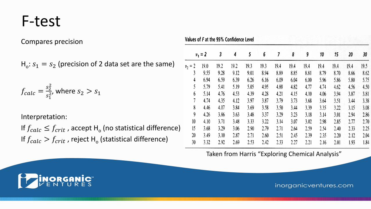
F-testCompares precision

Ho: 𝑠1 = 𝑠2 (precision of 2 data set are the same)

𝑓𝑐𝑎𝑙𝑐 =𝑠22

𝑠12, where 𝑠2 > 𝑠1

Interpretation:

If 𝑓𝑐𝑎𝑙𝑐 ≤ 𝑓𝑐𝑟𝑖𝑡 , accept Ho (no statistical difference)

If 𝑓𝑐𝑎𝑙𝑐 > 𝑓𝑐𝑟𝑖𝑡 , reject Ho (statistical difference)


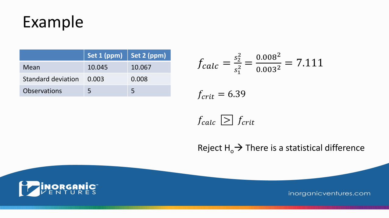
Example

Set 1 (ppm) Set 2 (ppm)

Mean 10.045 10.067

Standard deviation 0.003 0.008

Observations 5 5

𝑓𝑐𝑎𝑙𝑐 =𝑠22

𝑠12 =0.0082

0.0032= 7.111

𝑓𝑐𝑟𝑖𝑡 = 6.39

𝑓𝑐𝑎𝑙𝑐 > 𝑓𝑐𝑟𝑖𝑡

Reject Ho There is a statistical difference

Q-testOutliers

Ho: point in question part of data set

𝑄𝑐𝑎𝑙𝑐 =𝑥𝑞−𝑥𝑛

𝑟𝑎𝑛𝑔𝑒, where 𝑥𝑞 is the point in

question and 𝑥𝑛 is the nearest point

Interpretation: If 𝑄𝑐𝑎𝑙𝑐 ≤ 𝑄𝑐𝑟𝑖𝑡 , accept Ho (keep point)If 𝑄𝑐𝑎𝑙𝑐 > 𝑄𝑐𝑟𝑖𝑡 , reject Ho (discard point)

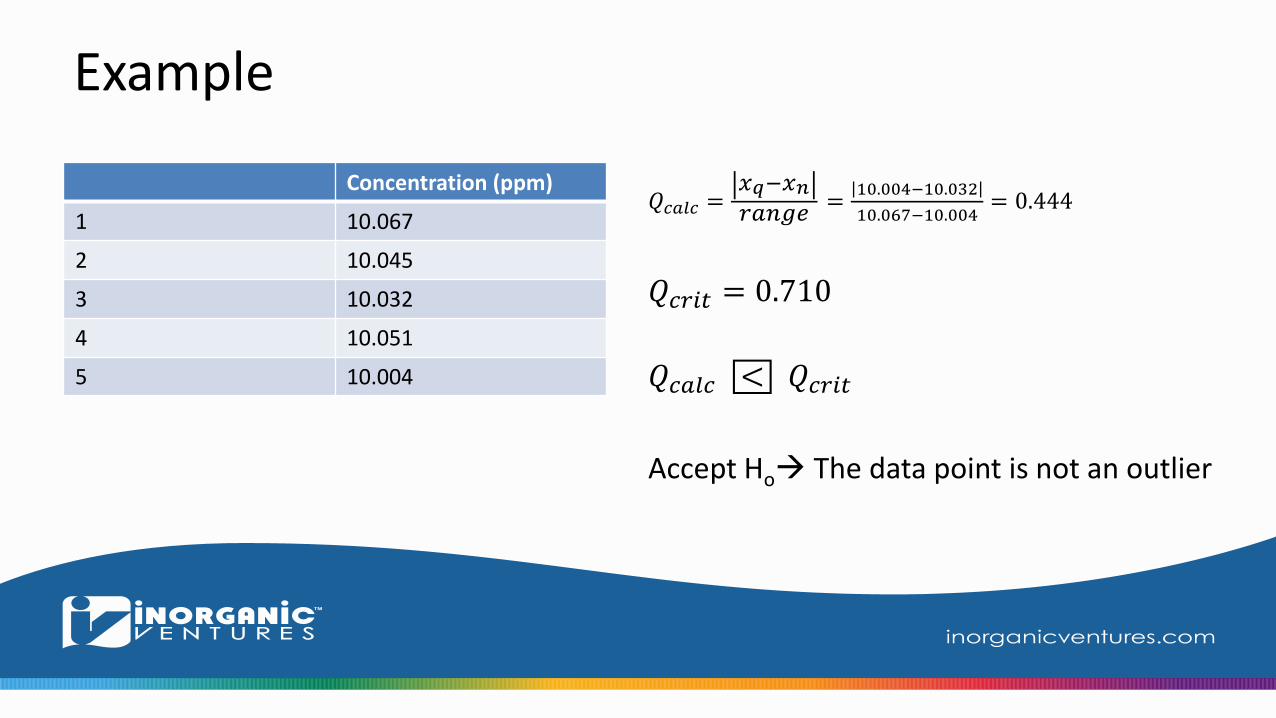
Example

Concentration (ppm)

1 10.067

2 10.045

3 10.032

4 10.051

5 10.004

𝑄𝑐𝑎𝑙𝑐 =𝑥𝑞−𝑥𝑛𝑟𝑎𝑛𝑔𝑒

=10.004−10.032

10.067−10.004= 0.444

𝑄𝑐𝑟𝑖𝑡 = 0.710

𝑄𝑐𝑎𝑙𝑐 < 𝑄𝑐𝑟𝑖𝑡

Accept Ho The data point is not an outlier

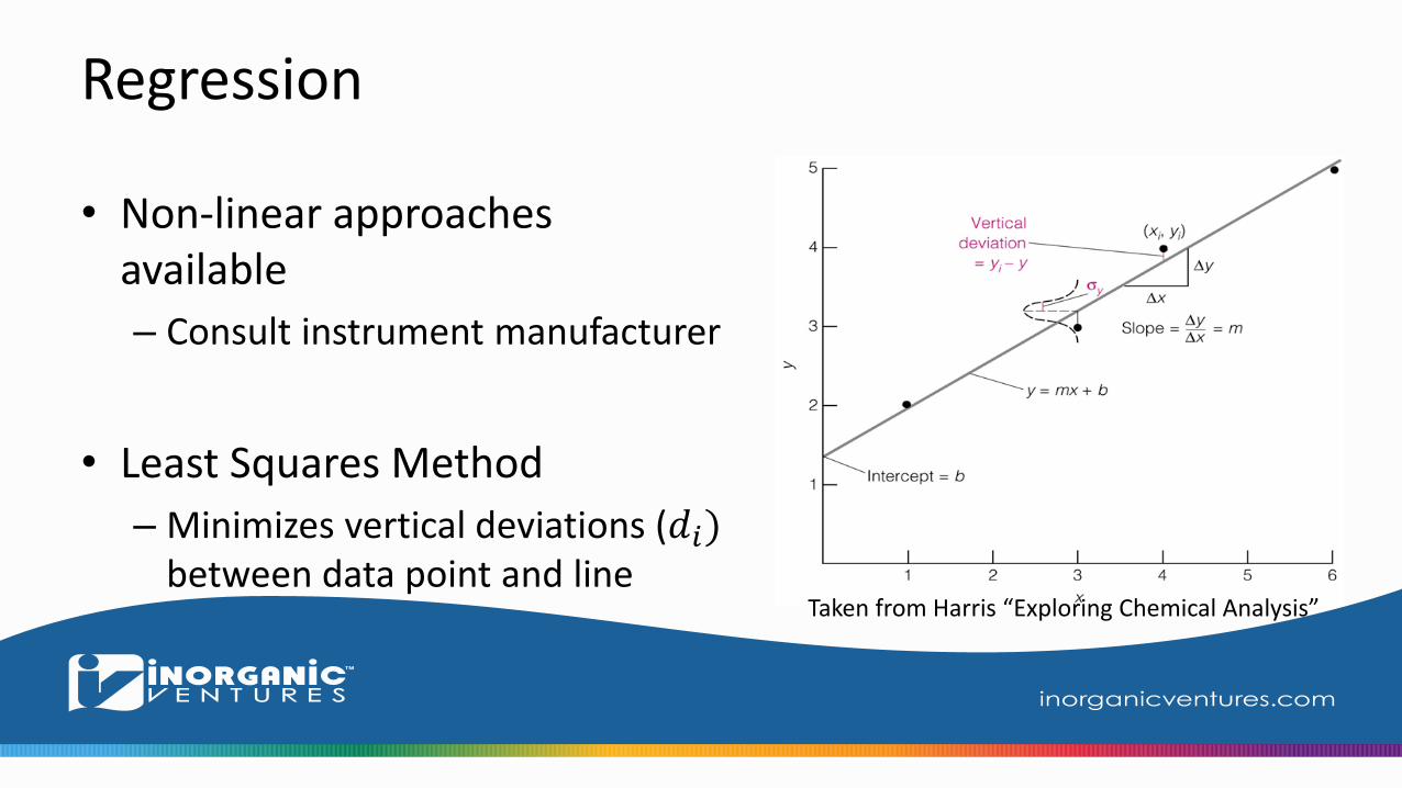
Regression

• Non-linear approaches available

– Consult instrument manufacturer

• Least Squares Method

– Minimizes vertical deviations (𝑑𝑖)between data point and line


Regression Equation

• Vertical Deviation

𝑑𝑖 = 𝑦𝑖 − 𝑦 = 𝑦𝑖 −𝑚𝑥 − 𝑏

• Slope

𝑚 =𝑛 𝑥𝑖𝑦𝑖 − 𝑥𝑖 𝑦𝑖

𝐷, where 𝐷 = 𝑛 𝑥𝑖

2 − 𝑥𝑖2

• Intercept

𝑏 = 𝑥𝑖2 𝑦𝑖 − 𝑥𝑖𝑦𝑖 𝑥𝑖

𝐷


x y

1 2

3 3

4 4

6 5

Regression Example

xi yi xiyi xi2

1 2 2 1

3 3 9 9

4 4 16 16

6 5 30 36

14 14 57 62

𝑚 =𝑛 𝑥𝑖𝑦𝑖 − 𝑥𝑖 𝑦𝑖

𝐷=4 57 − (14)(14)

52= 0.61538

𝐷 = 𝑛 𝑥𝑖2 − 𝑥𝑖

2

= 4 62 − 142 = 52

𝑏 = 𝑥𝑖2 𝑦𝑖 − 𝑥𝑖𝑦𝑖 𝑥𝑖

𝐷=62 14 − 57 14

52= 1.34615

𝑦 = 0.61538𝑥 + 1.34615y = 0.6154x + 1.3462

0

1

2

3

4

5

6

0 1 2 3 4 5 6 7

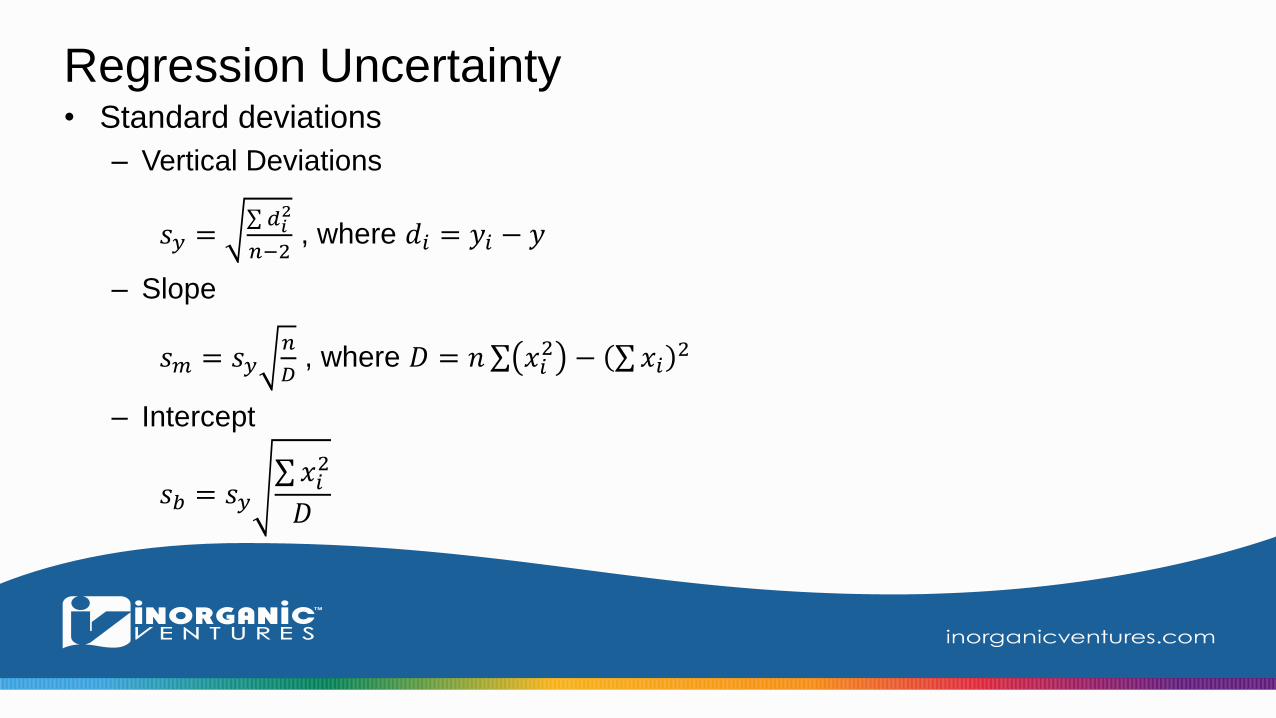
Regression Uncertainty • Standard deviations

– Vertical Deviations

𝑠𝑦 = 𝑑𝑖2

𝑛−2, where 𝑑𝑖 = 𝑦𝑖 − 𝑦

– Slope

𝑠𝑚 = 𝑠𝑦𝑛

𝐷, where 𝐷 = 𝑛 𝑥𝑖

2 − 𝑥𝑖2

– Intercept

𝑠𝑏 = 𝑠𝑦 𝑥𝑖2

𝐷

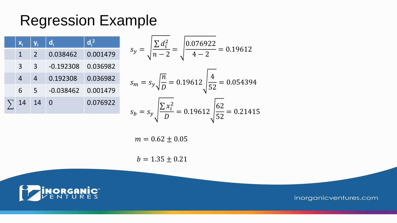
Regression Example

xi yi di di2

1 2 0.038462 0.001479

3 3 -0.192308 0.036982

4 4 0.192308 0.036982

6 5 -0.038462 0.001479

14 14 0 0.076922

𝑠𝑚 = 𝑠𝑦𝑛

𝐷= 0.19612

4

52= 0.054394

𝑠𝑦 = 𝑑𝑖2

𝑛 − 2=0.076922

4 − 2= 0.19612

𝑠𝑏 = 𝑠𝑦 𝑥𝑖2

𝐷= 0.19612

62

52= 0.21415

𝑚 = 0.62 ± 0.05

𝑏 = 1.35 ± 0.21

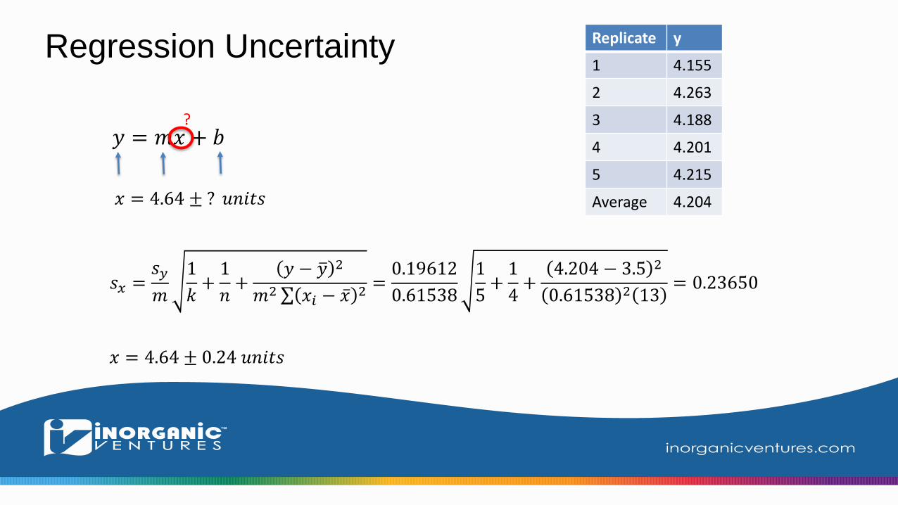
Regression Uncertainty

𝑦 = 𝑚𝑥 + 𝑏

𝑥 = 4.64 ± ? 𝑢𝑛𝑖𝑡𝑠

?

𝑠𝑥 =𝑠𝑦

𝑚

1

𝑘+1

𝑛+𝑦 − 𝑦 2

𝑚2 𝑥𝑖 − 𝑥2=0.19612

0.61538

1

5+1

4+4.204 − 3.5 2

0.61538 2 13= 0.23650

Replicate y

1 4.155

2 4.263

3 4.188

4 4.201

5 4.215

Average 4.204

𝑥 = 4.64 ± 0.24 𝑢𝑛𝑖𝑡𝑠

Limit of Detection (LOD)

• Smallest quantity statistically different from the blank

• <1% chance of blank signal being detected

• 𝐿𝑂𝐷 =3𝑠

𝑚Taken from Harris “Exploring Chemical Analysis”

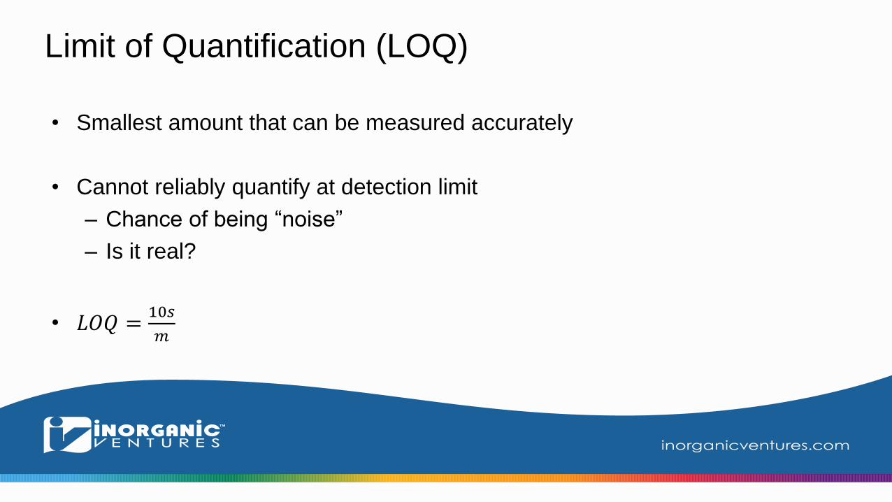
Limit of Quantification (LOQ)

• Smallest amount that can be measured accurately

• Cannot reliably quantify at detection limit

– Chance of being “noise”

– Is it real?

• 𝐿𝑂𝑄 =10𝑠

𝑚

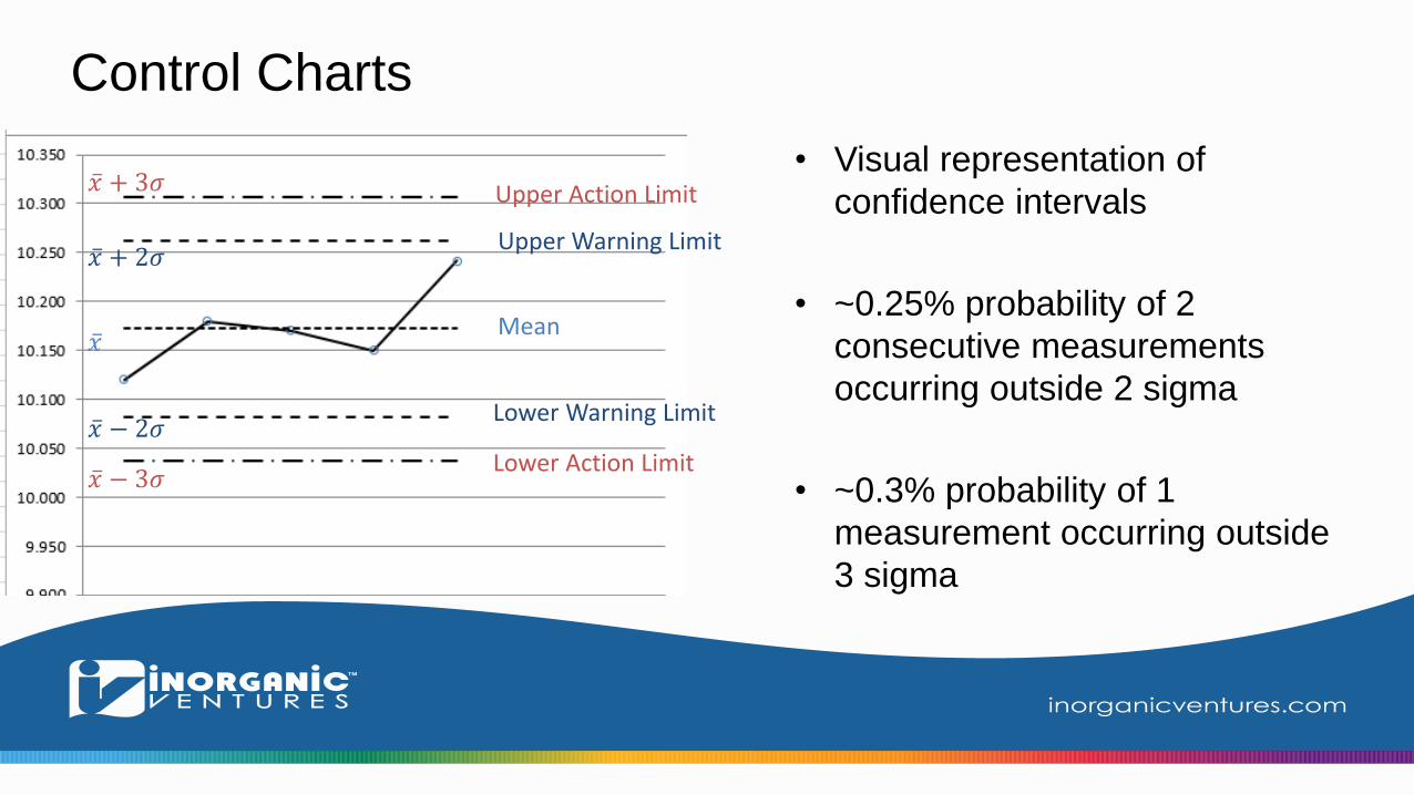
Control Charts

• Visual representation of

confidence intervals

• ~0.25% probability of 2

consecutive measurements

occurring outside 2 sigma

• ~0.3% probability of 1

measurement occurring outside

3 sigma

Mean

Lower Warning Limit

Upper Warning Limit

Lower Action Limit

Upper Action Limit

𝑥 + 2𝜎

𝑥 − 2𝜎

𝑥 + 3𝜎

𝑥 − 3𝜎

𝑥

QUESTIONS?

statistical methods in analytical measurements using … · why statistics? • 3 types of lies?...

Documents