statistical methods for exploring neuronal …
TRANSCRIPT

STATISTICAL METHODS FOR EXPLORING
NEURONAL INTERACTIONS
by
Mengyuan Zhao
B.S. Probability & Statistics, Peking University, Beijing, China 2005
M.A. Statistics, University of Pittsburgh, Pittsburgh, PA 2008
Submitted to the Graduate Faculty of
the Arts & Sciences in partial fulfillment
of the requirements for the degree of
Doctor of Philosophy
University of Pittsburgh
2010

UNIVERSITY OF PITTSBURGH
ARTS & SCIENCES
This dissertation was presented
by
Mengyuan Zhao
It was defended on
June 25, 2010
and approved by
Satish Iyengar, Professor, Statistics
Leon J. Gleser, Professor, Statistics
Robert T. Krafty, Assistant Professor, Statistics
Aaron P. Batista, Assistant Professor, Bioengneering
Dissertation Director: Satish Iyengar, Professor, Statistics
ii

STATISTICAL METHODS FOR EXPLORING NEURONAL
INTERACTIONS
Mengyuan Zhao, PhD
University of Pittsburgh, 2010
Generalized linear models (GLMs) offer a platform for analyzing multi-electrode recordings
of neuronal spiking. We suggest an L1-regularized logistic regression model to detect short-
term interactions under certain experimental setups. We estimate parameters of this model
using a coordinate descent algorithm; we determine the optimal tuning parameter using
BIC, and prove its asymptotic validity. Simulation studies of the method’s performance
show that this model can detect excitatory interactions with high sensitivity and specificity
with reasonably large recordings, even when the magnitude of the interactions is small;
similar results hold for inhibition for sufficiently high baseline firing rates. The method is
somewhat robust to network complexity and partial observation of networks. We apply our
method to multi-electrode recording data from monkey dorsal premotor cortex (PMd). Our
results point to certain features of short-term interactions when a monkey plans a reach.
Next, we propose a variable coefficients GLM model to assess the temporal variation
of interactions across trials. We treat the parameters of interest as functions over trials,
and fit them by penalized splines. There are also nuisance parameters assumed constant,
which are mildly penalized to guarantee the finite maximum of the log-likelihood. We choose
tuning parameters for smoothness by generalized cross validation, and provide simultaneous
confidence bands and hypothesis tests for null models. To achieve efficient computation, some
modifications are also made. We apply our method to a subset of the monkey PMd data.
Before the implementation to the real data, simulations are done to assess the performance
of the proposed model.
iii

Finally, for the logistic and Poisson models, one possible difficulty is that iterative al-
gorithms for estimation may not converge because of certain data configurations (called
complete and quasicomplete separation for the logistic). We show that these features are
likely to occur because of refractory periods of neurons, and show how standard software
deals with this difficulty. For the Poisson model, we show that such difficulties arise possibly
due to bursting or specifics of the binning. We characterize the nonconvergent configura-
tions for both models, show that they can be detected by linear programming methods, and
propose remedies.
iv

TABLE OF CONTENTS
1.0 INTRODUCTION . . . . . . . . . . . . . . . . . . . . . . . . . . . . . . . . . 1
1.1 Multi-electrode recording and neuronal interactions . . . . . . . . . . . . . 1
1.2 Variation of neuronal interactions across trials . . . . . . . . . . . . . . . . 3
1.3 Other statistical issues . . . . . . . . . . . . . . . . . . . . . . . . . . . . . 5
1.4 Organization of this dissertation . . . . . . . . . . . . . . . . . . . . . . . . 7
2.0 EXPERIMENTAL METHODS AND GLM FRAMEWORK . . . . . . 8
2.1 The monkey reach experiments . . . . . . . . . . . . . . . . . . . . . . . . 8
2.2 GLM framework for multi-electrode recording data . . . . . . . . . . . . . 10
3.0 AN L1-REGULARIZED LOGISTICMODEL FORDETECTING SHORT-
TERM NEURONAL INTERACTIONS . . . . . . . . . . . . . . . . . . . 13
3.1 L1-regularized logistic model . . . . . . . . . . . . . . . . . . . . . . . . . . 13
3.2 Coordinate descent algorithm for optimization . . . . . . . . . . . . . . . . 14
3.3 BIC for choosing tuning parameter . . . . . . . . . . . . . . . . . . . . . . 16
3.4 Simulation study . . . . . . . . . . . . . . . . . . . . . . . . . . . . . . . . 18
3.4.1 Simulation setup . . . . . . . . . . . . . . . . . . . . . . . . . . . . . 18
3.4.2 Simulation results . . . . . . . . . . . . . . . . . . . . . . . . . . . . 20
3.4.2.1 Complexity of the network . . . . . . . . . . . . . . . . . . . 20
3.4.2.2 Interaction strength . . . . . . . . . . . . . . . . . . . . . . . 21
3.4.2.3 Size of the Dataset . . . . . . . . . . . . . . . . . . . . . . . 22
3.4.2.4 Excitation and inhibition . . . . . . . . . . . . . . . . . . . . 22
3.4.2.5 Subpopulation . . . . . . . . . . . . . . . . . . . . . . . . . . 23
3.4.3 Conclusion . . . . . . . . . . . . . . . . . . . . . . . . . . . . . . . . 26
v

3.5 Monkey data results . . . . . . . . . . . . . . . . . . . . . . . . . . . . . . 26
3.6 Discussion . . . . . . . . . . . . . . . . . . . . . . . . . . . . . . . . . . . . 33
4.0 A VARIABLE COEFFICIENTS MODEL FOR THE VARIATION OF
NEURONAL INTERACTIONS ACROSS TRIALS . . . . . . . . . . . . 34
4.1 Variable coefficients models . . . . . . . . . . . . . . . . . . . . . . . . . . 34
4.2 GCV, confidence bands and hypothesis testing . . . . . . . . . . . . . . . . 36
4.3 Simulation study . . . . . . . . . . . . . . . . . . . . . . . . . . . . . . . . 39
4.3.1 Single-input network . . . . . . . . . . . . . . . . . . . . . . . . . . . 39
4.3.2 Multiple-input network . . . . . . . . . . . . . . . . . . . . . . . . . 41
4.4 Monkey data results . . . . . . . . . . . . . . . . . . . . . . . . . . . . . . 44
4.5 Discussion . . . . . . . . . . . . . . . . . . . . . . . . . . . . . . . . . . . . 48
5.0 NONCONVERGENCE IN LOGISTIC AND POISSONMODELS FOR
NEURONAL SPIKING . . . . . . . . . . . . . . . . . . . . . . . . . . . . . 54
5.1 The nonconvergence problem . . . . . . . . . . . . . . . . . . . . . . . . . . 54
5.2 Infinite MLE in logistic regression . . . . . . . . . . . . . . . . . . . . . . . 55
5.2.1 Complete and quasi-complete separation . . . . . . . . . . . . . . . . 55
5.2.2 An example . . . . . . . . . . . . . . . . . . . . . . . . . . . . . . . . 57
5.3 The Poisson model . . . . . . . . . . . . . . . . . . . . . . . . . . . . . . . 58
5.4 Remedies . . . . . . . . . . . . . . . . . . . . . . . . . . . . . . . . . . . . 61
6.0 FUTURE WORK . . . . . . . . . . . . . . . . . . . . . . . . . . . . . . . . . 64
6.1 Multi-stage model selection methods in detecting neuronal interactions . . 64
6.2 Error-in-variables methods for tuning curves . . . . . . . . . . . . . . . . . 65
APPENDIX A. PROOF OF THEOREM IN SECTION 3.3 . . . . . . . . . . 70
APPENDIX B. THE EXPRESSIONS OF THE INEXACT GRADIENT
AND HESSIAN OF THE GCV . . . . . . . . . . . . . . . . . . . . . . . . . 73
APPENDIX C. SILVAPULLE’S THEOREM AND INFINITE MLE FOR
SPIKE TRAIN DATA . . . . . . . . . . . . . . . . . . . . . . . . . . . . . . 75
C.1 Silvapulle’s theorem . . . . . . . . . . . . . . . . . . . . . . . . . . . . . . . 75
C.2 Proof of Proposition in Section 5.2.1 . . . . . . . . . . . . . . . . . . . . . 75
APPENDIX D. PROOF OF THEOREM IN SECTION 5.3 . . . . . . . . . . 77
vi

APPENDIX E. INEQUALITY ARRAYS AND LINEAR PROGRAMMING 79
BIBLIOGRAPHY . . . . . . . . . . . . . . . . . . . . . . . . . . . . . . . . . . . . 81
vii

LIST OF TABLES
1 Experimental parameters for the three data sets . . . . . . . . . . . . . . . . 10
2 Sensitivities and specificities for 2 types of network under 3 different |βci1|. The
baseline firing rate is 10 Hz and data length is 5 s. . . . . . . . . . . . . . . . 20
3 Sensitivities and specificities for the two types of network under 3 different
|βci1|. The baseline firing rate is 10 Hz and data length is 25 s. . . . . . . . . 21
4 Sensitivities and specificities for the two types of network under 3 different
|βci1|. The baseline firing rate is 10 Hz and data length is 50 s. . . . . . . . . 22
5 Sensitivities and specificities for different baseline firing rates (BFR). |βci1| is
fixed at 2 and data length is 50 s. . . . . . . . . . . . . . . . . . . . . . . . . 23
6 The hypothesis testing results for the baseline and interactions . . . . . . . . 43
7 The hypothesis testing results for the baseline and interactions of Neuron 9 . 53
viii

LIST OF FIGURES
1 A: the experiment scheme B: the target setup for two tasks . . . . . . . . . . 9
2 The spike sorting scheme: A) aligned snippets, B) two well-isolated neurons . 10
3 Two simulated networks . . . . . . . . . . . . . . . . . . . . . . . . . . . . . . 18
4 Parameters for A) excitation, B) inhibition, and C) refractoriness . . . . . . . 19
5 A: the entire network. B: neurons 25-30 unobserved. C: randomly select 10
neurons unobserved. . . . . . . . . . . . . . . . . . . . . . . . . . . . . . . . . 24
6 A: True and detected interaction matrices and their difference for subpop-
ulation in Figure 5B. B: True and detected interactions matrices and their
difference for subpopulation in Figure 5C. . . . . . . . . . . . . . . . . . . . . 25
7 Interaction matrices for Ham2004. Ordered by numbers of received excitations 27
8 Interaction matrices for Ham2004. Ordered by firing rate contrast . . . . . . 28
9 Interaction matrices for Larry2008 in the delay period. Ordered by numbers
of received excitations . . . . . . . . . . . . . . . . . . . . . . . . . . . . . . . 29
10 Interaction matrices for Larry2008 in the delay period. Ordered by firing rate
contrast . . . . . . . . . . . . . . . . . . . . . . . . . . . . . . . . . . . . . . . 29
11 Interactions on the pin map for Larry2008 in the delay period. . . . . . . . . 30
12 Inhibitory interactions on the pin map for Larry2008 in the delay period. . . 31
13 Interaction matrices for Larry2008 in the pre-cue period. Neurons are in as
the same order as in Figure 9 . . . . . . . . . . . . . . . . . . . . . . . . . . . 31
14 Interaction matrices for Larry2008 in the pre-cue period. Neurons are in as
the same order as in Figure 10 . . . . . . . . . . . . . . . . . . . . . . . . . . 32
15 Interactions on the pin map for Larry2008 in the pre-cue period. . . . . . . . 32
ix

16 The simulated single-input network and the parameter setup . . . . . . . . . 39
17 The fitted curves of the baseline firing rate (left) and the excitatory interaction
(right) with confidence bands . . . . . . . . . . . . . . . . . . . . . . . . . . . 40
18 The neuron with multiple inputs and the parameter setup . . . . . . . . . . . 41
19 The results for the three excitatory interactions . . . . . . . . . . . . . . . . . 42
20 The results for the three inhibitory interactions . . . . . . . . . . . . . . . . . 42
21 The results for A) the baseline, and B) the independence to Neuron Eight . . 43
22 Larry2008, Neuron 38. The network (up) and fitted curves with confidence
bands (bottom) . . . . . . . . . . . . . . . . . . . . . . . . . . . . . . . . . . 45
23 Ham2004, Neuron 14. The network (up) and fitted curves with confidence
bands (bottom). . . . . . . . . . . . . . . . . . . . . . . . . . . . . . . . . . . 47
24 Ham2004, Neuron 9. The network. . . . . . . . . . . . . . . . . . . . . . . . . 48
25 Ham2004, Neuron 9. The fitted curves with confidence bands. . . . . . . . . . 49
26 Ham2004, Neuron 9. All fitted curves in one coordinate. . . . . . . . . . . . . 50
27 Ham2004, Neuron 9 and Neuron 14. All fitted curves in one coordinate. . . . 51
28 The configurations . . . . . . . . . . . . . . . . . . . . . . . . . . . . . . . . . 56
29 Projection can avoid CS/QCS, but miss important information in data . . . . 62
30 (Georgopoulos et al. 1982) A: Spike trains of one neuron in multiple trials
under eight movement directions. B: Tuning curve of the neuron in A. . . . . 66
31 (Cohen and Newsome 2008) A: Behavioral task. B: Scheme for the categoriza-
tion of same-pool and different-pool. . . . . . . . . . . . . . . . . . . . . . . . 67
32 (Cohen and Newsome 2008) A: Histogram of context-dependent differences
in correlation coefficients when ∆PD is either < 135◦ or > 135◦. B: Mean
correlation coefficient as a function of ∆PD during stimulus or target period
for the same-pool or different-pool condition. . . . . . . . . . . . . . . . . . . 68
x

1.0 INTRODUCTION
1.1 MULTI-ELECTRODE RECORDING AND NEURONAL
INTERACTIONS
An important goal in neuroscience is to understand the physiology of the brain and nervous
system of primates when they are engaged in various behavioral tasks. An essential part is the
interactions between neurons in relevant brain areas and their relationship to the behaviors
[8, 23, 43, 19, 52]. Multi-electrode recording systems have made feasible the simultaneous
recording of many neurons, allowing neuroscientists to better study neuronal interactions
under different conditions, even though they need not identify synaptic connections. At the
same time, these recordings present a great challenge to data analysts, in that conventional
procedures are often inadequate to handle the high dimensional data from these experiments.
The commonly used tools by neuroscientists to study neuronal interactions are the cross-
correlation histogram [41] and its variants. These include the joint peri-stimulus time his-
togram (JPSTH) [26], the snowflake plot [42, 16], the normalized JPSTH and the shuffle-
corrected cross-correlogram [1, 7]. However, these methods are commonly used to study two
or three neurons at a time, ignoring the possible contributions of other neurons. In addition,
those graphical methods are histogram-based, so when the bin size is chosen large, they may
not capture short-term interactions.
Brillinger introduced generalized linear models (GLMs) for the analysis of the firing rate
of a neuron as a function of the time since its last spike and spiking history of other neurons
[6]. Although he studied small networks (three neurons), GLMs offer a useful framework
for the analysis of tens, even hundreds of simultaneously recorded neurons. Since then,
much of the work in this area has focused on encoding, which fits a model of neural spiking
1

given observed behavior [37, 55, 32]. The GLM approach has the following advantages: it
can handle all recorded neurons simultaneously; the potential triggers of a spike, such as
spike history, neural ensemble and body kinematics, can be incorporated into the analysis
simultaneously; and the corresponding parameters can be treated as an indication of the
interactions among neurons. Further, GLMs can be again generalized to adapt to point
process [37] or or state-space frameworks [32], where hidden inputs such as ‘common-input’
are modeled as stochastic processes. In addition, the use of GLMs for the encoding stage
has proved successful in decoding body movements from neural activity [24, 55], and bet-
ter than entropy methods in spike prediction of single neurons [56]. Modifications of the
GLM framework were also made. For example, to model a smooth spike-triggered effect,
the parameters are treated as smooth functions of time, instead of a discretization of the
lagged time [30, 38]. This modification sometimes is called ‘Markov interval models’ [30];
alternatively, Stevenson et al. [52] added a L2 penalization on the difference of the adjacent
parameters, which functions as a penalty on roughness.
Our interest in GLMs in this context is to assess neuronal interactions and their vari-
ations under different behavioral tasks. We interpret the sign of parameters in GLMs as
excitatory (positive), inhibitory (negative) or lack of (zero) interaction, so that a study of
those parameters should provide an estimate of the nature of the true underlying interac-
tions of neurons. Therefore, a sparse model, that is, one with a small portion of variables
in the original model, will be helpful to highlight the most prominent interactions among
all pairs of recorded neurons. In particular, subclusters of neurons that appear to be depen-
dent would then be good candidates for further study to better characterize the nature of
the interactions. One such attempt by Truccolo et al. [55] uses the AIC to select models.
However, it cannot automatically select the best subset among all variables, because it must
compare all candidate models, which is infeasible for large networks. Therefore, unless we
have postulated a network for testing a priori, an automatic model selection approach is
required to find the neural interactions. In addition, standard stepwise variable selection
methods are susceptible to nonconvergence because certain data configurations can lead to
infinite maximum likelihood estimates (MLEs) of an unregularized GLM [65].
The model selection method we consider here is a version of the lasso, specifically an L1-
2

regularized logistic regression model. This approach has been used before in neuroscience,
but with the primary aim of decoding [37, 43]. More recently, Stevenson et al. used a
Bayesian formulation of L1 regularization to detect long-term neuronal interactions [52].
To assess the performance of the proposed method, we also do simulation studies. In
particular, we study its ability to detect nonzero coefficients when varying several important
factors. The simulations help by lending credibility of our findings in monkey data. Guided
by the simulation study, we implement the proposed method to three monkey data sets with
three different recording lengths. These results point to patterns of interactions among the
neurons under different conditions.
1.2 VARIATION OF NEURONAL INTERACTIONS ACROSS TRIALS
The GLM framework mentioned in the previous section is static, that is, the parameters
which encode the neuronal interactions are assumed constant both within one trial of the
experiment and across trials. However, these assumptions need validation. Eden et al. [17]
introduced a dynamic GLM model, where they modeled the parameters as a multivariate
autoregressive process within each trail. Gilson et al. (2009) [27] model the synaptic connec-
tivity via a dynamical system model, and study the steady states for spike-timing-dependent
plasticity.
In a typical multi-electrode recording experiment, for example, a monkey center-out task
for motor control, there are two temporal variables involved. One is the time within a trial,
and the other is the order of trials. Within a trial, the variation of neuronal interactions can
be due to the onset of the stimuli [9] or the plasticity [27]. Those studies mentioned so far are
mainly focused on modeling the neuronal dynamics within a trial, while trials are treated as
independent and identical replicates. However, the independence and identity of the trials
can be compromised by some uncontrolled conditions, such as monkey fatigue, adaptation in
training, or inputs from other brain areas. Furthermore, in some studies, temporal variation
across trials are more likely to happen than the temporal variation within a trial. For
example, in the study of the relationship between the PMd and the reach planning, only a
3

few hundreds milliseconds period in a trial is of interest, and the neuronal connectivity is
likely to be stationary in that very short period. On the other hand, the entire experiment
can last for hours for repeating trials. The assumption that the neuronal interactions are
stationary over hours is suspectable because of the many uncontrolled conditions that might
occur within these hours.
Therefore to account for the variation of the neuronal interactions, we propose a penalized
semi-parametric variable coefficients model. We treat interaction parameters from the GLM
framework as constant within a trial, but varying across trials. The functions of parameters
should be smooth, so they are assumed to be from a function space spanned by a basis
set, and there is a penalty on the roughness. We implement a B-spline here, although no
specific constrains on the choice of the basis is required. In addition, since the refractoriness
of neurons can cause infinite parameter estimates [65], we also add a mild L2 penalty for
nuisance parameters. The model is fitted by penalized regression spline technique introduced
by [62]. The tuning parameters for smoothness are selected via generalized cross validation
(GCV) criteria [15, 62]. Confidence bands for the smooth functions are provided based on a
Bayesian interpretation of penalized spline models [57, 51], where the more appropriate term
in Bayes statistics should be ‘credible bands’. Since the Bayesian credible bands for smooth
functions are found to perform well from a frequentist viewpoint [57, 51], we use the term
‘confidence bands’ instead in this dissertation. Because the confidence bands introduced
by Wahba and Silverman [57, 51] are based on the selected smoothing parameters, Wood
(2006) [62] calls them ‘conditional Bayesian confidence bands’. To further correct the bias
introduced by data, Wood (2006) [62] suggests the ‘unconditional Bayesian confidence bands’
by bootstraping samples of smoothing parameters first. The confidence bands should also be
constructed simultaneously. We follow a method introduced by Ruppert et al. (2003) [47],
where the bootstrap is also used. Finally, we use likelihood ratio test with approximated χ2
distribution to test the null model of stationary interactions, although we are aware of the
fact that it is an incompletely justified method introduced by Hastie and Tibshirani (1990)
and Wood (2006) [28, 62].
Again, to assess our method’s performance, we simulate a neuron with both single-input
and multi-inputs from other neurons. Simulation studies show that the variable parameters
4

capture the simple variation structure of the interactions across trials, such as monotone
or quadratic variations. The confidence bands and hypothesis tests will further support
the existence of variations across trials. Two monkey data sets, among the three data sets
used in interaction detection, will be used again to see whether there are variations in the
interactions that were detected first by L1 regularization.
1.3 OTHER STATISTICAL ISSUES
In the application of the proposed L1-regularized logistic regression model and variable co-
efficients model, some other important statistical issues are concerned in both theory and
computation.
One concerns the possibility of non-convergence in optimizing the logistic regression
log-likelihood without regularization. Nonconvergence in fitting logistic regression was not
reported in papers [37, 55], but it poses challenges in our analysis. We found that, in
the logistic model the nonconvergence is due to a data configuration called ‘quasicomplete
separation’ of the design matrix [2, 50]. Quasicomplete separation is inevitable in spike train
data, because the refractoriness of neurons determines that two firings within a consecutive
milliseconds do not occur. Extending this work on nonconvergence to Poisson models, we
present the necessary and sufficient conditions for the existence of finite MLEs in Poisson
regression. We characterize the nonconvergent configurations for both models, show that
they can be detected by linear programming methods, and discuss possible remedies. In
both spike train data analyses introduced above, the possible nonconvergence is addressed
and appropriate treatments are implemented to remedy this issue.
Second, although the GLM with L1 regularization method sounds appealing in selecting a
sparse model, the efficiency of computation is a serious issue. Due to the non-differentiability
of L1-regularization term, conventional convex optimization algorithms have been modified
and new numerical algorithms have been proposed [18, 39, 46, 53]. However, more recent
research suggests a ‘coordinate descent’ algorithm in optimizing the convex loss function
plus regularization, with logistic regression with L1 regularization as a special case [21,
5

22]. A similar approach was also found by Wu and Lange [64]. This algorithm is simple
to implement but competitive with other well-known procedures in high dimensional lasso
problems [21, 22]. The corresponding R package, glmnet, which we implemented in model
fitting, is available on the web: http://cran.r-project.org/.
Third, since we do not have enough physiological facts to validate the detected inter-
actions, the theoretical properties of the L1-regularized logistic regression model become
important. The asymptotic properties of both the lasso in model selection [20, 66, 59] and
the BIC in tuning parameters selection [68, 58] are widely studied. Here we synthesize those
results to prove the validity of the proposed L1-regularized logistic model with BIC to select
tuning parameters.
And fourth, several computational issues arose in the variable coefficients model appli-
cations too. First, we may have tens to hundreds of neurons recorded, so that there are at
least tens or hundreds of smooth functions needed to fit, which is computationally inten-
sive. This effort can be reduced by doing the detection of interactions first. From results in
Stevenson et al. [52] and our interaction detection studies, neuronal interactions are found to
be sparse. So based on the sparse results, we can fit much smaller models instead. Second,
the minimization of GCV will be computationally intensive due to the large size of the ob-
servations (n = 10, 000 ∼ 100, 000). Although the method introduced by Wood (2008) [63]
will calculate the exact gradient and Hessian of the GCV, it involves heavy computation.
On the other hand, his earlier method [61] would be less intensive in computation, but the
suggested QR-decomposition of the design matrix X will be infeasible if X has an extremely
large dimension. To avoid this problem, based on the method in Wood (2004) [61], we use a
computationally efficient way to derive the gradient and Hessian of the GCV. Finally, since
both the point-wise unconditional Bayesian confidence bands and simultaneous confidence
bands required bootstrap samples [62, 47], we combine the two algorithms to reduce the
effort in sampling.
6

1.4 ORGANIZATION OF THIS DISSERTATION
The dissertation mainly consists of three parts:
1. An L1-regularized logistic regression model for detecting neuronal interactions on monkey
reach data
2. A variable coefficients model for the variation of interaction across trials
3. Nonconvergence in logistic and Poisson models for neural spiking
as well as the future work:
1. Multi-stage model selection methods in neuronal interaction detection
2. Error-in-variables methods for tuning curves and spike count correlations
In Chapter 2, we introduce the monkey reach experiments and data used for analysis
(Section 2.1), and the GLM framework for spike train data (Section 2.2). In Chapter 3, we
describe the L1-regularized logistic model for detecting neuronal interactions (Section 3.1).
Computational methods (Section 3.2) and tuning parameter selection (Section 3.3) will be
elaborated. In the end of this chapter are the simulation studies (Section 3.4) and real data
analysis (Section 3.5). In Chapter 4, we describe the variable coefficients model for the
variation of interaction across trials (Section 4.1) and how to determine smooth parameters,
construct confidence bands and test the hypotheses (Section 4.2). The simulation studies and
real data analysis will follow (Section 4.3, 4.4). In Chapter 5, we first generally describe the
nonconvergence issue in GLM modeling (Section 5.1), and then move to the details for both
the logistic (Section 5.2) and Poisson models (Section 5.3). Remedies for the nonconvergence
are also provided (Section 5.4). In the end, the future work will be briefly sketched in Chapter
6.
7

2.0 EXPERIMENTAL METHODS AND GLM FRAMEWORK
2.1 THE MONKEY REACH EXPERIMENTS
The analysis done in this dissertation is involved with data from three experiments performed
by two monkeys named Larry and Ham. The three experiments have the same scheme in a
trial, but with two different reach tasks. In all three experiments, neurons from the dorsal
premotor cortex (PMd) were recorded, due to the role of PMd plays in reach planning [10, 5].
In each experiment, an adult male Rhesus monkey (macaca mulatta) participated. All
experimental procedures were approved by Stanford University’s Institutional Animal Care
and Use Committee. The animal performed either an instructed-delayed center-out (CO) or
reference frame (RF) reach task. The animal was extensively trained to perform the task
before experiments began. The monkey faced a vertically-oriented screen. Each trial began
at a square that indicates the touch point (TP). When the monkey touched the TP, a crossing
fixation point (FP) appeared for the monkey fixating the tracked eye to it. After the monkey
gazed at the FP, the reach target (a second square) appeared, and the monkey is required
to maintain his hand and eye position. Next, the TP and FP were extinguished and ‘go’ cue
appeared. The monkey reached his hand to the target. In sum, one trial consists of four
periods: fixation period (from the start to the finish of eye and hand fixation), pre-cue period
(from the end of fixation to the appearance of the target), delay period (from the appearance
of the target to ‘go’ cue) and reaching period (from ‘go’ cue to the acquire of the target);
See Figure 1A. The length of each period varies in the three different experiments. The
trials, the number of which also varies from three experiments, are repeated with complete
randomization of targets. See Table 1 for details.
The three experiments used two tasks, center-out task and reference frame task, which
8

are different in the placement of the TPs and targets. In the center-out task, the TP is in
the center and eight peripheral targets are equally placed; in reference frame task, the TP
is under ten targets, which are parallel placed in two parallel rows (Figure 1B).
Figure 1: A: the experiment scheme B: the target setup for two tasks
Neural data is recorded using a 96-electrode ‘Utah’ array (Blackrock Microsystems, Salt
Lake City, UT) surgically implanted into the PMd. Implantation was designed to target
cortical layer 5, where neurons that project to the primary motor cortex are located (though
electrode depth could not be confirmed.) After the recording, the spikes are sorted from the
whole voltage traces via the algorithm introduced by Santhanam et al. [48]. The snippets
that are suspected to be action potentials are clipped from the whole voltage traces, and
then they are aligned in the same axis relative to the trough (Figure 2A). The spikes were
automatically identified using a three-step process: noise whitening, dimensionality reduction
via principal components analysis, then a clustering algorithm (Figure 2B). Automatically
identified clusters were then assigned sort qualities by the authors.
To study the changing of neuronal interactions in different conditions, only two condi-
tions, reaches to left and to the right, were chosen for all three experiments. In the meanwhile,
9

Figure 2: The spike sorting scheme: A) aligned snippets, B) two well-isolated neurons
only well-isolated neurons with mean firing rates greater than 3Hz in both conditions were
used in analysis. See Table 1 for details.
Table 1: Experimental parameters for the three data sets
Monkey Task Conditions Period Length (ms) # of neurons # of trials
Ham2005 RF up-left, bottom-right delay 500 18 12, 9
Larry2008 CO left, right pre-cue, delay 300, 300 41 574, 559
Ham2004 CO left, right delay 500 30 145, 146
2.2 GLM FRAMEWORK FOR MULTI-ELECTRODE RECORDING DATA
Multi-electrode recording data are often organized in the form of spike trains: discrete count-
valued time series with each value indicating the number of neuron firings (spikes) within
10

the corresponding time interval. Depending on the type of experiment, the time courses of
extrinsic covariate information, such as stimuli or body kinetics, can also accompany the
spike trains. We suppose that all the spike trains and time courses are aligned onto the same
time axis.
We bin the time axis into T equal segments. Typically T is large enough so that, within
each bin of size ∆, at most one spike per neuron occurs in a cell, leading to binary outcomes;
∆ = 1 millisecond (ms) is often chosen [6, 55]. Large bin sizes that lead to count data are
also used [52]. We denote the spike train within the first t bins of neuron c as N c1:t, the
number of spikes within tth bin of neuron c as ∆N ct , history of all neurons and extrinsic
influences before tth bin as Ht and its conditional firing rate (number of spikes per second)
at bin t as λct , where c = 1, 2, ..., C, the number of neurons identified by the electrodes.
Assuming that the firing rate is constant in the time interval ∆, the distribution of ∆N ct
conditioned on the history is typically considered as either Bernoullli if ∆N ct is binary, or
Poisson if ∆N ct is a count. In Bernoulli case:
P (∆N ct |Ht) = [λct∆]∆N
ct [1− λct∆]1−∆Nc
t ,
and in Poisson case:
P (∆N ct |Ht) =
[λct∆]∆Nct
∆N ct !
eλct∆.
Assuming that the spiking probability of a neuron at time t depends only on the history,
and not on the spiking of other neurons at the same time, the likelihood of all spike trains
is:
P (N1:C1:T ) =
C∏c=1
T∏t=1
P (∆N ct |Ht).
Further, if the experiment is repeated J times, we assume that the trials are independent
replicates, so the likelihood is
P (N1:C1:K(1), ..., N1:C
1:T (J)) =J∏j=1
C∏c=1
T∏t=1
P (∆N ct (j)|Ht). (2.1)
Next, we model the conditional firing rate, incorporating all covariates of interest:
g(λct∆) = βc +P∑p=1
βcp∆Nct−p +
∑i 6=c
Q∑q=1
βciq∆Nit−q + I(αc), (2.2)
11

where g is any appropriate link function satisfying the standard requirements of a logistic or
Poisson model, such as the logit or log, respectively [34]. The first term βc in (2.2) denotes
the baseline firing rate. The second term models the effect of the the spiking history effect
of neuron c, with the coefficient βcp indicating the magnitude of effect at lag p, up to a P∆
ms lag. The third term captures neural ensemble effects, with βciq being the magnitude
of effect of neuron i on neuron c at lag q, this time up to a Q∆ ms lag. The last term I
denotes a function, linear in parameters α, of extrinsic covariate effects. For example, to
model the relationship between neuronal activity and monkey hand movement, I may follow
the velocity model [36, 55]:
I(α) = α1|Vt+τ | cos(φt+τ ) + α2|Vt+τ | sin(φt+τ ),
where |V | and φ are hand movement speed and direction, respectively, and τ is the time lag
between the neuronal activity and its consequent effect on movement.
To model the spike history and neural ensemble effects, the covariates ∆N ct−p, ∆N i
t−q
in (2.2) can be substituted by N c1:t−(p−1)W − N c
1:t−pW and N i1:t−(q−1)W − N i
1:t−qW , where W
represents a multiple of ∆. This substitution is equivalent to constraining the βcp and βciq to
be constant in a larger time interval compared to ∆, so that the corresponding spike event
has a persistent effect.
12

3.0 AN L1-REGULARIZED LOGISTIC MODEL FOR DETECTING
SHORT-TERM NEURONAL INTERACTIONS
3.1 L1-REGULARIZED LOGISTIC MODEL
To capture short-term interactions on the order of 5 ms, we build a model with high time
resolution, with ∆ = 1 ms and Q ≤ 5. Note that the use of a small bin size can enlarge the
data set considerably, particularly when the experiment duration of interest is small, say,
500 ms. When ∆ = 1 ms, each ∆N ct is binary, leading to the logistic regression model:
log
(λct∆
1− λct∆
)= βc +
P∑p=1
βcp∆Nct−p +
∑i 6=c
βci1
(Q∑q=1
∆N it−q
)+ I(αc). (3.1)
The parameter βci1 in (3.1) represents the short-term interaction between neuron c and
i within Q (≤ 5) ms, given the activity of all other neurons: a positive βci1 means that
neuron c will be excited within Q ms after neuron i fires, a negative βci1 means inhibitory
interaction, and zero means lack of interaction from neuron i to neuron c. In the last term, αc
are nuisance parameters for extrinsic effects, which can be conveniently excluded from model
when there are no stimuli or body movements. Note that there is no overlap of parameters
in (3.1) for each c, so the entire logistic model can be solved individually: first collect the
parameters βc, {βcp} and {βci1} into a large vector θc and maximize C individual likelihoods
L(θc, αc) = P (N c1:T (1), ..., N c
1:T (J)) =J∏j=1
T∏t=1
P (∆N ct (j)|Ht). (3.2)
Note, however, that maximizing (3.2) itself will not give zero estimates of the interaction
parameters in general, so we use a selection method by zeroing out some βci1. Tibshirani [53]
introduced the lasso to select variables in the linear model. The theory of this L1-regularized
13

model selection procedure has been studied [20, 18, 68], and it has been implemented widely
[54, 40]. Our approach selects a sparse model by minimizing the C individual L1-regularized
logistic models:
f(θc, αc|γc) = −logP (N c1:T (1), ..., N c
1:T (J)) + γc
(∑p
| βcp | +∑i 6=c
| βci1 |
). (3.3)
The L1-regularization can be also directly added to the whole log-likelihood (2.1). How-
ever, since there is no overlap in the parameters for different neurons, fitting C individual
L1-regularization logistic models leaves more flexibility in the choice of regularization param-
eter γ. In addition, decomposing the entire model into C models can decrease the dimension
of the model, so that computation becomes more efficient.
3.2 COORDINATE DESCENT ALGORITHM FOR OPTIMIZATION
Because the function f in (3.3) does not have the first derivative at βcp = 0 and βci1 =
0, a gradient-based method, like Newton-Raphson method, can not be applied directly.
Hence, there has been considerable effort on numerical optimization of the L1-regularization
problem. Tibshirani [53] offered an algorithm where the regularization term was seen as a
combination of linear constraints; however, it was proven to be computationally inefficient,
because∑p
i=1 |βi| implies 2p linear constraints. Later, methods based on path algorithms
[18, 21, 22, 39, 45, 64] largely improved the computation time and the accuracy of the
estimates. The core steps of these path algorithms are:
1. Start estimating β, the vector of all parameters, without regularization, i.e. γ = 0,
or fully regularized, i.e. γ = γmax such that all parameters of interest have zero esti-
mates. The latter is usually the choice, since the parameters are not estimable without
regularization in many cases.
2. Increase or decrease the γ by ∆γ and update the estimate of β(γ+∆γ) from the estimate
of β(γ). It is achievable because at γ = 0, β = βMLE and at γ = γmax, β = 0, so we
have starting points for this iterative algorithm.
14

3. Stop when γ = γmax or γ = 0.
The difference between various path algorithms is in how γ and β are updated, which
determines the complexity and efficiency of the algorithm.
Among these methods, the coordinate descent algorithm [21, 22, 64] has been known for
a long time but neglected. Recently it has recaptured researchers’ attention because of its
computational efficiency as well as its simple implementation in linear and logistic regression.
In addition, the coordinate descent algorithm is not specialized for log-likelihood function
with L1 regularization, but can apply to more general cases, like LAD-lasso, fused lasso and
elastic net [21, 22, 64].
The algorithm takes advantage of the ease in solving single-parameter lasso problems.
Suppose we fit a weighted linear regression model with only one predictor xβ and L1 regu-
larization γ|β|. Thus we minimize
f(β) =1
2
n∑i=1
wi(yi − xiβ)2 + γ|β|. (3.4)
If β > 0, noting that the MLE without regularization is β =∑
iwixiyi/∑
iwix2i , we can
differentiate (3.4) to get
df
dβ=
n∑i=1
wi(yi − xiβ)(−xi) + γ
= (n∑i=1
wix2i )β −
n∑i=1
wixiyi + γ
= (n∑i=1
wix2i )(β − β) + γ
This leads to the analytical solution β = β − γ/∑
iwix2i as long as β − γ/
∑iwix
2i > 0.
Similarly, the solution when β < 0 is β = β + γ/∑
iwix2i with β + γ/
∑iwix
2i < 0. In all,
the analytical form of the lasso estimate βl at γ is:
βl(γ) = S(β, γ) ≡
β − γ/
∑iwix
2i , if β > 0 and γ < |β|
β + γ/∑
iwix2i , if β < 0 and γ < |β|
0, if γ ≥ |β|
(3.5)
15

If we have more than one predictor, we can estimate βj independently, assuming other
β′s (≡ β(j)) are known and fixed. Then the response is no longer yi but the partial residual
rji = yi −∑
k 6=j xikβk. Using (3.5) directly we get the estimate βj(γ|β(j)). Therefore, after
estimating βj, we move to the next parameter, so β can be iterated to convergence. After
we finish the estimation at γ, we increase (or decrease, depending on where you start) γ by
∆γ to estimate βl(γ + ∆γ), for which β
l(γ) can be used as the initial value to speed up the
convergence.
The algorithm above is for linear regression, so adaptation is needed for logistic regression
with L1 regularization. Recalling the iterative reweighted least square (IRLS) estimation for
generalized linear models [34], the coordinate descent algorithm can be embedded within
each iteration of fitting weighted linear regression problems [22]. Here is the adaptation:
• OUTER LOOP: Increase (or decrease) γ.
• MIDDLE LOOP: Update the weights and pseudo-values in the current weighted linear
regression until β or the regularized log-likelihood converge.
• INNER LOOP: Use coordinate descent algorithm to fit the current regularized weighted
linear regression until β converges.
The merit of the coordinate descent algorithm lies in its simple implementation (in each
loop only additions and subtractions) and speed when there are a large number of parameters
[21]. Since βl(γmax) = 0, and when ∆γ is small enough, the difference between β
l(γ) and
βl(γ + ∆γ) is tiny, the convergence should be fast [18, 21, 22, 39, 45].
3.3 BIC FOR CHOOSING TUNING PARAMETER
In addition to minimizing (3.3) under different γ, we need to decide how to choose the
optimal value of γ. There are several commonly used procedures, such as ‘BIC γ-selector’,
‘AIC γ-selector’ or cross validation. Here we call the ‘BIC γ-selector’ or ‘AIC γ-selector’
to distinguish them from the traditional BIC and AIC methods. BIC γ-selector is the one
considered in our analysis. First, it saves time in computation, compared to the extra model
16

fits required by cross validation. Moreover, the BIC as a method to select tuning parameter
has been studied, and it is proven to be consistent in model selection [68, 58]. In our case, the
large sample will not be an issue, and there is additional support from the simulation studies
below. BIC γ-selector chooses the tuning parameter γ which gives smallest BIC value:
BIC(γ) = −2logL(β(γ)) + log(n)×#{nonzero parameters},
where β(γ) is the L1-regularized estimate of parameters for the tuning parameter γ.
All the theoretical studies that we are aware of about consistency of the BIC γ-selector
in model selection are for linear models with various types of regularization [68, 58, 44].
Nevertheless, the asymptotic results of BIC γ-selector in L1-regularized logistic models can
be derived based on those existing theorems. Let us call the models containing all the
covariates with non-zero parameters as ‘correct models’, the model containing all but only
the covariates with non-zero parameters as the ‘true model’, and models missing at least one
covariate with non-zero parameter as ‘wrong models’. Based on some regularity conditions
on link functions, data, and likelihood functions (see Appendix A), we have the following
theorem:
Theorem. For the L1-regularized logistic regression model given in (4) and (5) with a
logit link function, the BIC γ-selector will asymptotically select the correct model with the
smallest number of covariates among all the submodels β(γ) presents.
The Appendix A contains the proof and the details of theorems quoted in my proof.
We will briefly sketch the intuition here. Qian and Wu (2006) [44] showed that, in logistic
regression, the difference of the log-likelihoods between a correct model and the true model
is positive and of order O(log log n). And the difference of the log-likelihoods between the
true model and a wrong model is positive and of order O(n). Therefore, a penalization
of order O(log n), which BIC does, will asymptotically select the true model. Although
BIC(γ) is derived from L1-regularized estimates, the logic described above still holds, as
long as the difference between the L1-regularized log-likelihood of the true model and its
unregularized counterpart is of order o(log n). With regard to that, Theorem 1 in [20] shows
that the L1-regularized estimates can converge with order of o(n−12 log n), and based on
a Taylor expansion, the difference of two log-likelihoods can be controlled to be of order
17

o(log n). Therefore, the BIC γ-selector is consistent in model selection, in the sense that
it asymptotically gives the correct model with smallest number of covariates among all the
submodels β(γ) presents.
3.4 SIMULATION STUDY
3.4.1 Simulation setup
Before we turn to the analysis of the monkey motor cortex experiments, we describe a
simulation study to assess the performance of this L1-regularization logistic model. We
construct two types of network (Figure 3): a simple network consisting of parallel one-way
interactions between pairs of neurons, and a complex one with a hub-and-spoke structure.
Each simulated network will contain 30 neurons. We do not claim that either network is
biologically accurate. Rather, we use them because they do incorporate certain plausible
features such as communication between layers, common input, and recurrent loops. Next,
we choose parameter values to get realistic firing rates.
Figure 3: Two simulated networks
The interactions in the networks will be either excitatory or inhibitory, denoted by posi-
18

tive or negative values on parameter βicq. To simulate the model ,we follow the approach in
Truccolo et al. (2005) [55], with βciq increasing (or decreasing) with q = 1, 2, 3 and βciq = 0
for q > 3 (Figure 4A,B). This choice models short-term dependence: the influence of an
action potential dampens as time passes, with an average duration of 3 ms. On the other
hand, to model refractoriness of a neuron, the spike history parameter βcp should be strongly
negative at the beginning and then rise to a positive value before decreasing to zero: see
Figure 4C. We further require βc to be between −6 and −3 to get a 3Hz-50Hz baseline firing
rate for each neuron. In our illustrations, we set βc = −4.6 to get a 10Hz baseline firing rate,
which is the average firing rate for real neurons.
Figure 4: Parameters for A) excitation, B) inhibition, and C) refractoriness
Here we set Q = 3, P = 60 and C = 30 in model (3.1). Since our focus is mainly on
illustrating the performance on the detection of neuronal interactions, we set I(αc) = 0 to
omit extrinsic effects. Thus, the model becomes:
log(λck∆
1− λck∆) = βc +
60∑p=1
βcp∆Nck−p +
∑i 6=c
βci1(∆N ik−1 + ∆N i
k−2 + ∆N ik−3). (3.6)
We choose this model setup because of our interest in detecting excitatory and inhibitory
interactions within a 3 ms range, rather than the details of the curves in Figure 4. Thus, we
pool the data within the next 3 ms together, and the parameters βci1 will be estimated by
our proposed L1-regularized logistic model with the BIC γ-selector, which would illustrate
the short-term neuronal interactions.
The performance of the proposed method will be assessed in several ways: the complexity
of the network (simple and complex), the strength of the interaction (|βci1| = 2, 3, 4), the
19

size of the data set (5 s, 25 s, or 50 s recording periods), the type of interaction (excitation
or inhibition), and the subpopulation of neurons (partial network). For each combination
of model parameters, the simulation ran 50 independent replicates. The criteria are the
sensitivities (given in three types) and specificities, which are shown in the Tables 2-4.
3.4.2 Simulation results
We now summarize our main findings, with a focus on sensitivity and specificity for detecting
excitation and inhibition. We vary the network complexity, the interaction strengths, the
size of the data set (or recording time); we also assess the model’s performance when only a
subset of the simulated network is observed.
Table 2: Sensitivities and specificities for 2 types of network under 3 different |βci1|. The
baseline firing rate is 10 Hz and data length is 5 s.
Network |βci1| Sensitivity Specificity
total excitation inhibition
2 0.088 0.165 0 0.9994
Simple 3 0.403 0.755 0 0.9994
4 0.531 0.995 0 0.9994
2 0.1 0.15 0 0.9997
Complex 3 0.583 0.874 0 0.9987
4 0.665 0.996 0.02 0.9934
3.4.2.1 Complexity of the network From the Table 2, 3 and 4, we can see that,
although the complex network gives slightly higher sensitivities, there is no major difference
in sensitivities and specificities between two networks. Therefore, the complexity of the
network may not be an important issue when using proposed method to detect neuronal
interactions.
20

Table 3: Sensitivities and specificities for the two types of network under 3 different |βci1|.
The baseline firing rate is 10 Hz and data length is 25 s.
Network |βci1| Sensitivity Specificity
total excitation inhibition
2 0.423 0.793 0 0.9997
Simple 3 0.533 1 0 0.9998
4 0.533 1 0.008 0.9992
2 0.589 0.881 0.004 0.9993
Complex 3 0.668 1 0.004 0.9993
4 0.679 1 0.036 0.9446
3.4.2.2 Interaction strength Fixing all other conditions, all three types of sensitivity
increase with the strength of neuronal interactions (Table 2,3 and 4). The strength of
neuronal interactions is indicated by the magnitude of βci1. When the data set is small (in 5
s data simulation), this increase is more obvious, especially in sensitivity to excitation. For
example, when βci1 = 2, the proposed method can only detect 15% of excitatory interactions,
but with βci1 = 3, it can detect at least 75 percent of them. In other words, if the excitatory
impulse increases the firing rate of a neuron from 10 Hz to 70 Hz (βci1 = 2), it is not large
enough to detect by our method; but if the firing rate is increased to 170 Hz (βci1 = 3) or
more (350 Hz for βci1 = 4), our method has satisfactory sensitivity.
Although 70 Hz may appear to indicate an active neuron, the transience (only 3 ms)
of the interactions prevents us from detecting this effect with a 5s recording period. The
probability of a spike in the next millisecond is only raised from 0.01 to 0.07. When the data
size is enlarged to 50 s, the excitations from 10 Hz to 70 Hz is more likely to be detected.
Nevertheless, note the increase in the sensitivities with the interaction strengths.
Turning to specificity, we note that although it decreases when βci1 = 4 in complex
network, it is still very high. For example, 0.9934 specificity corresponds to in average 5
false interactions in the entire network. Compared to 99.6% ability to detect the true 30
21

Table 4: Sensitivities and specificities for the two types of network under 3 different |βci1|.
The baseline firing rate is 10 Hz and data length is 50 s.
Network |βci1| Sensitivity Specificity
total excitation inhibition
2 0.528 0.985 0.006 0.9997
Simple 3 0.535 1 0.003 0.9999
4 0.537 1 0.008 0.9997
2 0.675 0.999 0.028 0.9997
Complex 3 0.715 1 0.144 0.9959
4 0.738 1 0.214 0.9477
interactions, it is acceptable.
3.4.2.3 Size of the Dataset From the Table 2, 3, and 4, we can see that more data
yield more power of the proposed model to detect the neuronal interactions. For data of size
no shorter than 25 s, maintaining specificities in a high level, the proposed model can detect
more than 80% of the excitation interactions for both networks, even though the strength of
the interactions is small (βci1 = 2). If the strength of interactions is larger (βci1 = 3 or 4), all
of the excitatory interactions are detected. Also, compared to zero sensitivity in detecting
inhibition for 5 s data, a 50 s data set can detect a few inhibitory interactions (up to 20%,
if the strength is high enough).
3.4.2.4 Excitation and inhibition From Tables 2, 3, and 4 we found that inhibition
is hard to detect compared to excitation. We expect that this difficulty is because for firing
rates that are already low, further inhibition is limited by a floor at zero (e.g., 10 Hz rate
corresponds to 0.01 probability of a spike during a 1 ms bin). To verify this conjecture, we
simulated networks with higher baseline firing rates to show the increase in sensitivity for
inhibition. Table 5 shows the results. Given the same interaction strength and data length,
22

higher baseline firing rate results in higher sensitivity in inhibition.
Table 5: Sensitivities and specificities for different baseline firing rates (BFR). |βci1| is fixed
at 2 and data length is 50 s.
Network BFR Sensitivity Specificity
total excitation inhibition
10Hz 0.528 0.985 0.006 0.9997
Simple 15Hz 0.56 1 0.057 0.9998
25Hz 0.867 1 0.714 0.9406
10Hz 0.675 0.999 0.028 0.9997
Complex 15Hz 0.713 1 0.14 0.9996
25Hz 0.973 1 0.918 0.9325
3.4.2.5 Subpopulation In practice the multi-electrode systems surely record only a
small portion of all neurons involved in the behavior under study, so it is also worth studying
the performance of our proposed method when only partial information of the entire network
is acquired. In the other words, when only spike trains of a subpopulation of neurons are
observed, whether our method can at least detect correct interactions between those observed
subpopulation of neurons. In this simulation study, we do not mimic the real network with
millions of neurons. Instead, we simulate a small network with certain sparse interaction
structure, and then we partially observe neurons. We can consider the missing neurons as
neuron ensembles other than single neurons.
Here we assess our method using two types of subpopulations from the complex network
above. The first one studies the performance when one hub and its related spokes are unob-
served. It maintains the overall structure of the entire network. The second one randomly
selects ten neurons unobserved from the entire network. In that case, the main structure of
the network is further destroyed. See Figure 5 for the two types of subpopulation and the
corresponding networks.
The results are shown in Figure 6. Under either subpopulation case, both the true
23

Figure 5: A: the entire network. B: neurons 25-30 unobserved. C: randomly select 10 neurons
unobserved.
and estimated network matrix are given. The network matrix illustrates the subpopulation
network in Figure 5. All the neurons observed are aligned in order. In the true network
matrix, a binary value in (i, j)th element indicates whether neuron j has an either excitatory
or inhibitory influence to neuron i. In the estimated network matrix, a continuous value
in [0, 1] indicates the percentage that the proposed method detects an interaction over 50
runs. Since we only focus on interactions between distinct neurons, diagonal elements are
meaningless here and left as zero.
From Figure 6, we find that, although only a partial network is observed, the proposed
method is still able to detect the excitatory interactions between observed neurons 100% of
the time, despite the missing of hub neurons and the loss of structure. Inhibition remains
hard to detect (bright pixels in difference matrices). Out of 12 total inhibitions in both
subnetworks, nine are successfully detected in less than 15% of 50 runs, and the other three
are detect in less than 40% of 50 runs. False positives occur, but relatively rarely (gray
pixels in difference matrices). Only 5% (51 out of 1071) lack of interactions are at least once
detected as interactions, and among all these 51 positions where the false positives occur,
68% (35 out of 51) are detected as interactions in less than 10% of 50 runs. However, the
situation of false positives is worse (much brighter gray pixels) for second subpopulation than
that for the first. This may be due to the further difference between the observed population
24

Figure 6: A: True and detected interaction matrices and their difference for subpopulation in
Figure 5B. B: True and detected interactions matrices and their difference for subpopulation
in Figure 5C.
25

and the entire network.
3.4.3 Conclusion
In sum, the L1-regularized logistic model can successfully detect short-term excitatory neu-
ronal interactions, with very high specificity. Inhibition is more difficult to detect for low
baseline firing rates. The increase of the sample size and baseline firing rate will, of course,
raise the detection power. Our simulations indicate that at least 25s data will guarantee the
power of the proposed method, even when the strength of interaction is small.
On the other hand, complexity of the network does not appear to influence the perfor-
mance of the proposed method. And it is also robust to the omission of parts of the active
network; however, it would perform better, if the main structure (e.g., hub-and-spoke) of
the entire network can be retained in the observations. Our analysis of the monkey motor
cortex data below is guided by these findings.
3.5 MONKEY DATA RESULTS
The L1-regularized logistic model is applied to three data sets; see Table 1 in Section 2.1
for details of the experimental setup. We first apply the model to data Ham2005 and see
that neither condition shows interaction between neurons. However, it is not sufficient to
conclude no interaction, because there are only approximately 10 trials in each condition (12
and 9 trials respectively), which results in about in total 5 s recordings of the delay period.
The simulation studies show that in this amount of recordings, the sensitivity is extremely
low (Table 2). Therefore, Ham2005 does not give us much information about interactions
due to the small sample size.
Then we apply the model to Ham2004, where approximately 150 trials, or 75 s recording
in delay period, were used in both conditions. We find interactions in both conditions this
time. Because simulation studies show the high sensitivity in interaction detection for this
amount of recording data, we have confidence in the results. The number of the detected
26

interactions in each condition are about in the same amount (67 and 65), which is 7% of
the total possible pairs. The network is given in the form of interaction matrices: (i, j)th
element indicates whether neuron j has an excitatory (white), inhibitory (black) influence or
lack of interaction (gray) to neuron i. To highlight the difference in interactions between the
two conditions, we permute the neuron orders by either the number of received excitations
(Figure 7), or the contrast of the mean firing rates between the two conditions (Figure 8).
The contrast is calculated by:
contrast =rate left− rate right
min(rate left, rate right)
From Figure 7, there is no obvious difference in the pattern of the networks. There is
no neuron more involved in one condition relative to the other condition. From Figure 8,
neither left-tuned neurons (upper-left corner) nor right-tuned neurons (bottom-right corner)
show interactions to each other.
Figure 7: Interaction matrices for Ham2004. Ordered by numbers of received excitations
We also analyze a third data set, Larry2008. It contains about 500 trials in each con-
ditions, where about 150 s recordings in delay period and pre-cue period respectively are
used in the analysis. First, we show the detected interactions in delay period. Interaction
27
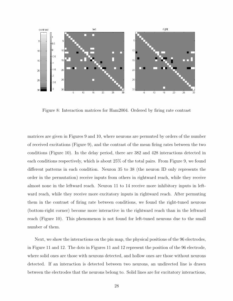
Figure 8: Interaction matrices for Ham2004. Ordered by firing rate contrast
matrices are given in Figures 9 and 10, where neurons are permuted by orders of the number
of received excitations (Figure 9), and the contrast of the mean firing rates between the two
conditions (Figure 10). In the delay period, there are 382 and 428 interactions detected in
each conditions respectively, which is about 25% of the total pairs. From Figure 9, we found
different patterns in each condition. Neuron 35 to 38 (the neuron ID only represents the
order in the permutation) receive inputs from others in rightward reach, while they receive
almost none in the leftward reach. Neuron 11 to 14 receive more inhibitory inputs in left-
ward reach, while they receive more excitatory inputs in rightward reach. After permuting
them in the contrast of firing rate between conditions, we found the right-tuned neurons
(bottom-right corner) become more interactive in the rightward reach than in the leftward
reach (Figure 10). This phenomenon is not found for left-tuned neurons due to the small
number of them.
Next, we show the interactions on the pin map, the physical positions of the 96 electrodes,
in Figure 11 and 12. The dots in Figures 11 and 12 represent the position of the 96 electrode,
where solid ones are those with neurons detected, and hollow ones are those without neurons
detected. If an interaction is detected between two neurons, an undirected line is drawn
between the electrodes that the neurons belong to. Solid lines are for excitatory interactions,
28

Figure 9: Interaction matrices for Larry2008 in the delay period. Ordered by numbers of
received excitations
Figure 10: Interaction matrices for Larry2008 in the delay period. Ordered by firing rate
contrast
29

and dash lines are for inhibitory interactions. We found that the recorded neurons are
concentrated in the left and bottom. The four neurons in the upper right introduce more
inhibitions in the rightward reach. To highlight this, we only show inhibitory interactions in
the pin map in Figure 12.
Figure 11: Interactions on the pin map for Larry2008 in the delay period.
Further, we analyze neuronal interactions in the pre-cue period to compare the network in
the delay period. To make a better comparison, the interaction matrices in Figure 13 and 14
are shown with neurons in the same orders as in Figure 9 and 10 respectively. From Figure
13, we can see a great difference in the both the amount and the pattern of interactions
between the two conditions. There are only 80 detected interactions (5%) in the leftward
reach and 168 (10%) in the rightward reach. Neurons 5 to 15 in Figure 13 receive inputs
from other neurons in the rightward reach, while they hardly receive any in the leftward
reach. The neurons which are tuned either leftward or rightward now show no interactions
with each other (Figure 14).
Interactions are also plotted in the pin map (Figure 15). Inhibition does not occur in the
upper-right four neurons as in the delay period. Compared to the delay period, inhibitions
do not occur often in pre-cue period at all.
30

Figure 12: Inhibitory interactions on the pin map for Larry2008 in the delay period.
Figure 13: Interaction matrices for Larry2008 in the pre-cue period. Neurons are in as the
same order as in Figure 9
31

Figure 14: Interaction matrices for Larry2008 in the pre-cue period. Neurons are in as the
same order as in Figure 10
Figure 15: Interactions on the pin map for Larry2008 in the pre-cue period.
32

3.6 DISCUSSION
In sum, the results from Ham2004 and Larry2008 show interesting features of the interac-
tions between neurons. Although these results are not strong enough to make any solid
physiological conclusions yet, the proposed method offer a tool to identify a sparse network
of short-term interacting neurons from the entire ensemble activity, going well beyond the
more classical study of pairwise interactions. The detected network, or particular interac-
tions between neurons of interest, can be highlighted by the model from raw data for further
examination. We have justified, to some extent, the adequacy of the L1-regularized logis-
tic model using both theoretical and simulation studies. Although computation for such
problems is quite heavy in general, our approach has several features that make computa-
tion feasible. First, we use regularization to avoid certain nonconvergence problems that a
naive implementation of GLM would encounter [65]. Second, we use the coordinate descent
algorithm, which is efficient and easily implemented. Third, we use the BIC γ-selector to
determine the tuning parameter. We recognize that cross-validation is common, but it is
much more computationally intensive because it requires repeated model fitting; in addition,
we provide a theoretical justification for the use of the BIC γ-selector. And fourth, we de-
compose the regression model into C individual sub-models, each with considerably smaller
dimensionality. This decomposition is especially effective when the number of neurons is
large, which is important as advances in technology allow for the simultaneous recording of
increasing numbers of neurons.
With current information about the experiments, we cannot well explain some inconsis-
tency between the results of two different monkeys. However, we note that the experiments
on Ham and Larry were made in different years. Also, the experimental parameters are
not totally consistent, not to mention the possible uncontrolled even unknown effects, like
fatigue, neuronal adaptation or circuit from outside the recorded area. We will continue the
collaboration with colleagues in neuroscience, and seek data where the proposed method can
shed more light on the physiology.
33

4.0 A VARIABLE COEFFICIENTS MODEL FOR THE VARIATION OF
NEURONAL INTERACTIONS ACROSS TRIALS
4.1 VARIABLE COEFFICIENTS MODELS
In equation (2.2), the parameters are treated as constant with respect to both t and j. It
is probably true for βcp, because they represent the refractoriness, an intrinsic property of
neurons. However, the baseline firing rate parameter βc and interaction parameters βicq can
change within a trial or across trials. Here we focus on the across-trial variation of baseline
firing rates and neuronal interactions, and treat the corresponding parameters as functions
of j: βc(j) and βicq(j), j = 1, . . . , J . Thus, the generalized linear model (2.2) turns a variable
coefficient model [29].
For a better illustration of this approach, we reparametrize the model (2.2) with variable
coefficients into a general form. Assume there are T bins within each trial and J trials in
total. Assume the responses ytj, the count of spikes in bin t at trial j, has a Bernoulli or
Poisson distribution ftj(y) with mean µtj. Then we build a generalized linear model with
variable coefficients:
g(µtj) = θ0(j) +N∑i=1
θi(j)utij +M∑i=1
βivtij, (4.1)
where t = 1, . . . , T , j = 1, . . . , J .
In (4.1), θ0(j) is the variable intercept, and θi(j), i = 1, . . . , N represent N variable
coefficients for the interactions. Further, assume that all the variable coefficients θi(j),
34

i = 0, . . . , N , are can be represented as linear combinations of a preassigned set of basis
functions Φ1(j), . . . ,ΦB(j):
θi(j) =B∑b=1
φibΦb(j).
The parameters βi, i = 1, . . . ,M , in the third term of (4.1), are constant, representing effects
other than neuronal interactions. Finally, the g(·) is the appropriate link function for either
logistic or Poisson models, depending on whether the responses are binary or count data.
Denote the response vector Y = (y11, . . . , yT1, . . . , y1J , . . . , yTJ)′, and the parameter vec-
tor Θ = (φ01, . . . , φ0B, . . . , φN1, . . . , φNB, β1, . . . , βM)′. Further, denote Ψj = (Φ1(j), . . . ,ΦB(j))
and
Uj =
1 u11j . . . u1Nj
......
......
1 uT1j . . . uTNj
, and Vj =
v11j . . . v1Mj
......
...
vT1j . . . vTMj
Thus, the design matrix X has the form:
X =
U1 ⊗Ψ1 V1
......
UJ ⊗ΨJ VJ
,
where ‘⊗’ is the Kronecker product. With the response vector Y , the design matrix X,
the parameter vector Θ and distribution functions {ftj(·)}, we can explicitly write the log-
likelihood l(Θ|X, Y ); see [34] for details. In this augmented GLM problem, the sample size
is n = T × J and the number of parameters is p = B × (N + 1) +M .
Instead of maximizing the log-likelihood l(Θ|X, Y ), we optimize a doubly penalized ver-
sion of it. The first one is the smoothing penalty on the squared second derivatives of
{θi(j)}i, and the other one is the mild L2 penalty on {βi}i to avoid an infinite maximum
[65]. Therefore, we actually minimize:
−2l(Θ|X, Y ) +N∑i=0
λi
∫θ2i (j)dj + γ
M∑i=1
|β2i | (4.2)
Denoting S =∫
Ψ′(j)Ψ(j)dj and I the identity matrix, expression (4.2) can be further
reduced to
−2l(Θ|X, Y ) + Θ′HΘ, with H = diag(λ0S, . . . , λNS, γI). (4.3)
35

The minimization of (4.3) and the inferences can be done by IRLS algorithm [34, 62]. Here
I brief sketch this algorithm:
1. With an initial value Θ(0), compute the pseudo-values Z(0) and weight matrix W(0).
2. Denote Z∗(k) =√W(k)Z(k) and X∗(k) =
√W(k)X(k). Update Θ by letting Θ(k+1) =
(X∗′
(k)X∗(k) +H)−1X∗
′
(k)Z∗(k).
3. Use the new Θ(k+1) to compute the Z(k+1) and W(k+1).
4. Repeat step 2-3 until convergence.
We have the converged {Θ(k)} and use the last iteration as the estimation of parameters,
from which the variance of estimated parameters, degrees of freedom and sum of squared
residuals can be easily computed:
Θ = limk
Θ(k),
V (Θ) = limk
(X∗′
(k)X∗(k) +H)−1X∗
′
(k)X∗(k)(X
∗′(k)X
∗(k) +H)−1,
df = limktr(X∗(k)(X
∗′(k)X
∗(k) +H)−1X∗
′
(k)),
SSR = limk‖ Z∗(k) −X∗(k)Θ ‖2 .
4.2 GCV, CONFIDENCE BANDS AND HYPOTHESIS TESTING
Since the second penalty in (4.2) is only for avoiding an infinite maximum, γ can be preas-
signed to a small value, say 0.1, such that (X∗′
(k)X∗(k) + H) is invertible. On the other hand,
the tuning parameters λ = (λ0, . . . , λN) should be selected by data, because we do not know
the actual degrees of smoothness. According to Wood (2006) [62], the optimal λ can be
chosen by minimizing the generalized cross validation score:
GCV (λ) =n× SSR(n− df)2
For small dimension of λ, say one or two, the optimization of GCV (·) can be done by a
grid search in λ space. However, it will become less efficient, even infeasible, when the
dimension of λ is large, which is the usual case when dealing with spike train data. Wood
36

[61, 63] suggested the Newton-Raphson algorithm to optimize the GCV (·). For doing so,
he analytically evaluated the exact gradient and Hessian in Wood (2008) [63]. However, the
calculation of the exact gradient and Hessian involves heavy computation, and it is hard
to implement. An earlier method proposed by Wood (2004) [61] would be considered more
efficient by the author, where the inexact gradient and Hessian are calculated by treating the
weight function W and pseudo-values Z as invariants to λ in each IRLS iteration. But Wood
(2004) [61] suggested a QR-decomposition of the design matrix X. This decomposition will
become computationally intensive, even infeasible, when the sample size n is extremely large.
Suppose n = 100, 000, which can happen in a real spike train data, thus the Q matrix will be
100, 000×100, 000 in dimension. In addition to the time required for a QR-decomposition of
a 100, 000× p matrix, the storage of the matrix Q will first become a serious issue. Assume
the Q stored in a double precision, which takes 8 bytes of memory per variable. The total
memory required by Q would be 80GB!
To avoid this problem, all matrices in the calculation should be confined to a manageable
size, and at most matrix multiplication, trace operation and inversion should be involved.
For example, avoid operations on n × n matrices, or store the diagonal weight matrix W
in vector form rather than a matrix. By doing this, the Newton-Raphson algorithm will be
feasible on an ordinary PC. The computer will calculate the inexact gradient and Hessian
in each IRLS iteration in a reasonable time. Please see Appendix B for the details of the
expressions of those derivatives.
Because the L2 penalty term in (4.3) can be treated as an improper Gaussian prior
(H may not have full rank) of the parameters from a Bayesian perspective, the point-wise
confidence bands for variable coefficients {θi(j)}i can be constructed by finding their posterior
mean and covariance matrix [51]. In the variable coefficients model (4.3), the posterior mean
is Θ and covariance matrix is Vpost = (X∗′
(k)X∗(k) + H)−1 [51, 62]. However, the posterior
mean and covariance matrix of the parameters are conditional on the selected smoothing
parameters λ. Since λ are selected by data, bias can be introduced. Therefore, we construct
unconditional Bayesian confidence bands introduced by Wood [62], where we first bootstrap
samples of λ so that we collect a pool of posterior means and covariance matrices under
different λ. Based on the unconditional means and covariance matrices, we further construct
37

95% simultaneous confidence bands for θi(.) via the method introduced by Ruppert, Wand
and Carroll (2003) [47]. Since both methods are based on a parametric bootstrap [62, 47], to
construct the 95% simultaneously unconditional Bayesian confidence bands, we unified the
two algorithms so that the bootstrap samples can be efficiently used. Here is the outline of
the unified algorithm:
1. Get Θ by fitting model (4.3) and minimizing the GCV score.
2. Loop from k = 1 to Nu
• Generate a response vector Y (k) from design matrix X, parameters Θ and the cor-
responding distribution in some exponential family (Bernoulli or Poisson).
• With Y (k) and X, get Θ(k) and V(k)post by fitting model (4.3) and minimizing the GCV
score.
• store Θ(k) and V(k)post for later usage.
3. loop from l = 1 to Ns
• Randomly sample a number k from {1, 2, . . . , Nu}.
• Generate Θ(l) from N(Θ(k), V(k)post).
• Let θ(l)i (·) =
∑Bb=1 φ
(l)ib Φb(·), andm
(l)i = maxj{ |θ
(l)i (j)−θ(l)i (j)|σ(θ
(l)i (j))
}, where θ(l)i (j) =
∑b φ
(k)ib Φb(j),
i = 0, . . . , N , and σ(θ(l)i (j)) can be computed from Ψj and V (k).
• store θ(l)i (·) and m
(l)i , i = 0, . . . , N .
4. Denote mi as the 95% quantile of {m(1)i , . . . ,m
(Ns)i }. The lower (upper) bound Li(·)
(Ui(·)) for θi(·) is the mean of {θ(l)i (·)}l minus (plus) mi times the standard deviation of
{θ(l)i (·)}l.
In practice, I choose Nu = 20 and Ns = 10, 000, as suggested by Wood [62] and Ruppert et
al. [47].
Although the simultaneous confidence bands give a range of the variable coefficients, it
is not valid to infer that the true curve is of a certain form just because the curve with that
form falls in the confidence bands [47]. Therefore, we need a hypothesis testing procedure
to infer the simpler structure of the the variable coefficients; for example, we test whether
the coefficient θi(j) is a constant in j. Under the penalized spline in GLM framework,
we use the likelihood ratio test introduced by Wood [62], assuming that the test statistic
38

has a χ2 null distribution [28, 29, 62]. Letting subscript F stand for the full model and
subscript R for the reduced model, the likelihood ratio for the two candidate models is
LR = 2(l(ΘF |XF , Y ) − l(ΘR|XR, Y )). This test statistic LR approximately has the χ2
distribution with the degrees of freedom dfF − dfR [62].
4.3 SIMULATION STUDY
4.3.1 Single-input network
We did simulation studies to assess the adequacy of the proposed model. First we simulated
a neuron with one excitatory input; see Figure 16. Neuron Two was excited by Neuron
Figure 16: The simulated single-input network and the parameter setup
One, and their spiking activities function according to model (3.1). The baseline firing rates
39

of both neurons are set to 25Hz at the beginning, while the baseline firing rate of Neuron
Two will decrease from 25Hz to 10Hz across trials, by letting β2 decrease exponentially. The
excitatory interaction from Neuron One will also decrease across trials by letting β211 decrease
exponentially from 4 to 2. The self-history effect parameters βcp are set constant across trials.
In this simulation, the recording period in one trial is 500 ms, and 100 trials are generated.
Using the simulated data, the coefficient curves are fitted by the variable coefficients model.
The confidence bands are also constructed. The results are shown in Figure 17. Solid lines
are the actual coefficient curves, dash lines in the middle are the fitted curves, and the dash
lines folding the fitted curves are 95% simultaneously confidence bands. We can see that the
Figure 17: The fitted curves of the baseline firing rate (left) and the excitatory interaction
(right) with confidence bands
fitted coefficient curves well capture the exponentially decreasing trend, and the confidence
bands suggest that the interaction from Neuron One is significantly positive all the time.
Further, we use the likelihood ratio test to verify the variation of the baseline of Neuron
Two and the excitatory interaction from Neuron One to Neuron Two across trials. We fit a
reduced model with a constant β211(j) for all j, and a reduced model with a constant β2(j)
for all j. The test statistics are respectively LR = 7560.7 − 7513.8 = 46.9 with degrees
of freedom 72.673 − 66.571 ≈ 6 and LR = 7563.0 − 7513.8 = 49.2 with degrees of freedom
72.673−67.9562 ≈ 5. The corresponding p-value for testing the variable baseline is < 0.0001,
and < 0.0001 for testing the variable interaction. Thus, the variation of the baseline and
interaction are both significant across trials.
40

4.3.2 Multiple-input network
Next, we simulate a network where a neuron receives multiple inputs: see Figure 18, where
Neuron One interacts with six neurons. In the cortex, one neuron can interact with more
than 6 other neurons, but the results of interaction detection in previous chapter suggest a
lower dimensional problem. In the simulated network, Neuron Two, Three and Four excite
Neuron One, and Neuron Five, Six and Seven inhibit it. We also include a Neuron Eight
that has no interaction with Neuron One. The baseline firing rates of all eight neurons
are set to 25Hz and invariable across trials. The three excitatory interactions are set as 1)
exponentially decrease from 4 to 2; 2) exponentially increase from 2 to 4; 3) quadratic change
from 4 to 4 with a minimum at 2. Similarly, the three inhibitory interactions are set as 1)
exponentially decrease from -4 to -2; 2) exponentially increase from -2 to -4; 3) quadratic
change from -4 to -4 with a minimum at -2. See Figure 18 for details. Just as in the previous
simulation, the recording period in one trial is set to 500 ms, and the trials are repeated by
100 times.
Figure 18: The neuron with multiple inputs and the parameter setup
The coefficient curves are fitted by the variable coefficients model, and the confidence
bands are constructed. The results are shown in Figures 19, 20 and 21. Again, solid lines
stand for the actual curves, and dashed lines are for the fitted curves and confidence bands.
For excitatory interactions, the fitted coefficient curves well capture the variation and con-
41

fidence bands suggest that the excitatory interactions are significantly positive all the time
(Figure 19). The fitted curves capture the variation in inhibition well too. However, the
confidence bands for inhibitory interactions are extremely wide, so that it is hard to infer
that the inhibitions are significant (Figure 20). For the constant baseline of Neuron One,
confidence bands suggest the range of baseline firing rate for Neuron One. The fitted curve,
although not completely flat, varies between -3.7 to -3.5 (Figure 21A). In the end, Neuron
Eight is supposed to be independent of Neuron One, and confidence bands show no signif-
icance in the existence of interaction between them. However, the fitted curve showed a
sinusoidal variation across the trials (Figure 21B). That could be just due to the error, and
we will use the likelihood ratio test to further study it.
Figure 19: The results for the three excitatory interactions
Figure 20: The results for the three inhibitory interactions
To further infer the variation of the interactions and the baseline firing rate across trials,
we do five groups of likelihood ratio tests to test: 1) the variation of the three excitatory
interactions, 2) the variation of the three inhibitory interactions, 3) the existence of the three
42

Figure 21: The results for A) the baseline, and B) the independence to Neuron Eight
inhibitory interactions, 4) the variation of the baseline firing rate, and 5) the existence of the
interaction from Neuron Eight. See Table 6 for details. The p-values in Line One of Table 6
Table 6: The hypothesis testing results for the baseline and interactions
Test # test statistic degrees of freedom p-value
1) 77.31, 71.26, 93.75 5, 5, 5 < 0.0001, < 0.0001, < 0.0001
2) 10.94, 5.58, 19.62 2, 2, 2 0.0042, 0.061, < 0.0001
3) 320.61, 277.73, 278.68 3, 3, 3 < 0.0001, < 0.0001, < 0.0001
4) 7.57 6 0.27
5) 9.99 5 0.075
show that the three excitatory interactions are significantly variable across trials. The three
types of inhibitory interactions are also significantly variable, although this conclusion might
be less solid than that from excitations. Note p-value 0.061 in Line Two for the inhibition
from Neuron Six. Putting aside the argument about the variation in the three inhibitory
interactions, they at least significantly exist (non-zero) during all trials due to the p-values
in Line Three. The p-values 0.27 in Line Four and 0.075 in Line Five suggest a constant
baseline firing rate and no interaction from Neuron Eight, which comply with the simulated
43

network.
In sum, the two simulation studies indicate the good performance of the variable coeffi-
cients model and the accompanying inference methods for the variation of the interactions
across trials. The fitted curves well capture some basic features of the variation, such as
monotone, quadratic or constant trends. Consistent with the results in interaction detec-
tion, the model works better for excitatory interactions than for inhibitory interactions.
Again, we speculate that it is because the baseline is so low that inhibition is not as obvi-
ous as excitations. Nevertheless, the likelihood ratio test can at least infer the significant
presence of inhibitory interactions. Comparing the confidence bands inference to likelihood
ratio tests, the former is more conservative. Therefore, in real data analysis, we will base
inferences primarily on the likelihood ratio test, with confidence bands as secondary.
4.4 MONKEY DATA RESULTS
Next we will apply the variable coefficients model to real monkey data. Section 2.1 has the
details of the experiments and data; Equation (3.1) and Section 4.1 detail the model and
parameters setup; and Section 3.5 gives the results of interaction detection, upon which the
following analysis is based.
First, we will use the variable coefficient model to examine single-input networks. In the
detected network of Larry2008, we noticed Neuron 38 is only inhibited by Neuron 13 over all
trials (Figure 22). Therefore, we study whether this inhibitory interaction is variable across
trials. The fitted curves and confidence bands are shown in Figure 22. We found that the
intercept β38 fluctuates between -5 to -4.5, which corresponds to the baseline firing rates
of Neuron 38 fluctuating from 6.7Hz to 11Hz. No obvious increase or decrease is found in
the baseline firing rate of Neuron 38. The likelihood ratio test indicates significant variation
(LR = 13591.21− 13554.14, df = 80.08− 67.21 and p-value = 0.0004). On the other hand,
the inhibitory interaction from Neuron 13 to Neuron 38 is quite insignificant across trials
due to the wide band of the confidence bands. From the fitted curve, we do not see a clear
trend. Therefore, we resort to likelihood ratio test. We further fit two reduced models, one
44

with constant interaction, and the other without interaction. Together with the full model,
the three −2 logL are 13554.14 (full model), 13561.97 (constant interaction) and 13594.84
(no interaction). The degrees of the freedom for the three models are 80.08 (full model),
72.17 (constant interaction) and 71.17 (no interaction). The p-value for testing the variable
interaction is 0.4499, so there is no significant variation across trials in this interaction. The
p-value for testing the existence of the interaction is < 0.0001, so the inhibitory interaction
is significant.
Figure 22: Larry2008, Neuron 38. The network (up) and fitted curves with confidence bands
(bottom)
Another single-input network we chose for analysis is from Ham2004, a detected excita-
45

tory interaction from Neuron 9 to Neuron 14 (Figure 23). The fitted curves and confidence
bands are shown in Figure 23. We found the baseline firing rate of Neuron 14 fluctuates
around -4.5, which correspond to 11Hz. But there is a decrease in the first 30 trials. The
likelihood ratio test also suggests significant variation across trials (p-value< 0.0001). As for
the interaction, the confidence bands are so wide that the excitatory interaction from Neuron
9 may not be significant. Thus, we further use two likelihood ratio tests to examine whether
the interaction is variable across trial and whether it significantly exist at all. The −2 logL
for the full model, constant interaction model and no interaction model are 8619.3, 8626.1
and 8629.7 respectively. The degrees of freedoms are 74, 70 and 69. The p-value for testing
the variable interaction model is 0.14, and 0.07 for testing the existence of the interaction.
This suggests that the excitatory interaction from Neuron 9 to Neuron 14 is weak.
Next, we examine the neurons with multiple inputs. We choose Neuron 9 in Ham2004
data. From the preliminary detection of interactions, Neuron 9 receives five excitatory
inputs from Neuron 3, 14, 16, 24 and 28, and one inhibitory input from Neuron 8 (Figure
24). Applying the variable coefficient model to this seven-neuron network, we get the curves
of the baseline of Neuron 9 and six interactions across trials (Figure 25). From the Figure
25, we find there is variation in the baseline firing rate of Neuron 9. It decreases during the
first 25 trials, then increases to a higher level, and maintains at that level during the last
50 trials. As for those interactions, the confidence bands are so wide that we can barely
infer any variation from it. However, noting the much wider confidence bands at first fifty
trials in all five excitatory interaction curves, we suspect instability in the first fifty trials.
To highlight that, we draw all fitted curves in the same coordinate without confidence bands
(Figure 26). From Figure 26, we can see all five excitatory interactions become stable after
the first fifty trials. They either increase or decrease during the first 50 trials. Three of
them even begin with inhibition. The only inhibitory interaction from Neuron 8 to Neuron
9 also shows variation. It is excitatory for the first fifty trials, but gradually decreases to an
inhibitory interaction in the next fifty trials. In the last fifty trials, the strength of inhibition
was rapidly enhanced. Therefore, we can see the neuronal activity vary across trials roughly
in three stages.
We also put the curves from Neuron 14 in our previous analysis with those of Neuron 9
46
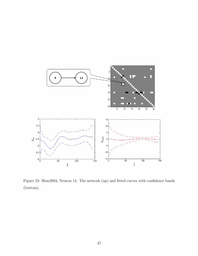
Figure 23: Ham2004, Neuron 14. The network (up) and fitted curves with confidence bands
(bottom).
47

Figure 24: Ham2004, Neuron 9. The network.
(Figure 27). We can again see the baseline of Neuron 14 and the interaction from Neuron 9
to Neuron 14 also vary roughly in three stages.
We use likelihood ratio tests to further validate our findings about variation. See Table 7
for the results. From those p-values, we did not find much variation among the five excitatory
interactions. Even the existence of some of them (Neuron 3, Neuron 24) is not significant.
We suspect this phenomenon, together with the wide confidence bands, is due to the unstable
dynamics in the first fifty trials. Nevertheless, the variable coefficient model does successfully
elucidate the variation in interactions across trials, which is important for us in our search
for the physiological message it brings.
4.5 DISCUSSION
According to the simulation study, the variable coefficients model can effectively capture the
variation of interactions across trials. Monkey data Ham2004 also suggest a roughly three-
stage change of physiology across the one-day session, which arise our interest in exploring
48

Figure 25: Ham2004, Neuron 9. The fitted curves with confidence bands.
49

Figure 26: Ham2004, Neuron 9. All fitted curves in one coordinate.
50

Figure 27: Ham2004, Neuron 9 and Neuron 14. All fitted curves in one coordinate.
51

more on this issue. In the future, we plan to study different monkey data from Dr. Batista’s
lab, where two sessions — an early session during a certain experiment and then a later
session when we expect that the monkey has gotten used to the experiment. We hope to
find variations of interactions due to the this change in the monkey’s performance during
the experiment.
As for the methodology, among various works in this context, we are particularly inter-
ested in interpreting penalized splines into a generalized linear mixed-effect model (GLMM)
framework. If the L2 penalty term in (4.3) is treated as mixed effects, equation (4.3) is equiv-
alent to the likelihood of a GLMM [47]. In the GLMM framework, the smoothing parameters
λ are related to the variances of the random effects, so they can be conveniently estimated
by restricted maximum likelihood (REML) [47]. This offers a new way to select smoothing
parameters. Compared to prediction-error-based methods such as GCV, the maximum-
likelihood-based methods such as REML tend to give much smoother estimates (Ruppert
et al. 2003, pp.122). In addition, under the GLMM framework, research about confidence
intervals and hypothesis tests has been widely done too. Krivobokova et al. (2010) [31]
offer a new way to construct simultaneous confidence bands instead of via Bayesian meth-
ods. A series of works by Crainiceanu and his colleagues focus on the exact likelihood ratio
tests with certain polynomial functions as null hypotheses [13, 14]. Although that work of
Crainiceanu and his colleagues is mainly based on polynomial basis spline, the idea is worth
pursuing in the future. For example, because the null distribution of the likelihood ratio
test we used in the previous sections is not theoretically justified, we can rely on parametric
bootstrap instead to get its sampling distribution, as suggested in Crainiceanu and Ruppert
(2004) [13].
52

Table 7: The hypothesis testing results for the baseline and interactions of Neuron 9
Test test statistic degrees of freedom p-value
H0: β9 = c 595.86 9 < 0.0001
H0: β9,3,1 = c 3.00 5 0.7
H0: β9,3,1 = 0 6.15 6 0.4
H0: β9,8,1 = c 12.75 4 0.012
H0: β9,14,1 = c 8.97 4 0.06
H0: β9,14,1 = 0 8.97 5 0.007
H0: β9,16,1 = c 9.4 5 0.094
H0: β9,16,1 = 0 13.86 6 0.03
H0: β9,24,1 = c 3.7 4 0.45
H0: β9,24,1 = 0 10.57 5 0.06
H0: β9,28,1 = c 11.73 5 0.039
H0: β9,28,1 = 0 18.88 6 0.0044
53

5.0 NONCONVERGENCE IN LOGISTIC AND POISSON MODELS FOR
NEURONAL SPIKING
5.1 THE NONCONVERGENCE PROBLEM
The GLM framework, of which the logistic and Poisson models are most popular, is now
well established in quantitative studies in neuroscience [6, 37, 55]. In particular, the log-
likelihoods that arise in GLMs are typically concave. Thus, maximum likelihood estimates
(MLEs) and their corresponding confidence intervals are usually efficiently computed using
iterations of least squares calculations, which are well understood [34]. Typical criteria
for stopping the iterations require sufficiently small (relative or absolute) changes in the
parameter values, in the log-likelihood values, or a combination of the two [3].
These algorithms, however, are not foolproof. They are susceptible to either nonconver-
gence or false convergence (criterion met, but the final value is far from optimal). In general,
these difficulties can arise for several reasons: the log-likelihood may be multimodal, the
covariates may be close to collinear, or the sample size may not be large enough compared
to the number of parameters. Throughout this chapter, we assume that the sample size is
larger than the number of parameters to be estimated. We argue below that for logistic
and Poisson regression these difficulties arise, instead, because the log-likelihood achieves
its maximum at an infinite value of a regression coefficient. For the logistic model, these
data configurations are known as complete separation (CS) and quasi-complete separation
(QCS) [2, 50, 49]. For the Poisson model, we characterize the configurations under which
the maximum likelihood estimate (MLE) is not finite. For both models, we show how to use
linear programming methods to detect these configurations.
There are theoretical studies that give rather general conditions for the existence and
54

uniqueness of MLEs for exponential families, which underlie GLMs [4]; however, they do
not deal with the specifics encountered in this context. Our aim here is to provide a formal
treatment of this topic and to provide criteria for detecting difficulties that are readily
implemented. We start with the logistic model, for which we define CS and QCS, and
describe their geometry. We describe the relationship between a neuron’s refractory period
and convergence difficulties due to binning conventions. We then show how commonly used
software (MATLAB, SAS) deals with such difficulties. We turn to analogous matters for
the Poisson model. We also state and prove conditions under which regression parameter
estimates are infinite, and provide a numerical example which models bursting activity. We
conclude with a discussion of the merits of several possible remedies. We put technical details
such as formal proofs and the linear programming formulation in the Appendix.
5.2 INFINITE MLE IN LOGISTIC REGRESSION
We start with the logistic model for spike train data analysis. The logistic regression models
for spike train data were introduced in section 2.2; see equation (2.2). For our purposes, a
generic form of this model suffices. For a binary outcome Y with values 0 or 1, intercept
term and covariates x = (x1, . . . , xs)′, and parameter vector β = (β1, . . . , βs)
′, the logistic
model for P (Y = 1|x) = p(x) is
logit[p(x)] =s∑i=1
βixi = β′x (5.1)
Henceforth, we assume that x1 ≡ 1, so that β1 is the intercept.
5.2.1 Complete and quasi-complete separation
Silvapulle (1981) and Albert and Anderson (1984) studied the problem of determining when
the MLEs of the regression parameters are finite [2, 50]. In short, the MLEs are finite if and
only if neither CS nor QCS holds. Albert and Anderson’s geometric interpretation of these
configurations is easy to state. First define x− = (x2, . . . , xs)′. Then, CS means that there is
55

perfect prediction through a linear combination: that is, there is some vector a and a scalar
b such that a′x− > b (a′x− < b) corresponds to Y = 1 (Y = 0), so that the two outcomes
are separated by a plane. QCS allows for overlap at the boundary of the two regions: thus,
a′x− ≥ b (a′x− ≤ b) corresponds to Y = 1 (Y = 0). Figure 28 depicts these two cases, along
with the other possible configuration, overlap, for which no plane in the covariate space
separates the two outcomes.
Figure 28: The configurations
The relevance of CS and QCS to the analysis of spike trains is given in the following
proposition, whose proof is in the Appendix C.
Proposition: If the refractory periods prevent spikes in consecutive bins, then CS or QCS
will occur.
In particular, this proposition applies to the choice of 1 ms bin size. This proposition is
quite general: it depends only on the refractory period, and not on other aspects of the
model. When the number of covariates is at most three, an inspection of plots of the data
is enough to decide which of CS, QCS, or overlap holds. However, when C, the number
of neurons involved is large, the dimensionality is high enough to make graphical methods
infeasible, and the determination of a and b difficult. For such cases, analytic approaches are
necessary. Silvapulle gave a characterization of the configuration of covariates that yield a
finite MLE: see the Appendix C. A linear programming characterization of these conditions
is the following: first partition the design matrix thus: X = (X0, X1)′, where the superscript
56

corresponds to the value of the response. Then consider the linear inequality array in the
variable a: X0
−X1
a ≤ 0
If there are nontrivial (nonzero) solutions to this inequality, then QCS or CS obtains. For
details of how to use linear programming procedures to determine the existence of nontrivial
solutions for linear inequalities see the Appendix E.
5.2.2 An example
Suppose that in the logistic model (5.1) we ignore network and stimulus effects, and focus
only on the neuron’s spiking history. Suppose further that for a particular bin size, the
refractory period prevents spikes in two consecutive bins. The spike train then plays the role
of both the covariate and outcome. Let x indicate the presence of a spike in a particular bin
and y indicate the presence of a spike in the next bin. Then, the following data are possible:
x: 0 0 0 0 0 0 0 0 1 1 1 1
y: 1 1 1 1 0 0 0 0 0 0 0 0
Note that as the likelihood function does not depend upon the order of the (x, y) pairs.
We have sorted the data in this example according to the y values; this sorting makes it
clear that QCS holds, with the sets x ≤ 0 and x ≥ 0 quasi-separating the two outcomes.
The MATLAB code and output using the glmfit command are:
MATLAB Code:
>> y=[1,1,1,1,0,0,0,0,0,0,0,0]’;
>> x=[0,0,0,0,0,0,0,0,1,1,1,1]’;
>> b=glmfit(x,y,’binomial’,’link’,’logit’)
MATLAB Output:
Warning: Iteration limit reached.
> In glmfit at 355
b = -0.0000, -102.5661
Given QCS data, MATLAB appropriately gave a warning that the iteration limit was
reached; its estimate of the slope coefficient, −102.57, is large. While this warning is a good
57

feature of MATLAB, it is of limited use because it does not identify QCS as the cause of the
lack of convergence. Other software packages are uneven on this matter. For example, con-
sider the LOGISTIC and GENMOD procedures in SAS. The LOGISTIC procedure correctly
stated that ‘Quasi-complete separation of data points detected’; thus, it checks for QCS and
provides a warning when needed. However, the GENMOD procedure — which monitors both
changes in parameter estimates and a function of the log-likelihood, and it terminates when
either criterion is met — converged falsely and gave test statistics for assessing goodness of
fit. Albert and Anderson have shown that the log-likelihood is always bounded above; thus,
iterations for maximizing the log-likelihood asymptote towards that bound when either CS
or QCS hold. This example shows that the use of a second convergence criterion can still
lead to false convergence. It is likely that MATLAB uses changes in the successive parameter
estimates: in this case, the MLE of β1 is at infinity, to which the estimates are tending.
5.3 THE POISSON MODEL
A common fix for nonconvergence in the logistic model is to enlarge the bin size so that a bin
allows more than one spike per bin. In that case, Poisson regression is an appropriate model.
Here we show that nonconvergence can occur for the Poisson model too. We again work with
a generic form of the model: reordering the data, we have n independent count responses yi
for i = 1, ..., n, with yi = 0 for i = 1, ..., r and yi > 0, for i = r+ 1, ..., n. Suppose that yi has
a Poisson distribution with mean µi, and that the corresponding s-dimensional covariates
and intercept are given in the vector xi. Writing ηi = x′iβ, the relationship between response
and covariates is given by the link function
g(µi) = x′iβ = ηi
The standard Poisson link between the mean and covariates is g(t) = log(t). However,
other functions arise in specific circumstances: for example, Paninski [37] considers g that is
logarithmic in one region and linear in another. For technical reasons, here we assume that
g is an increasing twice-differentiable function with the entire real line as its range. Let li(β)
58

be the log-likelihood for the ith pair (xi, yi). Then the log-likelihood function for the entire
data set is (up to an additive constant)
l(β) =n∑i=1
li(β) =n∑i=1
[yi log µi − µi] =n∑
i=r+1
[yi log µi − µi]−r∑i=1
µi
=n∑
i=r+1
[yi log g−1(xiβ)− g−1(xiβ)]−r∑i=1
g−1(xiβ) = S1 − S2 (5.2)
To fully characterize the existence of the MLE for the Poisson model, we need certain
algebraic preliminaries for the n× s design matrix X = (x′1, . . . , x′n)′. First, assume that X
has full rank, that is, rank(X) = s; next, let X0 = (x′1, . . . , x′r)′ denote the r × s part of the
design matrix corresponding to the zero spike counts (recall that yi = 0 for i = 1, . . . , r);
and let X+ = (x′r+1, . . . , x′n)′ denote the (n − r) × s matrix corresponding to positive spike
counts. Suppose that rank(X+) = s− q with q = 0, 1, . . . , s. If X+ is not of full rank, then
there is an s × q matrix Γ, with rank q such that X+Γ = (0, ..., 0)′. Finally, call a vector
a in Rs ‘negative’ and write a < 0 if each component of a is nonpositive and at least one
component is negative; otherwise call a ‘nonnegative’, and write a ≮ 0.
Given the log-likelihood in (5.2) and the algebraic preliminaries, we now sketch an in-
tuitive argument that leads to a characterization of the existence of a finite MLE for Pois-
son regression. First, for any data configuration, the maximum must have finite values
for ηi, i = r + 1, . . . , n because positive counts preclude zero estimates of µi; hence, S1 in
(5.2) is well behaved. Note that if X+ does not have full rank, solutions of the equation
X+β = (ηr+1, . . . , ηn)′ can allow infinite β’s. Next, for the∑r
i=1 g−1(xiβ) component there,
the infinite components in β can cause either g−1(−∞) = 0, which maximizes the log-
likelihood, so the maximum is at infinity; or g−1(∞) = ∞, which makes the log-likelihood
equal to −∞, so a maximum at infinity is precluded. Hence, the criterion must involve
X0. Next, in order to guarantee that S1 is unchanged when we examine the influence of
the infinite β components on S2, we note that X0Γ corresponds to the part orthogonal to
the subspace spanned by X+. We now state the necessary and sufficient condition for the
existence of a finite MLE; the proof is in the Appendix D.
59

Theorem. For the Poisson regression model given in (5.2) with a link function g as de-
scribed above, the MLE is finite if and only if X0Γa ≮ 0 for any a ∈ <q. This condition is
equivalent to X0b ≮ 0 for any b ∈ <s satisfying X+b = 0.
In practice, we first find the basis matrix Γ of the complementary space spanned by X+.
We then determine whether the linear inequality array X0Γa ≤ 0 has nontrivial solutions a.
As shown in the Appendix E, this inequality can be verified by linear programming. Note
that this condition is distinct from the CS and QCS, neither of which necessarily implies an
infinite MLE for Poisson regression.
Consider the following example of a bursting neuron with 3 ms bins which leads to the
following spike counts: 0, 0, 3 ,0, 0, 3, 0, 0, 3, 0, 0, 3, 0. In that case, we have
x: 0 0 0 0 0 0 0 0 3 3 3 3Y : 3 3 3 3 0 0 0 0 0 0 0 0
which yield the following MATLAB output:
>> y=[3,3,3,3,0,0,0,0,0,0,0,0]’;
>> x=[0,0,0,0,0,0,0,0,3,3,3,3]’;
>> b=glmfit(x,y,’poisson’,’link’,’log’)
Warning: Weights are ill-conditioned. Data may be badly scaled, or
the link function may be inappropriate.
> In glmfit at 321
Warning: Iteration limit reached.
> In glmfit at 355
b = 0.4055 -34.2639
Our theorem applies to this data set thus: first, from
X+ =
1 1 1 1
0 0 0 0
′ and X0 =
1 1 1 1 1 1 1 1
0 0 0 0 3 3 3 3
′
it is easy to see that Γ = (0, 1)′, from which
X0Γa = (0, 0, 0, 0, 3a, 3a, 3a, 3a)′.
Since any a < 0 satisfies X0Γa < 0, a finite MLE does not exist. In addition, note that
applying the Poisson model to the numerical example in Section 5.2.2 also fails to yield a
60

finite MLE; the reason for that is given by this Theorem, not by CS or QCS, which applies
to the logistic model.
5.4 REMEDIES
We now discuss several remedies that are available when nonconvergence occurs. These
include varying the bin size and the use of regularization; these methods stay within the
GLM family, so the interpretation of parameters remains unchanged. And although in this
paper we do not intend to compare modeling approaches, we will also briefly consider here
the use of alternatives such as projections for dimension reduction, and splines.
Analyses are typically not done entirely with 1 ms bins. Rather, it is quite common to
use larger bin sizes [19]. They can, in fact, avoid problems with refractoriness. However,
expanding bin size can also have difficulties. First, the theorem above shows that the use of
larger bins does not prevent nonconvergence due to an infinite MLE. In addition, there are
no general guidelines on how to determine the size of bins.
Other simple remedies include fixing a troublesome parameter to a predetermined value
or to omit the corresponding covariate entirely. Both of these suggestions are risky: the
first because it assumes knowledge about the value of the parameter, and inferences may be
highly sensitive to it; the second because the covariate may well be important in the model.
Another approach [37] uses regularization, which in effect imposes a bound on the mag-
nitudes of the regression coefficients, and does a constrained optimization. This approach
often has a Bayesian interpretation [52]. In either case, there are tuning parameters for reg-
ularization (equivalently, Lagrange multipliers or specification of a prior distribution) which
can be determined by cross-validation or other standard model selection procedure. The
advantage of this approach is that (with only minimal continuity conditions) it guarantees
the existence of bounded parameter estimates. Although the actual computation of the
regularized parameter estimates can be challenging, recent developments have made such
calculations feasible [22].
Moving slightly away from the standard GLM framework, one can also use projection
61

methods to reduce the dimensionality of the covariates. A common example is regression on
principal components [12]. Formally, instead of the n×s design matrix X we use XA, where
A is an s × m orthogonal projection matrix onto an m-dimensional space (m < s). Such
dimension reduction techniques are typically used for purposes other than dealing with the
convergence issue. For example, principal components analysis projects X onto a subspace
such that XA contains the largest variance in the data. These methods can effectively avoid
noncovergence if the projected design matrix XA satisfies the conditions for the existence
of finite MLEs given above. For Poisson regression, for instance, if rank(X+) = s − q and
A is such that X+A is of full rank, then the MLEs will be finite for the new design matrix
XA. However, projection for the purpose of remedying nonconvergence problems can lose
information, making statistical inference harder. For example, consider the logistic case
with the data configuration depicted in Figure 29A. The data are completely separated, so
Figure 29: Projection can avoid CS/QCS, but miss important information in data
at least one of the components of the MLE is infinite, leading to nonconvergence. In fact,
the magnitude of β1 should be very large, because the covariate x1 is highly informative for
distinguishing between the two outcomes. If the data are projected onto a line to achieve
convergence by introducing overlap (Figure 29B), the parameter estimate from the projected
data would be near zero, because the new covariate contributes much less information for
62

distinguishing between the two outcomes. In this case, although projection remedies the
convergence problem, it loses useful information.
Moving in another direction from GLM, Kass and Ventura [30] model the probability of
spiking on the times since previous spikes through a Markov interval process using splines.
Although the motivation and interpretations of spline models are different from GLMs, they
share many computational features, such as the least squares matrix algebra above [62]. In
particular, instead of X and β above, spline methods solve an MLE problem with X∗ being
values of basis functions and β∗ being the corresponding weights for the basis functions.
In principle, if X∗ satisfies certain conditions given above, nonconvergence can occur for
splines too. However, since X∗ is a transform of X which changes the data configuration,
the nonconvergence problem should be a minor issue here. Of course, as with the projection
matrix A above, the choice of basis functions is also application specific.
63

6.0 FUTURE WORK
6.1 MULTI-STAGE MODEL SELECTION METHODS IN DETECTING
NEURONAL INTERACTIONS
Despite the fact that L1 regularization methods are widely used, theoretical studies have
shown that it is not consistent in parameter estimation [20, 66], and under certain data
configurations, the consistency of model selection is also not guaranteed [66, 35]. This fact
will undermine the consistency of BIC γ-selector: if the true model is not included at all,
of course BIC will not select the true model, although it asymptotically gives the model
with the smallest number of variables among all correct models. To fix the problem, that
is, to achieve the so-called ‘oracle property’ [20], various modifications are made. One way
is to consider other regularization terms. For example, adaptive lasso [66] adds weights on
each L1-regularized parameters. Smoothly clipped absolute deviation (SCAD) penalty [20]
only regularizes the parameters in a neighborhood of zero, and its regularization function is
smoother than pure L1 regularization. There is also the ‘elastic net’ [67, 22], a combined
L1 and L2 regularization. In other studies, multi-stage model selection is considered from
a different point of view. Before totally throwing away the L1 regularization, the model
selected by L1 regularization is found more often to be oversized than undersized [35, 59]. So
the good news is that we still have the true model buried in a smaller set of variables, and we
can further select the model with a considerably smaller set of variables. Meinshausen and
Yu (2009) [35] suggest a further hard threshold on parameters estimated by L1 regularization.
We remove the variables whose magnitude is lower than the appropriately chosen threshold.
Wasserman and Reoder (2009) [59] also suggest that based on the variables selected by L1
regularization, we fit an ordinary regression model and then use a traditional t-test to further
64

prune the variables (in principle, it is still a threshold method). They prove the consistency
of this multi-stage method.
In our work on detecting interactions with L1-regularized logistic models, we also found
that it tends to give an oversized model (compare the almost 100% percent sensitivity to
90% specificity). The magnitude of parameters that are supposed to be zero are relatively
smaller than the those with nonzero magnitudes of interactions. Therefore, the multi-stage
methods with a threshold after L1 regularization seem appealing in this context. We will
continue our studies of the multi-stage model selection techniques on spike train data by
doing the following:
1. Adapt the existing methods to L1-regularized logistic model. For example, the likelihood
ratio test may replace the t-test in the second stage, provided the infinite MLEs in spike
train data models [65].
2. Consider multi-stage model selection methods other than Meinshausen and Yu (2009)
and Wasserman and Roeder (2009) [35, 59].
3. Use simulation studies to assess the performance of various multi-stage methods, and
compare to that of the L1-regularized logistic models.
4. Implement on real data.
5. Study the asymptotic properties of those methods to justify results from a theoretical
perspective.
6.2 ERROR-IN-VARIABLES METHODS FOR TUNING CURVES
In center-out experiments studying primate motor or visual cortex, the firing rates of well-
isolated single neurons are found to vary with the direction [11, 25]: the firing rate of a single
neuron peaks at a certain direction, called the ‘preferred direction’, and decreases when the
direction moves away from the preferred direction (Figure 30). A function describing the
relationship between the firing rate and direction is called a ‘tuning curve’ (Figure 30B). Dif-
ferent neurons have different preferred directions and shapes of tuning curve. Independently
repeating trials in the same direction many times, Georgopoulos et al. fit the tuning curve
65

Figure 30: (Georgopoulos et al. 1982) A: Spike trains of one neuron in multiple trials under
eight movement directions. B: Tuning curve of the neuron in A.
by a nonlinear regression model [25]:
y = b0 + b1cos(θ − θ0) + ε (6.1)
where y is the firing rate in a trial, and θ0 is the preferred direction.
According to the cosine tuning curve, the relationship between the activity of a single
neuron and body movement is clear: a hand movement in 0◦ direction maximally excites
neurons with 0◦ preferred direction and inhibits neurons with 180◦ preferred direction. How-
ever, when it comes to the neuronal interaction, this cosine tuning curve model becomes
inadequate to explain this. We address the following question: when a hand movement is in
the ρ1 direction, will the neuron with ρ2 preferred direction be excited/inhibited by neurons
with ρ3 preferred direction, or will there be no correlation at all? If so, how and to what
extent?
One such attempt was made in a primate visual cortex experiment by studying in pairs
of neurons the relationship between spike counts correlation coefficient, movement direction
and preferred directions of the pair of neurons [11]. In this experiment, the monkey was
66

required to saccade top-or-bottom in one context and left-or-right in the other context.
Spike counts for recorded neurons were measured in each period of the entire trial (Figure
31A). The preferred direction of each neuron was predetermined by an eight-target center-out
task. Two types of direction triplets (saccade direction and preferred directions of a pair of
neurons) were studied: same-pool and different-pool (Figure 31B). The results indicate that
Figure 31: (Cohen and Newsome 2008) A: Behavioral task. B: Scheme for the categorization
of same-pool and different-pool.
the spike counts correlation coefficient of two neurons is tuned for both the angle between two
preferred directions (∆PD) and the type of direction triplets (Figure 32), which illustrates
the potential dependence of neuronal correlations on the experimental contexts.
In this work, the analyses are mainly based on graphical methods and elementary sta-
tistical techniques. The sources of the spike count correlations must be carefully specified.
A detailed model that fully takes the advantage of equation (6.1) might be useful here.
Therefore, we will pursue a study of a generalized nonlinear model with measurement error:
Ey = b0 + b1cos(θ + η − θ0) (6.2)
where y is Poisson distributed spike count of a single neuron with rate b0+b1cos(θ+η−θ0), and
η describes the measurement error in movement direction, which could be concluded in the
inaccuracy of monkey’s movement or unknown factors that influence the correct judgement
67

Figure 32: (Cohen and Newsome 2008) A: Histogram of context-dependent differences in
correlation coefficients when ∆PD is either < 135◦ or > 135◦. B: Mean correlation coefficient
as a function of ∆PD during stimulus or target period for the same-pool or different-pool
condition.
68

of the neuron. When it comes to the spike count correlation of two neurons, the correlation
can come from the two correlated Poisson random variables (correlation in firing rate), or
the correlated η’s (correlation in movement directions). We hope to use such modeling to
interpret the correlation: when the input is ambiguous with error, the closer the movement
direction and preferred directions are, the more importance in coordination of those two
neurons to double-confirm that they made the correct decision.
69

APPENDIX A
PROOF OF THEOREM IN SECTION 3.3
The proof quotes two lemmas and theorems in Qian and Wu (2006) [44], one theorem in
Fan and Li (2001) [20] and one theorem in Park and Hastie (2007) [39]. To make them
hold here, we inherit the conditions (C.1)-(C.14) in Qian and Wu (2006) [44] and conditions
(A)-(C) in Fan and Li (2001) [20]. We refer the reader to those papers for the details.
Without elaborating those conditions, we rephrase the quoted lemmas and theorems as the
lemmas below for my context. Intuitively, the conditions (C.1)-(C.6) are requirements for
link functions in general, which apply for the logit link [44]. The conditions (C.7)-(C.13) are
requirements for covariates, where no observation should dominate when sample size goes
to infinite. The condtions (C.14) and (A)-(C) are requirements for log-likelihood functions,
where classic likelihood theory can apply.
Let β0 be the true values of a collection of P parameters, of which only p are nonzero.
Here we assume both p and P finite and not varying with sample size n. Denote the log-
likelihood function for logistic regression as l. C and W are sets of all correct models and
all wrong models respectively. βc stands for the unregularized MLEs under the assumption
of model c ∈ C, and βw stands for the unregularized MLEs under the assumption of model
w ∈ W . β(γ) stands for the L1-regularized estimates at γ. If there is a subscript c or w
under β(γ), it means that the nonzero estimates in β(γ) consist of model c or w.
Lemma 1 (Theorem 2 in Qian and Wu (2006)). Under (C.1)-(C.14), for any correct
model c ∈ C
0 ≤ l(βc)− l(β0) = O(log log n), a.s..
70

Lemma 2 (Theorem 3 in Qian and Wu (2006)). Under (C.1)-(C.14), for any wrong
model w ∈ W
0 < l(β0)− l(βw) = O(n), a.s..
Lemma 3 (Theorem 1 in Fan and Li (2006)). Under (A)-(C), there exists a local
maximizer β(γ) for L1-regularized log-likelihood such that ‖ β(γ)−β0 ‖= Op(n−1/2 + γ/n).
Lemma 4 (Lemma 4 in Qian and Wu (2006)). Under (C.1)-(C.14), we have each
component of ∂l∂β
(β0) equal to O(√n log log n) a.s..
Lemma 5 (Lemma 6 in Qian and Wu (2006)). Under (C.1)-(C.14), there exists two
positive numbers a1 and a2 such that the eigenvalues of −∂2l/∂β∂β′ at β0 are bounded by
a1n and a2n a.s. as n goes to infinity.
Lemma 6 (Lemma 1 in Park and Hastie (2007)). If the intercept in logistic model
are not regularized, when γ > max | ( ∂l∂β
)j | ,j = 1, . . . , P , the intercept is the only non-zero
coefficient.
Proof of the Theorem. Let γ1 > γ2. Denote m1 as the model consist of d1 nonzero
parameters in β(γ1), and m2 as the model consist of d2 nonzero parameters in β(γ2). We
have d1 < d2. Therefore,
BIC(γ1)−BIC(γ2) = −2l(β(γ1)) + d1 log n− [−2l(β(γ2)) + d2 log n]
= (d1 − d2) log n+ 2[l(β(γ2))− l(β(γ1))]
= (d1 − d2) log n
+2[l(β(γ2))− l(βm2) + l(βm2
)− l(βm1) + l(βm1
)− l(β(γ1))]
If m1,m2 ∈ C, by Lemma 1, we have (d1−d2) log n = O(log n) < 0 and l(βm2)−l(βm1
) =
O(log log n) > 0. By the definition of maximum likelihood, we also have l(β(γ2))− l(βm2) <
0. Therefore, as long as l(βm1) − l(β(γ1)) = o(log n), BIC(γ1) − BIC(γ2) < 0 and the
correct model m1 with smaller number of parameters is selected.
If m1 ∈ W and m2 ∈ C, by lemma 2, we have (d1 − d2) log n = O(log n) < 0 and
l(βm2) − l(βm1
) = O(n) > 0. Again by the definition of maximum likelihood, we have
71

l(βm1)−l(β(γ1)) > 0. Therefore, as long as l(β(γ2))−l(βm2
) = o(n), BIC(γ1)−BIC(γ2) > 0
and the correct model m2 is selected.
Thus, it is required to show that, for any c ∈ C, we have l(βc) − l(βc(γ)) = o(log n).
Because l(βc) − l(β0) = O(log log n), it suffices to show l(β0) − l(βc(γ)) = o(log n). By a
Taylor expansion, we have
l(β)− l(β0) = (β − β0)′∂l(β0)
∂β+
1
2(β − β0)′
∂2l(β0)
∂β∂β′(β − β0) + o(‖ β(γ)− β0 ‖2).
So by lemma 3, 4 and 5, we have
l(β0)− l(βc(γ)) = O(1/√n+ γ/n)O(
√n log log n) +O(n)O((1/
√n+ γ/n)2).
When γ = o(√n log n), it achieves l(β0)− l(βc(γ)) = o(log n).
Finally, because Lemma 6 says that, when γ > max | ( ∂l∂β
)j |= O(√n log log n), it gives
null model with only the intercept, so we do not need a tuning parameter γ exceeding
o(√n log n). Therefore, l(β0)− l(βc(γ)) = o(log n) is achievable for all correct models given
by β(γ). Therefore, the BIC γ-selector selects the correct model with smallest number of
parameters among all the submodels β(γ) presents.
72

APPENDIX B
THE EXPRESSIONS OF THE INEXACT GRADIENT AND HESSIAN OF
THE GCV
Let Z∗ = limZ∗(k) and X∗ = limX∗(k). In practice, Z∗ and X∗ are taken from the last
iteration of the IRLS algorithm. Further, denote A = (X∗)(X∗′X∗ + H)−1X∗
′, ρ(λ) =
(Z∗ − AZ∗)′(Z∗ − AZ∗) and ξ(λ) = n− tr(A). Thus, GCV = nρ/ξ2 and
∂GCV
∂λi= −2nρ
ξ3
∂ρ
∂λi+n
ξ2
∂ρ
∂λi∂2GCV
∂λi∂λj= −2n
ξ3
∂ξ
∂λj
∂ρ
∂λi+n
ξ2
∂2ρ
∂λi∂λj− 2n
ξ3
∂ξ
∂λi
∂ρ
∂λj
+6nρ
ξ4
∂ξ
∂λj
∂ξ
∂λi− 2nρ
ξ3
∂2ξ
∂λi∂λj
Treating X∗ and Z∗ as invariants to λ, we also need the first and second partial derivatives
of ρ and ξ
∂ξ
λi= −∂tr(X
∗′X∗(X∗′X∗ +H)−1)
∂λi
= −tr(X∗′X∗∂(X∗′X∗ +H)−1
∂λi)
= tr(X∗′X∗(X∗
′X∗ +H)−1∂H
∂λi(X∗
′X∗ +H)−1)
∂ρ
λi= −2(Z∗ − AZ∗)′X∗∂(X∗
′X∗ +H)−1X∗
′Z∗
∂λi
= 2(Z∗ − AZ∗)′X∗(X∗′X∗ +H)−1∂H
∂λi(X∗
′X∗ +H)−1X∗
′Z∗
73

∂2ξ
λiλj= ∂
∂ξ
∂λi/∂λj
= −tr(X∗′X∗((X∗′X∗ +H)−1∂H
∂λi(X∗
′X∗ +H)−1 ∂H
∂λj(X∗
′X∗ +H)−1
+(X∗′X∗ +H)−1 ∂H
∂λj(X∗
′X∗ +H)−1∂H
∂λi(X∗
′X∗ +H)−1))
∂2ρ
λiλj= ∂
∂ρ
∂λi/∂λj
= −2(Z∗ − AZ∗)′X∗((X∗′X∗ +H)−1∂H
∂λi(X∗
′X∗ +H)−1 ∂H
∂λj(X∗
′X∗ +H)−1
+(X∗′X∗ +H)−1 ∂H
∂λj(X∗
′X∗ +H)−1∂H
∂λi(X∗
′X∗ +H)−1)X∗
′Z∗
From the final expressions of those derivatives, (X∗′X∗+H)−1 and ∂H
∂λiare p×p matrices
and (Z∗−AZ∗) and X∗′Z∗ are 1×p vectors. So the calculation of the first and second partial
derivatives of ρ and ξ is not computationally intensive. Besides, (X∗′X∗+H)−1, (Z∗−AZ∗)
and X∗′Z∗ are precomputed in IRLS, and ∂H
∂λiis a block diagonal matrix containing only S.
Therefore, no extra matrix evaluation is needed.
In the end, the Newton-Raphson search is usually preformed in the log λ scale [61, 62], so
the gradient and Hessian with respect to log λi can be computed via following relationship:
∂GCV (.)
∂ log λi=
∂GCV (.)
∂λiλi,
∂2GCV (.)
∂ log λi∂ log λj=
∂2GCV (.)∂λi∂λj
, if i 6= j
∂2GCV (.)∂λi∂λj
+ ∂GCV (.)∂λi
λi, if i = j
74

APPENDIX C
SILVAPULLE’S THEOREM AND INFINITE MLE FOR SPIKE TRAIN
DATA
C.1 SILVAPULLE’S THEOREM
Consider the pairs {(xi, yi) : 1 ≤ i ≤ n}, with yi = 0 or 1 and xi ∈ Rs; suppose that the
outcomes are sorted so that y1 = · · · = yr = 1 and yr+1 = · · · = yn = 0. Define the sets
S =
{r∑i=1
kixi|ki > 0
}and F =
{n∑
i=r+1
kixi|ki > 0
}.
For the logistic model, the MLE of β is finite and unique if and only if S ∩ F 6= ∅.
C.2 PROOF OF PROPOSITION IN SECTION 5.2.1
The design matrix has the following form:
y
x1
x2
·
·
·
=
1 1 · · · 1 0 · · · 0 0 · · · 0
1 1 · · · 1 1 · · · 1 1 · · · 1
0 0 · · · 0 0 · · · 0 1 · · · 1
· · · · · · · · · · · · · · · ·
· · · · · · · · · · · · · · · ·
· · · · · · · · · · · · · · · ·
75

Here, y represents a neuron’s spiking; x1 ≡ 1 represents the intercept term; x2 represents
the same neuron’s spiking one bin earlier. The refractory period prohibits y = x2 = 1; all
other cases are possible. In this case,
S =
{(r∑i=1
ki, 0, . . .
)|ki > 0
}and F =
{(n∑
i=r+1
ki,
n∑r+s
ki, . . .
)|ki > 0
}.
The second components of S and F are zero and positive, respectively. Thus, S ∩ F = ∅,
and by Silvapulle’s theorem, the MLE of β is not finite.
76

APPENDIX D
PROOF OF THEOREM IN SECTION 5.3
Our notation is from equations (4) and (5), and the algebraic preliminaries after equation
(5). We begin with several lemmas. The first two below are from the first two lemmas in
Wedderburn (1976) [60], restated to suit our notation.
Lemma 1. In (5), li(β)→ −∞ for i = r + 1, ..., n, when ηi → ±∞.
Lemma 2. The log-likelihood function l(β) has a maximum which is attained at some
η = (η1, ..., ηn), with −∞ ≤ ηi ≤ ∞ for all n.
Lemma 3. Suppose that l attains a maximum at η. Then all components of η+ =
(ηr+1, . . . , ηn) are finite.
proof. If not, then by Lemma 1, at least one li(β) = −∞ for i = r + 1, . . . , n. Thus,
l(β) = −∞, which contradicts the attainment of the maximum of l.
Lemma 4. Suppose that X0Γ 6= 0. Then X0Γa = 0 if and only if a = 0..
proof. Because X has rank s and X+ has rank s − q, the part of X0 in the orthogonal
complement of the row space of X+ must have rank q. Next, Γ has rank q and it spans that
complementary space. Therefore, rank(X0Γ) = q, so that X0Γa = 0 if and only if a = 0.
Proof of the Theorem. If r(X+) = r(X) = s, Γ degenerates to the zero vector, so
X0Γa ≡ 0. Thus, by definition, X0Γa ≮ 0. By Lemma 3, there is an η+ = X+β with all
finite components; since X+ has full rank, β also has all finite components, and the MLEs
exist.
Next, if r(X+) = s − q < s = r(X), then by Lemma 2, there is an η which maximizes
the log-likelihood l; and by Lemma 3, η+ has all finite components. By solving X+β = η+,
77

we have β = Γa+ β0, where a is any q× 1 vector and β0 has all components finite. For that
β we have
l(β) =n∑
i=r+1
li −r∑i=1
g−1(xiΓa+ xiβ0). (D.1)
If X0Γa ≮ 0 for any a ∈ <q, then by Lemma 4, X0Γa 6= 0 unless a = (0, ..., 0), so X0Γa
must contain a positive component. Suppose that x1Γa > 0 without loss of generality.
If we multiply a by a positive constant k, then x1Γka → ∞ as k → ∞, in which case
g−1(x1Γka+x1β0)→∞ and l(β)→ −∞. This implies that if |a| → ∞, l(β) will move away
from the maximum. Therefore, the β attaining the maximum must be finite.
Finally, if there is an a such that X0Γa < 0 and we multiply a by a positive constant
k, then xiΓa < 0 implies g−1(xiΓka + xiβ0) → 0 as k → ∞, for i = 1, . . . , r. Next, when
xiΓa = 0 for any i = 1, . . . , r, then g−1(xiΓka+ xiβ0) remains constant as k →∞; the same
holds for i = r + 1, . . . , n. Therefore, there exists a direction in which l will increase when
|a| → ∞ in that direction; thus, the log-likelihood attains its maximum at some β which has
at least one infinite component. In this case, the MLEs do not exist.
78

APPENDIX E
INEQUALITY ARRAYS AND LINEAR PROGRAMMING
Consider the problem of determining if there are nontrivial solutions to the general linear
inequality array
Aa ≤ 0, (E.1)
where A is an m × n matrix and a ∈ <n. We begin with two reductions. First, if A does
not have full rank, then the inequality reduces to an same problem with lower dimension.
In particular, if A has rank r, we can use the singular value decomposition
A = UDV ′ = U
D11 0
0 0
V ′,
where D11 is an r × r diagonal containing the (positive) singular values of A. Thus, the
problem is equivalent to the use of the m × r matrix A = U(D11, 0)′ in place of A. And
second, if m ≤ n, with rank(A) = m, then the equation Aa = (−1, . . . ,−1)′ has at least one
nontrivial solution, which in turn satisfies (E.1). Thus, we henceforth assume that m > n,
that A has full rank, and proceed with the following steps.
1. Add n slack variables s, so that (E.1) is equivalent to the new problem:
Aa+ s = (A, I)
a
s
= 0, with s ≥ 0, (E.2)
where I is the n × n identity matrix, and s ≥ 0 means that all components of s are
nonnegative.
79

2. Decompose A into an n×n matrix A1 and (m−n)×n matrix A2; we assume that A1 has
full rank, which we can achieve by permuting the rows of A first. Thus (E.2) becomes
A1 I 0
A2 0 I
a
s1
s2
= 0, with s1, s2 ≥ 0. (E.3)
3. Solving (E.3), we have a = −A−11 s1 and s2 = A2A
−11 s1, s1, s2 ≥ 0. Thus, (E.1) or (E.3)
has nontrivial solutions if and only if there are nontrivial solutions for
A2A−11 s1 ≥ 0, with s1 ≥ 0. (E.4)
4. Solve a standard linear program: maximize∑
i s1i, subject to A2A−11 s1 ≥ b, s1 ≥ 0,
where b = (−1, . . . ,−1)′ (this choice of b places the optimum s1 in the interior of the
search space). This linear program can be solved via simplex algorithm [33]. If (E.4)
has nontrivial solutions, the maximum will be unbounded, in which case the MLEs of
the corresponding logistic or Poisson model do not exist; otherwise, the algorithm will
converge to a finite maximum, in which case the MLEs exist.
80

BIBLIOGRAPHY
[1] A. Aertsen, G. Gerstein, M. Habib, G. Palm. Dynamics of neuronal firing correlation:modulation of “effective connectivity”. J. Neurophysiol., 61:900–917, 1989.
[2] A. Albert, J. Anderson. On the existence of maximum likelihood estimators in logisticregression models. Biometrika, 71(1):1–10, 1984.
[3] M. Altman, J. Gill, M. McDonald. Numerical Issues in Statistical Computing for theSocial Scientists. John Wiley and Sons, New Jersey, 2004.
[4] O. Barndorff-Nielsen. Information and exponential families in statistical theory. Wiley,New Jersey, 1978.
[5] A. Batista, G. Santhanam, B. Yu, S. Ryu, A. Afshar, K. Shenoy. Reference frames forreach planning in macaque dorsal premotor cortex. J. Neurophysiol., 98:966–983, 2007.
[6] D. Brillinger. Maximum likelihood analysis of spike trains of interacting nerve cells.Biol. Cybern., 59:189–200, 1988.
[7] C. Brody. Correlations without synchrony. Neural Comput., 11:1537–1551, 1999.
[8] E. Brown, R. Kass, P. Mitra. Multiple neural spike train data analysis: State-of-the-artand future challenges. Nat. Neurosci., 7(5):456–461, 2004.
[9] C. Cadarso-Suarez, J. Roca-Pardinas, G. Molenberghs, C. Faes, V. Nacher, S. Ojeda,C. Acuna. Flexible modelling of neuron firing rates across different experimental condi-tions: an application to neural activity in the prefrontal cortex during a discriminationtask. J. Roy. Statist. Soc. Ser. C, 55:431–447, 2006.
[10] P. Cisek, J. Kalaska. Modest gaze-related discharge modulation in monkey dorsal pre-motor cortex during a reaching task performed with free fixation. J. Neurophysiol.,88:1064C1072, 2002.
[11] M. Cohen, W. Newsome. Context-dependent changes in functional circuity in visualarea mt. Neuron, 60:162–173, 2008.
[12] R. Cook, L. Forzani. Principal fitted components for dimension reduction in regression.Statistical Science,, 23:485C501, 2008.
81

[13] C. Crainiceanu, D. Ruppert. Restricted likelihood ratio tests in nonparametric longitu-dinal models. Statistica Sinica, 14:713–729, 2004.
[14] C. Crainiceanu, D. Ruppert, G. Claeskens, M. Wand. Exact likelihood ratio tests forpenalized splines. Biometrika, 92(1):91–103, 2005.
[15] P. Craven, G. Wahba. Smoothing noisy data with spline functions. Numer. Math.,31:377–403, 1979.
[16] G. Czanner, S. Grun, S. Iyengar. Theory of the snowflake plot and its relations tohigher-order analysis methods. Neural Comput., 17:1456–1479, 2005.
[17] U. Eden, L. Frank, R. Barbieri, V. Solo, E. Brown. Dynamic analysis of neural encodingby point process adaptive filtering. Neural Comput., 16:971–998, 2004.
[18] B. Efron, T. Hastie, I. Johnstone, R. Tibshirani. Least angle regression. Ann. Statist.,32:407–499, 2004.
[19] S. Eldawlatly, R. Jin, K. Oweiss. Identifying functional connectivity in large-scale neuralensemble recordings: A multiscale data mining approach. Neural Computation, 21:450–477, 2009.
[20] J. Fan, R. Li. Variable selection via nonconcave penalized likelihood and its oracleproperties. J. Amer. Statist. Assoc., 96(456):1348–1360, 2001.
[21] J. Friedman, T. Hastie, H. Hofling, R. Tibshirani. Pathwise coordinate optimization.Ann. Appl. Statist., 1(2):302–332, 2007.
[22] J. Friedman, T. Hastie, R. Tibshirani. Regularization paths for generalized linear modelsvia coordinate descent. http://www-stat.stanford.edu/ hastie/Papers/glmnet.pdf, 2008.
[23] S. Fujisawa, A. Amarasingham, M. Harrison, G. Buzsaki. Behavior-dependent short-term assembly dynamics in the medial prefrontal cortex. Nat. Neurosci., 11(7):823–833,2008.
[24] Y. Gao, M. Black, E. Bienenstock, W. Wei, D. J.P. A quantitative comparison of linearand non-linear models of motor cortical activity for the encoding and decoding of armmotions. First Intl. IEEE/EMBS Conf. on Neural Eng., strony 189–192, 2003.
[25] A. Georgopoulos, J. Kalaska, J. Massey. On the relations between the dircection of two-dimensional arm movements and cell discharge in primate motor cortex. J. Neurosci.,2(11):1527–1537, 1982.
[26] G. Gerstein, D. Perkel. Mutual temporal relationships among neuronal spike trains:Statistical techniques for display and analysis. Biophys. J., 12:453–473, 1972.
[27] M. Gilson, A. Burkitt, D. Grayden, D. Thomas, J. van Hemmen. Emergence of networkstructure due to spike-timing-dependent plasticity in recurrent neuronal networks. i.
82

input selectivity-strengthening corellated input pathways. Biol. Cybern., 101:81–102,2009.
[28] T. Hastie, R. Tibshirani. Generalized Additive Models. Chapman and Hall, London,1990.
[29] T. Hastie, R. Tibshirani. Varying-coefficient modelsvarying-coefficient models. J. Roy.Statist. Soc. Ser. B, 55(4):757–796, 1993.
[30] R. Kass, V. Ventura. A spike-train probability model. Neural Comput., 13:1713–1720,2001.
[31] T. Krivobokova, T. Kneib, G. Claeskens. Simultaneous confidence bands for penalizedspline estimators. J. Amer. Statist. Assoc., 105(490):852–862, 2010.
[32] J. Kulkarni, L. Paninski. Common-input models for multiple neural spike-train data.Network: Comput. Neural Syst., 18(5):375–407, 2007.
[33] D. Luenberger. Linear and Nonlinear Programming. Addison-Wesley, MA, wydanie2nd, 1984.
[34] P. McCullagh, J. Nelder. Generalized Linear Models. Chapman and Hall, London,wydanie 2nd, 1989.
[35] N. Meinshausen, B. Yu. Lasso-type recovery of sparse representations for high-dimensional data. Ann. Statist., 37(1):246–270, 2009.
[36] D. Moran, A. Schwartz. Motor cortical representation of speed and direction duringreaching. J. Neurophysiol., 82:2676–2692, 1999.
[37] L. Paninski. Maximum likelihood estimation of cascade point-process neural encodingmodels. Network: Comput. Neural Syst., 15:243–262, 2004.
[38] L. Paninski, J. Pillow, E. Simoncelli. Maximum likelihood estimation of a stochasticintegrate-and-fire neural encoding model. Neural Comput., 16:2533–2561, 2004.
[39] M. Park, T. Hastie. L1-regularization path algorithm for generalized linear models. J.Roy. Statist. Soc. Ser. B, 69(4):659–677, 2007.
[40] J. Peng, P. Wang, N. Zhou, J. Zhu. Partial correlation estimation by joint sparseregression models. J. Amer. Statist. Assoc., 104(486):735–746, 2009.
[41] D. Perkel, G. Gerstein, G. Moore. Neuronal spike trains and stochastic point process ii.simultaneous spike trains. Biophys. J., 7:414–440, 1967.
[42] D. Perkel, G. Gerstein, M. Smith, W. Tatton. Nerve-impulse patterns: A quantitativedisplay technique for three neurons. Brain Research, 100:271–296, 1975.
83

[43] J. Pillow, J. Shlens, L. Paninski, A. Sher, A. Litke, E. Chichilniski, E. Simoncelli. Spatio-temporal correlations and visual signalling in a complete neuronal population. Nature,454:995–999, 2008.
[44] G. Qian, Y. Wu. Strong limit theorems on the model selection in generalized linearregression with binomial responses. Statistica Sinica, 16:1335–1365, 2006.
[45] S. Rosset. Following curved regularized optimization solution paths. Advances in NIPS,2004.
[46] S. Rosset, J. Zhu. Piecewise linear regularized solution paths. Ann. Statist., 35(3):1012–1030, 2007.
[47] D. Ruppert, M. Wand, R. Carroll. Semiparametric Regression. Combridge UniversityPress, New York, wydanie 1st, 2003.
[48] G. Santhanam, M. Sahani, S. Ryu, K. Shenoy. An extensible infrastructure for fullyautomated spike sorting during onlilne experiments. Proceedings of the 26th AnnualInternational Conference of the IEEE EMBS, strony 4380–4384, 2004.
[49] T. Santner, D. Duffy. A note on a. albert and j. a. andersons conditions for the existenceof maximum likelihood estimates in logistic regression models. Biometrika, 73:755–758,1986.
[50] M. Silvapulle. On the existence of maximum likelihood estimators for the binomialresponse models. J. Roy. Statist. Soc. Ser. B, 43(3):310–313, 1981.
[51] B. Silverman. Some aspects of the spline smoothing approach to nonparametric regres-sion curve fitting. J. Roy. Statist. Soc. Ser. B, 47(1):1–52, 1985.
[52] I. Stevenson, J. Rebesco, N. Hatsopoulos, Z. Haga, L. Miller, K. Kording. Bayesianinference of functional connectivity and network structure from spikes. IEEE TNSRE(Special Issue on Brain Connectivity), 17(3):203–213, 2009.
[53] R. Tibshirani. Regression shrinkage and selection via the lasso. J. Roy. Statist. Soc.Ser. B, 58:267–288, 1996.
[54] R. Tibshirani. The lasso method for variable selection in the cox model. Statistics inMedicine, 16:385–395, 1997.
[55] W. Truccolo, U. Eden, M. Fellows, J. Donoghue, E. Brown. A point process frameworkfor relating neural spiking activity to spiking history, neural ensemble, and extrinsiccovariate effects. J. Neurophysiol., 93:1074–1089, 2005.
[56] W. Truccolo, L. Hochberg, J. Donoghue. Collective dynamics in human and monkeysensorimotor cortex: predicting single neuron spikes. Nat. Neurosci., 13(1):105–111,2010.
84

[57] G. Wahba. Bayesian ‘confidence intervals’ for the cross-validated smoothing spline. J.Roy. Statist. Soc. Ser. B, 45(1):133–150, 1983.
[58] H. Wang, B. Li, C. Leng. Shrinkage tuning parameter selection with a diverging numberof parameters. J. R. Statist. Soc. B, 71(3):671–683, 2009.
[59] L. Wasserman, K. Roeder. High-dimensional variable selection. Ann. Statist., 37:2178–2201, 2009.
[60] R. Wedderburn. On the existence and uniqueness of the maximum likelihood estimatesfor certain generalized linear models. Biometrika, 63(1):27–32, 1976.
[61] S. Wood. Stable and efficient multiple smoothing parameter estimation for generalizedadditive models. J. Amer. Statist. Assoc., 99(467):673–686, 2004.
[62] S. Wood. Generalized Additive Models: An Introduction with R. Chapman andHall/CRC, London, wydanie 1st, 2006.
[63] S. Wood. Fast stable direct fitting and smoothness selection for generalized additivemodels. J. Roy. Statist. Soc. Ser. B, 70(3):495–518, 2008.
[64] T. T. Wu, K. Lange. Pathwise coordinate optimization. Ann. Appl. Statist., 2(1):224–244, 2008.
[65] M. Zhao, S. Iyengar. Nonconvergence in logistic and poisson models for neural spiking.Neural Comput., 22:1231C–1244, 2010.
[66] H. Zou. The adaptive lasso and its oracle properties. J. Amer. Statist. Assoc.,101(476):1418–1429, 2006.
[67] H. Zou, T. Hastie. Regularization and variable selection via the elastic net. J. Roy.Statist. Soc. Ser. B, 67(2):301–320, 2005.
[68] H. Zou, T. Hastie, R. Tibshirani. On the “degrees of freedom” of the lasso. Ann. Statist.,35(5):2173–2192, 2007.
85