Statistical Methodologies for Analyzing a Complex Sample Survey Series A, Methodological Report No. 4

I

U.S. DEPARTMENT OF HEALTH AND HUMAN SERVICES

Published byPublic Health ServiceCenters for Disease ControlNational Center for Health Statistics

March 1988

National Medical Care Utilization and Expendtiure Survey

The National Medical Care Utilization and Expenditure

Survey (NMCUES) is a unique source of detailed national estimates on the utilization of and expenditures for various types of medical care. NMCUES is designed to be directly responsive to the continuing need for statistical information on health care expenditures associated with health services utilization for the entire U.S. population.

NMCUES will produce comparable estimates over time for evaluation of the impact of legislation and programs on health status, costs, utilization, and illness-related behavior in the medical care delivery system. In addition to national estimates for the civilian noninstitutionalized population, it will also provide separate estimates for the Medicaid-eligible populations in four States.

The first cycle of NMCUES, which covers calendar year 1980, was designed and conducted as a collaborative effort between the National Center for Health Statistics, Public Health Service, and the Office of Research and Demonstrations, Health Care Financing Administration. Data were obtained from three survey components. The first was a national house-hold survey and the second was a survey of Medicaid enrollees in four States (California, Michigan, Texas, and New York). Both of these components involved five interviews over a period of 15 months to obtain information on medical care

utilization and expenditures and other health-related informa­tion. The third component was an administrative records survey that verified the eligibility status of respondents for the Medi­care and Medicaid programs and supplemented the household data with claims data for the Medicare and Medicaid populations.

Data collection was accomplished by Research Triangle Institute, Research Triangle Park, N. C., and its subcontractors, the’ National Opinion Research Center of the University of Chicago, 111., and SysteMetrics, Inc., Berkeley, Calif., under Contract No. 233–79–2032.

Co-Project Officers for the Survey were Robert R. Fuchsberg of the National Center for Health Statistics (NCHS) and Allen Dobson of the Health Care Financing Administration (HCFA). Robert A. Wright of NCHS and Larry Corder of HCFA also had major responsibilities. Daniel G. Horvitz of Research Triangle Institute was the Project Director primarily responsible for data collection, along with Associate Project Directors Esther Fleishman of the National Opinion Research Center, Robert H. Thornton of Research Triangle Institute, and James S. Lubdin of SysteMetrics, Inc. Barbara Moser of Research Triangle Institute was the Project Director prima­rilyresponsible for data processing.

For sale by the Superintendent of Documents, U.S. Government Printing Office Washington, D.C. 20402

Copyright Information

All material in this report is in the public domain and may be

reproduced or copied without permission; citation as to

source, however, is appreciated.

Suggested Ctiation

National Center for Health Statistics, J. M. Lepkowski, J. R.

Landis, P. E. Parsons, and S. A. Stehouwer: Statistical

methodologies for analyzing a complex sample survey.

National Medical Care Utilization and Expenditure Survey. Series A, Methodological Report No. 4. DHHS Pub. No. 86-

20004. Public Health Service. Washington. U.S. Government

Printing Office, Mar. 1988.

Library of Congress Cataloging-in-Publication Data

Statistical methodologies for analyzing a complex sample

survey.

(National medical care utilization and expenditure survey.

Series A, Methodological report ; no. 4) (DHHS publication ;

no. 88-20004)

Written by James M. Lepkowski and others.

Bibliography: p.

Supt. of Dots. no.: HE22.2614:7

1. National Medical Care Utilization and Expenditure

Survey (U.S.) 2. Health surveys-Statistical methods. 1.

Lepkowski, James M. Il. National Center for Health Statistics

(U. S.) Ill. Series: National medical care utilization and

expenditure survey (Series) Series A, Methodological report ;

no. 4. IV. Series: DHHS publication ; no. 88-20004. [DNLM:

1. Expenditures, Health—United States-statistics. 2. Health

Services-utilizatiot+United States-statistics. 3. Sampling

Studies. W 84.3 S797]

RA410.7.S724 1988 362.1 ‘0973’021 86-600346

ISBN O-840G035&X

.

.

.

.

Executive Summary . . . . . . . . . . . . . . . . . . . . . . . . . . . Overview of the Report . . . . . . . . . . . . . . . . . . . . . . . . . . Survey Design . . . . . . . . . . . . . . . . . . . . . . . . . . . . . .

Survey Background . . . . . . . . . . . . . . . . . . . . . . . . . Sample Design . . . . . . . . . . . . . . . . . . . . . . . . . . . Data Collection . . .. . . . . . . . . . . . . . . . . . . . . . . . . . Survey Nonresponse . . . . . . . . . . . . . . . . . . . . . . . . . Weighting . . . . . . . . . . . . . . . . . . . . . . . . . . . . . . Attrition andltem lniputation. . . . . . . . . . . . . . . . . . . . . Summary . . . . . . . . . . . . . . . . . . . . . . . . . . . . . . .

PublicUseDataFiles . . . . . . . . . . . . . . . . . . . . . . . . . . Overview and Data Management Considerations. . . . . . . . . . Data Modifications .’....... . . . . . . . . . . . . . . . . . . Newborns . . . . . . . . . . . . . . . . . . . . . . . . . . . . . . Hospital Stay Charges . . . . . . . . . . . . . . . . . . . . . . . . Health Care Coverage . . . . . . . . . . . . . . . . . . . . . . . . Bed-Disability Days, Restricted-Activity Days, and Hospital Nights. Hospital Admission or Discharge Dates . . . . . . . . . . . . . . . Poverty Status . . . . . . . . . . . . . . . . . . . . . . . . . . . . Deliveries. . . . . . . . . . . . . . . . . . . . . . . . . . . . . . . Duplicate HospitalStay Records . . . . . . . . . . . . . . . . . .

Effects of amputation on Survey Estimates. . . . . . . . . . . . . . . . Empirical Findings . . . . . . . . . . . . . . . . . . . . . . . . . . Strategies forlmputed Data . . . . . . . . . . . . . . . . . . . . .

Estimation Methods . . . . . . . . . . . . . . . . . . . . . . . . . . . . Notion ofan Average Population . . . . . . . . . . . . . . . . . . Estimation Procedures . . . . . . . . . . . . . . . . . . . . . . . . Variance Estimates and Confidence Intervals . . . . . . . . . . . . Generalized Variance Formulas . . . . . . . . . . . . . . . . . . .

Analytic Strategies . . . . . . . . . . . . . . . . . . . . . . . . . . . . Survey Analysis Strategies . . . . . . . . . . . . . . . . . . . . . Multiple Regression Methods for Continuous Dependent Variables

. . . . . . . . . . . . . . . . . . . . . . . . . . . . .

. . . . . . . . . . . . . . . . . . . . . . . . . . . . . .

. . . . . . . . . . . . . . . . . . . . . . . . . . . . .

. . . . . . . . . . . . . . . . . . . . . . . . . . . . .

. . . . . . . . . . . . . . . . . . . . . . . . . . . . .

. . . . . . . . . . . . . . . . . . . . . . . . . . . . .

. . . . . . . . . . . . . . . . . . . . . ... . . . . . . .

. . . . . . . . . . . . . . . . . . . . . . . . . . . . .

. . . . . . . . . . . . . . . . . . . . . . . . . . . . .

. . . . . . . . . . . . . . . . . . . . . . . . . . . . .

. . . . . . . . . . . . . . . . . . . . . . . . . . . . .

. . . . . . . . . . . . . . . . . . . . . . . . . . . . .

. . . . . . . . . . . . . . . . . . . . . . . . . . . . .

. . . . . . . . . . . . . . . . . . . . . . . . . . . . .

. . . . . . . . . . . . . . . . . . . . . . . . . . . . .

. . . . . . . . . . . . . . . . . . . . . . . . . . . . .

. . . . . . . . . . . . . . . . . . . . . . . . . . . . .

. . . . . . . . . . . . . . . . . . . . . . . . . . . . .

. . . . . . . . . . . . . . . . . . . . . . . . . . . . .

. . . . . . . . . . . . . . . . . . . . . . . . . . . . .

. . . . . . . . . . . . . . . . . . . . . . . . . . . . .

. . . . . . . . . . . . . . . . . . . . . . . . . . . . .

. . . . . . . . . . . . . . . . . . . . . . . . . . . . .

. . . . . . . . . . . . . . . . . . . . . . . . . . . . .

. . . . . . . . . . . . . . . . . . . . . . . . . . . . .

. . . . . . . . . . . . . . . . . . . . . . . . . . . . .

. . . . . . . . . . . . . . . . . . . . . . . . . . . . .

. . . . . . . . . . . . . . . . . . . . . . . . . . . . .

. . . . . . . . . . . . . . . . . . . . . . . . . . . . .

. . . . . . . . . . . . . . . . . . . . . . . . . . . . .

. . . . . . . . . . . . . . . . . . . . . . . . . . . . -

. . . . . . . . . . . . . . . . . . . . . . . . . . . . .

ANOVA Methods for Continuous and Categorical Dependent Variables . . . . . . . . . . . . . . . . , . . . . . . . . . . Analysis Methods for Limited Dependent Variables . . . . . . . . . . . . . . . . . . . . . . . . . . . . . . . . . . . . . . . .

Logistic Regression Methods . . . . . . . . . . . . . . . . . . . . . . . . . . . . . . . . . . . . . . . . . . . . . . . . . Cumulative Logit Analysis Methodology. . . . . . . . . . . . . . . . . . . . . . . . . . . . . . . . . . . . . . . . . . . .

References . . . . . . . . . . . . . . . . . . . . . . . . . . . . . . . . . . . . . . . . . . . . . . . . . . . . . . . . . . . . . Listof Detailed Tables . . . . . . . . . . . . . . . . . . . . . . . . . . . . . . . . . . . . . . . . . . . . . . . . . . . . . . .

List of Text Tables

A. Response rates of 16,902 eligible Round 1 sample persons during Rounds 2-5: National Medical Care Utilization and Expenditure Survey, 1980 . . . . . . . . . . . . . . . . . . . . . . . . . . . . . . . . . . . . . . . . . . . . . . . . . . .

B. Percent of data imputed for s&lected survey items: National Medical Care Utilization and Expenditure Survey, 1980 . . .

C. Characteristics of basic person sampling weights: National Medical Care Utilization and Expenditure Survey, 1980 . . . .

1 2 3 3 4 6 7 8 9

10

13 13 14 14 14 15 15 15 15 16 16 17 17 20

22 22 23 25 26 34

34 35 36 37 37 40 51 53

7

7 . 9

,.. m

.

---

D. Effect of person-year adjustment on counts and sampling weights for selected population groups: National Medical Care Utilization and Expenditure Survey, 1980 . . . . . . . . . . . . . . . . . . . . . . . .“ . . . . . . . . . . . . . . . ..L

E. Coefficients for standard error formula for estimated aggregates or totals: National. Medical Care Utilization and Expenditure Survey, 1980 . ...’.... . . . . . . . . . . . . . . . . . . . . . . . . . . . . . . . . . . . . . . . . . . .

F. Results from regression of predicted standard errors on observed standard errors for mean charge per person under 3 different conditions: National Medical Care Utilization and Expenditure Survey, 1980. . . . . . . . . . . . . . . . . . . .

G. Values of roh for standard error formula for estimated proportions: National Medical Care Utilization and Expenditure Survey, 1980 . . . . . . . . . . . . . . . . . . . . . . . . . . . . . . . . . . . . . . . . . . . . . . . . . . . . . . . . . .

Listof Figures

1.

2.

3.

4.

5.

6.

7.

8.

9.

Overview of design of National Medical Care Utilization and Expenditure Survey, 1980 . . . . . . . . . . . . . . . . . .

Mean charge for hospital outpatient department visits, by income group: National Medical Care Utilization and Expenditure Survey, 1980 . . . . . . . . . . . . . . . . . . . . . . . . . . . . . . . . . . . . . . . . . . . . . . . . . . . . . . . . . .

Mean charge for hospital outpatient department visits using real data only, by imputation Class: National Medical Care Utiliza­tionand Expenditure Sutvey,1980. . . . . . . . . . . . . . . . . . . . . . . . . . . . . . . . . . . . . . . . . . . . . .

Dynamic population for12 time period panel survey . . . . . . . . . . . . . . . . . . . . . . . . . . . . . . . . . . . . .

Cumulative frequency distribution of physician visit charges for adults 16-84 years of age by health care coverage: United States, 1980 . . . . . . . . . . . . . . . . . . . . . . . . . . . . . . . . . . . . . . . . . . . . . . . . . . . . . . . . .. .

Cumulative frequency distribution of physician visit charges for adults 18-64 years of age, with selected threshold values: United States, 1980 .: . . . . . . . . . . . . . . . . . . . . . . . . . . . . . . . . . . . . . . . . . . . . . . . . . . . . .

Lower triangle of the complex sample design covariance matrix VP(x 10”) for the private and public health care coverage groups . . . . . . . . . . . . . . . . . . . . . . . .. . . . . . . . . . . . . . . . . . . . . . . . . . . . . . . . . . . . .

Lower triangle of the simple random sample covariance matrix (x 10-4) for the private and public health care coverage groups . . . . . . . . . . . . . . . . . . . . . . . . . . . . . . . . . . . . . . . . . . . . . . . . . . . . . . . . . . . . .

Observed cumulative Iogits for adults 18-64 years of age, by health care coverage: United States, 1980 . . . . . . . . .

Symbols

Data not available

. . . Category not applicable

23

29

30

31

11

19

19

22

41

45

46

46

47

Quantity zero

0.0 Quantity more than zero but less than 0.05

iv

Statistical Methodologies for Analyzing a Complex Sample Survey By James M. Lepkowski and J. Richard Landis,University of Michigan, P. Ellen Parsons, NationalCenter for Health Statistics (formerly of the University ofMichigan), and Sharon A. Stehouwer, The Upjohn Co.,Kalamazoo, Michigan

Executive Summary

The purpose of this report is to provide researchers using the public use data tapes from the National Medical Care Utilization and Expenditure Survey (NMCUES) with guidelines for and ikstrations of use of the data on those tapes. The effect of the design and execution of the survey on subsequent processing of, estimation fi-om,and analysis of the data is especially addressed.

NOTE The authors are grateful for the support received during ail stages of the preparation of this document, both from colleagues at the University of M]chigan and from the staff of the National Center for Health Statistics. At the University of Michigan, Kenneth Guire contributed greatly to the initial analyses of the NMCUES data, providing extensive data management and data processing support. High quality secretmial support in the preparation of this document was provided by Patrice Somerville. At the Institute for Social Research, University of Mlch]gan, Nan Collier developed software for calculating sampling errors, and Judy Connor performed many of the analyses for generating sampling errors for national estimates.

Continual support was received from the National Center for Health Statistics. The project ot%cer, Mary Grace Kovar, was instrumental in provid­ing focus to the project and critical review of the report. The authors are indebted to Robert J. Casady, formerly Chief of the Statistical Methods Staff and now at the Bureau of Labor Statistics, for writing the major section in which the NMCUES survey design and estimation methodology are de-scribed. When potential errors in the data were identified during analyses, Robert Wright and Michele Chyba quickly solved the problems. Editors in the Publications Branch provided valuable assistance during all stages of the report, especially during tirepreparation of detailed tables.

In order to provide potential users with an apprecia­tion of the relationships between the design and execution of the survey and the subsequent analysis, the report begins with a historical description of how the data were obtained. Data management considerations are then reviewed, and a number of errors in jthe public use data tapes and corrections to those errors made by analysts at the University of Michigan are described in some detail. Because a number of important data elements received imputations to compensate for item missing data, illustrations are given of the impact that imputation can have on estimation and analysis. One illustration in particular indicates that imputed vakes can seriously attenuate the strength of relationships ob­served among nonmissing data.

Estimators of means, proportions, and totals, to­gether with their corresponding standard errors, account for the numerous complex NMCUES design features and are presented here. The report concludes with a discussion of analytic methods suitable for investigating relationships among data items in NMCUES, particularly those appropriate for analyzing measures with limiting values, such as expenditures.

1

Overview of the Report

In large-scale sample surveys, including the National Medical Care Utilization and Expenditure Survey (NMCUES), techniques such as stratified multistage sample selection, poststratified and nonresponse-adjusted estimation procedures, and longitudinal or panel data collection methods are often used. Because of these complexities in sample design, the direct application of standard statistical analysis methods to these data may yield results that are misleading. Considerable file management activity, such as the merging of data from two or more separate data files, is necessary before even the most basic types of analyses can be completed. Specialized estimation procedures are also required.

Many statistical methods have been modified so that sample design features can be incorporated into the analy­sis, and data processing methods and software are avail-able for manipulation of multiple file data sets. Unfortu­nately, the methods for processing and analyzing such data have not been made widely available. These methods are necessary for people utilizing standard statistical soft-ware systems who want to make use of public use data tapes for large-scale surveys.

The methods and findings presented in this publica­tion were developed in the process of producing a series of reports based on analyses of the NMCUES data (Berki et al., 1985; Parsons et al., 1986; Harlan et al., 1986; Harlan et al., to be published; Murt et al., 1986). The purpose of this report is to provide a set of analyses of NMCUES data, illustrating methods for processing and analyzing a complex sample survey. This publication

is intended as a guide for users of NMCUES data who have acquired the public use data tapes and are now about to begin analyzing the data.

Experiences managing the NMCUES data files are presented together. with reviews of issues, such as the impact of imputation on estimation, estimation proce­dures for longitudinal data, sampling error estimation, and analysis methods for sample survey data. The effect of NMCUES design features on estimates and analytic findings is emphasized throughout. Some analyses are conducted without considering the sample design, includ­ing only weights from the sample design, and including both weights and appropriate estimation procedures that account for the sample design to illustrate the effect of the design and weights on analytic findings.

The design of NMCUES from sample selection through the final preparation of sampling weights and imputation for missing data items is described in detail. These discussions are followed by data processing con­siderations for managing the NMCUES data files, includ­ing a discussion of modifications to the data files to correct problems that may affect some analyses. The effect of imputation for missing data on estimation is explored for several analyses, including subgroup means and regression relationships. Estimation procedures, in­cluding sampling error estimation procedures, appropri­ate to the NMCUES design are described. A detailed set of analyses using multiple logistic regression and cumulative Iogit techniques is illustrated using the NMCUES data.

2

Survey Design

The National Medical Care Utilization and Expendi­ture Survey was designed to collect data about the U.S. civilian noninstitutionalized population in 1980. Informat­ion was collected from a national probability sample of households, as well as samples of cases drawn from State Medicaid files. The questionnaire items concerned health, access to and use of medical services, charges and sources of payment for those services, and health care coverage. Cosponsored by the National Center for Health Statistics and the Health Care Financing Adminis­tration, NMCUES data collection was conduc~ed by the Research Triangle Institute, Research Triangle Park, North Carolina, and its subcontractors, the National Opinion Research Center, Chicago, Illinois, and SysteMetrics, Inc., Santa Barbara, California.

NMCUES is a complex study designed to meet a variety of national and State policy information needs. The 1980 survey consisted of three integrated compo­nents—a national household survey, a State Medicaid household survey, and an administrative records survey. The national household component consisted of approxi­mately 6,000 cooperating households that were inter-viewed four or five times during 1980 and 1981. The State Medicaid component consisted of a sample of ap­proximately 4,000 households. Each household had one or more Medicaid-enrolled cases selected from the Medicaid eligibility files in California, Michigan, New York, and Texas. The State Medicaid survey households were interviewed at the same time as the national compo­nent households, and the same methods and question­naires were used in both components. In the administra­tive records survey, Medicare and Medicaid eligibility and claims data were collected for persons in the national and State Medicaid household surveys who were enrolled in Medicare or Medicaid.

The complexity of NMCUES requires that an analyst examining available findings or seeking to investigate policy and other issues using NMCUES data be familiar with a range of design features. In particular, the data user must be able to select analytic methods that account for the survey design and level of inference.

The purpose of this report is to review the NMCUES design and a variety of methodological approaches to data amdysis. Only one of the three NMCUES compo­nents, the national household survey, is considered. In this section, the overall survey design is addressed and several aspects of the design are considered, including

survey background, sampling and data collection methods, survey nonresponse, and adjustments made to NMCUES data to compensate for nonresponse and other problems. This section of the report draws heavily from a paper by Casady (1983) presented to the 19th National Meeting of the Public Health Conference on Records and Statistics.

Survey Background

NMCUES can be considered one in a series of sur­veys concerned with health, heahh care, and expenditures for health care. The series began with a national survey of illness and medical care utilization and expenditures conducted by the Committee on the Costs of Medical Care during 1928–3 1 (Falk, Klein, and Sinai, 1933). It also includes the National Health Survey (Perrot, Tib­bets, and Britton, 1939); studies conducted in 1953 and 1958 by the Health Information Foundation and the Na­tional Opinion Research Center (Anderson and Feldman, 1956; Anderson, Colette, and Feldman, 1963); and studies conducted by the Center for Health Administra­tion Studies in 1963 and 1970 (Andersen and Anderson, 1967; Andersen, Lion, and Anderson, 1976). NMCUES is most closely related to two national surveys sponsored or cosponsored by the National Center for Health Statis­tics, the continuing National Health Interview Survey (NHIS) and the 1977 NationaI Medical Care Expenditure Survey (NMCES).

NHIS is a multipurpose heahh survey that has been conducted continuously since 1957. Its primary purpose is to collect information on illness, disability, and the me of medical care. Although some information on medi­cal charges and insurance payments has been collected in NHIS, the cross-sectional nature of the survey is not designed to provide data on annual charges and payments. A paneI design with several interviews during the year was recognized as providing the potential for collecting more accurate and complete information on expenditures than could be obtained from a one-time interview with a yearlong recall period.

NMCES was a panel survey in which sample house-holds were interviewed six times over an 18-month period in 1977 and 1978. NMCES was designed specifically to provide comprehensive data on how health services were used and paid for in the United States in 1977.

The NMCUES national household survey is similar

3

to NMCES in survey design, and it is similar to both NHIS and NMCES in the wording of questions in areas common to the three surveys. All three surveys provide information on illness and disability, but NMCES and NMCUES provide some information not available from NHIS, such as annual use of medical care, costs, sources of payment, and health insurance coverage. The similarities between NMCES and NMCUES, conducted 3 years apart, provide the opportunity for analysis of change during the 3 years between the surveys.

Sample Design

General plan—The sample design is a concatenation of two independent y selected national samples, one pro­vided by the Research Triangle Institute (RTI) and the other by the National Opinion Research Corporation (NORC). The sample designs used by RTI and NORC are quite similar with respect to principal design features; in both, extensive stratification and multistage area prob­ability sample designs are used. Each can be character­ized in terms of four stages of sample selection, with stratification’ of primary and secondary sampling units. The principal differences between the two designs are the type of stratification variables and the specific defini­tions of sampling units at each stage.

Primary sampling units (PSU’S)-A PSU for a typi­cal national household survey using area probability sam­pling methods in the United States is often defined as a county, a group of contiguous counties, or parts of counties. Both the RTI and NORC sample designs used similar types of PSU’S, and both were based on counts from the 1970 Census of Population. RTI defined a PSU in terms of counties, groups of contiguous counties, or parts of counties with a minimum 1970 population of 20,000. A total of 1,686 nonoverlapping RTI PSU’S cover the entire land area of the 50 States and Washington, D.C. For the NORC sample, a PSU con­sisted of a standard metropolitan statistical area (SMSA), part of an SMSA, a county, part of a county, or an independent city. NORC PSU’s also covered the entire land area of the 50 States and Washington, D.C. Group­ing of counties into a single PSU occurred when indi­vidual counties had a 1970 population of less than 10,000.

Stratification of PSU’s—In both sample designs, PSU’S were grouped into strata designed to have mem­bers relatively alike within strata and relatively unlike among strata. In the RTI design, the strata were explicitly created by placing entire PSU’s into one and only one stratum. In the NORC design, a zoned selection proce­dure required an ordered list from which a systematic selection imposed an implicit type of stratification.

In the RTI sample design, the PSU’S were classified as one of two types. The 16 largest SMSA’S were desig­nated as self-representing PSU’s, and the remaining 1,670 PSU’s in the primary sampling frame were desig­nated as non-self-representing PSU’S. The RTI self-representing PSU’s, derived from the 16 largest SMSA~s, had sufficient 1970 population size to be treated as 16

separate strata from which at least one subsequent second­ary selection would be made with certainty. Of the 1,670 remaining non-self-representing RTI PSU’S, a total of 1,659 were grouped into 42 strata, each of which had approximately the same population in 1970, about 3% million. One additional stratum of 11 PSU’S in Alaska and Hawaii, with a 1970 population size of about 1 million, was added to the RTI strata.

In the NORC sample, also, the PSU’S were classified into two groups according to metropolitan status: SMSA and not SMSA. Within these two strata, PSU’s were ordered by placing units with similar characteristics next to or near one another on the list. The ordered list was then partitioned into zones with a 1970 census popu­lation size of 1 million persons for the purposes of a zoned, or systematic, selection of units across zones. Zone boundaries could occur within a PSU, providing the opportunity for a single PSU to be selected more than once in the primary stage of selection.

First-stage selection of PSU’s-The RTI primary-stage sample for NMCUES consisted of 59 PSU’S: 16 self-representing PSU’s and 43 non-self-representing PSU’S, which were obtained by selecting one PSU from each of the 43 non-self-representing strata. Within non-self-representing strata, PSU’s were selected with proba­bility proportional to 1970 population size.

In the NORC primary-stage selection, a systematic selection procedure was used in which a single PSU was selected within each zone with a probability propor­tional to its 1970 population. Using this procedure, a PSU could be selected more than one time. For instance, an SMSA PSU with a population of 3 million would be selected at least twice and possibly as many as four times. The full NORC general-pu~ose sample contained 204 primary sample selections, which were systemati­cal y allocated to four subsamples of 51 each. A set of 76 primary sample selections was made for NMCUES by randomly selecting two complete subsamples of 51. One subsample was included in its entirety, and 25 of the primary selections in the other subsample were selected systematically for inclusion in NNKUES.

Second-stage units, stratification, and selection— For both the RTI and NORC sample designs, the primary selections were divided into nonoverlapping area units that covered the entire PSU. These secondary sampling units (SSU’s) consisted of one or more enumeration districts defined by the 1970 census, block groups, or a combination of those units.

As in the first stage of selection, the RTI sample design grouped the SSU’S into explicit strata of approxi­mately equal size in each of the 59 NMCUES PSU’s. Within each PSU, the SSU’S were ordered and then partitioned to form secondary strata of’ approximately equal size. Two secondary strata were formed in the non-self-representing PSU drawn from Alaska and Hawaii, and four secondary strata were formed in each of the remaining 42 non-self-representing PSU’S. Thus, the non-self-representing PSU’S were partitioned into a total of 170 secondary strata. In a similar manner, the 16 self-representing PSU’S were partitioned into 144 secondary strata. One SSU was selected from each of

4

the 144 secondary strata covering the self-representing PSU’S, and two SSU’S were selected horn each of the remaining secondary strata. All second-stage sampling was with replacement and with probability proportional to SSU total noninstitutionalized population in 1970. The total number of sample SSU’S was 2 x 170 + 144 = 484.

In the NORC sample design, the SSU’S were ordered geographically to impose an implicit stratification through systematic selection from the ordered list. The cumulative number of households in the second-stage frame for each PSU was divided into 18 zones of equal width. An NORC SSU had the opportunity to be selected more than once, as was the case in the primary stage of selection. In addition, if a PSU had been selected more than once in the first stage, the second-stage selec­tion process was repeated as many times as there were first-stage selections. A total of 405 SSU’S were chosen in the NORC second-stage sample: Five SSU’S were selected from each of the 51 primary selections in the subsample that was included in its entirety, and six SSU’S were selected from each of the 25 primary selec­tions in the group for which one-half of the primary selections were included.

Third-stage selection—In the third stage of selection in both designs, the selected SSU’S were divided into nonoverlapping geographic areas for additional subsam­pling. For the RTI design, each SSU was divided into smaller areas, and one area within the SSU was selected with probability proportional to the total number of hous­ing units in 1970. Then one or more nonoverlapping areas, called segments, were formed in the selected area. Each segment contained at least 60 housing units (HU’s). One segment was selected from each SSU with probabil­ity proportional to the segment HU count. In response to the sponsoring agencies’ request that the expected household samplq size be reduced, a systematic sample of one-sixth of the segments was deleted from the sample. Thus, the total third-stage sample of 484 segments (one from each of the 484 SSU’S) was reduced to 404 segments.

In the NORC sample, geographic areas were not created before a set of segments with a minimum number of housing units was defined. Instead, the selected SSU’S were subdivided into area segments with a minimum size of 100 housing units. One segment was then selected with probability proportional to the estimated number of housing units.

Selection of housing units—NMCUES interviews were conducted at a sample of housing units and a sample of group quarters, hereafter jointly referred to as a sample of dwelling units. In both the RTI and NORC sample designs, once the segments were selected, all of the dwelling units within the segment” (including group quarters) were listed. A systematic sample of dwelling units was selected from the listed dwelling units. The procedures used to determine the sampling rate for segments guaranteed that all dwelling units in the United States had an equal probability of selection.

Each selected dwelling unit was visited by an inter-viewer from the respective survey organization to deter-

mine whether any eligible sample persons resided there. All of the selected dwelling units with eligible persons were included in the sample. A control card was gener­ated for each selected dwelling unit, and all household members (eligible and ineligible) were listed on it.

Target population—The collection of persons whose usual residence is a sample housing unit is typically defined as a household. In the case of NMCUES, the longitudinal survey design required that the usual defini­tions of household and sample person be modified to account for the unique dynamic nature of the population about which inferences were to be made. The concepts of key person and reporting unit, paralleling those of sample person and household in one-time cross-sectional survey design, were developed for NMCUES data collec­tion and analysis purposes.

A key person was defined as a person whose usual residence at the time of the first interview was in a sample dwelling unit or a person who, although not a usual resident at the first interview, could be linked uniquely to a sample household. All key persons became part of the NMCUES national sample. Key persons in­cluded a number of persons who were not usual residents of sample households at the time of the first interview, and data concerning them were collected for the full 12 months of 1980 or for the portion of time that they were part of the U. S. civilian noninstitutionalized popula­tion. Unmarried students 17–22 years of age who lived away from home were considered to be usual residents of their parent or guardian’s household. Hence, they were included in the sample as key persons when their parent or guardian’s household was included in the sam­ple. Persons who died or were institutionalized between January 1 and the date of first interview were included in the sample if they were related to persons living in the sampled households and were living in the house-hold before their death. In addition, children born to key persons during 1980 were considered key persons, and data were collected for them from the time of birth. Relatives from outside the original population (i.e., in­stitutionaIized, in the Armed Forces, or outside the United States between January 1 and the first interview) who moved in with key persons after the first interview were also considered key persons. Data concerning them were collected from the time they joined the key person.

Relatives who moved in with key persons after the first interview but were part of the civilian nonin­stitutionalized population on January 1, 1980, were clas­sified as nonkey persons. Data were collected for nonkey persons for the time that they lived with a key person. Because they had a chance of selection in the initial sample, their data are not used for general analysis of persons. However, data for nonkey persons can be used in an analysis of families because they contributed to the family’s utilization of and charges for health care during the time that they were part of the family. Family analysis is not p&t of this investigation, though, and will not be discussed further.

Persons included in the sample were grouped into reporting units for data collection purposes. Reporting units were defined as all persons related to each other

5

by blood, marriage, adoption, or foster care status and living in the Aame dwelling unit. The combined NMCUES sample consisted of 7,244 reporting units, of which 6,600 agreed to participate in the survey. In total, complete data were obtained on 17,123 key persons.

Data Collection

The first step in the data collection process, enumera­tion of dwelling unit residents, has already been de-scribed. Once information about reporting unit members was recorded on the control card, it served as the primary source of information for following key persons during the course of data collection. The process of enumerating household members and verifying the status of each key and nonkey member was repeated each time a house-hold was visited for interviewing.

The next step in data collection was administration of the household interview. In each round of data collec­tion, a core questionnaire was administered to obtain information on illness, use of health care services, and health care expenditures since the previous interview and on health care coverage at the time of interview. During the first, third, and fifth rounds of data collection, a supplemental interview was also administered to collect data on topics that were expected to change minimally during the year or needed to be collected only once, such as employment status, 1980 income, and functional limitations. At the end of each interview except the first, a summary of health care and health care expendi­tures reported during previous interviews was reviewed. The computer-generated summary was mailed to the reporting units before the interview, and the interviewer carried a copy to the interview. The summary provided a means to verify previously reported events and expendi­tures and to update incomplete information.

Households were interviewed four or five times dur­ing 1980 and 1981 at approximately 3-month intervals. All households were interviewed in person in the first (February-April 1980), second (May–July 1980), and fifth (January-March 198 1) rounds of data collection. In the third round of data collection (August–October 1980), households were interviewed by telephone whenever possible (83 percent of interviews in this round). Only about two-thirds of the households were interviewed in the fourth round (November–December 1980) because data collection for the fifth round began in January 1981, resulting in time constraints. Fourth round data collection was also conducted by telephone whenever possible (88 percent of the interviews).

Household respondents were required to be 17 years of age or over and a member of the household. Proxy respondents were used for households if all members were unable to respond because of health, language, or mental conditions.

The length of the recall period for which respondents were asked to report health care visits or expenditures varied by round. In the first round, the recall period”

was from January 1 up to the date of interview. With a 3-month interview,ing period for this round, some re­spondents had to recall events during a 1-month period only, and others had to recall events over a 4-month period. The second and third rounds required recall since the last interview, a period of about 3 months for most households. Two-thirds of the households were inter-viewed during the fourth round. Each had a 3-month recall period for that round and less than a 2-month recall period for their round five interview. The one-third of the households not interviewed in the fourth round were interviewed at the ‘beginning of the fifth. The aver-age recall period for those households for their fifth round interview was approximately 3 months.

Several procedures were used to improve recall and assure high response rates. The computer-generated sum­mary, mailed to each household prior to all interviews except the first, was designed to stimulate recall about health care events and’expenditures and to update missing or incomplete information reported at an earlier inter-view. At the first interview, households were given a calendar and instructions to record all illnesses and health care utilization on the calendar. A pocket at the bottom of the calendar was provided for storage of receipts for review at the next interview.

A series of incentive payments was given to respond­ents to improve response rates and to encourage them to mail a change-of-address notification to the data collec­tion organization if they moved between interviews. An incentive payment of $5.00 was made at the end of the first and second round interviews, and an additional incentive payment of $10.00 was made at the end of the fifth round interview. The respondent was also asked to sign an agreement to provide accurate information at each interview and to maintain the calendar.

The panel design for data collection, with approxi­mate y 13 weeks between interviews with each person, required a large data processing system in order to pro­duce the documents for each round of interviewing. This system processed interviews and generated assign­ments for the next round in an average of 6 weeks from the time of receipt of an interview from the field. Processing included data receipt procedures, premachine editing, keying interviews, updating system control files, and production of the control card and summary docu­ment for the next round of interviewing.

At the end of data collection, data in the control system developed to process interviews and generate assignments had to be converted to a form suitable for anal ysis. Coding of conditions, geography, and other information was performed; a variety of machine edits were completed; and the control system files were re-structured into analytic files. The control system files, originally organized in a format format, were reorganized into type of information, such as stays, and conditions. Numerous created and added to the analytic were developed for each case,

similar to the interview analytic files based on

medical visits, hospital recoded variables were files. Sampling weights and missing items in

6

otherwise complete interviews were filled in through a variety of imputation procedures.

Survey Nonresponse

Despite the best efforts of a data collection organiza­tion, information cannot be collected in a household survey from some of the designated survey respondents. NMCUES was no exception to this general rule. Three types of nonresponse occurred in NMCUES: Sample households or individuals refused to participate in the survey (total nonresponse); initially participating indi­viduals dropped out of the survey at a later round (attri­tion nonresponse); and data for specific items on an otherwise complete interview were not collected (item nonresponse).

Response rates for reporting units and persons were high in NMCUES. Among the 7,244 reporting units eligible at the first round, 6,600 provided interviews (91. 1 percent). The 644 first-round nonresponding re-porting units (8.9 percent) failed to cooperate through refusals (7.2 percent), failure to find anyone at home during the survey period (1.0 percent), and other reasons (0.7 percent).

A total of 16,902 persons were enumerated in the 6,600 responding reporting units at the first round. Re­sponse rates for these persons over the course of the next four rounds of data collection were higher than 95 percent, as shown in Table A. For example, at the second round, 0.1 percent were ineligible and only 0.4 percent were nonresponding. By the fifth round, 96.5 percent of the original first-round enumerated persons were still responding to the survey. If the average number of persons per household for the first round was the same in responding and nonresponding eligible reporting units, the combination of reporting unit and person-level response rates indicates that 87.9 percent of persons eligible at the first round responded over all five rounds of data collection: (0.91 1)(0.965)(100) = 87.9.

Persons classified as initially responding to the sur­vey may still fail to provide information for some or many items in the questionnaire. One instance of nonre­sponse among otherwise cooperating respondents is attri­tion nonresponse, which fortunately was a relatively small problem in NMCUES. On the other hand, item nonresponse was a problem, particularly for health care

Table A

Response rates of 16,902 eiiiible Round 1 sample persons during Rounds 2-5: National Medical Care Utilization and

Expertdiire Survey, 1980

Round Responding Nonresponding Ineligible

Percent

2 99.5 0.4 0.1 3:::::::::::::: 97.9 1.5 0.6 4 . . . . . . . . . . . . . . 97.1 2.0 0.9 5 . . . . . . . . . . . . . . 96.5 2.3 1.2

. charges, income, and other sensitive topics. The extent of missing data varied by question. Table B illustrates the extent of the item nonresponse problem for selected items in the survey. The rates in Table B represent the amount of imputation, or substitution of nonmissing responses for missing data, that was required after as many missing entries as possible were completed through careful editing and checking. Although the rates in the table are not item nonresponse rates, they correspond closely to those rates.

Demographic items tended to have the lowest item nonresponse rates, some at insignificant levels, such as for age, sex, and education. Income items had higher levels of item nonresponse. Nearly one-third of the per-sons required imputation for at least one component of total personal income, which is a cumulation of earned income and 11 sources of unearned income. Bed-disabil­ity days, work-loss days, and cut-down days had levels of item nonresponse intermediate to the levels for demo-graphic and income items.

TableB

Pereent of data imputed for seleeted survey item= National Medieel Care Utilization

end Expenditure Survey, 1960

Percent Description imputed

Person file (n = 17,123)

Age . . . . . . . . . . . . . . . . . . . . . . . . . . . . . . 0.1 Race . . . . . . . . . . . . . . . . . . . . . . . . . . . . . ‘20.0 Sex . . . . . . . . . . . . . . . . . . . . . . . . . . . . . . 0.1 Highest grade attended . . . . . . . . . . . . . . . . . . . . 0.1 Perceived health status . . . . . . . . . . . . . . . . . . . . 0.8 Functional limitation score . . . . . . . . . . . . . . . . . . 3.2

Number of bed-disability days . . . . . . . . . . . . . . . . 7.9 Number’ofwork-loss days . . . . . . . . . . . . . . . . . . 8.9 Number ofcut-downdays . . . . . . . . . . . . . . . . . . 8.2

Wages, salary, business income . . . . . . . . . . . . . . . 9.7 Pension income . . . . . . . . . . . . . . . . . . . . . . . . 3.5 Interest income . . . . . . . . . . . . . . . . . . . . . . . . 21.6 Total personal income . . . . . . . . . . . . . . . . . . . . 230.4

Medical visit file (n = 86,594)

Total charge . . . . . . . . . . . . . . . . . . . . . . . . . 25.9 First source of payment . . . . . . . . . . . . . . . . . . . 1.8 First source ofpayment amount . . . . . . . . . . . . . . . 11.6

Hospital stay file (n = 2,946)

Nights hospitalized . . . . . . . . . . . . . . . . . . . . . . 3.1 Total charge . . . . . . . . . . . . . . . . . . .. . . . . . . 36.3 First source of payment . . . . . . . . . . . . . . . . . . . 2.2 First source of payment amount . . . . . . . . . . . . . . . 17.6

Prescribed medicines and other medical expenses file (n =58,544)

Total charge . . . . . . . .. . . . . . . . . . . . . . . . . . 1~ First source of payment . . . . . . . . . . . . . . . . . . . . First source ofpaymentamount . . . . . . . . . . . . . . . 10.0

‘Race for;children under 17 yeara of age imputedfrom race of head ofreporting unit.‘Cumulative across 12 types of inconie.

7

The highest levels of item nonresponse occurred for the important charge items on the various visit, hospital stqy, and medical expenses files. Total charges for medi­cal visits, for hospital stays, and for prescribed medicines and other medical expenses were missing for 25.9, 36.3, and 19.4 percent of the events, respectively. The item nonresponse rates for the source of payment were small, but the nonresponse rates for the amount paid by the first source of payment were generally high. Nonresponse for nights hospitalized, located on the hospital stay file, was similar to nonresponse for the first source of payment.

Even though reporting-unit and person-level response rates are high, survey-based estimates of means and proportions using data from respondents alone may be biased if nonrespondents tend to have different health care experiences than respondents have or if a substantial response rate differential exists across subgroups of the target population. Furthermore, annual totals will tend to be underestimated unless allowance is made for the loss of data because of nonresponse. Similarly, data missing because of attrition or item nonresponse can introduce bias into survey estimates. When as many as one-third of the hospital stays are without charge information, total expenditures for hospital care or for all medical care will be severely underestimated.

Two methods commonly used to compensate for survey nonresponse are weighting procedures and impu­tation. Weighting procedures compensate for missing data by increasing the relative contribution of responding persons to survey estimates through the application of weights. Weights are also used to compensate for unequal probabilities of selection of sample units and to make other adjustments to survey estimates. Imputation is a process of replacing missing information for an item for one individual with data from the record of another individual who provided a response for that item. Imputa­tion may also be made through a logical or a statistical relationship among nonmissing items within an indi­vidual’s data. For NMCUES, weighting procedures were used to adj~s!,:estimates to account for reporting unit and person-level nonresponse. Imputation was used to compensate for attrition and item nonresponse. In the next sections, the methods used to develop sampling weights (including adjustments for total nonresponse) and imputation procedures used to complete attrition and item nonresponses are described.

Weighting

For the analysis of NMCUES data, sample weights are required to compensate for unequal probabilities of selection, to adjust for the potential]y biasing’ effects of failure to obtain data from some persons or reporting units (nonresponse), and to adjust for failure to cover some portions. of the population not included in the sampling frame (undercoverage). The NMCUES weight­ing procedure is composed of three steps: Development

of base sample design weights for each reporting unit, adjustment for nonresponse and undercoverage at the level of the reporting unit, and adjustment for person-Ievel nonresponse and undercoverage. A further adjust­ment was made for the number of days a person was an eligible member of the U.S. civilian nonin­stitutionalized population, but this adjustment affects only certain types of estimates from NMCUES and is discussed in a subsequent section, Analytic Strategies.

Basic sample design weights—Development of weights reflecting the sample design of NMCUES was the first step in the development of weights for each person in the survey. The basic sample design weight for a dwelling unit is the product of four components, which correspond to the four stages of sample selection. Each of the four components is the inverse of the proba­bility of selection at that stage, when sampling was without replacement, or the inverse of the expected number of selections, when sampling was with replace­ment and multiple selections of the sample unit were possible.

As previously discussed, the NMCUES sample is comprised of two independently selected samples. Each sample, together with its basic sample design weights, yields independent unbiased estimates of population pa­rameters. Because the two NMCUES samples were of approximately equal size, a simple average of the two independent estimators was used for the combined sample estimator. This procedure is equivalent to computing an adjusted basic sample design weight by dividing each basic sample design weight by 2. In the subsequent discussion, only the combined sample design weights are considered.

Total nonresponse and undercoverage adjustment— A weight adjustment factor was computed at the repofiing unit level to compensate for nonresponse and undercover-age at this level. Every reporting unit within a dwelling unit is included in the sample, so the adjusted basic sample design weight assigned to a reporting unit is simply the adjusted basic “sample design weight for the dwelling unit in which the reporting unit is located. A reporting unit was classified as responding if the report­ing unit initially agreed to participate in NMCUES; other-wise, it was classified as nonresponding.

Initially 96 reporting unit weight-adjustment cells were formed by cross-classifying the race of reporting unit head (two levels), type of reporting unit head (three levels), age of reporting unit head (four levels), and size of reporting unit (four levels). These cells were then collapsed to 63 cells so that each cell contained at least 20 responding reporting units. Within each cell an adjustment factor was computed so that the sum of adjusted basic sample design weights would equal the March 1980 Current Population Survey estimate for the same population. Each reporting unit weight was adjusted for nonresponse and undercoverage by comput­ing the product of the adjusted basic sample design weight and the nonresponse and undercoverage adjust­ment factor for the cell containing the reporting unit.

8

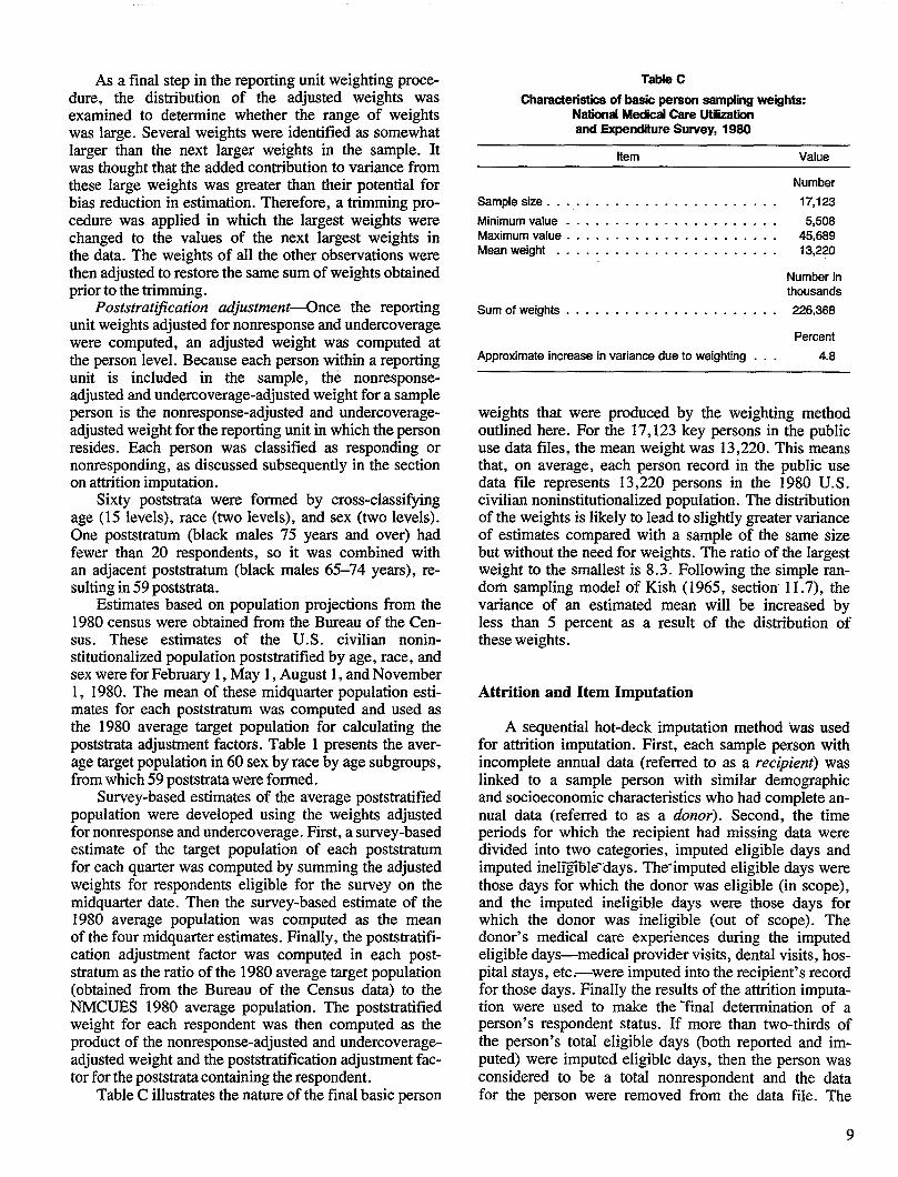
As a final step in the reporting unit weighting proce­dure, the distribution of the adjusted weights was examined to determine whether the range of weights was large. Several weights were identified as somewhat larger than the next larger weights in the sample. It was thought that the added contribution to variance from these Iarge weights was greater than their potential for bias reduction in estimation. Therefore, a trimming pro­cedure was applied in which the largest weights were changed to the values of the next largest weights in the data. The weights of all the other observations were then adjusted to restore the same sum of weights obtained prior to the trimming.

Poststratij?cation adjustment4nce the reporting unit weights adjusted for nonresponse and undercoverage were computed, an adjusted weight was computed at the person level. Because each person within a reporting unit is included in the sample, the nonresponse­adjusted and undercoverage-adjusted weight for a sample person is the nonresponse-adjusted and undercoverage­adjusted weight for the reporting unit in which the person resides. Each person was classified as responding or nonresponding, as discussed subsequently in the section on attrition imputation.

Sixty poststrata were formed by cross-classi&ing age (15 levels), race (two levels), and sex (two levels). One poststratum (black males 75 years and over) had fewer than 20 respondents, so it was combined with an adjacent poststratum (black males 65-74 years), re­sulting in 59 poststrata.

Estimates based on population projections from the 1980 census were obtained from the Bureau of the Cen­sus. These estimates of the U.S. civilian nonin­stitutionalized population poststratified by age, race, and sex were for February 1, May 1, August 1, and November 1, 1980. The mean of these midquarter population esti­mates for each poststratum was computed and used as the 1980 average target population for calculating the poststrata adjustment factors. Table 1 presents the aver-age target population in 60 sex by race by age subgroups, from which 59 poststrata were formed.

Survey-based estimates of the average poststratified population were developed using the weights adjusted for nonresponse and undercoverage. First, a survey-based estimate of the target population of each poststratum for each quarter was computed by summing the adjusted weights for respondents eligible for the survey on the midquarter date. Then the survey-based estimate of the 1980 average population was computed as the mean of the four midquarter estimates. Finally, the poststratifi­cation adjustment factor was computed in each post-stratum as the ratio of the 1980 average target population (obtained from the Bureau of the Census data) to the NMCUES 1980 average population. The poststratified weight for each respondent was then computed as the product of the nonresponse-adjusted and undercoverage­adjusted weight and the poststratification adjustment fac­tor for the poststrata containing the respondent.

Table C illustrates the nature of the final basic person

Table C

Charactenstiee of beak person sampling weight= NaticsudMedical Care Utiiition and Expenditure Sunfey, 1980

Item Value

Number

Sample size . . . . . . . . . . . . . . . . . . . . . . . . . 17,123

Minimum value . . . . . . . . . . . . . . . . . . . . . . 5,508 Maximum value . . . . . . . . . . . . . . . . . . . . . . 45,889 Meanweight . . . . . . . . . . . . . . . . . . . . . . . 13,220

Number in thousands

Sumofweights . . . . . . . . . . . . . . . . . . . . . . 226,368

Percent

Approximate increase in variance due to weighting . . . 4.8

weights that were produced by the weighting method outlined here. For the 17,123 key persons in the public use data files, the mean weight was 13,220. This means that, on average, each person record in the public use data file represents 13,220 persons in the 1980 U.S. civilian noninstitutionalized population. The distribution of the weights is likely to Iead to slightly greater variance of estimates compared with a sample of the same size but without the need for weights. The ratio of the largest weight to the smallest is 8.3. Following the simple ran­dom sampling model of Kish (1965, section’ 11.7), the variance of an estimated mean will be increased by less than 5 percent as a result of the distribution of these weights.

Attrition and Item Imputation

A sequential hot-deck imputation method was used for attrition imputation. First, each sample person with incomplete annual data (referred to as a recipient) was Iinked to a sample person with similar demographic and socioeconomic characteristics who had complete an­nual data (referred to as a donor). Second, the time periods for which the recipient had missing data were divided into two categories, imputed eligible days and imputed ineIij@e-days. The-imputed eligible days were those days for which the donor was eligible (in scope), and the imputed ineligible days were those days for which the donor was ineligible (out of scope). The donor’s medical care experiences during the imputed eIigibIe days—medical provider visits, dental visits, hos­pital stays, etc.—were imputed into the recipient’s record for those days. FinaIIy the results of the attrition imputa­tion were used to make the ‘final determination of a person’s respondent status. If more than two-thirds of the person’s totaI eligibIe days (both reported and im­puted) were imputed eligible days, then the person was considered to be a total nonrespondent and the data for the person were removed from the data file. The

9

poststratification adjustment was made after these data were removed.

The methods used to impute data for missing values were diverse and tailored to the measure requiring impu­tation. Three types of imputation predominated: Deduc­tive, sequential hot deck, and weighted sequential hot deck.

Deductive, or logical, imputations were used to fill in missing responses that could be determined readily from other data items that provided overlapping informa­tion. (These might even be referred to as edits.) For example, race was not recorded during the survey for children under 17 years of age. Instead, a logical imputa­tion made during the data processing assigned the race of the head of the household (or the head’s wife) to the child. Similarly, extensive editing was performed for the charge data before any imputations were made. For example, if first source of payment was available, only one source of payment was indicated; and if total charge was missing, the value of the first source of payment amount was assigned to the total charge item.

A 3equential hot-deck procedure (Ford, 1983) was used primarily for small numbers of imputations for demographic items. In the sequential hot-deck procedure, the data are grouped into imputation classes and then sorted within those classes by measures that are correlated with the item for which imputations are to be made. An initial value, such as the mean of the nonmissing cases for the item within the imputation class, is assigned as a “cold-deck” value. The first record in the imputation class is then examined. If it is missing, the cold-deck value replaces the missing data code. If it is real, the real value replaces the cold-deck value and becomes a hot-deck value. Then the next record is examined. Again, if the value is missing, the hot-deck value replaces the missing data code; if it is real, the hot-deck value is replaced. The process continues sequentially through the imputation classes until all missing values have been replaced.

Finally, the weighted sequential hot deck (Cox, 1980) was used most extensively, providing imputed values for a vztriety of measures, many of which had substantial amounts of item missing data. This method is a modification of the sequential hot-deck method in which the sampling weights assigned to each record determine which real values are used to impute for a particular missing value. Records are classed and sorted by measures expected to be correlated with items requir­ing imputations. The procedure is applied to several items simultaneously to reduce the number of passes of the data that are required to complete imputations on many items. Because the selection of a record to serve as a donor for a particular missing value depends on the sampling weights, it is possible for a record to serve as a donor more than one time if it has a sampling weight that is much larger than that of other records.

Often a combination of methods was used to impute for a single item. Imputations for the charge items in­

volved a combination of logical imputations, or edits, followed by the weighted hot-deck procedure. For exam­ple, an extensive edit was performed for medical visit total charges to eliminate as many inconsistencies be-tween the source of payment data and total charge items as possible. Then the medical visit records were separated into three types: emergency room, hospital outpatient department, and doctor visits. Within each type, the records were classed and sorted by different variables prior to a weighted hot-deck imputation. For instance, records for doctor visits were classified by the reason for visit, the type of doctor seen, whether work was done by a physician, and the age of the individual. Within the groups formed by these classing variables, the records were sorted by type of insurance coverage and month of visit. The weighted hot-deck procedure was used with the classed and sorted data file to impute simultaneously for missing values of total charge, sources of payment, and sources of payment amounts.

Because imputations for missing items were made for a large number of the important items in NMCUES, they can be expected to influence the results of the survey in several ways. In general, the weighted hot deck is expected to preserve the means of the nonmissing observations when those means are for the total sample or classes within which imputations were made. How-ever, means for other subgroups, particularly small sub-groups, may be changed substantially by imputation. In addition, sampling variances can be substantially un­derestimated when imputed values are used in the estima­tion process. For a variable with one-quarter of its values imputed, for instance, sampling variances based on all cases will be based on one-third more values than were actually collected in the survey for the given item; that is, the variance will be too small by a factor of at least one-third. Finally, the strength of relationships be-tween measures that received imputations can be substan­tially attenuated by the imputation.

A more complete discussion of these issues can be found later in this report.

Summary

Figure 1 is a summary of the steps in the NMCUES design from initial sample selection through the collection of data to the final weighting adjustments for nonresponse and undercoverage and imputations for item nonre­sponse. Each of these features of the survey design can have an impact on the choice of methods to use for analysis of NMCUES findings and on the interpreta­tion of results.

For example, the sampling plan, which has stratified multistage selection, requires special variance estimation procedures that account for these design features. The data collection design over the course of a l-year period leads to the consideration of average populations and estimators that resemble “risk rates” in epidemiology, with denominators that are average population estimates.

10

The imputation procedures may attenuate the strength of relationships observed from the data. The analyst (as well as the reader of reports based on NMCUES data) should be aware of the ‘implications of the design for analysis and interpretation of findings. In the next section. the nature of the public use files available to the analyst is examined.

Research Triangle Institute

Primary selection of counties and county-like units

Selection of secondary sampling units within primary selections

Selection of areas and segments within secondary sampling units

Selection of housing units within segments

I

National Opinion Research Center

Primary selection of counties and county-like units

Selection of secondary sampling units within primary selections

Selection of segments within secondary sampling units

Selection of housing units within segments

I I

Combined sample:135 primary sampling units

809 secondary sampling units and segments7,244 eligible households

6,600 responding households

Round 1 data collectionFebruaty-April 1980

Personal visit interviewSupplement interview

(16,902 responding key persons)

I Egure 1

Overview of design of National Medii Care LJtikzationand Expendtire

I

Survey 1980

11

IRound 2 data collection

May-July 1980 Personal visit interview

Round 3 data collectionAugust-October 1980Telephone interview

Supplement interview

Round 4 data collectionNovember-December 1980

Telephone interviewApproximately 2/3 ofsample interviewed

Round 5 data collectionJanuary-March 1981

Personal visit interviewSupplement interview

Data collection and processingReceipt control system

Manual edit, coding, keypunching

Analytic file construction Machine edit, recoding

Sampling weights Attrition/item imputation

Figure 1

Overview of design of National Medical Care Utiliition and Expenditure Survey 1980-Con.

12

Public Use Data Files

Overview and Data Management Considerations

The NMCUES national household survey public use data files comprise six fixed-length rectangular files dis­tributed on six magnetic tapes. The files are labeled as follows: Person, medical visit, dental visit, hospital stay, prescribed medicine and other medical expenses, and condition. Depending on the type of analysis re­quired, the user may need to create various analytic files by combining information from these different files.

The pivotal data file is the person file, which contains a primary record of information for each of the 17,123 key individuals in NMCUES. Sampling weights for all of these individuals are recorded only in this file. All other data files contain medical event or condition records only for individuals reporting medical events or condi­tions; that is, the medical event files contain information, including sampling weights, only for users of the service covered in the file. Similarly, the condition file contains information only about persons reporting conditions that resulted in health care use and/or disability. Therefore, these files must be linked with the person file for any analyses on the individual level that include persons whose records are available only on the person file.

A study of different sources of payment for all health services, for example, requires manipulation of several data files. Data must first be aggregated for each person across the various medical event files, taking into account the specific source of payment for each event. The source-of-payment data can then be linked through the participant sequence number with information in the per-son file to produce source-of-payment estimates by vari­ous individual characteristics. Thi’smanipulation of files for source-of-payment data is necessary for three reasons. First, source-of-payment data are not available on the person file; only annual total charges for each type of service are available from the person file records. Sec­ond, data must be aggregated across different types of use for each individual. Third, the medical event files cannot be used to produce individual-level estimates. for the total sample population (includlng nonusers of one or more types of service) independent of the person file because data for nonusers are not included on the event files.

Source-of-payment estimates for users of a specific type of service only, such as hospital care, can be pro­duced using the relevant medical event file alone. Event-Ievel estimates, such as charges by source of payment

for hospital stays, can also be produced without linking to the person file.

Condhion-specific analyses, such as those reported in Murt et al. (1986), Harlan et al. (1986), and Harlan et al. (to be pubIished), require sophisticated manipula­tion of the data iles because the various files are or­ganized around different types of records and contain overlapping information.

The person file contains only summary information about conditions, medical events, and disability. A count of the number of condkions and some information about activity limitations and disabling conditions are included, but no information is given for linking conditions with specific events or disability days. Annual totals for use of and charges for the various types of health services and totals for disability days are also listed. The person tle does not include source-of-payment data. However, it does include information about health care coverage and a variety of other health-related variables, such as usual source of care, as well as a full range of demo-graphic and socioeconomic characteristics.

In the condition file, a specific condition is the unit around which all other data in the file are organized. Each reported condhion is assigned a unique condition number, and the information concerning each condition is recorded on a separate record. The 51,465 records in the condition file include only conditions that resulted in disability and/or use of health services. Charges for health services are also associated with each condition, as are reasons for not seekkg medical care and month and year of onset or accident.

It should be noted that respondents or informants were allowed to report more than one condition for each medical event or episode of disability days. No primary condition was indicated when multiple condi­tions were reported. AI] charges, use of service, and disability were associated with each reported condition. For example, all charges for a particular hospital stay are assigned to each condition reported for that hospital stay. Therefore, summation of use, charge, and disability data from the condition file results in a duplicated count of these measures on the person level of analysis; that is, one disability day would be counted twice for one person if two conditions were listed as causing that disability day.

In contrast, the varioui medical event files (hospital stay, medical visit, etc.) are organized around individual events. Each reported medical event is assigned a unique

13

number, and the information concerning each medical event is recorded on a separate record. In the medical event files, conditions, charges, and sources of payment, but not disability, are associated with each medical event. (Conditions are not associated with dental visits.) Indi­vidual-level analysis of medical event data requires link-age with the person file if nonusers are to be included in the analysis or if more than one type of service is being studied. There are 86,594 records in the medical visit file, 23,113 records in the dental visit file, 2,946 records in the hospital stay file, and 58,544 records in the prescribed medicines and other medical expenses file.

Imputation status is recorded on all six files for all variables included in NMCUES imputation procedures.

Analysis of condition-related data at the person level requires linkage at least between the condition and person files and may require linkage with one or more of the medical event files as well. Estimation of disability days for persons reporting neoplasms, for example, requires Iinkagebetween the condition and person files. An analy­sis of sources of payment for hospital and physician services for persons reporting neoplasms would require additional linkage with medical visit and hospital stay files.

In any person-level analysis of data from the condi­tion file, the possibility of reporting multiple conditions must be taken into account, as noted earlier. Multiple counting of charges or disability days maybe permissible for condition-level analysis. However, to avoid multiple counting, person-level anal ysis may require apportion­ment of charges or disability days among the various conditions reported for the same medical event or disabil­ity episode. Attribution of all charges or disability days to one of the reported conditions is another alternative. Because no primary condition is specified, assignment of all charges or disability days to the first condition listed may be the best option if the latter approach is selected.

Data Modifications

A number of data accuracy problems in the NMCUES public use files require modification before data analyses are conducted. Most of these modifications have some relationship to the hospital file; that is, changes must be made to variables in the hospital stay file or to hospital-related summary variables that appear in the person file. Other modifications involve newborn sampling weights, disability days, health care coverage, and categorical poverty status. Analyses that do not require the use of the hospital stay file and/or hospital-related variables in the person file or the other variables listed here can be performed without making these modifications.

The following problems were identified and ad-dressed by modif ying the data files.

(1) Sampling weights for ’68 newborns were changed to reflect accurate survey eligibility status in accord-

14

ante with instructions from the National Center for Health Statistics.

(2) Hospital charges were corrected for six respondents with, extremely high values.

(3) Forty-seven respondents were reassigned to appropri­ate health care coverage categories based on source-of-payment data.

(4) Records for 175 persons had fewer bed-disability days than hospital nights. Records were edited to make the number of bed-disability days equal to the number of hospital nights.

(5) Coding errors were corrected for four respondents with incorrect hospital admission or discharge dates.

(6) Poverty status classification on the categorical vari­able was inconsistent with the continuous poverty status variable for four respondents. Categorical as­signments were changed for those four individuals.

(7) A number of changes were necessary to correct infor­mation about nine respondents whose hospital records were incorrectly coded as deliveries in the hospital file.

(8) Hospital records were modified for one respondent who had duplicate records.

Newborns

Sixty-eight newborns were incorrectly considered eligible for the entire survey period. These errors were corrected by changing the eligible time-adjustment factor and the person time-adjusted weight for each of the 68 records. Table 2 presents the person identifying ‘ number (or participant sequence number) and revisions to time-adjusted weights and time-adjustment factors for these 68 newborns.

Hospital Stay Charges

Six hospital stay records with total charges of $90,000 or more contained the highest charges for indi­vidual medical events recorded in the NMCUES data files. Because of their importance to estimates of total charges and other expenditure measures, these records were carefully reviewed by University of Michigan and National Center for Health Statistics personnel. Several inconsistencies within these records suggested that the charge data were incorrect and required revision. These six records and related information in the person file were changed to conform with Medicare records main: tained by the Health Care Financing Administration or with other information about each of the six hospital stays. In several cases, examination of Medicare records revealed that the error in the NMCUES hospital file resulted from a miskeyed decimal place. Table 3 presents the revised values in the hospital stay file, and Ta­ble 4 presents the revised values in the person file for these six records.

Health Care Coverage

Discrepancies between source of payment and health care coverage were noted in the course of analysis of the NMCUES data. All of the discrepancies involved Medicare coverage. Forty-seven respondents reporting Medicare as a source of payment in the medical visit, hospital stay, or prescribed medicine files were not prop­erly coded as covered by Medicare. Health care coverage for these respondents was reclassified strictly according to source-of-payment data, except as follows.

� Respondents originally coded as covered by private insurance but not showing private insurance as a source of payment for any services were coded as having Medicare and private insurance coverage.

� For cases in which reassignment based on imputed data would conflict with reassignment based on real data, the real data were used.

The original and revised health care coverage categories for these 47 persons are presented in Ta­ble 5. Both categories are based on health care coverage definitions developed by the University of Michigan re-search staff and reviewed by the National Center for Health Statistics project staff. Although the University of Michigan health care coverage variables were derived from information on the public use files, these coverage categories are not dhectly available on the public use files. Therefore, if the University of Michigan categories are not used, other changes must be made to the health care coverage variables that are on the person file for respondents listed in Table 5. Information about those changes can be obtained directly from the Utilization and Expenditure Statistics Branch, Division of Health Interview Statistics, National Center for Health Statistics. The University of Michigan health care coverage categories are mutually exclusive and are specified as follows.

Under 65 years

Coverage all year: Private insurance only Medicaid only Other public program only

Mixed coverage: Private insurance and public program More than one public program

Part-year coverage No coverage

65 years and over

Medicare coverage: Medicare only Medicare and private insurance Medicare and other public program

No Medicare coverage~ Any other coverage No coverage

Specific codes for these categories are presented in Tables 6and7.

Bed-Disability Days, Restricted-Activity Days, and Hospital N]ghts

Examination of values for hospital nights and bed-disability days revealed that in 175 cases the value for hospital nights was greater than the value for bed-disabil­ity days (Table 8). According to interviewer instructions for the NMCUES que$ionnaire, hospital nights should be included in bed-disability days, except for newborns. Therefore, the vaIue of bed-disability days was revised to equal hospital nights for these 175 cases. Restricted-activity days were also revised to reflect the added bed-disability days. This adjustment is a standard edit for this type of inconsistency in a data set. However, it does not fully compensate for errors in recording or computing bed-disability days. Bed-dkabllity days are probably underestimated even after the revision. The edit was performed without regard to the imputation status of either bed-disability days or hospital nights.

Hospital Admission or Discharge Dates

Four cases identified in the examination of discrepan­cies between hospital nights and bed-disability days were discovered to have improperly coded hospital admission or discharge dates. Lengths of hospital stay were incor­rectly coded for these cases. The admission or discharge dates and hospital nights were corrected for these four cases, but bed-disability days and restricted-activity days were not altered (Table 9).

Poverty Status

Cross-tabulation of poverty status classification de-rived from the continuous variable by poverty status categories coded on the public use files indicated that four respondents.were miscoded on the categorical vari­able. The categorical variable for these four respondents was recoded to agree with poverty status on the continu­ous variable (Table 10).

Deliveries

Problems were discovered cm nine records coded as deliveries in the hospital stay file. A variety of resolu­tions were identified as appropriate.

� Two deliveries were attributed to male respondents. Examination of individual records suggested that the sex variable was incorrectly coded in these two cases. The sex variable was therefore recoded to female.

15

� A third delivery attributed to a male was actually that of the respondent’s spouse. In this case, the hospital record was reassigned and appropriate changes made in the person file for both persons.

� Four hospital stays for newborns were incorrectly coded as deliveries., These were recoded as newborn stays in the hospital stay file.

� A fifth newborn’s hospital record was attributed to its mother. In this case, the hospital record was transferred to the newborn, and appropriate changes were made in the person file for both persons.

� One delivery was attributed to a woman 74 years of age. Following advice from the National Center for Health Statistics, the record was recoded to reflect “signs, symptoms, and ill-defined conditions” as the admitting condition.

These changes are summarized in Tables 11 and 12.

Duplicate Hospital Stay Records

Two sets of duplicate records (four records in total) in the hospital file were discovered for one respondent. The two duplicates were deleted in the hospital stay file, and necessary changes were made in the person file. Three of the four records had been imputed to another respondent as part of the attrition imputation process. No changes were made in the records for the person receiving the imputations. These modifications are presented in Table 13.

16

Effects of Imputation on Survey Estimates

The effects of imputation on survey analysis initially do not appear to be a concern because, when imputation occurs, the number of items and the amount of imputation for any given item are usually limited. Moreover, these effects can be misleading because it appears that the data are complete and’ that no special procedures are needed to compensate for missing data in the analysis, when in fact the imputed values can have substantial effects on survey estimates (Dempster and Rubin, 1983). For the analyst aware that imputation Wcumed for miss­ing data for a particular item, it certainly is easier to assume that the effect of imputation on a particular analy­sis can be ignored safely or that the effect is completely beneficial (i.e., reduction of bias resulting from missing data). Unfortunately, for some types of items in a survey data set, the amount of item nonresponse and imputation can be substantial, producing large effects on the results of the data analysis.

In the section on survey design, the extent of missing data in NMCUES and the methods used to compensate for missing data were discussed. Imputation procedures that were used to compensate for item nonresponse were also reviewed. The purpose of this section is twofold: To examine the effects of imputed values on the analysis of NMCUES data and to review analytic strategies that might be used to handle imputed data. We begin by reviewing analyses for several utilization and expenditure measures with and without imputed values included in the computations. Based on these investigations, several strategies available for handling the imputed data in the statistical analysis are suggested. Finally, recommen­dations are made about suitable strategies for the routine analysis of NMCUES data with imputed values.

Empirical Findings

Extensive imputations were made for missing values for a large number of the key items in NMCUES. Imputa­tion can be expected to influence estimates made from the survey in several ways.

Although the weighted hot deck is expected to pre-serve the means of nonmissin~ observations for the total sample or classes within whi~h imputations were made (Cox, 1980), this will not be the case for sampling variances. Sampling variances can be underestimated

substantially when imputed values are used in the estima­tion process (Kalton and Kasprzyk, 1982). For example, the estimated sampling variance for a variable with one-quarter of its values imputed will be based on one-third more values than were actually collected in the survey when the computations include all the data, real as well as imputed values. Thus the variance will be underesti­mated by a factor of at least one-third (Kak%i, 1983).

Relationships observed among variables based on the real values can be altered significantly when imputed values are included in the analysis. In particular, the strength of a relationship may be attenuated by imputa­tion. Santos (1981) demonstrates that the attenuation of correlations by imputed values can be substantial.

Table 14 presents estimated means and sampling errors for five survey measures from NMCUES that have smrdl to modest levels of missing data (from 8 to 18 percent). Separate estimates are presented for com­putations using all data (both real and imputed) and using only the real data for each measure. The weighted mean and its standard error can be computed under two different assumptions. The simple random sampling (SRS) standard error of the mean is computed as though the observations were selected independently, but the sampling weights are included as part of the estimate. The weighted complex standard error accounts for the stratified multistage nature of the design, including the weights. The ratio of the complex to the SRS sthndard error is the square root of the design effect. (The design effect is the ratio of the variances. ) This ratio is presented in the last column of Table 14. The design effect fre­quently is used to assess the effect of the sample design on survey estimates. It is generally found to be greater than 1for complex sample surveys.

For each disability measure in Table 14, the means computed using all the data and using only the real data are quite similar. ~is similarity is expected because the weighted hot-deck imputation procedure is designed o preserve the weighted mean for overall sample esti­

mates. However, the SRS standard errors are smaller when all the data are used. The SRS variance is inversely related to the sample size; therefore, imputed values increase the number of observations used in the variance calculation. Similarly, the complex standard errors for bed-disability and work-loss days are smaller when all the data are used. At the same time, the ratio of th&

17

complex to SRS standard error essentially remains un­changed whether only real or all data are used. The decrease in the standard error when all data, instead of only real data, are used is proportionately the same for the SRS and the complex standard errors, except that the complex standard error for cut-down days and restricted-activity days is slightly larger when all the data are used.

One may conclude that imputation for the disability measures shown in Table 14 has little or no effect on estimated means or their standard errors. Although these results were computed for the total population, similar findings may be expected for most subgroups.

In contrast, imputation has larger effects for measures that have more extensive amounts of missing data. For example, more than one-half of the entries for total charge for a hospital outpatient department visit were missing. (See Table 15.) Of 9,529 hospital outpatient department visits (real visit records plus those generated from the attrition imputation process), 4,841 have a total charge that was imputed from one of the other hospital outpatient department visit records. Thus, 50.8 percent of the total charges were missing for this particu­lar medical event. Despite the large amount of missing data, the weighted means computed using all the data and using only real values are similar, although the mean for all the data is slightly lower.

Table 15 also presents the means and other estimates for real data by the number of times a record was used as a donor in the weighted hot-deck imputation process. Donor records were chosen within classes in which the donor and imputed record were similar. Therefore, donors and recipients should have similar values for the measure being imputed. However, based on donor group means in Table 15, it appears that outpatient de­partment visits with missing values received quite differ­ent mean total charges from those without missing values. On average across all donor classes, the visits with missing values received imputed values with lower mean total charges than the charges for real values.

It is also shown in Table 15 that sampling errors are changed substantially when imputed values are added to real values in the computation. The SRS standard error decreases 28.8 percent when the imputed values are added to the computation. Because the SRS variance (the square of the SRS standard error) is inversely propor­tional to the number of observations used in the calcula­tion, it is expected to decrease by the proportionate reduction in sample size (50.8 percent). However, the SRS variance actually decreases by 49.3 percent, suggesting that sample size alone does not account for the magnitude of the observed reduction. This difference between expected and observed decrease in sampling variance is small and may be attributable to variability in the imputation process itself. Nevertheless, it is of interest to investigate the extent to which the amount of variability among elements may also be increasing when imputed values are added to the calculation.

An estimate of the element standard deviation, a

‘measure of the variability among elements, was com­puted by multiplying the SRS standard error by the square root of the sample size. The estimated element standard deviations are presented in the last column of Table 15. The element standard deviation actually in-creases by 2.6 percent when imputed values are included. The expected decrease in standard error is reduced by this change in element variance. Furthermore, an exami­nation of the element standard deviations for the various donor subgroups indicates that donors had greater varia­bility with respect to outpatient department visits than did the total group with real values (which includes the donors).

The decrease in the SRS standard error when using all data is somewhat smaller than expected given the increased sample size, but the decrease in the complex standard error is actually larger than might be expected. The complex standard errors decreased 34.8 percent rather than 29.9 percent, the expected decrease based on sample size alone. A,s a result, the ratio of complex to SRS standard errors decreases somewhat wlen im­puted values are included. This larger than expected decrease probably results from the imputation of values across strata and primary sampling units that are used to form computing units for complex variance estimation. Imputation across computing units has the effect of de-creasing the variability among units and reducing the computed standard error.

Neither the complex standard error computed using only real data nor the one computed using all data is the actual standard error of the weighted mean computed using all the data. The mean computed using all data includes 4,841 values that were actually subsampled with replacement from the 4,688 real values. In addition, the imputations were made across the strata and primary sampling units used in the complex variance estimation procedure, a process which requires an assumption that the observations are seIected independently between pri­mary sampling units and strata. Hence, the complex standard error based on computations using all the data, shown in Table 15, fails to account for two sources of variability: The double sampling used to select values for imputation and the correlation between primary sam­pling units and strata induced by imputation.

At the same time, the complex standard error for the weighted mean computed using only the real data is an incorrect estimate of the standard error of the mean based on all the data. The actual standard error of the weighted mean computed using all the data is probably larger than that shown in Table 15. It may even be larger than the standard error computed using only the real data.

Unfortunately, none of the estimators used in Table 15 is totally appropriate for the actual standard error for the weighted mean computed using all the data. An appropriate estimator might be developed if informa­tion about the correspondence between a specific donor and recipient were available, but this information is not usually provided on public use tapes of survey data.

.-

18

As an alternative, an estimation strategy was developed based on an adjustment to the sampling weights to com­pensate for item missing data rather than making use of the imputation process results.

The first step in the adjustment of sampling weights to compensate for item nonresponse for outpatient depart­ment visits is the creation of the original imputation classes. Sixteen classes were formed by cross-classifying age (under 17 years, 17-44 years, 45-64 years, and 65 years and older), sex, and whether or not a doctor was seen during the visit. Within each class, weights for recipients of an imputation were summed, and the total number of donations made in the class was counted. The sum of the weights for imputed records was then divided by the number of donations within each class to form an average weight that each donor contributed to an imputation within the class. In the final step in the process, the person weight for each donor was in-creased by the average donor weight multiplied by the number of donations in the imputation process for outpa­tient department visits made by that particular donor. These adjusted weights for donors have the property that they sum, within an imputation class as well as over all classes, to the total sum of weights for donors and recipients combined.

The adjusted weights permit the estimation of a mean or other statistic using only the real data as well as incorporation of an adjustment for item nonresponse di­rectly into the estimate. Moreover, correct complex standard errors can be computed for these weighted means using the real data and the adjusted weights be-cause imputation across strata and primary sampling units does not occur.

The estimated mean and its standard error under this adjusted weighting procedure, shown in the last row of Table 15, are similar to those obtained using all the data. However, they are greater than those ob­tained using only the real data with unadjusted weights and those obtained using all the data. The difference between the complex standard error for the weighted mean computed using only the real data and for the mean computed using adjusted weights is caused by the effects of increased variability of adjusted weights relative to the unadjusted weights.

As a final illustration of the effects that imputation can have on survey data analysis, the relationship be-tween total charges for outpatient department visits and family income of the person making the visit is examined. Figure 2 presents estimated mean total charges per outpa­tient department visit computed using all the data and using only the real data for four family income groups. Using only the real data, the mean total charge per visit increases linearly as the family income increases. However, when all the data are used to estimate the mean total charge per visit, the mean charge does not increase as rapidly with increasing family income. This linear relationship between family income level and mean total charge per outpatient department visit in the real data has been attenuated by the imputed values. Table

Datatype� All•l Real P

/

,/’

cf-35~

Lessthan $5,000- $12,000- $35,000 $5,000 $11,989 $34,999 or more

Familyincome

Fgure 2

Mean charge for hospital outpatknt department visits, by income group: National Medical Care Utilization

end Expenditure Survey, 1980

. Data type , All

- 0 Familyincome P lessthan $5,000

:

I 1 I I I I 1 I .j#+’ 1 I I I 1 [ 1 2345 678 910111213141516

Imputationclass

F~ure 3

Mean charge for hospital outpatient department visits, using real date only, by imputation CISSS National Med~

Care Utiiizetkm and Expenditure Survey, 1980

16 presents the mean total charges for each of the four income groups for all data and for only the real data.

The reason for this attenuation can be deduced from Figure 3. Sixteen imputation classes—based on measures that did not include family income—were formed” for the imputation of total charges for outpatient department visits. Figure 3 shows mean total charges for real data for the total sample and the subgroup with family income less than $5,000 in 1980.

19

The low-income group generally has lower mean charges than the total sample has. However, family in-come was not one of the variables used to form imputation ~lasses. Therefore, low-family-income persons within an imputation class with missing outpatient department visit total charges were imputed a charge that was, on average, higher than the mean charge for low-income persons with real data. This occurred in almost every imputation class. When the real and imputed data for persons with family incomes less than $5,000 are com­bined, the effect of imputation is to increase the mean charge for this subgroup. Conversely, for persons with family incomes of $35,000 or more, total outpatient department visit charges for persons with real data tend to be larger than values imputed to persons with missing charges. The overall impact of the imputation process on the relationship between charges for outpatient depart­ment visits and family income is a regression toward the mean charge for real data for low- and high-income subgroups.

Thjs attenuation occurs when the subgroups are formed from a measure that was not controlled for in the imputation process for the item receiving imputations. In addition, the relationship will not be attenuated as seriously if only real data and adjusted weights are used in the analysis, as shown in Table 16.

Strategies for Imputed Data

The results presented here demonstrate the effect that imputation can have on estimated means, estimated standard errors, and relationships among measures. The analyst of the NMCUES data must select a strategy for handling imputation in estimation. The results in this section allow comparison among four different strate­gies for handling imputations in the NMCUES data

(1) Use all the data, real as well as imputed, in all analyses.

(2) For each item with missing data, create weights that adjust ,for the item missing data and use only the real ddta with adjusted weights in all analyses.

(3) Use only the real data with unadjusted sampling weights (i.e., ignore the effects of item missing data) in all analyses.

(4) Use an adaptive strategy, selecting Strategy 1 or 3 depending on the type of analysis to-becond~cted.

These strategies were examined for a series of analyses of the NMCUES data (Berki et al., 1985; Par-sons et al., 1986). We considered each strategy with respect to three criteria:

� The practicality of implementing the strategy without developing special-purpose software for analysis.

� The accuracy of estimates of totals or aggregates, means, and standard errors of means.

� The degree of attenuation of relationships between two measures attributable to the strategy.

20

After reviewing findings similar to those presented in this report, we chose to follow an enhanced version of Strategy 1. It is useful to examine the practicality and accuracy criteria for each strategy in the specific context of analysis of the NMCUES public use data and the weighted sequential hot-deck imputation proce­dure used for those data.

Strategy 1 is practical to implement because no spe­cial adjustments to standard analytic methods are neces­sary. Estimates of aggregates or totals (such as total charges for outpatient department visits) are automati­cally adjusted for the failure to obtain responses from some persons, and weighted means for the total sample are similar to those obtained by using only the real data. However, standard errors estimated using all the data and standard variance estimation techniques will , tend to underestimate the actual standard errors, the severity of the underestimate depending primarily on the amount of imputed data. Moreover, relationships between imputed measures and variables not used as control variables in the imputation process can be at­tenuated. Strategy 1 can be enhanced by presenting esti­mates of standard errors with an indication that some estimates may be subject to substantial underestimation because of imputation. In addition, multivariable analyses should be conducted both with and without imputed values to assess the impact of imputation.

In contrast to Strategy 1, Strategy 2 is not practical to implement. It would be a sizable task to create adjusted weights for each item used in a large-scale analysis. In addition, the choice of an estimation procedure for a multivariable analysis involving two or more measures, each with a different weight, is not obvious. The advan­tage of the adjusted weight strategy is that standard errors could be estimated for estimated means “tising standard estimation procedures applied to the real data with adjusted weights. In addition, weighted means com­puted using only the real data would essentially be identi­cal to those computed using all the data, estimated totals would not be subject to underestimation because of item missing data, and the strength of relationships among survey measures would not be as seriously attenuated asunder Strategy 1.

Strategy 3, like Strategy 1, is practical to implement, although some recoding of data items may be necessary on most statistical software systems to identify imputed values as missing rather than real. The weighted means for the total sample provided by Strategy 3 do not differ substantially from those estimated using all the data. Standard errors can be estimated for these real data means, and relationships among survey measures will not be attenuated by the imputation process. However, estimated totals for items with substantial amounts of missing data will be severe underestimates if only real data are used.

Analysts employing the final adaptive strategy might use only the real data to estimate means and their standard errors and to analyze relationships among survey meas­ures. Estimates of totals would be computed using all

the-data to avoid severe underestimation for survey meas­ures with large rates of item missing data. Under Strategy 4, one still would be faced with the estimation of standard errors for totals for which imputed values were used; a suitable standard error estimation procedure is not readily available for sample survey data that have values imputed across strata and primary sampling units. For the most part, an adaptive strategy is practical to imple­ment because it does not require any particular analyses that cannot be done using standard statistical software. However, extensive analysis of a large survey data set may be cumbersome when analytic methods are tailored to the amount of item missing data for measures used in the analysis.

Strategy 2 cannot be recommended because it is impractical to make item missing data adjustments to weights for the numerous estimates needing adjustment. Moreover, it is difficult to use the adjusted weights in multivariable analysis. Similarly, for routine analysis of survey data, Strategy 3 cannot be recommended be-cause of the potential for highly inaccurate and mislead­ing estimation in analysis.

For analysis of surveys that are smaller and less complex than NMCUES and that involve a limited number of analyses, Strategy 4 may be a feasible altern­ative. For smaller analytic tasks, greater attention can be given to refinements that may improve the accuracy of the reported results. Clearly Strategy 4 cannot be recommended when the size or complexity of the analytic task increases.

For a large complex survey such as NMCUES, we recommend that Strategy 1be followed. However, signif­icant attention must be given to investigating the effects of imputation on analysis. In particular, analysts should

familiarize themselves with rates of item missing data for key survey items and the imputation methods used to compensate for missing data. For items with significant amounts of missing data, estimates of means, totals, and standard errors ought to be made both with and without imputed values to assess the effects of imputation on those estimates. Similarly, analyses of substantively important relationships should be conducted both with and without imputed values to assess whether imputation is seriously attenuating the strength of the observed relationship.

When this enhanced form of Strategy 1 was used in analyses of NMCUES data, the analytic task was increased by the need to conduct some analyses both with and without imputed values. However, the increased burden was reduced somewhat by careful selection of the types of measures for which both types of estimates were computed and by identifying the relationships that were substantively most important, for which an assess­ment of the effects of imputation was needed.

The results of investigations of the effects of imputa­tion on analysis may cause the alteration of the presenta­tion and interpretation of findings. Standard errors for estimates that are based on measures with substantial amounts of imputation can be indicated in tabular or other types of presentations. This approach may not be feasible in many cases. If it is not feasible, reports on analytic findings must at least include warnings to the reader that estimates of standard errors for some measures may be substantial underestimates because of imputed values. Thus, the interpretation of analytic find­ings concerning relationships among survey measures. can be informed and guided by knowledge about the impact of imputation on results.

21

� �

�

Estimation Methods

Notion of an Average Population

NMCUES was a panel survey in which members of the population were followed during the panel period (calendar year 1980). The nature of a dynamic population over time influences the rules used to determine who should be followed and for how long. It also has signifi­cant implications for the form of estimators for character­istics of the population during the panel period. Before discussing estimation strategies for the NMCUES data, it is useful to review the nature of a dynamic population over time.

Figure 4 illustrates the nature of a longitudinal popu­lation as members move in and out of eligibility. Stable members of the population appezu-at the beginning and at every time point during the life of the longitudinal time period. Even though these persons are termed “stable,” they may of course change residence during the panel period and may be quite diftlcult to trace. They may even be lost to followup during the course of the panel, but as long as they remain in the population, they are referred to as stable population members. Leav­ers are persons who are eligible at the beginning of a time period but become ineligible at some later time. Leaving may occur through events such as death, in­stitutionalization, or moving outside the geographic boundary of the population. Those lost to followup are not leavers. At the same time, new members (entrants) may enter the population through births or through returns from institution? qifrom outside the geographic boundary of the population. Finally, there also will be population elements that are both entrants and leavers from the population during different time periods. The majority of the population typically will be stable in nature, but it is the entrants and leavers, persons who may be ex­periencing major changes in their lives, who are often of particular interest to analysts of panel survey data. In order to assure adequate coverage of all elements in the dynamic population considered over the entire time period, ~“CUES followup rules were carefully specified to properly include entrants, leavers, and mixed population elements.

As an illustration, consider a person who was in the Armed Forces on January 1, 1980, was discharged on June 1, 1980, and then became a key person (i.e., one to be followed for the rest of the year while eligible) in the NMCUES panel. Because NMCUES was designed

Stable

b

Leaver

b

F

Entrant

b

Mixed

*

~~

O 1 23 4 56789101112 Time

Figure 4

Dynamic populetkrn for 12 time *nod panel survey

to provide information about the civilian population, medical care use and charges for, this person during the first 5 months ,of 1980 are dutside the scope of ttie survey. Data about health care use and charges were not collected unless they occurred after June 1. At the same time, this person was eligible for only 7 months of the year, and he was also ‘tat risk” of incurring health care use or charges for only 7 of the 12 months. This person thus contributes only 771,2, or 0.58, of a year of eligibility, or “person risk,” to the study. This quantity is referred to as the “time-adjustment factor” in the NMCUES documentation and in this report.

For readers not familiar with the concept of “person years of risk,” it may be useful to consider briefly the rules that were used to determine eligibility for a given person at a given moment during 1980.. ‘There were essentially two ways of becoming eligible for or entering the NMCXJESeligible population. The obvious way was

22

to be a member of the U.S. civilian noninstitutionalized population on January 1, 1980, and hence to be a member of the original, or base, cohort about which inferences were to be made. The second way to become a member of the eligible population was to enter after January 1 through birth or through rejoining the civilian nonin­stitutionalized population during the year by returning from an institution, from the Armed Forces, or from outside the United States. There were also se~@ ways by which persons who were eligible members of the population could become ineligible. Death obviodly re-moves a person from further followup, as does in­stitutionalization, joining the Armed Forces, or moving to a residence outside the United States. Information was collected to monitor the exact number of days that each person selected for NMCUES was eligible duriing the year. These eligibility periods are summarized by the time-adjustment factor on each record.

The use of “person years” to form sample estimates requires careful assessment of the characteristic to be estimated. Estimates that use only data collected from persons during periods of eligibility (e.g., total number of doctor visits or total charges for heahh care) do not need to account for time adjustments. Estimates for per-son characteristics (e.g., total population or proportion of the population in a given subgroup) must be based on person years to obtain estimates that correspond to the desired target population quantities. Some estimates require the use of the time-adjustment factor in the de-nominator but not in the numerator. For example, an estimate of the mean total charge per person for health care during 1980 must use the total charges for health care as a numerator without time adjustment. However, the denominator must be the number of person years that the U.S. population was exposed to the risk of such charges during 1980, a time-adjusted, or person-years, measure. The mean in this case is actually a rate of health care charges per person year of exposure for the eligible population in 1980.

When making estimates in which person years are important, the effect of the time-adjustment factor will vary depending on the subpopulation of interest, as can be noted in Table D. A cross-sectional cohort of JV persons selected from the U.S. population on January 1, 1980, and followed for the entire year will contribute a total number of person years for 1980 that is smaller than N because of removals such as deaths or in­stitutionalization. If entrants are added to the initial cohort during the year, the person years contributed by the initial cohort and the entrants may well exceed N, but it will still be less than the number of original cohort members plus the number of entrants.

The difference between persons and person years will vary by subgroups as well. Females 25–29 years of age on January 1 constitute a cohort for which few additions are expected because of entrants from institu­tions, the Armed Forces, or living abroad. Few removals are expected because of death, institutionalization, join­ing the Armed Forces, or moving abroad. On the other

Table D

Effect of person-year adjustment on counts andaampHngweighta for selected population groups:

National Medieel Care Utiiiition and Expendfiure Survey, 1980

Sample Person Sampling weight

Population group size yeara Basic Adjusted

Number in Number thousands

Total population . . . . . . . 17,12316,862.84 226,368 222,824

Female, 25-29 years . . . . 702 699.39 9,529 9,494

Male, 80 years and over . . 113 104.05 1,384 1,274

All persons born during 1980 . . . . . . . . 251 121.02 3,560 1,713

hand, males 80 years of age and over on January 1 will contribute a much smaller number of person years to the population than the total number of persons in the cohort at the beginning of the year, because a large number of the cohort will die or become institutionalized during the year.

Estimation Procedures

Sample estimators from the NMCUES data, regard-less of whether they are totals, means, proportions, stand­ard errors, or some other estimator, must account for the complexity of the sample survey design. Totals, means, and other estimates must include sampling weights to compensate for unequal probabilities of selec­tion, nonresponse, and undercoverage. Stratification, clustering, and weighting must also be accounted for in the estimation of sampling errors. In addition, one must consider time-adjustment factors to account for persons not eligible for the entire year and imputations that were made to compensate for missing items. These factors all affect the precision and accuracy of the sample estimators to some extent, as discussed previously.

In NMCUES, a stratified multistage probability sam­ple design was used to select the initial sample of report­ing units followed in the survey. The stratification and clustered sample selection, as well as weighting adjust­ments, must be accounted for in the calculation of esti­mates. As described previously, the NMCUES sample design involved up to four stages of sample selection and stratification for each of those stages. It would be difllcult to incorporate the full complexity of this sample design into estimation procedures.

Fortunately, it is not necessary to incorporate the full complexity of the design into the estimation proce­dures in order to obtain valid estimates of totals, means, standard errors, and other estimates. RTI has provided codes with the NMCUES data files that can be used to estimate various quantities of i;terest in a practical manner. Nonetheless, the estimation procedures for NMCUES are still complicated, and added notation is required to reflect speciaI considerations needed in estimation.

23

For the NMCUES estimates, individuals are indexed by stratum, by primary sampling unit within stratum, and by individual within primary sampling unit. Codes are provided in the data set to identify the stratum and primary sampling unit for each person record. They are referred to in the public use data tape documentation as the pseudostratum and pseudoreplicate codes. The term “pseudo” is used because these codes do not corre­spond exactly with the strata and primary sampling units used in sample selection. In order to simplify subsequent variance estimation procedures, the NMCUES sampling statisticians grouped strata and primary sampling units used in the sample designs from the two survey organiza­tions. For example, the actual sample selection may have involved such procedures as the selection of a single primary sampling unit within a stratum, but for purposes of variance estimation, strata have been col­lapsed such that exactly two primary sampling units are in a pseudo, or collapsed, stratum. There are 69 pseudostrata, each with exactly 2 pseudo-primary sam­pling units orpseudoreplicates, in NMCUES.

Let h denote the pseudostratum or stratum for each person in the NMCUES data set, where h = 1,,.., 69. Let a denote the pseudoreplicate within a particular stratum, where a = 1 or 2 only. Finally, let k denote the individual within a particular pseudoreplicate and pseudostratum, where k = 1,..., nh. (The number of persons within pseudoreplicates varies across pseudorep-Iicates.) The (hak)th individual is uniquely identified by the pseudostratum and pseudoreplicate codes and a person-level code within those units.

A variety of estimators can be formulated from NMCUES data, depending on the focus of the analyses. To illustrate the role of time adjustments, weights, and other aspects of forming estimates for NMCUES, consid­er six estimates that appear in NMCUES reports:

(1) An estimated total charge for a selected subgroup, such as persons below the poverty level.

(2) An estimated total population, such as the number of females.

(3) The mean charge per visit.

(4) The mean charge per person.

(5) The proportion of persons whose charge is less than or equal to a fixed level.

(6) The proportion of all charges of a certain type that fall in a specified range of charges.

The following variables for the (hak)th individual will be used in the discussion of these six estimates.

yh~ = total charge for health care in 1980.

x~k = total number of medical visits in 1980.

w~~ = nonresponse-adjusted and undercoverage­adjusted person weight.

t~k = time-adjustment factor (the proportion of days in 1980 that the person was an eligible member of the population.

24

1, if the total charge is less than or equal d~k = to a fixed value;

{ O, othetiise.

1, if the total charge is between two fixed em = values;

{ O, otherwise.

1, if the kth person is a member of a ~kk = designated subgroup of the population;

{ O, otherwise.

Estimating total charges from NMCUES, or any quantity that was recorded only during periods when the person was a noninstitutionalized civilian in the United States, is a relatively straightforward task requir­ing only a weighted sum of charge values. For example, the quantity

is the estimated total charge for all health care received during 1980 for a selected subgroup. The total charge for health care for each individual in the subgroup is “inflated” by the person weight, and the weighted total charges are summed across strata, sampling error units, and persons.

In contrast, estimates of the population of persons require a time-adjusted estimator. For example, to esti­mate the size of a subgroup of the population, one would use

j’ = X&~k w~k t~k buzk ,

an estimate of the 1980 average subgroup population. The time-adjustment factor is inflated by the value of the person weight to obtain a person-year estimate of noninstitutionalized civilian members of the population for persons with characteristics similar to those of a given individual. The estimate is thus a weighted sum of time-adjustment factors.

Use of a time-adjustment factor is needed in the estimation of some types of means, but not all. For example, to estimate the mean charge per visit during 1980, no time adjustment is needed because the mean is based on a unit that was observed only during periods of person eligibility; that is, visits were recorded only during period: when the person was an eligible member

- of the population. Hence, the estimated mean per visit can be calculated as

In contrast, to estimate a mean per person, a time adjustment is required in the denominator, which is actu­ally an estimate of the total average population in 1980. In particular, the estimated mean charge per person has the form

Estimates of mean charges for subgroups have the same form as this estimator, with an indicator variable, i3M, added to the numerator and denominator of the mean for the appropriate subgroup of interest.

Estimated proportions can be formulated simply as means, with an indicator variable in the numerator indi­cating classification in a particular category and a count variable in the denominator for all units in the particukw subgroup of interest. For proportions, time-adjustment factors may be used not only in the denominator, as for means, but also in the numerator. For example, to estimate the proportion of persons who had charges less than or equal to a fixed value, an estimate of the form

is used. Appropriate indicator variables can be added to the numerator and denominator of the estimator to obtain estimates for a selected subgroup of the population.

On the other hand, an estimated proportion such as total charges within a range of charges does not require time adjustments in the numerator or the de-nominator. For example, the estimated proportion of all charges that were between two levels of charges is computed as

Variance Estimates and Confidence Intervals

The NMCUES sample is one of a large number of samples.that could have been selected, using identical sampling procedures, from the U.S. civilian nonin­stitutionalized population. Each of the possl%le samples could have provided estimates that would differ fkom sample to sample. The variability among the estimates from all the possible samples that could have been selected can be measured by the standard error of the estimates, or the sampling error. The standard error can be used to assess the precision of the estimate itself by creating a confidence interval. There is a specified probability that estimates over all possible samples selected from the population using the same sampling procedures will be within the confidence interval.

Invariance estimation for stratified multistage sample surveys, the procedures used are different from the stand­ard methods for simple random sampling. Often assump­tions tie made about the sample selection procedure that simplify variance estimation but tend to produce overestimates of the variance. It is beyond the scope of this report to examine the assumptions used to de­velop appropriate variance estimation procedures for NMCUES. Instead, one approach will be described for the types of estimators previously described.

Consider, for instance, estimating the sampling var­iance of the estimate of total charges for a subgroup,

j. Denote the weighted sum of charges for the (ha)th pseudoreplicate as

~ka= ~k Wtak y~k ~~k .

The variance of ~ can then be estimated as

Wir(j) = z~(jh] – jh2)2;

that is, the variance of ~ is computed as the squared differences of weighted pseudoreplicate totals summed across the 69 pseudostrata in the design. The computation requires that the pseudostratum and pseudoreplicate be available for each observation in the data file. These codes are supplied on the public use tapes for each type of data record.

Weighting is an implicit feature of this estimation procedure. The replicate totals are appropriately weight­ed, representing an estimate of the total value for the pseudo-primary sampling unit represented by the pseudoreplicate. The variance estimate is increased by the use of weights because of the larger variation in estimated totals introduced by the weighted values.

Two other features of the sample design are not included in this variance estimation procedure. Although the weights reflect a poststratification adjustment, the variance estimate does not account for poststrata in the calculation. Second, the variance arising from imputation is not included in this approach.

In estimation of means and proportions, these var­iance estimates for totals, as weI1 as covariances of estimated totals in the estimation procedure, are used. However, because the denominators of the means and proportions are not fixed by the sample design but are actually random variables, means and proportions from NMCUES are ratios of random variables. The exact variances of such ratio means are not known, but in practice they can be approximated through a first-order Taylor series expansion. The Taylor series approximation cah be programmed easily for routine estimation of the variances and covariances of ratio means.

ht y = ~h~a~k WM yti md x = xhza~k Whak Xhak

denote the numerator and denominator of the mean charge per visit estimator, Y, given previously. The Taylor series approximation to the variance of ~ is

V*-) = j 2 [X–%r(x) +y –%3@) – 2(xy) – lcov(x,y)],

where var(x) and w@) are variances of estimated totals, described previously. The expression cov(x,y) is the covariance of the estimated totals x and y and is estimated as

COV(X,Y) = ~~(x~l~—Zhz)(yhl—Yhd,

where Xb and yk are the sum of weighted charge and visit values, respectively, for the (hu)th pseudoreplicate. The variance estimates for the other mean, Y’, and for the proportions p‘ and p, considered previously, can

25

be constmcted using the Taylor series approximation in a manner similar to that for j7.

Variances also are needed for differences between means and proportions, particularly differences between means or proportions from two subgroups. For example, a comparison of mean charges for males, denoted as Y1 = YI / XI, and for females, denoted as jb = Y2 /x2,

requmes an estimate of the variance of the difference. The stratified multistage sample design induces a nonzero and generally positive covariance between subgroup means even though the subgroups have no elements in common. Thus, the variance of the difference is com­puted as

var(jl – j2) = Var(jI) + var(jz) – 2 cov(jl ,~g).

The terms var(jl) and var(j2) are estimated by the Taylor series expansion approximation given previously, and the covariance term is estimated by the Taylor series approximation

Cov(jl ,yz)= (j@ {(X1X2)– ] Cov(x,,X2)+

(Y1Y2) -‘ cowl ?Y2) – (W2) -1 CMY1 ,X2) –

(Xlyz)– ‘ Cov(x],yz)}.

Here, the covariances of totals are estimated in a manner similar to that described previously.

These procedures for estimating sampling errors from complex sample survey data are implemented in several statistical software packages. The sampling errors for the NMCUES companion reports were estimated using several programs available within the OSIRIS IV Statisti­cal Software System (Computer Support Group, 1982). Sampling error programs that operate within the Statisti­cal Analysis System (SAS) are available in the SESU­DAAN package developed by the Research Triangle Institute (Shah, 1984). Other sampling error programs and packages are also available. Cohen, Burt, and Jones (1986) review the features of several of these.

The sampling variances calculated from these for­mulas can be used to form intervals for which confidence statements can be made regarding estimates from all possi­ble samples drawn in exactly the same way as NMCUES. The confidence level is determined by multiplying the estimated standard error (the square root of the estimated variance) by a constant derived from the standardized normal pr~bability distribution. In particular; for the estimate (3, with estimated standard error ste($, the upper limit for a confidence interval of (1 – U) x 100 percent can be formed by adding z~2 times ste(t?) to ~. T~e lowerAlimit is formed by subtracting z~2 times ste(6) from (3. The value of z~2 is obtained from the standard normal probability distribution. For example, a 95-percent confidence interval corresponding to a = 0.05 can be formed with Z0025 = 1.96; for a 99-percent confidence interval corresponding to cx = 0.01, zo.m5 = 2.346 is used.

Confidence intervals for comparison-s of estimates between two subgroups can’be used to make inferences

about whether a difference is statistically significant. If a confidence interval of (1 – a) X 100 percent does not include the value zero, one can conclude that the difference is significantly different from zero.

These confidence intervals depend on an assumption that the estimate ~ is a normally distributed random variable. For many types of estimators (e.g., medians, ranges), this assumption will not be appropriate. For others, normality of the sampling distribution of the estimate 8 depends on the Central Limit Theorem. If the sampling distribution is not normally distributed, the confidence interval based on the normality assump­tion will not include the, actual population value the specified percentage of the time. However, for most sample survey estimates encountered in practice, the normality assumption is only one source of error among many’ in estimation. Typically in survey practice, the normality assumption is considered to be reasonable for most estimates.

Sampling variance. estimates that are based on pseudoreplicate totals and incorporate the complexity of the sample design int6 estimation tend, on average, to be larger than estimates computed under the standard assumptions of independence between selections. Under SRS assumptions, the sampling variance of a sample mean would be estimated as

S2var.g~s(j) = (1 – f)y,

where (1 – f ) is the finite population correction, S2 is the population element variance for the characteristic y, and n is’the sample size. For weighted survey data, the population element variance can be estimated as

For means and proportions, the relative increase or decrease in sampling variance that can be attributed to the complex nature of the sample design is measured by the design effect,

deff(jj) = ‘mu) varsRs(j) “

The design effect is usually greater than one, indicating an increase in variance because of the complex sample design. The design effect is a summary measure of the effects of the design ‘and includes the combined effects of stratification, clustered selection, and weighting.

Through empirical investigations of the design effect, Kish (1965) and others have observed that it varies by type of estimate and usually decreases with decreasing sample size for the same estimate as subgroups are examined. Based on these observations, the expression

deff = (1 + [(n/A) – 1] rdz)

26

has been proposed as a suitable summary model for design effects. Here, A denotes the total number of primary sampling units used in the calculation (A = 138 for NMCUES) and roh is a measure of similarity among observations from the same cluster. The value of roh is calculated from the design effect as roh = (deff – 1)/[(n/A) – 1]. As a consequence, roh is some-times referred to as a “synthetic” measure of within-clus­ter homogeneity. In the instance of a complex sample design, roh also includes the effects of other design features such as stratification and weighting.

Sampling statisticians frequently use the design effect as a tool for examining the et%ciency of existing and alternative survey designs. It may also be used to compute estimates of sampling errors. For example, if a value of roh and the sample size are available, the design effect can be computed. Using an estimate of the element variance, the sampling variance of an estimated mean or proportion can then be calculated as

.2

var(j) = deff. ~ .

A sample size should be shown in the table for the estimated mean or proportion. Users can be supplied with values for roh and S2 so that they can directly compute sampling error estimates using the design effect.

Generalized Variance Formulas

Computation of sampling errors for every estimate in the various NMCUES analysis reports would have been a sizable task. However, with currently available statistical software to implement the variance estimates, the cost and effort are not an unreasonable addition to much routine survey analysis. The presentation of sampling error estimates is a greater problem when the number of estimates presented in a survey analysis is considered. Presentation of a standard error for every estimate would increase the length of the report and detract from the clarity of the presentation of the estimates themselves.

A common practice in the analysis of survey data is to present a means for the reader of a report to derive or compute a standard error for a given estimate. Based on computations for a subset of estimates, empirical relationships are derived between basic information in a table (such as sample size, or the estimate itself) and the estimate of the standard error for a given estimate. The relationships that are derived can be presented in a variety of ways. For example, a variance curve in which sampling variance is related to sample size can be displayed graphically, allowing the user to obtain an estimated standard error for an estimate based on the number of cases used to calculate the estimate or the “base” estimated population size on which the esti­mate is computed. Alternatively, tables can be prepared that allow a reader who knows the sample size and

value or type of an estimate (such as the type of charge or visit) to find an approximate standard error of the estimate. Formulas can also be developed that allow the reader of a report, with the aid of a calculator, to compute an estimate of a standard error directly using information such as sample size and value or type of estimate.

In each case, a large number of standard errors are first computed for a variety of types of estimates and sample sizes. Then analyses are conducted to determine the relationship between the standard errors and other quantities, such as sample size, the size of the estimate itself, or the type of estimate. For example, a set of functions may be fit throvgh regression methods to deter-mine a mode~ for predlhting a standard error from the sample size. Model fitting is conducted to obtain a generalized variance formula which produces a predicted standard error that is reasonably close to the actual esti­mated standard error.

The model fitting approach was used in the compan­ion reports to derive generalized variance expressions for the estimates presented. Formulas were developed to allow computation of a predicted standard error using an electronic calculator with basic arithmetic operators and a square root function. The computed estimates are average, or smoothed, estimates of the estimated standard errors.

Formulas for standard error estimates were developed for three types of estimates:

� Totals or aggregates (e.g., total charges for all health services used in 1980, total person years for males).

� Means (e.g., per capita total charges, per capita charges for inpatient care for females).

“ Proportions, percents, and prevalence rates (e.g., proportion of total charges paid for outpatient physi­cian care; percent of the working-age population who were employed full time, full year in 1980).

Formulas for obtaining the variances of differences be-tween estimates from two different subgroups of the population also were developed. Specifically, these for­mulas are used to compute standard errors fo~

� Comparisons of two mutually exclusive subgroups (e.g., per capita total charges for males and females, male and female subgroups -having no members in common).

� Comparisons between a subgroup and a larger group in which the subgroup is contained (e.g., total hospi­tal stay charges for persons 65 years of age and over and for all persons in the NMCUES population).

The standard error of a difference is based on the standard error of the totals, means, proportions, percents, or prev­alence rates of interest. Certain covariances between estimates, which typically are small relative to the stand­ard errors of the estimates themselves, are ignored.

In the preparation of the companion reports, sampling error estimates were needed before a set of final tables to appear in the reports was specified. This requirement

27

posed a problem for the development of generalized varianct? formulas because the specific estimates that would appear in the report were not available for the model development. Table shells were prepared at an early stage of the analysis, and the subgroup definitions and variables used in those table shells served as a reference for the type of estimates that would appear in the final report tables. Generalized variance models were developed from the table shells, not from the final tables that appear in each report.

Similar types of estimates appear in many of the companion reports. For example, estimates of mean charge, proportion of persons, mean number of visits, and proportion of charges paid out of pocket are used in different ways in virtually all of the companion reports. At the same time, estimates that did not appear in any of the other reports were also used in individual reports. For example, in several reports about utilization and expenditures associated with specific conditions, such as cardiovascular disease or musculoskeletal conditions, condition-specific means and proportions were required. Often the nature of these estimates could not be specified during the preparation of table shells. As a result, generalized variance estimates were prepared in a two-stage process.

In the first stage, estimates and subgroups common to many or all of the reports were identified, and sampling errors were estimated for a large number of these. Generalized variance expressions were developed for these “core” estimates and are used in all of the reports. The second stage consisted of obtaining report-specific estimates and estimating sampling errors for them. Generalized variance expressions for these “special” esti­mates were then developed separately.

A large number of sampling errors were estimated in the preparation of generalized variance expressions. Numerous regression models were examined in order to develop suitable coefficients for a given model or to check the adequacy of prediction of the generalized variance expression for the estimated sampling error. The approach varied by the type of estimate being examined, whether a total, a mean, a proportion, or a difference. It is beyond the scope of this report to present the details of these methods. Instead, a summary of the methods and results is presented for five basic sampling error estimation problems: Totals, means, pro-portions, and two types of subgroup differences.

Totals—Estimates of several types of totals appear in the companion NMCUES reports: Persons or person years, charges, visits, acquisitions, disability days, and lost productivity. For each type of total, sampling errors were estimated for a large number of subgroups in the sample, as well as the total sample, using the sampling error program & PSTOTAL in the OSIRIS IV package. For some types of totals, sampling en-ors were estimated for several different types of estimates.

For example, sampling errors were estimated for 10 different types of total charges. Total as well as out-of-pocket charges were examined for ambulatory vis­

its, emergency room visits, physician visits, hospital stays, and total for all types of services. For each type, subgroups were ,formed:~y cross-classifying several de­mographic and other variables. In particular, subgroups were formed by cross-classifying age (in nine categories) with type of health care coverage, age with sex, education with race, and age with perceived health status. More than 150 estimates were calculated for each type of charge examined.

In many surveys, sampling errors for totals have been observed to be directly related to the size of the estimate itself. Survey samplers have used this relation-ship to develop sampling error curves as well as generalized variance expressions so that they can derive a predicted sampling variance from the estimated total alone. Following these observations, the sampling errors computed for all types of charges were plotted against the estimate itself. A curvilinear relationship was ob­served, which suggested that a quadratic or perhaps logarithmic relationship existed between the sampling error and the estimated total. A variety of models were then fit to these data’, and the relative adequacy of the fit was assessed using a simple coefficient of determina­tion (R2) criterion.

The best fitting models, both by type of charge and across types of charge, were based on a logarithmic relationship between the estimated total and the sampling error. However, the logarithmic model was rejected as unsuitable for the sake of simplicity and the desire to provide a generalized variance expression that could be used by a reader having a calculator with no more than a square root function.

A quadratic model,

w(j) = aj + bf,

also provided an adequate fit to the data both within and across different types of charges. For example, for ambulatory visit charges, the quadratic model accounted for 95.6 percent of the variation in estimated standard errors for 146 estimates examined. Although some pre­dictive accuracy is lost by using a single model across types of charges, for simplicity a single quadratic model applied to all charge data was found to provide an ade­quate fit. An R2 of 89.4 percent was achieved for 1,741 observations in an analysis of standard errors for totals.

The coefficients for the charges model, as well as for each of the other types of totals to appear in a given report, were then provided in an appendix to be used for approximating standard errors of totals. Letting j denote the estimated total or aggregate for which a standard error is desired, the standard error for the esti­mate can be calculated by the expression

‘/2ste(j) = [aj + bj2] ,

where a and b are constants chosen from Table E for the particular estimate of interest.

As an illustration of the use of this formula, suppose

28

Table E

Coefficients for stmdard error forrnuls for estimated aggregates or totsfs National Medical Care Utibtbn

and Expendiire Smvey, 19s0

Coefficient

Estimator a b

Person yea~s . . . . . . . . . . . . 3.0476 x 104 4.7081 x 10-4 Charges. . . . . . . . . . . . . . . 1.0986 x 108 4.5524x 10-4 Lost productivity . . . . . . . . . . 1.1593 x 10’ 9.1757 x 10-4 Visits, acquisitions, or

disability days . . . . . . . . . . . 4.8406 x 102 5.7634 x 10-1

that the standard error of the estimated total charges for all health services for women 1744 yea-s of age is needed. Here, j = $34,550,000,000, the estimated total health care charges accumulated in 1980 by women 17-44 years of age, as reported in Parsons et al. (1986). From Table E we obtain the coefllcients a = 1.0986

108 and b = 4.5524 x 10–4 to use in the formula to calculate the standard error of j. The estimated stand­ard error is then computed as

ste(j) = [(1.0986 x 108)(34.55 x 109) +

(4.5524 X 10-4)(34.55 X 109)2]M

= [(3.7957 X 1018)+ (5.4342 X 1017)]%

= 2,083,100,000.

This estimated standard error for the total j can be used to create confidence intervals for total charges for women 17-44 years of age. For example, a 68-percent confidence interval can be obtained by adding and sub­tracting the standmd error from the estimate. In this case, in 68 out of 100 samples drawn in exactly the same way as NMCUES, the estimated total charges for women 17-44 years of age will range from $32,467,000,000 to $36,633,000,000. Similarly, a 95-percent confidence interval can be obtained by adding and subtracting from the estimate 1.96 times the standard error. Thus, for 95 out of 100 s~ples drawn in the same way as NMCUES, the estimated total charges for women 17-44 years of age will range from $30,467,000,000 to $38,633,000,000.

Means-sampling errors for means 8re not, for the most ‘part, directly related to the estimated mean itself. A more complicated relationship exists between the type of estimate and the sample size. Some regression analyses similar to those used for ‘totals were examined, but the fit to the data was not satisfactory, so the approaches were not examined further.

The generalized variance expression for means fol­lows the general form

var(j) = deff” ~P ,

where A is the estimated subgroup size in the population on which the estimated mean is based. A value of h

is obtained from the table in which the mean is displayed, and values for t%h used to compute deff and S2 are derived from the data.

As for totals, a large number. of sampling errors were estimated for many different types of means appear­ing in the reports. The element variances varied consider-ably across different types of means. Many more sam­pling errors were computed for means than for totals. For example, for mean charges per person (or person year), separate estimates were made for all charges and for charges paid out of pocket. For each type of charge, sampling errors were examined for 12 different types of events, such as ambulatory visits, hospital stays, hos­pital outpatient department visits, and acquisition of a prescribed medication. For each type of charge and type of event, sampling errors were computed for more than 50 subgroups formed by cross-classi&ing age with health insurance coverage, age with sex, education with race, and family income with perceived health status.

Both the sampling error estimated using the appropri­ate stratified cluster variance formula and that estimated using the SRS variance formula were calculated for every estimated mean. The design effect, rob, and f2 were calculated from these two sampling error estimates. A variety of methods were then examined for obtaining a predicted sampling variance for the mean. An average roh and f2 were computed for each type of charge and type of event, and a predicted standard error was com­puted using these average values. Average roh values across types of events were also computed. Sometimes they were computed across all types of events and types of charges. Other times, roh values were averaged only across selected types of events for which they appeared to be of a similar order of magnitude.

Each set of standard error models involved the regres­sion. of the predicted standard error on the observed standard error, with regression forced to pass through the ongin. The R2 for the regression and the value of the slope coefficient were used to assess the adequacy of the prediction method for obtaining reasonably accu­rate estimates of standard errors using the estimated sample size, rob, and &. (R2 is not an entirely satisfactory measure of the goodness of fit of a linear regression model without an intercept, but it was used here as a convenient measure for selecting a suitable model.) For example, for mean charge per person based on all charges, average roh values were computed separately and across six different types of events for 75 different sampling error estimates. Three different predicted stand­ard errors were computed: One based on an average roh and f2 for each pe of event, a second based on an average roh and fY across event types, and a third based on an average roh computed across event types but with an average & computed within event type. The predicted values were then compared with the ob­served standard errors using a simple linear regression model. The resuks are displayed in Table F.

The largest proportion of variance is explained when the average roh and- S2 are computed within event type,

29

x

Tabfe F

Results from regression of predieted standard errore on observed standard errora for mean charge

* per person under 3 dflerent condnions National Mediil Care Miiation and Expendnure Survey, 1980

Computation of average Sample Slope rob’ ~-2 size R* coefficient

Within events Within events 450 0.743 0.990 Across events Across events 450 0.076 .0.536 Across events Within events 450 0.728 0.929

‘Synthetic measure of intraclass homogeneity.

but the proportion explained when only roh is averaged across event types is quite similar. Clearly, averaging f2 across event types is not satisfactory. Whether or not roh is averaged across event types, the predicted value tends to underestimate the observed value slightly because the slope coefficient is less than 1.0. To simplify presentation and use, the generalized variance expression using anmaveragerdz across types of events but 32 aver-aged within type of event was chosen.

Similar analyses were conducted for many types of means: Mean charges per event, mean charges per user, mean visits per user, mean visits per person, mean per-cent paid out of pocket, mean length of hospital stay, and others. In each case, the appropriateness of comput­ing predicted values using average roh and f2 values was examined, usually across different types of events. In the end, a decision was usually made to provide the reader with an average roh value across types of events but an average f2 computed within an event type. In nearly all cases, the proportion of variance among observed standard errors that was explained exceeded 70 percent. In one instance, it was discouragingly low (approximately 25 percent). However, few means of that particular type appeared in any given report. Hence it was decided that, despite the poor predictive ability of the generalized variance expression in that instance, the average roh and f2 values would be used.

The formul~~ecommended for estimating the stand­ard error of a mean can be calculated as

L -f

‘/2

= {1 +(1 ~9f637- l)roh}. ~ , [ 9, 1

where ii is the estimated sample size on which the esti­mated mean is based. The values of roh and 32 for a variety of means can be obtained from Table 17. Values of roh and $2for mean charges and mean utiliza­tion measures of various types are included in the table.

As an illustration, suppose that the standard error of the per capita charges for all health care in 1980 for ma~es 17~4 yeaE?of age is needed. Here, ji = $473 for males 17-44 years of age. The values roh

30

= 0.029644 and j2 = 7.2407 x 1010 are obtained from Table 17 under the entry for “Mean charge per person, All charges, Total,”, There were an est~ma~ed fi = 45,576,000 males 17+4 years of age. Substltutmg these values into the expression for ste(j),

ste(j) = ~ + ~45,576,000 –1)(0.029644) “ [[

1,795,637 1‘/2

7.2407 X 1010 45,576,000 1

= [[1 + (25.382 - 1)(0.029644)] (1588.7)]%

= [(1.7228)(1588.7)]%

= 52.316.

The standard error of the per capita total charges for males 17-44 years of age is $52.32.

Approximate confidence intervals can be constructed for the population mean by adding to and subtracting from the. estimated mean a constant times the estimated standard error. For example, to form a 95-percent confi­dence interval for estimated per capita charges for males 1744 years of age, 1.96 times the estimated standard

~~error is added to and subtracted from the estimated mean, Y = $473. In this case, the 95-percent interval ranges from $370 to $576.

When the estimated sample size is about the same size or smaller than the constant 1,795,637 in the standard error formula, the design effect estimate will be less than or equal to one. When h 4 1,795,000,the design effect portion of the standard error formula is not used, and the estimated standard error can be calculated simply as

ste~) = [#/ii] ‘A,

where &is again chosen from Table 17. For e~ample, there are an estimated ii = 1,468,000

i.memployed males. To estimate the standard error of the per capita charges for all health care for these persons in 1980-Y = $802 from Parsons et al. ( 1986)—the value f2 = 7.2407 X 1010 is obtained from Table 17 as before and

= 222.09.

An approximate 95-percent confidence interval for the per capita charges is obtained by adding to and subtract­ing from the mean ($802) 1.96 times the standard error, or approximately $435. Thus, the 95-percent interval ranges from $367 to $1,237.

Proportions, percents, and prevalence rates—Mod­els for the standard error of a proportion were developed in a manner similar to that used for means. The formula recommended for computing a standard error estimate for a proportion is therefore similar to that recommended for the standard error of a mean. However, because the element variance for a proportion can be estimated directly from the value of the proportion itself, the ap­proach can be simplified somewhat. Let p denote the estimated proportion for which a standard error is needed. The population variance can be estimated simply as

f2=p(l –p).

Hence, no value of fz must be displayed in tables with rot’zvalues.

Following this simplification, the standard error for a proportion O can be estimated as

‘/2

ste(#) = {1 + ( * J 637 – l)roh}*3’0*2~(* ‘P) , [ ,, 1

where h is the estimated sample size on which the propor­tion is based, roh is a value selected from Table G, and the constant 13,012 is the average time-adjusted weight for all persons in the sample. The design effeet— the ratio of the actual sampling variance for the estimated proportion to the standard error that would be achieved for a simple random sample of the same size—is calcu­lated for proportions in the same way as it was calculated for means.

Sampling errors were estimated for a large number of proportions of various types. After extensive analyses similar to those used for means, several basic types of proportions were identified for which separate roh values were needed. For example, proportion of persons (or person years), proportion of charges, proportion of charges paid out of pocket, and proportion of visits each had sufficiently different average roh values that the predictive accuracy of the generalized variance ex­pression was improved by using different average roh values for them. In the regression of predicted on ob­served standard errors for the propcktion of person years, for instance, the use of an average roh value across 285 different standard errors yielded an R2 of 0.903 and a slope coefficient of 1.061. In this case, the pre­dicted standard error was slightly smaller, on average, than the observed value, but this underestimation was not considered a serious problem.

As an illustration of the use of the formula for ste@), consider obtaining the standard error for the proportion of total productive person years lost from morbidity @ = 0.667) attributable to the population unable to work. The formula used to calculate the standard error for proportions can also be used for percents that have been divided by 100. There are an estimated fi = 7,885,000 persons in the category, and roh = 0.069992 (Table G). Substituting these values into the standard error formula for~, we obtain

Table G

Values of roh for atandsrd error formula for estimated proportions: National Meal-l Care Utiliition and

Expendtiure Survey, 1980

Estimator rob’

Person years . . . . . . . . . . . . . . . . . . . . ...0.069992 Charges . . . . . . . . . . . . . . . . . . . . . . . ...0.041917 Charges paid out of peeket. . . . . . . . . . . . . . . . 0.019816 Visits . . . . . . . . . . . . . . . . . . . . . . . . ...0.084014

‘Syntheticmeasure of intraclass homogeneity.

ste@ = [1 + ( ~’$!~~’~ – 1)(0.069992)] [ ,,

13,012 ”(0.667)(1 –0.667) % 7,885,000 1

‘/2

= 1 + (3.39 12)(0.069992) 72~~~o ,,[[ 1]

= [(1.2374)(3.6653 X 10-4)]%

= 0.021297.

This estimated standard error of 0.021297 is for the proportion @= 0.667, derived from the percent of inter­est. To obtain the standard error of the percent, simply multiply ste(j) by 100 for a standard error of 2.1297 for the percent 66.7.

An approximate 95-percent confidence interval for the percent can now be calculated by adding to and subtracting from the estimated percent 1.96 times the estimated standard error. Thus, for the percent of total productive person years lost from morbidity that is at­tributable to the population unable to work, the 95-percent interval ranges from 62.5 to 70.9 percent.

When the estimated sample size is less than or equal to 1,795,637, the design effect is close to one. The formula can then be simplified to

13,012 #(1 %ste(j) =

[ t?

–~) 1Y

as previously described for the standard error of a mean. For example, 72.7 percent of the value of productivity lost because of morbidity in the black population is attributable to those who are unable to work. For the ii = 1,153,000 estimated persons in this subcatego~, the standard error of the proportion associated with this percent is estimated as

13,012-(0.727)(1 – 0.727) % = 0047327

[ 1,153,000 131

A 95-percent confidence interval for the estimated per-cent is calculated by multiplying this estimated standard error by 100 x 1.96,or 9.3, and adding the result to and subtracting the result from the percent. Thus, the 95-percent interval ranges from 63.4 to 82.0 percent.

Di#erences among mutually exclusive subgroups— Many comparisons between the same estimate for two different subgroups in the populati~n are made in the companion reports. Let d = d, – 6$ deqote theAdiffer­ence between two subgroup estimates, f31and 82. For example, suppose that the per capita charges for females 1744 years of age are to be compared with the per capita charges for males in this, age group. TheAn #l = ~1 = $711 for females 17-44 years of age, d: = j2 = $473 for males 17-44 years of age, and d = j] –yz = $238.

The standard error of this difference can be computed using a Taylor series approximation similar to that de-scribed previously. However, a simpler method was needed for routine use by readers of companion reports. The standard error of the difference d is

ste(~ = [var(Ol) + var(@2) – 2” COV(dI, &)] “2,

where var(dl ) and v~(t?2) are th: e:timated sampling variances for ~1 and 82, and COV(01, f32)is the estimated covariance between d] and 02. The :ovarian:e between the two subpopulation estimators 01 and 62 arises in clustered sampling because elements from the two differ­ent subpopulations are typically present within each clus­ter and, hence, were not selected independently.

In examining the difference between per capita charges for males and females ages 1744 years, it should be noted that both males and females appear in each of the 138 clusters formed for sampling error estimation purposes. If the per capita charges for males and females are positiv~lya correlated within clusters, the covariance term cov(6j ,62) will be nonzero and positive in value. The size of the covariance will depend on the strength of the correlation between values of male and female per capita income within clusters. Alternatively, sub-populations may be formed for which the subpopulation covariance is negligible or zero by definition. For in-stance, comparing per capita income for two nonoverlap-ping geographic regions will eliminate ariy overlap be-tween cluster elements, and the subpopulation covariance will be zero. However, most subpopulation comparisons of mutually exclusive subgroups will involve subpopula­tions that have elements in the same clusters.

From a large number of empirical results, Kish (1965) has noted that, for subpopulations that tend to be distributed across a~l ~r most clusters, the subpopula­tion covariance COV(6,,(32) is, on average, positive in value and small relative to the variances of the two subpopulation estimates. To the extent that this observa­tion is correct for a given subpopulation difference, ignor­ing the subpopulation covariance when computing the variance of the subpopulation difference will overesti­mate the variance. Across a large number of subpopula­

tion differences for which, on average, the subpopulation covariance is small and positive in value, the variance of the subpopulation difference computed ignoring the covariance will also tend to be an overestimate. For some instances, the overestimation may be severe, and in others when the covariance is negative, the variance of the difference without the covariance will be an under-estimate. For the sake of simplicity, we decided to accept the error inherent in ignoring the subpopulation covariance, anticipating that, on average, the estimated variance would tend to be an overestimate.

In the companion reports, comparisons were made among subgroups for so many different types of estimates that it was dit%cult to present standard errors for differ­ences. Therefore, it was decided to accept an overestima­tion of the standard error of a subgroup difference. In particular, the standard error of the difference between estimates from two mutually exclusive subgroups is given as

‘/2ste(J) = [var(@l) + var(d2)] .

Returning to the example of computing the standard error of a difference in per capita charges between males and females 17-44 years of age, ?iI = 48,626,000 and fiz = 45,576,000. It can be seen from Table 17 that roh = 0.029644 andfz = 7.2407 X 10’O.Thus,

ste@) = (1 + (4~~~f~3~ – 1)(0.029644))77

[

7.2407 X 10’0 ‘2 48,626,000

1

=51.384

and

45,576,000Ste(jz) = (1 + ( 1,795,637 – 1)(0.029644))

[

7.2407 X 1010 ‘“2 45,576,000 1

=52.316.

Hence, the standard error of the difference is computed as

ste(d) = [(51 .384)2 + (52.316)2]’2 = 73.330.

This standard error can be used to form an approxi­mate confidence interval for the difference, as described previously for estimates of totals, means, proportions, percents, and prevalence rates. In this instance, the 95-percent confidence interval ranges from $94.27 to $381.73. Because this interval does not include the value zero, one could conclude with 95-percent confidence

32

that per capita charges differ for the two categories. In other words, the chances are only 5 in 100 that the difference over a large number of identical surveys will be equal to zero.

Differences betwqeen subgroups and total group-Another type of comparison made in the companion reports is between an estimate for a subgroup and the same estimate for a group that contains the subgroup. Because one group is entirely contained within another, some simplification is possible in deriving a generalized variance expression.

Let ~ = @l – & denote the difference between a subgroup estimate and the estimate fo: a group in which the subgroup is contained, where 01 is the sub-group estimate and & is the estimate for the larger group. Let s: denote the element variance for the sub-group and d~ the element variance for the total popula­tion, and let n 1 and nT denote the sample sizes from the two respective groups. Ifaan SRS had been selected, the variance of the difference d could be estimated as

where r]~ is the correlation between the subgroup and the total sample. Under the assumption that s: = s*, and noting that for random subgroups r]~ ~ ~n~,

varsRs(d)= # [1 - (n~hz~)].

To the extent that the element variance for the subgroup differs from that for the total population, this expression will be an underestimate of the actual SRS variance for most reasonable values for #l relative to s%.

Following this argument for simplefi random sam­pling, the standard error of the difference d for a complex sample design such as NMCUES may be approximated as

ste(d) = ste(dl)[ 1 – (ill / fi~)] “z,

where ste(#l ) denotes the standard error of the estimator 81, and i] and & denote the estimated sample sizes for the subgroup and for the larger group, respectively. This formula is b~sed o! an assumption that the cov@ance between 01 and &is the same as the variance of (31(i.e., var(&)). The assumption results in an esti­mated standard error for the difference that is, on average, somewhat larger than the actual standard error.

The adequacy of this formula was assessed for the NMCUES companion reports by computing approxi­mately 50 differences between subgroups and the total sample, as well as the standard errors of those differences, using sampling error software in the OSIRIS IV system. These observed standard errors were compared with those obtained from the simplified expression. The predicted values of the standard errors were then regressed on those observed from the simplified expression, with the regres­sion forced to pass through the origin. The predicted values explained 99 percent of the variation in the observed values, with a slope coefficient of 0.921. Thk fit was considered adequate for the purpose of providing a practi­cal generalized variance expression for comparisons be-tween subgroups and the total population.

As an illustration of the use of this expression, sup-pose that the standard error of the difference between per capita total charges for black persons and per capita total charges -for all persons is needed. Here, 41 = j] = $573, 6T = j~ = $690, fil = 26,046,000, and iiT = 222,824,000. Using the formula for estimating the standard error of the mean and values from Table 17, (f2 = 7.2407 X 10]Oandroh = 0.029644),

7.2407 X 1010 YZ

26,046,000 1= 62.393.

Hence, the standard error of the difference, d = $573 – $690 = – $117, is computed as

ste(c?) = 62.393 [1 – (26,046,000/ 222,824,000)] %

= 58.633.

A 95-percent confidence interval can be constructed for the difference by adding to and subtracting from the estimated difference 1.96 times the estimated standard error of the difference. In this instance, the 95-percent confidence interval is from – $231.92 to – $2.08. One can conclude with 95-percent confidence that black per-sons have lower per capita total charges than all persons because this confidence interval does not include zero.

33

Analytic Strategies

Data from NMCUES can be used to address a wide variety of policy and scientific questions. Answers to many of those questions can be sought through statistical analysis of relationships among measures available on the NMCUES public use files. In many situations, the statistical methods involve use of descriptive estimators, such as totals, means, or percentiles, compared across subgroups of the population. For example, the relation-ship between charges for hospital outpatient department visits and race can be investigated by comparing mean charge per hospital outpatient department visit for white and black subgroups. In the previous section, a confi­dence-interval method for making such comparisons is described.

Although subgroup comparisons can provide answers to simple questions, they are inadequate for many of the more complex questions investigators seek to answer using NMCUES data. For example, racial differences in mean charges for outpatient department visits may be attributable to differences in income or health care coverage by race. Means for race groups can be compared within income or health care coverage subgroups to con­trol for these factors. However, a preferred statistical approach is to fit a regression or analysis-of-variance model to the survey data. From the model, the joint effect of several predictors on the response variable can be assessed. More sophisticated statistical methods are available for continuous as well as categorical dependent variables.

This section contains a brief review of the application of various regression and analysis-of-variance models to NMCUES data. Several strategies for survey analysis in which the sample design is incorporated in the analysis are described. Regression and anal ysis-of-variance methods for analyzing continuous as well as categorical types of dependent survey variables are then briefly re-viewed. The discussion of strategies and regression and analysis-of-variance (ANOVA) methods is a summary of Landis et al. (1982). More detailed treatment of these topics is given in their report.

Many NMCUES measures have distributional prop­erties that are awkward for standard methods of statistical analysis. For example, data on selected types of expendi­tures are available only for persons who utilized the health care system, and these data are quite skewed in distribution. In a subsequent section, two techniques are described that are appropriate for the analysis of these NMCUES measures.

Survey Analysis Strategies

The complexity of the NMCUES sample design can be incorporated into an analysis by using the sampling weights provided with the data files and computing var­iance and covariance estimates using procedures such as those described previously. However, some analysts may not have access to statistical software that handles weights properly or has programs for estimating sampling errors correctly. Even when software is available to com­pute sampling errors, the computation is more expensive than simple random sampling calculations. Further, em­pirical evidence suggests that, for some surveys, the effects of the sample design on analytic results becomes smaller as the analytic statistics become more “complex” (Kish and Frankel, 1974). It might appear that ignoring the sample design in an analysis of sample survey data has several attractive features: Standard, more familiar software can be used; computations are less expensive; and more complicated analyses are less likely to be affected by the sample design. However, other statistical issues must be considered in choosing an appropriate analytic strategy.

Landis et al. (1982) describe three ways that survey data can be analyzed based on a consideration of the use of sampling weights and the type of sampling error computations employed, as follows:

Feature used: Sampling error

Option Weighting estimation

1 .....-............ Unweighed Simple random 2 Weighted Simple random 3::::::::::::::::: Weighted Complex

NMCUES analyses conducted entirely under option 1 may produce biased estimates of totals, means, and other point estimates, and it can be expected that the inferences will be based on estimated levels of precision that are smaller than appropriate given the sample design. On the other hand, option 1 analyses are readily per-formed using standard statistical analysis software. Op­tion 2 analyses require software that computes weighted estimates, which will be adjusted for unequal prob­abilities of selection and nonresponse and noncoverage errors. The estimated levels of precision under option 2 will still be smaller than appropriate. Option 3 requires the use of more specialized statistical analysis software, and it is the most appropriate form of analysis for

34

NMCUES data. As described previously, even option 3 analvsis does not correctly account for all the com­plexiti& of the NMCUES ~esign. Several approxima­tions and assumptions have been used to simplify procedures.

As a practical matter, analysis options 1 and 2 may be useful in conducting preliminary analyses to identify findings that are quite likely to be the same as findings under option 3 analysis. For example, Landis et al. (1982) describe a sequential strategy in which standard statistical software is used to conduct option 1 analyses and find statistically significant relationships. More de­finitive analyses are then conducted for the option 1 statistically significant relationships using the sampling weights and complex sampling error estimation proce­dures of option 3. Some conclusions from the option 1 analysis may be reversed under option 3, but all final models and inferential conclusions appearing in a report are based on estimated covariance structures that account for the complexities of the sample design.

Of course, under a sequential strategy, option 1 and 2 relationships that are nonsignificant will not be reanalyzed using the option 3 methodology. Thus, there is no opportunity to detect relationships in the less likely situations in which the sample design actually reduces variances relative to option 1 or 2. Although estimated variances from complex samples may be smaller than estimates computed under simple random selection as­sumptions, reductions in true variance are generally con­sidered to be unusual in highly clustered sample designs. To protect against failing to detect an important relation-ship under the sequential strategy, substantive relation-ships of particular interest can be investigated under option 3 even if the option 1 or 2 analysis is nonsignificant.

Although a sequential strategy may reduce the cost of analyzing survey data, the need to process some analyses more than once, using different statistical soft-ware each time, is an unattractive feature. In addition, statistical software that appropriately handles the sample design in the analysis has become more readily available recently. For example, Shah (1984) describes the SESU­DAAN statistical package, which, although not part of the popular Statistical Analysis System (SAS Institute, Inc., 1985), operates within the SAS environment. The SESUDAAN package includes programs for generating tables of means, proportions, or totals and their standard errors as well as a general linear model program. A set of linked SAS procedures has also been developed that estimate variances for regression and logistic regres­sion statistics incorporating the sample design in the calculations (Mohadjer et al., 1986). The OSIRIS Statis­tical Software System (Computer Support Group, 1982) includes sampling error estimation programs to generate tables of estimates and their standard errors, a general ratio estimation program, and a regression analysis pro-gram that incorporates the sample design in the estima­tion. All of the statistical programs within the OSIRIS system are able to handle weights in estimation. SUPER-

CARP (Hidiroglou, Fuller, and Hickman, 1974) and a version for microcomputers called PC CARP (Schnell et al., 1986) are other separate packages of sampling error and regression anaIysis programs that do not operate within a generaI statistical software system. Cohen, Burt, and Jones (1986) review the features and performance of some of the programs from several of these packages.

There are still many types of statistical analyses for which suitable software has not been developed, and the sequential strategy may be useful for those analyses. However, ~Uiven the increasing availability of software designed specifically for the analysis of survey data, the sequential strategy suggested by Landis et al. (1982) can be replaced by a straightforward use of option 3 analyses alone when a user has access to appropriate statistical software.

Multiple Regression Methods for Continuous Dependent Variables

Consider the joint effects of several factors—such as age, sex, race, and family income+n physician visit charges for persons visiting a doctor’s office in 1980. A general modeI for assessing these effects is the multipIe regression modeI

where ~i denotes the value of the dependent variable Y for the ith individual, .~~i,k = 1, 2,..., p denotes the value of the Mh predictor or explanatory variable for the ith individual, ei denotes random variation of Yi, and the @k are constants. PO is the intercept term in the model. ~~ are the partiaI regression coefficients and represent the change in the expected value of the depend­ent variable that corresponds to a unit change in the kth predictor.

The classical assumptions for this model are

� The model is correctly specified (e.g., no important factors have been omitted from the model).

� The .rkiare fixed constants (not stochastic).

“ The ~kiare linearly independent.

� The ei are independent and identically distributed iV(O,>) random variables.

Even for nonsurvey data, it is unlikeIy that all of these assumptions will be met. However, departure from one or more of these assumptions may not seriously affect inferences made from a fitted model. For example, dependent variables such as charges are skewed in distri­bution, and hence the random error term ei is not normally distributed. ‘A transformation may be employed to pro-vide a new dependent variabIe that is approximately normally distributed. On the other hand, for some depend­ent variables, transformations may be of little value, but the procedure may still be robust under such depar-, tures when the sample sizes are large.

35

There are several approaches to estimation of model parameters and their standard errors for survey data. Model parameter estimates are computed using the stand­ard least-squares or weighted least-squares estimation formulas. The standard errors of the parameter estimates can be computed by a Taylor series expansion approxima­tion. Alternatively, pseudoreplication methods can be used to compute standard error estimates. In pseudorepli­cation, replicates of the sample design are created by selecting sets of primary sampling units (or sampling error computing units) from across the strata in the de-sign. For example, to form a replicate of the design in NMCUES, a single sampling error computing unit is selected at random from each of the 69 paired units used in sampling error calculations. Other replicates are then formed by choosing ‘single units at random from each stratum. A large number of such replicates are formed, and the regression model terms are then esti­mated once for each replicate and once for the overall sample. The standard errors of the estimates are com­puted as functions of the variability of the replicate estimates relative to the overall sample estimates. Rust (1986) provides a more detailed description of these estimation procedures, and Landis et al. (1982) illustrate their use for a complex sample survey.

ANOVA Methods for Continuous and Categorical Dependent Variables

When the predictor variables are factors X~, each of which has several levels, the familiar analysis-of-var­iance methods are appropriate for a continuous response variable, Y. Cross-classifications of the levels of the factors are used to divide the sample into a number of groups, and a measure of the total variation in Y, such as the sum of squared deviations about the sample mean, is partitioned into components, each of which corresponds to a factor or group of factors in a model. The usual hypothesis tests can be examined under as­sumptions of equality of variance across groups, indepen­dence among groups, and simple random selection.

ANOVA for data from a complex survey such as NMCUES requires modification of the standard proce­dures. One approach is the large sample weighted least-squares algorithms described by Grizzle, Starmer, and Koch (1969) for the analysis of multivariate categorical data. This methodology was adapted to ANOVA for complex survey data by Koch and Lemeshow (1972) and Koch, Freeman, and Freeman (1975). A vector of

subclass means, say F, is estimated from the survey data using appropriate weighted estimation procedures. In addition, the variances and covariances of the elements of F are estimated consistently using an approach such as the Taylor series approximations, described earlier. A general linear model framework is then used to develop variational models for F relative to its associated covariance matrix VF. The usual ANOVA hypotheses about which factors or combinations of factors contribute to variation among group means are investigated by fitting linear models to F by weighted least-squares methods. Landis et al. (1982) describe and illustrate this approach for a complex sample survey.

Landis et al. also describe the application of the same generalized weighted least-squares linear model-fitting methodology to the analysis of multidimensional contingencey table data from complex sample surveys. Following the multifactor multiresponse framework de-scribed by Bhapkar and Koch (1968), independent vari­ables or factors, as well as dependent variables or re­sponses, are identified among the variables used to define the rows and columns of a multiway contingency table. The factors are cross-classified to define subpopulations or rows of a table, and the responses are cross-classified to define a response profile that forms the columns of the table. The distribution across the response profile is estimated for each subpopulation. Models are then fit to functions of the response profile distribution. The model-fitting methodology is identical to that described for ANOVA of continuous dependent variables.

As shown in this brief overview, a wide variety of statistical techniques are available for analyzing re­lationships among survey measures and incorporating the sample design into the analysis. The discussion is by no means exhaustive. For example, logistic regression methods have been adapted to handle the complexities of sample survey data both through Taylor series (LaVange, Iannacchione, and Garfinkel, 1986) and rep­licated variance estimation procedures (Mohadjer et al., 1986). Adaptation of other analytic procedures to handle complex sample design features is also likely to occur.

Despite the potentially wide range of applications of these methods to NMCUES data, a number of analytic problems in NMCUES cannot be addressed appropriately with the methods summarized here. We now turn to one of these problems, the analysis of relationships be-tween predictor variables and a dependent variable that has a nontrivial proportion of the sample with a limiting value and a skewed distribution for the other nonlimiting values.

36

Analysis Methods for Limited Dependent Variables

In a number of statistical analyses, the dependent variable has the characteristic of having a lower limiting value (often zero) for a sizable portion of the population, with the remaining members of the population having a distribution of values that is often highly skewed. For example, the charges for medical care incurred by an individual during a 1-year period has this type of distribution. A substantial portion of the population has a zero value either because persons received no medical care during the year or because they received care without charge. The remainder of the population has charges, and the distribution is skewed by a small number of persons incurring very large charges.

A model characterizing the relationship between the limited dependent variable and other measures needs to account for the limited nature of the measure (e.g., limited to medical care users) and the skewed distribution of the nonlimiting values. One approach would be a muhipart model with a transformation of the nonlimiting portion of the data (Duan et al. 1982). One part of the model characterizes the relationships among predic­tors and the proportion of persons with the limiting value; the second part relates the transformed nonlirniting values to either the same or another set of predictors. The multipart model is less satisfying than a single com­prehensive model because it uses a mixture of proportions and transformed observations.

A second approach is the limited dependent variable methods proposed by Tobin (1958) and Heckman (1976), which are prominent in the econometric literature. The nonlimiting values of the dependent variable (charges) can be transformed to reduce or eliminate skewness.

A third approach is to consider the charge measure in terms of an ordinal variable with meaningfully selected cutoff points, one of which can be assigned to the limiting value. Modeling methods for ordinally scaled measures can then be applied to the categorized distribution. For example, McCullagh (1980) discusses the application of proportional odds and proportional hazard models to the analysis of ordinally scaled response variables. Williams and Grizzle (1972) and Agresti (1985) propose forming Iogits from cumulative proportions on an ordi­nally scaled measure and examining the fit of various models to the cumulative logits.

Unfortunately, existing applications of these ap­

,

m-oachestreat the observations as independent and identi­~ally distributed random variables. In applications of these methods to data obtained from sample surveys with complex sample designs, this assumption is invalid. In this section, two methods for handling limited depen­dent variables are presented. First, a two-step approach using logistic regression methods is reviewed. In the first step, a logistic regression model is fit to the data to predict the probability that an individual will use a particular type of health care during 1980. In the second step, logistic regression is also used to develop a model to predict the probability that a user of a particu­lar type of heahh care will have a charge or use level above a fixed threshold. In each logistic regression analy­sis, the NMCUES sampling weights are used in the computation of estimated coefficients. The sample design is accounted for in standard error estimates through an ad hoc procedure. The second method for handling lim­ited dependent variables is a modification of the ordinal scaling approach. This modification incorporates the sample design into an analysis of cumulative Iogits through the weighted least-squares (WLS) methodology of Grizzle, Starmer, and Koch (1969). Following Koch, Freeman, and Freeman (1975), Freeman et al. (1976), and Landis et al. (1982), variational models for the observed cumulative Iogits from complex sample survey data are fit using the WLS estimation and hypothesis testing framework.

Discussion of the logistic regression approach is lim­ited to the basic features of the logistic regression model and interpretation of its results. The two-step procedure itself and its interpretation are described in some detail in Berki et al. (1985) and will not be repeated here. Application of the cumulative Iogit methodology to lim­ited dependent variables is described in more detail here. The methodology is illustrated with an analysis of data from NMCUES.

Logistic Regression Methods

In Berki et al. (1985) Iogistic regression models are used to identi@ characteristics of individuals in the U. S- civilian noninstitutionalized population in 1980 that are predictive of use of hospital services and high use

37

of hospital services. In the standard regression situation, the dependent variable Yis internally scaled (continuous in distribution), and, as described previously, the model predicts the mean of Y as a linear combination of the predictors X~. The logistic regression model is applied when the dependent variable is not continuous but dichotomous (i.e., Y assumes only one of two possible values). Use of standard regression methods in this case is inappropriate for a variety of reasons. Most impor­tantly, several assumptions of the regression model are violated, and predicted values for a dichotomous Yfrom the ordinary regression model can fall outside the range of allowable values. Logistic regression avoids these deficiencies by modeling the Iogit of the probability that the dependent variable will assume one of the two possible values.

Specifically, suppose that Y can assume only two values, 1 or 2, and that Y = 1 is the event of interest. The logit is defined as the logarithm of the ratio of the probability that Y = 1 to the probability that Y = 2, denoted by

L(V = loge[Prob(Y = 1)/ Prob(Y = 2)].

Here log,[.] denotes the natural logarithm of the argument [“], and Prob(”) is the probability of event (“). Thus, the multiple logistic regression model,

.L(JIJ = &) + ~]Xli + ~2X2~ + . . . + ~pXpi + (?i,

formulates the logit of Y as a linear combination of the predictors x~i. The ~~s again are partial regression coefficients, but in this case ~~ denotes the partial linear regression of the Iogit of Y on the kth predictor, given that the other predictors are also in the model. An iterative maximum likelihood procedure is most commonly used to estimate the coefficients.

An alternative interpretation of these logistic regres­sion coefficients can be made by observing that L(Y) is actually the logarithm of the odds that an individual will be classified as Y = 1 rather than Y = 2. For example, suppose that Y = 1 corresponds to the event that an individual was hospitalized in 1980, and Y = 2 corresponds to the event that the individual was not hospitalized. Then Prob(Y = 1) / Prob(Y = 2) de-notes the odds that an individual was hospitalized during the year, and the Iogit is simply the logarithm of this odds, referred to as the log odds.

The logistic regression coefficients can be interpreted in terms of the log odds as well as in terms of the ratio of odds for two different individuals with different values for the predictors. For example, consider the following three indicator variables:

xl = 1, if the individual is under 35 years of age,

[ O,otherwise. X2 = 1, if the individual is 55–74 years of age,

{ O,otherwise.

X3 = 1, if the individual is 75 years of age and over,

[ O,otherwise.

Through the combined use of these three indicator vari­ables, individuals aged 35–54 years are assigned to a comparison, or reference, group against which the odds of being hospitalized are contrasted. The logistic regres­sion coefficients represent the unit change in the log odds that occurs for an individual in one of the three age groups defined by these indicators ‘relative to the age group 35–54 years.

For example, consider the estimated logistic regres­sion coefficients from a predictive model for use of hospital care, displayed in Table 18. Here the coefficient corresponding to Xl is 0.1510. Thus, persons under age 35 have somewhat higher odds of being hospitalized than persons aged 35–54 (the reference group) when all the other variables in the model are controlled at an average value. Similarly, persons aged 55–74 and 75 and over have higher odds of being hospitalized than persons aged 35–54 years have.

These coefficients can be used to predict the probabil­ity of hospitalization for a hypothetical person. The esti­mation of predicted probabilities requires three steps:

(1) Identify characteristics ,of the hypothetical person in terms of characteristics in the model.

(2) Identify coefficients that apply to that individual and combine them to obtain a predicted logarithm of the odds of the event occurring.

(3) Use the predicted log odds in step (2) to obtain the predicted probability.

For example, suppose one wants to estimate the probability of hospitalization in 1980 for a hypothetical individual who is male, white, and 35–54 years of age; reported good health status and income that is 200-499 percent of the poverty level; has private health insurance and a usual source of health care; and resides in the Northeast Region. The predicted log odds that this hypothetical individual is hospitalized, relative to not being hospitalized, is estimated by summing the appropri­ate coefficients from Table 18.

For characteristics that have two levels, such as sex, either a coefficient will be included in the sum or nothing will be added. For instance, with males as the reference group, the hypothetical person would not have a coeffl­cient for sex added to the log odds sum. On the other hand, because the reference group for race is black, this hypothetical white individual would have the coeffi­cient for race added to the log odds sum.

For characteristics with several levels, the coefficient for persons in the reference group is zero, and the coeffi­cients for the others are nonzero. Thus, the health status coefficient for the hypothetical individual reporting good health is zero. On the other hand, for type of health care coverage, for which the reference group is none or some mixture of part-year coverages, the private insur­ance coefficient would be added to the sum.

38

Coefficients for variables parametrized with the standard analysis-of-variance approach, in which the pa­rameter values sum to zero, must be handled in a different way. For example, in the model reported in Table 18, the sum-to-zero parametrization is used for poverty level. As a result, those with income more than 700 percent of the poverty level have a coefficient determined by adding the negative value of the sum of the other poverty level coefilcients to the logarithm of the odds. For the hypothetical person with income 200499 percent of the poverty level, the contribution of poverty level to the log odds sum would simply be the value of the coefficient for that group, – 0.0728. If the hypothet­ical person had an income that was more than 700 percent of the poverty level, the contribution of pov­erty level would be the negative of the sum of the coefficients for the other poverty level groups, or –0.1483 + 0.0728 + 0.1191 = 0.0436.

Once the coefficients of all separate characteristics are determined and combined, the estimated log odds is calculated by adding the constant term, which corre­sponds to the effect for a person who has all the reference group characteristics, to the sum of coefilcients. Thus, the predicted log odds for the hypothetical individual is computed using coefficients from Table 18 as the sum of the constant term and the coefficients for the white and other race group and for the groups with income 200-499 percent of the poverty level, with private insurance coverage, and with a usual source of care:

(–2.8445) + (0.0984) + (–0.0728) + (0.3468) + ( –0.0608) = –2.5329.

Next, the natural exponent of the predicted log odds is used to obtain the predicted odds of being hospitalized relative to not being hospitalized,

[~/(1 – ~)] = exp( – 2.5329) = 0.0794.

Finally, the predicted odds are converted to a predicted probability by computing

0.0794 p = 1 + 0.0794 = 0.0736.

Thus, the hypothetical individual has a predicted proba­bility of hospitalization in 1980 of 7.4 percent.

Returning to the three indicator variables for age, the logistic regression coefficients can also be interpreted in terms of a ratio of odds. The function exp(O.1510) is the ratio of the odds of hospitalization for an individual under age 35 to the corresponding odds for an individual aged 35–54, given that the other predictors in the model are fixed at some average value. As noted in Table 18, this odds ratio is 1.1630, indicating that persons under age 35 have approximately 16-percent higher odds of hospitalization than persons aged 35–54 have.

There are several logistic regression programs that can be used to estimate the coefficients of the modeI

and to incorporate the sampling weights in the computa­tion. For example, the estimates in Table 18 were com­puted using the DREG (Dichotomous REGression) pro-gram for logistic regression analysis in the OSIRIS sys­tem (Computer Support Group, 1982). The program uses an iterative maximum likelihood procedure to estimate the logistic regression coei%cients and incorporates sam­pling weights directly into the estimates.

The program also estimates standard errors for the logistic regression coefficients, but these estimated stand­ard errors are computed under the assumptions of simple random selection. Standard error estimates for the coeffi­cients that incorporate the sample design into the estima­tion procedure are available in more recently developed programs (LaVange, Iannacchione, and Gartlnkel, 1986; Mohadjer et al., 1986). Altematively, an ad hoc proce­dure can be used to adjust the estimated standard errors derived from the DREG program to account for the NMCUES sample design. A model identical to the logis­tic regression model was estimated using standard regres­sion methods for complex sample designs in which esti­mated standard errors are computed by baIanced repeated replication methods (Frankel, 1974), the REPERR pro-gram in the OSIRIS IV system. For each standard regres­sion coefficient, the program calculated the ratio of the actual standard error to the corresponding standard error computed under the assumptions of independent sample selection. Assuming that this ratio of standard errors applies to the corresponding logistic regression coefil­cients, the estimated standard errors from the DREG program were multiplied by the ratio from the standard regression method to obtain an adjusted standard error for the logistic regression coefilcient.

These adjusted standard errors were used to create confidence intervals for the estimated odds ratios com­puted from the logistic regression coefficients. For each coefficient, a 95-percent confidence interval was com­puted by adding to and subtracting from the estimated coefllcient 1.96 times the adjusted standard error. The upper and lower confidence limits for the logistic regres­sion coefilcients, ~u and /3L, were then converted to upper and lower confidence limits for the odds ratio by the transformations eBu and ePL. For ~xmP1e, in Table 18, the estimated odds ratio for persons under age 35 (relative to persons aged 35–54) is 1.1630, with 95-percent confidence limits ranging from 1.0321 to 1.3105. Thus, with 95-percent confidence, one can con­clude that the odds of being hospitalized for an individual under age 35 are greater than those for an individual ~ aged 35–54.

In standard regression analysis, a useful measure for assessing the goodness of fit of the model to the data is the proportion of variance explained by the model, referred to as the multiple correlation coeftlcient, or R2. A parallel measure can be developed for the fit of a multiple logistic regression model. For each indi­vidual in the sample, the probability of hospitalization, for example, can be estimated from the logistic regression coefficients by substituting the individual’s values for

39

each predictor into the model and computing the pre­dicted log odds of hospitalization for that individual. The predicted probability of hospitalization under the logistic regression model for each individual who actually was hospitalized can be computed from the predicted log odds. Similarly, the probability of nonhospitalization for individuals in the sample who were not hospitalized can be computed as the complement of their predicted probability of hospitiilization. If these predicted prob­abilities are close to one for both the hospitalized and nonhospitalized persons, the predictive power of the model is good. Probabilities close to zero suggest that the predictive power of the model is poor.

As an overall assessment of the predictive power of the model, a mean of the predicted probabilities for all sample individuals qan be computed. In this case, a simple average is not appropriate because the logistic regression model operates on a logarithmic scale rather than the linear scale used in the standard regression model. A more appropriate averaging procedure is a geometric mean of predicted probabilities. Specifically, let yi denote the observed value (1 or O, depending on whether the person was hospitalized), and let @i = Prob(Yj = yi) denote the predicted probability that the observed event will occur for the ith sample individual based on the logistic regression model coeffi­cients. The predictive power of the model over all indi­viduals can be computed as the geometric mean of these probabilities,

+= II$i ‘h

,[1i.

where n denotes the total sample size. If the observed values for all individuals are predicted well from the model, the predicted probabilities pi will each be close to one, and the geometric mean ~ will be close to one. Because % is a measure of how well the model fits the data, %. = 1 – % can be used as a measure of the error associated with the model.

Without any of the predictors Xl, X2,..., XP, the Iogit of Y would be predicted using only the intercept. The importance of the X~ values in prediction of the Iogit of Y can be assessed by examining how much of the predictive error for the “mean’ only” model is accounted for when the predictors are added to the model. The proportion of predictive error +r. accounted for by the addition of these predictors is a measure correspond­ing to the multiple correlation coefficient R2 in standard regression analysis. Berki et al. (1985) use the proportion of predictive error to examine alternative models and assess whether the predictors’ add predictive power to a logistic regression model.

Cumulative Logit Analysis Methodology

Consider again a response variable for a characteristic with a lower limiting value, quite possibly zero, and

a skewed distribution to the right for the nonlimiting values. As previously, assume that a sizable portion of the population has the limiting value and that develop­ment of a model that summarizes the relationship between the distribution of this dependent variable and various predictor variables or factors is desired.

For example, suppose that the dependent variable of interest is physician visit charges, and the relationship between the distribution of physician visit charges and health care coverage is to be examined. For purposes of analysis, health care coverage is divided into four categories that define subgroups of the population:

� None—No health coverage at any time during the reference year (1980).

� Part-year coverage—Public or private insurance dur­ing a portion of the reference year or a mixture of government and private insurance throughout the year.

� Public coverage—Health care coverage by any of several U.S. Government health care coverage pro-grams during the entire reference year.

� Private insurance-Health care coverage by a private company during the entire reference year.

Suppose also that the analysis is restricted to adults aged 18-64 years.

Figure 5 presents tie cumulative distributions of phy­sician visit charges for the four health care coverage groups for persons aged 18-64. A sizable proportion of each health care coverage group had no physician visit charge in 1980. The proportion with no charge appears lowest for public and private coverage groups and appears highest for the group with no health care coverage. Once the differences in the proportion with no charge are accounted for, it is not clear whether the distributions of charges are similar across the four groups.

Several features of these cumulative frequency distri­butions need to be examined further:

� Are the proportions with no charge significantly dif­ferent across the four groups?

� If the proportions with no charge are different, how do they differ?

� Given initial differences in the proportions with no chtige, do the groups have the same distributions among those with chwges?

� If not, how do the distributions differ? Is one group experiencing higher charges than the rest throughout the distribution or forordy a portion of it?

Methods for the analysis of ordinally+scaled categori­cal data can be adapted to answer questions such as these. Using these methods, it is more natural to partition the charge distribution into distinct levels defined by a small number of cutoff points, or thresholds, than to examine the cumulative frequency distributions di­rectly. The estimated cumulative proportions of the popu-

40

--------

------

-----

l.o -----99 999

__-, ---—--—” ~-

. . . . . . . . . . . . . . . ...””” �..=...””””””.--~.~... ~~~’ ti~ _~ 0.9-

0’ /--:.:*:”””””*””’”-0

# ,~O**.****”*”” , ~

0.8-/8

//=

� .+””*””

*” / 0’

.*””+o.7–

/ /f � /

/ / .*” /

‘6

0.3-Health care coverage

Private. . . . . . . . . . . . . . .0.2 Public

——-Part year—————.

0.1 None

/ 0.0 1

I I 1 I I I I I I f $0 $50 $100 $150 $200 $250 $300 $350 $400 $450 $500

Charge

F~ure 5

Cumulative frequency distribution of phys-kian visit charges for adults 18-64 years of age by health ewe coverage: United States, 1980

Iation at each threshold value can then be compared across the subgroups. The cumulative proportions them-selves could be compared, but a more useful type of comparison will be in terms of whether the cumulative distributions change proportionately or disproportion­ately from one threshold to the next. Comparisons of proportionate change are more suitably made on a logarithmic scale than on an additive one, so a logarithmic function of cumulative proportions at each threshold is compared across the subgroups of interest.

In the following pages the methodology is described for data obtained from a simple random sample of obser­vations. The description begins with estimation proce­dures for the cumulative proportions and logits of the cumulative proportions (referred to as cumulative logits), continues with linear models that can be fit to the cumula­tive logits, and concludes with hypothesis testing proce­

dures that provide a framework for examining the impor­tance of the model parameters. The methodology is then adapted to data arising from complex sample designs such as NMCUES. This is accomplished by estimating the cumulative proportions and their standard errors, taking the sample design into account in the estimation process. FinaHy, the relationship between physician visit charges and health care coverage is investigated by apply­ing the cumulative Iogit methodology to NMCUES data.

Cumulative Logit Analysis Under Simple Random Sampling

Suppose that t threshold values are chosen to divide the distribution of the response variable into t +, 1 levels. Let the cumulative frequency distribution be deter-

41

1

mined relative to this set of thresholds to form an ordi­nally scaled variable. The first threshold is fixed at the limiting value of the distribution and thus defines a subgroup of sample units, each of which has the limiting value of the dependent variable. Other thresholds are chosen to represent points of substantive interest on the distribution of the response variable (or some ‘other criteria may be used). In addition, each element of the population is further classified into s subpopulations based on categories of a single predictor variable or on the cells of the cross-classification of a set of predictor variables.

Suppose that a simple random sample of size n is selected from the population of interest and consider the cross-classification of observations by subpopulations and thresholds shown in Table 19. Here, ni. denotes the number of observations in the ith subpopulation; nti denotes the number of sample elements classified into the ith subpopulation and having values of the depen­dent variabIe that are greater than the ( j – 1)th and less than or equal to the jth threshold values for j = 1,.,., L and ni,f+ I denotes the number of sample elements in the ith subpopulation with values of the dependent variable greater than the tth threshold. Let PU = ‘ij j ‘i be ‘he ‘bSeWed PrOPOfiiOn‘f ‘he ‘th ‘ub­population with values of the dependent variable between the(j – l)th and jth threshold values, with estimated variance Var(pti) = Pu( 1 — PU)/ ni. and estimated covariance with puI of —pupv I ni. and with pt~ of O“for i # i’. The observed cumulative proportion of sample elements in the ith subpopulation with a value of the dependent variable that is less than or equal to the jth threshold is thus ~i~ = pil + . . . + pu, for j= l,..., t, and the Ioglt of the (~)th cumulative probability is Lti = loge[Fti / (1 – FU)]. The variances and covariances among the Lti can be obtained directly through appropriate transformations of the Pu and u= of Taylor series approximations, - as described subsequently.

Now consider a saturated linear model that character­izes the variation in the cumulative logits as

where p. denotes a mean of subpopulation cumulative Iogits at the first threshold. The ~i denote the effect of the ith subpopulation on the cumulative logit. The ~i can be parametrized in a variety of ways, including the familiar sum-to-zero ANOVA parametrization, ~i~i = O. Alternatively, a reference group parametriza­tion can be used in which 7iI = 1, for i’ = i, and = O, otherwise, for i = 1, 2,..., s – 1, where the reference group is the sth subpopulation. The ~j values may be termed threshold effects, and they also can be parametrized in a variety of ways.

For this model, ‘it is instructive to parametrize the threshold effects relative to the level of the first cum­ulative logit, Lil. For example, if CY1= O and aj =

“z j’<j

p j’, it follows that @j corresponds to an incre­

mental slope parameter for the jth cumulative logit rela­tive to the ( j – 1)th.,cumulative Iogit. In this way, the parameters are directly analogous to those in standard profile analysis for repeated measures, with the levels of the repeated measure being the cumulative Iogits corre­sponding to the successive thresholds in the model. Fi­nally, the yj(l>denote a departure from the mean slope of the ( j – l)th to the jth cumulative Iogit line segment for the ith subpopulation. The ~j(ll can also be parame­trized in several ways, but usually the parametrization is made in a manner consistent. with that for the ~i. Thus, if a sum-to-zero parametrization is used for the 7i, a parallel parametrization is used for the yj(tt.

If the ~j(i) are equal to zero for i = 1, 2,... , s, the line segments connecting the ( j – l)th to the jth cumulative Iogit are parallel across thes subpopulations. Moreover, if the ~j(i)are equal to zero forj = 1,2,... , tandi = 1,2,. ... s, then the resulting additive model Lo = p + Ti + CYjcomesponds to the proportional odds model described by McCullagh (1980). Agresti (1985) refers to the parallel profile model in which the predictors are simply nominally scaled as a Iogit row effects model; wh,en the predictors are ordinally scaled and assigned integer scores, Agresti terms it the logit uniform association model. Finally, if in the profile anal­ysis parametrization of the slope terms, the ~j are equal to one another (i.e., @j = /3 for j = 2,... , t) and “YN)= O, then the odds ratios across successive thresholds are identical, and the successive line segments for a given subpopulation have identical slopes.

The cumulative frequency distributions can be com­pared across the subpopulations in terms of hypotheses corresponding to those in profile analysis:

� Are the line segments between two adjacent thresholds parallel across subpopulations? (Are the ~j(i) equal tO zero?)

� Given parallelism, are there differences in “inter­cepts” across the subpopulations? (Are the ~i equal to zero?)

These hypotheses can be interpreted in terms of the subpopulation cumulative frequency distributions them-selves. If the cumulative Iogit line segments are parallel, the cumulative frequency distributions have the same proportionate increase in cumulative frequency from one threshold to the next across the subpopulations. Alterna­tively, parallelism implies that the relative frequency distributions have similar dispersions and skewness once the proportion of each subpopulation with the limiting value is accounted for in the variational model. If there is no difference among the intercepts across subpopula­tions, the cumulative distributions have the same propor­tion with a “zero” value for the response variable.

A weighted least squares methodology can be applied to fit the basic model to the data and to generate Wald statistics (Wald, 1943) for hypotheses about the model parameters. Consider an st X 1 vector L of the observed

42

cumulative logits obtained horn the vector of proportions P = [P1l,... ,PI,I + I,... ,P~I,... ,P~,2 + dthrough the compounded transformations

L = A2[bge (Al p)].

Here, Al is the linear operator matrix used to form the vector of cumulative proportions and their comple­merits, F = [Fll, 1 — Fll,. . . ,Flt, l — Fit,. . . ,F’~l, 1 – F~l,... , F~t, 1 – FJ; loge(”) takes the natural logarithm of every element in the matrix argument (“); and A2 = [1, – 1] @ Z.~ ~, where @ denotes the left-hand direct product. Let VL denote the estimated covariance matrix of dimension st X st for the elements of L, which can be obtained as the direct matrix product

VL = A2DF‘*A1 VPA(DF ‘1A;,

where DF is a diagonal matrix with elements of F along the main diagonal and Vpis the standard maximum likeli­hood estimator for the covariance structure of the ob­served proportions under a product multinominal distribution.

Following Grizzle, Starrner, and Koch (1969), the linear model

EA{L} = XB

is fitted to the vector of cumulative Iogits L, where EA{-}denotes the asymptotic expected value of the argu­ment {“},X denotes an st X g model matrix of constants, and B denotes a g x 1 vector of parameters. Under the hypothesis that EA{L} = XB, the WA estimator

b = (X’ VL- ‘x) - ‘X’ VL- *L

minimizes the residual error sum of squares,

Q = (L – Xb)’VL-l(L – Xb).

Given that EA{L} = XB holds, Q asymptotically follows a X2distribution with st – g degrees of freedom. Thus, Q can be used to test the goodness of fit of the linear model XB to the vector of cumulative Iogits.

If the model fits the data, hypotheses of the form

HO:CB = O,

where the contrast matrix C is a (d X g) matrix of constants, can be tested using the test statistic

(2c = (cb)’[c(x’vL-lx) -lc’]- lCb.

Under HO, the test statistic Q= asymptotically follows a X2distribution with d degrees of freedom. Hypothesis tests of the form CB = Osuggest that a reduced model with fewer parameters ‘will explain the variation in the observed cumulative logits adequately. The vector of

reduced parameters can be estimated using the WLS estimation procedure an~ predicted values for the cumula­tive logits obtained as L = XRbR, where XR is the re­duced model matrix and bR is the estimated reduced parameter vector.

These WLS methods can be implemented using soft-ware such as GENCAT (Landis et al., 1976) or the CATMOD procedure within SAS (SAS Institute, Inc., 1985). The nature of the model matrix X, the correspond­ing parameter vector B, and the contrast matrix C will be illustrated subsequently using the NMCUES physician visit charge data.

Cumulative Logit Analysis Under Complex Sampling

The preceding presentation was based on the assump­tion of simple random selection. In order to apply the cumulative Iogit methodology to NMCUES data, the estimation procedures used to obtain the vector of propor­tion p and its variance-covariance matrix Vp must take account of the complexity of the stratified multistage probability sample design and weighted observations. These estimation procedures have already been discussed in the section on estimation but are repeated here for the sake of completeness.

In NMCUES, sampling error computing unit codes are available that identify a set of ah = 2 sampling error computing units (SECU’S) from each of the h 1, ..., 69 sampling error strata. Let nb denote the~umber of sample elements within the (ha)th SECU. As previously, w/uk is the weight and th~ is the time-adjustment factor assigned to the kth sample element within the (ha)th SECU. Recall that the weight w~k accounts for unequal probabilities of selection and serves as an adjustment for nonresponse and noncoverage.

Consider the indicator variable

w~/Jfr& if the (hak)th sample element is in the ith subpopulation and

yjj~k = jth threshold group,

[

Lo, otherwise.

Weighted estimates of the sample proportions pu can be obtained as

= n~lni. .

As such, each of the estimated proportions is a ratio of two random variables because the denominator, ni., is not a fixed quantity in the design but a random variable. Estimation of the variances of the pti and the cova.riances among them is typically accomplished through the use of Taylor series approximations. For example, the var­iance ofpv is estimated as

43

var(pu) ~ (ni.)‘2 [var(nti) + (pJ2 var(n,.) -

2pjj cov(n~, nj.)1,

where var(nti), var(n~), and cov(nu;ni.) are the respective estimated variances and covariance. (See, for example, Kish, 1965.)

The variances and covariance of nUand ni. in Var(pu) are estimated by taking the stratified multistage sample design into account. For NMCUES, in which ah = 2 for all 69 strata (i.e., a paired selection of primary sampling units within strata), these variances and covariance can be estimated as

var(n~) = Zh (njjhl — qh2)2j

var(~i.) = ~h (ni.hl — ~i.h2)2j and

cov(njj, nj.) = Zh(njjhl – nyhz)(nj.hl – ni.d,

where nch = ~kyjjhk and nj.~. = ZjlZ~~, fora = 1,2. In a similar manner, the covariances between any

two sample proportions pu and piy can be estimated using a Taylor series approximation:

CMPJ, Pi’j’) = [cov(n~, ni~’) + (PijPi’j’) cov(~i., ni’.) –

Po cov(ni~’, nit) – Pi~ Cov(nu$ nit.)]/ (ni. ~i’.).

The covariance terms in Cov(pti, piy) are computed in a manner similar to that indicated for Cov(nu, ni.). Unlike the case in a simple random sampling design, the covariances between proportions from two different sub-populations in a complex sample design are not equal to zero,.

These variances and covariances of the NMCUES sample proportions can be estimated using specialized statistical software such as the PSTABLE program within OSIRIS IV (Computer Support Group, 1982), the SESU­DAAN package of programs that operate under the SAS system ,(S~ah, 1984), or SUPERCARP and PC CARP (Hidiroglou, Fuller, and Hickman, 1974; Schnell et al., 1986). Thus, the vector p and the corresponding covariance matrix Vp can be estimated directly from survey data for a specified set of subpopulations and thresholds. This vector and covariance matrix can then be substituted directly into the cumulative logit methodol­ogy. At present, only the GENCAT program (Landis et al., 1976) allows direct input of the vector p. and the matrix Vp into a WLS analysis. Thus, implementation of the cumulative logit methodology for the complex sample design case requires access to GENCAT.

Physician Visit Charge Illustration

Consider now the problem of developing a variational model to explain differences among the observed cumula­tive distributions of physician visit charges across sub-

groups of the population defined by health care coverage groups. Two issues must be addressed in the selection of thresholds on the distribution of physician visit charges: How many thresholds to select and how to choose the values of the thresholds. The number of thresholds to select depends on such features as the size of the group that has the limiting value (i.e., no physician visit charges), the sample size, and the nature of the distribution among the nonlimiting values. Consid­erations of the size of the limiting value group and the sample size are often related. For example, in the case of a large proportion with the limiting value and a small sample, only a few thresholds may be possible to provide adequate sample size for reliable estimation. On the other hand, in the case of a small proportion with the limiting value and a large sample, a larger number of thresholds can be used. However, if more thresholds are chosen, more parameters are required in the model and the subsequent model development be-comes more difficult. Finally, variation in distributions that are unimodal and symmetric in shape can be more adequately explained with fewer thresholds (and parame­ters) than distributions with other properties. For many types of measures for which cumulative Iogit analysis is suitable, from three to six thresholds (four to seven categories of response) are adequate.

Suppose we select a set oft = 4 thresholds of physi­cian visit charges (Figure 6) yielding an ordinal response variable with t + 1 = 5 levels. For obvious reasons, the first threshold corresponds to the group of persons with no charge in 1980. The remaining thresholds can be chosen by a variety of strategies, three of which are briefly described.

Substantive considerations may immediately suggest appropriate threshold values. Even then, from a statistical perspective, the empirical distribution of physician visit charges for each subgroup must be examined to determine whether the substantive thresholds provide adequate sam­ple sizes in each threshold group of each subpopulation. If sample sizes are not adequate, the threshold boundaries may be moved or a smaller number of thresholds may be required.

A second, more empi~cally based, approach is to divide the distribution of nonlimiting values into equal-sized groups. With t = 4 thresholds, the first of which is the limiting value, quartiles on the remainder of the distribution are deterinined and corresponding thresholds identified. For instance, in Figure 6 approximately 35 percent of the population have the limiting value. Quar­tiles of the remaining 65 percent of the distribution would occur at approximately the51 st, 67th, and 83d percentiles of the distribution. The corresponding thresholds are at approximately $35,$65, and $135, respectively.

A third model-based approach to threshold selection is to choose thresholds such that the odds ratios involving cumulative proportions for successive pairs of thresholds are identical. In particular, thresholds are chosen so that a constant difference in successive cumulative Iogits,

44

----------------------

-- --- --

-----

1.0 1

0.9-

0.8-

- . .

0.7-I

1I

0.6- III

0.5-z I

1

0.4-II

1 I 1 I 1

0.3- : I I I I I 1 I I I I 1 I I I

0.2- I I I I I I I I I :

0.0

0.1 I I

: I

I I

i I I I I I I I ; 1 i

I I I I I I 1 I 1 [ $0 $50 $100 $150 $200 $250 $300 $350 $400 $450 $500

Charge

Figure 6

Cumulative frequeney distribution of physician visit charges for adults 18-64 yeara of age, with aefectad threshofd value= United Stateq 19S0

zoge[Fj+ I/(1 –Fj+ 1)]–loge[Fj/(l–Fj)]= loge[Fj+21(I –Fj+2)] –bge[Fj+l/(l –Fj+l)],

is obtained for j = 1, . . . , t – 1. Let this constant difference (or log odds ratio) be denoted by 0, and let # = exp(il)” denote the uniform odds ratio. Then the cumulative probabilities that satisfy the constant odds ratio model can be obtained as

Fj+l = @Fj/(l – (1 – #) Fj).

For the limited dependent variable problem, F1 is the proportion of the population that has the limiting value. Thus, for a fixed value of #1, the cumulative prob­abilities for the remaining thresholds can be solved

successively. In Figure 6, F1 = 0.350, and suppose #1=3. Then F2=3.F1/(1 –(1 –3)F1)= 0.618, which corresponds to approximately $50. Similarly, F3 = 3. F2/ (1 – (1 – 3)F2) = 0.829 (approximately $125), F4 = 0.936 (approximately $250), and the three cumulative Iogit line segments will have identical slopes for the overall distribution (i.e., equal values of ~j). Given this choice of thresholds based on uniform odds ratios for the overall distribution, the subpopulation models can be interpreted in terms of their departures from the overall model. The departure will be reflected in the mean slope parameters (the ~j values) and deviations from the mean slope parameters (the yj(~] values).

The first alternative for the selection of thresholds was employed in this example, and the estimated weight­ed proportions of person years corresponding to the

45

four selected thresholds in each of four health care cover-age groups are shown in Table 20. The proportion of person-years with no physician visit charge is lowest foi those with some type of public coverage and is highest for those with no coverage. Similarly, the propor­tion with charges less than or equal to $200 (the last threshold value) is lowest for those with some type of public health care coverage and highest for those with no coverage. From visual inspection, the proportions in Table 20 suggest that once the initial differences for the “None” threshold are accounted for, the four health care coverage groups have similar distributions for physician visit charges.

In Figure 7, the results of complex sample design variance and covariance estimation for the proportions shown in Table 20 are illustrated. The lower triangle of the upper left 10 x 10 submatrix of the 20 X 20 covariance matrix for the proportions is given. The first 5 X 5 submatrix is composed of the variances (along the diagonal) and covariances (the off-diagonal terms) for the private coverage group. The next 5 X 5 submatrix along the diagonal corresponds to the public coverage

group. The 5 x 5 submatrix on the off diagonal is com­posed of covariances between the two sets of proportions from two different subpopulations.

The corresponding covariance matrix for the simple random sampling case is shown in Figure 8. By defini­tion, the off-diagonal covariances between the propor­tions from the two different subpopulations are equal to zero. In addition, the variances along the diagonal in Figure 8 are generally smaller than those in Figure 7. The ratio of variances in Figure 7 to those in Figure 8 is the design effect for each of the 10 proportions in the first two subpopulations. The design effect is greater than 1.0 inmost cases.

In terms of the cumulative Iogit analysis, we can now perform model-fitting under both of these two sam­ple selection assumptions. A comparison of the various test statistics obtained under each set of assumptions will provide an indication of the effect that the complex sample design has on subsequent inference relative to the standard simple random sampling approach. If the vector of sample proportions in Table 20 is used with the full variance-covariance matrix associated with

x 10-4

0.616–0.190 0.388–0.171 –0.023–0.157 – 0.098–0.098 –0.076

-0.116 – 0.0040.042 – 0.023

– 0.014 0.0820.015 -0.0120.073 -0.043

.

0.254–0.012 0.233– 0.048 0.034 0.188

0.277 – 0.099 – 0.058 2.821– 0.072 0.026 0.027 – 1.000 1.488– 0.046 – 0.055 0.033 -0.258 -0.365 0.642– 0.043 0.053 -0.013 – 0.805 0.137 –0.165 0.9160.116 0.076 0.011 -0.757 – 0.260 0.146 – 0.084 0.954

Figure 7

Lower triangle of the cempfex sampfe design covariance matrix VP(x 10-4) for the private and PubIii heafth -e ~ver’age 9~uPs

,0.339-0.133 0.292– 0.076 -0.059–0.067 –0.052–0.064 -0.049

0.0 0.0 0.0 0.0 0.0 0.0 0.0 0.0 0.0 0.0

0.193-0.030 0.172– 0.028 – 0.025 0.166

x 10-4 0.0 0.0 0.0 1.527 0.0 0.0 0.0 –0.477 1.170 0.0 0.0 0.0 –0.314 -0.207 0.840 0.0 0.0 0.0 –0.304 –0.201 –0.132 0.818 0.0 0.0 0.0 – 0.432 – 0.285 –0.188 -0.182 1.087

—

Fiiure 8

Lower triangle of the simpfe random aampfe covatisnce matrix (x 10-4) for the ptivete end pubfic heefth ewe coverage groupa

46

Figure 7, the option 3 analysis described in the last ‘1Oooosection and in Landis et al. (1982) is obtained. Similarly, 01111if the same vector of proportions and the full variance- 11OOOcovariance matrix associated with Figure 8 is used, the 00111option 2 analysis is obtained. All three options were A, = 11100 @ 1,actually used. The results of the option 3 analysis are 00011presented, and then the option 3 test statistics are com- 11110pared with those obtained under option 2. (The option Oooo1.11 results are. in this case, suite similar to those obtained under option”2.) ‘ - and A2 = [1, – 1] @ 1]6, where 1~is a d X d matrix

As noted previously, the vector of cumulative logits with 1‘s along the diagonaI. The values of the cumulative L and VL can be obtained from p and Vp through the proportions F’ti and the cumulative Iogits Lo obtained compounded transfonnations A2[bge(A Ip)]. In this through these transformations are given in Table 21. instance, In Figure 9, the cumulative logits for physician visit

3-A

0A None 0

0 0 Part year 0

0 0 Public 0

0 0 Private 0 ,J)

0 0 ,0

/

2- A’ *O//

� / ��**

/# /0’

�* �* /

/4~ /

OH/0 0“

�+�*+ �

0# 0“

�**..+”*”””+**”>

1-

0 0 0 0 00

/0 OH0°

�-9�*�*..0”” ,0 ;“~

00 ,00° ��*** #*..*”***” 0“

*U””””‘“ // / / / �

�00#

/ / � +.* ;“/

..+*” / .

o /

–1

None $50 $100 $200

Charge threshold

Figure 9

Obsemd cumulative Iogits for edutte 18-64 years of age, by health care coversfyx United Ststesj 1980

47

charge thresholds across the four health care coverage groups are presented. For each of the three sets of line segments (i.e., from the first to the second threshold, etc.), it appears that the slope for the public health care coverage is smaller than the slope for the other categories. However, the slopes for the other three health care coverage groups appear to be essentially the same. The curves might thus be summarized in terms of a model with different intercepts for each group, equal slopes or increments Yoreach subsequent threshold for three of the coverage groups, and a smaller slope for the public coverage group for each segment. Such a strategy of visual inspection followed by model-fitting may lead to “overfitting” of models and spurious results. Hence it was not adopted here.

In the strategy used, the parameters of a saturated model (a model with as-many par~meters as cumulative Iogits) was examined by testing various hypotheses about the intercepts and slopes shown in Figure 9. The saturated model matrix is

Slope 2 differential: Private Slope 2 differential: Public Slope 2 differential: Part year

Slope 3 differential: Private Slope 3 differential: Public Slope 3 differential: Part year—

The blocks of four rows in X.Scorrespond to parame­trization of the four cumulative logits for each health care coverage group. A reference cell parametization relative to the subgroup with no health care coverage is used for the intercept effects Ti and the differential .sh3pe effects ~j(i). As a result, the first column of 1‘s corresponds to the cumulative logit at the first threshold for individuals with no health care coverage. Thus, the ~i and yj(i) can be interpreted as departures from the base level of those with no health care coverage for the remaining three groups. This parametrization allows examination of the effect of alternative forms of health care coverage on physician visit charges relative to hav­ing no health insurance coverage during the year.

The fifth, sixth, and seventh columns of X,Scorre­spond to the average slope 1 and the average incremental slopes 2 and 3 for the three line segments between successive thresholds (Figure 9). Each of the three re­maining blocks of three columns represents departures for each of the first three coverage groups from the slope for the final group with no health care coverage. The first four columns of the matrix X~ (i.e., the first four parameters of Bs) correspond to the intercepts of the cumulative Iogit curves at the baseline threshold of no charge. The remaining columns of X~ concern the successive slopes of the cumulative Iogit curves, represented as “increments” to the preceding threshold cumulative Iogits, and departures in the slope from the mean for each health care coverage group.

Estimates of the saturated model parameters in B were obtained by WLS and are shown, together with their estimated standard errors, in Table 22. The three health care coverage coefficients (i.e., intercepts) all appear to be substantial and negative, and it might be concluded that private, public, and part-year coverage groups have lower proportions with no charges than the reference group with no coverage during the year has. The three slope coefficients are all substantial, indi­cating the obvious monotonically increasing cumulation of cumulative logits from one threshold to the next. The slope differential coefficients associated with public coverage appear to be substantial and negative, and the other slope differential coefficients are small relative to their standard errors. It thus appears that the private and part-year coverage groups have increases in cumula­tive logits from one threshold to the next that are similar to those for the no coverage group, but the public cover-age group has a slower cumulation. 1

i 100000000000ooti 100100100000000 100110000100000 100111000000100 010000000000000 010100010000000 010110000010000

1010111000000010 1001000000000000 1001100001000000 1001110000001000 1001111000000001 1000000000000000 1000100000000000 1000110000000000 1000111000000000 — —

x~ =

with parameter vector

~ean Iogit for no charges

Health care coverage: PrivateHealth care coverage: PublicHealth care coverage: Part yea

Slope 1Slope 2 incrementSlope 3 increment

Slope 1differential: PrivateSlope 1differential: PublicSlope 1differential: Part year

B,s =

48

These observations can, of course, be tested more rigorously through the WLS hypothesis testing framework outlined previously. For example, to examine whether the slope differential effects for private and part-year coverage are statistically important, the hypothesis Ho:CB = O can be examined where the con­trast matrix

600000010000000; 0000000000000100

Oooooooo1ooooooo c= Oooooooooooooo1o

Ooooooooo1oooooo 0000000000000001 . —

This hypothesis test will have six degrees of freedom (d.f.) corresponding to the six rows o{the contrast ma­trix c.

The results of several hypothesis tests concerning the saturated model parameters are summarized in Ta­ble 23. For comparison purposes, test statistics are re-ported under two sets of assumptions about the sample selection procedure: (1) the actual complex design and (2) simpIe random sampling. The data set includes sam­pling weights to compensate for unequal probabilities of selection and for nonresponse and noncoverage errors. Therefore, the weights were used to compute estimates of proportions for the simple random sampling analysis in order to assure that the complex and simple random sampling analyses were making inferences about the same target population. Analytically, the WLS analyses differ for each sample selection assumption only in the method of computing the covariance matrix. The com­parison of results by sample design assumption allows an assessment of the effect of the sample design on inferences about the cumulative distributions. Thexesults obtained under the complex sample design analysis are examined, and then the differences in test statistics ob­tained under simple random sampling assumptions are observed.

The tests concerning the health care coverage effects for private (QC = 170.09, 1 d.f.), public (QC = 103.60, 1 d.f.), and part-year (Qc = 46.69, 1 d. f.) coverage groups indicate that intercepts (i.e., the propor­tion with no charge) for each of these groups differ from the intercept for the no coverage group. The test for parallelism, which hypothesizes that the variation among the four curves can be explained by nonzero but identicaI slopes for each group (i.e., all the slope differential effects simultaneously equal to zero), has a statistically significant test statistic (Qc = 34.89, 9 d.f .). Hence, the four curves are not parallel. The last sets of hypothesis tests examine the individual differential slope effects ~j(ij to determine the source of the Iack of parallelism. For each slope, the public coverage group shows a significant departure from parallelism (Qc = 6.96, 6.14, and 8.42 for slopes 1, 2, and 3,

respectively, each with 1 d. f. ). A reduced model in which the private, part-year, and no coverage groups have paralIel cumulative Iogit distributions; ~hepubfic group departs from parallelism; and alI four groups have different proportions with no charge can be expected to fit the data well.

The ratios of Q= values for each of the sample design options shown in the last column of Table 23 indicate that simple random sampling inference is, on average, liberal compared with inferences based on the actual sample design. However, in this case, despite the larger test statistic values for the simple random sampling inferences, similar conclusions about the im­portance of parameters in the model are drawn under either sample seIection assumption.

These results are consistent with results for design effects in the sample survey literature. The ratio of Qc(~) to QC(C)cannot be interpreted as a design effect (except, perhaps, for statistics with d.f. = 1). In this instance, the design effects for the sample proportions in Table 20 range from 0.70 to 1.85, with an average design effect of 1.39 for private, 1.18 for public, 1.27 for part-year, and 0.95 for no health care coverage. The average of the Qc ratios in Table 23 is 1.07. The finding that the Qc ratios are smalIer than design effects for the subpopuIation proportions, but on average still greater than 1.0, is consistent with findings of Kish and Frankel (1974), who observed that the effect of the sample design diminishes as the statistic becomes more “complicated.”

A reduced model matrix with differing intercepts and parallelism for three of the four health care coverage groups,

— —

1100000000 1100100000 1100110000 1100111000

1010000000 1010100100 1010110010 1010111001

x~ = 1001000000 1001100000 1001110000 100111 IOOO

1000000000 1000 IOOOOO 1000 I1OOOO 1000111000

was fit to the observed vector of cumulative logits, L. The lack-of-fit statistic under the $omplex sample design assumptions was Q = 2.26 with 6 degrees of freedom (P = 0.89). On the other hand, under simple random sampling inference, Q = 2.18 (p = 0.90). Thus, in either case, it can be concIuded that XRprovides a satis-

49

factory characterization of the variation in these sample Iogits.

In Table 24 the estimated parameter values and stand­ard errors for the reduced model are presented. The negative intercept coefficients indicate that the predicted cumulative Iogit intercepts for the private, public, and part-year coverage groups are less than the intercept for the no coverage group (i.e., @ = 0.238). Hence, the proportions with no charge in the private, public, and part-year coverage groups are smaller than the pro-portion for the no coverage group. The slope coefficients are all positive, indicating increasing cumulative Iogits from one threshold to the next, and under the reduced model, the slopes for the private, part-year, and no coverage groups are the same. The slope differentials for the public coverage group are negative, indicating that this group cumulates more slowly than the other three coverage groups. In other words, persons aged 18-64 with public health care coverage tend to have proportionately higher physician charges than persons in the other groups have.

The parameter estimates in Table 24 can be used to obtain various predicted values under the reduced model to aid interpretation. For example, the predicted cumulative logits and cumulative proportions can be calculated directly from the parameter estimates. Pre­dicted cumulative proportions can also be obtaine~ from the predicteq cumulative logits as Fu = [ 1 + eXP(-Lti)]-’. Both types of predicted quantities are shown in Table 25. These values reflect the differing intercepts and parallelism features of the reduced model.

Predicted odds ratios can also be calculated from the predicted cumulative logits. For example, the pre­dicted ratio of private group odds to no coverage group odds that a charge greater than t~e jth \hreshold will be incurred is computed as exp(L4j – L1j). The pre­dicted ratio of each coverage group’s odds to the odds for the no coverage group is given in Table 26. Under the parallelism model, the odds of incurring a charge greater than each threshold are the same for each threshold for the private and part-year coverage groups. However, the odds of incurring a higher charge at higher thresholds increase faster for the public coverage group than for the no coverage group. Thus, the lack of paral­lelism can be illustrated in terms of both the predicted Iogits and predicted odds ratios.

Concluding Remarks

The estimation of the complex sample design covariance matrix for the cumulative logits is more com­plicated than that required under simple random sampling assumptions. In this instance, the variance and covariance calculations are based on 69 differences in the paired sampling error computations, which are more expensive to compute than the simple random sampling approach. However, available sampling error software can estimate

the covariance matrixes required as input to the WLS procedure conveniently and without unreasonable ex­pense. Further, the effect of the complex sample design on inferences must be considered. Although the illustra­tion for physician visit charges has demonstrated only modest design effects, one must take the design into account at some point in a set of analyses to determine at least the general size of the effects. Although a sequen­tial survey analysis strategy can be followed, as suggested in Landis et al. (1982), the increasing availability of sampling error estimation software makes application to survey data of existing methods taking the sample design into account more feasible.

The cumulative Iogit modeling strategy provides a means to compare frequency distributions across popula­tion subgroups that is not limited to a comparison of single measures of central tendency (e.g., means, me­dians). The method allows the examination of variation across the entire distribution of the response variable. Further, this methodology provides a single’model for limited dependent variables. Although not illustrated here, it can also be used to compare frequency distribu­tions for dependent variables that do not have a limiting value and for measures that have nonstandard distribu­tions, such as extremely skewed distributions.

In the illustration, only a single predictor was em­ployed, but several predictors can be considered by cross-classifying the categories of the predictors to form subpopulations. The model testing strategy can then be used to examine the nature of main and interaction effects among the predictors for intercepts, as well as for slope differentials, across the subpopulations formed by the cross-classification. In addition, the intercept and slope differential model parameters can be specified in a variety of ways to provide more insightful inference about the relationships among the subpopulation fre­quency distributions. Besides the reference cell parame­trization illustrated here, the standard ANOVA sum-to-zero and, for internally scaled predictors, orthogonal polynomial (e.g., linear, quadratic, and cubic) parame­trization can also be used. For ordinally scaled pre­dictors, scores can be assigned to the categories and incorporated into the analysis as well. Finally, the methodology can be generalized in terms of the response variable through a cross-classification of two or more dependent variables whose distributions have been categorized by suitable thresholds. Williams and Grizzle (1972) suggest models for multivariable responses in cumulative Iogit analysis.

Thus, the cumulative logit method can be applied to a wide range of problems in the analysis of frequency distribution data involving multiple factors and responses with a variety of parametrizations of the model. The WLS framework for categorical data analysis provides a basis for incorporating a complex sample design into the analysis, and the results can be interpreted in terms of predicted frequencies, cumulative Iogits, or odds ratios.

50

References

Agresti, A.: Analysis of Ordinal Categorical Data. New York. John Wiley & Sons, Inc., 1985.

Andersen, R., and Anderson, O. W.: A Decade of Health Services. Chicago. University of Chicago Press, 1967.

Andersen, R., Lion, J., and Anderson, O. W.: Two Decades of Health Services, Social Survey Trends in Use and Expenditure. Cam-bridge, Mass. Ballinger Publishing Co., 1976.

Anderson, O. W., and Feldman, J. J.: Family Medical Costs and

Voluntary Health Insurance, A Nationwide Survey. New York. McGraw-Hill Book Co., Inc., 1956.

Anderson, O. W., Colette, P., and Feldman, J. J.: Changes in Family Medical Expenditures and Voluntaq Health Insurance. Cam-

bridge, Mass. Harvard University Press, 1963.

Berki, S. E., Lepkowski, J. M., Wyszewianski, L., et al.: High-volume and low-volume users of health services, United States, 1980. National Medical Care Utilization and Expenditure Survey. Series C, No. 2. DHHS Pub. No. 86-20402. National Center for Health Statistics, Public Health Service. Washington. U.S. Gover­nmentPrinting Office, 1985.

Bhapkar, V. P., and Koch, G. G.: Hypotheses of “no interaction” in multidimensional contingency tables. Technometrics 10:107–123, 1968.

Casady, R. J.: The survey design and estimation methodology for the NMCUES, in Proceedings of the 19th National Meeting of the Public Health Conference on Records and Statistics. DHHS Pub. No. (PHS) 81-1214. National Center for Health Statistics, Public Health Service. Hyattsville, Md., 1983, pp. 181–185.

Cohen, S. B., Burt, V. L., and Jones, G. K.: Efficiencies in variance estimation for complex survey data. The American Statistician 40157-164, 1986.

Computer Support Group, Institute for Social Research: OSIRIS IV User’s Guide. Ann Arbor, Mich. Institute for Social Research, The University of Michigan, 1982.

Cox, B.: The weighted sequential hot-deck imputation procedure, in Proceedings of the Section on Survey Research Methods, American

StatisticalAssociation. 1980, pp. 721–726.

Dempster, A. P., and RubIn, D. B.: Introduction, in W. G. Madow, 1. Olkin, and D. Rubin, eds., Incomplete Data in Sample Surveys, Volume 2, Theory and Bibliographies. New York. Academic Press, 1983.

Duan, N., Manning, W. G., Jr., Morris, C. N., and Newhouse, J. P.: A Comparison of Alternative Models for the Demand for

Care. Santa Monica, Calif. The Rand Corporation, 1982.

Falk, I. S., Klein, M. C., and Sinai, N.: The incidence of illness and the receipt of costs of medical care among representative families, experiences in twelve consecutive months during 1928–31. Publica­tions of the Committee on the Costs of Medical Care. No. 25. Chicago. University of Chicago Press, 1933.

Ford, B. L.: An overview of hot-deck procedures, in W. G. Madow, 1. Olkin, and D. Rubin, eds., Incomplete Data in Sample Surveys,

Volume 2, Theory and Bibliographies. New York. Academic Press, 1983.

Frankel, M. R.: Inferencefiom Complex Samples. Ann Arbor, Mich. Institute for%cial Research, 1974.

Freeman, D. E., Freeman, J. L., Brock, D., and Koch, G. G.: Strategies in the multivariate analysis of data from complex surveys, II, An application to the United States National Health Interview Survey. International Statistical Review 443 17–330, 1976.

Grizzle, J. E., Starmer, C. F., and Koch, G. G.: Analysis of categor­icaldata by linear models. Biometrics 25:48%503, 1969.

Harlan, W. R., Murt, H. A., Thomas, J. W., et al.: Incidence, utilization, and costs associated with acute respiratory conditions, United States, 1980. National Medical Care Utilization and Expendi­ture Survey. Series C, No. 4. DHHS Pub. No. 86-20404. National Center for Health Statistics, Public Health Service. Washington. U.S. Government Printing Office, Sept. 1986.

Harlan, W. R., Thomas, J. W. Murt, H. A., et al.: Health care utilization and costs associated with acute cardiovascular condhions, United States, 1980. National Medical Care Utilization and Expendi­ture Survey. Series C, No. 7. To be published.

Heckman, J. J.: The common structure of statistical models of trunca­tion, sample selection and limited dependent variables, and a simple estimator for such models. Annals of Economic and Social Measure­ment 5(4):475492, 1976.

Hidiroglou, M. A., Fuller, W. A., and Hickman, R. D.: SUPER CARP. Ames, Iowa. Department of Statistics, Iowa State University, 1974.

Kalton, G.: Compensating for Missing Survey Data. Ann Arbor, Mich. Survey Research Center, 1983.

Kalton, G., and Kasprzyk, D.: Imputing for missing survey responses, in Proceedings of the Section on Survey Research Methods, American

StatisticalAssociation-: 1982, pp. 22–3 1.

Kish, L.: Survey Sampling. New York. John W]ley & Sons, Inc., 1965.

Kish, L., and Frankel, M. R.: Inference from complex samples. Journal of the Royal Statistical Socie~ 36: 1–37, 1974.

Koch, G. G., and Lemeshow, S.: An application of multivariate analysis to complex sample survey data. Journal of the American StatisticalAssociation 67:78L782, 1972.

Koch, G. G., Freeman, D. H., and Freeman, J. L.: Strategies in the multivariate analysis of data from complex surveys. Interna­tionalStatistica[ Review 43:5+78, 1975.

Landis, J. R., Lepkowski, J. M., Eklund, S. A., and Stehouwer, S. A.: A statistical methodology for analyzing data from a complex survey, the first National Health and Nutrition Examination Survey.

51

Vital and Health Statistics. Series 2, No 92. DHHS Pub. No. 82– 1366. Public Health Service. Washington. U.S. Government Printing Office, 1982.

Landis, J. R., Stanish, W. M., Freeman, J. L., and Koch, G. G.: A computer program for the generalized chi-square analysis of categorical data using weighted least squares (GENCAT). Comput

Programs Biomed 6:196-231, 1976.

LaVange, L., Iannacchione, V., and Garilnkel, S.: An application of logistic regression methods to survey data, predicting high cost users of medical care, in Proceedings of the Section on Survey

Research Methods, American Statistical Association. 1986.

McCullagh, P.: Regression models for ordinal data. Journal of the

Royal Statistical Society. Series B, 42:109-142, 1980.

Mohadjer, L., Morganstein, D., Chu, A. and Rhoads, M.: Estimation and analysis of survey data using SAS procedures—WESVAR, NASSREG, and NASSLOG, in Proceedings of the Section on Survey

Research Methods, American Statistical Association. 1986.

Murt, H. A., Parsons, P. E., Harlan, W. R., et al.: Disability, utilization, and costs associated with musculoskeletal conditions, United States, 1980. National Medical Care Utilization and Expendi­

ture Survey. Series C, No. 5. DHHS Pub. No, 86-20405. National Center for Health Statistics, Public Health Service. Washington. U.S. Government Printing Office, Sept. 1986.

Parsons, P. E., Liechtenstein, R., Berki, S. E., et al.: The costs

of illness, United States, 1980. National Medical Care Utilization

and Expenditure Survey. Series C, No. 3. DHHS Pub. No. 86-20403. National Center for Health Statistics, Public Health Service. Washington. U.S. Government Printing Office, Apr. 1986.

Perrot, G. S., Tibbets, C., and Britton, R. H.: The National Health Suwey, scope and methods of the nationwide canvass of sickness in relation to its social and economic setting. Public Health Rep 54:1663-1687, Sept. 1939.

Research Triangle Institute: Public Use Data Tape Documentation,

National Medical Care Utilization and Expenditure Survey, 1980.

National Center for Health Statistics. Hyattsville, Md., Aug. 1983.

Rust, K.: Variance estimation for complex estimators in sample surveys. Journal of Oj$cial Statistics 1:38 1–397, 1986.

Santos, R.: Effects of imputation on regression coefficients, in Pro­

ceedings of the Section on Survey Research Methods, American

StatisticalAssociation. 1981, pp. 140-145.

SAS Institute, Inc.: SAS User’s Guide, Statistics, 1985 ed. Cary, N.C. SAS Institute Inc., 1985.

Schnell, D., Sullivan, G., Kennedy, W. J., and Fuller, W. A.: P C CARP: Variance Estimation for Complex Surveys. Ames, Iowa. Statistical Research Laboratory, Iowa State University, 1986.

Shah, B. V.: Software for survey data analysis. The American Statisti­cian 38:68, 1984.

Tobin, J.: Estimation of relationships for limited dependent variables. Econometrics 26:24-36, 1958.

Wald, A.: Tests of statistical hypotheses concerning several parame­ters when the number of observations is large. Transactions of the American Mathematical Society 54:42&482, 19zl~.

Williams, O. D., and Grizzle, J. E.: Analysis. of contingency tables having ordered response categories. Journal of the American Statisti­cal Association 67:55-63, 1972.

52

List of Detailed Tables

1. Target average population for the National Medical Care Utilization and Expenditure Survey, by sex, race and age:

1980 . . . . . . . . . . . . . . . . . . . . . . . . . . . . . . . . . . . . . . . . . . . . . . . . . . . . . . . . . . . . . .

2. Revisions totime-adjusted weight andtime-adjustient factor fornewbom records: National Medical Care Utilization and

Expenditure Survey, 1980 . . . . . . . . . . . . . . . . . . .’ . . . . . . . . . . . . . . . . . . . . . . . . . . . . . . . .

3. Revisions to hospital charges and source-of-payment amounts in hospital stay file records: National Medics! Care Utilization and Expenditure Survey, 1980 . . . . . . . . . . . . . . . . . . . . . . . . . . . . . . . . . . . . . ”..’.’... .

4. Revisions to total and out-of-pocket hospital charg”es in person file records: National Medical Care Utilization and

Expenditure Survey, 1980 . . . . . . .. . . . . . . . . . . . . . . . . . . . . . . . . . . . . . . . . . . . . . . . . . . .

5. Revisions to health care coverage codes: National ~edical Care Utilization and Expenditure Survey, 1980 . . . . . . . .

6. Health care coverage codes for persons under 65 years of age, by type and source of coverage: National Medical Care Utilization and Expenditure Survey, 1980 . . . . . . . . . . . . . . . . . . . . . . . . . . . . . . . . . . . . . . . . . . .

7. Health care coverage codes for persons 65 years of age and over, by type and source of coverage: National Medical

Care Utilization and Expenditure Survey, 1980 . . . . . . . . . . . . . . . . . . . . . . . . . . . . . . . . . . . . . . . .

8. Revisions to bed-disability days and restricted-activity days and unaltered values for hospital nights in person file records: National Medical Care Utilization and Expenditure Survey, 1980 . . . . . . . . . . . . . . . . . . . . . . . . . .

9. Revisions to hospital admission and discharge dates and related information in hospital stay file and person file records: National Medical Care Utilization and Expenditure Survey, 1980 . . . . . . . . . . . . . . . . . . . . . . . . . . . . . .

10. Revisions to poverty status code in person file records: National Medical Care Utilization and Expenditure Survey,

1980 . . . . . . . . . . . . . . . . . . . . . . . . . . . . . . . . . . . . . . . . . . . . . . . . . . . . . . . . . . . . . .

11. Revisions to person file records for persons reporting deliveries: National Medical Care Utilization and Expenditure Survey, 1980 . . . . . . . . . . . . . . . . . . . . . . . . . . . . . . . . . . . . . . . . . . . . . . . . . . . . . . . . . .

12. Revisions to hospital stay file records for persons reporting deliveries: National Medical Care Utilization and Expenditure

SUNey,1980 . . . . . . . . . . . . . . . . . . . . . . . . . . . . . . . . . . . . . . . . . . . . . . . . . . . . . . . ...4

13. Revisions to person file records for person identifying number 5031 (duplicate hospital record): National Medical Care

Utilization and Expenditure Survey, 1980 . . . . . . . . . . . . . . . . . . . . . . . . . . . . . . . . . . . . . . . . . .

14. Rate of imputation, sample size, mean, standard errors, and square root of design effect for 3 disability measures and 2

data types: National Medical Care Utilization and Expenditure Survey, 1980 . . . . . . . . . . . . . . . . . . . . . . . .

15. Sample size, mean, standard errors, square root of design effect, and element standard deviation for total charge for

outpatient department visit, by data type: National Medical Care Utilization and Expenditure Survey, 1980 . . . . . . . .

16. Rate of imputation, sample size, mean, and standard errors for total charge for outpatient department visits for 4 family

income groups and 3 estimation methods: National Medical Care Utilization and Expenditure Survey, 1980 . . . . . . .

17. Values of roh and .$?for standard error formula for estimated means: National Medical Care Utilization and Expenditure

Survey, 1980 . . . . . . . . . . . . . . . . . . . . . . . . . . . . . . . . . . . . . . . . . . . . . . . . . . . . . . . . . .

18. Estimated logistic regression coefficients and odds ratios for use of hospital care for all persons, by selected

characteristics andindicators: United States, 1980 . . . . . . . . . . . . . . . . . . . . . . . . . . . . . . . . . . . . . .

19. Sample frequency distribution, by threshold level and subpopulation . . . . . . . . . . . . . . . . . . . . . . . . . . . .

20. Proportion of person years for persons 16-64 years of age, by physician visit charge threshold and selected types of

health carecoverage: United States, 1980 . . . . . . . . . . . . . . . . . . . . . . . . . . . . . . . . . . . . . . . . . .

21. Cumulative proportion and cumulative logit of person years for persons 18-64 years of age, by physician visit charge threshold and selected types of health care coverage: United States, 1980 . . . . . . . . . . . . . . . . . . . . . . . . .

55

56

56

57

57

58

58

59

62

62

62

63

63

64

64

65

65

67

68

68

68

53

22. Estimates of parameters and their standard errors under the saturated ,model X..: United States, 1980 . . . . . . . . . . 69

23. Analysis of variance for cumulative logit analysis for persons 16-64 years of age under 2 sample design options for

physician visit charges, by selected types of health care coverage: United States, 1980 . . . . . . . . . . . . . . . . . . 69

24. Estimates of parameters and their standard errors under the reduced model XR: United States, 1980. . . . . . . . . . . 70

25. Predicted cumulative proportion and predicted cumulative logit of person years for persons 16-64 years of age, by

physician visit charge threshold and selected types of health care coverage under reduced model XH: United States,1980 . . . . . . . . . . . . . . . . . . . . . . . . . . . . . . . . . . . . . . . . . . . . . . . . . . . . . . . . . . . . . . 70

26. Predicted odds ratios under reduced model XR for odds of incurring charges greater than the given threshold value:

United States, 1980 . . . . . . . . . . . . . . . . . .. . . . . . . . . . . . . . . . . . . . . . . . . . . . . . . . . . . . . 70

54

.

Table 1

Target average population for the Nation@ Medical Care Utikath and Expenditure Survey, by sexj race, and age: 1980

Male Female

White and White and Aae Total All races Black other All races Black other

Alleges . . . . . . . . . . . . . . . . . . . . . . . .

Under l year . . . . . . . . . . . . . . . . . . . . . 14 years . . . . . . . . . . . . . . . . . . . . . . . 5-9 years . . . . . . . . . . . . . . . . . . . . . . . 10-14years . . . . . . . . . . . . . . . . . . . . . 15-16years . . . . . . . . . . . . . . . . . . . . .

17–19years . . . . . . . . . . . . . . . . . . . . . 20-24years . . . . . . . . . . . . . . . . . . . . . 25-29years . . . . . . . . . . . . . . . . . . . . . 30-34years . . . . . . . . . . . . . . . . . . . . . 35-44years . . . . . . . . . . . . . . . . . . . . .

4549years . . . . . . . . . . . . . . . . . . . . . 50-54years . . . . . . . . . . . . . . . . . . . . . 55-84years . . . . . . . . . . . . . . . . . . . . . 65-74years . . . . . . . . . . . . . . . . . . . . . 75yearsandover . . . . . . . . . . . . . . . . . .

226,368 109,362

6,886 3,600 13,098 6,516 16,872 8,748 18,280 9,231

8,584 4,572

12,436 6,142 20,783 9,846 18,902 9,372 17,125 8,251 25,599 12,351

10,850 5,303 11,669 5,592 21,304 10,077 15,319 6,586

8,699 3,174

Numberin thousands

12,311 97,051 117,006

551 3,049 3,268 957 5,559 6,562

1,294 7,452 8,126 1,328 7,904 9,029

647 3,925 4,012

890 5,253 6,293 1,028 8,820 10,936 1,003 8,369 9,529

812 7,439 8,874 1,161 11,190 13,248

511 4,793 5,547 496 5,096 6,077 842 9,235 11,227 615 5,971 8,733 177 2,997 5,525

14,242 102,763

491 2,777 1,034 5,546 1,194 6,932 1,440 7,589

576 3,436

843 5;451 1,394 9,542 1,266 8,264

975 7,898 1,570 11,678

629 4,918 580 5,497

1,020 10,207 779 7,954 452 5,073

55

Table 2

Revisions to time-adjusted weight and time-adjustment factor for newborn records: National Medical Care Utilization and Expendfiure Survey, 1980

Revised value Revised value

Time-adjusted Time-adjustment Time-adjusted Time-adjustment Person identifying number weight factor Personidentifyhg number weight factor

1675 . . . . . . . . . . . . . . . . . 10,415 0.8825 13658 . . . . . . . . . . . . . . . . 12,165 0.9454 1793 . . . . . . . . . . . . . . . . . . 1,450 0.1776 13931 . . . . . . . . . . . . . . . . 11,300 0.7678 2120 . . . . . . . . . . . . . . . . . . 10,525 0.7896 14144 . . . . . . . . . . . . . . . . 10,710 0.8634 3343 . . . . . . . . . . . . . . . . . 16,181 0.9590 14253 . . . . . . . . . . . . . . . . 10,959 0.9809 3418 . . . . . . . . . . . . . . . . . 12,173 0.9153 14874 . . . . . . . . . . . . . . . . 11,523 0.9290

3488 . . . . . . . . . . . . . . . . . 9,970 0.9235 15026 . . . . . . . . . . . . . . . . 10,641 0.8689 3722 . . . . . . . . . . . . . . . . . 13,933 0.9809 15218 . . . . . . . . . . . . . . . . 12,426 0.8443 3865 . . . . . . . . . . . . . . . . . 10,168 0.8607 15516 . . . . . . . . . . . . . . . . 10,222 0.7732 4082 . . . . . . . . . . . . . . . . . 8,822 0.9863 15937 . . . . . . . . . . . . . . . . 12,822 0.9699 4876 . . . . . . . . . . . . . . . . . 5,326 0.5519 15940 . . . . . . . . . . . . . . . . 15,915 0.8525

5137 . . . . . . . . . . . . . .. . . . 1.L59.l 0.8770 16575 . . . . . . . . . .. . . . . . . 12,132 0.9781 5431 . . . . . . . . . . . . . . . . . 15,902 0.8443 16589 . . . . . . . . . . . . . . . . 10,111 0.9645 7247 . . . . . . . . . . . . . . . . . 10,273 0.8470 16615 . . . . . . . . . . . . . . . . 12,353 0.9344 7310 . . . . . . . . . . . . . . . . . 12,439 0.9836 16628 . . . . . . . . . . . . . . . . 13,072 0.8470 7515 . . . . . . . . . . . . . . . . . 13,793 0.9809 16654 . . . . . . . . . . . . . . . . 36 0.0027

7710 . . . . . . . . . . . . . . . . . 15,678 0.9508 16663 . . . . . . . . . . . . . . . . 12,767 0.8770 7721 . . . . . . . . . . . . . . . . . 11,163 0.7787 16820 . . . . . . . . . . . . . . . . 13,848 0.9563 8430 . . . . . . . . . . . . . . . . . 8,667 0.6639 17041 . . . . . . . . . . . . . . . . 15,887 0.9918 8434 . . . . . . . . . . . . . . . . . 2,741 0.2869 17390 . . . . . . . . . . . . . . . . 13,661 0.8852 8729 . . . . . . . . . . . . . . . . . 10,148 0.5902 17634 . . . . . . . . . . . . . . . . 3,948 0.2377

8741 . . . . . . . . . . . . . . . . . 13,648 0.7268 17643 . . . . . . . . . . . . . . . . 9,595 0.9153 8812 . . . . . . . . . . . . . . . . . 10,383 0.4863 17746 . . . . . . . . . . . . . . . . 17,973 0.9098 8838 . . . . . . . . . . . . . . . . . 3,645 0.2322 17818 . . . . . . . . . . . . . . . . 8,335 0.7951 8841 . . . . . . . . . . . . . . . . . 4,438 0.3852 17936 . . . . . . . . . . . . . . . . 14,420 0.8251 8875 . . . . . . . . . . . . . . . . . 1,125 0.1066 17957 . . . . . . . . ...’..... 8,678 0.6284

8895 . . . . . . . . . . . . . . . . . 1,306 0.0792 17965 . . . . . . . . . . . . . . . . 7,691 0.6803 10517 . . . . . . . . . . . . . . . . 14,659 0.9071 17987 . . . . . . . . . . . . . . . . 9,392 0.6393 12170 . . . . . . . . . . . . . . . . 21,589 0.9891 18107 . . . . . . . . . . . . . . . . 5,557 0.5301 12182 . . . . . . . . . . . . . . . . . . 12,064 0.8197 18111 . . . . . . . . . . . . . . . . 7,354 0.4208 12463 . . . . . . . . . . . . . . . . 13,470 0.9153 18131 . . . . . . . . . . . . . . . . 4,033 0.3251

12479 . . . . . . . . . . . . . . . . 14,618 0.9126 18277 . . . . . . . . . . . . . . . . 4,169 0.3361 12637 . . . . . . . . . . . . . . . . 10,836 0.9699 18305 . . . . . . . . . . . . . . . . 10,235 0.6967 13014 . . . . . . . . . . . . . . . . 12,751 0.9645 18355 . . . . . . . . . . . . . . . . 2,189 0.1311 13226 . . . . . . . . . . . . . . . . 11,150 0.8989 13492 . . . . . . . . . . . . . . . . 9,395 0.8982

Table 3

Revisions to hospital charges and aource-of-payment amountsinhosp-ml stayfile records: National Medical Care Utifiition and Expendtiure Survey, 1980

Revised value

Total hospital Source-of-payment amount

Person identifying number and hospital record number charges First Second Third

157’0/230 . . . . . . . . . . . . . . . . . . . . . . . . . . . . . . . . . . . . . . . . . 1,164.05 232.81 931.24 ... 17594/2956 . . . . . . . . . . . . . . . .. . . . . . . . . . . . . . . . . . . . . . . . . 1,000.00 333.33 333.33 333.34 11313/1982 . . . . . . . . . . . . . . . . . . . . . . . . . . . . . . . . . . . . . . . . 9,000.00 1,000.00 8,000.00 0 1282/198 . . . . . . . . . . . . . . . . . . . . . . . . . . . . . . . . . . . . . . . . . 683.35 180.00 503.35 ... 4920/832 . . . . . . . . . . . . . . . . . . . . . . . . . . . . . . . . . . . . . . . . . 1,000.00 15.00 985.00 ... 3015/496 . . . . . . . . . . . . . . . . . . . . . . . . . . . . . . . . . . . . . . . . . 9,000.00 4,500.00 4,500.00 ...

56

Table 4

Revisions to total and out+f-pocket hospital charges in person file records: National Mediil Care Utilization and Expendfiure Survey, 1980

Revised value

Total hospital Hospital out-of- Total out-of-

Person identifying number charges pecket charges Total charges pocket charges

1570 . . . . . . . . . . . . . . . . . . . . . . . . . . . . . . . . . . . . . . . . 1,164 0 2,962 415

17594 . . . . . . . . . . . . . . . . . . . . . . . . . . . . . . . . . . . . . . . 5,768 1,923 6,273 2,116

11313 . . . . . . . . . . . . . . . . . . . . . . . . . . . . . . . . . . . . . . . 12,650 1,208 17,918 1,902

1282 . . . . . . . . . . . . . . . . . . . . . . . . . . . . . . . . . . . . . . . . 2,796 180 3,292 293

4920 . . . . . . . . . . . . . . . . . . . . . . . . . . . . . . . . . . . . . . . . 1,000 15 1,781 15

3015 . . . . . . . . . . . . . . . . . . . . . . . . . . . . . . . . . . . . . . . . 12,993 1,446 15,404 1,986

Table 5

Revisionstohealth carecoveragecode= NationaiMediiCare Utiiiition andExpendmure Survey, 1980

Person Person identifying number Original code Revised code identifying number Original code Revised code

65 years and over

409 . . . . . . . . Any other cwerage Medicare and private 9547 . . . . . . . . Any other coverage Medicare and private

1203 . . . . . . . . Any other coverage Medicare and other public 10537 . . . . . . . Any other coverage Medicare and private

1532 . . . . . . . . Any other coverage Medicare and private 10733 . . . . . . . Any other coverage Medicare and other public

1876. .’...... Any other coverage Medicare and private 11262 . . . . . . . Any other coverage Medicare and private 2134 . . . . . . . . No coverage Medicare only 11791 . . . . . . . Any other coverage Medicare and private

2924 . . . . . . . . Any other coverage Medicare and private 11835 . . . . . . . No coverage Medicare and private

3159 . . . . . . . . No coverage Medicare only 12133 . . . . . . . No coverage Medicare only

3218 . . . . . . . . Any other coverage Medicare and other public 12322 . . . . . . . Any other coverage Medicare and private

3299 . . . . . . . . Any other coverage Medicare and private 12529 . . . . . . . Any other coverage Medicare and private

3403 . . . . . . . . Any other coverage Medicare and private 12790 . . . . . . . Any other coverage Medicare and other public

3928 . . . . . . . . Any other coverage Medicare and private 12830 . . . . . . . No coverage Medicare and private

3982 . . . . . . . . Any other coverage Medicare and private 13130 . . . . . . . Any other coverage Medicare and private

3983. ..:.... Any other coverage Medicare and private 13685 . . . . . . . Any other coverage Medicare and private

5031 . . . . . . . . No coverage Medicare only 13980 . . . . . . . No coverage Medicare only

5102 . . . . . . . . Any other coverage Medicare and private 14569 . . . . . . . Any other coverage Medicare and private

5207 . . . . . . . . Any other coverage Medicare and priva~e 15302 . . . . . . . Any other coverage Medicare and private

5579 . . . . . . . . Any other coverage Medicare and private 15314 . . . . . . . Any other coverage Medicare and private

6172 . . . . . . . . Any other coverage Medicare and other public 16540 . . . . . . . No coverage Medicare only

6365 . . . . . . . . Any other coverage Medicare and private 17011 . . . . . . . Any other coverage Medicare and private

6831 . . . . . . . . No coverage Medicare only 17869 . . . . . . . No coverage Medicare only

7407 . . . . . . . . Any other coverage Medicare and private 17913 . . . . . . . No coverage Medicare only

8091 . . . . . . . . Any other coverage Medicare and other public

9330 . . . . . . . . No coverage Medicare only Under 65 years

9445 . . . . . . . . Any other coverage Medicare and private 6017 . . . . . . . . No coverage Other public program only’ 9546 . . . . . . . . Any other coverage Medicare and other public

‘Persons under 65 years of age who were covered by Medicare only were ooded as “other public program only.”

57

Table 6

Health care coverage codes for persons under 65 years of age, by type and source of coverage National Medical Care lJtiliition and Expendtiure Survey, 1980

Type of coverage

Onlv 1 source

All year Mixed2

Other Private More than Source of coverage Private Medicaid public’ Part year’ and public 1 public3 None

Private . . . . . . . . . . . . . . . . . . . . . . . . . . . . . . . . . . P.81:1 F’.81:3 P.81:3 P.82:2 P.81:1,2 P.81:3 P.81:3

Public Medicaid . . . . . . . . . . . . . . . . . . . . . . . . . . . . . . . . . P.75:3 P.75:1 P.75:3 P.75:2 P.75:1,2 P.75:1,2 P.75:3

Other public Medicare . . . . . . . . . . . . . . . . . . . . . . . . . . . . . . . . P.68:5 P.68:5 P68:2,3 ... P.68:2,3 P.68:2,3 P.68:5 CHAMPUS/CHAMPVA4 . . . . . . . . . . . . . . . . . . . . . . . . P.69:3 P.69:3 P.69:1 P.69:2 P.69:1,2 P.69:1,2 P.69:3 Indian Health Service . . . . . . . . . . . . . . . . . . . . . . . . . P.70:3 P.70:3 P.70:1 P.70:2 P.70:1,2 P.70:1,2 P.70:3 Other . . . . . . . . . . . . . . . . . . . . . . . . . . . . . . . . . . P.76:3 P.76:3 P.76:1 P.76:2 P.76:1,2 P.76:1,2 P.76:3

lPersons covered by only 1 source must be coded as “not covered” for all but 1 source. Therefore, persons in this category will have 1 of the “covered”c odes listed,and all ofher sources will be coded “not covered.”‘It isassumed that moat but not cdl individuals inthis category will be covered by atleaet 1 source all year.%ersons in this category will have more than 1 of the public sources listed.4Civilian Health and Medical Program of the Uniformed Services or Civilian Health and Medical Program of the Veterans’ Administration.

NOTE Cod- refer toltiel andcode numbers forvariables inthepubhc usetiles (Research Trimgle lnsttiute, l983).

Table 7

Health care coverage codes for persons 65 years of age and over, by type and source of coveragtx National Medical Care Utilization and Expendtiure Survey, 1980

Medicare No Medicare 1 ormore other sources Any other

Source of coverage Private Public’ Only source 2 None

Code

Private . . . . . . . . . . . . . . . . . . . . . . . . . . . . . . . . . . . . . . P.81 :1,2 P.81 :3 P.81 :3 P.81 :1,2 P.81 :3

Public: Medicare . . . . . . . . . . . . . . . . . . . . . . . . . . . . . . . . . . . . . P.68:1 P.68:1 P.68:1 P.68:4 P.68:4

Other public Medicaid . . . . . . . . . . . . . . . . . . . . . . . . . . . . . . . . . . . . . P.75:3 P.75:1,2 P.75:3 P.75:1,2 P.75:3 CHAMPUS/CHAMPVAs . . . . . . . . . . . . . . . . . . . . . . . . . . . . P.69:3 P.69:1,2 P.69:3 P.69:1,2 P.69:3 Indian Health Service . . . . . . . . . . . . . . . . . . . . . . . . . . . . . P.70:3 P.70:1,2 P.70:3 P.70:1,2 P.70:3 Other . . . . . . . . . . . . . . . . . . . . . . . . . . . . . . . . . . . . . . P.76:3 P.76:1,2 P.76:3 P.76:1,2 P.76:3

‘Persons inthiscategory rnayhavemorethanl of theother public sources liated below. 2Personsin this oategory mayhave more than 1 source but muatbe coded as “not covered”by Medicare. %ivilian Health and Medical Program of the Uniformed Services or Civilian Health and Medical Program of the Veterans’ Administration.

NOTE: Codes refer tolabel andcode numbers forvari*les inthepubhc usetiles (Research Triangle institute, l983).

58

--------------

Table 8

Revisions to bed-disability days and restricte&Mvity days and unaltered values for hospital rights in person file reoords NationS Medicdcare Umimion and Expenditure %wuey, 1980

Bed-disability days Restricted-activi& days

Person identifying number Original value Revised value Original value Revised value Hospital nights

147 . . . . . . . . . . . . . . . . . . . . . . . . . . . . . . . 155 . . . . . . . . . . . . . . . . . . . . . . . . . . . . . . . 243 . . . . . . . . . . . . . . . . . . . . . . . . . . . . . . . 370 . . . . . . . . . . . . . . . . . . . . . . . . . . . . . . . 405 . . . . . . . . . . . . . . . . . . . . . . . . . . . . . . .

429 . . . . . . . . . . . . . . . . . . . . . . . . . . . . . . . 545 . . . . . . . . . . . . . . . . . . . . . . . . . . . . . . . 789 . . . . . . . . . . . . . . . . . . . . . .. . . . . . . . . . 812 . . . . . . . . . . . . . . . . . . . . . . . . . . . . . . . 928 . . . . . . . . . . . . . . . . . . . . . . . . . . . . . . .

1037 . . . . . . . . . . . . . . . . . . . . . . . . . . . . . . . 1038 . . . . . . . . . . . . . . . . . . . . . . . . . . . . . . . 1244 . . . . . . . . . . . . . . . . . . . . . . . . . . . . . . . 1419 . . . . . . . . . . . . . . . . . . . . . . . . . . . . . . . 1451 . . . . . . . . . . . . . . . . . . . . . . . . . . . . . . .

1463 . . . . . . . . . . . . . . . . . . . . . . . . . . . . . . . 1532 . . . . . . . . . . . . . . . . . . . . . . . . . . . . . . . 1623 . . . . . . . . . . . . ...’.. . . . . . . . . . . . . . . 1628 . . . . . . . . . . . . . . . . . . . . . . . . . . . . . . . 1686 . . . . . . . . . . . . . . . . . . . . . . . . . . . . . . . .

1778 . . . . . . . . . . . . . . . . . . . . . . . . . . . . . . . 1817. : . . . . . . . . . . . . . . . . . . . . . . . . . . . . . 1874 . . . . . . . . . . . . . . . . . . . . . . . . . . . . . . . 2492 . . . . . . . . . . . . . . . . . . . . . . . . . . . . . . . 2497 . . . . . . . . . . . . . . . . . . . . . . . . . . . . . . .

2649 . . . . . . . . . . . . . . . . . . . . . . . . . . . . . . . 2785 . . . . . . . . . . . . . . . . . . .’’ . . . . . . . . . . . . 3106 . . . . . . . . . . . . . . . . . . . . . . . . . . . . . . . 3140 . . . . . . . . . . . . . . . . . . . . . . . . . . . . . . . 3218. . . . . . . . . . . . . . . . . . . . . . . . . . . . . . .

3340. . . : . . . . . . .. . . . . . . . . . . . . . . . . . . . . . 3384 . . . . . . . . . . . . . . .. . . . . . . . . . . . . . . . . . 3417 . . . . . . . . . . . . . . . . . . . . . . . . . . . . . . . 3475 . . . . . . . . . . . . . . . . . . . . . . . . . . . . . . . 3539 . . . . . . . . . . . . . . . . . . . . . . . . . . . . . . .

3549 . . . . . . . . . . . . . . . . . . . . . . . . . . . . . . . 3574 . . . . . . . . . . . . . . . . . . . . . . . . . . . . . . . 3626. . : . . . . . . . . . . . . . . .. J . . . . . . . . . . . 3864 . . . . . . . . . . . . . . . . . . . . . . . . . . . . . . . 4020 . . . . . . . . . . . . . . . . . . . . . . . . . . . . . . .

4111 . . . . . . . . . . . . . . . . . . . . . . . . . . . . . . . 4521 . . . . . . . . . . . . . . . . . . . . . . . . . . . . . . . 4574 . . . . . . . . . . . . . . . . . . . . . . . . . . . . . . . . 4898 . . . . . . . . . . . . . . . . . . . . . . . . . . . . . . . 4789 . . . . . . . . . . . . . . . . . . . . . . . . . . . . . . .

4847 . . . . . . . . . . . . . . . . . . . . . . . . . . . . . . . 4970 . . . . . . . . . . . . . . . . . . . . . . . . . . . . . . . 5031 . . . . . . . . . . . . . . . . . . . . . . . . . . . . . . . 5045 . . . . . . . . . . . . . . . . . . . . . . . . . . . . . . . 5077 . . . . . . . . . . . . . . . . . . . . . . . . . . . . . . .

5098 . . . . . . . . . . . . . . . . . . . . . . . . . . . . . . . 5136 . . . . . . . . . . . . . . . . . . . . . . . . . . . . . . . 5172 . . . . . . . . . . . . . . . . . . . . . . . . . . . . . . . 5289 . . . . . . . . . . . . . . . . . . . . . . . . . . . . . . . 5320 . . . . . . . . . . . . . . . . . . . . . . . . . . . . . . .

5340 . . . . . . . . . . . . . . . . -5468 . . . . . . . . . . . . . . . . . . . . . . . . . . . . . . .5685 . . . . . . . . . . . . . . . . . . . . . . . . . . . . . . .

Number

4 6 50 52 6 0 2 0 2 2 4 18 111 125 18 0 1 1 2 1 8 21 87 100 21

10 11 28 29 11 15 38 15 38 38 18 20 46 48 20

0 7 0 7 7 14 22 14 22 22

14 31 14 31 31 0 2 17 19 2

11 15 11 15 15 0 37 0 37 37 0 1 2 3 1

0 1 93 94 1 0 36 0 38 38 0 3 0 3 3

34 35 277 278 35 25 46 25 46 48

22 34 84 96 34 7 10 12 15 10

53 81 65 93 81 10 11 73 74 11 4 5 4 5 5

5 7 12 14 7 11 21 267 277 21

117 123 117 123 123 14 22 14 22 22

4 59 21 76 59

0 3 0 3 3 8 14 8 14 14 0 3 0 3 3 3 5 3 5 5

103 107 103 107 107

0 1 11 12 1 4 7 4 7 7

37 39 67 69 39 0 4 0 4 4 2 50 2 50 50

12 29 14 31 29 3 4 38 39 4

11 15 24 28 15 3 4 8 9 4 5 7 53 55 7

0 1 5 6 1 9 11 11 13 11

73 139 130 196 139 0 9 0 9 9 8 9 22 23 9

16 17 16 17 17 0 4 4 8 4 8 9 22 23 9 1 2 1 2 2

21 22 195 196 22

9 10 78 79 10 18 44 32 58 44 17 44 87 114 44

59

.

Table 8-Con.

Revisions to beddissbii days and restricted-activity days and unettered values for hospital nights in pereon file records National Medd Care Utiliition and Expenditure Survey, 1980

Bed-disability clays Restricted-activity days

Person identifying number Original value Revised value Original value Revised value Hospital nights

5723 . . . . . . . . . . . . . . . . . . . . . . . . . . . . . . . 5763 . . . . . . . . . . . . . . . . . . . . . . . . . . . . . . .

5772 . . . . . . . . . . . . . . . . . . . . . . . . . . . . . . . 5877 . . . . . . . . . . . . . . . . . . . . . . . . . . . . . . . 6010 . . . . . . . . . . .. . . . . . . . . . . . . . . . . . . . . 6116 . . . . . . . . . . . . . . . . . . . . . . . . . . . . . . . 6467 . . . . . . . . . . . . . . . . . . . . . . . . . . . . . . .

6673 . . . . . . . . . . . ...’... . . . . . . . . . . . . . . 6735 . . . . . . . . . . . . . . . . . . . . . . . . . . . . . . . 6797 . . . . . . . . . . . . . . . . . . . . . . . . . . . . . . . 6880 . . . . . . . . . . . . . . . . . . .’ . . . . . . . . . . . . 6937 . . . . . . . . . . . . . . . . . . . . . . . . . . . . . . .

7046 . . . . . . . . . . . . . . . . . . . . . . . . . . . . . . . 7076 . . . . . . . . . . . . . . . . . . . . . . . . . . . . . . . 7149 . . . . . . . . . . . . . . . . . . . . . . . . . . . . . . . 7202 . . . . . . . . . . . . . . . . . . . . . . . . . . . . . . . 7299 . . . . . . . . . . . . . . . . . . . . . . . . . . . . . . .

7359 . . . . . . . . . . . . . . . . . . . . . . . . . . . . . . . 7477 . . . . . . . . . . . . . . . . . . . . . . . . . . . . . . . 7533 . . . . . . . . . . . . . . . . . . . . . . . . . . . . . . . 7637 . . . . . . . . .. . . . . . . . . . . . . . . . . . . . . . . 7706 . . . . . . . . . . . . . . . . . . . . . . . . . . . . . . .

7797 . . . . . . . . . . . . . . . . . . . . . . . . . . . . . . . 7800 . . . . . . . . . . . . . . . . . . . . . . . . . . . . . . . 7910 . . . . . . . . . . . . . . . . . . . . . . . . . . . . . . . 8047 . . . . . . . . . . . . . . . . . . . . . . . . . . . . . . . 8258 . . . . . . . . . . . . . . . . . . . . . . . . . . . . . . .

9057 . . . . . . . . . . . . . . . . . . . . . . . . . . . . . . . 9350 . . . . . . . . . . . . . . . . . . . . . . . . . . . . . . . 9445 . . . . . . . . . . . . . . . . . . . . . . . . . . . . . . . 9477 . . . . . . . . . . . . . . . . . . . . . . . . . . . . . . . 9531 . . . . . . . . . . . . . . . . . . . . . . . . . . . . . . .

9547 . . . . . . . . . . . . . . . . . . . . . . . . . . . . . . . 9563 . . . . . . . . . . . . . . . . . . . . . . . . . . . . . . . 9597 . . . . . . . . . . . . . . . . . . . . . . . . . . . . . . . 9645 . . . . . . . . . . . . . . . . . . . . . . . . . . . . . . . 9807 . . . . . . . . . . . . . . . . . . . . . . . . . . . . . . .

9904 . . . . . . . . . . . . . . . . . . . . . . . . . . . . . . . 10070 . . . . . . . . . . . . . . . . . . . . . . . . . . . . . . 10458 . . . . . . . . . . . . . . . . . . . . . . . . . . . . . . 10513 . . . . . . . . . . . . . . . . . . . . . . . . . . . . . . 10536 . . . . . . . . . . . . . . . . . . . . . . . . . . . . . .

10550 . . . . . . . . . . . . . . . . . . . . . . . . . . . . . . 10598 . . . . . . . . . . . . . . . . . . . . . . . ...’.... 10720 . . . . . . . . . . . . . . . . . . . . . . . . . . . . . . 10837 . . . . . . . . . . . . . . . . . . . . . . . . . . . . . . 10853 . . . . . . . . . . . . . . . . . . . . . . . . . . . . . .

10896 . . . . . . . . . . . . . . . . . . . . . . . . . . . . . . 11010 . . . . . . . . . . . . . . . . . . . . . . . . . . . . . . 11051 . . . . . . . . . . . . . . . . . . . . . . . . . . . . . . 11127 . . . . . . . . . . . . . . . . . . . . . . . . . . . . . . 11170 . . . . . . . . . . . . . . . . . . . . . . . . . . . . . .

11183 . . . . . . . . . . . . . . . . . . . . . . . . . . . . . . 11250 . . . . . . . . . . . . . . . . . . . . . . . . . . . . . . 11305 . . . . . . .’ . . . .. . . . . . . . . . . . . . . . . . . . 11343 . . . . . . . . . . . . . . . . . . . . . . . . . . . . . . 11627 . . . . . . . . . . . . . . . . . . . . . . . . . . . . .

11781 . . . . . . . . . . . . . . . . . . . . . . . . . . . . . . 11996 . . . . . . . . . . . . . . . . . . . . . . . . . . . . . .

60

Number

0 2 o 2 2 0 10 0 10 10

5 6 22 23 6 2 3 2 3 3 0 94 0 94 94 0 6 2 8 6 1 3 1 3 3

9 21 122 134 21 20 31 110 121 31

9 10 17 18 10 5 6 22 23 6 8 9 86 87 9

62 70 70 0 5 0 5 5 0 17 0 17 17 1 22 34 55 22 2 61 2 61 61

106 129 110 133 129 4 5 89 90 5 2 3 7 8 3 7 8 7 8 8 0 6 24 30 6

0 3 52 55 3 0 15 14 29 15

23 84 85 146 84 0 1 2 3 1 6 7 6 7 7

3 4 3 4 4 0 2 0 2 2

92 99 122 129 99 35 38 101 104 38

4 9 4 9 9

10 12 25 27 12 9 11 52 54 11

55 68 155 168 68 49 55 75 81 55 14 15 41 42 15

3 4 3 4 4 5 6 5 6 6 6 7 26 27 7 3 5 5 7 5 2 20 2 20 20

7 16 8 17 16 4 5 11 12 5 1 2 2 3 2

12 20 101 109 20 3 ‘5 55 57 5

3 4 19 20 4 20 26 20 26 26

3 4 3 4 4 0 3 0 3 3 0 3 63 66 3

3 4 34 35 4 217 247 217 247 247

15 17 123 125 17 1 2 1 2 2 3 21 3 21 21

2 4 12 14 4 2 10 2 10 10

Table 8-Con.

Revisions to bed-disabilii days and restricted-activity days and unaltered values for hospital nights in person file record= National Medii Care UtWation and Expenditure Survey, 1980

Bed-disability days Restricted-activity days

Person identifvina number Original value Revised value Original value Revised value Hospital nights

12122 . . . . . . . . . . . . . . . . . . . . . . . . . . . . . . 12133 . . . . . . . . . . . . . . . . . . . . . . . . . . . . . . 12202 . . . . . . . . . . . . . . . . . . . . . . . . . . . . . .

12543 . . . . . . . . . . . . . . . . . . . . . . . . . . . . . . 12747 . . . . . . . . . . . . . . . . . . . . . . . . . . . . . . 12764 . . . . . . . . . . . . . . . . . . . . . . . . . . . . . . 12830 . . . . . . . . . . . . . . . . . . . . . . . . . . . . . . 12845 . . . . . . . . . . . . . . . . . . . . . . . . . . . . . .

12859 . . . . . . . . . . . . . . . . . . . . . . . . . . . . . . 13013 . . . . . . . . . . . . . . . . . . . . . . . . . . . . . . 13105 . . . . . . . . . . . . . . . . . . . . . . . . . . . . . . 13145 . . . . . . . . . . . . . . . . . . . . . . . . . . . . . . 13196 . . . . . . . . . . . . . . . . . . . . . . . . . . . . . .

13219 . . . . . . . . . . . . . . . . . . . . . . . . . . . . . . 13396 . . . . . . . . . . . . . . . . . . . . . . . . . . . . . . 13489 . . . . . . . . . . . . . . . . . . . . . . . . . . . . . . 13556 . . . . . . . . . . . . . . . . . . . . . . . . . . . . . . 13799 . . . . . . . . . . . . . . . . . . . . . . . . . . . . . .

13831 . . . . . . . . . . . . . . . . . . . . . . . . . . . . . . 14107 . . . . . . . . . . . . . . . . . . . . . . . . . . . . . . 14254 . . . . . . . . . . . . . . . . . . . . . . . . . . . . . . 14332 . . . . . . . . . . . . . . . . . . . . . . . . . . . . . . 14545 . .. . . . . . . . . . . . . . . . . . . . . . . . . . . . .

14649 . . . . . . . . . . . . . . . . . . . . . . . . . . . . . . 14913 . . . . . . . . . . . . . . . . . . . . . . . . . . . . . . 15001 . . . . . . . . . . . . . . . . . . . . . . . . . . . . . . 15014 . . . . . . . . . . . . . . . . . . . . . . . . . . . . . . 15097 . . . . . . . . . . . . . . . . . . . . . . . . . . . . . .

15135 . . . . . . . . . . . . . . . . . . . . . . . . . . . . . . 15270 . . . . . . . . . . . . . . . . . . . . . . . . . . . . . . 15295 . . . . . . . . . . . . . . . . . . . . . . . . . . . . . . 15299 . . : . . . . . .. . . . . . . . . . . . . . . . . . . . . . . 15311 . . . . . .. s.... . . . .. . . . . . . . . . . . . . . . .

15339 . . . . . . . . . . . . . . . . . . . . . . . . . . . . . . 15393 . . . . . . . . . . . . . . . . . . . . . . . . . . . . . . 15410 . . . . . . . . . . . . . . . . . . . . . . . . . . . . . . 15411 . . . . . . . . . . . . . . . . . . . . . . . . . . . . . . 15423 . . . . . . . . . . . . . . . . . . . . . . . . . . . . . .

15465 . . . . . . . . . . . . . . . . .. ~ . . . . . . . . . . . 15479 . . . . . . . . . . . . . . . . . . . . . . . . . . . . . . 15494 . . . . . . . . . . . . . . . . . . . . . . . . . . . . . . 15526 . . . . . . . . . . . . . . . . . . . . . . . . . . . . . . 15983 . . . . . . . . . . . . . . . . . . . . . . . . . . . . . .

16088 . . . . . . . . . . . . . . . . . . . . . . . . . . . . . . 16165 . . . . . . . . . . . . . . . . . . . . . . . . . . . . . . 16257 . . . . . . . . . . . . . . . . . . . . . . . . . . . . . . 16304 . . . . . . . . . . . . . . . . . . . . . . . . . . . . . . 16419 . . . . . . . . . . . . . . . . . . . . . . . . . . . . . .

16586 . . . . . . . . . . . . . . . . . . . . . . . . . . . . . . 16605 . . . . . . . . . . . . . . . . . . . . . . . . . . . . . . 16647 . . . . . . . . . . . . . . . . . . . . . . . . . . . . . . 16713 . . . . . . . . . . . . . . . . . . . . . . . . . . . . . . 16870 . . . . . . . . . . . . . . . . . . . . . . . . . . . . . .

17400 . . . . . . . . . . . . . . . . . . . . . . . . . . . . . . 17503 . . . . . . . . ...’.... . . . . . . . . . . . . . . . 17578 . . . . . . . . . . . . . . . . . . . . . . . . . . . . . . 17765 . . . . . . . . . . . . . . . . . . . . . . . . . . . . . . 17826 . . . . . . . . . . . . . . . . . . . . . . . . . . . . . .

Number

43 52 43 52 52 10 11 169 170 11 12 17 20 25 17

0 8 5 13 8 22 48 24 50 46 20 27 185 192 27

0 4 7 11 4 7 22 7 22 22

0 2 21 23 2 4 5 7 8 5 2 4 2 4 4 0 1 0 1 1 7 8 28 29 8

2 3 2 3 3 9 10 9 10 10 0 3 0 3 3

21 32 38 49 32 3 18 3 18 18

14 15 43 44 15 0 2 0 2 2

13 24 39 50 24 1 2 31 32 2

21 24 257 260 24

12 17 144 149 17 6 7 7 8 7 1 2 1 2 2 4 5 44 45 5 2 4 18 20 4

8 9 15 16 9 3 5 25 27 5

15 24 18 27 24 0 3 3 6 3

30 51 36 57 51

27 28 33 34 28 1 2 1 2 2

39 49 71 81 49 0 6 1 7 6 0 28 28 56 28,

0 2 0 2 2 44 50 65 71 50

4 5 29 30 5 4 9 75 80 9 0 12 0 12 12

2 3 2 3 3 0 2 20 22 2 2 64 2 64 64

28 43 42 57 43 2 4 2 4 4

0 2 0 2 2 30 71 30 71 71

7 8 21 22 8 1 2 9 10 2

20 22 20 22 22

8 12 16 20 12 1 6 1 6 6 5 7 73 75 7 0 5 4 9 5 0 3 0 3 3

61

Table 9

Revisions to hospital admission and discharge dates and related information in hospital stay file and person file records: National Medical Care Utilization and Expenditure Survey, 1980

Hospital stay file Person file

Date of Date of Hospital Hospital admission discharge nights nights Bed-disability Restricted-

Person identifying number (revised) (revised) (revised) (revised) days activity days

Code Number

11176 . . . . . . . . . . . . . . . . . . . . . . . . . . . . . . . 80040 80043 3 3 3 8 11445 . . . . . . . . . . . . . . . . . . . . . . . . . . . . .. . . 80262 80270 8 8 8 14

7354 . . . . . . . . . . . . . . . . . . . . . . . . . . . . . . . . 80260 80262 2 2 2“ 12

37722 . . . . . . . . . . . . . . . . . . . . . . . . . . . . . . . 80060 80063 3 3 3 5

Table 10

Revisions to poverty status code in person file records: National Medical Care Utiliition and Expenditure Survey, 1980

Unaltered continuous Revised categorical Person identifying number poverty status value poverty status code

13809 . . . . . . . . . . . . . . . . . . . . . . . . . . . . . . . . . . . . . . . . . . . . . . . . . 1.24 2 13940 . . . . . . . . . . . . . . . . . . . . . . . . . . . . . . . . . . . . . . . . . . . . . . . . . 1.88 5 15402 . . . . . . . . . . . . . . . . . . . . . . . . . . . . . . . . . . . . . . . . . . . . . . . . . 2.42 7 17529 . . . . . . . . . . . . . . . . . . . . . . . . . . . . . . . . . . . . . . . . . . . . . . . . . 1.46 3

Table 11

Revisions to person file records for persons reporting deliienes: National Medicsl Care Utiliition andExpendtiure Survey, 1980

Person identifying number

Revised variable 17578 17987 17826 17827 3712 11720

Number ofinpatient physician visits . . . . . . . . . . . . . . . . . * 2 0 1 * * Number ofhospital stays . . . . . . . . . . . . . . . . . . . . . . . . 1 1 0 1 Number ofhospital nights . . . . . . . . . . . . . . . . . . . . . . . 4 3 0 3 : :

Inpatient physician charges . . . . . . . . . . . . . . . . . . . . . . 198 198 999999 125 * * Hospital staycharges . . . . . . . . . . . . . . . . . . . . . . . . . . * o 999999 994 * * Total charges . . . . . . . . . . . . . . . . . . . . . . . . . . . . . . 843 209 999999 2,017 * * Inpatient physician out-of-pocket charges . . . . . . . . . . . . . . . 45 45 0 * Hospital stay out-of-pocket charges . . . . . . . . . . . . . . . . . . * o : 0 : Total out-of-pocket charges . . . . . . . . . . . . . . . . . . . . . . 99 56 * * : *

Sex code . . . . . . . . . . . . . . . . . . . . . . . . . . . . . . . . * * * * 2 2

NOTE: +=data entry unaltered. 999999 = not applicable.

Tebfe 12

Revisions to hospital stay file records for persons reporting deliveries: National Medical Care Utiiiin and ExpendWre Sunrey, 1980

Person identifying number Revision

17826 . . . . . . . . . . . . . . . . . . . . . . . . . . . . . . . . . . . . . . . . . . . . Record 2986 deleted17827 . . . . . . . . . . . . . . . . . . . . . . . . . . . . . . . . . . . . . . . . . . . . Record 2966transferred from 178268471 . . . . . . . . . . . . . . . . . . . . . . . . . . . . . . . . . . . . . . . . . . . . . Nocondtiion atadmission =2

8922 . . . . . . . . . . . . . . . . . . . . . . . . . . . . . . . . . . . . . . . . . . . . . No condtion atadmission =218392 . . . . . . . . . . . . . . . . . . . . . . . . . . . . . . . . . . . . . . . . . . . . No condition atadmission =218107 . . . . . . . . . . . . . . . . . . . . . . . . . . . . . . . . . . . . . . . . . . . . No concMionatadmission =20nrecord 305717578 . . . . . . . . . . . . . . . . . . . . . . . . . . . . . . . . . . . . . . . . . . . . Record 2953 deleted17967 . . . . . . . . . . . . . . . . . . . . . . . . . . . . . . . . . . . . . . . . . . . . Record 2953 transferred from 1757613809 . . . . . . . . . . . . . . . . . . . . . . . . . . . . . . . . . . . . . . . . . . . . Numberofcondiions atadmission=9; first condtion=48

Table 13

Revisionstoperson filerecordsforperson identifying number 5031 (dupliitehospital record): NationalMedicaiCareUtifizationandExpenditureSurvey, 1980

Revised variable Revised value

Number of bed-disability days.... . . . . . . . . . . . . . . . . . . . . . . . . . . . . . . . . . . . . . . . . . . . . . . . . . 73 Number ofrestricted-activity days.. . . . . . . . . . . . . . . . . . . . . . . . . . . . . . . . . . . . . . . . . . . . . . . . . . 130 Number ofinpatient physician visits . . . . . . . . . . . . . . . . . . . . . . . . . . . . . . . . . . . . . . . . . . . . . . . . . . 10 Numberofhospitalstays . . . . . . . . . . . . . . . . . . . . . . . . . . . . . . . . . . . . . . . . . . . . . . . . . . . . . . . . 2 Numberofhospitalnighta . . . . . . . . . . . . . . . . . . . . . . . . . . . . . . . . . . . . . . . . . . . . . . . . . . . . . . . 71

Inpatientphysiciancharges... . . . . . . . . . . . . . . . . . . . . . . . . . . . . . . . . . . . . . . . . . . . . . . . . . . . 4,377 Hospitalstaycharges . . . . . . . . . . . . . . . . . . . . . . . . . . . . . . . . . . . . . . . . . . . . . . . . . . . . . . . . . . 20,965 Totalcharges . . . . . . . . . . . . . . . . . . . . . . . . . . . . . . . . . . . . . . . . . . . . . . . . . . . . . . . . . . . . . . 26,026 Inpatientphysicianout-of-pocketcharges . . . . . . . . . . . . . . . . . . . . . . . . . . . . . . . . . . . . . . . . . . . . . . . 851 Hospitalstayout-of-pocketcharges . . . . . . . . . . . . . . . . . . . . . . . . . . . . . . . . . . . . . . . . . . . . . . . . . . 380 Totalout-of-pocketcharges.. . . . . . . . . . . . .. . . . . . . . . . . . . . . . . . . . . . . . . . . . . . . . . . . . . . . . . 1,707

Hospitalrecordnumbersdeleted. . . . . . . . . . . . . . . . . . . . . . . . . . . . . . . . . . . . . . . . . . . . . . . . . . . . 850 & 651

NOTE Hospital record numbers i348and 851 matched Medicare estimates from the Health Care Financing Administration. Deletion of these tworecords would be technically befter than deletion of record numbers 850 and 851. lf 848 and 851 were deleted instead of 850 and 851, hosp-~l charges would equal $21,145. The University of Michigan deleted record numbers 85Oand85l asaresult ofmiscommuni~tion witithe Nationai Center for Health Statisti=.

63

Table 14

Rate of imputation, sampfe size, mean, standard errors, and square rmt of design effect for 3 disabilii measures and 2 data types National Medd Care Utilization and Expendtiure Survey, 1980

.Standarderror

Rate of Simple random Square root of Disability measure and data type imputation Sample size Mean sampling Complex design effect

Bed-disability days

All data . . . . . . . . . . . . . . . . . . . . . . 0.08 17,123 5.268 0.1269 0.1540 1.21 Real data . . . . . . . . . . . . . . . . . . . . . ... 15,777 5.228 0.1319 0.1599 1.21

Work-loss days

All data . . . . . . . . . . . . . . . . . . . . . . 0.12 13,069 3.696 0.1220 0.1629 1.34 Real data . . . . . . . . . . . . . . . . . . . . . ... 11,537 3.574 0.1277 0.1716 1.34

Work-loss days in bed

All data . . . . . . . . . . . . . . . . . . . . 0.16 13,069 1.568 0.0518 0.0592 1.14 Realdata . . . . . . . . . . . . . . . . . . . . . ... 10,970 1.578 0.0568 0.0652 1.15

Cut-down days

All data . . . . . . . . . . . . . . . . . . . . . . 0.08 17,123 6.881 0.1697 0.3343 1.97 Real data . . . . . . . . . . . . . . . . . . . . . ... 15,724 6.639 0.1735 0.3322 1.91

Restricted-activity days

All data . . . . . . . . . . . . . . . . . . . . . . 0.18 17,123 13.805 0.2573 0.4716 1.83 Real data . . . . . . . . . . . . . . . . . . . . . ... 14,049 13.064 0.2742 0.4658 1.70

NOTE: Estimates in this table are presented for illustrative purposes. Calculations were made prior to modifications described in the section on public use data files.

Table 15

sample size, mean, standard errorej square root of design effect, and element standard deviation for total charge for outpatient department visii by data type: National Medical Care Utilization and Expendtiure Survey, 1980

Standard error

Simple random Square root of Element stand-Data type Sample size Mean sampling Complex design effect ard deviation

All data . . . . . . . . . . . . . . . . . . . . 9,529 $51.61 $1.018 $1.914 1.88 $99.4

Real dataonly . . . . . . . . . . . . . . . . 4,688 52.27 1.430 2.936 2.05 97.9

Real data Notdonor . . . . . . . . . . . . . . . . . . 929 48.53 2.117 3.935 1.86 64.5 Donor once . . . . . . . . . . . . . . . . . 2,798 55.76 1.982 3.386 1.71 104.8 Donor twice . . . . . . . . . . . . . . . . . 841 49.37 3.579 4.879 1.36 103.8 Donor 30r more times . . . . . . . . . . . 120 28.97 7.987 11.64 1.46 87.6

Imputed data . . . . . . . . . . . . . . . . . 4,841 50.98 1.447 2.323 1.60 100.7

Real data (adjusted weights) . . . . . . . . . 4,688 51.80 1.470 3.000 2.04 100.7

NOTE: Estimates in this table are presented for illustrative purposes. Calculations were made prior to modifications described in the section on public use data files.

64

Table 16

Rate of imputation, sample size, mean, and standard errors for total charge for outpatient department visits for 4 family income groups and 3 estimation methock National Mecficd Care Utilization and Expenditure Survey, 1980

Standard error

Rate of Simple random

Family income group and estimation method imputation Sample size Mean sampling Complex

Less than $5,000: All data . . . . . . . . . . . . . . . . . . . . . . . . . . . . 0.76 1,403 $48.21 $2.132 $3.325

Real data . . . . . . . . . . . . . . . . . . . . . . . . . . . ... 331 40.13 4.086 5.850

Real data (adjusted weights) . . . . . . . . . . . . . . . . . ... 331 38.80 3.795 4.859

$5,000-$11,999: All data . . . . . . . . . . . . . . . . . . . . . . . . . . . . 0.56 2,389 50.34 1.849 5.111

Rea[ data . . . . . . . . . . . . . . . . . . . . . . . . . . . ... 11,015 48.30 2.710 6.272

Real data (adjusted weights) . . . . . . . . . . . . . . . . . ... 1,015 46.99 2.756 6.313

$12,000-$34,999: All data . . . . . . . . . . . . . . . . . . . . . . . . . . . . 0.43 4,390 51.85 1.623 2.444

Real data . . . . . . . . . . . . . . . . . . . . . . . . . . . ... 2,518 52.95 2.039 3.594 Real data (adjusted weights) . . . . . . . . . . . . . . . . . ... 2,518 51.46 2.038 3.487

$35,000 or more: All data . . . . . . . . . . . . . . . . . . . . . . . . . . . . 0.39 1,347 56.90 2.889 4.182 Real data . . . . . . . . . . . . . . . . . . . . . . . . . . . ... 824 60.48 3.673 5.998 Real data (adjusted weights) . . . . . . . . . . . . . . . . . ... 824 64.82 4.176 6.817

Table 17

Values of roh and & for standard error formula for estimated means: National Medii Care Utiliition and Expendtiure Survey, 1960

Estimator rob’ ~-2

Mean charge per person

All charges: Ambulatory visits . . . . . . . . . . . . . . . . . . . . . . . . . . . . . . . . . . . . . . . . . 0.029644 2.4952 X 109

Hospital stays . . . . . . . . . . . . . . . . . . . . . . . . . . . . . . . . . . . . . . . . . . . 0.029644 6.1652x 10’0

Physician visits . . . . . . . . . . . . . . . . . . . . . . . . . . . . . . . . . . . . . . . . . . 0.029644 6.1914x 108

Total . . . . . . . . . . . . . . . . . . . . . . . . . . . . . . . . . . . . . . . . . . . . . . . . 0.029644 7.2407 X 10’0 Emergency roomvisits . . . . . . . . . . . . . . . . . . . . . . . . . . . . . . . . . . . . . . 0.029644 9.9816 x 107 Prescribed medications . . . . . . . . . . . . . . . . . . . . . . . . . . . . . . . . . . . . . . 0.029644 9.6458 X 107 Hospital outpatient visits . . . . . . . . . . . . . . . . . . . . . . . . . . . . . . . . . . . . . 0.031367 7.6646 X 108

Independent provider visits . . . . . . . . . . . . . . . . . . . . . . . . . . . . . . . . . . . . 0.031367 2.6559 X 107

Hospital outpatient visits (nonphysician provider). . . . . . . . . . . . . . . . . . . . . . . . . 0.031367 4.2419 X 108

Physician visit (nonphysician provider). . . . . . . . . . . . . . . . . . . . . . . . . . . . . . 0.031367 5.3375 x 107 Dental andother medical expenses. . . . . . . . . . . . . . . . . . . . . . . . . . . . . . . 0.031367 8.8305 X 107

Charges paid out of pockek Ambulatory visits . . . . . . . . . . . . . . . . . . . . . . . . . . . . . . . . . . . . . . . . . 0.029644 2.4323 X 108

Hospital stays . . . . . . . . . . . . . . . . . . . . . . . . . . . . . . . . . . . . . . . . . . . 0.029644 2.4066 X 109

Physician visits . . . . . . . . . . . . . . . . . . . . . . . . . . . . . . . . . . . . . . . . . . 0.029644 1.0745 x 108

Total . . . . . . . . . . . . . . . . . . . . . . . . . . . . . . . . . . . . . . . . . . . . . . . . 0.029644 3.5873 X 109 Emergency room visits . . . . . . . . . . . . . . . . . . . . . . . . . . . . . . . . . . . . . . 0.029644 1.0038 X 107

Prescribed medications . . . . . . . . . . . . . . . . . . . . . . . . . . . . . . . . . . . . . . 0.029644 4.5416 X 107

Hospital outpatient visits . . . . . . . . . . . . . . . . . . . . . . . . . . . . . . . . . . . . . 0.031367 8.6571 X 106

Independent provider visits . . . . . . . . . . . . . . . . . . . . . . . . . . . . . . . . . . . . 0.031367 2.4996 X 108

Hospital outpatient visits (nonphysician provider). . . . . . . . . . . . . . . . . . . . . . . . . 0.031367 2.5341 X 107

Physician visit (nonphysician provider) . . . . . . . . . . . . . . . . . . . . . . . . . . . . . . 0.031367 6.7847 X 10s Dental andother medical expenses. . . . . . . . . . . . . . . . . . . . . . . . . . . . . . . 0.031367 3.8943 X 108

See footnote at end of table.

Table 17-Con.

Values of roh and & for standard error formula for estimated means: National Medical Care Utiliition and Expendfiure Survey, 1980

Estimator rob’ ,j 2

Mean charge per user

All charges: Ambulatory visits . . . . . . . . . . . . . . . . . . . . . . . . . . . . . . . . . . . . . . . . . . 0.043633 3.0423 X 109 Hospital stays . . . . . . . . . . . . . . . . . . . . . . . . . . . . . . . . . . . . . . . . . . . 0.043633 3.0044 x 10” Physician visits . . . . . . . . . . . . . . . . . . . . . . . . . . . . . . . . . . . . . . . . . . 0.043633 1.1955X 109 Total . . . . . . . . . . . . . . . . . . . . . . . . . . . . . . . . . . . . . . . . . . . . . . . . 0.043633 8.7587 X 10’0 Emergencyroomvisits . . . . . . . . . . . . . . . . . . . . . . . . . . . . . . . . . . . . . . 0.043633 3.3067x 106 Prescribed medications . . . . . . . . . . . . . . . . . . . . . . . . . . . . . . . . . . . . . . 0.043633 1.2535 X 106

Charges paid out of pocket: Ambulatoryvisits . . . . . . . . . . . . . . . . . . . . . . . . . . . . . . . . . . . . . . . . . 0.043633 2.9046x 108 Hospitalstays . . . . . . . . . . . . . . . . . . . . . . . . . . . . . . . . . . . . . . . . . . . 0.043633 1.6296 X 10’0 Physicianvisits . . . . . . . . . . . . . . . . . . . . . . . . . . . . . . . . . . . . . . . . . . 0.043633 1.5871 X 10s Total . . . . . . . . . . . . . . . . . . . . . . . . . . . . . . . . . . . . . . . . . . . . . . . . 0.043633 5.3877x 109 Emergencyroomvisits . . . . . . . . . . . . . . . . . . . . . . . . . . . . . . . . . . . . . . 0.043633 7.5825x 107 Prescribed medications . . . . . . . . . . . . . . . . . . . . . . . . . . . . . . . . . . . . . . 0.043633 6.2806 X 107

Mean charge per visit

All charges: Ambulatoryvisits . . . . . . . . . . . . . . . . . . . . . . . . . . . . . . . . . . . . . . . . . 0.018777 3.7690 X 107 Hospital stays . . . . . . . . . . . . . . . . . . . . . . . . . . . . . . . . . . . . . . . . . . . 0.018777 8.4926 X 10” Physicianvisits . . . . . . . . . . . . . . . . . . . . . . . . . . . . . . . . . . . . . . . . . . 0.018777 2.4686x 107 Emergencyroomvisits . . . . . . . . . . . . . . . . . . . . . . . . . . . . . . . . . . . . . . 0.018777 9.7896 X 108 Prescribed medications . . . . . . . . . . . . . . . . . . . . . . . . . . . . ... . . . . . . . 0.018777 6.7348 X 105

Charges paid out of pocket: Ambulatoryvisits . . . . . . . . . . . . . . . . . . . . . . . . . . . . . . . . . . . . . . . . . 0.018777 8.6152x 105 Hospitalstays . . . . . . . . . . . . . . . . . . . . . . . . . . . . . . . . . . . . . . . . . . . 0.018777 9.4998 X.11310

Physicianvisits . . . . . . . . . . . . . . . . . . . . . . . . . . . . . . . . . . . . . . . . . . 0.018777 9.2576 X 106 Emergencyroomvisits . . . . . . . . . . . . . . . . . . . . . . . . . . . . . . . . . . . . . . 0.018777 1.1109X 10S Prescribed medications . . . . . . . . . . . . . . . . . . . . . . . . . . . . . . . . . . . . . . 0.018777 7.8309 X 105

Mean visits per user

Ambulatoryvisits . . . . . . . . . . . . . . . . . . . . . . . . . . . . . . . . . . . . . . . . . . 0.048246 1.4117X 106 Hospitalstays . . . . . . . . . . . . . . . . . . . . . . . . . . . . . . . . . . . . . . . . . . . . 0.048246 4.3009 x 103 Physicianvisits . . . . . . . . . . . . . . . . . . . . . . . . . . . . . . . . . . . . . . . . . . . 0.048246 4.4788 X 105 Emergencyroomvisits . . . . . . . . . . . . . . . . . . . . . . . . . . . . . . . . . . . . . . . 0.048246 7.9937 x 103 Prescribedmedications . . . . . . . . . . . . . . . . . . . . . . . . . . . . . . . . . . . . . . . 0.048246 1.3402 X 106

Mean visits per person

Ambulatoryvisits . . . . . . . . . . . . . . . . . . . . . . . . . . . . . . . . . . . . . . . . . . 0.048246 l.6398x 106 Hospitalstays . . . . . . . . . . . . . . . . . . . . . . . . . . . . . . . . . . . . . . . . . . . . 0.048246 1.0029 X 104 Physicianvisits . . . . . . . . . . . . . . . . . . . . . . . . . . . . . . . . . . . . . . . . . . . 0.048246 5.5650 X 105 Emergency roomvisits . . . . . . . . . . . . . . . . . . . . . . . . . . . . . . . . . . . . . . . 0.048248 1.6024 X 104 Prescribed medications . . . . . . . . . . . . . . . . . . . . . . . . . . . . . . . . . . . . . . . 0.048246 1.6651 X 106

Mean percent of charges paid out pocket

Ambulatoryvisits . . . . . . . . . . . . . . . . . . . . . . . . . . . . . . . . . . . . . . . . . . 0.051674 2.3071 X 103 Hospitalstays . . . . . . . . . . . . . . . . . . . . . . . . . . . . . . . . . . . . . . . . . . . . 0.011724 1.7959 x 102 Prescribedmedications . . . . . . . . . . . . . . . . . . . . . . . . . . . . . . . . . . . . . . . 0.056569 2.7935 x 103 Dentaiandothermedical expenses . . . . . . . . . . . . . . . . . . . . . . . . . . . . . . . . 0.053301 2.6150 X 103

Other means

Meanlength ofhospitalstay. . . . . . . . . . . . . . . . . . . . . . . . . . . . . . . . . . . . 0.013098 8.5018x 105 Meanbeddays . . . . . . . . . . . . . . . . . . . . . . . . . . . . . . . . . . . . . . . . . . . 0.023772 7.6885 X 106 Meanwork-lossdays . . . . . . . . . . . . . . . . . . . . . . . . . . . . . . . . . . . . . . . . 0.026868 5.2013 X 106 Meanrestricted-activitydays.. . . . . . . . . . . . . . . . . . . . . . . . . . . . . . . . . . . 0.058349 3.4354x 10’ Meanfunctional limitationscore . . . . . . . . . . . . . . . . . . . . . . . . . . . . . . . . . . 0.050066 4.9489 X 104 Meannumberofsurgical procedures . . . . . . . . . . . . . . . . . . . . . . . . . . . . . . . 0.0 1.4628 X 108

‘Synthetic measure of intraclass homogeneity.

Table 18

Estimated logii regression coefficients and odds ratios for use of hospital care for 4 persons, by selected characteristics and indicate= United Steteaj 1980

Odds ratio Regression coefficient Ratio of

Adiusted coefficient to 95-percent confidence interval

‘Independent variablel Estimate standard error standard error Estimate Lower limit Upper limit

Constant . . . . . . . . .. . . . . . . . . . . . . – 2.8445 ... ... ... ... ...

Characteristic

Sex (Male)z . . . . . . . . . . . . . . . . . . . . . . ... ... ... ... ... ... Female . . . . . . . . . . . . . . . . . . . . . . 0.0766 0.0529 1.4493 :1.0796 0.9734 1.1974

Race: White and other . . . . . . . . . . . . . . . . . 0.0984 0.1057 0.9313 1.1034 0.8970 1.3573 (Black)2 . . . . . . . . . . . . . . . . . . . . . ... ... ... ... ... ...

Perceived health status: Excellent . . . . . . . . . . . . . . . . . . . . . -0.2296 0.0567 – 4.0476 0.7949 0.7112 0.8883 (Good)2 . . . . . . . . . . . . . . . . . . . . . ... ... ... ... ... ... Fair . . . . . . . . . . . . . . . . . . . . . . . 0.9616 0.1114 8.6335 2.6159 2.1029 3.2541 Poor . . . . . . . . . . . . . . . . . . . . . . . 1.5169 0.2040 7.4350 4.5581 3.0557 6.7990

Age: Under 35years . . . . . . . . . . . . . . . . . 0.1510 0.0609 2.4792 1.1630 1.0321 1.3105 (35-54 years)2 . . . . . . . . . . . . . . . . . . ... ... ... ... ... ... 55-74years . . . . . . . . . . . . . . . . . . . 0.1051 0.0789 1.3319 1.1108 0.9516 1.2966 75yearsandover . . . . . . . . . . . . . . . . 0.5187 0.1379 3.7606 1.6798 1.2819 2.2013

Poverty level:3 Lessthan 2.00 . . . . . . . . . . . . . . . . . . 0.1463 0.0600 2.4716 1.1599 1.0312 1.3046 2.00-4.99 . . . . . . . . . . . . . . . . . . . . -0.0728 0.0441 – 1.6502 0.9298 0.8528 1,0138

5.00-6.99 . . . . . . . . . . . . . . . . . . . . -0.1191 0.0754 – 1.5793 0.8877 0.7657 1.0291 7.000rmore . . . . . . . . . . . . . . . . . . . ... ... ... ... ... ...

Third-party coverage: Multiplepublic . . . . . . . . . . . . . . . . . . 1.1897 0.1886 6.3066 3.2861 2.2704 4.7562 Singlepublic . . . . . . . . . . . . . . . . . . . 0.6464 0.1173 5.5286 1.9125 1.5197 2.4067 Privateandpublic . . . . . . . . . . . . . . . . 0.7989 0.1154 6.9209 2.2231 1.7730 2.7875 Privateonly . . . . . . . . . . . . . . . . . . . 0.3468 0.0788 4.4020 1.4145 1.2121 1.6507 (Noneorother)2 . . . . . . . . . . . . . . . . . ... ... ... ... ... ...

Region of residence: (Northeast)2 . . . . . . . . . . . . . . . . . . . ... ... ... ... ... ... North Central . . . . . . . . . . . . . . . . . . 0.2066 0.1031 2.0045 1.2295 1.0046 1,5047 South . . . . . . . . . . . . . . . . . . . . . . 0.1186 0.0866 1.3703 1.1259 0.9502 1.3341 West . . . . . . . . . . . . . . . . . . . . . . . -0.0944 0.0991 – 0.9523 0.9099 0.7492 1.1050

Usual source of care: Yes. . . . . . . . . . . . . . . . . . . . . . . -0.0608 0.0629 – 0.9666 0.9410 0.8319 1.0645 (No)2 . . . . . . . . . . . . . . . . . . . . . . . ... ... ... ... ... ...

Indicator

Healthy females 17+4 years: Yes . . . . . . . . . . . . . . . . . . . . . . . 0.4387 0.0813 5.3970 1.5507 1.3223 1.8185 (No)z . . . . . . . . . . . . . . . . . . . . . . . ... ... ... ... ... ...

Poor persons with poor health: Yes . . . . . . . . . . . . . . . . . . . . . . . – 0.5032 0.1596 – 3.1529 0.6046 0.4422 0.8266 (No)2 . . . . . . . . . . . . . . . . . . . . . . . ... ... ... ... ... ...

lProportionreductionof error= 5.1 percent.2Reference cell.3Analysi3 of variance parametrization.

67

Table 19

sample frequency distribution, by threshold level and subpopulation

Threshold level

Subpopulation 1 2 “.. t t+l Total

1 nl 1 nl z . . . nlt nl, t + 1 nl 2 n21 n22 . . . na nz,f + 1 n2

. . .

. . .

. . . s n~l n~2 . . . n~t n~,t + I n~

Table 20

Proportion of person years for persons 18-84 years of age, by physician visit charge threshold and selected types of health care covereg% United States, 1980

Physician visit charge threshold

More than Sample Type of coveraqe None $50 $100 $200 $200 size

Private . . . . . . . . . . . . . . . . . . . . . . . . . . . . . . . . 0.336 0.260 0.149 0.130 0.125 6,579 Public . . . . . . . . . . . . . . . . . . . . . . . . . . . . . . . . . 0.321 0.212 0.140 0.135 0.192 1,429 Partyear . . . . . . . . . . . . . . . . . . . . . . . . . . . . . . . 0.399 0.265 0.144 0.103 0.069 978 None . . . . . . . . . . . . . . . . . . . . . . . . . . . . . . . . . 0.555 0.236 0.069 0.068 0.052 876

Table 21

Cumulative proportion and cumulative Iogit of pereon yeara for persons 18-64 yeare of age, by physician visit charge threshold and selected types of health care coverage: United States, 1980

Physician visit charge threshold

Type of coverage None $50 $100 $200

Cumulative proportion

Private . . . . . . . . . . . . . . . . . . . . . . . . . . . . . . . . . . . . . . . 0.336 0.596 0.745 0.875 Public . . . . . . . . . . . . . . . . . . . . . . . . . . . . . . . . . . . . . . . . 0.321 0.533 0.673 0.808 Partyear . . . . . . . . . . . . . . . . . . . . . . . . . . . . . . . . . . . . . . 0.399 0.664 0.808 0.911 None . . . . . . . . . . . . . . . . . . . . . . . . . . . . . . . . . . . . . . . . 0.555 0.791 0.880 0.948

Cumulative Iogit

Private . . . . . . . . . . . . . . . . . . . . . . . . . . . . . . . . . . . . . . . – 0.682 0.387 1.071 1.947 Public . . . . . . . . . . . . . . . . . . . . . . . . . . . . . . . . . . . . . . . . – 0.747 0.134 0.721 1.436 Partyear . . . . . . . . . . . . . . . . . . . . . . . . . . . . . . . . . . . . . . – 0.409 0.680 1.438 2.323 None . . . . . . . . . . . . . . . . . . . . . . . . . . . . . . . . . . . . . . . . 0.223 1.334 1.989 2.908

-------

.

Table 22

Estimates of parameters and their stsndard errors under the saturated model X$ United States, 1980

Description Parameter Estimate Standard error

Mean . . . . . . . . . . . . . . . . . . . . . . . . . . . . . . . . . . . . . . . . . P 0.223 0.057

Intercept Private . . . . . . . . . . . . . . . . . . . . . . . . . . . . . . . . . . . . . . . . 71 -0.905 0.069

Public . . . . . . . . . . . . . . . . . . . . . . . . . . . . . . . . . . . . . . . . 72 -0.970 0.095

Partyear . . . . . . . . . . . . . . . . . . . . . . . . . . . . . . . . . . . . . . . 73 -0.632 0.093

Slope I . . . . . . . . . . . . . . . . . . . . . . . . . . . . . . . . . . . . . . . . PI 1.111 0.069

Slope2increment . . . . . . . . . . . . . . . . . . . . . . . . . . . . . . . . . . 132 0.655 0.076

Slope3increment . . . . . . . . . . . . . . . . . . . . . . . . . . . . . . . . . . 133 0.919 0.130

Slope 1 differential: Private . . . . . . . . . . . . . . . . . . . . . . . . . . . . . . . . . M(l) – 0.041 0.077

Public . . . . . . . . . . . . . . . . . . . . . . . . . . . . . . . . . . . . . . . . ‘YI (2) -0.230 0.087

Partyear . . . . . . . . . . . . . . . . . . . . . . . . . . . . . . . . . . . . . . . 3’1(3) -0.022 0.102

Slope 2 differential: Private . . . . . . . . . . . . . . . . . . . . . . . . . . . . . . . . . . . . . . . . Y2 (1) – 0.013 0.118

Public . . . . . . . . . . . . . . . . . . . . . . . . . . . . . . . . . . . . . . . . 3’2 (2) – 0.298 0.120

Partyear . . . . . . . . . . . . . . . . . . . . . . . . . . . . . . . . . . . . . . . -Y2(3) 0.082 0.132

Slope 3 differential: Private . . . . . . . . . . . . . . . . . . . . . . . . . . . . . . . . . . . . . . . . -Y3(I) – 0.056 0.163 Public . . . . . . . . . . . . . . . . . . . . . . . . . . . . . . . . . . . . . . . . -Y3(2) – 0.501 0.173 Partyear . . . . . . . . . . . . . . . . . . . . . . . . . . . . . . . . . . . . . . . ‘)’3 (3) – 0.046 0.199

Table 23

Analysis ofvariance forcumulative logit analysis forperaons 18-64yearaofage under2 sample design optiins forphysician visii charges, byselected typesofhealth care coverage: UnitedStstes, 1980

Simple random

Degreesof sampling, weighted Complex sampling Qc(,j

Type of coverage freedom C&) P Qc(c) P / QC(.)

Total . . . . . . . . . . . . . . . . . . . . . . . . . . . . . . . . . . . . . 15 6,905.48 <0.01 6,372.77 <0.01 1.08

Healthcarecoverage . . . . . . . . . . . . . . . . . . . . . . . . . . . . 3 170.11 <0.01 198.02 <0.01 0.86

Private . . . . . . . . . . . . . . . . . . . . . . . . . . . . . . . . . . . 1 154.31 <0.01 170.09 <0.01 0.91

Public . . . . . . . . . . . . . . . . . . . . . . . . . . . . . . . . . . . 1 120.07 <0.01 103.60 <0.01 1.16

Partyear . . . . . . . . . . . . . . . . . . . . . . . . . . . . . . . . . . 1 44.93 <0.01 46.69 <0.01 0.96

Parallelism . . . . . . . . . . . . . . . . . . . . . . . . . . . . . . . . . 9 35.67 <0.01 34.89 <0.01 1.02

Slope 1: Private . . . . . . . . . . . . . . . . . . . . . . . . . . . . . . . . . . . 1 0.30 0.58 0.29 0.59 1.06

Public . . . . . . . . . . . . . . . . . . . . . . . . . . . . . . . . . . . 1 7.34 <0.01 6.96 <0.01 1.05

Par&year . . . . . . . . . . . . . . . . . . . . . . . . . . . . . . . . . . 1 0.05 0.82 0.05 0.83 1.19

Slope 2: Private . . . . . . . . . . . . . . . . . . . . . . . . . . . . . . . . . . . 1 0.02 0.90 0.01 0.91 1.33

Public . . . . . . . . . . . . . . . . . . . . . . . . . . . . . . . . . . . 1 6.89 <0.01 6.14 0.01 1.12

Partyear . . . . . . . . . . . . . . . . . . . . . . . . . . . . . . . . . . 1 0.41 0.52 0.38 0.54 1.08

Slope 3: Private . . . . . . . . . . . . . . . . . . . . . . . . . . . . . . . . . . . 1 0.13 0.72 0.12 0.73 1.10 Public . . . . . . . . . . . . . . . . . . . . . . . . . . . . . . . . . . . 1 9.09 <0.01 8.42 <0.01 1.08

Partyear . . . . . . . . . . . . . . . . . . . . . . . . . . . . . . . . . . 1 0.06 0.80 0.06 0.81 1.11

Table 24

Estimates of parameters and their standard errore under”the reduced model XR: United States, 1980

Descrbtion Parameter Estimate Standard error

Mean . . . . . . . . . . . . . . . . . . . . . . . . . . . . . . . . . . . . . . . . . P 0.236 0.049

Intercept Private . . . . . . . . . . . . . . . . . . . .. . . . . . . . . . . . . . . . . . . . . 71 -0.921 0.060 Public . . . . . . . . . . . . . . . . . . . . . . . . . . . . . . . . . . . . . . . . T2 -0.979 0.089 Partyear . . . . . . . . . . . . . . . . . . . . . . . . . . . . . . . . . . . . . . . 73 – 0.608 0.086

Slope I . . . . . . . . . . . . . . . . . . . . . . . . . . . . . . . . . . . . . . . . P1 1.075 0.023 Slope2increment . . . . . . . . . . . . . . . . . . . . . . . . . . . . . . . . . . 132 0.692 0.021 Slope3increment . . . . . . . . . . . . . . . . . . . . . . . . . . . . . . . . . . 133 0.877 0.024

Slope ldifferential: Public . . . . . . . . . . . . . . . . . . . . . . . . . . . . . . YI(2) -0.200 0.057 Slope2differential: Public . . . . . . . . . . . . . . . . . . . . . . . . . . . . . . Y2(2) – 0.309 0.062 Slope3differential:Public..... . . . . . . . . . . . . . . . . . . . . . . . . . Y3(2) – 0.454 0.085

Table 25

Predmted cumulative proportion end predkted cwwlative fogit of person yeara for persons 16+4 years of age, by physician visit charge threshold andseleoted typesofhe@thoere coverege under reduced rnodelXn: UnitedStetes, 1980

Physician visit charge threshold

Tv~e of health care coveraqe None $50 $100 $200

Cumulative proportion

Private . . . . . . . . . . . . . . . . . . . . . . . . . . . . . . . . . . . . . . . 0.336 0.597 0.747 0.877 Public . . . . . . . . . . . . . . . . . . . . . . . . . . . . . . . . . . . . . . . . 0.323 0.533 0.672 0.810 Partyear . . . . . . . . . . . . . . . . . . . . . . . . . . . . . . . . . . . . . . 0.409 0.669 0.802 0.907 None . . . . . . . . . . . . . . . . . . . . . . . . . . . . . . . . . . . . . . . . 0.559 0.788 0.881 0.947

Cumulativelogit

Private . . . . . . . . . . . . . . . . . . . . . . . . . . . . . . . . . . . . . . . -0.663 0.392 1.084 1.961 Public . . . . . . . . . . . . . . . . . . . . . . . . . . . . . . . . . . . . . . . . -0.740 0.134 0.717 1.449 Partyear . . . . . . . . . . . . . . . . . . . . . . . . . . . . . . . . . . . . . . – 0.370 0.704 1.397 2.274 None . . . . . . . . . . . . . . . . . . . . . . . . . . . . . . . . . . . . . . . . 0.238 1.313 2.005 2.882

Table 26

Predictecfodds ratkx’ underrecfucedmodel XRforoddsofinouting charges greater thantheghfenthreshold vakx UnitedStatea,1980

Physician visit charge threshold

Comparison None $50 $100 $200

Private: Nocoverage . . . . . . . . . . . . . . . . . . . . . . . . . . . . . . . . 2.51 2.51 2.51 2.51 Public: Nocoverage . . . . . . . . . . . . . . . . . . . . . . . . . . . . . . . . 2.66 3.25 3.62 4.19 Partyeac Nocoverage . . . . . . . . . . . . . . . . . . . . . . . . . . . . . . . 1.84 1.84 1.84 1.84

‘exp(t~j– ~1), fori= l,2,3andj= 1,2,3,4

70

. .s,. .“

AvailableOnlgfiumthe Govemment~”nting q@e...

vii StatMcsoflheunitedstates,1985 � “;WCTdos Vc+Jml. Saan6

u , mP. nl. ikT “r ., .,1..., . . . . . !., ..’.,. . . . . . . . ...*... . ?..,”., C“.. r,. “.,.,. ,,.,.,. , -

ILIFCL MNCSI

Certified Lifielh.bles

The NA~ONAL CENTER K)R HEALTH STATISTICS has just released for sale the 1985 life expectancy tables. The life tables, certified as official documents, are utilized by lawyers as legal evidence, insurance analysts, actuaries, pension planners, demographers, and other researchers. The publication includes

PublicationOrderForm Order processing code: * 6247

current and trend data by age, sex, and racefrom 1900 to 1985, survivors to specified ages,and median length of life. The booklet isamilable only tim the GwernmentPrinting office at a cost of $1.50per copy. Use the handy order formbelow to purchase your copy today. III

Mail to: Supenn!enden! of Documents Go~vernmentPrinting Office Washington, D.C. 20402

~, pleaw sad me mpies of Vil Statisticsof the United States, 1985, Liie Tabks

GPO Stock Number-017.02201027-5 Price $1.50

The total cost o<my order is $ Foreign orders pleaseadd an additional 25%

Prices irdude rag.dar&wstic postageand handlingad are gocd throu@ Wcembr, 1988. After that date, p!easecall Or&r and Information Desk at

(202) 7’833238 to verify prices.

Please ~pe or Print

,-

(Company or personal name) .,

(Additional addressrartenrion Ihne)’” -.. .

(Street address)

(city State, ZIP Code) .

()(Daytime phone mcludmg area cede)

.

Pleaaechooee methcd of peymenk “-,., ...,

� Check pa~bletotheS.per[ntendentof Dccwnen!s

� GPO DeposiAcco.nt UIIUcl-n

� VISA, MasteCardorChocetiount

(.%gnature)

. . (Credit card exp!rat,on date) 6..

Thank YUU/or your order! Thank you for your order! Thank you for your order! Thank you for your orderf Thank you for your order? . ..*.... . ...

II

Our warehouses here at the Government Printing Office contain more than 16,000 different Government publications. Now we’ve put together a catalog of nearly 1,000.of the most popular books in our inventory. Books like Infant Care, National Park Guide and Map, The Space Shuttle at Work, Federal Benefits for Veterans and Dependents, _ _

Talents, and The Back-Yard Mechanic, Books on subjects ranging from agriculture, business, children, and diet to science, space exploration, transportation, and vacations. Find out what the Government’s books are all about. For your free copy of our

‘ew bestseller catalOg$‘ite— ~ ~y~~~~y .-.,..

Merchandising Your Job (

Department of Health and Human Services

Otis R. Bowen, M. D., Secretary

Health Care Financing Administration

William L. Roper, M. D., Administrator

Oftlce of Research and Demonstrations

Judith B. Willis, Director

OffIce of Research

J. Michael Fitzmaurice, Ph. D., Director

Division of Program Studies

Carl Josephson, Director

Survey Studies Branch

Herbert A. Silverman, Ph. D., Chief

Public Health Service

Robert E. Windom, M. D., Assistant Secretary for Health

National Center for Health Statistics

Manning Feinleib, M. D., Dr. P.H., Director

Office of Vital and Health Statistics Systems

Peter L. Hurley, Associate Director

Division of Health Interview Statistics

Owen T. Thomberry, Jr., Ph. D., Director

Utilization and Expenditure Statistics Branch

Robert A. Wright, Chief