statistical mechanics of learning from...
TRANSCRIPT

PHYSICAL REVIEW A VOLUME 45, NUMBER 8 15 APRIL 1992
Statistical mechanics of learning from examples
H. S. Seung and H. SompolinskyBacah Institute of Physics and Center for Neural Computation, Hebrew University, Jerusalem 9190$, Israel
and ATST Bell Laboratories, 600 Mountain Aoenue, Murray Hill, New Jersey 0797$
N. Tishby*
ATST Bell Laboratories, 600 Mountain Avenue, Murray Hill, New Jersey 0797$(Received 16 May 1991; revised manuscript received 23 September 1991)
Learning from examples in feedforward neural networks is studied within a statistical-mechanicalframework. Training is assumed to be stochastic, leading to a Gibbs distribution of networks char-acterized by a temperature parameter T. Learning of realizable rules as well as of unrealizable rules
is considered. In the latter case, the target rule cannot be perfectly realized by a network of thegiven architecture. Two useful approximate theories of learning from examples are studied: thehigh-temperature limit and the annealed approximation. Exact treatment of the quenched disor-
der generated by the random sampling of the examples leads to the use of the replica theory. Ofprimary interest is the generalization curve, namely, the average generalization error e~ versus thenumber of examples P used for training. The theory implies that, for a reduction in eg that remainsfinite in the large-N limit, P should generally scale as nN, where N is the number of independentlyadjustable weights in the network. We show that for smooth networks, i.e., those with continuously
varying weights and smooth transfer functions, the generalization curve asymptotically obeys an
inverse power law. In contrast, for nonsmooth networks other behaviors can appear, depending on
the nature of the nonlinearities as well as the realizability of the rule. In particular, a discontinuous
learning transition from a state of poor to a state of perfect generalization can occur in nonsmoothnetworks learning realizable rules. We illustrate both gradual and continuous learning with a de-
tailed analytical and numerical study of several single-layer perceptron models. Comparing with theexact replica theory of perceptron learning, we find that for realizable rules the high-temperatureand annealed theories provide very good approximations to the generalization performance. Assum-
ing this to hold for multilayer networks as well, we propose a classification of possible asymptoticforms of learning curves in general realizable models. For unrealizable rules we find that the above
approximations fail in general to predict correctly the shapes of the generalization curves. Anotherindication of the important role of quenched disorder for unrealizable rules is that the generalizationerror is not necessarily a monotonically increasing function of temperature. Also, unrealizable rules
can possess genuine spin-glass phases indicative of degenerate minima separated by high barriers.
PACS number(s): 87.10+e, 02.50+s, 0&.20 —y
I. INTRODUCTION
In recent years, many attempts have been made totrain layered feedforward neural networks to performcomputational tasks, such as speech recognition [1] andgeneration [2], handwriting recognition [3], and proteinstructure prediction [4]. These networks have also beenused as models for neurobiological systems [5, 6], andhave been employed as metaphors for cognitive processessuch as learning, generalization, and concept formation[7]
Learning in neural networks, as well as in other para-metric models [8], has also attracted considerable theo-retical interest. The activity in this area has centered ontwo issues. The first is the question of representation, orrealizabihty. Given a network of some architecture andsize, is there a set of weights that makes the networkperform the desired task? The second is the question oflearning. Given that such a network exists, can its struc-ture and parameters be found with a reasonable amountof time, computational resources, and training data?
Here we focus on the question of learning. We furtherrestrict our scope to supervised learning from examples,which relies on a training set consisting of examples ofthe target task. The training algorithm uses the exam-ples to find a set of network weight values that performthe task well. The most widely used class of trainingalgorithms works by optimizing a suitable cost functionthat quantifies the error on the training set.
Such learning algorithms have several potential diffi-culties. The algorithms may become trapped in localminima that are far from optimal. Furthermore, findinggood minima may require prohibitively long convergencetimes. Finally, there is no guarantee that good perfor-mance on a training set also leads to good performanceon novel inputs. This last issue, the ability of adaptivesystems to generalize from a limited number of exam-ples, is the focus of the present work. Understanding thedeterminants of generalization ability is crucial for devis-ing machine learning strategies, as well as for obtaininginsight into learning processes in biological systems.
Our study is based on a statistical-mechanical (SM)
45 6056 1992 The American Physical Society

45 STATISTICAL MECHANICS OF LEARNING FROM EXAMPLES 6057
formulation of learning in neural networks. The trainingprocedure is assumed to be stochastic, leading to a Gibbsdistribution of network weights. The performances of thesystem on the training set as well as on novel inputs arecalculated as appropriate thermal averages on the Gibbsdistribution in weight space and quenched averages onthe sampling of examples. These averages provide an ac-curate account of the typical behavior of large networks.
The currently dominant approach in computationallearning theory is based on Valiant's learning model andon the notion of probably almost correct (PAC) learning
[9, 10]. The main achievements of this approach are gen-eral bounds on the probability of error on a novel inputfor a given size of the training set [11,12], as well as clas-sification of learning problems according to their timecomplexity [9, 13]. Most of these (sample complexity)combinatorial bounds depend on the specific structure ofthe model and the complexity of the task through onlya single number, known as the Vapnik-Chervonenkis di-mension [14—16]. Generally, they are independent of thespecific learning algorithm or distribution of examples.The generality of the PAC approach is also its main de-
ficiency, since it is dominated by the worst case, atypicalbehavior. Our statistical-mechanical approach thus dif-
fers considerably from the PAC learning theory in that itcan provide precise quantitative predictions for the typi-cal behavior of specific learning models.
The SM formalism can also be applied to certain learn-
ing models for which few PAC results are yet known. De-spite recent works which extend the original PAC frame-work [12, 17], most PAC theorems apply to realizabletasks, namely tasks that can be performed perfectly bythe network, given enough examples. In many real lifeproblems the target task can only be approximated bythe assumed architecture of the network, so the task isunrealizable. In addition, many of the PAC learning re-
sults are limited to networks with threshold decision el-
ements, although in many applications analog neuronsare used. The SM approach is close in its spirit, thoughnot in its scope and results, to the Bayesian information-theoretic approach, recently applied also to continuousnetworks [17,18].
A SM approach to learning from examples was firstproposed by Carnevali and Patarnello [19], and furtherelaborated by Tishby, Levin, and Solla [20, 21]. Del Giu-dice, Franz, and Virasoro, and Hansel and Sompolinskyapplied spin-glass theory to study perceptron learning ofa classification task [22). Gardner and Derrida [23] andGyorgyi and Tishby [24, 25] have used these methods forstudying learning of a perceptron rule. Related modelshave been studied in Refs. [26, 27]. However the extentof applicability of results gained from these specific toymodels to more general circumstances has remained un-known.
Recently an interesting attempt to characterize genericgeneralization performance has been put forward bySchwartz et al [28]. This wo.rk suffers from two basicdeficiencies. First, the analysis relies on an approxima-tion whose validity has not been addressed. In fact thisapproximation is closely related to the well-known an-nealed approximatiou (AA) in the statistical mechanics of
random systems. Although the AA simplifies enormouslythe theoretical analysis of these complex systems, in mostinteresting cases it is known to be unreliable, sometimeseven in its qualitative predictions. The second problemis that no attention has been given to the dependenceof performance on system size. In fact, the behavior oflarge systems may be quite difFerent from that of small-size ones, and its analysis is more involved.
In the present study we attempt to characterize thegeneric behaviors of learning from examples in large lay-ered networks. In particular we investigate the expectedrate of improvement of the generalization with an in-creasing number of examples, denoted by the generaliza-tion curve. The PAC theory bounds the generalizationcurve by an inverse power law. Such a gradual improve-ment has also been observed in computer experimentsof supervised learning [20, 29]. In other cases, however,one observes a rather sharp improvement when a criticalnumber of examples is reached [20, 28, 30].
These seemingly conflicting behaviors have analogies inpsychological studies of animal learning. The dichotomybetween gradual and sudden learning is at the heart ofthe long-standing controversy between the behaviorist[31]and the gestalt [32] approaches to learning in the cog-nitive sciences. In this debate the underlying assumptionhas been that a learning process that is based on incre-mental modifications of the internal structure of the sys-tem can yield only gradual improvements in performance.The sudden appearance of concept understanding wastherefore related to preexisting strong biases towards thelearned concept, or to mysterious holistic learning mech-anisms.
In the present study we show that in large systems, asudden emergence of good generalization ability can ariseeven within the framework of incremental microscopictraining algorithms. We analyze the conditions underwhich such discontinuous transitions to perfect learningoccur. Also, we study the asymptotic forms of learn-
ing curves in cases where they are smooth. Other is-sues addressed in this work include (i) the consequencesof the annealed approximation for learning in large net-works and the scope of its validity, (ii) the properties oflearning unrealizable rules, (iii) the possible emergenceof spin-glass phenomena associated with the frustrationand randomness induced by the random sampling of ex-amples, (iv) how the nonlinearities inherent in the net-work operation affect its performance, and (v) the effectof stochastic training (noise in the learning dynamics) ongeneralization performance.
We address these issues by combining general resultsfrom the SM formulation of learning with detailed an-alytical and numerical studies of specific models. Thespecific examples studied here are all of learning in asingle-layer perceptron models, which are significantlypoorer in computational capabilities than multilayer net-works. Even these simple models exhibit nontrivial gen-eralization properties. Indeed, even the realization ofrandom dichotomies in a perceptron with binary weightsis a hard problem both theoretically and computationally(see, e.g. , Krauth and Mezard [33] and also [34]). Herewe study learning from examples in a perceptron with

H. S. SEUNG, H. SOMPOLINSKY, AND N. TISHBY 45
real-valued weights as well as with binary weights. Someof the results found here for the perceptron models havebeen recently shown to exist in two-layer models also [35,36]. Furthermore, a perceptron with strong constraintson the range of values of its weights can be thought ofas representing a nonlinearity generated by a multilayersystem.
In Sec. II we present two useful approximations to theSM of learning from examples: a high-temperature the-ory, and the above-mentioned annealed approximation.Several general consequences of these approximations aswell as their range of validity are discussed. We thenpresent the full theory, based on the replica method of av-eraging over quenched disorder, and derive from it somegeneral results. In Sec. III we derive an inverse power lawfor the learning curves in the case of smooth networks,where the training energy is a diA'erentiable function ofthe weights.
Learning curves of nonsmooth networks do not have asingle universal shape. In order to elucidate the possiblebehavior of such networks, we study in Sec. IV percep-tron learning models where both the target rules and thetrained networks are single-layer perceptrons. In Sec. Vwe focus on specific examples of realizable perceptronrules. We study in detail the case of perceptrons withbinary weights, where discontinuous transitions in learn-ing performance occur. In addition, we investigate thespin-glass phases that exist in these models at low tem-peratures and small number of examples per weight.
The annealed approximation has proved to yield qual-itatively correct predictions i'or most of the properties ofthe realizable perceptron models. In Sec. VI we show thatthis is not the case for unrealizable rules. We investigatetwo models of unrealizable perceptron rules where thearchitecture of the trained perceptron is not compatiblewith the target rule. Spin-glass phases are found in theunrealizable models, even at large number of examplesper weight. Also the generalization error as a function oftemperature may have a minimum at nonzero T, demon-strating the phenomenon of overtraining. Section VIIsummarizes the results and their implications. A prelim-inary report on some of this work appeared previously inRef. [37].
(2 1)
where the error function c(W; S) is some measure of thedeviation of the network's output o'(W; S) from the tar-get output o'0(S). The error function should be zerowhenever the two agree, and positive everywhere else.A popular choice is the quadratic error function
e (W; S) = —[o (W; S) —o.o (S)]2
(2.2)
Training is usually accomplished by minimizing the en-
ergy, for example via gradient descent
TvvF(W—) . (2.3)
The training energy measures the network's perfor-mance on a limited set of examples, whereas the ultimategoal is to find a network that performs well on all inputs,not just those in the training set. The performance of agiven network %' on the whole input space is measuredby the generalization function. It is defined as the av-
erage error of the network over the whole input space,j.e. ,
c(W) = dp(S) e(W; S) . (2.4)
We distinguish between learning of realizable rules andunrealizable rules. Realizable rules are those target func-tions era(S) that can be completely realized by at leastone of the networks in the weight space. Thus in a real-izable rule there exists a weight vector VF* such that
target function oo(S). One way of achieving this is toprovide a set of examp/es consisting of P input-outputpairs (S', oo(S )), with / = 1, . . . , P We assume thateach input S' is chosen at random from the entire inputspace according to some normalized a priori measure de-noted dp(S). The examples can be used to construct atraining energy
e(W*, S) = 0 for all S, (2 5)
II. GENERAL THEORY
A. Learning from examples
We consider a network with M input nodes S; (i =1, . . . , M), N synaptic weights W; (i = 1, . . . , N), and asingle output node o = o.(W; S). The quantities S andW are M- and N-component vectors denoting the inputstates and the weight states, respectively. For every W,the network defines a map from S to cr. Thus the weightspace corresponds to a class of functions, constrained bythe architecture of the network. Learning can be thoughtof as a search through weight space to find a network withdesired properties.
In supervised learning, the weights of the network aretuned so that it approximates as closely as possible a
or, equivalently, e(W*) = 0. An unrealizable rule is atarget function for which
c~j~: 111111E'(W) ) 0W (2 6)
Unrealizable rules occur in two basic situations. In thefirst, the data available for training are corrupted with
noise, making it impossible for the network to reproducethe data exactly, even with a large training set. Thiscase has been considered by several authors, includingRefs. [24] and [25]. Here we will not address this caseexplicitly. A second situation, which will be considered,is when the network architecture is restricted in a mannerthat does not allow an exact reproduction of the targetrule itself.

45 STATISTICAL MECHANICS OF LEARNING FROM EXAMPLES 6059
B. Learning at finite temperature
We consider a stochastic learning dynamics that is ageneralization of Eq. (2.3). The weights evolve accordingto a relaxational I angevin equation
OW'7w—E(W) —Vw U(W) + r1(t), (2.7)
where g is a white noise with variance
(q;(&)q, (t')) = 2Th, , S(t —t') . (2 8)
P(W) Z —1 PE(w) (2 9)
where the variance of the noise in the training procedurenow becomes the temperature T = I/p of the Gibbsdistribution. The normalization factor Z is the partitionfunction
We have added also a potential V(W) that representspossible constraints on the range of weights. This termdepends on the assumptions about the a priori distribu-tion of W and does not depend on the examples. Theabove dynamics tends to decrease the energy, but occa-sionally the energy may increase due to the influence ofthe thermal noise. At T = 0, the noise term drops out,leaving the simple gradient descent equation (2.3). Theabove equations are appropriate for continuously vary-ing weights. We will also consider weights that are con-strained to discrete values. In such cases the analog of(2.7) is a discrete-time Monte Carlo algorithm, similar tothat used in simulating Ising systems [38].
In simulated annealing algorithms for optimizationproblems, thermal noise has been used to prevent trap-ping in local minima of the energy [39]. The temperatureis decreased slowly so that eventually at T 0 the sys-tem settles to a state with energy near the global energyminimum. Although thermal noise could play the samerole in the present training dynamics, it may play a moreessential role in achieving good learning. Since the ul-timate goal is to achieve good generalization, reachingthe global minimum of the training energy may not benecessary. In fact, in some cases training at fixed finitetemperature may be advantageous, as it may prevent thesystem from overtraining, namely finding an accurate fitto the training data at the expense of good generalizationability. Finally, often there are many nearly degenerateminima of the training error, particularly when the avail-able data set is limited in size. In these cases it is of inter-est to know the properties of the ensemble of solutions.The stochastic dynamics provides a way of generatinga useful measure, namely a Gibbs distribution, over thespace of the solutions.
In the present work, we study only long-time proper-ties. As is well known, Eq. (2.7) generates at long timesa Gibbs probability distribution. In our case it is
cal mechanics may now be applied to calculate thermalaverages, i.e. , averages with respect to P(W) They willbe denoted by ()z . In the thermodynamic limit, such av-erage quantities yield information about the typical per-formance of a network, governed by the above measure,independent of the initial conditions of the learning dy-namics.
Even after the thermal average is done, there is stilla dependence on the P examples S'. Since the exam-ples are chosen randomly and then fixed, they representquenched disorder. Thus to explore the typical behaviorwe must perform a second, quenched average over the dis-tribution of example sets, denoted by (()) = f Q& d)(d(S').
The average training and generalization errors aregiven by
&(T, P) = P '(((E(W))z ))~ (T, P) = (((~(W))~)) .
(2.11)(2.12)
The free energy F and entropy S of the network are givenby
F(T, P) = —T(( ln Z )),
S(T, P) = ((fdP(W)'P(W)lnP(W) )).They are related by the identity
F = Pet, —TS .
(2.13)
(2.14)
(2.15)
Knowing F, the expected training error can be evaluatedvia
1 0(PF)P BP
(2.16)
and the entropy by
FT (2.17)
The graphs of e&(T, P) and c~ (T, P) as functions of P willbe called learning curves.
Formally our results will be exact in the thermody-namic limit, i.e., when the size of the network approachesinfinity. The relevant scale is the total number of degreesof freedom, namely the total number of (independentlydetermined) synaptic weights N. For the limit N ~ ooto be well defined we envisage that the problem at handas well as the network architecture allow for a uniformscaleup of ¹ However, our results should provide a goodapproximation to the behavior of networks with a fixedlarge size.
The correct thermodynamic limit requires that the en-ergy function be extensive, i.e. , proportional to ¹ Theconsequences of this requirement can be realized by av-eraging Eq. (2.1) over the example sets, yielding
Z= dpW exp —EW (2.10) ((E(W) )) = P~(W). (2.18)
and we have incorporated the contribution from V(W)into the a priori normalized measure in weight space,dp(W). The powerful formalism of equilibrium statisti- P=QN, (2.19)
Hence, assuming that e(W) is of order 1, the number ofexamples should scale as

H. S. SEUNG, H. SOMPOLINSKY, AND N. TISHBY
where the proportionality constant o. remains finite asN grows. This scaling guarantees that both the entropyand the energy are proportional to N. The balance be-tween the two is controlled by the noise parameter T,which remains finite in the thermodynamic limit. A for-mal derivation of this scaling is given below using thereplica method.
Using the definitions Eqs. (2.11) and (2.12) and theconvexity of the free energy, one can show that
e, (T, n) ( eg(T, n) (2.20)
for all T and n (see Appendix A). We will show belowthat, as the number of examples P increases, the de-viations of the energy function from its average form,Eq. (2.18), become increasingly small. This impliesthat for any fixed temperature, increasing n leads to~y ~ ~min& ~t ~ ~min~
version of the statistical mechanics of learning in thehigh-T limit. Equation (2.23) can be written as
Zp — de exp[ N—Pn f(e)], (2.24)
where the free energy per weight of all networks whosegeneralization error equals ~ is
(2.25)
The function s(e) is the entropy per weight of all thenetworks with e(W) = e, i.e.,
s(e) = N 'ln dp(W) b(e(W) —e) . (2.26)
In the large-N limit the expected generalization error issimply given by
C. High-temperature limit (2.27)
A simple and interesting limit of the learning theory isthat of high temperatures. This limit is defined so thatboth T and a approach infinity, but their ratio remainsconstant:
Pn = finite, 0!~oo) T~oo (2.21)
'Pp(W) = Z exp[ —NPne(W)], (2.22)
where
In this limit E can simply be replaced by its averageEq. (2.18), and the fluctuations bE, coming from thefinite sample of randomly chosen examples, can be ig-nored. To see this we note that bE is of order ~P The.leading contribution to PF from the term PbE in Z is
proportional to P (((bE)2)) NnP~. This is down by a.
factor of P compared to the contribution of the averageterm, which is of the order NnP Thus, in t. his limit, theequilibrium distribution of weights is given simply by
Thus the properties of the system in the high-T limit aredetermined by the dependence of the entropy on gener-alization error.
From the theoretical point of view, the high-T limitsimply characterizes models in terms of an efI'ective en-ergy function e(W') which is often a rather smooth func-tion of W. The smoothness of the eA'ective energy func-tion also implie:- that the learning process at high temper-ature is relatively fast. One does riot expect to encountermany local minima, although a few large local minimamay still remain, as will be seen in some of the modelsbelow. Another feature of learning at high temperatureis the lack of a difference between the expected trainingand generalization errors, i.e. , ez —ei. From Eq. (2.22)and the definitions Eqs. (2.11) and (2.12) it follows thatct ——e& in the high-T limit. Of course the price that onepays for learning at high temperature is the necessity ofa large training set, as 0, must be at least of order T.
D. The annealed approximationdp(W) exp[—NPne(W)] . (2.23)
The subscript 0 signifies that the high-temperature limitis the zeroth order term of a complete high-temperatureexpansion, derived in Appendix B.
In the high-T limit, it is clear from Eq. (2.22) that allthermodynamic quantities, including the average train-ing and generalization errors, are functions only of theeffective temperature T/n It should be e. mphasized thatthe present case is difkrent from most high-temperaturelimits in statistical mechanics, in which all states becomeequally likely, regardless of energy. Here the simultane-ous u ~ oo limit guarantees nontrivial behavior, withcontributions from both energy and entropy. In par-ticular, as the eff'ective temperature T/n decreases, thenetwork approaches the optimal ("ground state") weightvector W', which minimizes e(W). This behavior is sim-ilar to the T = finite, n ~ oo limit of (2.58) below.
It is sometimes useful to discuss the microcanonical
Another useful approximate method for investigatinglearning in neural networks is the annealed approxima-tion, or AA for short. It consists of replacing the averageof the logarithm of Z, Eq. (2.13), by the logarithm of theaverage of Z itself. Thus the annealed approximation forthe average free energy I" „ is
—PF „=ln((Z)) . (2.28)
(2.30)
Using the convexity of the logarithm function, it can beshown that the annealed free energy is a lower bound forthe true quenched value,
(2.29)
Whether this lower bound can actually serve as a goodapproximation will be examined critically in this work.
Using Eqs. (2.10) and (2.1) one obtains

45 STATISTICAL MECHANICS OF LEARNING FROM EXAMPLES 6061
o „(w) = —ln J dp(s) e (2.31)
The generalization and training errors are approximatedby
this relation could be used in actual applications to esti-mate the generalization error from the measured trainingerror.
Eg: 1
((z))dp(W)e(W)e
(W)~G»(W) Pa—..(w)
(( Z))
Single Boolean output
(2.32)
(2.33)
2. The annealed approximation as a dynamicsin example space
The above annealed results only approximate thelearning procedure described in Eq. (2.7). However, theycan be viewed as the exact theory for a dynamic processwhere both the weights and the examples are updated bya stochastic dynamics, similar to Eq. (2.7), involving thesame energy function, i.e. ,
A particularly simple case is that of an output layerconsisting of a single Boolean output unit. In this casee(W; S) = 1 or 0 only, so that
G»(W) = —In[1 —(1 —e ~)e(W)] . (2.34)
7'w—E+ vI(t),t
Sl
t= —&s E+ &((~).
(2.41)
(2.42)
Since G depends on W only through e(W), which isof order 1, we can write a microcanonical form of theAA, analogous to what was done for the high-T limitin Eqs. (2.24)—(2.27). The annealed partition function
((Z)) takes the form P (W. S( ) Z —i PE(w—;s') (2.43)
Here E is a function of both Vf and S'. This dynamicprocess leads to a Gibbs probability distribution both inweight space and in input space
((~)) = f&' '» &(oo(') —~&-(')) (2 35) where
PZ = dp(W) dp(S') exp[—PE(W)], (2.44)where
h ~ ~
1=1G,„(e):——ln [1 —(1 —e P )e]
Gp(6) = N ill dp(W)b(E —c(W))
(2.36)
(2.37)
The function NGp(c) is the logarithm of the density ofnetworks with generalization error e. At finite temper-ature, it is dift'erent from the annealed entropy S „—:
BF»/BT, —which is the logarithm of the density of net-works with training error t. . However, since eq
—t.& in the
high-temperature limit, NGp approaches S „as T ~ oo.In the thermodynamic limit (N ~ oo), the integral
(2.35) is dominated by its saddle point. Thus at anygiven a and T the value of the average generalizationerror is given by minimizing the free energy f(c), where
Pf = Gp —aG—». This leads to the implicit equation 8. How good is the annealed approximations
which is exactly the annealed partition function.From the perspective of Eqs. (2.41) and (2.42) the AA
represents the behavior of a system with a distorted mea-sure of the input space. The fact that we will And it tobe a good approximation in several nontrivial cases re-flects the robustness of the performance of the networksin these cases to moderate distortions of the input mea-sure. The eR'ect of reducing temperature is also clear.The larger P is, the larger the distortion of the a prioriinput measure due to the Gibbs factor. Consequently,one expects that deviations from the AA may be impor-tant at, low T.
OGp
(9e
a(1 —e (')1 —(1 —e-(')~~ ' (2.38)
e-~~,1 —(1 —e —i')~~ ' (2.39)
where ez is the average generalization error given by(2.38), or, equivalently,
EgEg
e ) + (1 —e-)')e, ' (2.40)
To the extent that the annealed approximation is valid,
which is analogous to the high-T result Eq. (2.27). It isinteresting to note that in this case the AA predicts asimple relation between the training and generalizationerrors. Using Eq. (2.33) above, one obtains
lim ~g(T, n) = e(Wt), (2.45)
where W minimizes 0 „. In general, this vector is notnecessarily the same as the vector YV*, which minimizes
First we note that G» ~ Pe(W) as P ~ 0. Thusthe AA is valid at high temperatures, since it reduces tothe high-T limit described above. At lower temperaturesthe AA does seems to incorporate some of the eKects ofquenched disorder, in that e& is generally less than ~z, inaccord with Eq. (2.20). This is in contrast to the high-Tlimit, in which ez
——e~. On the other hand, the results ofthe AA are in general not exact at Rnite temperature.
Ta obtain some insight into the quality of the AA atfinite temperatures we examine its behavior in the limitof large n. From Eq. (2.34) it follows that in the AA theasymptotic value of the generalization error is

6062 H. S. SEUNG, H. SOMPOLINSKY, AND N. TISHBY 45
lim e, (T, n) = mine(w; S)T 0 W, S
(2.46)
since annealing both the weights and examples at zerotemperature minimizes the training energy with respectto all variables. Often the right-hand side is zero, so thatthe AA predicts spuriously ei(T = 0, n) = 0 for all n.
e(w). Hence there is no guarantee that the AA correctlypredicts the value of the optimal generalization error orthe values of the optimal weights, except for two spe-cial cases. One is the case of a realizable rule for whichc(w"; S) = 0 for all inputs S. Clearly the minimum ofG „ in Eq. (2.31) then occurs at G,„(W') = 0. Thesecond is the case of a network whose output layer con-sists of a single Boolean output unit, as discussed above.From (2.34) it is evident that the minimum of G,„, inthis case, coincides with the minimum of e&, and hencewt = w*.
With respect to the training error, the AA for unrealiz-able rules is also inadequate: the correct limit cg ~ c~j„is typically violated, even for the Boolean case, and thelimit e& ~ e& does not hold either. In particular, in theT ~ 0 limit the annealed training error approaches
e, (T, o) = lim — dp(w )"
e. Dg„[w ]o~
(2.51)
X. Replica theory and the high-T limit
The simplicity of the replica formulation lies in the factthat only the number of examples remains as a simpleprefactor in Eq. (2.48). All other example dependencehas been removed, so that the replicated Hamiltonian g„depends only on the form of e(W; S) and on the nature ofthe a priori measure on the input space dp(S). Equations(2.48) and (2.49) also make explicit the scaling of theproblem. Since e(w; S) is defined to be of order 1, g„itself is of order 1 times n. Thus, as the integral on theweight space in Eq. (2.48) is nN dimensional, where Nis the number of degrees of freedom in weight space, Pmust scale as X.
The AA can be obtained from Eq. (2.47) by settingn = 1 instead of taking the limit n —+ 0. The replicatedHamiltonian g„[w] with n = 1 reduces to the annealedexpression G „(W), Eq. (2.31).
E. The replica method
To evaluate the correct behavior at all T one has toevaluate quenched averages such as Eq. (2.13) and itsderivatives. Such averages are commonly studied usingthe replica method [40]. The average free energy is writ-ten as
The replica theory provides a simple derivation of thehigh-T limit described in Sec. IIC. Since g„ is an in-tensive quantity independent of P, the high-T limit canbe derived by simply expanding it in powers of P. Theleading terms are
Pg„[w ]=N nP) e(w )o=l
—PF = ((ln Z)) = lim —ln(( Z")) .
1(2.47)
One first evaluates Eq. (2.47) for integral n and thenanalytically continues to n = 0. Using Eqs. (2.1) and(2.10) we obtain where
(2.52)
((z" )) dp(W ) exp( —Nng„[W ]), (2.48) g(W, W~) = d)u(S) ~(W; S)e(W~; S)
where the replicated Hamiltonian is—e(w )e(w~) . (2.53)
g„[w ] = —ln dp(S)exp —P) e(w;S))(2.49)
The average generalization error (2.12) can be rewrittenusing replicas as
Note that g measures the correlations in the errors of twodifferent weights on the same example.
The general form of Eq. (2.52) is similar to that of aspin-glass replica Hamiltonian [41, 42]. The first termis the one that survives the high-T limit. It representsthe nonrandom part of the training energy. Taking intoaccount only this contribution leaves the different replicasuncoupled, and hence I" reduces to its high-T limit
EyIT, a) = lim z" dp('w)e(w)e ~ ~ ~
))n —+0 PP 1 d (W)—KPne(w) (2.54)
J... dp (W~
)~(W i)e N~ g ~ lM—
o=l(2.50)
and the average training error (2.11) as
in which the training energy becomes proportional to thegeneralization function, i.e. , E(w) ~ Pe(w) As T de-.creases the second term of Eq. (2.52) becomes important.This term is a coupling between different replicas whichoriginates from the randomness of the examples.

45 STATISTICAL MECHANICS OF LEARNING FROM EXAMPLES 6063
2. Spin glasses and rep/ica symmetry breaking &y ~ &min i &t ~ &min y (2.58)
In some cases, the coupling between replicas produceonly minor changes in the learning curves. In others,such terms can lead to the appearance of qualitativelydifferent phases at low temperatures. These phases areconveniently described by the properties of the matrix
Q„, = —(W" W"), (2.55)
which measures the expected overlap of the weights oftwo copies of the system. Since the replicated Hamilto-nian (2.49) is invariant under permutation of the replicaindices, one naively would expect that Q» ——q for allp g v. The physical interpretation of q would then be
q=N '(((W)~ (W)~)) . (2.56)
It is known as the Edwards-Anderson parameter in spin-glass theory [40]. The high-temperature phase indeedpossesses this replica symmetry. However, as the temper-ature is lowered, a spontaneous replica symmetry breaking(RSB) can occur, signaling the appearance of a spin-glassphase. In this phase, the expected values of correlationsamong different replicas do depend on the replica indices.
Formally, the spin-glass phase is characterized by anontrivial dependence of quantities such as Q&„on thereplica indices. Physically, the spin-glass phase is markedby the existence of many degenerate ground states of theenergy (or free energy) which are well separated in con-figuration space. The difFerent values of Q&„representthe distribution of overlaps among pairs of these groundstates. This degeneracy is not connected with any simplephysical symmetry, but is a result of strong frustration inthe system. Furthermore, these degenerate ground statesoccupy disconnected regions in configuration space thatare separated by energy barriers that diverge with ¹
Such barriers are important in the context of learning,since they lead to anomalously slow learning dynamics[43—45].
In the following section, o, will be used as a control pa-rameter in a saddle-point expansion to calculate the ap-proach to the optimum for smooth networks.
III. SMOOTH NETWORKS
bW; = S'; —W (3.1)
The linear terms vanish since W is a minimum of g„.The leading corrections are
g„=g„'"+ —) 6W, A,,' 6W,',1
~ ~
(3 2)
where
A;,~ = PU;~6'~ —P V~ . (3.3)
The matrix U;& is the Hessian of the error function at theoptimal weight vector W', i.e.,
We define smooth networks to be those with continu-ously varying weights and error functions e(W; S) thatare at least twice diA'erentiable with respect to W in thevicinity of the optimal weight vector W*. According tothis definition, whether a network is smooth depends onboth the smoothness of the weight space and the smooth-ness of the error function e(W; S). In a smooth network,neither the output neuron nor the hidden neurons aresaturated at the optimal W'. We now use the replicaformalism to derive the asymptotic shape of the learningcurves in these networks.
As stated above, the integrals over the weight spaceare dominated, as o. ~ oo, by the optimal weight vectorW, which minimizes both g„(in the n ~ 0 limit) ande(W). At finite large n, the leading corrections to c~come from the immediate neighborhood of W*. In asmooth network we can expand g„ in powers of
U~ = dp S; ~~W')S (3 4)
F. The large-n limit The symbol 8, denotes 8/OW; . The matrix Vz is
The replica formalism can also be used to investigatethe behavior at a large number of examples, i.e. , the o ~oo limit. From Eq. (2.48) it is clear that the free energyand the training and generalization errors are all weightspace integrals that are dominated by the minimum ofg„, as n ~ oo. Denoting this minimum by W = W*,we find
g„'"= —ln dp(S) exp[—Pne(W*; S)]
= Pn~(W') + O(n ). (2.57)
This implies that W' minimizes both the generalizationerror c(W) and g„ in the n ~ 0 limit. Hence we can-clude that for any fixed temperature the training andgeneralization errors both approach the optimal valueE'~j~: E(W ) as cx ~ oo&'
V~ = dp S;e W*, S qc W*, S (3.5)
Since Nag„defines a Gaussian measure in weightspace, it is straightforward to calculate the average devi-ations of the weights from W*. They are
(6W ) =0,
(6W; 6W~) = (Nn) '(A '); ~
(3.6)
1[T(v ');, 6 &+ (v 'vv -');,j, --
(3.7)
where we have already taken the n ~ 0 limit. Equations(3.6) and (3.7) have a simple meaning in terms of thephysical system. Equation (3.6) reads
H. S. SEUNG, H. SOMPOLINSKY, AND N. TISHBY 45
((( W)T)) =(((W)T)) -W* = o (3.8)
The diagonal element (in the replica indices) of Eq. (3.7)yields the average correlations
C,, = (((bW, bW~)z ))1 [T(v-'),, + (v-'vv-');, ] . (3.9)
The first term, which is proportional to T, representsthe contribution of the thermal fluctuations about VV'.The second term represents the quenched fluctuationsdue to the random sampling of examples. This interpre-tation is confirmed by inspecting the ofF-diagonal elementof Eq. (3.7), which is
&-;" = &(W') = dI'(S) e(W'; S) = 0, (3.16)
0;e(W';S) & 0
for all S, but also
(3.17)
This is equivalent to the statement that e(W*;S) = 0for all input vectors S, because the error function wasdefined to be non-negative. Since W* minimizes c(W),we can also assume D;e(W') = 0, as long as W* lies inthe interior of the weight space.
We have e(W'; S) & c(W; S), since the left-hand sideis zero, and the right-hand side is non-negative. Thisimplies that
(((b~,)T(b%)~)) =N (U 'VV ') (3.10) dp(S)B;r(W";S) =8;e(W*) =0. (3.18)
To evaluate the corrections to the generalization error,we expand Eq. (2.12) in powers of bW, yielding
1&y = &min + —Tr UC .
2
Substituting Eq. (3.9) one obtains
(3.11)
(T TrVU i) 1, (T, )= -.+l —+I
—+o( -')(2 2N ) n
(3.12)
PF = NnPe-;, + —[Tr ln(PU) —P '1.'r VU i]2
l Na+—N ln (3.13)
Using Eq. (2.16) one obtains
(T TrVU i'1ei(T, u) =~;„+
l
——l
—+O(~ z).(2 2N ) n
(3.14)
The above results predict an important relationship be-tween the expected training and generalization errors atT = 0. According to Eqs. (3.12) and (3.14) both er-rors approach the same limit c-;„with a 1/n power law.The coefficients of 1/n in the two errors are identical inmagnitude but diff'erent in sign yielding
The 1/n expansion for the average training error canbe evaluated by calculating first the corrections to theaverage free energy. Substituting Eq. (3.2) in Eq. (2.48)yields, after taking the n —+ 0 limit
Equations (3.17) and (3.18) together imply thatO, c(W'; S) = 0 for all S, which in turn implies V&
—0.Finally, we have the result
e, (T, n) = +o(a ').2G
(3.19)
IV. LEARNING OF A PERCEPTRON RULE
A. General formulation
The perceptron is a network which sums a single layerof inputs S& with synaptic weights 6&, and passes theresult through a transfer function 0
The same holds for eq.At zero temperature, the coe%cient of 1/n vanishes for
c& and eq. Furthermore, for a smooth network learninga realizable rule, the higher-order terms also vanish atT = 0. This implies that there is a finite value n, forwhich ez
——eq ——0 for all o & o.„at T = 0. An exampleof such behavior will be presented in Sec. VA below.Such a state we call a state of perfect learning.
It should be noted, however, that a realizable rulewith a smooth network is an unrealistic situation. Thesmoothness requirement, as defined above, implies thatthe measure of error involves equalities and not inequali-ties. Therefore to realize a rule would necessitate infiniteprecision in determining the optimal weights. Unlike thecase of discrete problems, learning tasks in smooth net-works are generically unrealizable.
BE) DEgoo, T=O.
OA' Oo.(3.15)
This result can be used to estimate the expected general-ization error from the measured training error in smoothnetworks.
A special case occurs when the rule to be learned by thesmooth network is realizable. This means that there ex-ists a weight vector W* within the allowed weight spacethat has zero generalization error, i.e. ,
where g(z) is a sigmoidal function of z. The normaliza-tion 1/~N in Eq. (4.1) is included to make the argumentof the transfer function be of order unity. learning is asearch through weight space for the perceptron that bestapproximates a target rule. We assume for simplicitythat the network space is restricted to vectors that sat-isfy the normalization

45 STATISTICAL MECHANICS OF LEARNING FROM EXAMPLES 6065
) W. =N. (4 2)
dp(S) = DS;, (4 3)
where Dz denotes the normalized Gaussian measure
Dz =— e-dS
2x(4.4)
The a priori distribution on the input space is assumedto be Gaussian,
overlap with the teacher, i.e. , e(W) = e(R). Learningcan be visualized very easily since R = cos0, where 0is the angle between W and W . The generalizationfunction goes to zero as the angle between the studentand the teacher weight vectors vanishes. Perfect learningcorresponds to an overlap R = 1 or 0 = 0.
In the following we discuss perceptrons with either lin-
ear or Boolean outputs, and weights that are either bi-nary or obey a spherical constraint.
For the linear perceptron, the transfer function is
g(z) = z. The error function, Eq. (4.6), is in this case aquadratic function in weight space,
We consider only the case where the target rule is anotherperceptron of the form e(W;S) = KW —W ) S]
1(4.9)
a (S) = g ~
W' S~
(1N ) (4.5)
Averaging this function over the whole input space, we
find
and WP is a fixed set of N weights WP. We assume thatthe teacher weights W also satisfy the normalizationcondition (4.2).
Training is performed by a stochastic dynamics of theform (2.7) with the training energy function (2.1). Foreach example the error function is taken to be
e(W;S)= —g(N ' W S) —g(N ' W S)
(4.6)
The generalization function is
e(W) =fDS e(W; S)
1Dz Dy —g z 1 —R2+yR —g y
2
(4 7)
where R is the overlap of the student network with theteacher network, i.e.,
e(W) = 1 —R, (4.10)
which is 1 when the student and teacher agree, and 0otherwise. The generalization error
1e(W) = —cos ' R (4.12)
is simply proportional to the angle between the studentand teacher weight vectors.
in accord with Eq. (4.7) with a linear g.A second output function to be considered is the
Boolean output g(z) = sgn(z), which corresponds tothe original perceptron model studied by Rosenblatt [46].The Boolean percepfron o = sgn(W S) separates the in-
put space in half via a hyperplane perpendicular to theweight vector. The error function, Eq. (4.6), is (up to afactor of 2)
(4.11)
(4 8)
(see Appendix C). The relationship between (4.6) and(4.7) is plain, since in both cases the arguments of g areGaussian random variables with unit variance and crosscorrelation R.
It is important to note that in perceptron learning, thegeneralization function of a network depends only on its
B. The annealed approximation for perceptronlearning
The annealed free energy of perceptron learning isshown in Appendix C to be
Pf = Gp(R) ——nG, „(R), (4.13)
G „(R)= —ln fDe f Dy exyl
——g en 1 —Re+ yR —g(y)2(4.14)
Ge(R) = N 'ln f gy(W) g(R —N 'W W') . (4.15)

6066 H. S. SEUNG, H. SOMPOLINSKY, AND N. TISHBY 45
OGO(R) OG (R)OR OR
(4.16)
Solving for R one then evaluates the average generaliza-tion error via (4.7). Likewise the average training erroris evaluated by differentiating G „with respect to P, asin Eq. (2.33).
We will consider the case of a spherical constraint andthat of an Ising constraint. In the perceptron with aspherical constraint, the a priori measure dp(W) is uni-form on the sphere of radius ~N, given by the normal-ization condition, Eq. (4.2). We may write the measuremore formally as
The function NGO(R) is the logarithm of the density ofnetworks with overlap R, so we will sometimes refer toit as the "entropy, " even though it is not the same asthe thermodynamic entropy s = Of—/OT T.he proper-ties of the system in the large-N limit are obtained byminimizing the free energy f, which yields
tremely simple. The properties of the system can beexpressed in terms of a single order parameter, namely,the overlap R. The stochastic fiuctuations in the valueof R can be neglected in the limit of large ¹ Hencethe system almost always converges to a unique value ofR given by the minimum of the free energy f(R) D. e-pending on the details of the problem, f(R) can havemore than one local minimum. If this happens, the equi-librium properties of the system are determined by theunique global minimum of f Th. e local minima representmetastable states. Starting from a value of R near oneof these minima the system is likely to converge rapidlyto the local minimum. It will remain in this state fora time that scales exponentially with the network size.Hence for large networks the local minima of f can beconsidered as stable states.
C. The replica theory of perceptron learning
dp(W)—: b(W W —N),dW,.
2(4.17)
The calculation of g„, (2.49), for perceptron learning ispresented in Appendix D. The dependence of g„on theweights is through the order parameters Q„„,Eq. (2.55),and
which is normalized to J dp(W) = 1. In this case, thefraction of weight space with an overlap R is simply thevolume of the (N —2)-dimensional sphere with radiusgl —Rz. Hence the entropy Gp(R), Eq. (4.15), is (inthe limit of large N)
Go(R) = —ln(1 —R ),2(4.18)
a result that is derived in more detail in Appendix C.The entropy diverges as R ~ 1, as the fraction of weightspace with overlap R approaches zero. Such a divergenceis typical of a continuous weight space.
The Ising perceptron corresponds to a network withbinary valued weights W; = +1, or
dp(W)—: dW;[b(W; —1) + b(W; + 1)] . (4.19)
The entropy of Ising networks with an overlap R is givenby
= —W" W1 0
p ~ ) (4.21)
Q~ =b~ +(1—b~ )qR„=R.
(4.22)
(4.23)
In this case the order parameters of the replica theoryhave simple meanings in terms of thermal and quenchedaverages. The order parameter q is given by Eq. (2.56),and R is the expected value of the overlap with theteacher,
R= —(((W) )) W'. (4.24)
which measures the overlap of the networks with theteacher. The values of these order parameters are ob-tained by extremizing g„.
In general, evaluating the saddle-point equations forQ„„and R& requires making an ansatz about the sym-metry of the order parameters at the saddle point. Thesimplest ansatz is the replica symmetric (RS) one,
1 —R 1 —R 1+R 1+R2'"2 2'"2 (4.20) The RS free energy of perceptron learning is (see Ap-pendix D)
a result derived in Appendix C. It approaches zero as1, meaning that there is exactly one state with
R = 1. This nondivergent behavior is typical of discreteweight spaces.
To conclude, the picture emerging from the AA is ex-
1—Pf = —(( ln Z )) = Go(q, R, q, R) —a G„(q, R),
N
(4.25)
where
1 1 0"Go = ——(1 —q)q —RR+ — Dzln dp(W) exp[W . (zQj+ W R)],
2 N(4.26)
1 - 2&. = —f~f &u~ f &* m i pa *pl —e+u&+&de ——&-' —a(v)2
(4.27)
45 STATISTICAL MECHANICS OF LEARNING FROM EXAMPLES 6067
and z is a vector of Gaussian variables (z;)~i withDz = Q,. Dz;. The free energy has to be extremizedwith respect to the order parameters q and R, and their"conjugate" counterparts q and R. Differentiating withrespect to q and R yields the saddle-point equations
q = — Dz (W), (W'), ,1
(4.28)
R = — Dz (W'), WN
(4.29)
The definition of the average (W'), in these two equationsreveals the meaning of the parameters q and R,
dp(W) W exp[W (z+q+ WOR)]
(W), =
~dp(W) exp[W (zQq+ WOR)]
(4.30)In this equation, the local field z+q+ WOR acting uponW consists of two parts. The first is a Gaussian randomfield with variance q originating from the random fluctu-ations of the examples. The second is the bias towardsthe teacher weights W, with an amplitude R.
In general, we know from Eq. (2.58) that W must ap-proach the optimal weight vector W' as n ~ oo. For arealizable perceptron rule (W' = Wo), this means thatR ~ l. If W' is unique, the Gibbs distribution in weightspace contracts about it as n —+ oo, which means thatq ~ 1. The approach to the optimum is reflected in acompetition between the two terms of the local field: thestrength of the ordering term diverges (R ~ oo) and therelative strength of the disorder goes to zero (~q/R ~ 0).
One criterion for the validity of the RS ansatz is the lo-cal stability of the RS saddle point. Often one finds thatthe RS solution becomes locally unstable at low temper-atures, and hence invalid. In the phase diagram, the lineat which the instability appears is known as the A/meida-Thouless line [47]. To find the true solution beyond thisline, one must break replica symmetry.
For systems with discrete-valued degrees of freedom,a simpler diagnostic for RSB is available, based on thefact that such systems must have non-negative entropy.Below the zero-entropy line, the entropy is negative andhence the RS ansatz must be incorrect. Hence the zero-entropy line provides a lower bound for the temperatureat which RSB first occurs. Since the zero entropy lineis easier to calculate than the Almeida-Thouless line, wewill rely on it to estimate the location of the RSB region.
Since it is generally extremely difficult to find the cor-rect RSB solution, we will consider only the RS solutions.The only exceptions are the models of Secs. V D and VI Cbelow, for which we analyze the first step of RSB. Oth-erwise, we expect that the RS solution will still serve asa good approximation in the RSB region.
V. PERCEPTRON LEARNING OFREALIZABLE RULES
A. Linear output with continuous weights
The case of a perceptron with the quadratic error func-tion Eq. (4.9) defined on a continuous weight space is
G„= —in[1+ P(1 —q)] +-=1 1 P(q —2R+ 1)(5 2)
The additional order parameter A is the Lagrange multi-plier associated with the spherical constraint. Extremiz-ing f with respect to the order parameters and eliminat-ing A yields
R = R(1 —q),
q = (q+ R')(1 —q)'
(5.3)
(5 4)
/\ nR=1+P(1—q)
'
q—2R+ 1
[1+P(1 —q)]'
(5.5)
(5.6)
First we consider the simple case of zero temperature.Only those weight vectors with zero training energy areallowed, i.e. , those that satisfy
(W —W ) S'=0, /=1, . . . , P. (5.7)
For P ( N these homogeneous linear equations deter-mine only the projection of W —Ws on the subspacespanned by the P random examples S'. This impliesthat the subspace of ground states of E has a huge de-
generacy; it is N —P dimensional. As P ~ N this degen-eracy shrinks and for P & N there is a unique solutionto Eq. (5.7), W = Ws, for almost every random choiceof examples.
At T = 0 the saddle-point equations reduce to
n, n& 1q= R= (5 8)
For n ( 1, the fact that q ( 1 reflects the degeneracy ofthe ground states, according to the definition Eq. (2.56).When n reaches the critical value
the degeneracy is finally broken (q = 1), and the trainingenergy possesses a unique minimum W = Wo (R = 1),in agreement with the simple arguments presented above.Thus there is a continuous transition to perfect learningatn=1.
However, this transition does not exist at any finitetemperature, because of thermal fluctuations about theglobal minimum. From the saddle-point equations, onecan calculate that the asymptotic generalization curve isgiven by
particularly simple. Krogh and Hertz [48] have donea complete analysis of the training dynamics for thismodel. Here we derive the equilibrium properties usingthe replica theory.
Applying Eqs. (4.25)—(4.27), yields P—f = Gs —nG„,with
1 1 - 1 „1R~+q 1Go ———A + -qq —RR ——ln(A + q) +—
2 2 2 2 A+q 2'(5.1)

H. S. SEUNG, H. SOMPOLINSKY, AND N. TISHBY
+O(n '),2Q'
(5.10)
in accord with the general result (3.19) for smooth net-works learning realizable rules. This means that at anyfinite temperature, perfect generalization is attained onlyin the limit of infinite Q. The above results are in agree-ment with the dynamic theory of Krogh and Hertz [48].
It is interesting to compare the above exact results withthose of the AA. Evaluating Eq. (4.14), with g(z) = zyields
where
t gq —R2 —yRV'1 —
q(5.18)
R= R(1 —q), (5.19)
q = (q + R')(1 —q)' (5.20)
and H(z) is defined as in (5.54). The saddle-point equa-tions are
G,„=—ln [1 + 2P(1 —R)]1
2(5 11)
Adding this to (4.18) yields the annealed free energy ofEq. (4.13),
R=x/1 —q
-e2/2Dt
(eP —1)-'+ H(v)' (5.21)
Pf(R—) = —ln(1 —R ) ——ln [1+2P(1 —R)]=1 Q
2 2
(5»)
q=ir(1 —q)
Dy2
Dt [("—1) '+ H(u)l' '
(5.22)
which is extremized when
R nP1 —R' 1+ 2P(1 —R)
(5.13)
where u is defined in Eq. (5.18) above, and
r R2) i~2
v ——t(( 1 —q
(5.23)
The training error is given by
10Pf 1 —Rn BP 1 + 2P(1 —R)
(5.14)
The asymptotic behavior of cz ——1 —R agrees with thecorrect result Eq. (5.10).
At T = 0, the AA predicts
The solution of these equations leads to a learningcurve with a 1/n tail for all T. Note that this powerlaw is not a consequence of the general 1/n law derivedin Sec. III, since a network with a Boolean output is nota smooth network. At T = 0, the asymptotic learningcurve is
2 —2Q, Q41.
2 —Q'(5.15)
a~=2/
(5.24)
in contrast to the true quenched result ~z ——1 —Q, n & 1.Although the value of e~ is incorrect, the second-ordertransition to perfect learning at Q, = 1 is correctly pre-dicted.
B. Boolean output with continuous weights
0.625(5.25)
Unlike the previous models, there is no transition at finiteQ to perfect learning at T = 0. In fact, there is no phasetransition at any T and Q.
The AA for this model is [Eq. (4.14)]
The Boolean perceptron with continuous weights cor-responds to the original perceptron studied in [46, 49].At zero temperature, weight, vectors with zero trainingenergy satisfy the inequalities
G „(R)= —ln~
1—1 —e-~
yielding for the free energy
cos R (5.26)
(VV S')(W' S') & 0 . (5.16)
G„= —2 Dy Dtln [e ~ + (1 —e ~)H(u)j
(5.17)
Since these inequalities do not constrain the weight spaceas much as the equalities (5.7), this model requires moreexamples for good generalization than did the precedinglinear model. The quenched theory of this model hasbeen previously studied in detail [24]. We present belowa few of the results for completeness.
Since the a priori measure dp(W) is the same as in thelinear-continuous model of Sec. VC above, Go is againgiven by (5.1). For a Boolean output, G„equals
1 1 —e-~Pf = —ln—(1 —R ) + n ln 1—
ircos R
(5.27)
Evaluating R by minimizing the free energy, we find that
Eg1 1—+o( ).
1 —e —PQ (5.28)
This agrees with the correct power law, but does notpredict correctly the prefactor; see Eq. (5.24).
Finally, it has been recently shown using the replicamethod that the above 1/n law can be improved by atmost a factor of ~2, using a Bayes optimal learning al-gorithm for the perceptron [50, 51].
45 STATISTICAL MECHANICS OF LEARNING FROM EXAMPLES 6069
C. Linear output with discrete weights 0.4—
Imposing binary constraints on the weights of a per-ceptron with a linear output modifies its learning per-formance drastically. Let us first consider the zero-temperature behavior. The weight vector must satisfythe same P homogeneous linear equations as before,Eq. (5.7), but now it is constrained to W; = +1. For al-most every continuous input S, the equation (W —W ) .S = 0 cannot be satisfied unless VF = W . Hence justone example guarantees perfect learning at zero temper-ature, i.e. ,
(5.29)
0.3-
T 0.2—
0.0 -,—————
0.0 0.2t
0.4 0.6 0.8I
1.0
X. A. nnealed approximation
As the phase diagram of the model at low T is rathercomplex, it is instructive to first analyze the relativelysimple AA, which captures most of the qualitative behav-ior. Using Eqs. (4.14), (4.15), and (4.20), the annealedfree energy is
1—Pf = —-nln[1+ 2P(1 —R)]21 —R 1 —R 1+R 1+R
2 2 2 2
which is extremized when
(5.30)
h-'R = 1+2P(1 —R)
For large n, the learning curve
(5.31)
(5.32)
has an exponential tail. This decay is much faster thanthe inverse power law of the linear or continuous model(5.10), reflecting the severe constraints on the weightspace. Also, the prefactor of n in the exponent divergesas T ~ 0, signaling the fact that
However, this argument does not exclude the existenceof local minima of E. In this case the main eA'ect of in-creasing the number of examples is to smooth the energysurface, in order to make the unique global minimumdynamically accessible for large networks. In order toinvestigate these aspects, study of the finite-T version ofthe problem is extremely useful.
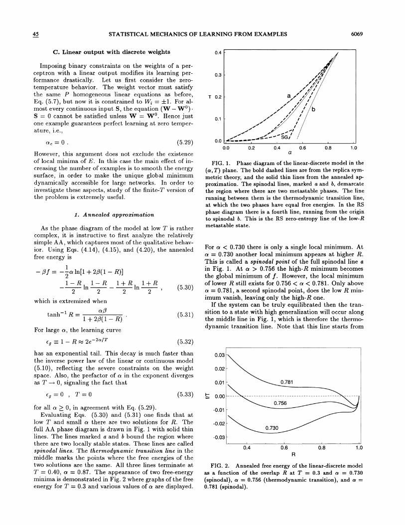
FIG. 1. Phase diagram of the linear-discrete model in the
(n, T) plane. The bold dashed lines are from the replica sym-
metric theory, and the solid thin lines from the annealed ap-proximation. The spinodal lines, marked a and b, demarcatethe region where there are two metastable phases. The linerunning between them is the thermodynamic transition line,at which the two phases have equal free energies. In the RSphase diagram there is a fourth line, running from the originto spinodal b. This is the RS zero-entropy line of the low-Rmetastable state.
For n & 0.730 there is only a single local minimum. Atn = 0.730 another local minimum appears at higher R.This is called a spinodal point of the full spinodal line ain Fig. 1. At n & 0.756 the high-R minimum becomesthe global minimum of f Howe. ver, the local minimumof lower R still exists for 0.756 & n & 0.781. Only aboven = 0.781, a second spinodal point, does the low R min-imum vanish, leaving only the high-R one.
If the system can be truly equilibrated then the tran-sition to a state with high generalization will occur alongthe middle line in Fig. 1, which is therefore the thermo-dynamic transition line. Note that this line starts from
0.03
0.02
0.01
~g——0, T=0 (5.33) 0.00
for all n ) 0, in agreement with Eq. (5.29).Evaluating Eqs. (5.30) and (5.31) one finds that at
low T and small n there are two solutions for R. Thefull AA phase diagram is drawn in Fig. 1 with solid thinlines. The lines marked a and b bound the region wherethere are two locally stable states. These lines are calledspinodal lines. The thermodynamic transition hne in themiddle marks the points where the free energies of thetwo solutions are the same. All three lines terminate atT = 0.40, n = 0.87. The appearance of two free-energyminima is demonstrated in Fig. 2 where graphs of the freeenergy for T = 0.3 and various values of n are displayed.
-0.01
-0.02
-0.03—I
0.4I
0.6R
I
0.8 1.0
FIG. 2. Annealed free energy of the linear-discrete modelas a function of the overlap R at T = 0.3 and o. = 0.730(spinodal), a = 0.756 (thermodynamic transition), and a =0.781 (spinodal).

6070 H. S. SEUNG, H. SOMPOLINSKY, AND N. TISHBY 45
the origin n = T = 0, implying that for any n as T ~ 0the equilibrium state is the high-R state. Since in thisstate R ~ 1 as T —+ 0 the equilibrium state at T ~ 0is always R = 1, in agreement with Eq. (5.29). However,the line approaches the origin as
n~Q. (5.34)
This implies that for a small number of examples even asmall noise in the dynamics will generate a transition tothe low-R state.
For training in large networks the most important tran-sition is, in general, not the thermodynamic one, butrather the spinodal line b. This is because starting frominitially random weights (R 0), the system convergesquickly to the nearest metastable state, which is the statewith low R as long as such a state exists. The timerequired to cross the free-energy barrier to the thermo-dynamic high-R phase is prohibitively large, scaling ast e~N+/ where 6f is the height of the free-energy bar-rier (per weight) between the two states. It is importantto note that, unlike the equilibrium transition line, thespinodal line terminates at T = 0 at a finite value of n,a = 0.556. This implies that in spite of Eq. (5.29), afinite value of n is required to learn in a finite time. Ac-cording to the AA the minimal value of n for learning atT = 0 in finite time, denoted by n„ is n, = 0.556.
the saddle-point equations for q and R, Eqs. (5.36) and(5.37), behave like
R —tanh R = tanh(nP),
q tanh R tanh (nP) .
(5.42)
(5.43)
n, =0,n, = 0.48,
(5.44)
(5.45)
respectively. The result n, = 0 implies that for any n )0, the training energy possesses a unique global minimumR = 1. However, the training energy may still possesslow-R metastable states. These states vanish above thespinodal point n, = 0.48.
Hence the generalization curve has the same exponentialtail ez 2e / as given by the AA in Eq. (5.32).
The RS phase diagram is drawn with bold dashed linesin Fig, 1. The similarity of the RS phase boundaries tothose of the AA (thin solid lines) is remarkable. Betweenthe spinodal lines marked a and b, there are two locallystable solutions of the saddle-point equations. The ther-modynamic transition line runs between the two spin-odals. The line running from the origin to spinodal b isthe RS zero entropy line of the low R metastable state.
At T = 0 the thermodynamic transition line and thespinodal line b intersect the n axis at
8. Replica symmetric theory
The replicated Hamiltonian G„, Eq. (4.27), which de-pends on the error function but not on the weight con-straints, remains the same as in Eq. (5.2). The resultingsaddle-point equations are
R = Dztanh qz+ R
q = Dztanh qz+ R
(5.36)
(5.37)
1+P(1 —q)' (5.38)
q —2R+ 1
[1+P(1 —~)1'For any fixed temperature, R ~ 1 and q ~ 1 as n ~ oo.To investigate this approach to the optimum, we notethat for large n
(5.39)
nP [2(1 —R) —(1 —q)], (5.40)R oP. (5.41)
Clearly there is a divergence of R, the strength of theordering term in the local field of Eq. (4.30). At thesame time, ~q/R ~ 0, so that the relative strength ofthe disordering term is going to zero. This means that
The replica symmetric free energy is given byEq. (4.25) where Gp, Eq. (4.26), is
1Gp ————(1 —q)q —RR+ Dz ln 2 cosh(+qz + R) .
2
(5.35)
8. Numerical simulations
We have used the Metropolis Monte Carlo algorithm tosimulate learning in the linear-discrete perceptron. Thisalgorithm is a standard technique for calculating ther-mal averages over Gibbs distributions [38]. The simu-lations were performed for multiple samples, i.e. , difFer-ent training sets drawn randomly from a common in-
put distribution. Here the inputs were chosen to beS, = +I at random, i.e. , S was drawn randomly fromthe vertices of the N-dimensional hypercube. This dis-crete input distribution allowed us to take advantage ofthe speedup ofFered by integer arithmetic, yet leads tothe same learning curves as the Gaussian input distribu-tion (4.3) in the thermodynamic limit (see Appendix C).The quenched average was performed over these samples,and error bars were calculated from the standard error ofmeasurement of the sample distribution. In the figuresof this paper, when a Monte Carlo data point lacks anerror bar, it means that the error bar would have beensmaller than the symbol used to draw that point. In gen-eral, fewer samples were required for larger N, becauseof self-averaging.
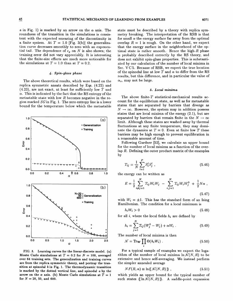
In Fig. 3 we present the numerical results as well as theRS theoretical predictions for the training and generaliza-tion errors as a function of n. The results of the RS the-ory are in very good quantitative agreement with MonteCarlo simulations of the model at least for T ) 0.2. AtT = 0.2 [Fig. 3(a)] the prominent feature is the rapidtransition to R 1 near n 0.65. This is in agreementwith the spinodal point n, = 0.66 for this temperature,which can be read from line b in Fig. 1. The locationof the thermodynamic transition is shown by a dottedvertical line, and the first spinodal (corresponding to line
45 STATISTICAL MECHANICS OF LEARNING FROM EXAMPLES 6071
g. Spin glass -phase
The above theoretical results, which were based on thereplica syrnrnetric ansatz described by Eqs. (4.22) and(4.23), are not exact, at least for sufficiently low T andn. This is indicated by the fact that the RS entropy of themetastable state with low R becomes negative in the re-gion marked SG in Fig. 1. The zero entropy line is a lowerbound for the temperature below which the metastable
1.0-
0.8-0 Generalization
o Training
0.6-
04
0.2-
a in Fig. 1) is marked by an arrow on the a axis. Theroundness of the transition in the simulations is consis-tent with the expected smearing of the discontinuity ina finite system. At T = 1.0 [Fig. 3(b)] the generaliza-tion curve decreases smoothly to zero with an exponen-tial tail. The dependence of ez on N is also shown; thetraining error did not vary appreciably. It is interestingthat the finite-size effects are much more noticeable forthe simulations at T = 1.0 than at T = 0.2.
state must be described by a theory with replica sym-metry breaking. The interpretation of the RSB is thatfor small o, the energy surface far away from the optimaloverlap R = 1 is rough. On the other hand, we expectthat the energy surface in the neighborhood of the op-timal state is rather smooth. Hence the high-R phaseis probably described correctly by the RS theory, anddoes not exhibit spin-glass properties. This is substanti-ated by our calculation of the number of local minima inSec. V C 5. Because of RSB, we expect the true locationof the spinodal line at low T and n to differ from the RSresults, but this difference, and in particular the value ofe„may not be large.
$. Local minima
The above finite-T statistical-mechanical results ac-count for the equilibrium state, as well as for metastablestates that are separated by barriers that diverge asN —+ oo. However, the system may in addition possessstates that are local minima of the energy (2.1), but areseparated by barriers that remain finite in the N -+ oolimit. Although these states are washed away by thermalfIuctuations at any finite temperature, they may domi-nate the dynamics at T = 0. Even at finite low T thesebarriers may be high enough to prevent equilibration ina reasonable amount of time.
Following Gardner [52], we calculate an upper boundfor the number of local minima as a function of the over-lap R. Defining the outer product matrix of the examplesby
P
0.0 -,
0.0 0.2
: O0 0 0 0 ~ O 0
0I
) o.e0.4 0.8 1.0 the energy can be written as
(5.46)
1.0-
0.8-
0.6-
N
) TqW W~ + Nn, —i,j=1
(5.47)
with W; = +1. This has the standard form of an IsingHamiltonian. The condition for a local minimum is
0.4-h;W; &0
for all i, where the local fields h; are defined by
(5.48)
0.2- h; = ) T;~ (W~ —W~) + rr W; . (5.49)
0.0 -,
0.0 0.5 1.0 1.5 2.0 2.5
The number of local minima is then
O(h;W;) . (5.50)
FIG. 3. Learning curves for the linear-discrete model. (a)Monte Carlo simulations at T = 0.2 for N = 100, averagedover 64 training sets. The generalization and training curvesare from the replica symmetric theory, and portray the tran-sition at spinodal 6 in Fig. 1. The thermodynamic transitionis marked by the dotted vertical line, and spinodal a by thearrow on the a axis. (b) Monte Carlo simulations at T = 1for N = 20, 50, and 600.
For a typical sample of examples we expect the loga-rithm of the number of local minima in'(N, R) to beextensive and hence self-averaging. We instead performthe simpler annealed average
NF(R, n) = ln((A/(N, R) )), (5.51)which yields an upper bound for the typical number ofsuch states ((ln Af(N, R) )). A saddle-point expansion
6072 H. S. SEUNG, H. SOMPOLINSKY, AND N. TISHBY 45
yields
F(R = l, n) = 0
and (for R ( 1)
ln H( y)—
1 —R 6 1+~
ln H(z) + —(z+ y)')2 2
n (z (1 —R)y2——~
—+ ln + ln22 (y1 —R 1 —R 1+R 1+R
ln ln2 2 2 2
Here we have defined
(5.52)
(5.53)
confirmed by numerical simulations of the model at T =0. We have found that the system converges rapidly toR = 1 from almost all initial conditions for
n&1.0. (5.55)
D. Boolean output with discrete weights
This Boolean-discrete model, first studied by Gardnerand Derrida [23], exhibits a first-order transition froma state of poor learning to a state of perfect learning[37, 53]. Unlike the linear-discrete perceptron discussedabove, this model's transition persists at all tempera-tures. The occurrence of this remarkable transition canbe understood using the high-temperature limit.
(5.54) The high-temperutere limit
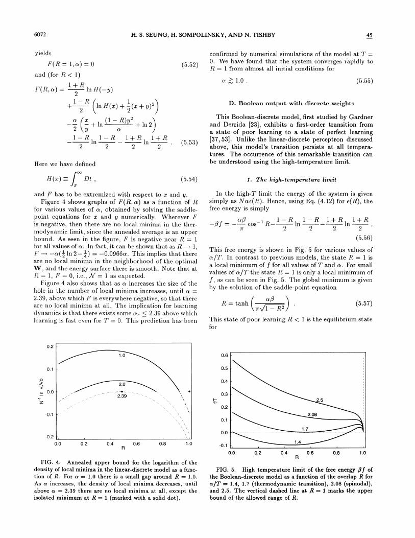
and F has to be extremized with respect to z and y.Figure 4 shows graphs of F(R, n) as a function of R
for various values of o. , obtained by solving the saddle-point equations for z and y numerically. Wherever I"is negative, then there are no local minima in the ther-modynamic limit, since the annealed average is an upperbound. As seen in the figure, F is negative near R = 1for all values of o. In fact, it can be shown that as R ~ 1,F ~ —n(z In 2 —
&) = —0.0966n. This implies that thereare no local minima in the neighborhood of the optimalW, and the energy surface there is smooth. Note that atR = 1, F = 0, i.e. ,
A' = 1 as expected.Figure 4 also shows that as o. increases the size of the
hole in the number of local minima increases, until o. =2.39, above which I" is everywhere negative, so that thereare no local minima at all. The implication for learningdynamics is that there exists some o., & 2.39 above whichlearning is fast even for T = O. This prediction has been
In the high-T limit the energy of the system is givensimply as Nnc(R). Hence, using Eq. (4.12) for c(R), thefree energy is simply
nP, 1 —R 1 —R 1+R 1+Rcos 'R— ln ln
2 2 2 2
(5.56)
R= tanhnP1 —R~
(5.57)
This state of poor learning R & 1 is the equilibrium statefor
This free energy is shown in Fig. 5 for various values ofn/T. In contrast to previous models, the state R = 1 isa local minimum of f for all values of T and n. For smallvalues of n/T the state R = 1 is only a local minimum off, as can be seen in Fig. 5. The global minimum is givenby the solution of the saddle-point equation
0.2—
0.6-
0.1 0.5—
c2.39
-0.1
0.2-
0.1
-0.2 —,
0.0I
0.2I
0.4I
0.6I
0.8 1.0
0.0—
-0.1
0.0 0.2 0.4 0.6R
0.8 1.0
FIG. 4. Annealed upper bound for the logarithm of thedensity of local minima in the linear-discrete model as a func-tion of R. For n = I.o there is a small gap around R = 1.0.As a increases, the density of local minima decreases, untilabove a = 2.39 there are no local minima at all, except theisolated minimum at R = 1 (marked with a solid dot).
FIG. 5. High temperature limit of the free energy Pf ofthe Boolean-discrete model as a function of the overlap R forn/T = 1.4, 1.7 (thermodynamic transition), 2.08 (spinodal),and 2.5. The vertical dashed line at R = 1 marks the upperbound of the allowed range of R.

STATISTICAL MECHANICS OF LEARNING FROM EXAMPLES 6073
T & 0.59A . (5.58) 2. Replica symmetric theory
In this regime the optimal state R = 1 is only metastable.If the initial network has R which is close to 1 the learningdynamics will converge fast to the state R = 1. Howeverstarting from a random initial weight vector R 0 thesystem will not converge to the optimal state.
For T/a & 0.59 the equilibrium state is R = 1, al-
though there is still a local minimum, i.e. , a solution ofEq. (5.57) with R & 1. Finally for
Because of the unusual features of the transition inthis model we will analyze the quenched theory in somedetail. We first study the replica symmetric theory andthen investigate the replica symmetry breaking in thissystem.
The RS free energy is given by combining Go of theperceptron with discrete weights, Eq. (5.35), with G„ fora Boolean output, Eq. (5.17), yielding
T & 0.48A, (5.59) 1—Pf = —-(1 —q)q —RR+ Dz ln 2 cosh(Qqz + R)2
there is no solution with R & 1 to Eq. (5.57). In thisregime (beyond the spinodal), starting from any initialcondition the system converges fast to the optimal state.
The collapse of the system to the energy ground stateat finite temperature is an unusual phenomenon. Theorigin of this behavior is the square-root singularity ofc(R) at R = 1. This singularity implies that a statecharacterized by bR = 1 —R « 1 has an energy which isproportional to R = Dz tanh qz+ R (5.67)
Dy Dtln e P+ (1 —e ~)H(u)0 —OO
(5.66)
where the function H(z) is as defined in (5.54). Thesaddle-point equations are
E oc N MSR . (5.60)q = Dztanh qz+ R (5.68)
SNGo(R) oc N(SR) ln (SR) . (5.61)
This big increase in energy cannot be offset by the gainin entropy, which is proportional to OO e-o2/2
R= Dtz gl —q (eP —1)-' + H(v)
' (5.69)
This effect can be nicely seen using the microcanonicaldescription. According to Eq. (2.27) above, a smoothlow-temperature limit exists provided that
Bs c)lim =oo.
&~&min(5.62)
On the other hand, Eq. (4.20) implies that in the presentcase
88(c) —~ln~, ~~0. (5.63)
Thus the rate of increase in entropy is too small to giverise to thermal fluctuations below some critical temper-ature.
It is instructive to apply the above argument to thecase of states that differ from the ground state by a flipof a single weight. According to Eq. (5.60) the energy ofsuch states is
2OO OO eq = Dy Dt
(1 —q) o K" —1) '+ ( )j' '
(5.70)
where u and v are given by Eqs. (5.18) and (5.'23) above.At T = 0, the equations simplify somewhat, since q =
R and q = R. For n less than
o, , = 1.245, (5.71)
there are two solutions, one with R = 1 (perfect gen-eralization), and one with R & 1 (poor generalization).The R & 1 saddle point has the lower free energy, andis therefore the equilibrium phase. Upon crossing thiscritical o. , the balance of free energy shifts, and thereis a first-order transition to the R = 1 state. Hence ato,, = 1.245 there is a discontinuity in the generalizationcurve, a sudden transition to perfect learning. However,the R & 1 state still remains as a metastable phase untilthe spinodal point
E oc V N, (5.64)o,, =1492. (5.72)
whereas the entropy associated with such an excitationis only
SNGo(R) oc ln N .
It should be emphasized, however, that examining thespectrum of the first excitations is not generally su%cientfor determining the thermodynamic behavior at any fi-nite T, where the relevant states are those with energyof order NT.
At any fixed T, there is the same sequence of thermo-dynamic transition followed by spinodal transition withincreasing a. The RS phase diagram is shown in Fig. 6.To the left of the dashed thermodynamic transition line,the state of poor generalization R & 1 is the equilibriumstate, and the state of perfect generalization R = 1 ismetastable. In the region between the dashed line andthe solid spinodal line, the situation reverses, with R = 1becoming the equilibrium state and R & 1 the metastablestate. To the right of the spinodal line, there is no low Rmetastable state.

6074 H. S. SEUNG, H. SOMPOLINSKY, AND N. TISHBY 45
1.0- (((~ ) )) . (5.73)
08 - PoThe parameter qo represents the average overlap betweena pair of two different states a and 6, i.e. ,
0.6- « = + (((~ )& ' (~b)T )) . (5.74)
0.4—
0.2-
When the n ~ Q limit is taken, the size rn of the step in
q(z) (see Appendix E) must be determined variationally,like qo and q~. Denoting the Gibbs probabilities of thediH'erent states by P, = exp( —PF, ), it can be shown [45]that
0.0 -,
1.0 1.5I
2.0a
I
2.5I
3.0
FIG. 6. RS and one-step RSB phase diagram for theBoolean-discrete model. To the left of the dashed thermody-namic transition line, the equilibrium state has R ( 1 (poorgeneralization), while the perfect generalization state (R = 1)is metastable. Between the dashed line and the solid spinodalline the R = 1 state is the equilibrium one, while the R ( 1state is metastable. To the right of the spinodal line, thereis no 8 ( 1 phase. In the region marked "SG," the one-stepRSB calculation predicts a metastable spin-glass state.
m=1— p2a (5.75)
Hence m is the probability of finding two copies of thesystem in two different states.
In the present model, a one-step RSB solution existsin the regime marked SG in Fig. 6, below the line Tz(n)This SG phase is special in that q~
—1, independent ofboth T and n. From Eq. (5.73) it follows that each ofthe different valleys is completely frozen, i.e. , there are nofluctuations in W within each valley. Indeed, the entropyof this phase is zero (to linear order in N) For fixed. n,the order parameter qo does not vary with temperaturewithin the SG phase; it is frozen at its value on the phaseboundary T&(n) The same. holds true for eq and R, i.e. ,
8. Replica symmetry breakingand metastable spin-glass phase
qo (T, n) = qo (T~ (n), n),e, (T, a) = e, (Tg(n), n),R(T, n) = R(Tg(n), n),
(5.76)
(5.77)(5.78)
The line Tz(n) in the T nplane, wh-ere the RS "poorgeneralization" state (R ( 1) has zero entropy, is the up-per border of the region marked SG in Fig. 6. It shouldbe noted that this line Tz(n) is to the right of the ther-modynamic transition line and coincides with it only atT = 0 (at a = 1.24). This implies that the RS theory isinvalid for this metastable phase only. To find the cor-rect metastable state (with poor generalization) at low Twe must search for saddle-point solutions to the replicatheory that break the replica symmetry.
To gain a better understanding of this metastablestate, we have studied a solution to the replica mean-field theory with a one-step replica symmetry breakingansatz. Our study is based on the work of Krauth andMezard [33] concerning the problem of loading randomdichotomies on a perceptron with discrete weights. Theformal derivation of the mean-field equations is presentedin Appendix E. Here we present the main results andtheir physical meaning.
In the one-step ansatz of replica symmetry breaking,the n x n order parameter matrix Q&„acquires two off-diagonal values qo and qq arranged in a block structure ofm x m submatrices (see Appendix E). This block struc-ture reflects the existence of many, almost degenerate,spin-glass (SG) states [45]. These states are valleys inthe free-energy surface that are separated by barriers thatdiverge with the system size [43]. The parameter qq rep-resents the overlap of each state with itself, i.e. , it is theorder parameter q, Eq. (2.56), measured within a singlevalley denoted a,
0.30-
0.25-
0.20-
0 0.15-UJ
0.10-
0.05—
0.00 —,
1.2 1.3I
1.4
Training
a
I
1.5I
1.6I
1.7
FIG. 7. Training and generalization errors of metastablespin glass phase in the Boolean-discrete model, according tothe one-step RSB ansatz. In this phase, the errors are inde-pendent of temperature, and are given by their RS values onthe zero-entropy line T~(a) of Fig. 6.
everywhere in the SG phase. The values of cq(n) andez(n) in this phase are shown in Fig. 7. The parameterm is linear in T, m = T/T~(n) Near t.he transitiontemperature T&, the degeneracy is very severe so thatm 1. At T = 0 the degeneracy is broken, and theGibbs weight concentrates in the SG metastable statewith minimal energy, resulting in rn = O.

45 STATISTICAL MECHANICS OF LEARNING FROM EXAMPLES 6075
A similar frozen SG phase exists in the perceptronmodel of Krauth and Mezard [33], and was first discov-ered by Derrida in the random-energy model [54]. How-ever, unlike these other examples, the SG phase in thepresent model is only a metastable phase, as evidencedby the nonzero e& in Fig. 7. Hence the one-step RSBtheory does not alter the RS prediction that the zerotemperature thermodynamic transition is at o = 1.245.However, it raises to
1.45-
1.40-
1.35-
o,, = 1.628 (5.79) 1.25-
the spinodal line for the vanishing of the metastable SGphase in Fig. 6.
g. Numerical simulations
1.20 -,
0.0I
0.02 0.041/N
I
0.06 0.08I
0.10
Figure 8 shows learning curves for Monte Carlo sim-ulations with N = 75, averaged over 32 samples. AtT = 1, there is quite a good fit if the transition is takento occur at the spinodal line. At lower temperatures, theMetropolis algorithm tends to become trapped in localminima, making equilibration dif6cult. Hence we cannotuse it to check the T = 0 predictions of the quenchedtheory.
The Metropolis algorithm produces a random walkthrough weight space that samples the Gibbs distribu-tion. For small system sizes, we do not have to samplethe weight space; we can explore it exhaustively. Gard-ner and Derrida [23] applied this idea to compute n, atT = 0. Starting with all 2N possible student vectors,an example is chosen at random, and all student vectorsthat "disagree" with the teacher are eliminated. Eventu-ally some number of examples P is reached such that theaddition of one more example produces perfect learning.Then n, (N) = P/N for this sample. The procedure isthen repeated with a different set of examples, so that o;,can be sample averaged.
FIG. g. Graph of n, vs 1/N at T = 0 for the Boolean-discrete model from exhaustive search. Each data point is theaverage of roughly 10 or 10 random samples of examples.The error bars are the standard error of measurement overthe sample distribution. A least-squares fit to a quadraticfunction yields the extrapolation n, (N = oo) = 1.30 + 0.03.The replica symmetric prediction a, = 1.24 is also marked.
We have extended the results of Gardner and Derridaup to the size N = 23. With the discrete inputs S; =+1, only odd N were used, so as to avoid the situationW S = 0. Figure 9 exhibits n, as a function of 1/N,with each data point an average of from 10s (large N) to10s (small N) samples. Fitting to a quadratic functionand extrapolating to N = oo yields the estimate n, =1.30+ 0.03, which is fairly close to the prediction 1.245of the quenched theory. It is possible that the quadraticfunction assumed here may be a poor approximation tothe true finite-size scaling. This would account for theremaining disagreement between the numerics and thetheory. See Ref. [55] for more simulations and an at temptat addressing the question of finite-size scaling.
0.5- VI. PERCEPTRON LEARNINGOF UNREALIZABLE RULES
04-
0.3-
0.2—
0.1
& Generalization
o Training
p
0
So far we have studied examples of perceptron learningof realizable rules. In this section we study three rulesthat are unrealizable because of architectural mismatch.In the first model, the student and teacher perceptronsare mismatched due to their different transfer functions.In the second and third models, the teacher's weight vec-tor is not included in the weight space of the student.
A. Linear-continuous perceptronwith unrealizable threshold
0.0 -,
0.0I
0.5I
1.0I
1.5 2.0I
2.5 3.0 3.5
FIG. 8. Learning curves for the Boolean-discrete model.Monte Carlo simulations at T = 1.0 and N = 75, averagedover 32 samples. The solid line and dashed lines are the RSgeneralization and training curves for the spinodal transition.The thermodynamic transition is marked by the dotted ver-tical line.
In this model, the perceptrons of the student andteacher both have linear outputs and continuous weights,as in the model of Sec. V A. However, in the present casethe transfer function of the teacher has a threshold, i.e. ,the rule is given by Eq. (4.5) with a transfer functiong(z) = gp(z), where
gp(z) = z y 0 .

6076 H. S. SEUNG, H. SOMPOLINSKY, AND N. TISHBY 45
g(z) = z . (6.2)
The realizable linear-continuous model of Sec. VA cor-responds to the case 8 = 0.
The average of the error function
1~(W; S) = [(W —Wo) S —V N8]2N (6 3)
The output of the trained network is given by Eq. (4.1)with
In the T ~ 0 limit there is a critical n below whichthe examples can be loaded with zero training error. Thisvalue is
2+ 02 —0+2+ 02
2(6.12)
For n & n„q is less than 1 and the values of the orderparameters are given by the saddle-point equations
(6.13)over the input distribution, Eq. (4.3), yields the general-ization error
n02g = n+
1 —n(6.14)
12e(W) = 1 —R+ —8
2 (6 4)
1 p02pf = p—fe=o ——
2~1 p(1 ), (6.6)
where fe 0 is the —RS free energy of the realizable case;see Eqs. (5.1) and (5.2). The saddle-point equations arethe same as (5.3)—(5.6), except that Eq. (5.6) for q mustbe modified to
2q —2R+ 1+ 0
[I+P(1 —q)]'(6 7)
For fixed temperature and n —+ oo, we find the asymp-totic learning curves
At R = 1, the generalization error takes on its minimumvalue e;„=82/2. Recall that according to Eq. (2.58),the average training and generalization errors both ap-proach cmj„as n ~ oo, at all T.
As in the linear-continuous model, the T = 0 behaviorcan be understood from geometric arguments. Weightvectors with zero training error must satisfy P linearequations
(W —W ) S' = MN0, t = 1. . . P (6.5)
and the spherical constraint W W = N. There existsan n, ( 1 such that for n & n„ these equations havesolutions. For n ) n„ the equations have no solution, sothat the training error rises from zero, and asymptoticallyapproaches E'~jn as n ~ oo.
The RS free energy is
In this regime the minimum of e& is highly degeneratewith an extensive zero-temperature entropy. Note thatfor any threshold 0, the critical n satisfies the boundsI/2&n, &1. Forn) o„q~1 asT~O, withP(1 —q) approaching a finite value. Thus at T = 0 theorder parameters are given above n, by
2Rs = (2+ n + 0')R' —n,
P(1 —q) = R(6.15)
(6.16)
The zero temperature n, of this and other unrealiz-able models is similar to the n, defined for the prob-lem of loading random patterns onto a network. In bothcases n, is the limit of storage capacity above which noweight vectors can achieve zero training error. This is incontrast to the n, that we defined for realizable models,above which there is exactly one weight vector which canachieve zero training error.
As in the zero-threshold linear-continuous model, weexpect that in this linear model the RS theory is exact forall T and n. Furthermore, the learning dynamics shouldbe quick, since there are no spurious local minima in thetraining energy.
In Sec. II D we noted that the AA may yield the wrongn —+ oo limit, for unrealizable, non-Boolean rules. Thepresent model is a simple example of this phenomenon.In the present case, G, Eq. (4.14), is
=1 P02G,„(R)= —in[1+ 2p(1 —R)] +—
(6.17)T+ 0'
ee——e~;„+ + O(n ),2n
T —0t: min+ + ( ).2n
(6.9) P f(R) = ——ln(l —R ) ——ln [1+2P(1 —R)]2 2
(6.8) The resulting annealed free energy, Eq. (4.13), is
To compare with the general results Eqs. (3.12) and(3.14) for smooth networks, we note that in the presentcase 0;e(W, S) = N i 0S, and 0;Bze(W— , S)N S,Sz, so that the matrices defined in Eqs. (3.4) and(3.5) are
2 1+ 2P(1 —R)(6.18)
In the n —+ oo limit R is determined by minimizing G „,yielding
U~=N 0 b~.
(6.10)
(6.11)
1, 0'(TR= 1 —i(02 —T), T & 02 & T+4
—1, T+4&0'.(6.19)
Hence the coeKcient N Tr VU in Eqs. (3.12) and(3.14) equals 02, in agreement with Eq. (6.8) above.
According to these results, when 0 ~ 4 and T = 0, theweight vector W approaches —W as n ~ oo.

45 STATISTICAL MECHANICS OF LEARNING FROM EXAMPLES 6077
1 pg(1 —R) 0
~~ 1+2P(1 —R)(6.20)
implying that the inputs are biased towards —0W . Itis important to note that the magnitude of the bias issmall —down by ~N from the magnitude of S. However,it is enough to push W towards —W, leading to overlapsas low as R = —1. Finally, note that in the realizable case0 = 0, the average of S is zero. However, even in thiscase the second moments of S are in general distorted,except when R = 1. This is consistent with the generalexpectation that the distortions of the input distribution,implied by the AA, are relatively small in realizable rules.But they vanish only in the limit of o. ~ oo.
B. Linear output with weight mismatch
To understand the origin of this gross failure of theannealed approximation we recall from Sec. II D that theannealed approximation can be viewed as the exact the-ory for a stochastic training dynamics in both weight andinput space, leading to the Gibbs distribution (2.43) inboth W and S space. The magnitude of the resultingdistortion in the posterior distribution of the inputs rel-ative to their a priori one determines the quality of theapproximation. In the present case we can obtain a mea-sure of this distortion by calculating the average of aninput vector, e.g. , (S~) „. In the a priori Gaussian dis-tribution of inputs (4.3), the average value of an input isof course zero. On the other hand, evaluating this aver-
age using the posterior Gibbs distribution (2.43), impliedby the AA, we find
~min: 1 —Roo: 0.202 (6.24)
Before we present the replica solution we note thatboth the high-T and the annealed approximations predictfor this model e&(n) —e,„ocn, n ~ oo. As we shallsee below, this is not the correct asymptotic behavior.
f. Bey/ica symmetric theory
R ~ q—2R+ I
(I- q)' ll+P(I-q))' '
nP(1 —q)1+P(1 —q)
'
q = Dztanh (+qz) .
(6.26)
(6.27)
(6.28)
To obtain the asymptotic form of the learning curves we
have expanded the solutions in powers of o. keeping Tfixed. We find
Here the replicated Hamiltonian G„ is that of the pre-vious linear models, Eq. (5.2). From Eq. (4.26) Go maybe calculated for the case of mismatched weight spaces.Making the change of variables q+ R ~ q, and theneliminating R altogether, one obtains the free energy
1 1 R2Pf—= ——(1 —q)q —— + Dz ln 2 cosh(Qqz)
2 2 1 —q
——In[1+ P(1 —q)] ——Q n P(q —2R+ 1)(6.25)
2 2 1+P(1 —q)
The saddle-point equations are
In this model, the unrealizability is due to a mismatchin weight space between teacher and student. We as-sume that the weights of the teacher network W arereal valued whereas the trained network is restricted toW; = +1. For simplicity we consider here the case wherethe individual teacher weights W; are drawn from a con-tinuous Gaussian distribution P(W; ),
&min R~&g = &min+
A'
3 3 5+R ——————+4R2 7r3 7r
~' ( 6R+—l
T —l
—+ 0(n ), (6.29)24 ( z2 ) n2
P(Wo) (2 )-1/2 —(1/2)(w, ) (6.21)
~t —&min&min R~
W;* = sgn(W; ), (6.22)
which corresponds to the maximal overlap
R = —) lw'l
dW PW W = 27r. (6.23)
As in the previous linear perceptron models the errorfunction is given by Eq. (4.9), and the generalization er-ror for a given network by Eq. (4.10). In the presentmodel the optimal weights for the restricted architectureof the trained network are
+Rl
—+ ——R + T'l
—+0(n—-s) .k2 z 24 ) nz
(6.30)
Thus for any fixed T the leading behavior of the errors isan o. power law. This power law is not a consequenceof the general results (3.12) and (3.14), since the presentnetwork is not smooth. Note that in the high-T limit,only the term T a survives. Thus for this unrealizablerule the behavior predicted by the high-T limit (as wellas by the annealed approximation) does not reflect thecorrect behavior at large 0 for any fixed T.
In the T ~ 0 limit with 1 —q finite the saddle-point
equations reduce toThe second equality holds in the thermodynamic limit.The minimal generalization error, achieved in the limitA ~oo) ls
R=0. ,
q(1 —q) = —n2+ n(1+ q),(6.31)(6.32)

6078 H. S. SEUNG, H. SOMPOLINSKY, AND N. TISHBY 45
1 —q = Dz sech qz (6.33)0.25-
Criticality is reached when q ~ oo, and 1 —q
—+ 0, whichhappens at
0.20-
( 2) i/2n, = 1 —
i1 ——
i
= 0.397 .z') (6.34)
0.15—
0.10-Above n„ the limit P ~ oo must be taken with P(1 —q)constant, yielding 0.05-
0 = 2R —(2+ n)R + (6.35)
(6.36)
0.00 -,
0.0 0.5I
10 50
At n„p(1 —q) diverges, indicating that the finite 1 —q
solution takes over.
2. Optimal temperature
FIG. 10. The RS zero-entropy line for the linear-mismatched model, which is a lower bound for the temper-ature at which RSB occurs. The line approaches the limitT = 0.242 (dashed line) as n ~ oo.
We define the optimal temperature T &t, (n) as the tem-perature that minimizes es(T, n). For our models of real-izable rules, the optimal generalization error was at T = 0for all values of n. But in general, T pt, may be greaterthan zero, although the convexity of the free energy guar-antees that the training error is a nondecreasing functionof T. This is the case in the present model, as can beseen from Eq. (6.29), which implies that
(6.37)
8. Replica symmetry breaking
The above RS theory is not exact at low T First, .the prediction of a finite value of o., is probably incor-rect. As in the corresponding realizable discrete modelof Sec. V 8, we expect that
n, =o, (6.38)
i.e. , there is no vector of discrete weights that satisfies or-der N real, random linear equations. Second, the entropyof the RS solution becomes negative at low T, as shownin Fig. 10. The asymptotic form of the zero-entropy linecan be calculated by expanding the entropy in powers of
as o. ~ oo. Note, however, that the leading term ofEq. (6.29) is independent of T, implying that in thepresent model the effect on es of optimizing with respectto T is relatively small.
temperature gives a lower bound on the temperature atwhich replica symmetry is broken. Below this tempera-ture, a spin-glass phase with replica symmetry breakingoccurs. As T ~ 0, the zero-entropy line approaches theorigin, i.e. , the RS entropy is negative for all n at T = 0.This means that the RS solution is incorrect at T = 0 forany n, and in particular that the RS prediction (6.34) forn, is incorrect, which is consistent with our prediction,Eq. (6.38).
Below T = 0.242, the system never escapes from thespin-glass phase even as n ~ oo (see Fig. 10). Note,however, that the entropy (6.39) approaches zero frombelow. This suggests that the eKects of RSB become lesssevere as o. ~ oo.
g. Numerical simulations
Figure 11 exhibits Monte Carlo simulations at T = 0.5and 0.1 with 1V = 100 and 64 samples. Even at T = 0.1[Fig. 11(b)j the fit to the RS theory is very good, even
though for a ) 0.76 the curves are in the RSB region.This suggests that the eKects of RSB in this system areweak. The RS T = 0 learning curves are also plotted forcomparison. Note that above n ) 0.6, the generalizat, ionerror for T = 0.1 is less than that at T = 0. At leastin this range, we may thus conclude that the optimalgeneralization temperature T pt- ) 0, assuming that theRS theory is a good approximation for the true behaviorin the RSB region.
(6.39)
The s = 0 temperature approaches the finite limit
3RT, ,(~) , = 0.242 (6.40)
as n ~ oo. The full line is drawn in Fig. 10 for all o.. This
C. Boolean output with weight mismatch
As in the previous model, the teacher weights are againdrawn from a continuous Gaussian distribution, whereasthe student weights are constrained to +1. However, herewe consider the case where the perceptron transfer func-tions of both the teacher and the student are Boolean.The maximal overlap is still R = g2/s, but the opti-mal generalization error is now

STATISTICAL MECHANICS OF LEARNING FROM EXAMPLES 6079
1;„=—cos R = 0.206 .7r
(6.41)where the function H(z) is as defined in (5.54) above.The saddle-point equations are
As in the previous model, both the high-T and the an-nealed approximations predict cs(n) —e~;„ocn, n ~oo. Vk shall see below that the true asymptotics arequite de'erent.
f. Replicu symmetric theory
For this model, Go is the same as that of the previoussection, and G„ is that of the previous Boolean models
Kq. (5.17). Hence the RS free energy is given by
1 . 1 R2Pf—= —-(1 —q)q —— + Dz ln 2 cosh(+jz)
2 2 1 —q
+2n Dy Dt ln [e ~ + (1 —e ~)H(u)0 —OO
(6.42)
1.0-
R oo —e /2Dt
+1 —qz. (e& —1)—'+ H(v)
' (6.43)
OO OO —tL2
e
t -~r 'f. "f= 'r ~- ~- + (.)i(6.44)
q = Dz tanh qz (6.45)
The quantities u and U are given by Eqs. (5.18) and (5.23)above.
The large-n limit of the RS theory is derived by ex-
pansion in 1/~n keeping P fixed,
1 z i&4 I(P) 1cs —~,„+ ——1 ( + 0(n '),
ps~' n
(6.46)
0.8-ion
where we have defined the integral
0UJ
0.6-
0.4-As P ~ oo, I(P) (2P)si z/3, so that
(6.47)
0.2 - ~p-a--o~D-D- D 0~a~ 0 4 ~a~ 0 0 0 ~
~/4 1~s(T = O, n) = c;„+-Q2/7r ——1 +0(n ') .
3 2 n
0.0 -,
0.0
1.0-
0.8-
I
0.5 1.0 1.5 2.0 2.5
(b)
(6.48)
Thus for any fixed temperature, the RS generalizationcurve possesses a 1/~n tail.
At T = 0, one solution of the RS equations is obtainedby taking the limit P ~ oo with 1—q finite. This solutionceases to exist when q ~ 1, which happens at the point
0.6-or
Rc
1 —R2Qc 2= —' =cot-7r O;c
(6.49)
UJ
0.4- n, = 1.99, R, = 0.534 . (6.50)
0.2
a p p p p p p p p
Above n„ the limit T -+ 0 must be taken with P(1 —q)finite, yielding
0.00.0 0.5 1.0
I
1.5I
2.0 2.5
—p(s —q)/(s —a') (6.51)
FIG. 11. Learning curves for the linear-mismatchedmodel. (a) Monte Carlo simulations at T = 0.5 with N = 100and 64 samples, with lines from RS theory. The dotted hor-izontal line is the asymptotic error c „. (b) Simulations atT = 0.1. Note that the RS curves (solid lines) fit the dataeven beyond the zero-entropy point a = 0.76, where thereis RSB. The dashed line is the T = 0 RS curve, shown forcomparison.
R~ —Qo Q~ ~20
(6.52)
The RS theory predicts that the optimal tempera-ture for generalization T &,(n) is nonzero for n above
ath = 1.27. The shape of T»t(a) for large n can be de-
rived using the high-temperature expansion of Appendix

6080 H. S. SEUNG, H. SOMPOLINSKY, AND N. TISHBY
F. The dominant terms are which leads to the power law
T pt; 0 239 ct' (6.54)
However, as we will see below, this RS optimal temper-ature lies below the zero temperature line, i.e. , in theregime where the RS solution is unstable.
2. Spin-glass phase
The RS entropy vanishes on the line shown in Fig. 12.Here again the 8 = 0 line provides a lower bound forthe spin-glass transition temperature. Comparing withFig. 10 two differences should be noted. First, the lineintersects the a axis at a finite value, at
o., = 1.106 . (6.55)
1 vr i~4 1 i/2 T&y: &mjn+ —1 T 0'+—
(6.53)
The I/~n term comes from expanding the coefficient ofthe quenched result (6.46) in P. Thus it represents theresult of first taking the T/o. ~ 0 limit and then theP ~ 0 limit. The I/n~ term is just the leading termfrom the high-T limit, which amounts to taking first theP ~ 0 limit and then the T/o. ~ 0 limit. The optimal Tat large a is obtained by minimizing with respect to T,yielding
0.315Q', 0! ~ oo . (6.57)
Eg(T, Q') —t~in ~ 0.185 o (6.58)
which is independent of T. This power-law decrease isfaster than the RS prediction I/~n, Eq. (6.48).
Equation (6.56) also reveals that at fixed T, the RS en-tropy goes to —oo as o, ~ oo, indicating that replicasymmetry is violated more and more severely.
Like the realizable Boolean model with discreteweights, this model possesses a frozen one-step RSB so-lution (see Appendix E). However, in contrast to theBoolean or discrete model, this one-step solution is theequilibrium, not the metastable phase, and exists for ar-bitrarily high n. According to this RSB solution there isspin-glass phase everywhere below the s = 0 line. Thetraining and generalization errors in the SG phase aregiven by their values on the phase boundary Tz ——T,—oat the same a [see Eq. (5.76)j. This is shown in the plotof es in Fig. 13. Since T~(n) is above the RS T ~i(o),there is no minimum in cz(T) for any n. Instead there isa whole regime of temperatures where e& does not changewith T, implying that optimal generalization can be ob-tained anywhere on or below the zero entropy line,
For any fixed T, the n ~ oo limit enters the RSBregime. Hence the large o, limit of E'g for any fixed T isgiven by substituting Eq. (6.57) in Eq. (6.53), yielding
Second, T,—ii(o. ) diverges with n. The asymptotic be-havior can be calculated using a double expansion in thevariables P and T/n In Appen. dix F, we discuss the ex-pansion, and how to locate the dominant; terms throughpower counting. They are
i/4 1 ~2 ~ 1/2 T8= ————1 — 0,' T+ ———14x 2 T 6 2
(6.56)
8. Numerical simulations
Figure 14 shows Monte Carlo simulations at T = 0.5and 1.0 with N = 75, averaged over 64 samples. Be-low T = 1 the training curve is significantly differentfrom the RS result. These deviations for T = 0.5 aresignificantly larger than those observed for the linear-
0.36-
0.34-
0.32-
0.30-
0.5— 0.28—
0.1
0.26 -,I
0.1
I
0.5
0.050.5
I
5a
10 50
FIG. 12. RS zero-entropy line for the Boolean-mis-matched model. The line intersects the a axis at the finitevalue a = 1.106.
FIG. 13. Generalization error for fixed a = 1.2, 1.6,2.0, 2.4, 2.8, and 3.2 as a function of T for the Boolean-mismatched model. Each curve is a combination of the one-step RSB solution below Ts(a) (marked with a dot on eachcurve) and the RS solution above. The light dotted lines arethe continuation of the RS curves below Ts(a). Note that theminimum of each of the RS curves is below Ts(a)

45 STATISTICAL MECHANICS OF LEARNING FROM EXAMPLES 6081
0.5-
0.4-
0.3-
0.2-
0.1-
0.0
dBi
O
(a)& Generalization
o Training
0 A
9 P o o a a. FCl ~~4QQgOoea e a a a e a a a a ~ '
I
10
in certain circumstances to train the system at finite Tbecause convergence times may be prohibitively long atT = 0. This is particularly true for highly nonlinearmodels, such as the Boolean perceptron with discreteweights. Although the critical number of examples perweight n, (T) increases with T in this model, we havefound in our simulations that the time it takes to con-verge to the optimal state in this model, increases dra-matically as T is lowered. It should be stressed howeverthat we have used only a simple Monte Carlo algorithm.Recently several heuristic training algorithms for percep-trons with binary weights have been proposed [34, 56]. Itwould be interesting to study their dynamic and gener-alization properties.
0.5
0.4o Generalization
o Training
0.3o o 0 0 a n
0.2-
0.10 0
0 00
e s o.
0 .0, .0. -O-p-p---p 0 0 Po~0~ir
0.0 -,I
10
FIG. 14. Learning curves for the Boolean-mismatchedmodel. (a) Simulations at T = 1.0 with N = 100 and 32samples. Each learning curve is a combination of the RS so-lution below the zero-entropy point a = 6.4 and the one-stepRSB solution above. The light dotted lines are the contin-uation of the RS curves above n = 6.4. (b) Simulations at7 = 0.5.
mismatched model, indicating the importance of RSB forthis model. The RSB solution fits fairly well at large o, ,
but in the vicinity of the transition, there are still somedeviations between the theory and simulations. Thesedeviations may be the result of difficulties in equilibrat-ing the system near the transition.
VII. DISCUSSION
A. Learning at Bnite temperature
In this paper we have studied the process of learningfrom examples with a stochastic training dynamics. Thelevel of noise in the dynamics is denoted by the tem-perature T. One of the most important results of ouranalysis is that learning at finite temperature is possi-ble, and sometimes advantageous. For any finite T, asthe number of examples increases, the network weightsapproach their optimal values, namely the values thatminimize the generalization error. Thus even when thegeneralization error increases with T it may be profitable
B. The high-temperatureand annealed approximations
%e have presented two approximate theoretical ap-proaches to the problem of learning from examples inlayered networks. The first approximation replaces thetraining energy by the number of examples times the gen-eralization error, and becomes exact in the limit of learn-ing with high thermal noise level. The dependence on Tand o; is only through the effective temperature T/nEven in this simple approximation, perceptron modelsexhibit a rich spectrum of generalization behaviors.
The second approximation, the annealed approxima-tion, reduces to the proper high-T limit, but deviatesfrom it significantly at finite o, and T, where the behav-ior is no longer a function of only the ratio of the twoparameters.
In all four realizable perceptron rules studied here,these approximations have predicted correctly the shapesof the learning curves at finite T and large o, . Further-more, the AA has yielded interesting results at finite Tand o, that are qualitatively correct. For instance, thefirst-order transitions predicted by the AA for the per-ceptrons with discrete weights are clearly observed in thesimulations, Figs. 3 and 8, and are in agreement with thefull quenched theory.
On the basis of our general arguments in Secs. II andIII, we expect that these approximations will also hold forrealizable rules in the more complex cases of multilayernetworks. This is borne out in recent, studies of tw~layernetworks of local feature detectors [35], and other mul-tilayer systems [36]. Thus these approximations providepowerful theoretical tools for the study of learning fromexamples, at least for realizable rules.
Our treatment should be contrasted with the di%cultproblems of the capacity of single- and multilayer net-works [57—59]. The capacity problems usually deal withloading random sets of data. In this case the systemis highly frustrated and one has to employ the complexmethods of spin-glass theory, such as replica symmetrybreaking [33, 60]. In the learning problems of the presentwork, the training set consists of very structured data,generated by a well-defined rule. The underlying struc-ture is represented in our formulation by the general-ization function e(VV), Eq. (2.4), which dominates the

6082 H. S. SEUNG, H. SOMPOLINSKY, AND N. TISHBY 45
behavior of the system at least when the number of ex-amples is large. This function would be completely flat,and therefore meaningless, in the case of random trainingsets.
In fact, the high-T limit ignores completely the fluc-tuations due to finite sampling of the rule. It is thususeful in studying how learning is affected by the na-ture of the target rule [e.g. , through the function c(W)]as well as by the network architecture [e.g. , the entropys(e), Eq. (2.26)]. As has been explained in Sec. III theAA does take into account the effect of randomness in-duced by the examples, though only approximately. Thereasonable results generated by the AA even at finite nand T imply that this randomness may not have majoreffects (e.g. , frustration and other spin-glass phenomena),at least in models where the chosen architecture is com-patible with the rule to be learned. This may explainwhy, in many applications of supervised learning, simplelocal gradient algorithms seem to yield good results.
It should be emphasized that the above approxima-tions may be useful not only for studying specific "toy"models, but also in generating general approximate pre-dictions that could perhaps be useful in applied researchon neural networks. An example is Eq. (2.40), which pro-vides a way of estimating the generalization error fromthe observed training error for a multilayer network wit;h
a Boolean output.
C. Inverse power law for smooth networks
The most important general result is the inverse powerlaw for the asymptotic behavior of both the generaliza-tion and training errors, Eqs. (3.12) and (3.14) of Sec. III.These results also provide a simple relationship betweenthe two errors, namely Eq. (3.15). This power law is
consistent with the general bound obtained within PAClearning theory. However, our theory is not distribution-free and holds only for smooth networks. On the otherhand, it holds for general unrealizable rules, whereas thePAC bounds are essentially for realizable rules.
The results regarding smooth networks were derivedusing a perturbative approach, i.e. , assuming that essen-tially all the components of W deviate only slightly fromW' for sufficiently large n. Of course in reality therecan also be contributions coming from W far away fromW*, leading to nonperturbative terms to ez. However, we
expect that for su%ciently large o. the nonperturbativeterms will be negligible (e.g. , exponentially dependent on
n) relative to the power-law contribution of the smoothfluctuations. On the other hand, these localized non-
perturbative errors may be important for the dynamicsof the training, since their relaxation may be extremelyslow compared with the continuous fluctuations.
In nonsmooth networks the generalization performancedepends on the nature of the task as well as the networkarchitecture, as the results of Secs. V and VI demon-strate. These results also indicate that there is a qual-itative difference between the learning of realizable andunrealizable rules, as discussed below.
D. Learning, realizable rules
The results of the specific models studied here indicatethat the shapes of learning curves may be very differentfrom the PAC learning bound of an inverse power law.The shape of the generalization curve depends stronglyon the degree of constraint imposed on the network space.In the case of a linear output, the imposition of binaryconstraints changes a T/n tail [Eq. (5.10)] into an expo-nential exp( —2n/T) [Eq. (5.32)]. In addition, at low Tthere is a discontinuous transition at finite o, from poorto good generalization; see Figs. 1 and 3. The superiorgeneralization ability of the constrained network is notsurprising. Since the target rule itself was assumed to berealizable in the constrained architecture, imposing theconstraints is essentially using prior knowledge (or as-
sumptions) of the nature of the rule to restrict the spaceof possible networks.
The most dramatic effect of constraining the network isfound for the conventional perceptron rule, i.e. , one witha Boolean output. In the unconstrained network the gen-eralization error again behaves as an inverse power law
[this time even at T = 0, Eq. (5.28)]. On the other hand,in the case of binary weights there is a discontinuous tran-sition at a critical a from poor to perfect learning (seeFig. 6). This transition is unique in that it exists evenin learning at high temperatures. The collapse of a ther-modynamic system at finite T to its ground state abovesome n, stems from the singular spectrum of excitationsabove this state, as discussed in Sec. V D.
In all the realizable models studied in this work, thequenched RS behavior at finite T is qualitatively similarto that given by the AA. Furthermore, the asymptoticshapes of the RS learning curves in the different mod-els agree with those of the AA. This suggests that forrealizable rules the effect of disorder is minor for large n.
The main qualitatively different result of the quenchedtheory is the appearance of spin-glass phases, as shown in
Figs. 1 and 6. These phases result from the randomnessand frustration associated with optimizing for a particu-lar realization of examples, and cannot be predicted bythe high-T or the annealed approximations. Two specialfeatures distinguish the SG phases of realizable models.First, it exists only at low T and in restricted regime of n,typically o. 1. Second, it is only metast;able, i.e. , its freeenergy (as well as training energy) is higher than that ofthe optimal state, which is therefore the true equilibriumstate in that regime of o.
The absence of SG phases at large n indicates thatas o, increases, the relative scale of fluctuations in thetraining energy becomes smaller, i.e. , the training en-
ergy surface get, s smoother as the number of examplesincreases. This is indeed demonstrated by the analyticalbounds of Sec. V B on the number of local minima for thelinear perceptron with discrete weights (Fig. 4). Thesebounds exhibit two important, and possibly general, fea-tures. First, the energy surface in the neighborhood ofthe optimal state R = 1 is smooth. Second, the numberof local minima is exponentially large for small e, butdecreases monotonically with a. In the linear-discretemodel there are no local minima above a critical value of

45 STATISTICAL MECHANICS OF LEARNING FROM EXAMPLES 6083
E. Classification of learning curvesfor realizable rules
The discontinuous behavior of the Boolean percep-tron with discrete weights calls for an understanding ofthe general conditions which determine whether a givenlearning task will be achieved gradually or not. Insightinto this question is provided by the high-T limit ofSec. II C. According to Eqs. (2.25)—(2.27), a system canbe classified according to the behavior of its entropy s(c).Recall that e '~'~ is defined as the number of networksthat yield a given generalization error e. The generalform of s(e) for small e is expected to be
s(c) ocr in~, a~0. (7.2)
For a smooth weight space we expect s to diverge log-arithmically to —oo, i.e. , z = 0. This naturally leads,via Eq. (2.27), to the inverse power law. For a discreteweight space, we expect the entropy to approach a finitevalue, i.e., z & 0. When 0 & z & 1 the generalizationcurve obeys a nontrivial power law
as=(nP) '~~' ~, nP~oo, 0(z(1. (73)up to logarithmic corrections. When z = 1 this law turnsinto an exponential,
ines oc —np, np ~ oo, (7.4)
An example of this case is the perceptron with discreteweights and linear output; see Eq. (5.32). When z &1, Os/Be remains finite at small e, so there must be adiscontinuous transition at some (nP), to es = 0,
cs = 0, aP & (nP)„z & 1 . (7 5)
The Boolean perceptron with discrete weights is an ex-ample of an entropy with z = 2; see Eqs. (5.6'2) and(5.63).
In our perceptron models, nontrivial shapes of learningcurves resulted only when the weights were constrainedto discrete values. In contrast, for multilayer networks weexpect that the exponent z in Eq. (7.2) may be nontrivialeven when the weights are allowed to vary continuously,possibly leading to Eq. (7.4) or (7.5). This will occur, forexample, if the optimal solution involves discrete internalrepresentations of the hidden neurons, as demonstrated
a. Fontanari and Koberle [61] have studied numericallythe local minima of the Boolean-discrete model for smallsystem sizes. The number of local minima was found toscale exponentially with N and to decrease monotonicallywith o, . No critical value of n for the disappearance oflocal minima in the Boolean model was found. However,a definitive conclusion would require the investigation oflarger sizes.
Finally, in all our realizable models the generalizationerror decreases monotonically with T, so that the optimaltemperature for learning is
Tops = o. (7 1)
Of course this refers to the equilibrium properties,whereas from dynamic point of view the optimal tem-peratures may be finite even in realizable rules, as hasbeen pointed out above.
in the two-layer model network for the contiguity problem[351.
The above classification requires knowledge of the be-havior of s(c) near e = 0. In general, evaluating s may bediKcult even in relatively simple models, since the pri-mary interest is its behavior in the limit N ~ oo. Forthis reason, the simple existence of a gap in the spec-trum of e is an insufIicient basis for classification. At thevery least, the scaling of the gap with N must be deter-mined (see Sec. IV F). Finally, it should be stressed thatthe classification of the asymptotic shapes of the learn-ing curves according to the properties of s(e) has beenjustified so far only in the high-T limit. It may be, how-
ever, that in many classes of realizable rules these resultsapply also to finite T or even T = 0. If this is true thenour results may provide useful hints for understanding oreven predicting the behavior of some real-world learningproblems.
F. Unrealizable rules
&s(~) &) &min ~ u' -a/5 (7.7)
An n i~z tail in es has also been found in Boolean Per-ceptrons with continuous weights where the rule is unre-alizable due to corruption of the examples by noise [24]or due to the random nature of the rule itself [22].
The RS theory of perceptrons with unrealizable rulespredicts that, for su%ciently large a, e& is nonmonotonicwith T, but possesses a nonzero optimal temperature.Similar results have been obtained in [22, 24]. In the caseof a Boolean perceptron with weight mismatch, wherethe corrections to RS theory could be calculated, it hasbeen found that rather than having a minimum at finiteT, e& is independent of T at low T; see Fig. 13. Whethercorrection to the RS theory will modify substantially theconclusions regarding T &t of the RS theory in the othermodels remains to be studied.
Another feature of unrealizable rules is the prevalence
For unrealizable rules the optimal weight vector W'is reached only in the limit n ~ oo. This is true at alltemperatures. As T ~ 0 the generic shape of the learn-ing curves is roughly that shown in Fig. 11(b). Thereis a critical value o., which marks the loading capacity,i.e. , the point below which the examples are memorizedperfectly. Above o., the training error increases, and ap-proaches the same limit as the generalization error, i.e.,
approaches e;„ from below as n ~ oo. Also, in someunrealizable models (not encountered in this work, butsee Refs. [22, 24]) there is a local maximum in es near n, .
One of the important results of our study is that for un-
realizable rules the learning curves are substantially dif-ferent from the high-T and AA predictions at any fixed T.For example, for the models with weight mismatch, theseapproximations predict n z tails for fixed T, whereas theRS theory yields [see Eqs. (6.29)]
~s(T, o.) —c;„-n
for the case of a linear output, . In the Boolean outputcase the full spin-glass theory predicts

6084 H. S. SEUNG, H. SOMPOLINSKY, AND N. TISHBY 45
of spin-glass phases even at large o, . In the present workwe have evaluated the T at which the entropy vanishes.This provides a lower bound for the onset of the spin-glassphase. Here again the linear and Boolean perceptronsdiH'er. In the linear case this temperature levels oA' at afinite value as e increases, as shown in Fig. 10. In theBoolean case it grows with the same power law as T pt,
.
see Eq. (6.57) and Fig. 12. These results suggest thatspin-glass eHects are strong in unrealizable cases.
The fact that the spin-glass phase exists also for large o.
suggests that the fluctuations in the training energy donot necessarily shrink as o, increases. Nevertheless, webelieve that their reLative scale does indeed vanish. Thisis because the energy itself grows linearly with o. . Thisconjecture is supported by the observation that the tem-perature that marks the onset of spin-glass phenomenagrows only sublinearly with n [see Eq. (6.57)]. The effectof increasing the number of examples on the roughness ofthe training energy surface (particularly in unrealizablerules) is an important issue which deserves further study.
APPENDIX A: TRAINING-GENERALIZATIONINEQUALITY
Let Ep denote the average value of the training energyPE(W), as in Eq. (2.18) and bE the difference E —Ep.Define the function
dp(W)e ~ ' ~ bE
dp(W)e-~~ -~~~(A1)
dp(W)e ~ 'bE
dp(W)e(A2)
This can be interpreted as the energy of a system attemperature I/P with Hamiltonian bE and measuredp(W)e ~+'. By the convexity of the free energy, theenergy is a decreasing function of P. Hence 6 is boundedabove,
G. Uniqueness of the optimal solution
Throughout this paper we have assumed that the opti-mal network weights, i.e. , the components of the weightvector W* that globally minimizes the generalizationfunction e(W), are unique. If they are nonunique, weassume that the degenerate global minima are at leastwidely separated in network space, forming a discreteset. This is related to our assumption that the trainingdynamics searches for the values of the network weightswithin a well-defined architecture. Under these condi-tions it is reasonable to expect that the optimal solutionis generally unique up to obvious symmetries. For in-stance, in multilayer networks the solution may be uniqueonly up to permutation of the hidden neurons [62]. Othersymmetries may result from the nature of the rule itself.An example is the up-down degeneracy of the optimalsolution of the two layer network of edge detectors inRef. [35). This uniqueness does not hold if the architec-ture of the network, e.g. , the number of neurons or thenumber of layers, is allowed to vary significantly. Theimportant issue of learning under these circumstances isplanned to be discussed elsewhere.
e((T, cr) ( ~g(T, n),which was stated without proof in Eq. (2.20).
(A4)
AP PEND IX B: HIGH- TEMP ERATU REEXPANSION
In this appendix, we show using a cumulant expansionthat the free energy (2.13) can be written as a powerseries in P, with coefficients that are functions of nP. Thezeroth-order term of this series is the high-temperaturelimit discussed in Sec. II C.
The first step is to separate the energy into randomand nonrandom parts. The nonrandom part is
Ep = (( E)) = Pe(W) = Nne(W),
and the random part is
(B1)
We now take the quenched average of both sides. Inthe integrals, the average can be applied directly to bE,since Ep is independent of the quenched disorder. But(( bE)) = 0, so the right-hand side vanishes, and we have
(A3)
In particular, for 7 = P, ((4)) = P(c, —cz), so that we
finally obtain
ACKNOWLEDGMENTSP
bE = E —Ep ——) bc„, (B2)
We would like to thank E. Baum, D. Hansel, D. Haus-sler, and D. Huse for helpful discussions. We are gratefulto G. Gyorgyi for his comments on an earlier version ofthe manuscript and for drawing our attention to the RSBphase in the Boolean model with mismatched weights.We also thank the Aspen Center for Physics for host-ing a Workshop on Neural Networks where part of thisresearch was conducted. H. S. S. acknowledges supportfrom Harvard University.
where
b~„= c(W; S")—e(W).
We now treat bE as a perturbation to the "free Hamil-tonian" Ep. The partition function takes the form
Here ()p denotes the average with respect to the distri-
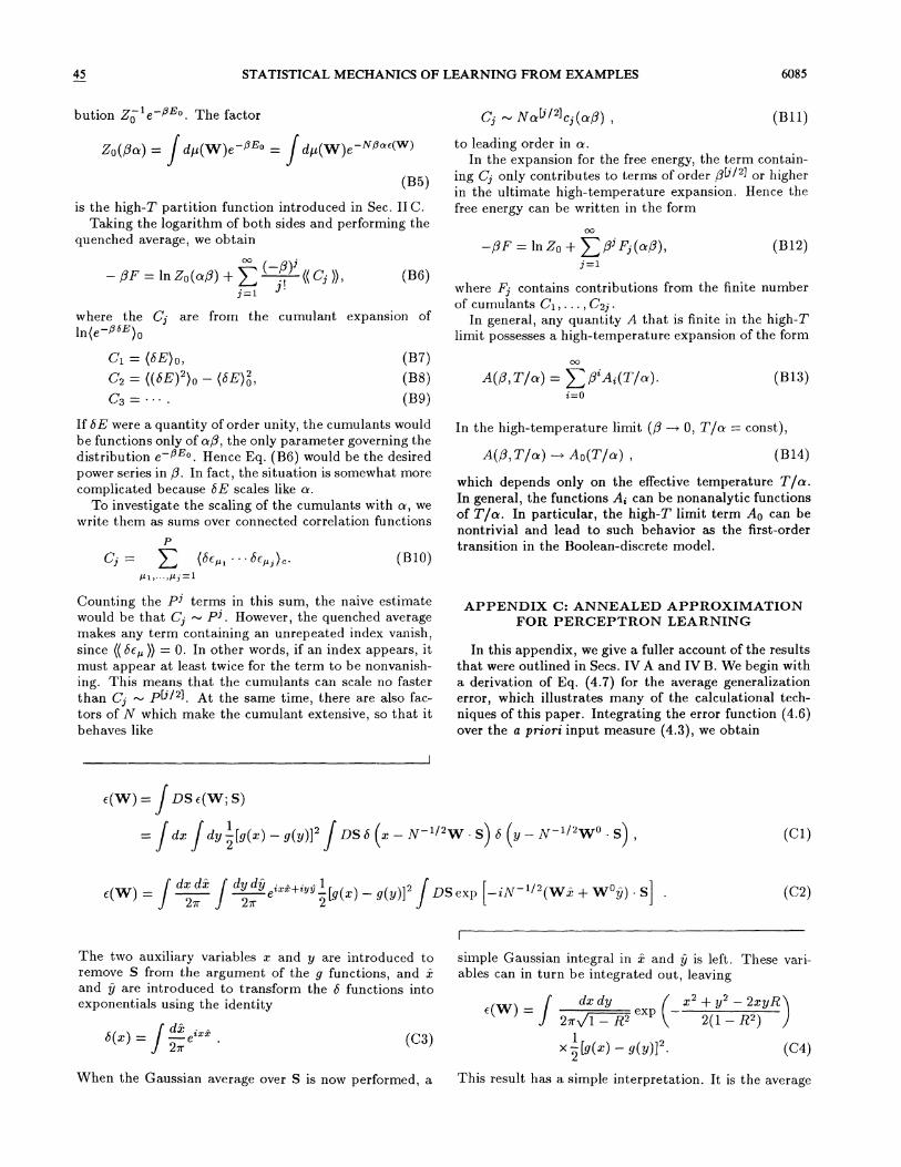
STATISTICAL MECHANICS OF LEARNING FROM EXAMPLES 6085
bution Zo e ~ '. The factor C, - NnL ~'lc, (nP), (811)
S ()lz) = f dy(W)e g ' = f dy(W)e
(85)
is the high-7 partition function introduced in Sec. II C.Taking the logarithm of both sides and performing the
quenched average, we obtain
—PF = InZp(nP) ~ ) ., ((C, }},
- (—P)'
j=lwhere the Ci are from the cumulant expansion of
to leading order in n.In the expansion for the free energy, the term contain-
ing Ci only contributes to terms of order PL))'2l or higherin the ultimate high-temperature expansion. Hence thefree energy can be written in the form
PF—= ln Zp+ ) P F (nP),j=l
(812)
where F& contains contributions from the finite numberof cumulants C), . . . , Cqi.
In general, any quantity A that is finite in the high-Tlimit possesses a high-temperature expansion of the form
Cg ——(b E}p,
C = ((b&)'} —(b&}'~ ~ ~
(87)(88)(89)
A(P, T/o() = ) P'A;(T/n).i=0
(813)
If bE were a quantity of order unity, the cumulants wouldbe functions only of esp, the only parameter governing thedistribution e ) '. Hence Eq. (86) would be the desiredpower series in P. In fact, the situation is somewhat morecomplicated because bE scales like o. .
To investigate the scaling of the cumulants with o. , we
write them as sums over connected correlation functions
P
) (be„, be„,},. .
)t 1) ~ . .)Pg =1(810)
Counting the P& terms in this sum, the naive estimatewould be that C& P~. However, the quenched averagemakes any term containing an unrepeated index vanish,since ((be& )} = 0. In other words, if an index appears, itmust appear at least twice for the term to be nonvanish-ing. This means that the cumulants can scale no fasterthan C& P~~ ~. At the same time, there are also fac-tors of N which make the cumulant extensive, so that itbehaves like
In the high-temperature limit (P ~ 0, T/og = const),
A(P, T/cy) ~ Ap(T/n), (814)
APPENDIX C: ANNEALED APPROXIMATIONFOR PERCEPTRON LEARNING
In this appendix, we give a fuller account of the resultsthat were outlined in Secs. IV A and IV B. We begin witha derivation of Eq. (4.7) for the average generalizationerror, which illustrates many of the calculational tech-niques of this paper. Integrating the error function (4.6)over the a priori input measure (4.3), we obtain
which depends only on the effective temperature T/cdIn general, the functions A; can be nonanalytic functionsof T/od. In particular, the high-T limit term Ap can benontrivial and lead to such behavior as the first-ordertransition in the Boolean-discrete model.
e(W) =jDS e(W', S)
1dz dy —(g(z) —g(y)] fDSg (z —N & W S) g (y —N ~ W S), (C1)
dgdp . - -1 —1 2 " 0-2~ 2
e' +'""—Ig(z) —g(y)] DS exp iN '~ (Wi + W—y) . S (C2)
b(z) = —e'z~~
2x (C3)
The two auxiliary variables x and y are introduced toremove S from the argument of the g functions, and xand y are introduced to transform the 6 functions intoexponentials using the identity e(W) = dzdy z2+ y2 —2zyR)
2+v'I —R' 2(1 —R') )x —[g(z) —g(y)] . (C
simple Gaussian integral in x and y is left. These vari-ables can in turn be integrated out, leaving
When the Gaussian average over S is now performed, a This result has a simple interpretation. It is the average

6086 H. S. SEUNG, H. SOMPOLINSKY, AND N. TISHBY 45
of2 [g(z) —g(y)]2, where z and y, like W S/~N and W
S/~N in (4.6), are Gaussian variables with unit varianceand cross correlation R. A simple change of variables in
Eq. (C4), a shift followed by a rescaling, yields the form(4.7).
To derive the annealed approximation for perceptronlearning, we begin by evaluating Eq. (2.31) for G „(W).The calculation is essentially the same as the previousone for c(W), and results in a similar formula,
1Gp ———ln
N
%co dR. exp
~
N—RR
0)+ ln dp(W) e
AVe can write the stationarity equations in a more re-vealing form by proceeding further in the evaluation ofGp. The b function in (C8) can be expanded by intro-ducing another order parameter R,
G,„(W) = —lndz dy z2+ y~ —2zyR
2(1 —R')
exp( —P[g(z) —g(y)] /2) . (C5)
In the thermodynamic limit, this reduces to
G = —RR+ —ln dp(W) e
(C10)
(Cl1)
Again, the answer depends on W only through the over-lap R. A change of variables in the integral (C5) yieldsthe form (4.14). Evaluating the integral for the casesof g(z) = z (linear perceptron) and g(z) = sgn(z)/y 2(Boolean perceptron), we obtain
where the right-hand side must be stationary with re-spect to the saddle-point parameter R. The free energycan now be written as a saddle point over two order pa-rameters
A
Pf =—extr - RR+ ——ln dp(W) eR,R N
0 „= &ln [1 + 2P(1 —R)] (linear)
(C6)—ln [1 —(1 —e ~)7r i cos i R] (Boolean).
—nG „(R)
The saddle-point equations are
(C12)
(( Z)) = dRexp N[Gp(R) —nG, „(R)), (C7)
Although derived using the Gaussian a priori input dis-tribution (4.3), the above results for e(W) and G „(W)apply also to the case of the discrete inputs S; = klin the thermodynamic limit. This insensitivity to inputdistribution is explained by the central limit theorem,which guarantees that W S/~N and WP S/~N areGaussian variables (in the N ~ oo limit) with very weakassumptions about the distribution of S. This assertionmay be verified by a straightforward calculation for dis-crete S, which yields Eqs. (C6) as the leading terms in asaddle-point expansion in 1/N
Since G „(W), Eq. (2.31), depends only on the over-lap R, the annealed partition function (2.30) can now berewritten as an integral over R,
G„R
R= —(W)- W1 0
(C13)
(C14)
where
J dp(W) W exp(RW WP)
Idp(W) exp(RW WP)(C15)
The order parameter R has a natural interpretation: itis the strength of a local field pushing W in the directionof W . Since it increases with n, it forces W toward Wpas n ~ oo, Upon eliminating R, these equations reduceto Eq. (4.16).
Equation (Cll) can be evaluated quite easily for thecase of the Ising constraint lV; = +1. Then we can makethe replacement
where
NGp(R) = ln dp(W) b(R —N 'W W ) (C8)
dp(W) ~ )W, =+1
which leads finally to
Gp(R): —RR + In 2 cosh R
(C16)
(C17)is the logarithm of the density of networks with overlapR. In the thermodynamic limit (N ~ oo), the integralcan be evaluated as
assuming that the teacher weights also satisfy the Isingconstraint. Extremizing with respect to R, we obtain theequation
1P f (T, n) = ——ln(( Z )):extrR[Gp(R) —nGB~(R)] . R = tanhR (C18)
(C9)
Hence the thermodynamic free energy f(T, n) is deter-mined by extremizing the free-energy function Pf(R)=-Gp(R) —nG „(R). DifFerentiating f(R) with respect toR, we obtain the stationarity condition Eq. (4.16).
Eliminating R, one can finally derive the result (4.20),which is purely a function of R, and is the familiar resultfor the entropy of the Ising model as a function of themagnetization R.
Calculating Gp for the spherical distribution is some-what more complicated. We rewrite the a priori spherical

45 STATISTICAL MECHANICS OF LEARNING FROM EXAMPLES 6087
distribution (4.17) as
dW- 'dA(~) & A(W W N)—
:.-; g2n-e; 2+i (C19)
Eliminating R and A finally yields the result (4.18), whichwas justified previously by geometric arguments.
and then Go is determined as a saddle point over R andAPPENDIX D: REPLICA THEORY
OF PERCEPTRON LEARNING
Ge = ——1n(Pee) + RR+ i + 1n f dpPe2
1 - 1 g2= ——+ RR+ A ——ln(2A) +
2 2 4A(C20)
The starting point of the replica calculations is thederivation of the replicated Hamiltonian (2.49), whichresembles the derivation of the annealed G'» describedin Appendix C. We introduce auxiliary variables z, iy, and y in order to simplify the average over S,
e ~~ i= DSexp — eW;So'=1
dyexp -P).[g-( z) - g(y)]'2 )
n
DS 6 ~. —N-']'W'. S 6 y —N-'i'W' So=1
dz di dy dy i 1exp —— gz —gy +i z z +iyy~
x DSexp —i' &l W i~+W y l S
0'
(D1)
The average over S is now a simple Gaussian integral and yields
- —- dz~ dz dydy i 1e g"lq p' l = exp ——p ) [g(z ) —g(y)] + i ) z z + iyy
xexp —-) i iRQ R—y) i,R (D2)
Since Q„depends on the weights only through the order parameters Q z and R that were defined in Eqs. (2.55) and
(4.21), the replicated partition function can be written as an integral over these order parameters
((Z" )) = f dQ e f dR exp( —Rng, (Q e, R ])o(p CJ
x dpW 6 p S W 'W 6 R N W WC7 e(p CT
(D3)
((&")) = . . exp N(gp[Q R, R, Q R, R ] —ag„[Q R, R ]),dQ RdQ R dR dR
&p CT
where
ge= —) RR —) QeQe+ —Inf dP(W)exP ) RW W +) QeW Wee y(p e(p
(D4)
(D5)

6088 H. S. SEUNG, H. SOMPOLINSKY, AND N. TISHBY 45
is the logarithm of the density of replicated networks withthe overlaps Q~p and R .
In the thermodynamic limit, the integral (D3) over theorder parameters is dominated by the saddle point inQ p and R . The free energy is obtained by analyticallycontinuing this saddle point to n = 0,
R =R,Q p—- 6 p+(1 —6 p)q,R =R.
(D8)
(D9)
(D10)
With this substitutions, the free energy takes the form
—Pf = lim ln((Z" ))1
n o~+extr pe[Q, e, R„Q,r, tt, ] —rrtr„[Q, r, R,])Q p, R
(D6)
According to the RS ansatz, the saddle point takes theform
Pf—= extr[Gp(q, R, q, R) —nG„(q, R)],q, R
where we have defined
G„= lim —",n~0
0Go = lim-
n-+0
(Dl I)
(D12)
(D13)
Q p= ~ p+ (I - ~ p)q, (D7)
To calculate G„, we substitute the RS ansatz intoEq. (D2) and perform the integral over y, leaving
e ~"= Dydz. di.
2]l l 2--~ ) .b(*.) —q(~)]'
1 -2x exp ——(1 —q) ) i, +i) i, (z, —Ry) Dt exp —itgq —Rz) zd d
(D14)
The auxiliary variable & has been introduced via the identity f Dg e~' = exp(~ bz). performing the integrals over theid, and shifting and rescaling the zd integrals, we finally obtain
e ' = Dt Dg Dxexp ]
——p g xtt'1 —g+ gtt+ t/g —tt —g(g) )-g~ 2
2
Taking the limit n +0 gives -Eq. (4.27) for G„.The RS result for g[] is
1 1) 1 t'Qo
——n~
RR ——n(n ——1)qq ——q ~ + —ln Dz
~ dp(W) exp[W (z+q+ W R)] I2 2) N
The n ~ 0 limit of this expression yields Eq. (4.26) for Go.
(D15)
(D16)
APPENDIX E: ONE-STEP RSB FOR PERCEPTRONS
Following the Parisi theory of RSB [45] we make the following "one-step" ansatz for the form of the order parametermatrix Q]t tr
'.
(1 qy
1qo qo
qo qo
qo qo .qo qo . .
1 q1
1 1 (El)
Fach block in this structure is an m x m matrix. All off-diagonal blocks consist of Q]t„——qp. The diagonal block has
Q» —I and Q„, = q for p g v. The conjugate matrix Q&„has a similar block structure. The order parameters R„

45 STATISTICAL MECHANICS OF LEARNING FROM EXAMPLES 6089
and R„are symmetric at the saddle point, i.e. , R„=R and R„=R, as before.Upon replacing Eqs. (D7)—(D10) by the RSB ansatz and taking the appropriate n ~ 0 limit, the free energy (D6)
is given by
P—f = Go(qo, qi, qo, qi, R, R, ») —nG, (qo, qi R m),where
1 1Go = —{mqoqo + [(1 —m)qi —1]qi) —RR+
2 Nm
(E2)
(E3)
Z = zo Jqa + zi Qqi —qo + W R, (E4)
1G„= —— Dy Dtp ln Dti( 1
Dz exp~
——P[g(t) —g(y)]'2
(E5)
t —= toVqo —R +tiVqi —qo
—yR. (E6)
The free energy has to be minimized with respect to qp, qi, qp, qi, R, R, and ms Note that after the n —+ 0 limithas been taken the allowed range of m is 0 & m & 1. Also, the physical meaning of qp, q], and m is explained inSec. V D 2 [see Eqs. (5.73)—(5.75)]. Upon substituting m = 0, the free energy f reduces to the RS result, Eq. (5.66).
Specializing to the case of Ising constrained weights in Gp and Boolean output in Gi, we obtain
1Gp ———(mqpqp + [(1 —m)qi —1] qi) —RR
21+ ) Dzp ln
Nm
mDzi 2cosll zp~qp+ ziti —qp+ W R (E7)
2G
mDy Dtp ln Dti e ~ + (1 —e ~)H(r) (E8)
qp—R2
7 = $p + $y1 —q1
qs —qp
1 —qy
(E9)
We now search for a solution to the saddle-point equa-tions at finite temperature with the property
OO
G„= —— Dy Dtln e P + (1 —e P )H(u)m p
qy —1, qy =oo (E10) (E12)
According to Eq. (5.73), for such a solution each purephase consists of a single (or a few almost identical) mi-croscopic state. Thus the system collapses at finite tem-peratures to phases with zero entropy. This is not unlikethe collapse of the system to the ground state at highervalues of n (i.e., the perfect generalization state). How-ever, it occurs in the metastable, spin-glass regime.
To find a solution with the property (E10) we takethe limit qi ~ 1, qi ~ oo of Eqs. (E7) and (E9) whilekeeping P finite. We obtain
1Go = —[m qp(qp —1) —mRR]
m
+ ) fDzls2cosh (zm~q~+WcmR)
(E11)
qp —R2u=t1 —qp
yRgl —
qp(E13)
Comparing Eqs. (Ell)—(E13) with Eq. (5.66) one obtains
h A
fRsB(qo qo R R, m, P) = fns(qo, m qo, R, mR, pm)
qp(T, m, n) = qns(T/m, n),
R(T, n, m) = RRs (T/m, n) .
(E15)
(E16)
(E14)
This structure is similar to the result of Krauth andMezard [33] for the case of training a perceptron withrandom input-output mappings.
Stationarity with respect to qp, qp, R and R results in

6090 H. S. SEUNG, H. SOMPOLINSKY, AND N. TISHBY 45
Finally, stationarity with respect to rn yields
sRs(T/m, a) = 0,which implies
m(T, n) = T/Ts (o ),
(E17)
(E18)
where Ts(n) is the s = 0 line of the RS solution.%'e have not attempted to search for other RSB so-
lutions or to check the stability of this solution. How-ever, this solution is probably exact both here and inthe random perceptron problem of Krauth and Mezard.Similar completely frozen SG phases are known to ex-ist in the REM, the "simplest spin glass" [54], and thelarge-P Potts glass. Recently, they have also been foundin learning of random mappings by two-layer networks[60,62,63].
APPENDIX F: POWER COUNTINGIN THE HIGH- TEMPERATURE EXPANSION
For the Boolean-mismatched model, the optimal gen-eralization and zero entropy lines both follow power lawsof the form T e", with 0 ( r & 1. The determina-tion of this exponent requires the balancing of the twodominant terms in the asymptotic expansion. This issomewhat tricky, because determining which are the twodominant terms in turn depends on the exponent.
Since both T and n are diverging, it would seem nat-ural to perform a double expansion around (1/T, I/cr) =(0, 0). Such an expansion is in fact ill defined, since theexistence of a nontrivial high-temperature limit showsthat the T, n ~ oo limit depends on the ratio T/cx.
As discussed in Appendix B, the proper high-temperature expansion for a quantity A that is finite inthe high-T limit is
A(P, T/~) = ) P'A;(T/n) .
i=0(F1)
If one proceeds to expand the A;, one obtains a doubleexpansion about (1/T, T/n) = (0, 0)
A(I/T, T/n) = ).A i —i i
— . (F2)Ii'(TT)
This high-T expansion is the proper tool for investigatingpower laws of the form T o,". We must only assume
that 0 & r & 1, so that both 1/T and T/n approach zeroRS 0,' ~ OO.
Assuming now that we have an expression for e& ofthe form (F2), let us find the power law T zi n" suchthat es decreases at the fastest rate. In the series (F2)each term a, b scales like I/n"'+(i "&~, so that the expo-nent is some weighted average of a and b. The power ofthe dominant term in the sum is min;[ra; + (1 —r)b;].This exponent must be maximized, to ensure the fastestdecrease of e&.
The problem thus reduces to linear programming.Given a set of pairs (a, , b;), find the r that maximizesmin; [ra, + (1—r)b;]. The problem looks difficult becausethere are an infinite number of pairs (a, , b;) to consider,but in fact most of the pairs can be eliminated from con-sideration. We define a partial ordering of the set of pairs:(a;, b;) & (aJ, bz) means a; & a& and b; & b& Ate. rm(a, b) is minimal if (a, b) & (c, d) implies (a, b) = (c, d) forall (c, d). Only the subset of minimal pairs (which can-not be ordered) are relevant, because (a;, b, ) & (a&, b&)implies ra; + (1 —r)b; & ra& + (1 —r)bz The li. near pro-gramming problem thus only includes the finite minimalsubset of pairs (a;, b;)
For the Boolean-mismatched model, we calculated theasymptotics of the generalization error as a series inn-'~' at fixed T,
E'g (T~ cr) &min: ) ej /9(P)Aj=l
(F3)
To convert this to the form (F2) of the high-T expan-sion, we expand the e~. in powers of P. Only the leadingterm from each ej need be retained, since the higher-order terms are irrelevant. From the terms of order ethrough n ~ we obtain the (1, 1/2), (1, 1), (1,3/2), and(0, 2) terms in the high-T expansion (F2). From thesefour terms, we finally extract the minimal subset (1, 1/2)and (0, 2). Terms in (F3) of order n s~~ and higher neednot be considered, since they are all bounded below by(0, 2) and are thus irrelevant.
The maximin problem, which involves only (1, 1/2) and(0, 2), has r = 3/5 as its solution, justifying the resultToi,& n ~ quoted in Eq. (6.54). The calculation ofthe zero-entropy line is similar, except that the minimalterms must add up to zero.
Present address: Department of Computer Science, He-brew University, Jerusalem 91904, Israel.
[1] R. P. Lippman, Neural Comput. 1, 1 (1989).[2] T. J. Sejnowski and C. Rosenberg, Complex Syst. 1, 145
(1987).[&] Y «Cun, B. Hoser, J. S. Denker, D. Henderson, R. E.
Howard, W. Hubbard, and L. D. Jackel, Neural Comput.1, 541 (1989).
[4] N. gian and T. J. Sejnowski, J. Mol. Biol. 202, 865(1988).
[5] D. Zipser and R. A. Andersen, Nature 331, 679 (1988).[6] S. R. Lockery, G. Wittenberg, Jr. , W. B. Kristan, and
W. G. Cottrell, Nature 340, 468 (1989).[7] Parallel Distributed Processing: Explorations in the Mi
crostructure of Cognition, edited by D. E. Rumelhart andJ. L. McClelland (MIT Press, Cambridge, MA, 1986).
[8] T. Poggio and F. Girosi, Proc. IEEE 78, 1481 (1990).[9] L.G. Valiant, Commun. ACM 27, 1134 (1984).
[10] A. Blumer, A. Ehrenfeucht, D. Haussler, and M. K. War-
muth, J. ACM 36, 929 (1989).[11] E. Baum and D. Haussler, Neural Comput. 1, 151 (1989).[12] D. Haussler, Inf. Computation (to be published).[13] S. Judd, J. Complexity 1, 177 (1988).[14] V. N. Vapnik and A. Y. Chervonenkis, Theory Probab.

45 STATISTICAL MECHANICS OF LEARNING FROM EXAMPLES
Appl. 16, 264 (1971).[15] V. N. Vapnik, Estimation of Dependences Based on Em-
pirical Data (Springer-Verlag, New York, 1982).[16] Y. S. Abu-Mostafa, Neural Comput. 1, 312 (1989).[17] A. R. Barron, in Proceedings of the 88th Conference on
Decision and Control (IEEE Control Systems Society,New York, 1989), Vol. 1, pp. 280—285.
[18] L. Devroye, IEEE Trans. Pattern Anal. Mach. Intell. 10,530 (1988).
[19] P. Carnevali and S. Patarnello, Europhys. Lett. 4, 1199(1987).
[20] N. Tishby, E. Levin, and S. Solla, in Proceedings of the International Joint Conference on Neural Networks (IEEE,New York, 1989), Vol. 2, pp. 403—409.
[21) E. Levin, N. Tishby, and S. A. Solla, Proc. IEEE 78,1568 (1990).
[22] P. del Giudice, S. Franz, and M. A. Virasoro, J. Phys.(paris) 50, 121 (1989); D. Hansel and H. Sompolinsky,Europhys. Lett. 11, 687 (1990).
[23] E. Gardner and B. Derrida, J. Phys. A 22, 1983 (1989).[24] G. Gyorgyi and N. Tishby, Neural Networks and Spin
Glasses, edited by W. K. Theumann and R. Koberle(World Scientific, Singapore, 1990), pp. 3—36.
[25] G. Gyorgyi, Phys. Rev. Lett. 64, 2957 (1990).[26] W. Krauth, M. Mezard, and J.-P. Nadal, Complex Syst.
2, 387 (1988).[27] J. A. Hertz, in Statistical Mechanics of Neural Networks:
Proceedings of the Eleventh Sitges Conference, edited byL. Garrido (Springer, Berlin, 1990), pp. 137—153.
[28] D. B. Schwartz, V. K. Samalam, J. S. Denker, and S. A.Solla, Neural Comput. 2, 374 (1990).
[29] J. Shrager, T. Hogg, and B. A. Huberman, Science 242,414 (1988).
[30] J. Denker, D. Schwartz, B. Wittner, S. Solla, R. Howard,L. Jackel, and 3. Hopfield, Complex Syst. 1, 877 (1987).
[31] E.L. Thorndike, Fundamentals of Learning (ColumbiaUniversity Press, New York, 1932).
[32] W. Kohler, Gestalt Psychology (Liveright, New York,1929).
[33] W. Krauth and M. Mezard, J. Phys. (Paris) 50, 3057(1989).
[34] S. S. Venkatesh, in Proceedings of the Fourth AnnualWorkshop on Computational Learning Theory, edited byM.K. Warmuth and L.G. Valiant (Kaufmann, San Ma-teo, CA, 1991), pp. 257—266.
[35] H. Sompolinsky and N. Tishby, Europhys. Lett. 13, 567(1990).
[36] I. Kocher and R. Monasson (unpublished).[37] H. Sompolinsky, N. Tishby, and H. S. Seung, Phys. Rev.
Lett. 65, 1683 (1990).[38] K. Binder and D. W. Heerman, Monte Carlo Simulation
in Statistical Mechanics (Springer-Verlag, Berlin, 1988).[39] S. Kirkpatrick, Jr. , C. D. Gelatt, and M. P. Vecchi, Sci-
ence 220, 671 (1983).[40] S. F. Edwards and P. W. Anderson, 3. Phys. F 5, 965
(1975).[41] D. Sherrington and S. Kirkpatrick, Phys. Rev. Lett. 35,
1792 (1975).[42] S. Kirkpatrick and D. Sherrington, Phys. Rev. B 17, 4384
(1978).[43] H. Sompolinsky, Phys. Rev. Lett. 47, 935 (1981).[44] K. Binder and A. P. Young, Rev. Mod. Phys. 58, 801
(1986).[45] M. Mezard, G. Parisi, and M.A. Virasoro, Spin Glass
Theory and Beyond (World Scientific, Singapore, 1987).[46] F. Rosenblatt, Principles of Neurodynamics (Spartan,
New York, 1962).[47] J. R. L. de Almeida and D. 3. Thouless, J. Phys. A 11,
129 (1978).[48] A. Krogh and J. A. Hertz, in Advances in Neural Infor
motion Processing Systems, edited by R. P. Lippman, J.E. Moody, and D.S. Touretzky (Kaufmann, San Mateo,CA, 1991), pp. 897-903; J. Phys. A (to be published).
[49] M. L. Minsky and S. Papert, Perceptrons (MIT Press,Cambridge, MA, 1988).
[50] M. Opper and D. Haussler, Phys. Rev. Lett. 66, 2677(1991).
[51] M. Opper and D. Haussler, in Proceedings of the FourthAnnual Workshop on Computational Learning Theory(Ref. [34]), pp. 75—87.
[52] E. Gardner, J. Phys. A 19, L1047 (1986).[53] G. Gyorgyi, Phys. Rev. A 41, 7097 (1990).[54] B. Derrida, Phys. Rev. B 24, 2613 (1981).[55] B. Derrida, R. B. Gri%ths, and A. Prugel-Bennett, J.
Phys. A 24, 4907 (1991).[56] J. F. Fontanari and R. Meir, Network 2, 353 (1991).[57] T. M. Cover, IEEE Trans. Electron. Comput. 14, 326
(1965).[58] E. Gardner, J. Phys. A 21, 257 (1988).[59] E. Gardner and B. Derrida, 3. Phys. A 21, 271 (1988).[60] E. Barkai, D. Hansel, and I. Kanter, Phys. Rev. Lett. 65,
2312 (1990).[61] J. F. Fontanari and R. Koberle, J. Phys. (Paris) 51, 1403
(1990).[62] E. Barkai, D. Hansel, and H. Sompolinsky, Phys. Rev. A
45, 4146 (1992).[63] E. Barkai and I. Kanter, Europhys. Lett. 14, 107 (1991).