statistical machine learningfor data mining and …lyu/student/phd/steven/defense_hoi.pdf1...

1

Statistical Machine Learningfor Data Mining and

Collaborative Multimedia Retrieval

Presented by Steven C.H. Hoi

Supervisor: Prof. Michael R Lyu

The Chinese University of Hong Kong

Date: 28 Aug, 2006Time: 4:00 – 6:00 p.m.

Ph.D. Defense Presentation, CSE Dept, CUHK

2

OutlineBackgroundContributionsLearning Unified Kernel MachinesBatch Mode Active LearningCollaborative Multimedia RetrievalConclusionsFuture Work

Statistical Machine Learning for Data Mining and Collaborative Multimedia Retrieval

3

Background

Statistical Machine LearningSupervised LearningUnsupervised LearningSemi-Supervised LearningActive LearningDistance Metric LearningOthers (reinforcement learning, etc.)


4

Background

Challenging IssuesHow to unify a variety of machine learning techniques in an effective fashion?How to perform active learning efficiently and effectively?How to learn distance metrics from context data?How to develop appropriate metric learning techniques for real-world applications?


5

ContributionsLearning Unified Kernel Machines

Spectral Kernel LearningUnified Kernel Logistic RegressionKernel Design via Marginalized KernelPublications: KDD 06, WWW 06

Batch Mode Active LearningBMAL for Text and Image CategorizationPublications: ICML 06, WWW 06

Distance Metric LearningDiscriminative Component Analysis (DCA) and KDCAPublication: CVPR 06

Collaborative Multimedia RetrievalLearning Log-Based Relevance FeedbackLearning Reliable Distance MetricsPublications: MM04, EMMA 05, TKDE 06, MMSJ 06


6

Overview of ContributionsLabeled Data

Unlabeled Data

Semi-SupervisedKernel Learning

Active Learning

DistanceMetric Learning

Unsupervised Learning

Kernel Initialization

Log Data(Context)

DCA / KDCA

Noise

RDML

Collaborative Multimedia Retrieval

Unified Kernel Machines

Batch Mode Active Learning

Marginalized Kernels

Web and Multimedia Data Classification

Statistical Machine Learning for Data Mining and Multimedia Retrieval

Web Mining

2

7

Part I: Learning Unified Kernel Machines

Motivation of Our FrameworkKernel machines play an important role in the state-of-the-art machine-learning techniques for data mining.Supervised Learning

Support Vector Machines (SVM)Kernel Logistic Regressions (KLR)Regularized Least-Square Classifiers (RLS)

Unsupervised Learning Spectral Clustering, Kernel PCA, …

Active LearningMargin-Based Active Learning with Kernel Machines, etc.

How to combine these kernel machine-learning techniques in a unified solution?

Part I: UKM

8

Learning Unified Kernel MachinesA Unified Framework

KernelInitialization

Semi-Supervised Kernel LearningActive Learning Model Parameters

Estimation

Convergence Evaluation

Unified Kernel Machine

Standard kernels(Linear, Poly, RBF)

Domain-Specific kernels(Graph, Sequence, Tree)

Part I: UKM

9

Semi-Supervised Kernel Learning

GoalTo learn an effective kernel (matrix) from both labeled and unlabeled data

Theoretical PrinciplesUnsupervised Kernel Design

Learning Kernel from unlabeled dataKernel Target Alignment

Learning Kernel from labeled data

Part I: UKM

10

Semi-Supervised Kernel LearningOverview of Kernel Machine Learning

Supervised LearningGiven l training examples (x1,y1), … (xl, yl), one can train a prediction function p in the RKHS by the following formula

The solution of (1) can be represented as:Empirical loss term Regularization term

(1)

(2)

Part I: UKM

11

Semi-Supervised Kernel LearningOverview of Kernel Machine Learning

Semi-Supervised LearningGiven l training examples (x1,y1), … (xl, yl), and (n-l) unlabeled data examples (xl+1, xl+2,…,xn), let f be n-dimensional real vector, which is learned by the following semi-supervised learning method:

Theorem (Zhang et al., NIPS’05): The solution of (3) is equivalent to the solution of (1):

(3)

Part I: UKM

12

Unsupervised Kernel Design

The equivalence theorem shows that, in order to exploit the unlabeled data, we can consider the following supervised learning approach with unsupervised kernel design:

(1) Design a new kernel K’ using unlabeled data(2) Apply the new K’ in the supervised learning formula

Spectral Kernel Design

Principle: A kernel with faster spectra decay should be more preferred. (Zhang et al., NIPS’05)

Part I: UKM

3

13

Kernel Target Alignment

Kernel Alignment (Cristianini et al. 2002): The empirical alignment of two given kernels K1 and K2 with respect to a sample set is the following quantity:

where

Target KernelLet y=[y1,…,yl]’ be a label vector of training data, for binary classification, the target kernel can be defined as:

Part I: UKM

T

1 1 11 1 1

1 1 1T

−⎛ ⎞⎜ ⎟= = − −⎜ ⎟⎜ ⎟−⎝ ⎠

yy[ ]T1 1 1= − −y

14

Kernel Target Alignment

Let K the kernel matrix of all data, which can be represented as the following structure

Principle: A better kernel can be optimized by maximizing the following kernel target alignment:

Part I: UKM

15

Spectral Kernel Learning

PrinciplesMaximizing kernel target alignment meanwhile keeping fast spectra decay!

Formulation of Algorithm

C is a decay factor to enforce a faster decay rate of spectra (C>=1)

top d eigenvectors of initial kernel

Part I: UKM

16

Spectral Kernel LearningFormulation of Algorithm (cont’)

Let

Part I: UKM

fix numerator to1

17


Formulation of Algorithm (cont’)

This is a standard Quadratic Programming (QP) problem.

Part I: UKM

18

Spectral Kernel LearningConnections to Other Kernel Techniques

Spectral Kernel Learning (SKL)

Cluster Kernel ([1, …,1, 0, …,0], Spectral Clustering)

Truncated Kernel (top eigen components, Kernel PCA)

When setting C=1, d=n, and assuming the initial kernel K is constructed from graph laplacian L, our SKL method is equivalent to the order-constrained graph kernel (Jerry Zhu, NIPS’2005)

Part I: UKM

4

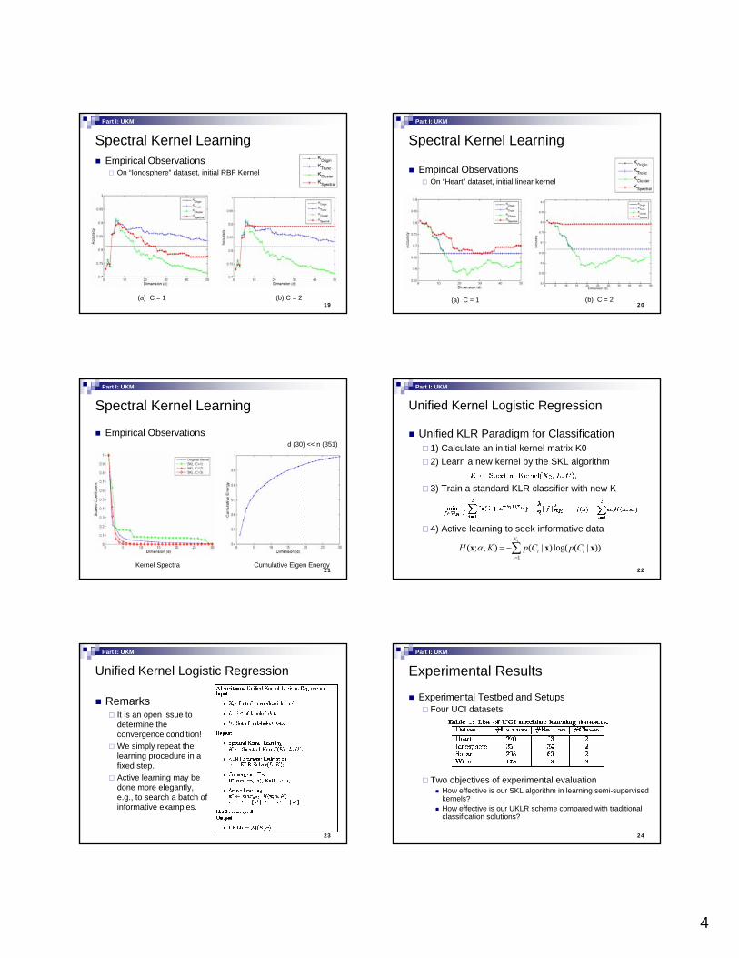
19

Spectral Kernel LearningEmpirical Observations

On “Ionosphere” dataset, initial RBF Kernel

(a) C = 1 (b) C = 2

Part I: UKM

20


Empirical ObservationsOn “Heart” dataset, initial linear kernel

(a) C = 1 (b) C = 2

Part I: UKM

21


Empirical Observations

Kernel Spectra Cumulative Eigen Energy

d (30) << n (351)

Part I: UKM

22

Unified Kernel Logistic Regression

Unified KLR Paradigm for Classification 1) Calculate an initial kernel matrix K02) Learn a new kernel by the SKL algorithm

3) Train a standard KLR classifier with new K

4) Active learning to seek informative data

Part I: UKM

1

( ; , ) ( | ) log( ( | ))CN

i ii

H K p C p Cα=

= −∑x x x

23

Unified Kernel Logistic Regression

RemarksIt is an open issue to determine the convergence condition!We simply repeat the learning procedure in a fixed step.Active learning may be done more elegantly, e.g., to search a batch of informative examples.

Part I: UKM

24

Experimental Results

Experimental Testbed and SetupsFour UCI datasets

Two objectives of experimental evaluationHow effective is our SKL algorithm in learning semi-supervised kernels?How effective is our UKLR scheme compared with traditional classification solutions?

Part I: UKM

5

25


Semi-Supervised Kernel LearningCompared Kernels

3 standard kernels Linear, Quadratic, RBF

5 semi-supervised kernels3 SKL methods with different initial kernels2 Order-constraint graph kernels

Standard KLR classifier for classificationSettings

Fix decay factor C (C>1)Set dimension cut-off d = 2020 trials for each experimental comparison

Part I: UKM

26

Experimental ResultsSemi-Supervised Kernel Learning

Table 2. Classification performance of different kernels using KLR classifiers on UCI datasets. The mean accuracies and standard errors are shown in the table. Each cell in the table has two rows. The upper row shows the test set accuracy with standard error; the lower row gives the average time used in kernel learning.

Part I: UKM

27

Experimental ResultsSemi-Supervised Kernel Learning (cont’)

Part I: UKM

28


Unified Kernel MachinesCompared Schemes

KLR (initial classifier)KLR + Rand (initial KLR classifier with additional labeled examples sampled randomly)KLR + Active (initial KLR classifier with additional labeled examples by active learning)UKLR (Unified Kernel Logistic Regression)

Part I: UKM

29

Experimental ResultsUnified Kernel Machines

Part I: UKM

Table 3: Classification performance of different classification schemes on four UCI datasets. The meanaccuracies and standard errors are shown in the table. “KLR” represents the initial classifier with the initial train size; other three methods are trained with additional 10 random/active examples.

30

Summary of Part I

We presented a framework of learning unified kernel machines (UKM) for classification. A new semi-supervised kernel learning algorithm was proposed, which is related to an equivalent quadratic programming (QP) problem. A classification paradigm was developed by applying our UKM framework on the KLR model. Empirical evaluations are conducted on several UCI datasets.

Part I: UKM

6

31

Part II: Batch Mode Active Learning for Text Categorization

MotivationText CategorizationLogistic Regression and Active Learning

Batch Mode Active LearningTheoretical FoundationConvex Optimization FormulationEigen Space Simplification Bound Optimization Algorithm

Experimental ResultsSummary

Part II: BMAL

32

Motivation

Text CategorizationProblem: assign documents to predefined topicsSignificances

Core Web data mining techniqueApplications: category browsing, vertical search, etc.

Challenges To build efficient classifiersTo minimize human labeling effort

Part II: BMAL

33

Motivation

Logistic RegressionEfficiency for Training and PredictionNatural Probability OutputState-of-the-art performance, etc…Linear model

where is the class label.Simplified notation:

Part II: BMAL

34

MotivationActive Learning

Goal: to find most informative unlabeled dataTraditional Methodology

Choose one unlabeled example for labeling Retrain the classifier with the additional exampleLimitation: only one example, large retraining cost

Batch Mode Active LearningTo find a batch of most informative unlabeled examples

Part II: BMAL

35

Batch Mode Active Learning

(a) Binary classification example (b) Margin-based active learning (c) Batch mode active learning

– Positive examples of class-1– Negative examples of class-2

– Unlabeled examples– Selected examples for labeling

Toy Example

D1

D2

Part II: BMAL

36

Theoretical Foundation

Main Idea:Based on the theoretical framework of maximization of Fisher information

Problem SettingIn a probabilistic classification framework, assume the classification model is a semi-parametric form

For example, the logistic regression model:

Part II: BMAL

7

37

Theoretical Foundation

The problem of batch mode active learning can be regarded as a problem to seek a resample distribution q(x) of the unlabeled data.The examples with large resampling probabilities will be selected as the most informative ones for labeling. According to statistical estimation theory, active learning should consider a resample distribution q(x) that maximizes the following Fisher information

Part II: BMAL

38

Theoretical FoundationThe maximization of Fisher information is equivalent to find the resample distribution q(x) that minimizes the ratio of two Fisher information matrixces:

For the logistic regression model, the Fisher information matrix can be expressed as:

We replace the integration in the above equation with the summation over the unlabeled data:

Part II: BMAL

39

Convex Optimization FormulationRewrite the objective function as

Introduce a slack matrix ,then turn the original problem into the following optimization:

In the above, we use

Part II: BMAL

40

Convex Optimization FormulationBy the Schur complementary theorem, i.e.,

we turn it into the following optimization :

Part II: BMAL

41

Convex Optimization FormulationThe final optimization problem can be expressed

The above problem belongs to the family of Semi-definite programming (SDP) and can be solved by convex optimization techniques.

Part II: BMAL

42

Eigen Space Simplification

Directly solving the above optimization problem may be computationally expensive for the large-size slack matrix variable of M.In order to reduce the computational complexity, we propose an Eigen space simplification method to make the solution simpler and more effective. We assume that M is expanded in the Eigen space of the Fisher information matrix Ip.

Part II: BMAL

8

43


Let be the top s eigen vectors of the Fisher information matrix Ip, where λ1 ≥λ2 ≥ . . . ≥λs, then we assume the matrix M has the following form:

The inequality can be rewritten as:

Part II: BMAL

44


Using the eigen expression, we have

Since the necessary condition for

we then have the following result

Part II: BMAL

45


The previous necessary condition leads to following constraints:

Meanwhile, the objective function of tr(M) can be expressed as

Part II: BMAL

46


By putting the above two expressions together, we transform the SDP problem into the following approximate optimization problem:

Note that the above optimization problem belongs to convex optimization since f(x) = 1/x is convex when x ≥ 0.

Part II: BMAL

47

Bound Optimization Algorithm

Lemma 1: Let L(q) be the objective function,

we have the following conclusion:

Proof in Appendix.

Part II: BMAL

48


Given the lemma 1, now instead of optimizing the original objective function L(q), we can optimize its upper bound using simple updating equations:,

This algorithm will guarantee to converge to a local optimal. Since the original problem is a convex optimization problem, the above updating procedure will guarantee to converge to a global optimal.

Part II: BMAL

9

49


The updating step:

Some Observations(i) The example with a large classification uncertaintywill be assigned with a large probability.

(ii) The example that is similar to many unlabeled examples is more likely to be selected.

Part II: BMAL

50

Experimental Testbeds3 standard text datasets

Reuters-21578 dataset (10788)Two web-related datasets:WebKB (4518) and Newsgroup (10966)

Part II: BMAL

51

Experimental Settings

A standard feature selection by Information Gain is conducted toremove uninformative features, in which 500 of the most informative features are selected.The F1 metric is adopted as our evaluation metric, which has been shown to be more reliable metric than other metrics such as the classification accuracy. More specifically, the F1 is defined as

where p and r are precision and recall.Parameters of LogReg and SVM are determined by a standard cross validation method.

Part II: BMAL

52

Comparison SchemesTwo popular active learning methods:

SVM-AL: the classification uncertainty of an example x is determined by its distance to the decision boundary

The smaller the distance d(x;w, b) is, the more the classification uncertainty will be.LogReg-AL: the logistic regression active learning algorithm that measures the classification uncertainty based on the entropy of the distribution p(y|x).

The larger the entropy of x is, the more uncertain we are about the class labels of x.Our Batch Mode Active Learning algorithm with logistic regression, i.e., LogReg-BMAL in short.

Part II: BMAL

53

Empirical EvaluationExperimental Results with Reuters-21578

average results over 40 executions100 training examples and 100 active examples

Part II: BMAL

54

Empirical EvaluationExperimental Results with Reuters-21578

Part II: BMAL

10

55

Empirical Evaluation

Experimental Results with Web-KB Dataset

Part II: BMAL

56


Experimental Results with Newsgroup Dataset

Part II: BMAL

57

Summary of Part IIA new active learning scheme is suggested for text categorization to overcome the limitation of traditional active learning;A batch mode active learning solution is formulated by convex optimization techniques;An effective bound optimization algorithm is proposed to solve the batch mode active learning problem.Extensive experiments are conducted for empirical evaluations in comparisons with state-of-the-art active learning approaches for text categorization

Part II: BMAL

58

Collaborative Multimedia Retrievalvia Regularized Distance Metric Learning

Problem DefinitionCollaborative Multimedia Retrieval (CMR)is a Multimedia Information Retrieval (MIR) problem which involves human interactions, either with online relevance feedback explicitly or with historical log data of users’relevance feedback implicitly.

Part III: CMR

59

MotivationRelevance Feedback

A powerful tool for multimedia information retrievalPopular methods: SVM Based solutions

Log-based Relevance Feedback (LRF)Combining log data for online relevance feedbackOur contribution: Soft Label SVM for LRF (MM 04, TKDE 06)

Learning Distance Metrics with Log DataOur contribution: Regularized Distance Metric Learning for learning robust and scalable metrics (ACM MM Journal 06)

Part III: CMR

60

Regularized Distance Metric Learning

OverviewThe basic idea of this work is to learn a desired distance metric in the space of low-level image features that effectively bridges the semantic gap.It is learned from the log data of user relevance feedback based on the Min/Max principle, i.e., minimize/maximize the distance between similar/dissimilar images.

Part III: CMR

11

61

Regularized Distance Metric LearningFormulation

The log data are given in terms of log sessions. Each log session: each image was marked either relevant (+1), irrelevant (-1), or unknown (0).

+N

Log Session (Q)

Image examples in the database

1 -1 1 -1 -1 0 1 -1 -1 11

-1 1 -1 -1 -1 -1 -1 1 -1-10

Part III: CMR

62

FormulationWe first exploit a metric learning algorithm for log data

This formulation tells us:When two images are judged as relevant in the same log session, they could be similar to each other;When one image is judged as relevant and another is judged as irrelevant in the same log session, they must be dissimilar to each other.

Where Q stands for number of log sessions in the log data.

Part III: CMR

63

FormulationThe formulation in (4) may not be robust for noise, we form a new objective function for distance metric learning that takes into account both the discriminative issue and the robustness issue as:

(6)

Part III: CMR

64

FormulationUsing distance expressions, both the second and the third items of objective function in (5) can be expanded into the following forms:

Part III: CMR

65

FormulationPutting Eqn. (6), (7), (8) together, we have the final formulation for the regularized metric learning:

Part III: CMR

66

Formulation

To convert the above problem into the standard form, we introduce a slack variable t that upper bounds the Frobenius norm of matrix A, which leads to an equivalent form of (9), i.e.,

The first constraint is called a second order cone constraintThe second constraint is a positive semi-definite constraint.A special form of Convex optimization problems!There exists efficient solutions to solve it in a polynomial time

Part III: CMR

12

67


Datasets20-Category50-Category

Image Representation9-dimensional Color Histogram18-dimensional Edge Histogram9-dimension texture

Part III: CMR

68


Collection of Users’ Log Data

Part III: CMR

69

Experimental ResultsCompared Schemes:

1) “Euclidean”: Euclidean metric without log data.2) “IML”: based on the semantic representation learned from the manifold learning algorithm.3) “DML”: based on the metric learned by a typical distance metric learning algorithm.4) “RDML”: based on the metric by proposed regularized metric learning algorithm.

Part III: CMR

70

Experimental ResultsTable 2: Average precision (%) of top-ranked images on the 20-Categorytestbed over 2,000 queries. The relative improvement of algorithm IML,DML, and RDML over the baseline Euclidean is included in the parenthesisfollowing the average accuracy.

Table 3: Average precision (%) of top-ranked images on the 50-Category testbedover 5,000 queries.

Part III: CMR

71

Robustness EvaluationTable 4: Average precision (%) of top-ranked images on the 20-Categorytestbed for IML, DML, and RMDL using noisy log data. The relativeimprovement over the baseline Euclidean is included in the parenthesisfollowing the average accuracy.

Table 5: Average precision (%) of top-ranked images on the 50-Categorytestbed for IML, DML, and RMDL using noisy log data.

Part III: CMR

72

Efficiency and Scalability

Table 6: The training time cost (CPU seconds) of three algorithms on 20-Category (100 log sessions) and 50-Category (150 log sessions) testbeds.

Part III: CMR

13

73

Summary of Part IIIWe proposed a novel algorithm for distance metric learning, which boosts the retrieval accuracy of CBIR by taking advantage of the log data of users’relevance judgments. A regularization mechanism is used in the proposed algorithm to improve the robustness of solutions, when the log data is small and noisy. It is formulated as a positive semi-definite programming problem, which can be solved efficiently.Experiment results have shown that the proposed algorithm for regularized distance metric learning substantially improves the retrieval accuracy of the baseline CBIR system.

Part III: CMR

74

Summary of Other Contributions

Distance Metric Learning for ClusteringDiscriminative Component Analysis (DCA)Kernel DCA for learning nonlinear metricsDetails in Appendix A

Marginalized Kernels for Web MiningTime-dependent similarity measure schemeMarginalized kernels to exploit both explicit similarity and implicit cluster semantic for similarity measureDetails in Appendix B

75

ConclusionsWe proposed a framework of statistical machine learning for data mining and collaborative multimedia retrieval.We suggested a unified framework to learn the unified kernel machines, in which a new semi-supervised kernel learning algorithm was proposed. We explored the batch mode active learning problem and proposed a novel algorithm to search a batch of informative examples.We studied a real-world application, collaborative multimedia retrieval, and proposed a regularized distance metric learning algorithm for learning robust and scalable metrics for multimedia retrieval.

76

Future Work

Theoretical Analysis on UKM …More effective algorithms and extensions to UKM …Employing UKM to solve real-world problems, classification, regressions, information retrieval, …

77

Selected Publications (Regular Papers)1. "Learning the Unified Kernel Machines for Classification," Steven C.H. Hoi, Michael R. Lyu, Edward Y Chang,

In ACM SIGKDD (KDD2006), Philadelphia, USA, August 20 - 23, 2006.

2. “Large-Scale Text Categorization by Batch Mode Active Learning,” Steven C.H. Hoi, R. Jin and M.R. Lyu, In WWW 2006, Edinburgh, England, UK, 2006.

3. "Time-Dependent Semantic Similarity Measure of Queries Using Historical Click-Through Data", Q. Zhao, Steven C. H. Hoi, T.-Y. Liu, et al, In WWW 2006, May 2006.

4. "Batch Mode Active Learning and Its application to Medical Image Classification“, Steven C.H. Hoi, R. Jin, J. Zhu and M.R. Lyu, In ICML 2006, Pittsburgh, US, June 25-29, 2006.

5. “Learning Distance Functions with Contextual Constraints for Image Retrieval“, Steven C.H. Hoi, W. Liu, Michael R Lyu, W-M. Ma, in IEEE CVPR 2006, New York, June, 2006

6. "A Unified Log-based Relevance Feedback Scheme for Image Retrieval," Steven C. H. Hoi, Michael R. Lyuand Rong Jin, In IEEE Transactions on KDE (TKDE), vol. 18, no. 4, 2006

7. "Collaborative Image Retrieval via Regularized Metric Learning“, Luo Si, Rong Jin and Steven C. H. Hoi and Michael R. Lyu, ACM Multimedia Systems Journal (MMSJ), Special issue on Machine Learning Approaches to Multimedia Information Retrieval, 2006.

8. "A Semi-Supervised Active Learning Framework for Image Retrieval," Steven C. H. Hoi and Michael R. Lyu, in IEEE CVPR 2005, San Diego, CA, USA June 20-25, 2005

9. "A Unified Machine Learning Paradigm for Large-Scale Personalized Information Management,“, Edward Y. Chang, Steven C. H. Hoi, Xinjing Wang, Wei-Ying Ma and Michael R. Lyu, EIT 2005, NTU Taipei, August 2005.

10. "A Novel Log-based Relevance Feedback Technique in Content-based Image Retrieval," Steven C.H. Hoi and Michael R. Lyu, ACM Multimedia, New York, pp. 24-31, 2004 78

Thanks!

Q & A

14

79

Appendix

A: Distance Metric Learning for ClusteringB: Marginalized Kernels for Web MiningC: Proof of Lemma 1 in BMALD: Definition of Semi-Definite Programming

80

Appendix A:Distance Metric Learning for Clustering

MotivationWe address important limitations of existing metric learning methods, Relevant Component Analysis (RCA)It lacks of considering negative constraintsIt cannot capture nonlinear relationship of data instances via linear transformation

Solution:Discriminative Component Analysis (DCA)Kernel DCA to learn nonlinear metrics

81

Discriminative Component Analysis

FormulationGiven a set of data points and a set of contextual constraintsForm n chunklets using the positive constraints: Form a discriminative set to indicate which chunklets can be discriminated each other by the negative constraints.

1{ } jnj ji iC x ==

jD

1{ }Ni iX x ==

82


Two covariance matrixes are computed:

where , m_i is the mean of the i-th

chunklet, i.e., Finding the optimal transformation is equivalent to solve the following optimization:

1

1C ( )( )j

nT

b j i j ij i Db

m m m mN = ∈

= − −∑∑

1 1

1C ( )( )jnn

Tw ji j ji j

j iw

x m x mN = =

= − −∑∑

(1)

(2)

A

| A C A |(A) arg max| A C A |

Tb

Tw

J =

1| |

n

b jj

N D=

=∑1

1 in

i ijji

m xn =

= ∑

83


Algorithm for solving DCAIdea: Based on the Fisher’s criterion, the DCA problem can be solved by diagonalizing Cb and Cw simultaneously

Steps:1) Compute the covariance matrices Cb and Cw by Eq.(1),(2)2) Diagonalize Cb by eigenanalysis3) Project and diagonalize Cw by eigenanalysis4) Output transformation matrix A

A

| A C A|(A) argmax| A C A|

Tb

Tw

J =

84

Kernel DCA

The kernel techniques first map the input data into a feature space F.The data can be then analyzed in the projected feature space. The linear transformation in the feature space corresponds the nonlinear analysis in the input space.For example: Kernel PCA, Kernel ICA, Kernel LDA, etc.

15

85

Kernel DCA

FormulationWe implicitly map the original data in the input space I to a high-dimensional feature space Fvia some defined basis function.

The similarity of two instances is measured:

In general, we want to find the optimal M:

1{ }Ni iX x ==

: ( )x x Fφ φ→ ∈

( , ) ( ), ( ) .i j i jK x x x xφ φ=< >

( , ) ( ( ) ( )) M( ( ) ( ))Ti j i j i jdφ φ φ φ φ= − −x x x x x x

M W WT=86

Kernel DCA

The transformation matrix W can be represented as

in which each of the column vector is a span of all the trainingsamples in the feature space, such that

where are the coefficients for the samples in the feature space.

1W [ ,..., ]Tm= w w

i ij jjα φ=∑w

ijα

87

Kernel DCA

For each given data instance x, we can compute its projection onto the i-th direction in the feature space as

Hence the original distance can be turned into

where

iw

( ( )) ( , )i ij ijj

Kφ α=∑w x x xi

( , ) ( ) A A( )T Ti j i j i jdφ τ τ τ τ= − −x x

1 2[ ( , ), ( , ),..., ( , )]Ti i i l iK K Kτ = x x x x x x

1 2A [ , ,..., ]m= α α α 1 1[ , ,..., ]Ti i i ilα α α=α

88

Kernel DCA

We can compute the two corresponding covariance matrixes:

where

1

1K ( )( )j

nT

b j i j ij i Db

u u u uN = ∈

= − −∑∑

1 1

1K ( )( )jnn

Tw ji j ji j

j iw

u uN

τ τ= =

= − −∑∑

(5)

(6)

1 21 1 1

1 1 1[ ( , ), ( , ),..., ( , )] .i i in n n

Ti j j l j

j j ji i i

u K K Kn n n= = =

= ∑ ∑ ∑x x x x x x

89

Kernel DCA

The optimization problem for Kernel DCA can therefore be given as follows

The algorithm to solve the Kernel DCA is similar to the linear DCA.

A K A(A) arg maxA K A

Tb

Tw

J =A

−20 −15 −10 −5 0 5 10 15 20−20

−15

−10

−5

0

5

10

15

20

−20−10

010

20

−20

0

20

16.5

17

17.5

18

18.5

19

19.5

20

−3 −2 −1 0 1 2 3−8

−7

−6

−5

−4

−3

−2

−1

0

(a) Original Input Space (b) Projected Space via Kernel (c) Embedding Space by KDCA90

Experimental ResultsDatasets

Compared Schemes(1) K-means-EU: the baseline method, i.e., typical k-means clusteringbased on the original Euclidean distance;(2) CK-means-EU: the constrained k-means clustering method basedon the original Euclidean distance [146];(3) CKmeans-RCA: the constrained k-means clustering method basedon the distance metrics learned by RCA [8];(4) CKmeans-Xing: the constrained k-means clustering method basedon the distance metrics learned by Xing et al. [153];(5) CKmeans-DCA: the constrained k-means clustering method basedon the distance metrics learned by our DCA algorithm;(6) CKmeans-RBF: the constrained k-means clustering method basedon the RBF kernel metrics;(7) CKmeans-KDCA: the constrained

16

91


92

Summary

We studied the problem of learning distance metrics and data transformation using the contextual information for data clustering.we proposed the Discriminative Component Analysis (DCA), which can exploit both positive and negative constraints in an efficient learning scheme.We proposed KDCA to learn nonlinear metrics for data clustering.

93

Appendix B: Marginalized Kernels for Time-Dependent Similarity Measures

MotivationOur ApproachTime-Dependent ConceptsMarginalized Kernels for Similarity MeasureEmpirical Results

94

Motivations

Exploit the click-through data for semantic similarity of queries by incorporating temporal informationTo combine explicit content similarity and implicit semantic similarity via marginalized kernel techniques

95

Our Approach

96

Time-Dependent Concepts Calendar schema and pattern

ExampleCalendar schema <day, month, year>Calendar pattern <15, *,*><15, 1, 2002> is contained in the pattern <15, *,*>

17

97

Time-Dependent Concepts

Click-Through Subgroup

ExampleBased on the schema <day, week>, and the pattern <1,*>, <2,*>,…,<7,*>, we can partition the data into 7 groups, which correspond to Sun, Mon, Tue, …, Sat.

98

Similarity Measure

For efficiency and simplicity, we measure the query similarity in a certain time slot only based on the click-through data.

Vector representation of queries with respect to clicked documents.

wi is defined by Page Frequency (PF) and Inverted Query Frequency (IQF)

99

Similarity MeasureQuery similarity measures

Cosine functionMarginalized kernel

By introducing query clusters, one can model the query similarity in a more semantic way.

100

Time-Dependent Similarity Measure

101


DatasetClick-through log of a commercial search engine:

June 16, 2005 to July 17,2005Total size of 22GBOnly queries from US

Calendar schema and pattern<hour, day, month>, <1, *, *>, <2, *, *>, …Divide the data into 24 subgroupsAverage subgroup size: 59,400,000 query-page pairs

102

Empirical Examples

Kids+toy, map+route

Time-dependent daily similarityIncremented daily similarity

18

103

Empirical Examples

weather + forecast, fox + news

Time-dependent daily similarityIncremented daily similarity

104

Summary

Presented a preliminary study of the dynamic nature of query similarity using click-through dataUsing marginalized kernels for building an time-dependent modelConducted empirical evaluations from real-world web search data

105

Appendix C: Proof of Lemma1

Lemma 1: Let L(q) be the objective function in (15), we have the following conclusion

Proof.

106

Proof (cont.):Using the convexity property of reciprocal function, namely

for x ≥ 0 and p.d.f. .We can arrive the following deduction

107

Proof (cont.):Substituting the above inequation back to L(q), we can attain the following inequality:

This finishes the proof of the inequality lemma. □ Back108

Appendix D – Semi-Definite Programming(SDP)

statistical machine learningfor data mining and …lyu/student/phd/steven/defense_hoi.pdf1...

Documents