Journal of Research of the National Bureau of Standards Vol. 57, No.5, November 1956 Research Paper 2719

Statistical Investigation of the Fatigue Life of Deep-Groove Ball Bearings

1. Lieblein and M. Zelen

Fatigue is a n jmpor ta nt facto r in determ.inin g t he se r vice life of ball bea rin g~ . Bcarin g mal lllfacturers a rc t herefore constantly engaged in fat ig ue-test ing ope rat ionR in order to obtain informatio n r elat ing fat igue life to load a nd other fact c rs. Severa l of t he la rger man u­fact urers have recently pooled t heir test da t a in a cooperative effort to se t up un ifo rm a nd standardi zed ba ll-bearin g a pplication formulas, w hi ch wo ul d benefi t t he man.v users of a n t i­Fri ct ion bearings. These data were co mpiled by t he Ameri can Standards Associat ioll , whi ch subseq uent ly req uested t hat t he National Bureau of Standa rds perfo rm t he necessa ry a na lyses . This paper s umm a ri zes t he prin cipa l resul ts o f t he analyses un dertaken by t he Bureau, a nd describes t he stat ist ical p roced ures used in t he investigat ion.

1. Introduction

1.1. Statement of Problem

Th e experi ence of ball-bearing m a nufact urer s over m a ny :rear s h as leel to th e accc p ta Jlce o f a ll equatio n of t he form [15, p . 15 , cq (5:3)] 1

(1)

nl at ing fatig ue life L to load P wh en o th er factors a r c kep t co nstan t. In t he above equ a ti o n , (Y is termed Lhe " bas ic (cI.\Tf1amic) capac it)-, " a nd is d efin ed [15, p. 48J as Lhe co ns ta n t b eari ng load (in po unds) Lh at 90 p erce nt of a gr oup of simil a r b earings can endure fo r o ne milli on r evolu Lio ns uncl eI' Lh e g ivc n running conditi o ns.

Th e qu a n Li L)' (Y in eq (1 ) d epend s upo n th e cha r acLeri s ti cs of Lh e bearing t."IX'. as i ndi ca t cd i ll [1 5, p . 32, eq (120)J. Wil en t he express io n ci tcd is subsLit u tedin cq (1), th e .ial1·gue-l~fe formula for ball beari ngs lakes Lh e form

Th e s)-mbols ar e d efined as follows : Z = number of balls .

D" = ball diamet er i n inch es. i = number of rows. a = contact a ngle .

P = b earing load in pound s.

(2)

L = number of minion r evolu t ions th at a sp ecified p er cen tage of b earings will fail to S lll'­

v ive o n accoun t of fatig ue cau ses. If th e p er cen tage is 10, t hen L = L IO , and is termed tb e lating life; if th e p er cen tage is 50 , t hen L = L 50 , t he median lif e.

]I, ai, a2, a3, f c ar c La.ken as unkn own p ar am eter s whose v alu es h ave to be es tima tr d from g ive n data.

S ince i= l a nd a = O° for deep-groove b all b earings, wi t ll whi ch lh is p ap er is cxc1u s iv rly co nC'el'l1 cd , t he lifr r quat io ll th at will henceforth b e co ns id er ccl Lakes th e form

(2a)

1 Figures in hracke ts indicate the li te rature refcrences at thr enei of th is paper .

273

I L __ _

ThE' main goal of this inves tigation was to determine the " best values" of the unkno\\'n parameters in th e life equ ation from the experimental data. One of the major problems was to determin e the value of the exponent p , as th ere was disagreement wi thin th e ball-bearing industry wheth er an appropria te value for p was 3, 4, or some other value.

1.2. Description of Data

The data available fo), analysis consisted of se ts of records summarizing endurance tests for deep-groove ball bearings. These tes ts were carried out over a period of years by foul' major ball-bearing companies. In the interes t of trade anonymity, these compani es will hencefor th be designated by A, B , C, and D. Each endurance test consisted of a number of bearings of the same type (the number varying from tes t to test), which were tes ted simul­tan eously undel' the same load and running conditions. T able 1 summarizes the numb er of tes t groups of data for each company . The da ta from company B were sufficiently extensive to permit a further breakdown into three bearing types, here denoted by B- 1, B- 2, and B- 3.

T A B L E 1. Summary of ball-bearing data

Compa ny

A ____ ___________________________________________________ _ B _______________________________________________________ _

T y pe B- I _____________________________________________ _ T y pe B- 2 _____________________________________________ _ T ype B-3 _____________________________________________ _

C _______________________________________________________ _ D ______________________________________________________ _

T otal (all compil ni es) _______________________________ _

N umber of test g roups

50 148

12 3

213

37 94 17

Total number of bearin gs in test

groups

1, 259 3, 289

29 1 109

4, 948

The worksheets, summarizing the tes ts, recorded th e number of millions of r evolutions reach ed b~- each bearing in the tes t group before fatigue failure. Informa tion was also given for those tes ts termina ted before all bearings in the test group failed. In addi tion to the test resul ts, the worksheets includ ed information on the characteristics of the bearing type (e. g., valu es for Z , Da , i, ex) and load P , as well as ot her items of descrip tive and iden tifying informa­tion , A specimen worksheet is reproduced in appendix A.

All necessary quan tities for evaluating the unknown parameters in th e life equatIOn (2) were gi ven directl~- on t he worksheets except the fa tigue life L . 2 Thi s qu anti ty can be estima ted from th e observed fatigue lives of individual bearings wi thin a test group . As already noted , two concep ts of fatigue life are used for L , namely, the rating life L IO , and the median life LbO. Separa te analyses have been carried out with r egard to each throughout.

Appendix A summarizes th e data taken from the orig inal worksheets that were used in t he s tatistical an alysis. Also given are the computed values for L lO , LbO, and the "Weibull slope" e (which rela tes to the dispersion of fa tigue lives) . The methods for obtaining these quan ti ti es from the bearing da ta are given in detail in appendix B .

1.3. Assumptions for the Statistical Analyses

All conclusions reached in this report , and all sta tistical analyses employed , are based upon the followin g principal assump tions:

(a) The life formula (2) is the proper functional form for describing fa tigue life in ball bearingf' .

(b) Differ ences in the measured life of bearings classed as iden t ical , tested at the same load, reflect only th e inher en t variabili ty of fatigup life, and are free from systematic errors th at may arise from different test condi tions, materials, manufacturing methods, etc.

2 Certai n ('st imatps foJ' L l0 and L 50 llaci been en tered on the worksheets fol' man y o( the tests. H owever, these were n ot regarded as part o f the data subrritted far analysis.

274

L

(c) All the bearings in a test group can be regarded as a random sample from a homogeneoll s population of ball bearings.

(d) The probability distribution of the number of revolutions to fatigue failure is of tho sam e form for oach test group , al though its parameters ma~T differ from gro up to group .

(e) This fatigue-lifo distribution is of the t."pe known as the "Weibull distribution ." T}' ~ purely stat istical assumptions, (c) to (e), served as th e basis for th e determination

of Ll o, L so, and e for each test g roup. Assumption (e), JlOwever, is not involv ed in the methods used to evalu ate th e parameteJ's in t ho life formula (2) fmlTl given valu es of L to or L 50 . A different assumed form for th e distribution of fat ig ue life might give somewhat differellt values for LIO and L so , but the same methods could th en be used to evalu ate t he unknown parameters in t he life formula (2).

Other assumptions of a more teehnical nature were n ecrssaJ',Y ill the course of the analyses. These are di scussed in appendixcs Band C.

As in all cases where inferences are made from given data , the conclusions reached h ere pertain only to the population from which the given data can be l'ega,l'(led as constituting a random sample .

2. Outline of Statistical Analyses

Tho statist ical a nal.,' ses we]'e divided into two phases. The first phase considered the problem of finding estimates of L IO , L 5o, and tI le ' iV'eibull slop e e from the g iven test da,ta; the second phase used t hese estimates of L lo and L so to evaluate the unkn own values of the pa,ra.m­eters ill th e life formula.

2 .1. Estimation of L tO and L 50

TllC q uall tity L depends upon th e existence of an unded.vi ng proba,bili ty distl'i bution of bearing lives. Select ion of a distribu tio n oj' population is equivalent to sp ecifyi ng th e pl'oba­bilit.\r that a bearing selected at random from such a population will sUl'v ive an)' given numb er of revolu t ions, L, or, conversely, t hat if c is a spec ified probabilit~T , t hen L is t he life period that wi]) be survived witll t hi s pl'obabilit.v, r. g.,

{ .90 fo r L = '{Jo,

Probab ili t .,T {l ife;:::L} = c= . _ . . 50 fOI L - L so.

Accordingly, all~' L , s uch as L lo 0 1' L so, must be obtain ed by estimat ing a characteri stic of th e assumed distribution. For reasons descri bed in appendix B , t he d istl'i bu t ion characterizing ball-bearing fatigue life was take n to be t he Weibull distribution. In brief, t hi s distribution can b e derived by assuming a "weakest-link" concept of fatigue s trength . In add it ion, the suitability of the Wei bull distribu tion for fatigue life has been verified in ma.ny cases by empirical plotting of data.

One method of estimating LIO or L so makes use of special probabilit~T-plotting paper so desig n ed t hat a t heoretical Weibull distribution plots as a straigh t line, and t reats t he problem as one of straight-line fitting by conventiona.lleast squares procedures. However , t he procedure usual1y followed does not take into full account the number of bearings t ha,t ]'emaillintact when tests a re illcomplete, nor t he in terd ep endence of successive points. Because of these a nd other limi tatio ns, it was dec id ed to use an alternative approach in the est imation of L lo an d L so for eac h test g roup (sec appe ndix B ).

To t his end, a method was developed that takes into accou nt explicitly th e !lumber of bearings remaining in tact at the term ination of a test, a nd t hat also possesses several other advantages. This method makes use of cer tain specially determined lineal' fun ctions of the observed failure times (ill logari t hms), :r t , al'l'anged in order of s ize. These funetions have the general form

k

T=~cjxj ' j= 1

275

(3)

As the method makes intimate usc of the ordered arrangement of the data, it is termed an "oreler statistics" method .

The coefficients Cj in eq (3) allow great flexibility. They have been determined in such a manner that the method will have certain desirable objective characteristics, e. g. , freedom from systematic error and a minimum standard error.

2.2. Evaluation of the Parameters in the Life Formula

Once the estimates for LIO and L50 are obtained, it is possible to evaluate the expone ll t p in the life formula. However, in order to make the most efficient use of the given data, it is necessary also to estimate the other parameters, f e, aI, and a2.

The methods for estimating the values of LIO and Loo for each test group actually )Tield results for In LIO and In L50. Thus, taking logarithms 3 of the life equation (2a) gives

(4)

This equation can be written more simply as

(5)

where

Y : ln L . (for ~thel' L: or L50)~ }

bo-p In ie, bl - pal , b~-pa2 ' b3--p,

xI=ln Z , x2=lnDa, x3=lnP.

(6)

The quantltles Xl , xz, and :r3 depend on the characteristics of the bearing type and test conditions, and can be regarded as known exactly . On the other hand, the variable Y, which depends on the outcome of the bearing tests, is subject to considerable dispersion. Thus, estimates can be found for the parameters bo, bl! b2, and b3, using standard least squares methods based on minimizing the sums of squared deviations in the y direction. These methods are discussed in detail in appendix C.

After the parameters bo, bl , b2, and b3 are estimated, values for ao, aI, az, and p can be found from th e relations

bo ao= In fC= -b;

bo a2= - "":'

b3

It is clear that the values for ao, aI , and a2 depend on the value of p. The estimates for p and the a's are subject to some uncertainties because they are based

on test results, which themselves are subject to considerable variability. Hence with ever~T

value of p and of th e a's calculated from the life data, there is given also an interval of un­certainty to indicate its precision. These intervals are "gS-percent confidence limits ." 4

A large interval of uncertainty associated with an estimate indicates poor precision ; a small interval of uncertainty is evidence of high precision. These intervals of uncertaint~~ not only reflect the inherent variability of the test data, but are also affected by (a) how well the life equation (2a) is the proper functional form for bearing life, and (b) the suitability of the data (including the number of test groups) for estimating the parameters in th e life formula .

Further technical details concerning the evaluation of the parametcrs in the life formula are given in appendix C.

3 ~aiu ra l logarithms to the base e are used throu ghout . 4 Briefl y, confid ence intervals describe the compatibility of the observations with an unknown parameter estimated frolll them ; g5-percent

co nfidence limits arc limi ts such th at on the average, in repeated applications of the same procedure, 95 percent of in tervals so calculated will cOlJ ta in the unknowll irue va lue of the parameter. The confidence lim its associa ted with l' aro symmetric. However, the oonfidcnce lim its asso· ciated wiLll the a's arc asymmetric because of the dependence of the a's on p .

276

3. Summary of Analyses

3 .1. Evaluation of Parameter p

The statistical a l1 al.\-sis based 0 11 all deep-groove ball-bearing da ta from compa nies A, B , and C 5 yielded the final values for p shown in table 2. Tile se parate values for each of the three companies are give ll ill Lable 3. The inLervals of ull cerLai llt.\ specified b.\· ± quantities in those tables refer to in tervals within whi ch, with r easo nable assurance, the tru e value of the param eter is localed. The fact that all of tile in tel'vals of uncertain t.\· exllibiL co nsiderable overlap shows that lhe data a re consiste nt wi th Lhe supposition that aU three compa nies have a common value of p for deep-groove bearin gs. The fact t hat an the inlerv als ineludc :3 indicates t ha t all the es timates of p arc consis tent wit h t he practil'e of tak ing 1! = 3. ~lore­

over, t he value of p for L iO was not significanLly different from that for L 50 .

TAB1,E 2. Final over-all values oj p /01' deep-g1'00ve bew'ings

p - 2.87 ± 0.35 2. 80 ± 0.3 1

T AB LI" 3. I ndividual es timates of p Jor deep-groove bearings by company

Co III pa 11\ '

A ____ _ 13 ______ _ C ___ _

Number of test groups

50 148

12

3. OO ± 0.6·1 2. 75 ± .48 3. 12 ± .88

3. 05 ± 0. GO 2. 52 ± 0. 40 2. 88 ± J. 02

Th e valu es give n for p arc based 011 analyses of all deep-groove baH-bearing elata, irrespec­tive of beari llg t.\·pe. Hence, the parameter est imates r epresen t " omnibus" valu es. In order to inves ti gate t he dependence of the exponen t p on bearing type, the data from eompan," B , which was made up of three bearing types, were analyzed separatel.L Th e ['esulLs for lhe exponent p arc shown in table 4, These results arc all compatible with Lhe value 1) = 3.

T A H LE 4-. Yalne of Jl b.lf bearing type.f or com pan.!1 B

Number Va lu e of p T ype of test

groups

B- L _____________ __ 37 3. 36 ± 0. 58 3. 23 ± 0. 47 B- 2__________ __ ____ 94 2. 65 ± 0. 91 2. J3 ± 0. 79 13- 3 _____ .... ___ . _ _ _ _ _ 17 1. 89 ± 1. 28 2. 82 ± J. 10

T ot,1 1 _____________ --1 48--1~~~~~~ ----- _ --- --

s rrhe data fUl'ni::. ilcd by company D w('re ton fcw tiJ be included in the l:lll alysis.

277

I

3 .2 . Evaluation of Parameters i e, ai, and a2

The computations that give estimates for the exponent p also yield estimates for the quan ­tities In i e, ai, and a2. From the relations (6) it is clear that the values for these parameters depend on the value for p. Thus, associated with every value of p will be corresponding values for In i e, aI , and a2. Table 5 summarizes these parameter estimates associated with the final values of p. The estimates for ao = lnie, rather than i e, are given here, because this is the parameter that arises naturally in the life formula (cf. eq 4).

The analyses conducted separately fOt" each company resulted in other values than those in the previous paragraph for ao, aI, a2' These results are summarized in table 6. They show excellent agreement with the results in table 5, even though the values for p are somewhat different .

TABLE 5. Pinal valu es of ao, a" a2 faT L lo and Lso

Company I p

I ao Interval of

I al

I Interval of I a2 Interval of

uncertainty uncertainty I

uncertainty

L lo

A ____ __ ____ 2. 87 9. 02 ( 7. 3 1, 10. 79 ) O. 380 ( - 0. 454, l. 201 ) L 72 0.51, 1.92 ) B _____ ___ __ 2. 87 8.55 ( 7. 98, 9. 14) .670 ( O. 418, O. 920 ) 1. 81 ( 1. 70, 1. 92) C __________ 2. 87 9. 56 ( 6.85, 12.42 ) - .174 (- L 750, 1. 352) 1. 37 (0. 09, 2.67 )

L 50

A __________ 2. 80 10. 36 ( 8.81, lL 98 ) 0.015 (- 0. 741, O. 751 ) 1. 69 ( 1. 50, 1. 88 ) B __________ 2. 80 9. 05 ( 8.54, 9.60) .695 ( . 470, .920) L 91 ( 1. 81. 2.01 ) C _________ 2. 80 9. 05 ( 6. 61, 11. 58) .475 (- . 921, 1. 847 ) 1.76 (0. 60, 2.93 )

T ABl,E 6. Values of ao, ai , a2 fOT LIO and L.so, based on independent analyses fo l' each company

I I

I

I Company p ao Interval of a l Interval of

I

a2 Interval of uncertainty uncertainty uncertainty

L lo

A ____ ___ ___ 3. 00 8.97 ( 7. 18, 10. 90 ) O. 390 (- 0.507, 1. 249 ) 1.73 ( 1. 50, 1. 94 ) B _____ _____ 2. 75 8.59 ( 7. 99, 9. 24) .666 ( .398, O. 928 ) 1. 80 ( 1. 67, 1.92 ) C __________ 3. ]2 9. 21 ( 7. 29, 11. 84) - .041 (- 1. 326, . 992 ) L 36 (0.49, 2.30 )

L50

A __________ 3. 05 10. 13 ( 8.48, 12.00) 0. 072 ( - 0. 768, O. 855 ) 1. 71 ( 1. 50, 1. (1 ) B ______ __ __ 2. 62 9. 15 ( 8. 61, 9. 76) . 690 ( .456, . 922) L 90 ( 1. 79, 2. 00 ) C ___ ____ ___ 2. 88 8.93 ( 6. 58, 12. 39) . 510 (- 1. 055, L 810 ) 1. 75 ( 0. 66, 3.05 )

Similarly , the values for ao, ai, and az, arising from separate analyses made on the three types of bearings from company B, resulted in still other estimates for these parameters. Table 7 summarizes these estimates. These estimates are less precise than the correspond ing omnibus values given for company B in table 6. This is a consequence of the fact that within a bearing t.vpe, the quantities Z and Da hardly vary at all. This condition makes the data unsuitable for estimating the associated unknown parameters, ao , ai, and az.

278

T A BLE 7. Values of ao, a,. a, f OT L10 and L 50 by beaTing type (company B )

I T y pe I ao I In terval of I a, I In te rval of I a, I In te rval of ! uncerta inty uncerta in ty un certa in ty 1--------------------- --------- -----------------

L 10

B- L ___ _____________ 7.25 1 ( 5. 21 , 9.39 ) 13- 2 ___________________ 7.34 ( 5.54, 9.33 ) 13- 3 __________________ 2.50 I (- 7.95, 16.0·1)

1. 07 I ( O. 35, ] 76 ) I. 2 1 I ( . ~3 , 2. 00 ) 3. 70 ( - 2. 25, 9. 06 )

B - L _ -------- ---- -- - 7. 39 ( 5.92, 8.92 ) L 23 ( 0.73, 1. 73 ) 13- 2 _____________ ______ 9. 00 ( 7. 10, ] 1. 67 ) 0. 87 ( - .05, 1. 68 ) 13- 3 ___________________ 1. 03 (- 4.34, 6.53 ) 4. 50 ( 1. 97, 7. 19)

3.3. Redetermination of the Estimates for i e

1. 68 1. 69 1.27

] 79 L 77 1. 48

( 1. 27, 2.08 ) ( 1. 38. 1. 93 ) ( 0.30, 1. 65 )

( I. 50, 2.08 ) ( 1. 46, 2.03 ) ( 1. 2 J, 1. 70 )

The un cer tain t,\- in tervals associated with estimates for the param eter ao = ln .ie are quite large. This is primarily because the un cer taint.\- associa ted with the estimate of ao also de­p ends on how well the other parameters, a" az, and p , a re estimated. Another way to evaluate ao, whi ch m ay resul t in smaller in tervals of un certain ty, is to assum e a priori valu es for aI, a2, a nd p, and then de termin e the estimate for ao. This procedure was followed by using the 'wid ely accep ted values for the paramete rs give n in [1 5], namely , a, = 2/3, a2= 1.8, p = 3.

However, if on such a calculation the values assumed for the param eters aI , a2, and pare not compatible with the given data , then values of ao (or .ie) so calculated will not be correct d eterminations for these data. Accordin gly, an anal.\Tsis was m ade to determin e whether th e parameter valu es in [1 5] were compatible with the given data.

Thi s analysis showed that t hese parameter valu es are compatible wit h the data, with re ­s pect to all in dividual compa ni es for rat ing life L IO , b ut not for median life / ' 50' (Company A was the only company for whi ch the parameter values a re sui table for medi an life.) A fur­ther a nalysis, by bearing type for company B , showed that the above parameter values are no t suitabl e for the rating life L ,o with r espect to B-;j -type bearings.

In the light of t his last anal.\-sis, r edetermined valu es of aD, taki ng a l = 2/3, a2= 1.8, a nd p = 3, are only strictl.\- valid with respect to company A, compa n.\T B (B- 1, B- 2), and compan.\T C for rating life L ,o . These valu es are summarized in table 8 . For co nvenience, these new estimates are given for.ie= ln- 'ao = exp ao.

T AR ],E 8. Values fOT f c assuming a, =B/3, a, = 1 .8, p = 3.0 for L10

Company

A________________ _ ________________________ _____ _ _ 13 (over-all va lue) __ _ _________________ ____ _____ _

13- 1 _____ _ _____ ____ _____ _____ __ _____ _ 13- 2 ____________ _ __________ ___ ______ ___________ _ B- 3* _____________ _ _ __________________________ _

C____ _____________ _ _____________________________ _ D ___________________________________________________ _

Number of test groups

50 148

37 9·1 17 12

3

4, 538 4, 925 4, 709 5,033

3, 294 4, 639

In terv al of un cer­tain ty

( 4, 273, 4, 817 ) ( 4,750, 5, 105) ( 4, 403, 5, 034 ) (4, 885, 5, 187 ) --------------

( 3, 029, 3, 583) ( 3, 478, 6, 187 )

*Ass um ed values of para meters ai, a2, a nd p not co mpatible wi th test res ul ts for bearings of this ser ies.

279

The authors express their grati tude for the assistance rendered b~' t he various stafI memb of the Bureau, without which the prosecution of this study and rcalization of its goal would not have bee n possible. Particular thanks go to Churchill Eisenhart, Chief of the Statistical Engineering Laboratory, for his many valuable suggestions and constructive criticisms which have been incorporated into this report. Thanks are also due to Joseph ]\1. Cameron for man~·

useful suggestions and for his lia iso n assistance with the work of the Computation LaboratOl·~~ .

-:\/fost of the large-scale calcula tions were performed on the Bureau 's electronic computer (SEAC), and for these the a uthors are deeply indebted to the following m embers of the Com­putation Laboratory: 1. Stegun , for her general supervision ; A. Futterman , for her painstaking efIorts in organizing and seeing tbe SEAC computations through to a successful co nclusion ; also to R . Capuano and R. Zucker, as well as others in the hand-computing depar tme nt, for the large amount of hand computations. Our appreciation is also expressed to the following per­sonnel of the Statistical Engineering Laboratory : M. Carson and M. L. Epling for their excellen t computational work, a nd L . S. D eming, M . E. McKinley, C. Yid:: , a nd L. Hamilton for their efforts in connection with the various tables and charts.

Th e authors also express their thanks to the members of the American Standards Associa­tion Committee B- 3 (B all a nd Roller Bearings), Subcommittee 7, for their in valuable coopera­tion clming th e co urse of this study.

4. Appendix A. Summary of Original Data

Tbis appendix summarizes in tabular form the worksheets submitted by the American Standards Association Sub committee to the National Bureau of Standard s for statistical analysis. Separate tables are presented for deep-groove data from companies A, B , C , a nd D. These fom tables (A- I to A- 4) are followed by table A- 5, whi ch gives a s~~nops i s of t he number of test groups and the number of bearings for each company.

T ables A- I to A- 4 give the size of test group, t he valu es for quantities P , Z, Da , and the estimates 6 for L lO , L 50, and th e "Weibull slope" e. All of these variables are directl.v observed or specified quantities except for the estimates L IO , L50, and e. These last t.hree quant it ies arr based on statistical calculations t hat made use of the r esults of indi v idu al end uran ce tests. These calculations are explained in appendix B.

Th e original elata, as submi tted, contained a few cases where compa nies tested bearings manufactured by other companies. Such test groups arc no L included in the summary tables, as these results co nfound differences in testing with differences in man ufact uring. Th erefore these test results were not used in any of the analyses. Thus, table A-3, for compall~~ C, omi ts 4 tests performed on other m anufacturers' bearings; table A- 4, for compa n.Y D , omits 3 tests .

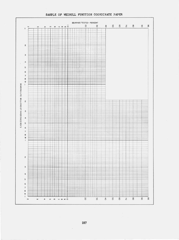
The five tables described above are followed b.\~ a specimell workslleet 7 with identifying information removed. A sample of ~Weibull-function .coordinate paper is also included. This coordi nate paper had been used for graphing the r esults of all t he individual endurance tests a nd these graphs had accompallied t ltO works lJ eets submit ted to the Statis tical Engineering L aboratory.

6 TJ1C estimates for Llo and Lso are given in millions of revo lu tions fo r an com pan ies except com pany D . 'l'he liie estimates [or D are shown in hours, tl1C same units in w hicJl the original endurance data were given.

i Bearings marked "Omitted" wore completely eliminated from conSidera tion, as company representatives expJained that these were non­fatigue failures and should not be regarded as part of the test grou p. As a result, the test group in the case of the speci men sheet shown was taken to consist of 23 bearings rather than the origirtal number of 25. 'J'b is type of s ituation appeared rather infrequen tl YJ however.

280

TABLE A- I. Sumnwl'y ball-bearing data for company A, with computed values for L IO, LSD, and W eibll11 slope e

Recor d Year Number Z Da e

No . of in test Load Number Ball diam. L L50 Weibull 10

t est gr oup of balls slope

Ib in .

1- 1 1936 24 4240 8 11/16 19.2 84.5 1. 27 1- 2 1937 20 4240 8 11/16 26. 2 74. 2 1.81 1- 3 1937 14 4240 8 11/ 16 11.1 68 .1 1.04 1- 4 1937 19 4240 8 11/16 11.8 66. 8 1.09 1- 5 1937 18 4240 8 11/16 13.5 79.4 1.06

1- 6 1938 21 2530 9 1/ 2 5. 80 25 .7 1.27 1- 7 1938 28 4240 8 11/16 18. 3 44 .7 2.10 1- 8 1938 27 4240 8 11/16 5.62 73.2 .73 1- 9 1940 20 4240 8 11/16 15. 8 82 .7 1.14 1-10 1940 22 4240 8 11/16 8.70 41 . 6 1.20

1-11 1940 19 4240 8 11/16 1l.6 160 .72 1-12 1940 15 1940 9 7/16 20. 6 71.4 1.52 1-13 1940 15 1940 9 7/16 14. 5 88. 2 1.04 1-14 1940 15 2536 9 1/2 12.1 33 .1 1.87 1-15 1940 14 2536 9 1/2 15.1 46 .4 1.67

1-16 1940 15 2536 9 1/2 14. 0 43 . 6 1.66 1-17 1940 14 2536 9 1/2 19.3 51.8 1.91 1-18 1940 26 4240 8 1l/16 46. 2 110 2.17 1-19 1940 14 4240 8 11/16 30. 0 88. 2 1. 74 1-20 1942 20 4240 8 1l/16 21.1 57 .4 1. 89

1-21 1942 20 4240 8 11/16 17.3 45 . 7 1.94 1-22 1942 37 4240 8 11/16 37 .5 118 1.64 1-23 1942 36 4240 8 11/16 20. 3 77 .1 1.41 1-24 1942 32 4240 8 11/16 4. 03 42 .5 . 80 1-25 1941 28 2544 8 17/32 8.38 84 . 7 . 81

1-26 1943 23 3975 8 19/32 1.79 13.5 . 93 1-27 1942 30 4400 10 5/ 8 11.7 45 .1 1.39 1-28 1942 31 6920 8 7/8 4.15 15 . 8 1.41 1-29 1943 30 990 9 5/16 7. 23 41 . 0 1. 09 1-30 1943 30 1509 7 7/16 22 . 9 110 1. 20

1-31 1943 30 932 7 11/32 9.54 31 . 6 1.57 1-32 1944 26 3180 8 19/32 6.28 23 .0 1.45 1-33 1944 29 3180 8 19/32 4. 81 21.2 1.27 1-34 1944 33 8640 10 7/8 4.17 12. 8 1.68 1-35 1944 26 14080 8 1-1/4 5. 42 31. 6 1.07

1-36 1951 28 1940 9 7/16 7.47 49 .5 1.00 1-37 1951 34 2330 9 7/16 4.80 21 .3 1.26 1-38 1951 27 1550 9 7/16 14. 8 78.4 1.13 1-39 1951 29 1165 9 7/16 84.9 460 1.11 1-40 1951 27 2910 9 7/16 3.40 16.5 1.19

1-41 1951 27 3880 9 7/16 1.24 3.23 1.97 1-42 1951 26 776 9 7/16 241 951 1.37 1-43 1951 30 19750 8 1-3/4 3.01 12.6 1.31 1-44 30 2112 8 11/16 89.1 486 1.11 1-45

~ 30 4224 8 11/16 15. 2 104 .98

Q)

1-46 ,~ 30 8448 8 11/16 2.04 10.2 1.17 1-47

tlD 30 2112 8 5/8 51.0 376 .94 1-48

.., 30 4224 8 5/8 5.26 58.8 .78 0

1-49 z 30 8448 8 5/8 . 883 4.94 1.09

1-50 1944 30 4224 8 11/16 14. 8 57. 4 1.39

281

T AB LE A- 2. Summary ball-bearing data for company B, with computed va!ues f aT L JO , £ 50, and W eibull slope e

Record Year Number Z Da e

No. of in test Load Number Ball diam. ~O L50 Weibull

test group of balls slope

Ib in.

2- l 1940 19 57.0 10 3/16 6.68 13.4 2.72 2- 2 1944 20 570 9 5/16 29.8 70.0 2.22 2- 3 1946 23 580 9 1/4 16.3 55.1 1.55 2- 4 1946 23 580 9 1/4 28.5 69.2 2.13 2- 5 1947 23 580 9 1/4 16.4 49.3 1.71

2- 6 1943 10 665 9 1/4 10.3 40.1 1.50 2- 7 1944 10 665 9 1/4 25 .7 46.4 3.19 2- 8 1942 19 580 10 1/4 9.55 39.6 1.32 2- 9 1946 33 620 10 1/4 17.9 62.1 1.51 2-10 1947 15 620 10 1/4 19.9 73.2 1.45

2-11 1947 31 620 10 1/4 12.9 50.4 1.39 2-12 1944 19 625 10 1/4 19.3 46.2 2.18 2-13 1941 17 720 10 1/4 11.1 23.3 2.54 2-14 1946 60 980 11 9/32 15.7 43.5 1.85 2-15 1947 32 980 11 9/32 11.2 38.1 1.54

2-16 1950 49 600 11 5/16 417 809 2.85 2-17 1949 60 600 11 5/16 216 709 1.58 2-18 1943 20 900 11 5/16 35.6 100 1.82 2-19 1946 67 1220 11 5/16 12.0 42.2 1.50 2-20 1947 34 1220 11 5/16 8.53 46.6 1.11

2-21 1940 20 1370 11 5/16 6.77 18.9 1.85 2-22 1950 60 1415 11 5/16 13.5 46.5 1.53 2-23 1950 60 2243 11 5/16 2.32 8.06 1.51 2-24 1942 20 720 12 5/16 36.7 141 1.40 2-25 1946 55 1300 12 5/16 19.0 57.2 1.71

2-26 1947 30 1300 12 5/16 19.5 60.6 1.67 2-27 1944 20 1650 14 11/32 17.0 74.4 1.37 2-28 1946 59 1760 14 11/32 20 . 9 53.7 2.00 2-29 1947 34 1760 14 11/32 9.56 40.7 1.30 2-30 1940 20 2010 13 13/32 5.49 33.3 1.05

2-31 1940 9 2010 13 13/32 1.39 44.0 .54 2-32 1944 19 2140 13 13/32 9.80 82.7 . 88 2-33 1943 11 2630 15 13/32 5.19 54.9 .80 2-34 1942 12 5900 14 19/32 6.36 17.5 1.86 2-35 1947 19 5900 14 19/32 3.68 22.1 1.05

2-36 1947 20 8070 14 23/32 8.34 23.6 1.81 2-37 1942 12 8075 14 23/32 6.78 36.4 1.12 2-38 1938 10 565 9 .210 9.27 18.4 2.75 2-39 1940 23 720 8 9/32 18.2 56.9 1.66 2-40 1940 24 720 8 9/32 22 .8 56.2 2.09

2-41 1940 25 720 8 9/32 3.99 15.6 1.38 2-42 1940 21 720 8 9/32 9.07 29.4 1.60 2-43 1940 25 720 8 9/32 7.14 28.5 1.36 2-44 1940 25 720 8 9/32 12.5 26.4 2.51 2-45 1941 25 720 8 9/32 18. 8 48.7 1.98

2-46 1941 23 720 8 9/32 21 .5 53 .2 2.08 2-47 1947 33 860 8 5/16 17.1 59.0 1.52 2-48 1948 8 860 8 5/16 15.2 87 . 6 1.08 2-49 1943 20 900 9 5/16 30.1 92.3 1.68 2-50 1944 18 900 9 5/16 15.0 47. 6 1.63

282

'fA TILE A~2. SU'/nnWTY ball-beal·ing data for company B , with compu ted values f01· L, o, L;o, and lVeib1l11 slope e- Conti nucd

Record Year Number Z Da e No. of in test Load Number Ball diam. ~O L50 Weibull

test group of balls slope

Ib in. 2-51 1945 27 940 9 5/16 17 .5 52 . 8 1.n 2-52 1947 34 940 9 5/16 14.4 65 . 6 1.2.4 2- 53 1938 10 1180 9 5/16 8. 76 22 .1 2.04 2-54 1945 30 1580 9 3/8 12 .1 43.3 1.47 2-55 1947 33 1580 9 3/8 17 . 2 64. 6 1.42

2-56 1948 8 1580 9 3/8 10.7 34.6 1.61 C.- 57 1945 31 2160 9 7/16 10. 9 37.6 1.52 2-58 1947 30 2160 9 7/16 12.7 53.7 1.30 2-59 1938 9 2200 9 7/16 3.73 43.5 .77 2- 60 1947 30 2480 9 7/16 16. 6 78.3 1.21

2- 61 1950 40 1340 9 15/ 32 180 275 4. 44 2- 62 1937 19 1660 10 7/16 85 . 2 234 1.86 2- 63 1941 19 1700 9 15/32 57.1 230 1.35 2-64 1939 24 2480 9 15/32 15. 7 55. 8 1.48 2-65 1939 25 2480 9 15/32 27 .1 97. 8 1.47

2-66 1939 23 2480 9 15/32 21.7 122 1.09 2-67 1939 28 2480 9 15/32 13. 2 42 .3 1.62 2- 68 1939 28 2480 9 15/32 35.8 145 1.35 2- 69 ;1. 939 20 2480 9 15/32 12. 7 34.7 1.87 2- 70 1944 20 2480 9 15/32 10.1 27.8 1.87

2-71 1945 20 2480 9 15/32 8. 83 34.3 1.39 2-72 1938 10 2480 9 15/32 16.5 60.3 1.45 2-73 1942 11 2480 9 15/32 17.9 65. 8 1.45 2-74 1943 10 2480 9 15/32 15. 7 63.1 1.35 2-75 1943 20 2480 9 15/32 10. 8 42 .1 1.38

2-76 1944 18 21.\80 9 15/32 14. 2 39. 9 1.83 2-77 194LI 18 2480 9 15/32 19.0 67 . 8 1.48 2- 78 1944 18 2480 9 15/32 16.3 57.7 1. 49 2-79 1944 20 2480 9 15/32 2. 93 18.0 1.04 2- 80 1944 20 2480 9 15/32 5.69 25 . 4 1.26

2-81 1944 28 2480 9 15/32 9.54 39.9 1.32 2-82 1944 22 2480 9 15/ 32 12.6 55.7 1.27 2-83 1941.\ 23 2480 9 15/32 5.10 37. 5 .94 2-84 1944 18 2480 9 15/32 16.0 53.7 1.56 2- 85 1944 20 2480 9 15/32 1.98 22.1 .78

2- 86 1945 20 2480 9 15/32 5.65 28.8 1.16 2- 87 1945 20 2480 9 15/32 12.8 43.6 1.58 2- 88 1945 20 2480 9 15/32 9. 84 32.3 1.59 2- 89 1945 20 2480 9 15/32 12.1 43.0 1.48 2- 90 1945 20 2480 9 15/32 5.48 40. 8 . 94

2- 91 1945 20 2480 9 15/32 6.64 25 .3 1.41 2- 92 1945 32 2480 9 15/32 13.9 4l.9 1.70 2- 93 1946 35 2480 9 15/32 9.02 45.4 1.17 2-94 1946 34 2480 9 15/32 11.0 49. 2 1.26

2-95 1947 31 2480 9 15/32 14.5 73.6 1.16

2-96 1944 9 2480 9 15/32 5. 91 37.2 1.02

2-97 1944 10 2480 9 15/32 18.1 40.5 2.33 2- 98 1945 10 2480 9 15/32 17 .1 53 .3 1.65

2-99 1945 10 2480 9 15/32 32 .6 61.8 2.95 2-100 1945 10 2480 9 15/32 24.1 66.2 1.87

40401)1- 56--1; 283

TABLE A- 2. Smnmary ball-bearing data JOT company B , with computed val1tes J OT L IO, L50, and W eibull slo pe e-Continued

Record Year Number Z D e a No. of in test Load Number

Ball diam. ~O L50 Weibull test group of balls slope

1b in. 2-101 1945 20 2480 9 15/32 36.1 71.6 2.75 2-102 1946 20 2480 9 15/32 63.3 104 3.82 2-103 1946 12 2480 9 15/32 14.4 59.0 1.33 2-104 1946 11 2480 9 15/32 15.1 92.9 1.04 2-105 1945 10 2480 9 15/32 18.8 39.4 2.55

2-106 1950 12 2480 9 15/32 5.63 34.7 1.04 2-107 1950 12 2480 9 15/32 7.23 34.5 1.21 2-108 1951 30 2480 9 15/32 16.7 71.8 1.29 2-109 1951 63 2480 9 15/32 26.5 90.3 1.54 2-110 1950 23 2480 9 15/32 8.35 49.1 1.06

2-111 1943 19 3250 9 15/32 3.79 9.30 2.1.0 2-112 1937 10 3470 10 7/16 9.05 36.6 1.35 2-113 1944 20 4000 9 15/32 2.98 7.35 2.08 2-114 1943 19 2300 10 15/32 22.5 73.4 1.59 2-115 1938 10 2730 10 15/32 3.82 31.7 .89

2-116 1946 22 2660 10 17/32 6.55 20.8 1.63 2-117 1944 20 2250 11 15/32 17.5 64.3 1.45 2-118 1943 16 2300 11 15/32 61.7 152 2.10 2-119 1945 48 2840 11 15/32 18.6 42.7 2.27 2-120 1947 28 2840 11 15/32 21.6 66.3 1.68

2-121 1947 8 2840 11 15/32 11.9 39.1 1.59 2-122 1948 8 2840 11 15/32 13.9 50.6 1.46 2-123 1943 19 3200 11 15/32 7.80 33.1. 1.30 2-124 1944 28 4000 11 15/32 3.55 13.9 1.38 2-125 1943 19 4000 11 15/32 9.40 23.4 2.06

2-126 1947 23 6350 11 11/16 4.76 22.7 1.21 2-127 1944 20 12000 11 1-1/16 3.23 9.86 1.69 2-128 1944 20 12000 11 1-1/16 2.62 9.52 1.46 2-129 1944 9 12700 8 1-1/2 7.89 39.7 1.17 2-130 1949 18 16500 11 1-1/16 4.93 20.4 1.33

2-131 1950 20 16500 11 1-1/16 6.26 16.2 1.98 2-132 1938 8 565 7 5/16 37.3 103 1.85 2-133 1944 20 900 7 5/16 14.0 38.6 1.86 2';'134 1938 10 1650 8 13/32 30.3 87.6 1.77 2-135 1944 20 2250 8 15/32 25.7 71.2 1.85

2-136 1943 20 2300 8 15/32 10.5 60.4 1.07 2-137 1944 19 3200 8 15/32 10.3 24.1 2.21 2-138 1944 19 4000 8 15/32 4.56 12.9 1.81 2-139 1937 10 1710 8 17/32 25.1 274 .79 2-140 1938 9 2360 8 17/32 48.8 264 1.12

2-141 1937 10 2680 8 17/32 7.53 €i). 7 .90 2-142 1937 11 3850 8 17/32 14.9 62.6 1.32 2-143 1947 21 7760 8 29/32 4.57 43.4 .84 2-144 1943 12 9550 8 1-1/16 3.90 40.7 .80 2-145 1947 21 9750 8 1-1/16 15.5 79.4 1.16

2-146 1948 16 11400 8 1-3/16 10.2 43.9 1.29 2.;.147 1948 20 11400 8 1-3/16 4.71 16.9 1.48 2-148 1947 18 11420 8 1-3/16 10.1 34.2 1.55

284

T ABLE A- 3. Summary ball-bearing data for com pany C, with computed values for £10, £ 50, and Weibull slope e

Record Year Number Z De. e

No. of in t est Load Number Ba.ll di am. LIO L50 Weibull test gr oup of ball s slope

I b in. 3- 1 1942 94 1580 7 9/16 16. 9 64. 8 1 . 40 3- 2 1949 29 790 7 9/16 211 729 1. 52 3- 3 1949 35 1185 7 9/16 74. 4 287 1.40 3- 4 1940 29 1600 9 1 / 2 9. 62 40.1 1 . 32 3- 5 1945 10 1600 8 15/32 11. 9 66. 3 1.10

3- 6 1943 9 2275 7 17/32 13. 8 58 . 0 1.31 3- 7 1946 13 2540 8 15/32 2. 38 11.3 1 . 21 3- 8 1946 12 2540 8 15/32 2. 38 11.5 1.19 3- 9 1949 12 1580 7 9/16 8. 75 62 . 2 0.96 3-10 1949 12 1580 7 9/16 25. 7 113 1. 27

3-11 1947 24 1600 9 1/2 14.5 113 0. 92 3-12 1949 12 610 8 5/16 26. 8 65. 6 2.10

T ABLE A- 4. Summary ball-bem·ing data for company D, with computed values for £ 10, £ 50, and Weibull slope e

Record Year Number Z Da.

No. of in test Load Number Ball diam. * L* LIO 50 t est gr oup of ball s

Ib i n . 4-1 1946 19 1750 9 7/16 159 963

4- 2 1951 34 1750 9 7/16 71 . 7 526

4- 3 1951 56 1750 9 7/16 113 582

* Life estimates are i n hours .

404091-56-4

T ABLE A- 5. Summary of test groups of ball-bearing data

Company

A ___________________________________ _ B ____ ________________________ ______ _ _

T ype B- L ___________________ __ __ _ _ T ype B- 2 _________________________ _ T ype B- 3 _____ ____________________ _

C ___________________________________ _ I> * _________________________________ _

T otal (all companies) _____________ _

Number of test T otal number of groups bearings in test

50 148

12 3

213

37 94 17

group

1,259 3, 289

291 109

4,948

*These data were not used in t he main analyses..

285

e

Wei bull slope

1.05

0. 94

1.15

SPECIM~ WORKSHEET

Reference No .~ __________ _ Bearing Mfg . by;--_________ _ Bearing Tested by:-;::.,--:-r ______ _ Date of Test_--.-.:8~. -..:::2c::.6 -.....:4:t:6"--_____ _ Bearing No. ___ ~~~~--------Lead'-:-____ ~5['~,O;-::R~.L:"'7-----Speed __ ~--~~20~C~O~r~·fP~.m~.,_-----Lubrication: Type Jet Oil

FrequencY-'7T~ ____ _ Ball No. and Dia . __ -<..9_='-lo;./..::4:;....1I ____ _ Contact Angle, __ ~ __ =07o ___ ~-,~_ Groove Radius: Inner Ring'O. __ ~5:::1",-.6,:,-%'70 __

Outer Ring, ___ 5 ... 3,-,-''='O%",-o __ Number of Rows,-::-::--'l=--_______ _ Bore ____ --'2~0~~~.--------O.D .~---~4~2~mm~.~;;;:;_::::::__:::;:::_;;;,--Lot Siz e' ____ ..!.2""5~ _ __'TO!:ak~e""n_e~n~2""3:...--__

Bearing temperature measured on outer ring at point of maximum load. ____ _ Material: Type _____________ __

Source Rockwe·~1~1~H7a-r~d~n-e-s-s-o~f~:----Inner Ring 63 .5 Outer Ri ng, ___ ~6L~LL. ____ _ Ball 5, _________________ __

Ball Failure:~~-~1~3~----~52~%~ Inner Ring Failure_.J5 _____ ~2~0~%c__ Outer Ring Failure __ l~ _____ ~4~% ___

Test life in 106 revolutions: Median ______ .....:6~8~.~ __ ----__ ---

Mean~-------~7~1~.------­B-IO,-::-:~------=:.2;;-9.'-;;;;-----

Slope of Curve, ____ ---'2""."'2""3 _______ _ Test No . let

3183 71

286

Brg. No .

16 10

5 19

9 11 15 12 20 18 13 1 ~

3 4 6

25 22 17

7 23 24 21 8

14

Table Ordered According to Endurance Life

Endurance Type of Mill. Revs. Failure Renarks

17.88 Ball 28 . 92 Ball 33.00 Ball 41.52 lo R. ~2 . 12 Ball 45 . 60 Ball 48 .48 Ball 51.84 B;.J.l 51.96 Ball

1Ht- I.R. 55 . 5 I.R. 67. 80 Ball e7.80 I,,'lsP9 b7 . GO T, ];i epE>

68 . 61;. Ball 68 . 64 L. Bore 68 .88 ~ Disc . 84 .12 Ball 93 .12 Ball 98 . 64 loR.

105 .12 I.R. 10 2 · 8~ --;.. Disc. 127 . 9-2 Ba ll 128.04 O.R. 173.40 ~ Disc .

to

'" ,. ~ :z

'" r::: ."

'" I ~ r r 0 :z If>

0 ."

:;; :z

'" '" '" ,. n

'" '" '" < vi

2

3

4

5

6

7

8

9

2

3

4

5

6

7

8

9

2

3

4

5

6

7

8

9

'"

~=

'"

SAMPLE OF WEI BULL FUNCTION COORDINATE PAPER

1-

I- I-

1==1'=

1-

BEARINGS TE5TED- PERCENT

rL

-=

1--1-+-',

U

·l,i~ . 1+

J

'" o

I -I -I-

1-"·

'" o

'=

I-

287

--

h

'" o

I-

I--

I -f--

.-

F= §

I--

I-I---I-I-l-

1= §

I-

<­o

_ .-

1- +--

'" o <­o

-+

: .-

'" o

--

-\--

'" o

'" o

~ i--

I-1-

'" o

I-

.... o

_.

-

1-

.... o

f--

i----

Q)

o

Q) o

-

-

-

<J) o

<J)

'"

-

=

-

-= -= -

-:-= -

1--=

'" o '" '"

5 . Appendix B. Evaluation of L IO, L50 , and Weibull Slope e, by Using O rder Statistics for Censored Data

This is a technical appendix that gives the mathematical basis for estimating, for each test group, the values of LIO and L5D for use in the regression analysis discussed in appendix C, and also the Weibull slope e.

5.1. Wei bull Distribution

a. Cha racteristics

As noted in the text, the basic assumption for estimating L IO , L50' and e for each test group was that the probability distribution of fatigue lives of individual bearings could be represented by a "Weibull distribution." 8 This means that the observed fatigue lives (number of revolu­tions) of all the bearings in a test group of, say, n bearings constitute a random sample of n independent observations from a distribution whose cumulative (from above) distribution function (hereafter denoted by cdf) is 9

S(L)= Prob {life '2.L}

=exp [-(Lla)·], (B1)

where a and e are the two parameters to be fitted. They are related to LIO a.nd L5D by eq (B2a) below. The function S(L) is also termed the "survivorship" function. This distribution is one of three limiting types to which the distribution of the smallest member of a sample, under general conditions, tends as the sample size is increased indefinitely. (Another type is dis­cussed in the following section.) This matter was first studied chiefly by Fisher and Tippett [5], and for this reason the type (B1) is sometimes referred to as Fisher-Tippett type III for smallest values.

There are both theoretical and practical reasons for choosing the Weibull distribution (B1) as the underlying probability distribution for fatigue life.

Theoretical. Here it is assumed that fatigue is an "extreme-value" phenomenon, related in some manner to the strength at the ·weakest point in the material under stress. The theo­retical reasoning that proceeds from this assumption is mentioned by a number of authors, and is given explicitly, for example, by Freudenthal and Gumbel in [6, p. 316 to 318J. It leads precisely to the form (B1) (see eq (2.9) in [6]). It is recognized that this statistical assumption has not received universal acceptance. This paper is, however, not concerned with the relative merits of various statistical theories of fatigue, but m erely with consequences of a reasonable choice from among them.

Practical. Application of the Weibull distribution received extensive attention by W . Weibull in [19], where he showed that a distribution of the general type (Bl) represented certain fatigue-life data quite satisfactorily. In addition, inspection of the special "Weibull" plots accompanying the worksheets suggests that many can be fitted satisfactorily by a straight line r epresenting a Weibull distribution, as explained below.

The manner in which these graphs are constructed is described by Weibull in [19J. A sample of Weibull-function coordinate paper used for this purpose is included in appendix A. The essence of the method is that eq (Bl) may be converted, by taking logarithms twice, into

e(ln L )-(e In a)=ln[ln(l /S)]' (B2)

where "In" denotes the natural logarithm (base denoted by E) and S=S(L). From eq (Bl) and the definitions of LIO and L5D , when L = L IO, S(L)=.90; and when L = L 50 , S(L) =.50. These values substituted in eq (B2) give

8 So named for W . Weibull (cf. [18J, p. 16 if. ) , who is considered to be one of the first to study it extensively. , The use of a continuous instead of discrete probability distribution will introduce no appreciable error.

288

e(ln LLO)-e (ln a) = ln[ln (1j. 90)]=-2.25037}

e(ln L50)-e (Jn a) = ln [ln (1/ .50)] = - O.36651, (B2a)

the values on the righ t-hand side being obtained from [17, table 2]. These are the relatioo­ships between the parameters a, e, L LO, and L 50 . The right-hand numerical values will later be denoted by Y.JO, Y. 50 , respectively. Equation (B2) may be written

ex-a' = y,

where

x=ln L, a' = e In a, y = ln[ln (l /S )]. (B3)

The variables x, y correspond to the two scales shown on the WC'ibull-function coordinate paper in appendix A. The variable x, with unrestricted values, corresponds to the horizontal scale "Bearing life," having a logarithmic scale. The variable y is represented through the per­centage surviving, S, or rather through the (vertical) scale for "bearings tested- percent" = percent failed 10= l - S = P , which can vary only between 0 and 1. This scale also has no n.­uniform graduations, given by the iterated logarithm in (B3) .

The Weibull distribution is thu s seen to be equivalent to a straight-line relationship, wi th "Weibull slope" e, between the logari thm of fatigue life and an associated quantity y depend­ing only on its relative rank when the fatigue lives arc ananged in ascending order. Thus, goodness of fit of the straight line (B3) is equivalent to goodness of fit of a Weibull distribu­tion to the fatigu e lives L of an individual test group . In. fact, one common method of s ta­tistical analysis of fatigue-life data (Freuden thal and Gumbel [6]) depends llpon the usc of the classical method of least squares for fitting this straigh t line. This method is, however, subject to certain limi tations described below. Instead, an alternative method, presented in the following sec tions, is preferred that fits the distribution of x= ln L directly by usc of order statistics.

h. Limitations of Fitting by Least Squares

In the classical method of least squares for fitting the s traight-line relationship (B3) to a test group of ball-bearing data, pairs of values (Xi, Yt), i = l , ... , n, arc required. The values of x= ln L arc obtailled from the given data. However , the variable y, m easured through the percentage failing, P = 1- S, presents difficulties. The problem of how to plot P is known as the problem of "plotting position."

It seems clear that the values, P i, of the plotted variable, P , must somehow be relaLccl to the rank order of the bearings as they fail. A natural choice is the percentage failillg: P -j/n, where f is the rank order of failure in a test group of n. This is not advisable for reasons dis­cussed at length by Gumbel in [9 , p. 14], where he advocates the plot ting position j / (n + 1).11 Other workers take different posit ions, and the question of plotting position must be regarded as st ill unsettled .

A second difficulty with the use of least squares is that as usually used it fails to take adequaLe accoun t of the number of items remaining intact ("l'unouts") in. th e incompleted tests. As a final point, it is to be noted that the successive plotted poinLs arc not independent, as they represent Lhe observed lives in increasing order. A correct usc of leasL squares pro­cedures would have to take into account all the intercorrclations, which is not done in the usual application of the "method of least squares." The method of order statist ics described in section :3 has the advantage of avoiding the above limi tations of the least squares method .

10 The symbol P as used here should not be con[used with the same symbol [or load used in the Ii[e [ormula. In any evcnt, the meaning will be clear from thc context.

11 This plotting position was also lIsed by Weibun in [1 8] (cf. eq (72) and the vertical scale in figures 3 and 4 thercin).

289

5.2. The Extreme-Value Distribution

a. Relation to Wei bull Distribution

The preceding section indicates that logarithms of lives, rather than lives themselves, are the natural units in which to carry out the analysis. This idea has also been adopted by those who do not use the Weibull distribution, either because they are unaware of its existence or because they do not feel it fits their data.

If the Weibull distribution is adopted for fatigue life, L, then the variate, x= In L, has the nonnormal cumulative distribution function 12

G(x) = Pro b {ln (life) ?': x } = Pro b {life ?': ~x}

This may be written G(x) = <P (y ) = exp ( - ~Y) ,

where

and u = ln a, (3 = l /e

(B5)

(B6)

(B7)

are the two parameters. The distribution, <I>(y) , considered as a distribution of the "reduced variable," y, has standardized parameters u = O, {3 = 1, and is called the "reduced distribution. "

The form (B5) is another of the three asymptotic distributions of extreme valu('s, some­times designated as Fisher-Tippett type I for small est values. This distribution has been studied extensively, chiefly by E. J . Gumbel (e. g., [7, S, 9]). In this paper, the term "extreme­value distr:bution" will be given to the distribution of smallest values (unless otherwise speci­fied), although this name is frequently given to the largest-values case.

From the above discussion, it is apparent that methods pertinent to the type I extreme­value distribu tion (B5) are appropriate. For this purpose there is available a mathematical approach recently developed by one of the authors of this report, and described in detail in [13].

b. Characteristics

A description of the extreme-value distribution (B5), together wi th an interpretation of its parameters in terms of life estimates (or rather their logarithms) , is essential to an understand­ing of the application of the method of order statistics in this paper. It will be seen that the problem of estimating life is equivalent to that of estimating the param eters u and (3.

The parameters of the extreme-value distribution (B 5) are depicted in figure 1 (page 291). The quantity u is the position of the mode or highest point of the (frequency) distribution. The quantity (3 is a scale parameter, analogous to the standard deviation, !J" , in the case of the normal distribu tion. In fact, {3 is -/6/7r (abou L %) times the standard deviation of the extreme­value distribution.

Although the two parameters, u, (3, completely specify the distribution, it is very useful to introduce related quantities of the form

(BS)

which are linear combinations of parameters u and {3 and may thus also be regarded as param­eters when known values are later assigned to y. Introduction of t makes it possible to esti­mate u and (3 simultaneously. Thus if t can be obtained as a+ by with u and b known and y arbitrary, then the values 1o= a, (3 = b can be read off at once.

The parameter t has another highly important meaning . In figure 1 the area F under the distribution to the right of the ordinate erected at t represents the probability that a value

" Cf. Freudenthal and Gumbel [6J , eq (2.5) , (2.6), (2.8), (2.9) .

290

-x

(!)

II -x

0' x,O=lnL IO=u+I3Y.90 z o ~ u z :::> lL

>­~

ff)

Z W o

Y.90= - 2.25037

x=ln L

FIG U RE 1. General form of extreme-value distribution (for smallest values) showing relationship of parameters tF) :lllO = ln L lO ) and x50 = ln L 50 ) to u and B.

291

larger than t will occur. Thus t is a function of F and may be written tF , as shown; it is desig­nated the "upper lOOF-percentage point" of the distribution. For example, if F = .90, then t= t.oo represents a value of x= ln L , which will be exceeded by 90 percent of the population. This is associated with rating life LlO (life exceeded by 90 percent of bearings) by the relation

(B9)

where x represents life in logarithmic units. Similarly, for median life,

(BlO)

Since the t's are regarded as parameters of the distribution, so also are XIO and Xso, and therefore LIO and L50 • These are not, of course, all independent .

In general, we have the percentage point tF , which, expressed in terms of the original param­eters u and fj, may be written in the form (B8):

where y is a quantity depending only on the probability F, determined as follows. We have from (BSa)

i. e., YF is the value of (x-u)jfj when x takes the value tF. But by definition of the probability F, in view of (B5), (B6), and (Bll),

(B12)

Thus, solving for YF, we obtain Yp = ln(-ln F). (B13)

This is the reduced variable corresponding to the probability F, and may be obtained by a simple change in sign from table 2 of [17], which tabulates the function

where <I>l" a probability, takes on values from ° to 1. Thus,

for F = .90, YF=-2.25037;} for F = .50, YF=-0.36651.

(B14)

The above discussion shows that both XIO and X50 (rating and median lives in logarithmic units) may be determined once the general percentage point (BSa) is estimated by giving the two particular values (B14) to YF.

c. Conversion From Largest to Smallest Values

The methods and numerical results developed in [13] were for problems, such as maximum gust-loads on airplanes, that required the distribution of largest sample values. In order to adapt this material to the distribution of smallest values (B5) required here, t he relationships of symmetry involved in the reversal of direction must be examined with care. To avoid confusion, it is necessary to use subscripts Land S to distinguish between quantities related to the largest-value distribution from those related to the smallest-values case. No generality is lost by use of reduced variates. Thus, in (B5), x will be replaced by the reduced variate y, and, for simplicity, the symbol G(y) will be used instead of <I>(y) :

G(y) = <I> (y) = exp( - EY).

292

(B15)

From this, the ("cumulative from above") distribution of smallest values is

- oo < y< oo, (B16)

where Ys denotes the reduced smallest value. The corresponding distribution of largest values is (sec Gumbel [9, eq (I ), p. 21])

Prob { Y L "2:.y} -= Ih (y) = l - Prob {YL< y } = I - exp( -e-V) = l - Gs ( -y), -00 < y< 00 ,

from (B1 6) .

(BI7)

The corresponding relation for the density functions is obtained by differentiation, with gs(y)= G~(y), and hL(y ) = Hf (y ):

H ence the two distributions arc merely mirror images of each other. The moments of the distributions are related as follows:

(BI9)

Thus, the means differ in sign and the variances arc identical:

(B20)

(B21)

These values arc given, for example, in [9, p. 23, eq (3.27)J. Finally , we need the relationships between moments of the order statistics for the two

distributions. As the smalles t-value distribution is a r eversal of the largest-value distribution, it is natural to reverse the arrangement of the order statistics as well. This gives simpler results. Thus we arc interested in the ith order statistic in the series

(8 ): y;"2:.y~"2:. ... "2:.y~"2:. ... "2:.y~, (B22)

where Lhe parent distribution is Lhat of smallest values. Primes will be used as a reminder that the order is descending, not ascending. Thus in tables B- 2 and B- 3 the absence of primes indicates that the order statisLics arc in increasing order.

(B22) is the analogue of the series

(L ): Yl ~Y2~ ... ~Y i ~ ... ~yn (B23)

of order statistics for the largest-value parent distribution. "Whenever a distinction is neces­sary the subscripts 8 or L will be used with the y's.

From (B18) it may seem intuitively (and may be justified rigorously) that the distribu­tions and moments of the order statistics follow the sam e symmetry relationships as the parent distributions, namely,

Es(y;m) = (- l )mEL Cy'[')

Es(y~y;)=ElJYiyj)

,2 _ 2 () 2() _ 2 US. i =US Yi = UL Yi =UL, i (B24)

In other words, the even moments remain the sam e; the odd moments change only in sign. The above development shows that the n umerical results for moments of order statistics

previously ob tained in [13J for the largest-valu e case can b e used here for smallest values without any substantive change.

404091- 5G- 5 293

5.3. Method of Order Statistics for Censored Samples

a. For Small Samples

Consider an independent random sample of n items from the distribution of smallest values, of which only the k smallest values can be observed. In view of the preceding dis­cussion, it is desirable in the theoretical development to deal with the order statistics in descend­ing order:

(B25)

where the parentheses denote the (n-k) (largest) unobservable values, and the remaining k values are known. This arrangement materially simplifies the exposition. Primes will again be used to denote descending order to distinguish from ascending order, which will occur in the later parts of this section .

From the k known values it is desired to determine an estimator

(B26)

(i. C., the weights w~) of the general parameter,

(B27)

of the extreme-value population CB5), such that T'in (B26) is (1) unbiased and (2 ) of minimum vanance. Mathematically, this means that

(B28)

where E denotes mathematical expectation, and

Val' (T') = a minimum, (B29)

subject to the above condition. From (B6),

(B30)

where y is the reduced variable and x the observed variable. From this the following relations for the order statistics Xi and Yi are apparent:

X~ =u+ f3y~, j = n - k + 1, n - k + 2, ... ,n, (B 3!)

CB32)

CB33)

(B34)

The values Es(Y~) may be obtained with the aid of the table in r14]. This table gives the values of EL(Y~) where the order statistics, y~ , are in descending order (as indicated by the prime). The means needed in (B34 ) are obtained from (B24) and the evident symmetry relations

as

Reference [14] gives the values of EL(Y~) for r= 1(1)min(n,26), n = 1(1)10(5)60(10)100. From CB28) and CB31),

k

E(T')= ~ w~ [u+f3ECY~_k+'j)] = tF= u +f3YF' j= l

294

CB 35)

(B36)

This is required to be an identity for all values of the parameters u , f3. Equating LiJeiJ' co­efficients gives the two conditions on the weigh ts , w~:

k k

~w~= l , ~ [E(Y;'_k+j)]W~=YF' (B37) j= l j=l

where the numerical ya.lues E(Y~_k+j) may be obtained from [14] as already indi cated. For thc variance condition (B29), we have , in view of (B26),

(B3 )

V ' (T')-[ '~ '2 , 2 + ,~ ""' " ](32_ T 7(n)' (3 Z at - ""W j (In-k+j "'''' W i W j (Jn-k+i,n-k+J - V k (B39)

= minimul11. subject Lo (B28).

Use of Lagrange mul tipliers in the same manner as in [13 , pp. 50- 52] gives, afLer difrerentiat ioTI, the conditions on the weights:

(B40)

For each fixed value of k :::;'n there are k l inear eq uaL ions which , wiLh Lhe Lwo in (B37 ), form a simultaneous system of (k + 2) equat ions in the (k + 2) unknowns, w~ , w~ , ... , w~, A, J.L. The value of A and J.L are u eful as a check, because, if (B40) is mulLipl.ied by Wj and summed for j = 1,2, . .. , k , the resul t is, in view of (B37) and (B39),

The minimum value, n:'~n' will be denoted by Q~,k' In general , there will be a set of (lc + 2) linear equations to solve for each k = 2, ... , n. (1) Case k =n. For lc = n, the matrix of coefficients and right-hand" constant terms" of

(B40) and (B37) is the (n+2) by (n+3) matrix , , ,

1 Ey~ 0 (Jll (J 12 (J I n

, , , 1 Ey; 0 (J21 (J 22 (J Zn

AO-n- (B42) , , ,

1 Ey.~ 0 (Jnl CT nZ (J nn

1 1 1 0 0 1

Ey; Ey~ Ey~ 0 0 YF

The ordinary (n+2) by (n+ 2) matrix of coefficients, without the constant terms, will be de-noted by An. If r " denotes the vector column of constant terms, then

A~= [A"i r n], (B43)

and the lineal' sysLem of (n+ 2) eq uations may be denoted

AnW;' = r n, (B44)

where W~ denotes the column vector of the (n + 2) unknowns w;, w~, . .. , w;" A, J.L.

295

1 __ _

The coefficients of the unknowns in (B44) involve the means E(y~) , already discussed, and covariances (]" ~ j . These values are given in table B-1 for n = 2 to 6. The (]"~j were computed by the method developed in [12]. Table B- 1 also indicates how the moments for the largest values case can be obtained simply from those shown.

The (n + 2) solu tions of (B44) are all expressible linearly in terms of the components of r n. Thus the solutions all take the form

A= c; + d;yp

J.I.= c~+d~yp

Substit uting these w~ in (B39) gives an expression of the form

O~.n= V~~~n=A~+2B~yp+ C~y~.

(B45)

(B46)

The quantities a~, b~ for the weights w~, for n = 2 to 6, are shown in table B- 2. The coeffici ents A~, B~ , C~ of O~. n, and the values of O~.n evaluated at F= .90, .50, corresponding to L Io, L oo. respectively, are given in table B-3.

Calculations were limited to n=6 in this paper , in view of the diminishing retmns in "efficiency" (see below) for increasingly larger amounts of computing. Methods suitable for larger values of n are discussed later.

Table B-3 shows that as sample size increases from n = 2 to 6 (in the case k = n ), the variance diminishes :for the percentage-point parameters tp for F= .90 and .50, i . e., tp= xlO= ln L IO and tp=x50= ln L oo. This is a common characteristic of the behavior of estimators for increasing sample size. Anoth er method whereby estimators may be compared is tbrough thei r efficiency.

Efficiency is a measme intended to provide a convenient standard of comparison for estimators. This is done for two estimators to be compared by dividing the variance of each into a theoretical "smallestJJ variance, OLB, known as the "Cramer-Rao lower bound." Further details in the case of complete samples where k = n, as here, may be found in [13 , p . 14 and 15]; values of OLB are also indicated in this r efer ence in table III (a).

T able B- 4 shows the effi ciency values so obtained , for the case k = n, n = 2 to 6, as regards the order-statisti cs estimators for the parameters xlO=ln L lO , xso= ln Lso.

These values show that for XIO, the effi ciency, starting with under 70 percent for n = 2, increases rapidly until 89 percent, out of a possible maximum 100 percent , is reached for n = 6. A 90-percent-efficient estimator is generally considered to be quite good . As regards XoO,

the efficiency is wen above 95 percent for all the values of n, and for n = 6 exceeds 99 percent. In view of results of this natme, and because of the increasingly heavy computations necessary, calculations were not carried beyond n=6 in [13] .

The above applies to estimation of the p aram eters XIO and X50, which it will be recalled are the logarithms of the actual life estimates L lO , Lso. It is believed that efficiency of the method of order statistics in obtaining estimates of actual life L lO , Loo is probably reasonable, in view of its high efficiency in estimating the logarithms, XIO, X50'

(2) Case k< n. For the case k<n, the procedure is very similar . One starts wi th a (k + 2) by (k+3) order matrix A2 derived from A~ in (B42) by striking out the first (n- k) rows and columns. One proceeds in this manner for k= T&- l , n-2, etc., until when k =2 the matrix becomes

I

(]" n - l. n-l

I

Un,n-l

1

I

(In-l, n

I

(J nn

Ey~

representing a set of 4 equations in 4 unknowns.

296

1 o

1 Ey~ o (B47)

o o

o o YF ,

The r esulting weights w; and variances Q~.k were obtained in similar Imanner to those for k = n in (B45) and (B46). These, it will be reealled , are primed quantities, associated wi th descending order of th e order statistics. Because th e observations, x, for surcessive failures naturally occlli' in ascending order, it is more useful for ac tual application, in contrast to theo­retical development, to tabulate the weigh ts and covari ances for the ord er statistics in ascending order. This has been done in table B- 2, giving the \.\Teigh ts w i= ai+ biyF', and in table B-3, giving the variances Qn,k=A+2ByF'+Cy~ for the estimators T n,k formed with the above weights. These varian ces arc also evaluated for the pa rameters :r1O= ln L 10 , :1'50= ln Lso. The relationships of these unprimed quantities to the primed ones of the previous theo retical development is merely a reversal of the ord er throughout, as ind icated by subscrip ts: i. e., every a~ is changed to the corresponding ak-i+1 and similarly for b ~ and w~. The vari ances Q m ay be shown to remain unchanged.

b. Extension to Larger Samples

Samples of more than six items arc broken up into independent samples of 6 with a re­mainder subgroup , if necessary, of from 2 to 5 items. Because the endurance data were arranged in increasing order of life, independent r andom subgroups could not be obtained by simply taking groups of 6 ill the (numerical) order in which they appeared on the worksheets. It was therefore first necessary to randomize the enclUl'ance lives on each data worksheet. This was accomplish ed by use of r andom numbers that were generated in the electronic computer (the SEAC) as needed.

Such al'tificialrandomization is no t desirable when it can be avoided, because the results of the calculations are then no t unique, but may depend to a limi ted degree on the particular set of random numbers used. 13 I t is therefore recommended that when the bearings in a test group are to be simultaneo usly nm on a battery of fatigue-testing machines, the individual bearings should be recorded in advance in some more or less natural order independent of the order in which failure takes place in the course of the test . K atural order migh t be order of manufacture, order of testing, etc.

In the present investigation, each subgroup was t reated as a random sample by the methods already developed for size 6 or less. That is, a "subes timalol' '' was calculated for each sub­group and the results averaged to produ ce an over-all sample estimator.

An es timator, botb for the individ ual subgroup and for the over-all sample, was obtained for each of the four populaLion quantities:

(B48)

For subgroups, these foul' parameter estimates are given by (caret denotes "estimate of")

(B49)

where Y .90= - 2.25037, Y.so= - 0.36651 , and Xl::; X2::; . . . ::; Xk, 2::; Ie::; n::; 6, arc the logarithms of the actual observed lives in a subgroup arranged in ascending order, and the ai and bi are read directly from table B- 2. For the over-all sample estimator, the subesLima tol's Tn, k are merely averaged.

For la ter usc (appendix C) the variance of the over-all estimalor, T, and its relat ion Lo sample size will be considered here. Consider first the case of a complete sample, where no intact bearings arc present because the test is run to completion. L et n be the sample size; then there arc two cases, according as (J) n ::;6, or (2) n>6.

13 Thls effect can bc reduccd somewhat by making a duplicate run and averaging the results, as was done in this study.

297

10 ,..------"""T""-----,--.----,-.,...---,--,-~ 1.0

9 ~

.8

.7

6

4

0'0 (SCALE AT LEFT)

3

0.0 (SCALE AT RIGHT!

4 6 7 8 9 10

.6

.5

.4

.2

.1

FIGURE 2. Relationship of variances QlO and Qso to sample size n for n = 2 to 6 (logarithmic scale in each direction) .

£110 is variance of estimator of xJo=ln LIn Qso is variance of estimator of x6o= ln Lr.o

All Q's are ill units of {J2

(1) n~6. Table B- 3 gives the numerical variances, QIO and Q50, for n = 2 to 6. These values are plotted in figure 2 on double-logarithmic paper. The values for Qso (right-hand scale) are seen to lie on a straight line of slope negative unity. This shows that at least in this case, variance is inversely proportional to sample size. For the other case, QIO, a straight line also gives a reasonably good fit, and its slope appears to differ only a little from - 1. Hence the underlined statement is approximately applicable here too.

(2) n > 6. If a sample of size n > 6 is broken into equal subgroups (of size 6, for example) ther e will generally be a remainder of size less than 6. The preceding development, when suitably modified, shows that for large n the influence of this remainder is small compared to the remaining bulk of the sample and thus the rule in question holds approximately in this case. Agreement with the rule is less close for a few cases of moderate n, but for simplicity the inverse relationship will be taken as a reasonable rule of thumb in all cases for the over-all purposes of analysis.

Two complete runs were made on the SEAO for each of the 213 test groups of data, and the two results were averaged for each group, giving values of the averages

(B50)

From these, the values of LIO and Lso were obtained from a table of exponential s and the Weibull slope e= l !fJ obtained as a consequence of formula (B5). An example showing the steps in calculation of L IO , L so , and e is discussed below.

Because this investigation represents probably the most extensive mass fitting of the Weibull distribution made to date, a tabulation of the 213 values of the parameter e will be of considerable value to future applications of this distribution. This is shown in table B- 6. The corresponding histogram is given in figure 3. Particular items of interest are

mean of e (all 4 companies) = 1.51,

median e (all 4 companies) = 1.43.

Note that 50 percent of the values are in the interval e= 1.17 to 1.74.

298

-- ------

70 r-.---,_--_.--~----r_--,_--_.--~----r_--._--_r--_.--_,r_--._--_r--_.--_._.

6 0

Vl 50 IlJ If) <t U 40 u. o

~ 30 !Il :::!! :::> z 20

10

. 50 1.00

Z <t o w ::i!

1.50 2 .00 2.50 3.00 CLASS INTERVALS FOR e

3.50 4 .00 4 .50

FIGURE 3. Histogram for the 213 estimates of parameter e for companies A, B, C, and D combined. Data i ll table B-fl

c . W oIked Example

The example that will be given 1,0 illustrate the foregoing proeedures will be t he one that was worked out as a "test problem" for (,he SEAC before using the full set of da ta. The test group of bearings selected for this purpose was No. 1- 1 in table A- I , for company A. The test group consisted of 24 ball bearings, of which 4 remained intact when the test was discontinued. The details of the computation for obtaining values of LIQ, L5o, and 'iV eibull slope e from the test group of data are contained in Lable B- 5 and described in the steps below.

The endmance lives in observed (increasing) order are lis ted in eolumn (1). The arrows indicate the four "run-outs," or "intacts," whose testing was diseontinued at the number of million revolutions indieated. All th at is known about these foUl" bearings is th at their fatigue lives exceeded the values shown.

Stez) 1. Randomization . The order of endmance lives in column (1) was randomized by use of a se t of random numbers generated in the SEAC as part of the computation work. Tho r esult is shown in column (2) of table B- 5.

Step 2. Subgroups . Tho lives iurandomized order were divided , as shown by the linos of separation, into subgroups of size n = 6, the maximum size for which tho order-statistics weigh ts had been computed .14 Each subgroup was then prepared for the application of tho order­statistics method by rearranging in increasing order (column (3)). N atmallogarithms wore then taken as in column (4) .

S tep 3. W 6ights. Each subgroup was regarded as consisting of k actual obser vations out of a censored sample of n. It h appened here that n was 6 for every subgroup; k took the values 6,5 , 6, :3 . These values are shown in the subscripts of T n. k written in col umn (3), and they determin ed the weights ai and bt to be selected fmm table B- 2. These weights are represented in columns (5) and (6).

Step 4. Gross-products. The cross-products

wer e then evaluated and placed as shown for each of the subgroups.

II As sample size 24 is an exact multiple 01 n=6. it so happened that therc was no "remainder subgroup" in this case. This will not usually be true. but tbe procedure is identical 101' other valucs 01 n, differing merely in the numerical weights to be used.

299

Step 5. Estimates. A simple arithmetic average of the four values was taken for each of - A - A

the two columns (5) and (6), and denotcd by T1 = u, T 2 = (3, respectively. These are the order-statistics estimates of the two parameters u and (3 of the extreme-value distribution that represents the underlying Weibull distribution.

The reciprocal of ~ yields the Wei bull slope e = 1.32497. (A) The following logarithmic life estimates were given by following linear combinations of

the estimates u and ~, using the given values of Y .90, Y .50: A A

xlO = ln LIO= u - 2.25037 (3 = 2.982305 A A

x50 = ln L 50=u-0.36651 (3 = 4.404120

rating life LlO= antilog (XlO) (base ~) = I9 .2333 million rev

median life L50= antilog (X50) (base ~) = 81.7872 million rev.

(B )

(C)

These three values (A), (B), and (C) reprcsent the outcome of the calculation. In the full-scale computing program, calculations were carried out by the SEAC to a larger

number of places than is shown in the table for presentation purposes. In general, however, the number of places shown here should be adequate. The values L lO , L50, and e shown here differ slightly from those recorded in table A- I because the latter represent averages of two separate runs.

TABLE B- 1. Means, variances, and covariances of order statistics Yi in samples of n from the reduced extTeme­value distribution G(y) = exp(-cy ), n = 2 to 6

Means* n i Es(y:)

=- EL(Yi)

--

2 { 1 O. 11593 152 2 - 1. 27036 285

r 1 O. 40361 359 3 1 2 - .45943 263

3 - 1. 67582 795

1 1 O. 57351 263

4 2 - .10608 352 3 -. 81278 175 4 - 1. 96351 003

\ 1 O. 69016 715 2 . 10689 454

5 3 - .42555 061 4 - 1. 07093 582 5 - 2. 18665 358

1

1 O. 77729 368 2 .25453 448

6 3 - .18838 534 4 - .66271 588 5 - 1. 27504 579 6 - 2. 36897 513

For distribution of largest values, Vl~V2~ •.• ~Yn For distribution of smallest values, v;::::y;:::: ..• ::::v~

Variances and covarianccs,* U:i= U:i= Uij= U ji

j = 1 j = 2 j = 3 j = 4 j = 5

O. 68402 804 O. 48045 301 1. 64493 407

.44849 796 O. 30137 144 0. 24375 810 .65852 235 .54629 438

1. 64493 407

.34402 417 .22455 344 O. 17903 454 O. 15388 918 .41553 113 .33720 966 .29271 188

· 65180 236 .57432 356 1. 64493 407

.28486 447 . 18202 536 · 14358 737 O. 12257 865 O. 10901 329 .30849 748 .24676 731 .21226 644 · 18967 383

.40598 292 .35267 072 .31716 095 · 64907 319 · 58991 519

1. 64493 407

.24658 20 . 15496 74 · 12121 61 · 10291 64 0.09116 19 .24854 56 · 19670 62 · 16806 28 · 14945 32

.29761 59 · 25616 60 .22887 90 .40185 52 · 36145 55

· 64769 96

1

j = 6

O. 08285 42 . 13619 10 . 20925 46 .33204 51 .59985 67

1. 64493 41

*The means are for smallest values (denoted by subscript S) ; for largest values, change all signs and reverse order of y's . The U ij are the same for both.

300

TABLE B- 2. W eights Wi for the order-statistics estimator T n. k for the param eter tF = u+ {3YF oj the extreme-val ue distribution (sm allest values) from a censored sample of n = 2 to 6, where only the k smallest vallbes are known

Tn .• =w,x,+w"",+ ... +w.x"wj=aj+bj!lp

x,:S;x,:s; . .. :S;x.,k=2ton

,-- I

n k I - --

Xl

I X2 X3

I X,

I

X5 Xo

2 2 {ai 0. 0836269 O. 9163731 bi - . 72 13475 · 72 13475

{ 2 {Cti -. 377700 1 1. 3777001

3 bi - . 8221012 O. 8221012

3 {Cti .0879664 · 2557 135 O. 6563201 bi - .3747251 - .2558160 . 630Mll

{ : {ai - . 7063 194 1. 7063194 bi - . 8690149 O. 8690149

4 {Ct . - .080 1057 .0604316 1.019674l bi - . 4143997 - . 3258576 0.7,102573

{Cti .0713800 · 1536799 .2639426 O. 5109975 bi - . 2487965 - . 2239 192 - .0859035 · 5586192

t {Cti - .9598627 L 9598627

bi - .8962840 0.89628'10 {ai - .210 1.1 41 - .0860231 1. 296]372

5 bi - .4343419 - . :3642463 O. 7985882 {Cti - . 0153832 · 05 1 96~2 · 1520750 · 8113<140

bi - .2730342 - . 2499429 - .149 J094- .6720865 {Cti . 0583502 · 10882:36 · J 676091 .2462831 0.4 1893-11

I bi - . J844826 - . 18J6564 - . ]304534 - . 0065354 .5031278

2 {Cti - 1. 1655650 2. J655650 bi - 0.9l41358 O. 9141358

3 {ai - . :3 153968 - . 20:3431.5 1. 5188283 bi - . -1~660 1 8 - . :3886492 0.8352510

6 4 {Cti - .0865:378 - .02805:34- .06-19390 L 0496521 bi - . 2858647 -. 2654739 - . 1858756 0. 7372142

5 {Cti . 00573U . 0465729 · 1002523 · 1722784 .6751653 bi - . 2015·1:31 - . 1972753 - . 1536040 - .0645894 .6170118

6 {Cti .0488669 · 0835221 · 1210527 · 1656192 .2254909 O. 355,1..J.sl bi - . 1+58072 -. 1495332 - . 1267277 - .073]937 . 0359868 .4592751

301

TABLE B-3. Variance Qn ,kfJ2 of order-statistics estimator T n,k, given in table B- 2, and its numerical valttes Qn,k(10)=QIO, Qn.k(50)=Q50jor estimators oj parameters t .90 = xlO = lnLIO, t.50 = x50 = lnL50, respectively, for a censored sample of n= 2 to 6

n I k A

- - ----- ---

2 2 O. 6595467

3 { 2 · 9160386 3 .4028637

{ 2 1. 3340189

4 3 O. 4331573 4 .2934587

1 2 1. 7891720

5 3 O. 5293953 4 · 2918142 5 · 2313953

{i 2. 2440055 O. 6529409

6 .3237 185 . 2236063 . 1911738

Variances in uni ts of {32

Cin,,=A+2BYF+ CyP'<

x,:S;x, :s; .•• ::;Xk, k=2 to n

B C --- ---------

0.0643216 0.7118574

.4682465 .8183654 - .0247719 .3447 117

.7720298 .8670220

.1180273 .3922328 - .0346903 . 2252828

1. 0115594 .8950462 O. 2353740 · 4168155 .0385708 · 2537913

- . 0339905 · 1666472

1. 2082248 · 9132926 O. 3332488 .4321160 . 1020223 .2697162 . 0105329 · 1861069

- . 0313731 · 1319601

010 0 50

------ - -----

3. 975015 O. 708021

2. 952920 .682735 2. 260033 .467327

2. 250056 .884572 l. 888278 .399329 l. 590460 · 349150

1. 769068 1. 167910 1. 580861 O. 412852 1. 403'158 .297633 1. 228307 .278697

1. 431164 1. 481035 1. 341381 O. 466709 1. 230430 · 285165 1. 118677 .240885 1. 000644 · 231897

<For QIO'YF = -2.250~7; [or O",Yp = -O.36651.

TABLE B- 4. Efficiency of order-statistics es­timator of logarithmic life xlO = ln LIO and x50 = ln L 50 for complete samples (k = n) oj size n = 2 to 6

n

2 3 4 5 6

E fficiency (in percent) with respect to

xlO = ln L lO

67. 2 78. 8 84. 0 87. 0 89. 0

302

X50 = In L50

97.4 98.3 98. 7 98.9 99. 1

---------

TABLE B- 5. Example showing use of order statistics method of computing values of L IO, L50, and e f rom endw'ance data

Test group 1- 1, company A

2 3 4 5 6

Endurance (mi ll ion revolutions) Weights

Observed order

6. 0

8. 6

17. 8

18. 0

27.5

33.5

50. 5

51. 5

69. 0

74. 0

74. 0

89. 0

109. 0

118.0

119. 0

138. 0

141. 0

144.0

146. 0

(150.0) ->

151. 0 ( 153. 0 ) ->

( 153. 0)->

( 153. 0)->

Natural loga-Randomized Ascending rithms Xi

order order within subgroups

119.0 27. 5 xl = 3.31419

138.0 69. 0 x2 = 4. 23411

146. 0 119.0 x3= 4. 77912

151. 0 138.0 x. = 4. 92725

27. 5 146. 0 x5= 4. 98361

69. 0 151. 0 xo = 5.01728

T o,o - __ ___ ---- -- ----- -

(150. 0)-> 6.0 x l= 1.79176

8. 6 8. 6 x2= 2.15176

51. 5 51. 5 x3= 3.94158

89. 0 89. 0 x. = 4. 48864

109. 0 109.0 x5= 4.61935

6. 0 ( 150.0 )-> (xo)

------ T 6 ,5 - - - - - - - - - - - - - - - - - - - - - -

74. 0 18.0 I x1= 2.89037

181. 0 33. 5 x2 = 3.5U55

141. 0 74. 0 x3= 4.30407

18. 0 118.0 x,= 4.77068

33. 5 141. 0 x5= 4. \H876

144. 0 144.0 I

xo = 4. 96981.

T o.o - - - - - - - - - - - - - - - - - - --

17. 8 17.8 I x1 = 2.87920

( 153. 0)-> 50. 5 x2 = 3. 92197

(153. 0)-> 74.0 x3= 4.30407

(153.0) -> (153.0 )-> (x ,)

50. 5 (153.0 )-> (X5)

74. 0 ( 153. 0 )-> (xo)

T6 ,3 - - - - - - - - - - - - - - - - - - - -

ai

0.048867 - 0. 145807

.083522 - . 149533

· 121053 -. 126728

· 165619 - .073194

.225'191 . 035987

.355448 .459275 k k

1:a iXi =LJ. 8173 10 1:&iX;= O. 400992 1 1

0.005731 - 0,201543

. 046573 -. 197275

· 100252 - . 153604

· ] 72278 - .064589

.675165 . 617012

--------- -- - - -- -- --------------k k.

1:aixi= LJ. 446363 1:b,Xi= 1. 2] 3655 1

I

1

[ Weights are same as] for first, subgroup

k k 1:aix;= 4.628081 1:b;x;= O. 619440 1 1

- 0.3 15397 - 0.446602

- .203432 -. 388649

1. 518828 .835251

---------- -- -- -- ----------------

-------- -------- ----------------

---------------- ----------------k. k.

1: aiXi= 4.831197 1:b;x;= O. 784853 1 1

O\'er-all estimator _____ ________ _______________ _____ 1\ = 4. 680738 1',=0. 754735

T ,= u = 4.680738

SUMMARY

T2=~= 0. 754735 e= 1/~= 1. 324 97

V .90 = - 2.25037 Y .50= - 0.36651

£1O= ln L IO =u+ V.90t3= 2.982305, LIO= 19.7333

£50= ln L 5o =u+Y .50t3= 4.404120, L50 = 81.7872

303

TABLE B- 6. Tabulation of estimated values of Weibull slopes, e,for the 213 test groups of companies A, B, C, and D

Company

Weibull slope, e A B C D

Total

- -------- -----------------------------------------

0.50 to 0.74 ________ _ .75 to .99 __________ _

1.00 to 1.24 ________ _ 1.25 to 1.49 _______ _ _ 1. 50 to 1. 74 ________ _ 1. 7 5 to 1. 99 ________ _

2.00 to 2.24 ________ _ 2.25 to 2.49 ________ _ 2.50 to 2.74 ______ __ _ 2.75 to 2.99 ________ _

3.00 to 3.24 ________ _ 3.25 to 3.49 ________ _ 3.50 to 3.94 ________ _ 3.75 to 3.99 ________ _

4.00 to 4.26 _________ _ 4.25 to 4.49 ________ _

TotaL _________ _

~ean ______________ _ ~edian ____________ _ 50 % interval * ______ _

2 6

16 11

7 6

2

-------50

1. 33 1. 27

1. 07 to 1. 59

*Firs t quartile to third quartile.

1 11

22 40 32 17

12 2 4 4

1

1

1

148

1.60 1.49

1. 27 to 1. 82

2

3 5 1

1

12

l. 31 l. 30

1. 08 to l. 45

1

2

3

1. 04 1. 06

0. 94 to 1. 16

3 20

43 56 40 23

15 2 4 4

1

1

1

213

1. 51 1. 43

1. 17to 1.74

6. Appendix C. Evaluation and Analysis of the Unknown Parameters in the Life Equation with Respect to Companies and Bearing Types

6.1. Summary

Equation (2a) of the main text,

expresses the dependence of fatigue-life L on the design characteristics of the deep-groove bearing (Z, Da), the bearing load P, and the "workmanship factor" fe. This appendix out­lines the statistical methods that were used (a) to determine "best" empirical values for the parameters jc, ai, a2, and p of this life jormula, (b) to derive the associated intervals of uncer­tainty, and (c) to answer various questions about the values of these parameters, from the basic endurance data furnished by the ASA Subcommittee, which are summarized in appen­dix A. These methods are applied separately in each case to the rating life LID and m edian life L 5D values derived from the endurance test data as described in appendix B.

Section 6.2 summarizes the application of the statistical methods used to determine best empirical values and intervals of uncertainty for the parameters jc, ai, az, and p in the case of deep-groove bearings. Sections 6.3 to 6.6 outline the statistical analyses employed to answer various questions about the values of je, ai, a2, and p for the ball bearings of companies A, B, and C. In particular, section 6.3 gives the analysis employed to determine whether values of these four parameters are the same for the bearings of the three companies . This analysis is carried out separately for rating life LIO and median life L 5D , and the postulated "complete between-companies homogeneity" is not supported in either instance. Section 6.4 gives the analysis appropriate to determining whether the data are consistent with the supposition that the value of p is the same for the three companies (regardless how the values of the other

304

parameters may differ); this analysis is applied to the L IO and L50 data, with an affirmative conclusion in both instances. It is concluded further that the data are consistent with the supposition that this common value for p is equal to 3.

Section 6.5 presents the analysis employed to determine whether the values of the param­eters i e, aI, az, and p are the same for the three types of deep-groove bearings (B-1, B-2, and B - 3) for which the data from company B were available. A negative conclusion is rcached. These data are then reanalyzed to determin e whether they are consistent with thc supposi­tion that p=3 for each of the three types, regardless of differences in the other parameters. An affirmative conclusion is reached in this case.

Section 6.6 concerns (a) the extent to which the L IO and L50 values are consistent with the supposition that the values of aI, a2, and pare 2/3 , l.8, and 3, respectively, as given in [15]; and (b), the determination of more precise values for fe in those cases in which thc foregoing supposition is supported.

6 .2 . Determination of " Best" Values for the Parameters a nd Their Associated Intervals of Uncertainty

As shown in section 2.2 of the main text, if natural logarithms are taken of bo tll sides of the life equation (eq (2a», th e resul ting cquation expresses the logarithm of rating life LIO (or median life L 5o) as a linear function of the logarithms of the characteristics of the bearing (Z,D a), and the bearing load P, with coefficients that are simple functions of the " workmanship factor" je and the exponents, ar, a2, and p; i. C.,

(01)

where

Y= ln L

(02)

x3=ln P

and

bo= p In fe=pao 1

(03)

are unlmown constants to be estimated from the data. The variables Xl, Xz, and X3 are fixed variates. Their valu es are uniquely determilled by

the design of the bearing and the bearing loads that are used in the tests. The variable Y, on the other hand, denotes the mean values of In L lo, or In L bfh for the population of all bearings with characteristics Xl and X2, tested at load X3.

In the practical situation Y is never known, but must bc determined from the results of endurance tests. The methods used for obtaining such estimates of Y from endurance-test data are given in appendi.x B. ero distinguish Y from an empirical estimate of it, the estimate will be denoted by the lower-case letter y.

Generally speaking, an estimate y is a random variable, having a probability distribution that depends on Xl, X2, and X3. We assume that the mean of this distribution is Y=Y (Xl, Xz, X3),

and that its dispersion, or more precisely, its va7'iance, is inversely proportional to the r umber of bearings w in the test group from which the estimate Y=Y (Xl' X2, X; w) is derived (cf.

305

L

appendix B) ; that is,

meanofy= Y } .J (r

variance of y= w' (04)

where 0- 2 denotes some positive cor stant , and w is the number of bearings in the test group. The statistical methods used to estimate the unknown parameters bo, bl , b2 , and 63 from the

data are termed regression techniques. The books by Anderson and Bancroft [1], Dixon and Massey [3], Hald [10], Kempthorne [11], Mood [16], and Will;:s [20] give extensive discussion of these techniques. For completeness, some of the techniques and rationale of regression analysis bearing on the work embodied in this report are summarized below. More detailed discussions can be found in the above references.

Estimation. The problem of estimating the unknown parameters in the life equation can be stated as follows: Given independent observations (y,,; Xl", Xz", X3"; w"') from n test groups (a = l,2, . .. , n) where y'" is the estimate of In LlO or In L 50 , Xl"" X2", are the logarithms of the bearing characteristics Z and Da, X3" is the logarithm of the load, and Wa is the number of individual bearings tested for the ath test group; required to estimate the values of the param­eters bo, bl , b2, and b3, in eq (01) using some optimum method of estimation.

Estimates for the bi (i= O,I ,2,3) that are free of systematic error and have smaller variances than any other linear unbiased estimates are obtained by minimizing the quadratic form,

n Q= ~ w",(y",-bo-blXl",- bZX2"- b3x3,,,)2, (OS)

0'=1

with respect to each of the bi (i= 0,l,2,3) . The resulting normal equations defining the parameter estimates can be written in the

form, 15

where

and Xo",= 1 for all a.

A A A A "'\

aoObO+ aOlbl+ao2b2+ a03b3=go A A A A

alObo+anbl + a12b2+a13b3= gl A A A A

a20 bO+ a21bl + a22b2+ a23b3= g2 A A A A

a30 bO+ a3l bl + a32 b2+a33b3= g3,

n ai)= ~W",Xi",Xj",

",=1

n

gt= ~ waxi"y'" a=1

i,j,=0,1,2,3.

i=0,l,2,3.

If one defines the residual sum of squares by

which also can be wTitten in the alternative form

then the optimum estimate of (12 is

(06)

(07)

(08)

(09)

(010)

"A caret ( A) is used here to distinguish the fact tnat the solutions of the normal equations are estimated values of the parameters and not the parameters themselves.

306

The quantity (n-4) is the rank of the quadratic form S, and is termed the degrees oj jreedom associated with S .

The above method of estimation does not depend on yO'. having a particular assumed probability distribution. All that is necessary to specify abou t the probability distribution of yO'. is that it possess a finite mcan fI,nd variance. The solu tion of the normal equations (C6) has the property that Lhe weighted sum. of squares of the deviations about y O'. will be a minimum. This is a so-called " least-square" property of the solu tions, but it is onl~~ a consequence of Lhe method and is no t the justification for usi.ng til lS method of estimation . The justification for Lhe method is LhaL this is the onl~T one that results ill minimum variance unbiased estimates for Lhe bi (i= O, 1, 2,3).

Values for bi (i= O, 1,2,3) , and hence for a i and p, can be obtained b~T using either the In L lo 01' In L so values for YO'.' J n all cases where the a i and p have been obLained for rating life L IO , ano ther set of parameters have also been calculated fOT median life L so .

lntel'vals oj uncertainty and injerences. The methods so far disc Llssed for finding estimates of unknown parameters need no assumption as to the form of thc und erlying probabilit.\T dis­tribu tion of YO'. ' However , something more must be assumed about the distribu tion of YO'. if (a) olle wishes to place an interval abo ut an estimate of a parameter that will include the "true" (or pOPlilation) value of the parameter with given assurance, or (b) if one desires to make inferences abouL the parameters of the life equa tion for the populaLion from which the bearings arc a sample.

Although the end urance lives for individual bearings may follow a \ iV eibull distribu t ion, the distribution of YO'. will not be of this form. However, the eslimate YO'. (of. appendix B ) is an average of several independent estimates, each based on linear function s of six or less order statistics. Hence, by the central limit theorem, the distribu tion of t he estimate YO'. will be approximated by a normal distribution when n is large (d. Cramer [2, p. 213]). The statistical tests of significance used in this report are not greatly afl'ected by moderate departures from normality. Therefore, for making all inferences, i t will be fur ther assumed that the estimates YO'. follow a normal d istribu tion.

The intervals of uncertainty calculated for each parameter are 95-pereent co nfidence limits (equivalcnt to the usual "two-sigma" limi ts), which were referred to in the main text . Confidence limi ts for the parameter p = - b3 can be calculated by using conventional meLhods. However the confidence limi ts for ao , ai, and az are somewhat more complicated. The method used here, for this purpose, is sometimes referred to as Fieller's theorem (cf. Fidler [4]).

In order to make inferences abo ut the parameters wiLh respect to the differcnt companies or bearing types, certain statistical tests of significance were used in this paper. 'l'hese are all based on a test statistic F, termed the variance ratio or F-ratio, which takes the form

where QI and Q2 ar e quadratic forms calculated from the data and VI, Vz are the respective ranl~s of the quadratic forms. The explicit expressions for Q! and Qz depend upon the particular hypothesis being tested. The subsequent sections that employ a variance-ratio statistic also give the explicit expressions fot' the two quadratic forms.

If the hypothesis being tested is true, then the calculated variance ratio will deviate from unity in accordance with its tabulated distribution. However, if the hypothesis is false, then the variance ratio will be substantially greater than unity, and the" more false" the stated hypothesis, the larger the value for the variance ratio. Thus when the hypothesis tested is false, this will be detected by an abnormally large F -ratio. In order to objectively determine whether a calcula ted variance ratio is significantly greater th an unity, one selects from tables of the variance-ratio distribution a critical value of F, such that there is only a small probability of the calculated variance ratio exceeding the cri tical value from purely chance causes. The critical value for F used for all variance-ratio tests , in tbis paper , has been selected so that there

307

is only a probability of .05 of i ts being exceeded by a calculated variance ratio from purely chance causes. This critical value will be denoted by F .05 (1I1,V2 ) ' More extensive discussions of these procedures are given in K empthorne [11, chap. 5] .

All statistical tests of significance to test relevant hypotheses h ave been carried out both for rating life L 10 and median life L 5o•

6.3. Analysis to Determine Whether Companies Have Common Values for All the Parameters

in the Life Equation

This section deals with t he details of estimating the values of the parameters in the life equation for each company. Furthermore, a statistical analysis is made to determine whether the companies have common values for all the parameters in the life equation. The F -ratio (eq (C16 )), which is used to test this hypothesis, is ob tained from the following procedures: A single set of parameters, bi (i= O, 1,2,3), is obtained by first fit ting all the data, irrespective of company, to the logarithmic life equation, and then calculating the resulting r esidual sums of squares 8 (eq (C14)) having 206 degrees of freedom. If the hypothesis of common values for all the parameters is not true, then a better fit to the data can b e made by fitting the life equation separately to each company. These calculations result in the individual residual sums of squares 8 1, 82, and 8 3 (eq (C13) ) having 46, 144, and 8 degrees of freedom, respectively. Thus the total residual sums of squares (8, + 8 2+8 3 ) will have 46 + 144 + 8 = 198 degrees of freedom. Thcn the difference between 8 and (8, + 8 2 + 8 3), i. e., {8 - (81 + 8 2 + 8 3 ) }, is also a quadratic form having 206 - 198 = 8 degrees of freedom . If a substantially better fit was ob­tained by fitting a separate life equa tion to the da ta for each company, as compared to a single life equat ion, the difference between the t wo residual sums of squares {8- (81 + 8 2 + 8 3 ) } will be large. To determine whether this difference is statistically significant the variance ratio (C16) is employed .

Mathematical formulation . I t will be convenient to adopt t he following notation: Let the superscript (u) = 1, 2, 3 refer to companies A, B, and C, respectively. Also, for each company, let b ~U) (i= 0,1,2,3) refer to the estimates of the parameters in eq (el), and a~~) , g~U) denote the sums of cross products defin ed in eq (C7) and (C8) 16 . Then the normal equations that give t he parameter estimates for t he uth company are

3 A "'" a ~u) b (u) = g ~u) ~ 1,) J .1, i = 0,1,2,3, (C ll) j =O

and the estimates for the parameters at (i= O, 1,2) and p, in the life equation, are ob tained from the relations given by eq (C3). These results are summarized in tables 6 and 3, respectively, in the main text.

The hypothesis that alllJarameters in the life equation are the same for each company is equivalent to the hypothesis that

i = 0,1,2, 3. (C 12)

D efine the residual sum of squares for the uth company by

n" 3 A

8 ="'" W y 2 - "'" b ~U) g ~U) u .L-J ua Ua L...J 1, 1, u = 1,2,3, (C 13) a =l ;=0

8.nd let

(C14)

where bi (i= 0,1,2,3) are the estimates obtained from the solutions of the normal equations

IGAs it is only the rat io of the numbers of observations that is important for weighting, the weights w used in the calculation of tbe sums of cross products in all the analyses have been taken as integral multiples of 5; e. g. , if the number of bearings in a test group is 26 (say), then w=5.

308

without regard to company differences, i. e.,

i=0,1,2,3. (C15)

Then the variance ratio for testing Lhe hypothesis given by eq (015) is

and the critical F value is F .% (8, 198)=1.98. T able 0 - 1 summarizes the values for 8u (u=1,2,3) and the other quantities needed to

evaluaLe eq (0 16 ).

T ARLE C- l, Synopsis of calculations to determine whether companies have common values for all paramctel's in hfe equation

Degrees of

freedom

Companies combined _ _ _ _ _ _ _ __ _ _ _ __ _ _ _ _ _ _ 206

A___________________________ __________ 46 B ________________ _______ ______________ 144 C_ _____________ ______________________ 8

Sunl_________________________ __________ 198

Difference____________ __________________ 8

Fro m eq (C 16) ______ _____________________________ _

S"

446. 684633

102. 552212 285. 121962

6. 160858

393. 835032

52. 849601

Mean square

1. 9891

6.6062

F = 6. 6062 = 3 32 1. 9891 .

L50

S"

348. 285324

89. 734079 201. 935797

8. 357822

300. 027698

48. 257626

Mean square

1. 5153

6. 0322

F = 6. 0322 = 3 98 1. 5153 .

The values of the F-ratio (eq (0 16 )) calculated from the quantities in table 0-1 arc

LlO: F = 3.32

Lso: F = 3.98

These calculated F values are both larger than the critical value, F.05 (8, 198) = 1. 98; actually the probability is less tban .0005 of having an F-ratio as large as those above f rom purely chance causes. Thus from the above statistical tests of significance, the conclusion is reached that the three companies do not have common values jor all oj the parameters in the life equation.

6.4. An a lysis to Determine Whether Companies Have a Common Value for the Exponent p

The previous analysis resul ted in the conclusion that th e parameters in th e life equation arc cli:ITerent for each company. However, this does not exclude the possibility that all com­panies may have a common p, evon though th e al (i=0,1,2) differ from company to company. This section discusses the analys is made to determine wheth er th e companies have a common value for t h e exponent p. The analysis given h ere consisted of the following procedure. First, the logarithmic life equation (017), having a common value of p, but allowing the al to vary for each company , was fltted to all the data, and the resul ting residual sum of squares 8' (eq (C20 )), having 200 degrees of freedom, was calculated. The total residual sum of squares from fitting the life equ~l,tion separately to each company (allowing p to vary in addition to th e al ) is given by (81+82+83) having 198 degrees of freedom (cf. section 6.3 of this appendix).

309

Then the reduction in the residual sum of squares achieved by using a different exponent p for each company is { S' - (SI + 8 2+ 83)} having 200 - 198 =2 degrees of freedom. To test whether this reduction in the residual sums of squares is statistically significant , the variance ratio (C21) is employed.

Mathematical formulation. The logarithmic life equation, having a common value for the exponent p, can be written for th e ath test group in the uth company as

a= l, 2, .. _ , nu; u=1, 2, 3. (01 7)

Note that although each company has the same parameter b3 in t he above equation , the para­meters b6U ), biU), and b ~U) arc different for each of the three companies. Thus th ere [are 10 different parameters, i. e., blU) (i= 0,1,2; u = I ,2,3) and b3, to be estimated from th e data.

The normal equations for estimat ing these parameters are

where

2' A A

~ ali) b JU ) + al'f b3= glU) j=O

~ 2 A A

~ ~a~i) bJU )+a33 b3= g3, ,,= 1 j=o

3

a33=~ a~~) ,,= 1

i = 0,1 , 2;u= I ,2,3 ~

J (018)

Thus the set of equations g iven by (C I8) is a system of 10 linear equ ations in 10 unknowns. Once the solutions ar e obtained, the estimates for aj(i= 0,l.2 ) in the life equation arc calculated from th e r elationship

aA (U)_ . - i = O, 1, 2; u=l, 2, 3 . (019)

The residual sums of squares (denoted by S') associated with fitting th e life formula (017) to th e data is given by

(020)

Then, to test th e hypothesis that the companies h ave a common value of p, regardless of the values for the other parameters in the life equation, the variance ratio

F (S' - SI - S2-S3) /2, (SI +S2+ S 3)/198

having 2 and 198 degrees of freedom is used. The critical F value is F.05(2, 198)=3 .04. The values of S' for both L lo and L 50 are

L lo: S'= 393 .272847

L 50: S' = 301.687871

and the calculated 17 F values (using eq (021) ) give

d. f. = 200 ~

d. f. = 200, J

L lO: F=-0.141 ~

L so: F= 0.548. )

(021)

(022)

(023)

Ii From theory, the ca.lculated value for the F-ratios can never be negative. 1'he reason for the negative value of F for L IO is that tlle yaloe for the numerator of eq (021) is only accW'ate numerically to one decimal place on accoun t of round-off errors arising from the solution of the normal eq uations (018). Th us, if th e hypothesis of a common p value is true, then the F-ratio will not be large and round-off errors may affect the result ing calculation . Altcrnatively, if the null hypothesis is false, then the calculated F-ratio will be larger then 3.04 and the round-off error shou ld be of no conseq uence.

310

Because both variance ratios are smaller than th e critical valu e F.05 (2, 198) = 3.04, the conclusion drawn from this statis tical analysis is that the data support the hypothesis of a common valu e of p for th e three companies. This holds both for rating life (Ll o) and median life (L 5o). The valu es for the common p are given in table 2 of the main text. The values for the remaining constants in the life equation ai(i = 0,1,2) are found from the relation s (C 19). These r esults are summarized in table 5 of th e main text.

6.5. Analysis to Determine Whether the Three Bearing Types From Company B Have Con­

sistent Parameter Values

The analyses, discussed in previous sections, dealt with determining whether there are d ifFerences in the parameters of the life equation b etween comp anies. This sec tion investigates (a) whether three differ ent bearing types made by company B have common values for all the parameters in the life equation, and (b ) whether the exponents p calcula ted for each bearing t~Tp e are consistent with the value of p = 3.

The analysis for (a) is similar to the an alysis made in section 6.3 of this appendix; i . e., separate life equa tions were fitted to each bearing type and th e resul ting residual sum of squares was compared with th e residu al sum of squares arising from fitting a single equ ation to all data from company B , irrespective of b earing type. The vari ance ratio for statistically testing (a) is given by eq (027 ) .

The analysis for (b ) was governed by the followin g considerations. If the true (or popula­tion ) value of the exponent p is p = 3, regardless of bearing type, th en the estimates for p obtained by fitting a separaLe life equation to each b earing type should not differ from p = 3 by more th an the disper sion inherent in t he endurance lives of the bearings. The agr eem ent of the values of p estimated for each b earing type wi th p = 3 is tested for statistical significance by the variance ratio (028).

11!!athematical formulation. The 148 tes t groups from company B can be c1iviclcll in to three bearing types cOlTespon cJing to :1 7 groups for B- 1, 94 g roups for B- 2, and 17 groups for n - :3- type bearings. L et t hese types be denoted by V= 1, 2, 3, respectively. Also define

nV A j'j> = ~ W va xi"j X)';l

a = l

71v

GiV)= ~ W va xi"j y;';l a=l

i , j~O, 1,2,3; ":1,2, 3 }

i = O, 1,2,3; v- I , 2, 3,

(024)

where n v is the number of test groups fol' bearing type v. Then the normal equations, which determine the estimates for the parameters in the logarithmic life equation, arc

3 A

""A (v) b (v) = G (V) .L....J t J J t i = O, 1, 2, 3; v= l , 2,3 . (025) j=O

Thus for each bcaring typ e, the values for the parameters ai(i= O,1 ,2) and p in the life ('quation can be estimated from the relations

A

A (v) _ blV ) a · - - - I , biv)

A A p (V) = _ b ~V).

311

Therefore the residual sum of squares for the vth bearing type is

v=l, 2, 3, (026)

having (n.- 4) degrees of freedom. Then the hypothesis of common parameters for the three bearing types can be tested by the variance ratio,

(82 - 8(l ) - 8 (2) - 8 (3)/8 F (8(1) + 8 (2) + 8 (3)/136 ' (027)

having a critical value of F .05(8, 136) = 2.0l. Since the analysis given in section 6.4 of this appendix reached the conclusion that ali

companies have a common value for p, and since this value (cf. table 2 of main text) with its associated uncertainty includes the value p = 3 given in [15], it seems also desirable to test a second hypothesis that the value of p for each bearing type is consistent with p =3 . The F-ratio for this hypothesis is given by

(028)

where the p (') (v=I,2,3) refer to the estimates of p obtained for each bearing type, and erg) (v= I,2,3 ) is the element occurring in the last row, last column of the inverse matrix to IIAi'Yll (v= I ,2,3) . The critical value for the variance ratio (C28) is F .05 (3, 136) = 2.67.

The estimates of a jV) (i= O, 1, 2) and p (V) obtained from the solutions of the normal equations (C25) are summarized in tables 7 and 4, respectively, in the main text. The calcu­lations for the variance rati;) (027) are summarized in table 0-2.

Corresponding to the hypothesis that the three bearing types have the same parameters in the life equation, the calculated variance ratios (C27) yield

F = 2.05 }

F= 2.88. (029)

T A BLE C- 2.- Synopsis of calculations to determine whether all bearing types have common parameters in life equation (company B only)

T ype of bearing

All types combincd _____________________ _

]3- 1 ______ ___ ________ _______ ________ _ B- 2 ____________ _______ ___ __________ _ B- 3 __ _____________________________ _ _

Sum __________ __ ________ __ ____________ _

Differcncc ___________ __ _____________ ___ _

Degrees of

freedom

*144

33 90 13

136

8

From eq (C27) _____ __ ___________ _________ _______ _ _

"From table 0-1.

312

----- - ------- ------

S (')

*285. 121962

68. 558298 174.325939

11. 537480

254. 421716

30. 700246

Mean I square

----- ---

--- ---- -

- --- -- -- - -- --- -

1. 8707

3. 8375

F= 3.8375 = 205 1.8707 .

S (')

*201. 935797

33. 016973 131. 142017

8. 505638

172. 664628

29. 271169

Mean sq uare

------- -

----------- - -- ---------- - -

1. 2696

3. 6589

3.6589 F= 1.2696= 2.88

B ecause the critical Fvaluc is F .05 (S, 136) = 2.01, both the LlO and L 50 calculated variance ratios are statistically significant. Therefore, one could conclude from the above F-ratios that the data support the hypothesis that parameters do differ between bearing types . However, this does not exclude the possibility that the values for the exponent p are consistent with the value p = 3. Substituting the' appropriate quantities in eq (C2S) results in

where

F = 1.1S l

F= 2.32 ) ,

CH' = 0.53294

CH)=0.107395

Cg)= 0.396744.

(C30)

Thus, as both of the above calculated F-ratios are less than the critical value, F .05 (3, 1;)0) = 2.67 , the conclusion can be made tha t the values oj p are consistent with p = 3 jor different bearing types, although possibly some (or all) of the other parameters in the life formula (i. e., at(i= 0,1,2) may differ among the differen t bearing types.

The values for aiO) (i = 0,1,2; V = 1,2,3) arising from the analysis by ball-bearing types have very large confidence limits (intervals of uncertainty). This is mainly due to the fact that an analysis restricted to one bearing type is essen tially an analysis on bearings having almost the same values for Z and Da. In order to estimate the a jO) with good precision, it is necessary to have resul ts for bearings h aving wide variations with respect to Z and Da. Thus the esti­mates for at based on all bearing types for company B (tabl e 5 or table 6) have substantially smaller confide-nee intervals as compared to the intervals based only on a single bearing type.

6.6. Determination and Analysis of Fe Based on the Parameter Values

al = 2/3, a 2= 1.8, andp = 3

The values for the parameters ai, a2, a nd p given in [15] are al = 2/3, a2= 1.8, and p = 3. If these parameter values are valid for the data at hand, then more precise estimates for the " workmanship" parameter ao (or j c) can be made for each company or bearing type . These will generally have better precision compar ed to the estimates of ao made when the other parameters in the life equation are simultaneously estimated along with ao. This section considers the problem of verifying whether the parameter values, given above, are vali d for the given data, and for those cases wher e this is true, estimates of ao (or j c) arc obtained assuming these values for the other parameters.

The procedure for determining wheth er the values al= 2/3, a2= loS, and p = 3 are valid for a given classification of the data (with respect to a company or bearing type) is to fit the data to the life equation , using the assumed values for ai, a2, and p . T hus there is only one unknown parameter, ao, in the life equation to he estimated. Then the resultant residual sum of squares, denoted by R (eq (C37) , can be calculated having (n-l) degrees of freedom. Alternatively , the life equation can b e fitted to the data such that all the unknown parameters are simultane­ously estimated. The residual sum of squares from this latter fit , S, will have (n - 4) degrees of freedom. Then, if the above parameter values are not consistent with the given datft, R will be appreciably larger than S. The variance ratio (C38) is used to determine if the differ­ence between these two residual sums of squares, i. e., (R - S ) having [(n - l )-(n- 4)] = 3 degrees of freedom , is statistically sign ificant.

Alathematical jormulation. Let n be the number of test groups within a particular classifi­cation (either by company or bearing type). Then, assuming the values al= 2j3, a2= l.S, and

313

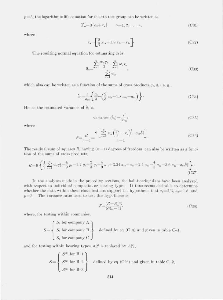
p = 3, the logarithmic life equation for the ath test group can be written as

a= I,2, ... , n, (0 31)

where

(032)

The r esulting normal equation for estimating ao is

n W Y n ~ --"-"-"- ~ WaXa

A a=1 3 a=1 ao= n ' (033)

~Wa a=1

which also can be written as a function of the sums of cross products gi , a ii> e. g. ,

A 1 { gO (2 )} ao= - '----- - a OI + 1.8 a02-a03 . aoo 3 3 (0:34)

H en ce the es tima ted variance of ao is

(0 35)

where

2 R s =--n - 1

9 [~ W", (~ -XaY-aooa&] n- l

(0 36)

The residual sum of squares R , having (n - l) degrees of freedom, can also b e written as a func­tion of th e sums of cross products,

In th e an alyses m ade in the preceding sec tions, the ball-bearing dat a h ave been an alyzed with respect to individual companies or bearing types. It thus seems desirable to determine whether the data within these classifications suppor t the hypothesis th at al = 2/3, a2 = 1.8, and p = 3. The variance r atio used to test this hypothesis is

where. for test ing within companies,

F= (R - S )/3, S/(n - 4)

( SI for companv A 'I

S = { 8 2 for compan~ B ~ defined by eq (013) and given in table 0 -1,

83 for company 0 J and for testing within b earing types, ai jl is r eplaced by Al'J,

{

S (I ) for B- 1 }

S = S (2) for B- 2

8 (3) for B-3

defined by eq (026) and given in table 0 - 2,

314

(0 ;)8)

and R (eq (C37» refers to the calculated residual sum of squares within the particular classil'ieation.

Table C- 3 summarizes with respect to companies A, B , and C the values of 0,0, R, the calculated F-l'atio (eq C38), and the critical F value. Table C--4 summarizes the same quan­tities for the B- 1, B- 2, and B- 3-type bearings made by company B .

The results of this analysis show that the values a l = 2/3, a2= 1.8, and p = 3 arc consistent for rating life LIO data with respect to each of the three compfmies. However, [01' median lifc L 50 , these assumed p ar ameter values are consistent only for the data from company A.

The resul ts for the same analysis made on the three different bearing types, indicate that the assumed parameter values are consistent only for the B- 1 and B- 2-type bearings with respect to median life L 50 •

It is interesting to note that the analysis for comp any B (ignoring bearing types) showed that the assumed values for the parameters arc consistent with the L lo data. However, a finer analysis by bearing type revealed that these values are not valid for the B- 3-type bear­ings. This app arent inconsistency sterns from the fact that t he analysis for company B , taken as a whole, is dominated by those bearing types h aving the larger number of test groups, i . e., B- 1 and B- 2, and for these types the parameter values were found to be consistent with the L IO data.

The estimates for i e, assuming a l = 2/3, (L2 = 1.8, and p = 3, arc summarized in table 8 of the main text for rating life L lO . This summary also includ es the value of i e for compall)' D eomputed from only three test grollps. (Because of the small number of tes t groups, it was not possible to verify whether the assumed pa,l'ameter values are vali d for these data.)

T A HI ,] , C- 3. S ummary of cOlltlmtations (by companies) to test hypothesis that data aTe consistent with assumed vallles al =2/3, a2= 1.8, 71 = 3

L iO L 50 Compan~' Criti cal

F ao= ln Ie I? F 60 = ln .re N F

A ___________________ 8. 4205 102. 539286 *- 0.06 8. 9382 94. 367916 O. 79 2. 80 B _______ ____________ 8. 5021 287. 613198 O. 42 8. 9254 217. 560672 3.7 1 2.65 C ___________________ 8. 1001 8. 375562 O. 96 8. 5832 8, 488584 9. 92 3. 59

*Kcgativc value due to rounding in calculations.

TABLE C- 4. Summary of computations (by beQ1'ing type) for company B to test hypothesis that data are consistent with assumed values al = 2/3, a2= 1.8, p= 3

LIO L 50 Type Critical

F 60 = ln .re R F ao = ln fe R F

B- 1 ____________ __ ___ 8. 4575 73. 821978 O. 84 8. 8636 44. 883126 3.95 2.86 B- 2 ___ ____ __ _______ _ 8. 5236 181. 128312 1. 17 8. 9482 141. 731604 2. 42 2. 70 B- 3 ______ ________ ___ 8. 5203 27.014247 5.81 9. 0022 18.905517 5. 21 3. 24

315

7 . References

[1] R. L. Anderson and T. A. Bancroft, Statistical theory in r esearch, ch. 13, 14, 15 (McGraw-Hill Book Co., Inc., New York, N. Y., 1952).

[2] H . Cramer, Mathematical methods of statistics (Princeton University Press, Princeton, N. J. , 1946). [3] VY. J. Dixon and F. J. Massey, Int roduction to statistical a nalysis, ch. 11 (McGraw-Hill Book Co., Inc.,

New York, N. Y., 1951). [4] M . A. Fieller, Some problems in interval estimation , J . Roy. Stat. Soc. [B] XVI, 175 (1954). [5] R. A. Fisher and L . H. C. Tippett, Limiting forms of the frequency distribut ion of t he largest or smallest

member of a sample, Proc. Cambridge Phil. Soc. 24, pt. 2, 180 (1928). [6] A. M. Freudenthal and E. J . Gumbel, On the statistical interpretation of fatigue tests, Proc. Royal Soc.

[A] 216, 309 (1953). [7] E. J. Gumbel, Les valeurs extremes des distributions statistiques, Ann. inst. H enri Poincare 5, p t. 2, 110

(1935) . [8] E. J . Gumbel, The return period of flood flows, Ann. Mat h. Stat. 12, 163 (June 1941). [9] E. J . Gumbel, Statistical theory of extreme values and some practical applications, National Bureau of

Standards Applied Mat hematics Series 33 (1954) (U. S. Government Print ing Offi ce, Washington 25, D . C.).

[10] A. I-laid, Statistical theory with engineering applications, ch. 18, 20 (John Wiley & Sons, New York, N. Y. , 1952).

[11] O. K empt horne, The design and analysis of experiments, ch. 4,5 (J ohn Wiley & Sons, New York, N. Y., 1952) .

[12] J . Lieblein , On the exact evaluation of the variances a nd covariances of order statistics in samples from the extreme-value distribut ion, Ann. Math. Stat. 24, 282 (June 1953).

[13] J. Lieblein, A new met hod of analyzin g extreme-value data, Nat. Advisory Comm. Aeronau. Tech. Note 3053 (J anuary 1954).

[14] J. Lieblein and H. E. Salzer, Table of t he first moment of ranked extremes (to be submitted to a technical journal) .

[15] G. Lundberg and A. P almgren, D ynamic capacity of rolling bearings, Acta Poly tech. 7, Mech. Eng. Series, 1 , No.3 (1947).

[16] A. M. Mood, Introduct ion to the theory of statistics, ch. 13 (McGraw-Hill Book Co., I nc., New York. N. Y ., 1950).

[17] Probability tables for the analysis of extreme-value data, National Bureau of Standards Applied Mathe­matics Series 22 (1953) (U. S. Government Printing Office, Washington 25, D. C.).

[18] W. Weibull, The phenomenon of rupture in solids, Ing. Vetenskaps Akad., H andl. No. 153 (1939) . [19] W. Wei bull, A statistical representat ion of fatigue fa ilure in solids, Trans. Roy . Inst. T echno!. , Stockholm.

No. 27 (1949). [20] S. S. Wilks, Mathematical statistics, ch. VIII (Princeton University Press, Princeton, N. J ., 1946), [21] S. S. Wilks, Order statistics, Bul. Am. Math. Soc. 54. 6 (J anuary 1948).

WASHINGTON, March 22, 1956.

316 U. S. GOVERNMENT PRINTING OFFICE: 1956