statistical inference for time-varying arch processessuhasini/papers/tvarch-annalsversion.pdf ·...
TRANSCRIPT
The Annals of Statistics2006, Vol. 34, No. 3, 1075–1114DOI: 10.1214/009053606000000227© Institute of Mathematical Statistics, 2006
STATISTICAL INFERENCE FOR TIME-VARYINGARCH PROCESSES1
BY RAINER DAHLHAUS AND SUHASINI SUBBA RAO
Universität Heidelberg
In this paper the class of ARCH(∞) models is generalized to the nonsta-tionary class of ARCH(∞) models with time-varying coefficients. For fixedtime points, a stationary approximation is given leading to the notation “lo-cally stationary ARCH(∞) process.” The asymptotic properties of weightedquasi-likelihood estimators of time-varying ARCH(p) processes (p < ∞)are studied, including asymptotic normality. In particular, the extra bias dueto nonstationarity of the process is investigated. Moreover, a Taylor expan-sion of the nonstationary ARCH process in terms of stationary processes isgiven and it is proved that the time-varying ARCH process can be written asa time-varying Volterra series.
1. Introduction. To model volatility in time series, Engle [6] introduced theARCH model where the conditional variance is stochastic and dependent on pastobservations. The ARCH model and several of its related models have gainedwidespread recognition because they model quite well the volatility in financialmarkets over relatively short periods of time (cf. [3, 13]). However, underlying allthese models is the assumption of stationarity. Now given the changing pace ofthe world’s economy, modeling financial returns over long intervals using station-ary time series models may be inappropriate. It is quite plausible that structuralchanges in financial time series may occur, causing the time series over long in-tervals to deviate significantly from stationarity. It is therefore plausible that, byrelaxing the assumption of stationarity in an adequate way, we may obtain a bet-ter fit. In this direction, Drees and Starica [5] have proposed the simple nonlinearmodel Xt = µ+σ(t)Zt , where Zt are independent, identically distributed randomvariables and σ(·) is a smooth function, which they estimate using a nonparametricregression method. Essentially, though it is not mentioned, the authors are treat-ing σ(t) as if it were of the form σ(t) = σ (t/N), with N being the sample size.Through this rescaling device it is possible to obtain a framework for a meaning-ful asymptotic theory. Feng [7] has also studied time inhomogeneous stochasticvolatility, by introducing a multiplicative seasonal and trend component into theGARCH model.
Received March 2003; revised July 2005.1Supported in part by the Deutsche Forschungsgemeinschaft (DA 187/12-1).AMS 2000 subject classifications. Primary 62M10; secondary 62F10.Key words and phrases. Derivative process, locally stationary, quasi-likelihood estimates, time-
varying ARCH process.
1075

1076 R. DAHLHAUS AND S. SUBBA RAO
In this paper we generalize the class of ARCH(∞) models (cf. [9, 16]) to mod-els with time-varying parameters:
Xt = σ(t)Zt where σ(t)2 = a0(t) +∞∑
j=1
aj (t)X2t−j ,(1)
and Zt are independent, identically distributed random variables with EZt = 0,EZ2
t = 1. As in nonparametric regression and in other work on nonparametric sta-tistics, we use the rescaling device to develop an asymptotic theory around such aclass of models, that is, we rescale the parameters to the unit interval [see (2) be-low]. The resulting process is called the time-varying ARCH (tvARCH) process.The same rescaling device has been used, for example, in nonparametric time se-ries by Robinson [15] and by Dahlhaus [4] in his definition of local stationaritywhich was essentially restricted to time-varying linear processes. We shall showin Section 2 that the tvARCH process can be locally approximated by station-ary ARCH processes. Therefore, this new class of tvARCH processes can also becalled locally stationary. The stationary ARCH approximation will later be used totransfer results for stationary ARCH processes to the locally stationary situation.
In Section 3 we study parameter estimation for tvARCH(p) models by weightedquasi-maximum likelihood methods. The nonstationarity of the process causes theestimator to be biased. We will show that the bias can be explained in terms ofthe derivatives of the tvARCH process. Furthermore, we will prove asymptoticnormality of the estimator.
In Section 4 we also define a special derivative of the tvARCH process and givea Taylor expansion of the nonstationary tvARCH process in terms of stationaryprocesses. This derivative enables us to study more precisely the nonstationarybehavior of the process. Moreover, the derivative process turns out to be a solutionof a stochastic differential equation.
In Section 5 time-varying Volterra series are studied. They are used to prove theexistence of a tvARCH(∞) process and to derive the results of Section 4 on itsderivatives. It is worth noting that the results in Section 5 are of independent inter-est and the methods used here can be generalized to other nonstationary processes.
In the Appendix we prove convergence theorems for ergodic stationaryprocesses and some specific convergence and approximation results for the like-lihood process. We also derive mixing properties of several processes, includingderivatives of the likelihood process.
2. The time varying ARCH process. In this section we broaden the class ofARCH(∞) models, by introducing nonstationary ARCH(∞) models with time-dependent parameters. In order to obtain a framework for a meaningful asymptotictheory, we rescale the parameter functions as in nonparametric regression and for

STATISTICAL INFERENCE FOR TIME-VARYING ARCH PROCESSES 1077
(linear) locally stationary processes to the unit interval, that is, we assume
Xt,N = σt,NZt
(2)where σ 2
t,N = a0
(t
N
)+
∞∑j=1
aj
(t
N
)X2
t−j,N for t = 1, . . . ,N,
where Zt are independent, identically distributed random variables with EZt = 0,EZ2
t = 1. We call the sequence of stochastic processes {Xt,N : t = 1, . . . ,N}which satisfy (2) a time-varying ARCH (tvARCH) process. As shown below,the tvARCH-process can be locally approximated by stationary ARCH processes.Therefore, we also call tvARCH processes locally stationary.
We mention that the rescaling technique is mainly introduced for obtaining ameaningful asymptotic theory, and by this device we can obtain adequate approx-imations for the nonrescaled case. In particular, the rescaling does not effect theestimation procedure. Furthermore, classical ARCH models are included as a spe-cial case (if the parameters are constant in time).
We make the following assumptions.
ASSUMPTION 1. The sequence of stochastic processes {Xt,N : t = 1, . . . ,N}has a time-varying ARCH representation defined in (2) where the parameters sat-isfy the following properties: There exist constants 0 < ρ,Q,M < ∞, 0 < ν < 1and a positive sequence {�(j)} such that infu a0(u) > ρ and
supu
aj (u) ≤ Q
�(j),(3)
Q
∞∑j=1
1
�(j)≤ (1 − ν),(4)
|aj (u) − aj (v)| ≤ M|u − v|�(j)
,(5)
where {�(j)} satisfies
∑j≥1
j
�(j)< ∞.
An example of such a positive sequence {�(j)} is
�(j) ={
1, j = 1,j2 log1+κ j, j > 1,
with some κ > 0 or �(j) = ηj for some η > 1. Condition (4) implies that E(X2t,N )
is uniformly bounded over t and N .

1078 R. DAHLHAUS AND S. SUBBA RAO
PROPOSITION 1. Under Assumption 1, {X2t,N } defined in (2) has an almost
surely well-defined unique solution in the set of all causal solutions. The solutionhas the form of a time-varying Volterra series expansion.
The proof for Proposition 1, as well as all the other proofs of results in thissection can be found in Section 5. We mention that a similar result also holds fornonrescaled tvARCH(∞) processes.
It is worth noting that throughout this paper we shall be working with X2t,N
rather than Xt,N , unless stated otherwise. This is because Xt,N can be randomly ei-ther positive or negative, whereas X2
t,N is always positive, allowing it to be unique.The smoothness of the parameters {aj (·)} guarantees that the process has (as-
ymptotically) locally a stationary behavior. We now make this notion precise. Thefirst point of interest is to study the stationary process which locally approximatesthe tvARCH-process in some neighborhood of a fixed point t0 (or in rescaledtime u0). For each given u0 ∈ (0,1], the stochastic process {Xt (u0)} is the sta-tionary ARCH process associated with the tvARCH(∞) process at time point u0if it satisfies
Xt (u0) = σt (u0)Zt ,(6)
where σt (u0)2 = a0(u0) +
∞∑j=1
aj (u0)Xt−j (u0)2
for all t ∈ Z. It is worth noting, if the parameters {aj (u0)} satisfy Assumption 1,then {Xt (u0)} is a stationary, ergodic ARCH(∞) process (cf. [9]).
Comparing (6) with (2), it seems clear that if t/N is close to u0, then X2t,N and
Xt (u0)2 should be close and the degree of the approximation should depend both
on the rescaling factor N and the deviation |t/N − u0|. This is shown below.
THEOREM 1. Suppose {Xt,N } is a tvARCH process which satisfies Assump-tion 1 and let Xt (u0) be defined as in (6). Then there exist a stationary, ergodic,positive process {Ut } independent of u0 with finite mean and a constant K inde-pendent of t and N such that
|X2t,N − Xt (u0)
2| ≤ K
(∣∣∣∣ t
N− u0
∣∣∣∣ + 1
N
)Ut a.s.(7)
We mention that an explicit formula for Ut is given in (48). As a consequenceof (7), we have
X2t,N = Xt (u0)
2 + Op
(∣∣∣∣ t
N− u0
∣∣∣∣ + 1
N
).
The bound in (7) allows us to approximate the local average of X2t,N by an average
of Xt (u0)2 (this is of particular interest here, since the local average and weighted
STATISTICAL INFERENCE FOR TIME-VARYING ARCH PROCESSES 1079
local average will be used frequently in later sections). For example, suppose |u0 −t0/N | < 1/N and we average X2
t,N about a neighborhood whose length (2M + 1)
increases as N increases but where the ratio M/N → 0 as N → ∞. Then byusing (7), we have
1
2M + 1
M∑k=−M
X2t0+k,N = 1
2M + 1
M∑k=−M
Xt0+k(u0)2 + RN,(8)
where RN is bounded by
|RN | ≤ KM
N
{1
2M + 1
M∑k=−M
Ut0+k
}P→ 0.
Thus, about the time point t0 the local average of a tvARCH process is asymp-totically the same as the local average of the stationary ARCH process {Xt (u0)
2}.Therefore, by using (7), we can locally approximate the tvARCH process by astationary process. The above approximation can be refined by using derivativeprocesses as defined in Section 4. By using them, we can find, for example, anexpression for the asymptotic bias RN in (8).
3. The segment quasi-likelihood estimate. In this section we consider a ker-nel type estimator of the parameters of a tvARCH(p) model given the sample{Xt,N : t = 1, . . . ,N}. The process {Xt,N } is assumed to satisfy the representation
Xt,N = σt,NZt ,
(9)where σ 2
t,N = a0
(t
N
)+
p∑j=1
aj
(t
N
)X2
t−j,N for t = 1 . . . ,N,
where Zt are independent, identically distributed random variables with EZt = 0,EZ2
t = 1. The order p is assumed known. We study the distributional propertiesof the estimator, including asymptotic normality. Furthermore, we will investigatethe bias of the estimator due to nonstationarity of the tvARCH(p) process. We willuse the following assumptions.
ASSUMPTION 2. The sequence of stochastic processes {Xt,N : t = 1, . . . ,N}has a tvARCH(p) representation defined by (9). Furthermore:
(i) The process satisfies Assumption 1.(ii) For some δ > 0,
E(|Zt |4(1+δ)) < ∞.(10)
(iii) Let � be the compact set
� ={α = (α0, α1, . . . , αp) :
p∑j=1
αj ≤ 1, ρ1 ≤ α0 ≤ ρ2, ρ1 ≤ αi for i = 1, . . . , p
},
1080 R. DAHLHAUS AND S. SUBBA RAO
where 0 < ρ1 ≤ ρ2 < ∞. For each u ∈ (0,1], we assume au ∈ Int(�), where au =(a0(u), a1(u), . . . , ap(u)).
(iv) The third derivative of aj (·) exists with
supu
∣∣∣∣∂iaj (u)
∂ui
∣∣∣∣ ≤ C
for i = 1,2,3 and j = 0,1, . . . , p, where C is a finite constant independent of i
and j .(v) The random variable Zt has a positive density on an interval containing
zero.(vi) [This assumption is only used in Theorem 3(ii)]
{E(Z120 )}1/6
p∑j=1
Q
�(j)≤ (1 − ν).
REMARK 1. (i) The conditions placed on the parameter space in Assump-tion 2(iii) can be relaxed to include all vectors α = (α0, α1, . . . , αp), where αi = 0for any i = 1, . . . , p, in the parameter space. By including these points, a methodfor model selection could be derived. However, the cost for relaxing this assump-tion is that additional moment conditions have to be placed on Xt,N .
(ii) We use Assumption 2(ii) to prove asymptotic normality of the estimator.Typically for stationary ARCH processes, the result can be proved if E(Z4
t ) < ∞.However, we require the mildly stronger assumption E(|Z|4+δ
t ) < ∞ to prove asimilar result for sums of martingale arrays as opposed to sums of martingale dif-ferences used in the stationary situation (cf. [10], Theorem 3.2). Assumption 2(vi)means that both E(X12
t,N ) and E(Xt (u)12) are uniformly bounded in t,N and u.We refer also to the comments on the moment assumptions in Section 6.
(iii) In Section 5 we apply a theorem of Basrak, Davis and Mikosch [1], whogave conditions under which a GARCH(p, q) process is mixing. Assumption 2(iii)is sufficient for the Lyapunov exponent of the random recurrence matrix associ-ated with {Xt (u)} to be negative. In addition, Assumption 2(iii), (v) is sufficientto ensure that the ARCH process {Xt (u)} is α-mixing of rate −∞ (see [1] andreferences therein).
We now define the segment (kernel) estimator of a(u0) for each u0 ∈ (0,1). Lett0 ∈ N such that |u0 − t0/N | < 1/N . The estimator considered in this section is theminimizer of the weighted conditional likelihood
Lt0,N (α) :=N∑
k=p+1
1
bNW
(t0 − k
bN
)�k,N(α),(11)
STATISTICAL INFERENCE FOR TIME-VARYING ARCH PROCESSES 1081
where
�k,N(α) = 1
2
(logwk,N(α) + X2
k,N
wk,N(α)
)(12)
with wk,N(α) = α0 +p∑
j=1
αjX2k−j,N
and W : [−1/2,1/2] → R is a kernel function of bounded variation with∫ 1/2−1/2 W(x)dx = 1 and
∫ 1/2−1/2 xW(x)dx = 0. That is, we consider
at0,N = arg minα∈�
Lt0,N (α).(13)
Obviously �t,N(α) is the conditional likelihood of Xt,N given Xt−1,N , . . . ,Xt−p,N
and the parameters α = (α0, . . . , αp)T , provided the Zt are normally distributed.All results below also hold if the Zt are not normally distributed but simply satisfyAssumption 2. For this reason (and the fact that the conditional likelihood is not thefull likelihood), the likelihood is called a quasi-likelihood. For later reference, welist the derivatives of �k,N(α). Let ∇ = ( ∂
∂α0, . . . , ∂
∂αp)T . Since ∇2wk,N(α) = 0,
we have
�k,N(α) = 1
2
{log(wk,N(α)) + X2
k,N
wk,N(α)
},(14)
∇�k,N(α) = 1
2
{∇wk,N(α)
wk,N(α)− X2
k,N∇wk,N(α)
wk,N(α)2
},(15)
∇2�k,N(α) = 1
2
{−∇wk,N(α)∇wk,N(α)T
wk,N(α)2(16)
+ 2X2
k,N∇wk,N(α)∇wk,N(α)T
wk,N(α)3
}.
at0,N is regarded as an estimator of at0/N = (a0(t0/N), . . . , ap(t0/N))T or of au0 ,where |u0 − t0/N | < 1/N .
In the derivation of the asymptotic properties of this estimator we make useof the local approximation of X2
t,N by the stationary process Xt (u0)2 defined in
Section 2. Similarly to the above, we therefore define the weighted likelihood
LN(u0,α) :=N∑
k=p+1
1
bNW
(t0 − k
bN
)�k(u0,α),(17)
where |u0 − t0/N | < 1/N and
�t (u0,α) = 1
2
(log wt (u0,α) + Xt (u0)
2
wt (u0,α)
)(18)
with wt (u0,α) = α0 +p∑
j=1
αj Xt−j (u0)2.

1082 R. DAHLHAUS AND S. SUBBA RAO
It is obvious that the same formulas as in (14)–(16) also hold for �k(u0,α) withX2
k,N and wk,N(α) replaced by Xk(u0)2 and wk(u0,α), respectively.
It is shown below that both Lt0,N (α) and LN(u0,α) converge to
L(u0,α) := E(�0(u0,α)
)(19)
as N → ∞, b → 0, bN → ∞ and |u0 − t0/N | < 1/N . It is easy to show thatL(u0,α) is minimized by α = au0 .
Furthermore, let
Bt0,N (α) := Lt0,N (α) − LN(u0,α)
=N∑
k=p+1
1
bNW
(t0 − k
bN
)(�k,N(α) − �k(u0,α)
).
(20)
Since LN(u0,α) is the likelihood of the stationary approximation, Xt (u0)Bt0,N (α)
is a bias caused by the deviation from stationarity. Lemma A.6 implies thatBt0,N (α) = Op(b). A better rate will be derived by a Taylor expansion in Propo-sition 3. Let
�(u0) = 1
2E
{∇w0(u0,au0)∇w0(u0,au0)T
w0(u0,au0)2
}.(21)
Since Xk(u0)/wk(u0,a0) = Z2k and Z2
k is independent of wk(u0,a0), we have
E(∇2�0
(u0,au0
)) = −�(u0)
and
E(∇ �0
(u0,au0
)∇ �0(u0,au0
)T ) = var(Z20)
2�(u0).
If Zt is Gaussian, then var(Z20) = 2.
LEMMA 1. Suppose {Xt,N : t = 1, . . . ,N} is a tvARCH(p) process which sat-isfies Assumption 2(i), (iii) and let LN(u0,α), L(u0,α) and Bt0,N be as definedby (17), (19) and (20), respectively. Then
supα∈�
|LN(u0,α) − L(u0,α)| P→ 0,(22)
supα∈�
∣∣Bt0,N (α)∣∣ P→ 0,(23)
supα∈�
|∇2LN(u0,α) − ∇2L(u0,α)| P→ 0(24)
and
supα∈�
∣∣∇2Bt0,N (α)∣∣ P→ 0,(25)
where b → 0 and bN → ∞ as N → ∞.
STATISTICAL INFERENCE FOR TIME-VARYING ARCH PROCESSES 1083
A direct implication of the lemma above is the following corollary.
COROLLARY 1. Let Lt,N (α) be as defined as in (11). Then under the assump-tions in Lemma 1, we have
supα∈�
∣∣Lt0,N (α) − L(u0,α)∣∣ P→ 0(26)
and
supα∈�
∣∣∇2Lt0,N (α) − ∇2L(u0,α)∣∣ P→ 0,(27)
where b → 0, bN → ∞ as N → ∞.
In the theorem below we show that at0,N is a consistent estimator of au0 .
THEOREM 2. Suppose {Xt,N : t = 1, . . . ,N} is a tvARCH(p) process whichsatisfies Assumption 2(i), (iii) and the estimator at0,N is as defined in (13). Then if|u0 − t0/N | < 1/N , we have
at0,NP→ a(u0),
where b → 0 and bN → ∞ as N → ∞.
PROOF. By using (26), we have pointwise convergence Lt0,N (a)P→ L(u0,a).
Since au0 = arg minα L(u0,α), we have
Lt0,N
(at0,N
) ≤ Lt0,N
(au0
) P→ L(u0,au0
) ≤ L(u0, at0,N
).
With (26), we now obtain Lt0,N (at0,N )P→ L(u0,au0). From the continuity of
L(u0, ·) and the compactness of the parameter space, we can now conclude
at0,NP→ au0 , provided L(u0, ·) has a unique solution. Since L(u0, ·) is the same
function as in the stationary case, this follows from Lemma 5.5 of [2]. �
We now prove asymptotic normality of the estimator with the usual Taylor ex-pansion argument. We have
∇Lt0,N
(at0,N
)i − ∇Lt0,N
(au0
)i = {∇2Lt0,N
(ait0,N
)(at0,N − au0
)}i ,(28)
with ait0,N
between at0,N and au0 . Since au0 is in the interior of �, we have√bN∇Lt0,N (at0,N )i
P→ 0. Since ait0,N
P→ au0 and supα∈� |∇2Lt0,N (α) −∇2L(u0,α)| P→ 0 [see (27)], then ∇2Lt0,N (ai
t0,N)
P→ −�(u0). Note that �(u0)
is nonsingular. This follows from Lemma 5.7 of [2] since �(u0) is the same as inthe stationary case.

1084 R. DAHLHAUS AND S. SUBBA RAO
Therefore, the distributional properties of at0,N − au0 are determined by∇Lt0,N (au0). By using (20), we see that
∇Lt0,N
(au0
) = ∇LN
(u0,au0
) + ∇Bt0,N
(au0
),(29)
which is essentially a decomposition into a stochastic and a bias part [although∇Bt0,N (au0) is also random, but its variance is of a lower order—see the detailsbelow]. The bias measures the deviation from stationarity and will disappear fora suitable choice of bandwidth b (see Proposition 2 and Theorem 3 below). Bysubstituting (29) into (28), we have
√bN
((at0,N − au0
) + �(u0)−1∇Bt0,N
(au0
))= √
bN�(u0)−1∇LN
(u0,au0
) + op(1).
Thus, the asymptotic distribution of (at0,N − au0) is determined by ∇LN(u0,au0).Note that this is the gradient of the likelihood of the stationary process Xt (u0)
2
however, with kernel weights. Since
∇ �k
(u0,au0
) = 1
2
(1 − Z2k )∇wk(u0,au0)
wk(u0,au0)(30)
is a martingale difference, ∇LN(u0,au0) is the weighted sum of martingale dif-ferences.
PROPOSITION 2. Suppose {Xt,N : t = 1, . . . ,N} is a tvARCH(p) processwhich satisfies Assumption 2(i), (ii), (iii) and LN(u0,au0) is as defined in (17).Then if |u0 − t0/N | < 1/N we have
√bN∇LN
(u0,au0
) D→ N
(0,w2
var(Z20)
2�(u0)
),(31)
where b → 0, bN → ∞, N → ∞ and w2 = ∫ 1/2−1/2 W(x)2 dx.
PROOF. Since ∇LN(u0,au0) is the weighted sum of martingale differences,the result follows from the martingale central limit and the Cramér–Wold device. Itis straightforward to check the conditional Lindeberg condition and the conditionalvariance condition. We omit the details. �
We now consider the stochastic bias ∇Bt0,N (au0). By using (30) andLemma A.6, we immediately get the relation
∇Bt0,N
(au0
) = Op(b).(32)
This bound together with the Proposition 2 leads to the assertion of Theorem 3(i)below. As mentioned above, the stochastic bias is a measure for the deviation of
STATISTICAL INFERENCE FOR TIME-VARYING ARCH PROCESSES 1085
the process {�t,N (au0)} from stationarity. This deviation depends on the rate ofchange of the parameters {aj (u)}. Under stronger moment conditions, we will nowdetermine this bias. To achieve this, we replace ∇�k,N(au0) by ∇ �k(
kN
,au0):
∇Bt0,N
(au0
) = ∑k
1
bNW
(t0 − k
bN
)(∇ �k
(k
N,au0
)− ∇ �k
(u0,au0
)) + RN,(33)
where
RN = ∑k
1
bNW
(t0 − k
bN
)(∇�k,N
(au0
) − ∇ �k
(k
N,au0
)).
Corollary A.1 now implies∣∣∣∣∇�k,N
(au0
) − ∇ �k
(k
N,au0
)∣∣∣∣ ≤ K
N
(Uk + (1 + Z2
k )
p∑j=1
Uk−j
),
with some constant K uniformly in k. Lemma 1 together with the independenceof Z2
k and Uk−j now imply
E(R2N)1/2 = O
(1
N
).
Suppose for each j = 0, . . . , p the third derivative of aj (·) exists and is uniformlybounded. Then by using Corollary 3 and taking a Taylor expansion of ∇ �k(u,au0)
about u = u0, we have
∇ �k
(k
N,au0
)− ∇ �k
(u0,au0
) =(
k
N− u0
)∂∇ �k(u,au0)
∂u
⌋u=u0
+ (k/N − u0)2
2
∂2∇ �k(u,au0)
∂u2
⌋u=u0
+ (k/N − u0)3
3!∂3∇ �k(u,au0)
∂u3
⌋u=Uk
,
(34)
where the random variable Uk ∈ (0,1]. A detailed investigation of the differentterms now leads to the following result on ∇Bt0,N (au0). We mention that, in par-ticular, the expectation of the first term cancels out.
PROPOSITION 3. Suppose {Xt,N : t = 1, . . . ,N} is a tvARCH(p) processwhich satisfies Assumption 2 and W is a kernel function of bounded variationwith
∫ 1/2−1/2 W(x)dx = 1 and
∫ 1/2−1/2 W(x)x dx = 0. Then if |u0 − t0/N | < 1/N , we
have
E(∇Bt0,N
(au0
)) = 1
2b2w(2)
∂2∇L(u,au0)
∂u2
⌋u=u0
+ O
(b3 + 1
N
)

1086 R. DAHLHAUS AND S. SUBBA RAO
and
var(∇Bt0,N
(au0
)) = O
(b6 + 1
N
),
where w(2) = ∫ 1/2−1/2 W(x)x2 dx.
A detailed proof can be found in Appendix A.4.Propositions 2 and 3 and (32) give us the distributional properties of the estima-
tor at0,N , which we summarize in the theorem below.
THEOREM 3. Suppose {Xt,N : t = 1, . . . ,N} is a tvARCH(p) process whichsatisfies Assumption 2(i), (ii), (iii) and W is a kernel function of bounded variationwith
∫ 1/2−1/2 W(x)dx = 1 and
∫ 1/2−1/2 W(x)x dx = 0. Then if |u0 − t0/N | < 1/N , we
have the following:
(i) If b3 � N−1, then√
bNBt0,N (au0)P→ 0 and
√bN
(at0,N − au0
) D→ N
(0,w2
var(Z20)
2�(u0)
−1).
(ii) If in addition Assumption 2(iv), (v), (vi) holds and b13 � N−1, then√
bN�(u0)−1∇Bt0,N
(au0
) = √bNb2µ(u0) + op(1)
and
√bN
(at0,N − au0
) + √bNb2µ(u0)
D→ N
(0,w2
var(Z20)
2�(u0)
−1),(35)
where
µ(u0) = 1
2w(2)�(u0)
−1 ∂2∇L(u,au0)
∂u2
⌋u=u0
.(36)
REMARK 2. (i) We recall the structure of this result: The asymptotic Gaussiandistribution is the same as for the stationary approximation. In addition, we havea bias term which comes from the deviation of the true process from the station-ary approximation on the segment. In particular, this bias term is zero if the trueprocess is stationary. A simple example is given below. By estimating and mini-mizing the mean squared error (i.e., by balancing the variance and the bias due tononstationarity on the segment), we may find an estimator for the optimal segmentlength.
(ii) If EZ40 = 3, as in the case of normally distributed Zt , then
√bN
(at0,N − au0
) + √bNb2µ(u0)
D→ N(0,w2�(u0)
−1).
STATISTICAL INFERENCE FOR TIME-VARYING ARCH PROCESSES 1087
(iii) It is clear from Propositions 2 and 3 that
E∥∥�(u0)
−1Bt0,N
(au0
)∥∥22 = b4‖µ(u0)‖2
2 + O
(b6 + 1
N
)
and
E∥∥�(u0)
−1∇LN
(u0,au0
)∥∥22 = w2
var(Z20)
2bNtrace(�(u0)
−1) + o
(1
bN
).
Therefore, if b13 � N−1, using the above, we conjecture that
E∥∥at0,N − au0
∥∥22
= b4‖µ(u0)‖22 + w2
var(Z20)
2bNtrace(�(u0)
−1) + o
(b4 + 1
bN
).
(37)
However, this is very hard to prove. The b which minimizes the conjectured meansquare error would be the theoretical optimal bandwidth (i.e., the optimal segmentlength).
(iv) We illustrate the above results with an example. We first consider thetvARCH(0) process
Xt,N = σt,NZt , σ 2t,N = a0
(t
N
),
which Drees and Starica [5] have also studied. In this case ∂Xt (u)2
∂u= a′
0(u)Z2t and
under Assumption 2, we have
∂2∇L(u,au0)
∂u2
⌋u=u0
= −1
2
a′′0 (u0)
a0(u0)2 and �(u0) = 1
2a0(u0)2 ,
that is,
µ(u0) = −12w(2)a′′
0 (u0).
This example illustrates well how the bias is linked to the nonstationarity of theprocess—if the process were stationary, the derivatives of a0(·) would be zero,causing the bias also to be zero. Conversely, sudden variations in a0(·) about thetime point u0 would be reflected in a′′
0 (u0) and manifest as a large µ(u0). Straight-forward minimization of the first two summands in (37) leads to the optimal band-width, which in this case (and for Gaussian Zt ) takes the form
bopt =(
2w2
w(2)2
)1/5
N−1/5[a0(u0)
a′′0 (u0)
]2/5
,
leading to a large bandwidth if a′′0 (u0) is small and vice versa. Thus, the optimal
choice of the bandwidth (of the segment length) depends on the degree of sta-tionarity of the process. For general tvARCH(p) processes µ(u0) is very hard toevaluate. Furthermore, it assumes a very complicated form.
1088 R. DAHLHAUS AND S. SUBBA RAO
(v) It is of interest to investigate whether the differences in the kernel-QMLat each time point are because the true ARCH parameters are time-varying or aresimply due to random variation in the estimation method. From a practical point ofview, one could evaluate the sum of squared deviations between the kernel-QMLestimator at each time point and the global QML estimator. We conjecture that theasymptotic distribution under the null hypothesis of stationarity is a chi-square.
4. The derivative process. A key element to the proof of Theorem 3 is thenotion of the derivative of the process Xt (u)2 with respect to u and the result-ing Taylor expansion for the nonstationary process X2
t,N in terms of stationaryprocesses as given in Corollary 2 below. Since these “derivative processes” areof general interest, we introduce them in this section for general tvARCH(∞)
processes Xt,N as given in (2) and Xt (u) given in (6). We need the followingstronger regularity conditions on the parameters.
ASSUMPTION 3. The third derivative of {aj (·)} exists. Furthermore,
supu
∣∣∣∣∂iaj (u)
∂ui
∣∣∣∣ ≤ C
�(j)for i = 1,2,3 and j = 0,1, . . . ,(38)
where �(j) is defined as in Assumption 1 and C is a finite constant independent ofi and j .
THEOREM 4. Suppose Assumptions 1 and 3 hold and let {Xt (u)} be defined as
in (6). Then the derivatives { ∂Xt (u)2
∂u}, { ∂2Xt (u)2
∂u2 } and { ∂3Xt (u)2
∂u3 } are almost surelywell defined unique stationary stochastic processes for each u ∈ (0,1). Further-
more, ∂Xt (u)2
∂uis almost surely the unique solution of the stochastic differential
equation
∂Xt (u)2
∂u=
(a′
0(u) +∞∑
j=1
a′j (u)Xt−j (u)2 +
∞∑j=1
aj (u)∂Xt−j (u)2
∂u
)Z2
t ,(39)
where a′j (u) denotes the derivative of aj (u) with respect to u.
Note that (39) is just the derivative of (6) with σt (u)2 replaced by Xt (u)2/Z2t .
An explicit formula for ∂Xt (u)2
∂uis given in (51). Similar expressions also hold for
the second and third derivatives. For example, if all the derivatives of aj (·) werezero also the derivative process would be zero [in this case X2
t,N would be station-
ary and Xt (u)2 = X2t,N for all u].
An important consequence of Theorem 4 is that it allows us to make a Taylorexpansion of Xt (u)2 about u0 (rigourously proved in Section 5), to give
Xt (u)2 = Xt (u0)2 + (u − u0)
∂Xt (u)2
∂u
⌋u=u0
+ 1
2(u − u0)
2 ∂2Xt (u)2
∂u2
⌋u=u0
+ Op
((u − u0)
3).
(40)

STATISTICAL INFERENCE FOR TIME-VARYING ARCH PROCESSES 1089
An interesting feature of the Taylor expansion in (40) is that it does not dependon the existence of moments of Xt (u)2, unlike other types of series expansions.Instead the expansion depends on the smoothness of the parameters aj (·).
The approximation in (7), where X2t,N = Xt (
tN
)2 + Op(1/N), and the Taylorexpansion in (40) lead to the corollary below.
COROLLARY 2. Suppose {Xt,N } is a tvARCH process which satisfies Assump-tions 1 and 3 and let Xt (u) be defined as in (6). Then for any u0 ∈ (0,1], we have
X2t,N = Xt (u0)
2 +(
t
N− u0
)∂Xt (u)2
∂u
⌋u=u0
+ 1
2
(t
N− u0
)2 ∂2Xt (u)2
∂u2
⌋u=u0
+ Op
((t
N− u0
)3
+ 1
N
).
(41)
The nice feature of the result of Corollary 2 is that it gives a Taylor expansion ofthe nonstationary process X2
t,N around Xt (u0)2 in terms of stationary processes.
This is particularly nice since it allows use of well-known results for stationaryprocesses (such as the ergodic theorem) in describing properties of Xt,N . A sim-ilar result also holds for higher-order expansions with higher-order derivatives.However, in this paper only a second-order expansion is needed.
As an example, we now use (41) to derive a tighter bound for the remain-der RN in (8). The effect is similar as in nonparametric regression: Due to theanti-symmetry of the kernel weights, the expectation of the first term falls out. Byusing (41), we have, for |t0/N − u0| < 1/N ,
RN = 1
2M + 1
M∑k=−M
k
N
∂Xt0+k(u)2
∂u
⌋u=u0
+ 1
2M + 1
M∑k=−M
1
2
(k
N
)2 ∂2Xt0+k(u)2
∂u2
⌋u=u0
+ Op
((M
N
)3
+ 1
N
)
= T1 + T2 + Op
((M
N
)3
+ 1
N
).
The expectation of T1 is zero. Under the additional condition E(Z40)1/2 ∑
j Q/
�(j) ≤ (1 − ν), { ∂Xt (u)2
∂u} is a short memory process in which case var(T1) =
O(M/N2) (see Lemmas A.7 and A.10). Thus, T2 dominates T1 in probability andwe have
RN = 1
2M + 1
M∑k=−M
1
2
(k
N
)2 ∂2Xt0+k(u)2
∂u2
⌋u=u0
+ Op
((M
N
)3
+(√
M
N
)).
Note that this is a (stochastic) bias of the approximation in (8).

1090 R. DAHLHAUS AND S. SUBBA RAO
Theorem 4 and Corollary 2 can easily be generalized to include derivatives offunctions of tvARCH processes. By using the chain and product rules, we havethe generalization below, which we use to study the quasi-likelihood defined inSection 3.
COROLLARY 3. Suppose Assumptions 1 and 3 hold, let {Xt (u)} be as definedin (6) and f : Rd → R, where the first, second and third derivatives of f exist.
(i) Then
∂f (Xt1(u)2, . . . , Xtd (u)2)
∂u=
d∑i=1
∂Xti (u)2
∂u
∂f
∂Xti (u)2,
∂2f (Xt1(u)2, . . . , Xtd (u)2)
∂u2 =d∑
i=1
∂2Xti (u)2
∂u2
∂f
∂Xti (u0)2
+d∑
i,j=1
∂Xti (u)2
∂u
∂Xtj (u)2
∂u
× ∂2f
∂Xti (u0)2 ∂Xtj (u0)2.
(42)
Furthermore, by using the product and chain rules, similar expressions can be
obtained for ∂3f
∂u3 .
(ii) Suppose f : Rd → R is differentiable with uniformly bounded third deriva-tive. Then we have
f(X2
t+t1,N, . . . ,X2
t+td ,N
) = f (Xt (u)2) +(
t
N− u0
)∂f (Xt (u)2)
∂u
⌋u=u0
+ (t/N − u0)2
2
∂2f (Xt (u)2)
∂u2
⌋u=u0
+ Op
((t
N− u0
)3
+ 1
N
),
(43)
where Xt (u)2 := (Xt+t1(u)2, . . . , Xt+td (u)2)T .
5. Volterra expansions of tvARCH processes. In this section we prove theexistence and uniqueness of the process Xt,N and of the derivative process fromSection 4. This is done by means of Volterra expansions. The methods used herecan easily be generalized to include other nonstationary stochastic processes whichhave as their solution a Volterra expansion. Therefore, the results and methods inthis section are of independent interest. A treatise of ordinary Volterra expansionscan be found in [14].

STATISTICAL INFERENCE FOR TIME-VARYING ARCH PROCESSES 1091
Giraitis, Kokoszka and Leipus [9] have shown that a unique solution of Xt (u)2,defined in (6), is almost surely the Volterra series given by
Xt (u)2 = a0(u)Z2t + ∑
k≥1
mt (u, k),(44)
where
mt (u, k) = ∑j1,...,jk≥1
a0(u)
(k∏
r=1
ajr (u)
)k∏
r=0
Z2t−∑r
s=1 js
= ∑jk<···<j0:j0=t
gu(k, j0, j1, . . . , jk)
k∏i=0
Z2ji,
with
gu(k, j0, j1, . . . , jk) = a0(u)
k∏i=1
a(ji−1−ji )(u).
We now show a similar result is true for X2t,N . Let aj (u) = 0 for u < 0 and
j ≥ 0. A formal expansion of X2t,N , defined in (2), gives
X2t,N = a0
(t
N
)Z2
t + ∑k≥1
mt,N(k),(45)
where
mt,N(k) = ∑j1,...,jk≥1
a0
(t − ∑k
s=1 js
N
)(k∏
r=1
ajr
(t − ∑r−1
s=1 js
N
))(k∏
r=0
Z2t−∑r
s=1 js
)
= ∑jk<···<j0 : j0=t
gt,N (k, j0, j1, . . . , jk)
k∏i=0
Z2ji,
with
gt,N(k, j0, j1, . . . , jk) = a0
(jk
N
) k∏i=1
a(ji−1−ji )
(ji−1
N
).
We stated in Proposition 1 that the tvARCH process has a unique solution. We nowprove this result by showing that (45) is the unique solution. The proof in manyrespects is close to the proof of Theorem 2.1 in [9].
PROOF OF PROPOSITION 1. We first show that (45) is well defined. Since (45)is the sum of positive random variables and the coefficients are also positive, we

1092 R. DAHLHAUS AND S. SUBBA RAO
only need to show that the expectation of (45) is finite. By using (3), (4) and themonotone convergence theorem, a bound for the expectation of (45) is
E(X2t,N ) ≤ sup
ua0(u) + sup
ua0(u)
∞∑k=1
∑jk<···<j0 : j0=t
k∏i=1
Q
�(ji − ji−1)
≤ supu
a0(u)
[1 +
∞∑k=1
(1 − ν)k
]< ∞.
(46)
Furthermore, it is not difficult to see that X2t,N is a well-defined solution of (2).
To show uniqueness of X2t,N , we must show that any other solution is equal
to X2t,N with probability one. Suppose Y 2
t,N is a solution of (2). By recursivelyapplying relation (2) r times to Y 2
t,N , we have
Y 2t,N = a0
(t
N
)+
r−1∑k=1
mt,N(k)+ ∑jr<···<j0 : j0=t
gt,N(r, j0, . . . , jr)Y 2
jr ,N
a0(jr/N)
r−1∏i=0
Z2ji.
Thus, the difference between Y 2t,N and X2
t,N is
X2t,N − Y 2
t,N = Ar − Br,
where
Ar =∞∑
k=r
mt,N(k)
and
Br = ∑jr<···<j0 : j0=t
gt,N (r, j0, . . . , jr)Y 2
jr ,N
a0(jr/N)
r−1∏i=0
Z2ji.
We now show, for any ε > 0, that∑∞
r=1 P(|Ar − Br | > ε) < ∞. By us-ing (3) and (4), we have E(Ar) ≤ C(1 − ν)r . Furthermore, since Y 2
t,N is
causal, Y 2jr ,N
and∏r−1
i=0 Z2ji
are independent (if i < r , then ji > jr ). Therefore,
E(Y 2jr ,N
∏r−1i=0 Z2
ji) = E(Y 2
jr ,N) and we have
E(Br) = ∑jr<···<j0 : j0=t
gt,N(r, j0, . . . , jr)E(Y 2
jr ,N)
a0(jr/N)
≤ 1
infu a0(u)supt,N
E(Y 2t,N )(1 − ν)r .
Now by using the Markov inequality, we have P(Ar > ε) ≤ C1(1 − ν)r/ε andP(Br > ε) ≤ C1(1 − ν)r/ε for some constant C1. Therefore, P(|Ar − Br | > ε) ≤
STATISTICAL INFERENCE FOR TIME-VARYING ARCH PROCESSES 1093
C2(1 − ν)r/ε. Thus,∑∞
r=1 P(|Ar − Br | > ε) < ∞ and by the Borel–Cantellilemma, the event {|Ar − Br | > ε} can occur only finitely often with probabilityone. Since this is true for all ε > 0, we have Yt,N
a.s.= Xt,N and therefore the re-quired result. �
REMARK 3. It is worth noting that mt,N(k) can be obtained by using the re-cursion
mt,N(k) = Z2t
∑j≥1
aj
(t
N
)mt−j,N (k − 1) for k ≥ 2,
with the initial condition
mt,N(1) = Z2t
∑j≥1
aj
(t
N
)Z2
t−j .
Our object now is to prove Theorem 1, that is, to bound the difference betweenX2
t,N and Xt (u0)2. More precisely, we will prove under Assumption 1 that
|X2t,N − Xt (u0)
2| ≤ K
(∣∣∣∣ t
N− u0
∣∣∣∣ + 1
N
)Ut,(47)
where
Ut = Z2t +
∞∑k=1
Qk−1∑
jk<···<j0 : j0=t
k|j0 − jk|∏ki=1 �(ji−1 − ji)
k∏i=0
Z2ji
(48)
is a stationary ergodic positive process with finite expectation.
PROOF OF THEOREM 1. To prove (47), we use the triangle inequality to get
|X2t,N − Xt (u0)
2| ≤∣∣∣∣X2
t,N − Xt
(t
N
)2∣∣∣∣ +∣∣∣∣Xt
(t
N
)2
− Xt (u0)2∣∣∣∣
and consider bounding |X2t,N − Xt (
tN
)2| and |Xt (tN
)2 − Xt (u0)2| separately. By
using (44) and (45), we have∣∣∣∣X2
t,N − Xt
(t
N
)2∣∣∣∣≤ ∑
k≥1
∑jk<···<j0 : j0=t
|gt,N(k, j0, j1, . . . , jk)
− gt/N(k, j0, j1, . . . , jk)|k∏
i=0
Z2ji.
(49)
1094 R. DAHLHAUS AND S. SUBBA RAO
We notice j0/N = t/N . By successively replacing a(ji−1−ji )(ji−1N
) by
a(ji−1−ji )(j0N
), by using (3), the Lipschitz continuity of the parameters in (5) andthat (j0 − jk) ≥ (j0 − ji) (for i ≤ k) and (j0 − jk) = ∑k
i=1(ji−1 − ji), we have
|gt,N(k, j0, j1, . . . , jk) − gt/N(k, j0, j1, . . . , jk)|≤ KQk−1 k|j0 − jk|
N∏k
i=1 �(ji − ji−1),
(50)
where K is a finite constant. Therefore, by using (49) and (50), we have∣∣∣∣X2t,N − Xt
(t
N
)2∣∣∣∣ ≤ K1
NUt .
Now we bound |Xt (tN
) − Xt (u0)2|. By using (44), we have∣∣∣∣Xt (u0)
2 − Xt
(t
N
)2∣∣∣∣≤
∣∣∣∣a0(u0) − a0
(t
N
)∣∣∣∣Z2t
+ ∑k≥1
∑jk<···<j0 : j0=t
∣∣gu0(k, j0, j1, . . . , jk) − gt/N (k, j0, j1, . . . , jk)∣∣ k∏i=0
Z2ji.
By using similar methods to those given above, we have∣∣∣∣Xt (u0)2 − Xt
(t
N
)2∣∣∣∣ ≤ K
∣∣∣∣ t
N− u0
∣∣∣∣Ut .
Therefore, we have shown (47).We now show that Ut is a well-defined stochastic process. Since Ut is the sum
of positive random variables, we only need to show that E(Ut ) < ∞. Taking theexpectation of Ut , using (4) and the independence of {Z2
t }, we have
E(Ut ) = 1 +∞∑
k=1
∑jk<···<j0 : j0=t
kQk−1 |j0 − jk|∏ki=1 �(ji − ji−1)
≤ 1 + L
∞∑k=1
k2(1 − ν)k−1 < ∞,
where L = ∑∞j=1 j/�(j) [L is finite by definition of �(j)]. Thus, {Ut } is a well-
defined process with finite mean. By using Stout [17], Theorem 3.5.8, we can showthat {Ut } is an ergodic process. Hence, we have the result. �
We now prove Theorem 4 on the existence of the derivatives of Xt (u)2 withrespect to u. We will show that this is given by sums of the derivatives of the

STATISTICAL INFERENCE FOR TIME-VARYING ARCH PROCESSES 1095
mt (u, k) terms in (44), that is,
∂Xt (u)2
∂u= a′
0(u)Z2t + a′
0(u)∑k≥1
∑j1,...,jk≥1
(k∏
r=1
ajr (u)
)k∏
r=0
Z2t−∑r
s=1 js
+ a0(u)∑k≥1
k∑n=1
∑j1,...,jk≥1
a′jn
(u)
(k∏
r=1,r �=n
ajr (u)
)k∏
r=0
Z2t−∑r
s=1 js.
(51)
This leads to the Taylor expansions of Xt (u)2 [as stated in (40)] and finally to theTaylor-type representation of X2
t,N stated in Corollary 2. The latter two results are
proved below. Throughout the rest of the section X2t,N (ω), Xt (u,ω)2, and so on,
denote a specific realization of X2t,N , Xt (u)2.
PROOF OF THEOREM 4. From (44), we know that Xt (u)2 has almost surelya Volterra series expansion, given by (44), as its unique solution. Therefore, thereexists a subset N1(u) of the event space where P(N1(u)c) = 1 and
Xt (u,ω)2 = a0(u)Zt(ω)2
+ a0(u)∑k≥1
∑j1,...,jk≥1
(k∏
r=1
ajr (u)
)k∏
r=0
Zt−∑rs=1 js
(ω)2(52)
∀ω ∈ N1(u)c. Furthermore, since the random process {Ut }, defined in (48), is welldefined (see Theorem 1), there exists a set N2 with P(N c
2 ) = 1 and Ut(ω) finite,for all ω ∈ N c
2 . For ω ∈ N3(u)c = N1(u)c ∩ N c2 , we consider realizations of the
right-hand side of (51) and
Vt = supu
|a′0(u)|Z2
t + supu
|a′0(u)| ∑
k≥1
∑j1,...,jk≥1
(k∏
r=1
supu
ajr (u)
)k∏
r=0
Z2t−∑r
s=1 js
+ supu
a0(u)∑k≥1
k∑n=1
∑j1,...,jk≥1
supu
∣∣a′jn
(u)∣∣( k∏
r=1,r �=n
supu
ajr (u)
)k∏
r=0
Z2t−∑r
s=1 js.
We will now use the following result: Suppose f (x) = ∑∞j=1 gj (x) for x ∈ [0,1],
where f is a deterministic function. It is well known if∑∞
j=1 g′j (x) is uniformly
convergent [which is true if∑∞
j=1 supx |g′j (x)| < ∞], the derivatives are finite
and∑∞
j=1 gj (x) converges at least at one point, then f ′(x) = ∑∞j=1 g′
j (x). We
now use this result to show that the derivative of Xt (u)2 is well defined. Supposeω ∈ N3(u)c. Then by using (52) and (48), we have
Xt (u,ω)2 ≤ max(1,Q) supu
a0(u)Ut(ω) < ∞,
1096 R. DAHLHAUS AND S. SUBBA RAO
where the summands in Ut(ω) are absolutely and uniformly summable. Further-more, under Assumption 3 and (4), we have, for all ω ∈ N3(u)c,
Vt(ω) ≤(
supu
|a′0(u)| + C
Qsupu
|a0(u)|)Ut(ω) < ∞.
Therefore, ∂Xt (u,ω)2
∂u= Yt (u,ω) is almost surely given by (51). By using [17], The-
orem 3.5.8, it is clear { ∂Xt (u)2
∂u} is an ergodic process.
To show that (51) is the unique solution of (39), we can use the same method asgiven in the proof of Theorem 1. We omit the details here.
We can use the same method as described above to show that { ∂2Xt (u)2
∂u2 } and
{ ∂3Xt (u)2
∂u3 } are uniquely well-defined ergodic processes. Again, we omit the details.�
At this point it is easy to derive some moment conditions on Xt (u) and itsderivatives.
LEMMA 2. Suppose {Xt,N : t = 1, . . . ,N} is a tvARCH(∞) process whichsatisfies Assumptions 1 and 3 and, in addition,
E(Z2r0 )1/r
∑j
Q
�(j)< (1 − ν)
for r ≥ 1. Then E|Ut |r < ∞, E| supu Xt (u)2|r < ∞, E| supu∂Xt (u)2
∂u|r < ∞ and
E| supu∂2Xt (u)2
∂u2 |r < ∞ uniformly in t .
PROOF. The result follows by applying the Minkowski inequality to (48),(44), (51) and the corresponding formula for the second derivative and using argu-ments similar to those in (46). We omit the details. �
PROOF OF (40) AND COROLLARY 2. We first prove (40). For ω ∈ N3(u)c ∩N3(u0)
c, with N3 as defined above, the Volterra series expansions (44) give so-lutions of (6) for Xt (u)2 and Xt (u0)
2. The relation (40) now follows from an or-
dinary Taylor expansion of Xt (u,ω)2 about u0, noting that E( ∂3Xt (u)3
∂u3 �u=U
) < ∞for an arbitrary random variable U .
By using (40) and∣∣∣∣X2
t,N − Xt
(t
N
)2∣∣∣∣ ≤ K
NUt,
we obtain Corollary 2. �
STATISTICAL INFERENCE FOR TIME-VARYING ARCH PROCESSES 1097
6. Concluding remarks. We have studied the class of nonstationaryARCH(∞) processes with time-varying coefficients. We have shown that, abouta given time point, the process can be approximated by a stationary process.Moreover, this approximation has facilitated the Taylor expansion of the tvARCHprocess in terms of stationary processes. It is worth mentioning that the existenceof the derivatives of the coefficients determines the existence of the derivativesof the process and the subsequent Taylor expansion (and not the existence of themoments). The definition of the derivative process and the Taylor expansion is notrestricted to tvARCH(∞) processes, and with simple modifications can also beapplied to other nonstationary processes.
To estimate the time-varying parameters of a time-varying ARCH(p) (p < ∞)process, we have used a weighted quasi-likelihood on a segment. Investigation ofthe asymptotic properties of the estimator showed an extra bias due to nonstation-arity on the segment. This expression can be used to find an adaptive choice ofthe segment length (by minimizing, e.g., the mean squared error and estimatingthe second derivative). The relevance of this model for (say) financial data needsfurther investigation. We conjecture that, by using tvARCH models, the often dis-cussed long range dependence of the squared log returns can be reduced drasticallyand even disappear completely (there has been some discussion that the long rangedependence of the squares is in truth only due to some nonstationarity in the data;see [12]). Furthermore, we conjecture that, for example, the empirical kurtosis offinancial log returns is much smaller with a time-varying model than with a clas-sical ARCH model.
Typically for stationary ARCH(p) processes, the existence of E(Z40) is assumed
in order to show asymptotic normality of the quasi-likelihood estimator. A draw-back of our approach is that the expression of the bias given in (36) holds onlyunder the assumption [E(Z12
0 )]1/6 ∑pj=1
Q�(j)
≤ (1− ν), that is, under the existence
of the 12th moment. However, if we assume the weaker condition E(Z4+δ0 ) < ∞,
then the segment quasi-likelihood estimator still has asymptotically a normal dis-tribution, but the explicit form of the bias cannot be evaluated (see also Remark 1).
We mention that, unlike the case of stationary GARCH(p, q) models, thetime-varying GARCH model is not included in the tvARCH(∞) class. Theinvestigation of time-varying GARCH(p, q) models is a topic of future research.However, unlike tvGARCH models, the squares of certain tvARCH(∞) modelshave “near” long memory behavior (cf. [9, 11]). This is one justification for study-ing tvARCH(∞)-models.
An important issue not discussed in this paper are the practical aspects whenthe model is applied. In particular, identifiability requires investigation since bothconditional heteroscedasticity and time varying parameters are suitable to modelvolatility. Theoretically the model is identifiable and we are convinced this alsoholds in practice for large data sets. However, it has to be checked whether this
1098 R. DAHLHAUS AND S. SUBBA RAO
leads to satisfactory results for moderate sample sizes. Our idea is that the condi-tional heteroscedasticity models the short term fluctuations, while the time varyingparameters model the longer term changes. Of course this can be achieved by asufficiently large choice of the bandwidth.
APPENDIX
In this appendix we establish the results required in the proofs of Section 3.Many of the results related to the local quasi-likelihood defined at (11) depend
on the asymptotic limit of the weighted sum of nonstationary random processes.The general method we use to deal with such sums is to substitute an ergodicprocess for the nonstationary process, and to study the limit of a weighted sum ofan ergodic process. In Appendix A.1 we establish results related to the weightedsums of ergodic processes. These results are used in Appendix A.2, where we studythe difference between the nonstationary tvARCH process and the correspondingapproximating stationary processes. We then use this result to evaluate the limitof weighted sums of functions of tvARCH(p) processes. In Appendix A.3 weinvestigate the mixing properties of the likelihood process and in Appendix A.4the bias of the segment estimate from Section 3.
A.1. Convergence results for weighted sums of random variables. In thissection we prove ergodic type theorems for weighted sums of ergodic processes.In the lemma below we show an almost sure convergence result and in Lemma A.2we prove convergence in probability for certain triangular arrays.
LEMMA A.1. Suppose {Yt } is an ergodic sequence with E|Yt | < ∞ andW : [−1/2,1/2] → R is a kernel function of bounded variation with∫ 1/2−1/2 W(x)dx = 1. Then
M∑k=−M
1
2M + 1W
(k
2M + 1
)Yk
a.s.→ µ as M → ∞,
where µ = E(Y0).
PROOF. SinceM∑
k=−M
1
2M + 1W
(k
2M + 1
)→
∫ 1/2
−1/2W(x)dx = 1,(A.1)
we can assume without loss of generality that µ = 0. We split the sum into negativeand positive suffixed elements, which gives
SM = 1
2M + 1
0∑k=−M
W
(k
2M + 1
)Yk + 1
2M + 1
M∑k=1
W
(k + M
2M + 1
)Yk
= NM + PM,
(A.2)
STATISTICAL INFERENCE FOR TIME-VARYING ARCH PROCESSES 1099
and consider first PM . By using summation by parts, we have, with Sk = ∑ki=1 Yi ,
PM = 1
2M + 1
M−1∑k=1
[W
(k
2M + 1
)− W
(k + 1
2M + 1
)]Sk
+ 1
2M + 1W
(M
2M + 1
)SM.
Since W is of bounded variation, this yields
|PM | ≤ K
2M + 1supk≤M
|Sk|
with some constant K . Now the ergodic theorem implies Sk(ω)/k → 0 for almostall ω. It is obvious for these ω that also PM(ω) tends to zero. In the same way weconclude that NM → 0 a.s., which gives the result. �
For kernel estimates about arbitrary center points, the situation is more difficultsince we basically average over triangular arrays of observations. We thereforeprove in the following lemma only convergence in probability.
LEMMA A.2. Suppose {Yt } is an ergodic sequence with E|Yt | < ∞ andW : [−1/2,1/2] → R is a kernel function of bounded variation with∫ 1/2−1/2 W(x)dx = 1. Then
µN(u0) :=N∑
k=p+1
1
bNW
(u0 − k/N
b
)Yk
P→ µ for u0 ∈ [0,1],(A.3)
where b → 0, bN → ∞ as N → ∞, and µ = E(Y0).
PROOF. Again we consider only the case µ = 0. Suppose N ≥ N0 withN0 such that u0 − p/N0 > b0/2 and u0 − 1 < −b0/2, b0 = b(N0) [i.e., thesum in (A.3) is over the whole domain of W ]. Let k0 = k0(N) be such that|u0 − k0/N | < 1/N . Since {Yk} is stationary, µN(u0) has the same distributionas ∑
k
1
bNW
(u0 − k/N
b
)Yk−k0 = ∑
k
1
bNW
(u0 − k0/N − k/N
b
)Yk
= µN
(u0 − k0
N
).
Since W is of bounded variation, this is equal to
∑k
1
bNW
(− k
bN
)Yk + RN

1100 R. DAHLHAUS AND S. SUBBA RAO
with RN ≤ KbN
sup−bN<k<bN |Yk|. Lemma A.1 implies that the first term convergesto zero almost surely [the proof of Lemma A.1 remains the same with (2M + 1)
replaced by bN ]. Since |Yk| ≤ |Sk|+ |Sk−1|, where Sk = ∑ki=1 Yi , the second term
also converges to zero almost surely (as in the proof of Lemma A.1). Therefore,
P(|µN(u0)| ≥ ε
) = P(|µN(u0 − k0/N)| ≥ ε
) → 0,
which gives the result. �
A.2. Convergence of the local likelihood and its derivatives. In this sectionwe evaluate the limit of weighted sums of {�t,N(α)}, {∇�t,N(α)}, {∇2�t,N(α)} andthe corresponding stationary approximations. In particular, we prove Lemma 1.Recall the formulas (14)–(16) and the corresponding formulas for �t (u0,α). Letκ = ρ2+1
ρ1and
�t,N := �t,N(u0,Ut ,α)
:=p∑
j=1
αj
{∣∣∣∣ t − j
N− u0
∣∣∣∣ + 1
N
}Ut−j ,
(A.4)
with the ergodic process Ut from (48). For a better understanding of the followingresult, we note that we have, for |u0 − t0
N| < 1/N , E(�t0,N (u0,Ut ,α)) = O(N−1)
and therefore,
�t0,N (u0,Ut ,α) = Op(N−1),
uniformly in u0 and α. The same holds for Z2t0�t0,N since Z2
t and �t,N are inde-pendent with E(Z2
t ) = 1.In the following lemmas we derive upper bounds for the expressions occurring
in (14), (15) and (16) and for the difference between these expressions and thecorresponding expressions in �t (u0,α) and its derivatives. Assumption 2(iii) im-mediately yields
∇wt,N(α)i
wt,N (α)≤ 1
ρ1,
∇wt (u0,α)i
wt (u0,α)≤ 1
ρ1(A.5)
uniformly in t , N , u0 and α (i = 1, . . . , p + 1).
LEMMA A.3. Suppose {Xt,N : t = 1, . . . ,N} is a tvARCH(p) process whichsatisfies Assumption 2(i), (iii). Then
X2t,N
wt,N(α)≤ κZ2
t andXt (u)2
wt (u,α)≤ κZ2
t .(A.6)
STATISTICAL INFERENCE FOR TIME-VARYING ARCH PROCESSES 1101
PROOF. We only prove (A.6) for the tvARCH case; the proof for the stationarycase is similar. Since X2
t,N = Z2t,Nσ 2
t,N , we have
X2t,N
wt,N(α)= Z2
t
(σ 2
t,N
wt,N(α)
)
= Z2t
(a0(t/N) + ∑pj=1 aj (t/N)X2
t−j,N
α0 + ∑pj=1 αjX
2t−j,N
)
≤ Z2t
(a0(t/N)
α0+
p∑j=1
aj (t/N)
αj
)
≤ κZ2t .
The last line is true because∑p
j=1 aj (t/N) < 1 and αj > ρ1 for j = 0, . . . , p. �
LEMMA A.4. Under the assumptions of Lemma A.3, we have
X2t,N
wt,N(α)= Xt (u0)
2
wt (u0,α)+ R1,N (u0, t),
(A.7)where |R1,N (u0, t)| ≤ 1
ρ1
(∣∣∣∣ t
N− u0
∣∣∣∣)Ut + κ
ρ1Z2
t �t,N (u0,Ut ,α),
∇wt,N(α)i
wt,N (α)= ∇wt (u0,α)i
wt (u0,α)+ R2,N (u0, t) (i = 1, . . . , p + 1),
(A.8)where |R2,N (u0, t)| ≤ 2
ρ21
�t,N(u0,Ut ,α)
and
log(wt,N(α)) = log(wt (u0,α)) + R3,N (u0, t),(A.9)
where |R3,N (u0, t)| ≤ 1
ρ1�t,N(u0,Ut ,α).
PROOF. We first prove (A.7). We have
|R1,N (u0, t)| ≤∣∣∣∣ X2
t,N
wt,N(α)− Xt (u0)
2
wt,N(α)
∣∣∣∣ +∣∣∣∣ Xt (u0)
2
wt,N(α)− Xt (u0)
2
wt (u0,α)
∣∣∣∣≤ 1
ρ1|X2
t,N − Xt (u0)2|
+ Xt (u0)2
ρ1wt (u0,α)|wt,N(α) − wt (u0,α)|.
(A.10)
1102 R. DAHLHAUS AND S. SUBBA RAO
From the definitions of wt,N(α) and wt (u0,α) and by using (7), we have
|wt,N(α) − wt (u0,α)| ≤p∑
j=1
αj
{∣∣∣∣ t − j
N− u0
∣∣∣∣ + 1
N
}Ut−j
≤ �t,N(u0,Ut ,α).
(A.11)
Together with (7) and (A.6), this leads to (A.7). Since ∇wt,N(α)i = X2t+1−i,N for
i = 2, . . . , p + 1, the proof of (A.8) is almost the same, so we omit the details. Thecase i = 1 also follows in the same way.
We now prove (A.9). By differentiating log(wt,N(α)) with respect to X2t−j,N
and using the mean value theorem, we have
R3,N (u0, t) = 1
α0 + ∑pj=1 αjYj
p∑j=1
αj
(X2
t−j,N − Xt−j (u0)2)
,(A.12)
where (Yj : i = 1, . . . , p) are positive random variables [since both X2t−i,N and
Xt−i(u0)2 are positive and Yj lies in between]. Therefore, by using (7), we have
|R3,N (u0, t)| ≤ 1
ρ1
( p∑j=1
αj
{∣∣∣∣ t − j
N− u0
∣∣∣∣ + 1
N
}Ut−j
)≤ 1
ρ1�t,N(u0,Ut ,α),
which is the required result. �
COROLLARY A.1. Under the assumptions of Lemma A.3, we have, for n ∈ N,∏nr=1 ∇wt,N(α)ir
wt,N (α)n=
∏nr=1 ∇wt (u0,α)ir
wt (u0,α)n+ R4,N (u0, t),
(A.13)where |R4,N (u0, t)| ≤ 2n
ρn+11
�t,N(u0,Ut ,α)
and
X2t,N
∏n−1r=1 ∇wt,N(α)ir
wt,N (α)n= Xt (u0)
2 ∏n−1r=1 ∇wt (u0,α)ir
wt (u0,α)n+ R5,N (u0, t),
(A.14)where |R5,N (u0, t)| ≤ 1
ρn1
(∣∣∣∣ t
N− u0
∣∣∣∣ + 1
N
)Ut + 2κn
ρn1
Z2t �t,N (u0,Ut ,α),
where 0 < ir ≤ p for r = 1, . . . , n.
PROOF. We can prove (A.13) by successively replacing ∇wt,N(α)ir /wt,N(α)
by ∇wt (u0,α)ir /wt (u0,α) for r = 1, . . . , n. Then by using (A.8) and the boundαir > ρ1 for all α ∈ �, we have the result. We can prove (A.14) by using a similarmethod as above together with (A.6) and (A.7). We omit the details here. �

STATISTICAL INFERENCE FOR TIME-VARYING ARCH PROCESSES 1103
LEMMA A.5. Suppose {Xt,N } is a tvARCH(p) process which satisfies As-sumption 2(i), (iii) and W is a kernel function of bounded variation with∫ 1/2−1/2 W(x)dx = 1. Then we have
N∑k=p+1
1
bNW
(t0 − k
bN
)Xk(u0)
2 ∏n−1r=1 ∇wk(u0,α)ir
wk(u0,α)n
P→ E
(X0(u0)
2 ∏n−1r=1 ∇w0(u0,α)ir
w0(u0,α)n
),
(A.15)
N∑k=p+1
1
bNW
(t0 − k
bN
)∏nr=1 ∇wk(u0,α)ir
wk(u0,α)nP→ E
(∏nr=1 ∇w0(u0,α)ir
w0(u0,α)n
)(A.16)
andN∑
k=p+1
1
bNW
(t0 − k
bN
)log
(wk(u0,α)
) P→ E(log
(w0(u0,α)
)).(A.17)
PROOF. Since ∇wt (u0,α)irwt (u0,α)
≤ 1/ρ1, we have by using (A.6) that
Xt (u0)2 ∏n−1
r=1 ∇wt (u0,α)ir
wt (u0,α)n≤ κZ2
t
ρn1
.
By using [17], Theorem 3.5.8, the process { Xt (u0)2 ∏n−1
r=1 ∇wt (u0,α)irwt (u0,α)n
}t is ergodic andby using the bound above has finite mean. By applying Lemma A.2, we have ver-ified (A.15).
Since logρ1 ≤ log wt (u0,α) ≤ (logρ2 + (1/ρ1)∑p
j=1 αj Xt−j (u0)2),
log wt (u0,α) has a finite mean. (A.16) and (A.17) follow similarly. �
LEMMA A.6. Under the assumptions of Lemma A.5 and |t0/N − u0| < 1/N
with u0 ∈ (0,1), we have, for all n ∈ N,
supα∈�
N∑k=p+1
1
bNW
(t0 − k
bN
)∣∣∣∣X2k,N
∏n−1r=1 ∇wk,N(α)ir
wk,N(α)n
(A.18)
− Xk(u0)2 ∏n−1
r=1 ∇wk(u0,α)ir
wk(u0,α)n
∣∣∣∣ = Op(b),
supα∈�
N∑k=p+1
1
bNW
(t0 − k
bN
)∣∣∣∣∏n
r=1 ∇wk,N(α)ir
wk,N(α)n
(A.19)
−∏n
r=1 ∇wk(u0,α)ir
wk(u0,α)n
∣∣∣∣ = Op(b)

1104 R. DAHLHAUS AND S. SUBBA RAO
and
supα∈�
N∑k=p+1
1
bNW
(t0 − k
bN
)∣∣log(wk,N(α)
) − log(wk(u0,α)
)∣∣ = Op(b).(A.20)
PROOF. Let
RN = supα∈�
N∑k=p+1
1
bNW
(t0 − k
bN
)∣∣∣∣X2k,N
∏n−1r=1 ∇wk,N(α)ir
wk,N(α)n
− Xk(u0)2 ∏n−1
r=1 ∇wk(u0,α)ir
wk(u0,α)n
∣∣∣∣.We note first that if α ∈ �, then αi ≤ max(1, ρ2), where αi is the ith element ofthe (p + 1)-dimensional vector α. By using (A.14) and | k−j
N− u0| ≤ | k−j
N− p|
when k lies in the support of W(t0−kbN
), we have the bound
|RN | ≤ C
(b + p + 1
N
) N∑k=p+1
1
bNW
(t0 − k
bN
)Vk = C
(b + p + 1
N
)LN,
where Vk ={Uk + Z2
k
p∑j=1
Uk−j
}
and C is a finite constant. Since Ut−j (by Theorem 1) and Z2t have finite mean and
are independent when j ≥ 1, {Vt } has a finite mean. Therefore, by using (A.3), we
have that LNP→ E(V0) and |RN | = Op(b). Thus, we have proved (A.18).
By using (A.13) and (A.9), we can obtain (A.19) and (A.20) similarly. �
PROOF OF LEMMA 1. We first show (22). To prove uniform convergence, itis sufficient to show both pointwise convergence and equicontinuity in probabilityof LN(u0,α) (since � is compact). By using (A.15) and (A.17), for every α ∈ �,we have
LN(u0,α) = 1
2
N∑k=p+1
1
bNW
(t0 − k
bN
)
×(
log(wk(u0,α)
) + Xk(u0)2
wk(u0,α)
)
P→ L(u0,α),
where b → 0, bN → ∞ as N → ∞. We now show equicontinuity in probabil-ity of LN(u0,α). By the mean value theorem, for every α1,α2 ∈ �, there exists
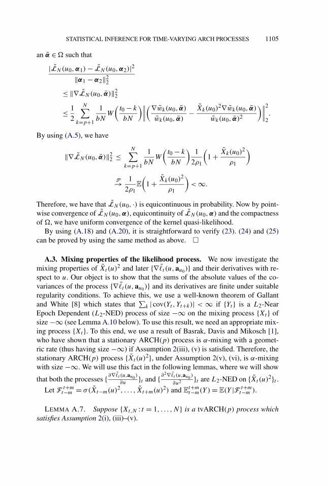
STATISTICAL INFERENCE FOR TIME-VARYING ARCH PROCESSES 1105
an α ∈ � such that
|LN(u0,α1) − LN(u0,α2)|2‖α1 − α2‖2
2
≤ ‖∇LN(u0, α)‖22
≤ 1
2
N∑k=p+1
1
bNW
(t0 − k
bN
)∥∥∥∥(∇wk(u0, α)
wk(u0, α)− Xk(u0)
2∇wk(u0, α)
wk(u0, α)2
)∥∥∥∥2
2.
By using (A.5), we have
‖∇LN(u0, α)‖22 ≤
N∑k=p+1
1
bNW
(t0 − k
bN
)1
2ρ1
(1 + Xk(u0)
2
ρ1
)
P→ 1
2ρ1E
(1 + Xk(u0)
2
ρ1
)< ∞.
Therefore, we have that LN(u0, ·) is equicontinuous in probability. Now by point-wise convergence of LN(u0,α), equicontinuity of LN(u0,α) and the compactnessof �, we have uniform convergence of the kernel quasi-likelihood.
By using (A.18) and (A.20), it is straightforward to verify (23). (24) and (25)can be proved by using the same method as above. �
A.3. Mixing properties of the likelihood process. We now investigate themixing properties of Xt (u)2 and later {∇ �t (u,au0)} and their derivatives with re-spect to u. Our object is to show that the sums of the absolute values of the co-variances of the process {∇ �t (u,au0)} and its derivatives are finite under suitableregularity conditions. To achieve this, we use a well-known theorem of Gallantand White [8] which states that
∑k | cov(Yt , Yt+k)| < ∞ if {Yt } is a L2-Near
Epoch Dependent (L2-NED) process of size −∞ on the mixing process {Xt } ofsize −∞ (see Lemma A.10 below). To use this result, we need an appropriate mix-ing process {Xt }. To this end, we use a result of Basrak, Davis and Mikosch [1],who have shown that a stationary ARCH(p) process is α-mixing with a geomet-ric rate (thus having size −∞) if Assumption 2(iii), (v) is satisfied. Therefore, thestationary ARCH(p) process {Xt (u)2}, under Assumption 2(v), (vi), is α-mixingwith size −∞. We will use this fact in the following lemmas, where we will show
that both the processes { ∂∇�t (u,au0 )
∂u}t and { ∂2∇�t (u,au0 )
∂u2 }t are L2-NED on {Xt (u)2}t .Let F t+m
t−m = σ(Xt−m(u)2, . . . , Xt+m(u)2) and Et+mt−m(Y ) = E(Y |F t+m
t−m ).
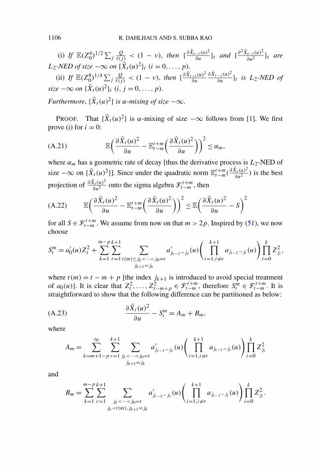
LEMMA A.7. Suppose {Xt,N : t = 1, . . . ,N} is a tvARCH(p) process whichsatisfies Assumption 2(i), (iii)–(v).
1106 R. DAHLHAUS AND S. SUBBA RAO
(i) If E(Z40)1/2 ∑
jQ
�(j)< (1 − ν), then { ∂Xt−i (u)2
∂u}t and { ∂2Xt−i (u)2
∂u2 }t are
L2-NED of size −∞ on {Xt (u)2}t (i = 0, . . . , p).
(ii) If E(Z80)1/4 ∑
jQ
�(j)< (1 − ν), then { ∂Xt−i (u)2
∂u
∂Xt−j (u)2
∂u}t is L2-NED of
size −∞ on {Xt (u)2}t (i, j = 0, . . . , p).
Furthermore, {Xt (u)2} is α-mixing of size −∞.
PROOF. That {Xt (u)2} is α-mixing of size −∞ follows from [1]. We firstprove (i) for i = 0:
E
(∂Xt (u)2
∂u− E
t+mt−m
(∂Xt (u)2
∂u
))2
≤ αm,(A.21)
where αm has a geometric rate of decay [thus the derivative process is L2-NED of
size −∞ on {Xt (u)2}]. Since under the quadratic norm Et+mt−m(∂Xt (u)2
∂u2 ) is the best
projection of ∂Xt (u)2
∂u2 onto the sigma algebra F t+mt−m , then
E
(∂Xt (u)2
∂u− E
t+mt−m
(∂Xt (u)2
∂u
))2
≤ E
(∂Xt (u)2
∂u− S
)2
(A.22)
for all S ∈ F t+mt−m . We assume from now on that m > 2p. Inspired by (51), we now
choose
Smt = a′
0(u)Z2t +
m−p∑k=1
k+1∑r=1
∑t (m)≤jk<···<j0=t
jk+1=jk
a′jr−1−jr
(u)
(k+1∏
i=1,i �=r
aji−1−ji(u)
)k∏
i=0
Z2ji,
where t (m) = t − m + p [the index jk+1 is introduced to avoid special treatmentof a0(u)]. It is clear that Z2
t , . . . ,Z2t−m+p ∈ F t+m
t−m , therefore Smt ∈ F t+m
t−m . It isstraightforward to show that the following difference can be partitioned as below:
∂Xt (u)2
∂u− Sm
t = Am + Bm,(A.23)
where
Am =∞∑
k=m+1−p
k+1∑r=1
∑jk<···<j0=t
jk+1=jk
a′jr−1−jr
(u)
(k+1∏
i=1,i �=r
aji−1−ji(u)
)k∏
i=0
Z2ji
and
Bm =m−p∑k=1
k+1∑r=1
∑jk<···<j0=t
jk<t(m),jk+1=jk
a′jr−1−jr
(u)
(k+1∏
i=1,i �=r
aji−1−ji(u)
)k∏
i=0
Z2ji.
STATISTICAL INFERENCE FOR TIME-VARYING ARCH PROCESSES 1107
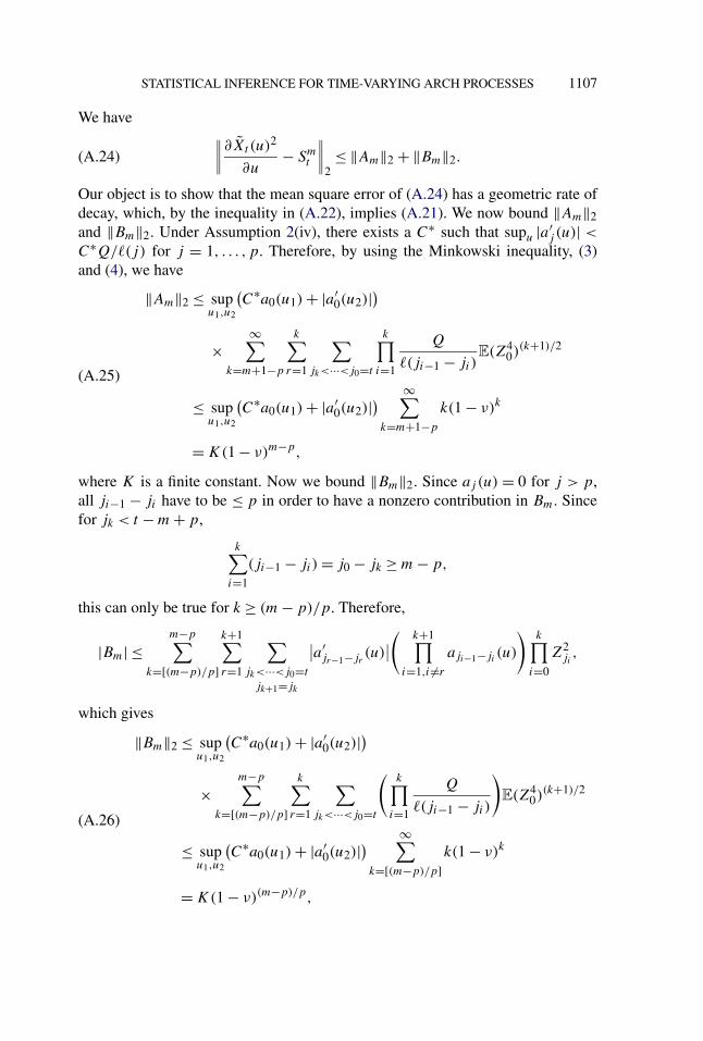
We have ∥∥∥∥∂Xt (u)2
∂u− Sm
t
∥∥∥∥2≤ ‖Am‖2 + ‖Bm‖2.(A.24)
Our object is to show that the mean square error of (A.24) has a geometric rate ofdecay, which, by the inequality in (A.22), implies (A.21). We now bound ‖Am‖2and ‖Bm‖2. Under Assumption 2(iv), there exists a C∗ such that supu |a′
j (u)| <
C∗Q/�(j) for j = 1, . . . , p. Therefore, by using the Minkowski inequality, (3)and (4), we have
‖Am‖2 ≤ supu1,u2
(C∗a0(u1) + |a′
0(u2)|)
×∞∑
k=m+1−p
k∑r=1
∑jk<···<j0=t
k∏i=1
Q
�(ji−1 − ji)E(Z4
0)(k+1)/2
≤ supu1,u2
(C∗a0(u1) + |a′
0(u2)|) ∞∑k=m+1−p
k(1 − ν)k
= K(1 − ν)m−p,
(A.25)
where K is a finite constant. Now we bound ‖Bm‖2. Since aj (u) = 0 for j > p,all ji−1 − ji have to be ≤ p in order to have a nonzero contribution in Bm. Sincefor jk < t − m + p,
k∑i=1
(ji−1 − ji) = j0 − jk ≥ m − p,
this can only be true for k ≥ (m − p)/p. Therefore,
|Bm| ≤m−p∑
k=[(m−p)/p]
k+1∑r=1
∑jk<···<j0=t
jk+1=jk
∣∣a′jr−1−jr
(u)∣∣( k+1∏
i=1,i �=r
aji−1−ji(u)
)k∏
i=0
Z2ji,
which gives
‖Bm‖2 ≤ supu1,u2
(C∗a0(u1) + |a′
0(u2)|)
×m−p∑
k=[(m−p)/p]
k∑r=1
∑jk<···<j0=t
(k∏
i=1
Q
�(ji−1 − ji)
)E(Z4
0)(k+1)/2
≤ supu1,u2
(C∗a0(u1) + |a′
0(u2)|) ∞∑k=[(m−p)/p]
k(1 − ν)k
= K(1 − ν)(m−p)/p,
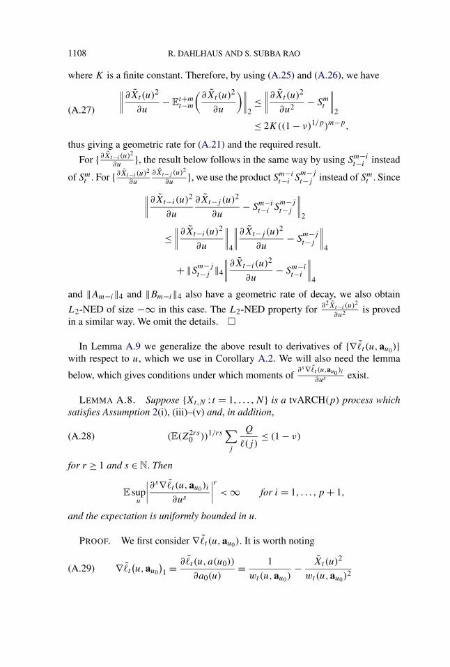
(A.26)
1108 R. DAHLHAUS AND S. SUBBA RAO
where K is a finite constant. Therefore, by using (A.25) and (A.26), we have∥∥∥∥∂Xt (u)2
∂u− E
t+mt−m
(∂Xt (u)2
∂u
)∥∥∥∥2≤
∥∥∥∥∂Xt (u)2
∂u2 − Smt
∥∥∥∥2
≤ 2K((1 − ν)1/p)m−p,
(A.27)
thus giving a geometric rate for (A.21) and the required result.
For { ∂Xt−i (u)2
∂u}, the result below follows in the same way by using Sm−i
t−i instead
of Smt . For { ∂Xt−i (u)2
∂u
∂Xt−j (u)2
∂u}, we use the product Sm−i
t−i Sm−jt−j instead of Sm
t . Since
∥∥∥∥∂Xt−i(u)2
∂u
∂Xt−j (u)2
∂u− Sm−i
t−i Sm−jt−j
∥∥∥∥2
≤∥∥∥∥∂Xt−i(u)2
∂u
∥∥∥∥4
∥∥∥∥∂Xt−j (u)2
∂u− S
m−jt−j
∥∥∥∥4
+ ‖Sm−jt−j ‖4
∥∥∥∥∂Xt−i(u)2
∂u− Sm−i
t−i
∥∥∥∥4
and ‖Am−i‖4 and ‖Bm−i‖4 also have a geometric rate of decay, we also obtain
L2-NED of size −∞ in this case. The L2-NED property for ∂2Xt−i (u)2
∂u2 is provedin a similar way. We omit the details. �
In Lemma A.9 we generalize the above result to derivatives of {∇ �t (u,au0)}with respect to u, which we use in Corollary A.2. We will also need the lemma
below, which gives conditions under which moments of∂s∇�t (u,au0 )i
∂us exist.
LEMMA A.8. Suppose {Xt,N : t = 1, . . . ,N} is a tvARCH(p) process whichsatisfies Assumption 2(i), (iii)–(v) and, in addition,
(E(Z2rs0 ))1/rs
∑j
Q
�(j)≤ (1 − ν)(A.28)
for r ≥ 1 and s ∈ N. Then
E supu
∣∣∣∣∂s∇ �t (u,au0)i
∂us
∣∣∣∣r
< ∞ for i = 1, . . . , p + 1,
and the expectation is uniformly bounded in u.
PROOF. We first consider ∇ �t (u,au0). It is worth noting
∇ �t
(u,au0
)1 = ∂�t (u, a(u0))
∂a0(u)= 1
wt(u,au0)− Xt (u)2
wt(u,au0)2(A.29)

STATISTICAL INFERENCE FOR TIME-VARYING ARCH PROCESSES 1109
and
∇ �t
(u,au0
)i = ∂�t (u, a(u0))
∂ai−1(u)
= Xt−i+1(u)2
wt(u,au0)− Xt (u)2Xt−i+1(u)2
wt(u,au0)2
(A.30)
for i = 2, . . . , p + 1. We first prove the result for the case s = 1. By using Corol-lary 3(i), we have
∂∇ �t (u,au0)i
∂u=
p∑j=0
∂Xt−j (u)2
∂u
∂∇ �t (u,au0)i
∂Xt−j (u)2.(A.31)
By using (A.29) and (A.30), if au0 ∈ �, we have
∣∣∣∣∂∇ �t (u,au0)i
∂Xt (u)2
∣∣∣∣ ≤ K and∣∣∣∣∂∇ �t (u,au0)i
∂Xt−j (u)2
∣∣∣∣ ≤ K(1 + Z2t )
(A.32)for j = 1, . . . , p,
where K is a finite constant. By using (A.31), (A.32) and the independence of Z2t
and ∂Xt−j (u)
∂u, we obtain
∣∣∣∣∂∇ �t (u,au0)i
∂u
∣∣∣∣ ≤∣∣∣∣∂Xt (u)2
∂u
∣∣∣∣ + K
p∑j=1
(1 + Z2t )
∣∣∣∣∂Xt−j (u)2
∂u
∣∣∣∣,thus, ∥∥∥∥∂∇ �t (u,au0)i
∂u
∥∥∥∥r
≤∥∥∥∥∂Xt (u)2
∂u
∥∥∥∥r
+ K
p∑j=1
∥∥∥∥(1 + Z2t )
∂Xt−j (u)2
∂u
∥∥∥∥r
(A.33)
≤∥∥∥∥∂Xt (u)2
∂u
∥∥∥∥r
+ K
p∑j=1
‖1 + Z2t ‖r
∥∥∥∥∂Xt−j (u)2
∂u
∥∥∥∥r
.
(A.28) and Lemma 2 now imply the result.To prove the similar result for the higher order derivatives (s > 1), we use the
same method as above. But in this case we require stronger conditions on the mo-ments of Xt (u)2 [see (A.28)]. The proof is straightforward and we omit the detailshere. �
We now use the result above to show that { ∂∇�t (u,au0 )i
∂u} is L2-NED on {Xt (u)2}.
LEMMA A.9. Suppose {Xt,N } is a tvARCH(p) process which satisfies As-sumption 2(i), (iii)–(v).

1110 R. DAHLHAUS AND S. SUBBA RAO
(i) If (E(Z40))1/2 ∑
jQ
�(j)≤ (1 − ν), then the process
{∂∇ �t (u,au0)i
∂u
}t
is L2-NED of size −∞ on {Xt (u)2}.(ii) If (E(Z8
0))1/4 ∑j
Q�(j)
≤ (1 − ν), then the process
{∂2∇ �t (u,au0)i
∂u2
}t
is L2-NED of size −∞ on {Xt (u)2}.
PROOF. We first prove (i). Let m > 2p. By using (A.32), we have
∥∥∥∥∂∇ �t (u,au0)i
∂u− E
t+mt−m
(∂∇ �t (u,au0)i
∂u
)∥∥∥∥2
≤p∑
j=0
∥∥∥∥∂∇ �t (u,au0)i
∂Xt−j (u)2
{∂Xt−j (u)2
∂u− E
t+mt−m
(∂Xt−j (u)2
∂u
)}∥∥∥∥2
≤ K
[∥∥∥∥∂Xt (u)2
∂u− E
t+mt−m
(∂Xt (u)2
∂u
)∥∥∥∥2
+ ‖(1 + Z2t )‖2
p∑j=1
∥∥∥∥{∂Xt−j (u)2
∂u− E
t+mt−m
(∂Xt−j (u)2
∂u
)}∥∥∥∥2
].
Lemma A.7 now implies that { ∂∇�t (u,au0 )i
∂u}t is L2-NED of size −∞ on {Xt (u)2}t .
The proof for the second derivative process is similar, but requires the strongermoment condition given in (ii). We omit the details of the proof. �
We now state a theorem of Gallant and White [8] which we use in Corollary A.2.
LEMMA A.10. Suppose the stationary process {Yt } is L2-NED of size −∞on {Xt }, which is an α-mixing process of size −∞, and we have E(Y 2+δ
0 ) < ∞ forsome δ > 0. Then
∞∑s=0
| cov(Yt , Yt+s)| < ∞.
COROLLARY A.2. Suppose {Xt,N : t = 1, . . . ,N} is a tvARCH process whichsatisfies Assumption 2(i), (ii), (iv) and (v) and, in addition, for some δ > 0:
STATISTICAL INFERENCE FOR TIME-VARYING ARCH PROCESSES 1111
(i) If (E(Z2(2+δ)0 ))1/(2+δ) ∑
jQ
�(j)≤ (1 − ν), then we have
∞∑s=0
∣∣∣∣cov(
∂∇ �t (u,au0)i
∂u,∂∇ �t+s(u,au0)i
∂u
)∣∣∣∣ < ∞.(A.34)
(ii) If (E(Z2(4+δ)0 ))1/(4+δ) ∑
jQ
�(j)≤ (1ν), then we have
∞∑s=0
∣∣∣∣cov(
∂2∇ �t (u,au0)i
∂u2 ,∂2∇ �t+s(u,au0)i
∂u2
)∣∣∣∣ < ∞.(A.35)
PROOF. The condition (E(Z2(2+δ)0 ))1/(2+δ) ∑
jQ
�(j)≤ (1 − ν) implies
(E(Z40))1/2 ∑
jQ
�(j)≤ (1 − ν) by Hölder’s inequality. Now by Lemma A.9(i),
we have under this assumption that {∇�t (u,au0 )i
∂u}t is L2-NED of size −∞ on the
α-mixing process {Xt (u0)2}t . Therefore, all the conditions in Lemma A.10 are
satisfied and (i) follows. The proof of (ii) is the same, but the stronger conditiongiven in (ii) is required. �
A.4. The bias of the segment quasi-likelihood estimate.
PROOF OF PROPOSITION 3. Substituting (34) into (33) gives
∇Bt0,N
(au0
) = AN
(t0
N
)+ 1
2BN
(t0
N
)+ 1
3! CN
(t0
N
)+ RN,
where
AN
(t0
N
)= ∑
k
1
bNW
(t0 − k
bN
)(k
N− u0
)∂∇ �k(u,au0)
∂u
⌋u=u0
,
BN
(t0
N
)= ∑
k
1
bNW
(t0 − k
bN
)(k
N− u0
)2 ∂2∇ �k(u,au0)
∂u2
⌋u=u0
,
CN
(t0
N
)= ∑
k
1
bNW
(t0 − k
bN
)(k
N− u0
)3 ∂3∇ �k(u,au0)
∂u3
⌋u=Uk
.
We now consider the expectation of AN(u0). We have
E(AN(u0)) = E
(∂∇ �k(u,au0)
∂u
⌋u=u0
)∑k
1
bNW
(t0 − k
bN
)(k
N− u0
)
= E
(∂∇ �k(u,au0)
∂u
⌋u=u0
)∫ 1/2
−1/2
1
bW
(x
b
)x dx + O
(1
N
)
= O
(1
N
).
1112 R. DAHLHAUS AND S. SUBBA RAO
Furthermore, we have
var(AN(u0)) = 1
(bN)2
∑k1
∑k2
W
(t0 − k1
bN
)
× W
(t0 − k2
bN
)(k1
N− u0
)(k2
N− u0
)
× cov(
∂∇ �k1(u0,au0)
∂u
⌋u=u0
,∂∇ �k2(u,au0)
∂u
⌋u=u0
)
≤ b2
(bN)2
∑k
W
(t0 − k
bN
)∑s
W
(t0 − k − s
bN
)
×∣∣∣∣ cov
(∂∇ �k(u,au0)
∂u
⌋u=u0
,∂∇ �k+s(u,au0)
∂u
⌋u=u0
)∣∣∣∣≤ b2‖W‖∞
(bN)2
∑k
W
(t0 − k
bN
)
× ∑s
∣∣∣∣cov(
∂∇ �k(u,au0)
∂u
⌋u=u0
,∂∇ �k+s(u,au0)
∂u
⌋u=u0
)∣∣∣∣,where ‖W‖∞ = supx W(x). By using Corollary A.2, we have that the sum of theabsolute values of the covariances is finite. This gives
var(AN(u0)) ≤ b2‖W‖2∞bN
× ∑s
∣∣∣∣cov(
∂∇ �k(u,au0)
∂u
⌋u0
,∂∇ �k+s(u,au0)
∂u
⌋u0
)∣∣∣∣= O
(b2
bN
)= O
(1
N
).
In the same way we obtain
E
(BN
(t0
N
))= b2w(2)
∂2∇L(u,au0)
∂u2
⌋u=u0
+ O
(1
N
)
and
var(BN
(t0
N
))= O
(b4
bN
)= O
(1
N
).
We now evaluate a bound for E(CN(u0)2), which will help us to bound both

STATISTICAL INFERENCE FOR TIME-VARYING ARCH PROCESSES 1113
E(CN(u0)) and var(CN(u0)). By using Lemma A.8, we have
E(CN(u0)2) = 1
(bN)2
∑k1
∑k2
W
(t0 − k1
bN
)W
(t0 − k2
bN
)(k1
N− u0
)3(k2
N− u0
)3
× E
(∂3∇ �k1(u,au0)
∂u3
⌋u=Uk1
∂3∇ �k2(u,au0)
∂u3
⌋u=Uk2
)
≤ b6
(bN)2 E
(supu
(∂3∇ �k(u,au0)
∂u3
)2)
× ∑k1
∑k2
W
(t0 − k1
bN
)W
(t0 − k2
bN
)
≤ b6‖W‖2∞E
(supu
(∂3∇ �k(u,au0)
∂u3
)2)= O(b6),
leading to the result. �
Acknowledgments. We are grateful to Angelika Rohde for her contributionsto the proofs in Appendix A.1, to Sébastien Van Bellegem for careful reading ofthe manuscript and an Associate Editor and two anonymous referees for severalhelpful comments.
REFERENCES
[1] BASRAK, B., DAVIS, R. A. and MIKOSCH, T. (2002). Regular variation of GARCH processes.Stochastic Process. Appl. 99 95–115. MR1894253
[2] BERKES, I., HORVÁTH, L. and KOKOSZKA, P. (2003). GARCH processes: Structure and es-timation. Bernoulli 9 201–227. MR1997027
[3] BOLLERSLEV, T. (1986). Generalized autoregressive conditional heteroscedasticity. J. Econo-metrics 31 307–327. MR0853051
[4] DAHLHAUS, R. (1997). Fitting time series models to nonstationary processes. Ann. Statist. 251–37. MR1429916
[5] DREES, H. and STARICA, C. (2003). A simple non-stationary model for stock returns. Preprint.[6] ENGLE, R. F. (1982). Autoregressive conditional heteroscedasticity with estimates of the vari-
ance of United Kingdom inflation. Econometrica 50 987–1007. MR0666121[7] FENG, Y. (2005). Modelling of scale change, periodicity and conditional heteroskedasticity in
returns volatility. Preprint. Available at www.ma.hw.ac.uk/~yuanhua/papers/.[8] GALLANT, A. R. and WHITE, H. (1988). A Unified Theory of Estimation and Inference for
Nonlinear Dynamic Models. Basil Blackwell, Oxford.[9] GIRAITIS, L., KOKOSZKA, P. and LEIPUS, R. (2000). Stationary ARCH models: Dependence
structure and central limit theorem. Econometric Theory 16 3–22. MR1749017[10] HALL, P. and HEYDE, C. (1980). Martingale Limit Theory and Its Application. Academic
Press, New York. MR0624435[11] KOULIKOV, D. (2003). Long memory ARCH(∞) models: Specification and quasi-maximum
likelihood estimation. Working Paper 163, Centre for Analytical Finance, Univ. Aarhus.Available at www.cls.dk/caf/wp/wp-163.pdf.

1114 R. DAHLHAUS AND S. SUBBA RAO
[12] MIKOSCH, T. and STARICA, C. (2000). Is it really long memory we see in financial returns?In Extremes and Integrated Risk Management (P. Embrechts, ed.) 149–168. Risk Books,London.
[13] NELSON, D. (1991). Conditional heteroskedasity in assit returns: A new approach. Economet-rica 59 347–370. MR1097532
[14] PRIESTLEY, M. B. (1988). Non-Linear and Non-Stationary Time Series Analysis. AcademicPress, London. MR0991969
[15] ROBINSON, P. M. (1989). Nonparametric estimation of time-varying parameters. In Statisti-cal Analysis and Forecasting of Economic Structural Change (P. Hackl, ed.) 253–264.Springer, Berlin.
[16] ROBINSON, P. M. (1991). Testing for strong serial correlation and dynamic conditional het-eroskedasticity in multiple regression. J. Econometrics 47 67–84. MR1087207
[17] STOUT, W. (1974). Almost Sure Convergence. Academic Press, New York. MR0455094
INSTITUT FÜR ANGEWANDTE MATHEMATIK
UNIVERSITÄT HEIDELBERG
IM NEUENHEIMER FELD 29469120 HEIDELBERG
GERMANY
E-MAIL: [email protected]@statlab.uni-heidelberg.de