statistical identiﬁcation of faults in 3d seismic volumes using a ... · 4 a. guitton, h. wang...

CWP-884

Statistical identification of faults in 3D seismic volumes using amachine learning approach

Antoine Guitton1, Hua Wang2, and Whitney Trainor-Guitton1

1 Geophysics Department, Colorado School of Mines, Golden, Colorado2 Computer Science Department, Colorado School of Mines, Golden, Colorado

ABSTRACTFaults are highlighted in 3D seismic volumes with a supervised machine learning algo-rithm. We label the faults using an automatic fault-picking method developed by Hale(2013). We build feature vectors for the training and classification steps using two pop-ular techniques in object recognition algorithms called Histograms of Oriented Gradi-ents (HOG) and Scale Invariant Feature Transforms (SIFT). We train and classify theseismic data using a Support Vector Machine classifier with Gaussian kernels. Usingboth SIFT and HOG features together reduces the false positive rate, thus deliveringbetter fault images. Our approach is able to predict faults in both synthetic and fielddata cubes quite well even when mislabeled data are used for training. We proposemany promising research directions to improve on our approach.

Key words: Faults, machine learning, statistics, HOG, SIFT, SVM

1 INTRODUCTION

Interpretation tasks requiring human input are by nature slow,expensive, and not repeatable. In exploration geophysics, theinterpretation of large seismic volumes (tens or hundreds ofgigabytes) remains one of the most labor-intensive task. Enor-mous progress has been achieved to facilitate these tedioussteps. The automatic interpretation of 3D volumes based onsemblance analysis, phase unwrapping (Stark, 2004) or lo-cal dip integration (Lomask et al., 2006) has revolutionizedthe way interpretation can be done: using deterministic ap-proaches and simple differential operators (Hale, 2013), codescan reliably extract the information of interest in large vol-umes. Contrary to humans, interpretation tasks done by com-puters are fast, cheap and repeatable. In addition, whereas hu-mans are particularly efficient at finding features in 2D only,properly written softwares can work in any dimension.

In this paper, we propose a fault highlighting techniquethat follows in the footsteps of a long tradition of automatedseismic interpretation methods. Marfurt et al. (1998) extractseismic attributes using a semblance-based coherency algo-rithm. This method looks at measuring the continuity of seis-mic events to detect faults, for instance. Other measures ofcontinuity using variance of gradient magnitude are also pos-sible. Other authors have looked at picking fault surfaces au-tomatically using, for instance, ant tracking (Pedersen et al.,2005).

Here, we take a statistical approach to the interpretationof faults and use machine learning algorithms (MLAs) to iden-

tify them. Our goal is not to pick fault surfaces, but to providemaps of possible fault locations (also known as fault imag-ing or highlighting). Our method follows a supervised learningconcept. In a nutshell, for input, we have labeled seismic sec-tions where faults are picked and unlabeled seismic sectionswhere faults are unknown. From the labeled seismic data, weextract a set of features (that we define later) that will be usedto train the MLA to identify faults. Once the MLA is trained,it can predict fault locations on the unlabeled data. A similarapproach is used by Araya-Polo et al. (2017) using featuresestimated in the prestack domain and Huang et al. (2017) us-ing features computed by the fault detection method of Hale(2013). Both use neural networks for the classification step.

We first start our manuscript by presenting basic MLAconcepts and notations. For the fault imaging problem, weshow how to obtain our labeled data, how to extract features,and how to use them to train the MLA. We illustrate ourmethod with 3D synthetic and field datasets. In both cases,the MLA is able to identify faults very well.

2 CONCEPTS OF MACHINE LEARNING

In this section, we introduce basic notations and conceptsto better understand machine learning algorithms. Machinelearning can be applied to labeled, semi-labeled, or unlabeleddata. In the labeled case, all samples used for the training havea quantitative or qualitative value. For instance, to the question“what is on this photo”, we can assign to pictures qualitative

2 A. Guitton, H. Wang and W. Trainor-Guitton

(a) (b)

Figure 1. Cost functions for (a) logistic regression and (b) SVM classifier.

values such as “truck”, “car”, “person”, “house”, etc... To thequestion “what is the estimated selling price of my home”, wecan assign a quantitative value, like “$300,000”. Because la-beling can be quite cumbersome or impossible due to the vol-ume of data to process, we might label only few data points,and use a semi-supervised approach, or label no data points atall, and use an unsupervised approach. In the last case, clus-tering techniques are quite popular to automatically label databased on their proximity to centroids. These techniques sufferfrom the curse of dimensionality, however, and other methodsbased on convolutional neural-networks might be preferred.

For our fault highlighting method, we follow a supervisedlearning approach. Our outcome can take only two qualitativevalues, or classes: y = {fault,no fault}. For conve-nience, we prefer working with values y = {1, 0}, wherey = 1 means a fault is present, and y = 0 means no faultis present. Now from the seismic data, we can extract at eachpoint some features. These features can be, for instance, gra-dients of the image, or semblances, or simply pixel values. Adata point can be a collection of pixels in a small neighbor-hood, or patch. So at each point, we have a set of features thatwe can arrange in a vector form. We write xij the value of thefeature i for data point j. For each point, we have a featurevector xj and we want to find a function f(xj) such that

yj = f(xj) (1)

Putting all the feature vectors into one matrix X and all out-comes in one column vector y we seek a function f(X) suchthat

y = f(X) (2)

2.1 Linear regression model

In supervised learning, we know y and x and are seeking thebest function f(x), also called a predictor or hypothesis. Oneof the simplest function we can think of is linear in its argu-ments:

fr(xj) = θT xj (3)

where the unknown coefficients vector θ can be estimatedminimizing, for instance, the `2 norm of the prediction mis-fit:

gr(θ) = ‖y− Xθ‖22. (4)

This MLA is merely linear regression: it makes strong assump-tions about the relationship between the features (linear) andworks only for quantitative outcomes (y is a value). In ma-chine learning jargon, linear regression is said to have a strongbias. To stabilize the estimates of θ, a regularization term isoften added:

gr(θ) = ‖y− Xθ‖22 + λ‖θ‖22 (5)

which any geophysicist will recognize as Tikhonov regulariza-tion. In MLA jargon, this is called ridge regression.

2.2 Logistic regression

To accommodate qualitative outcomes, a logistic function canbe added in the definition of f(xj):

fl(xj) =1

1 + e−θT xj(6)

and the outcome depends on whether fl(xj) is greater or lessthan 0. {

yj = 1 if fl(xj) > 0yj = 0 otherwise

(7)

Logistic regression also gives us the class probabilities. If theoutcome vector is y = {0, 1}, a slightly different cost functioninvoking the log-likelihood is minimized (Figure 1(a)):

gl(θ) = −∑j

yj log(fl(xj))+(1−yj)log(1−fl(xj))+λ‖θ‖22

(8)Note that when yj is equal to one, the second term in the sumis zero, while the first term is zero when yj is equal to zero.Logistic and linear regressions are some of the simplest algo-rithms available for machine learning and are quite popular.

Statistical identification of faults 3

(a)

(b)

(c)

Figure 2. Synthetic seismic data volumes with their interpreted faults. Conical faults are present in (b) and can be seen as round shapes in the depthslices. Conjugate faults are present in (c) and can be seen as crosses in the inline/crossline slices. These three volumes are used for training only.


0 1

4 3012

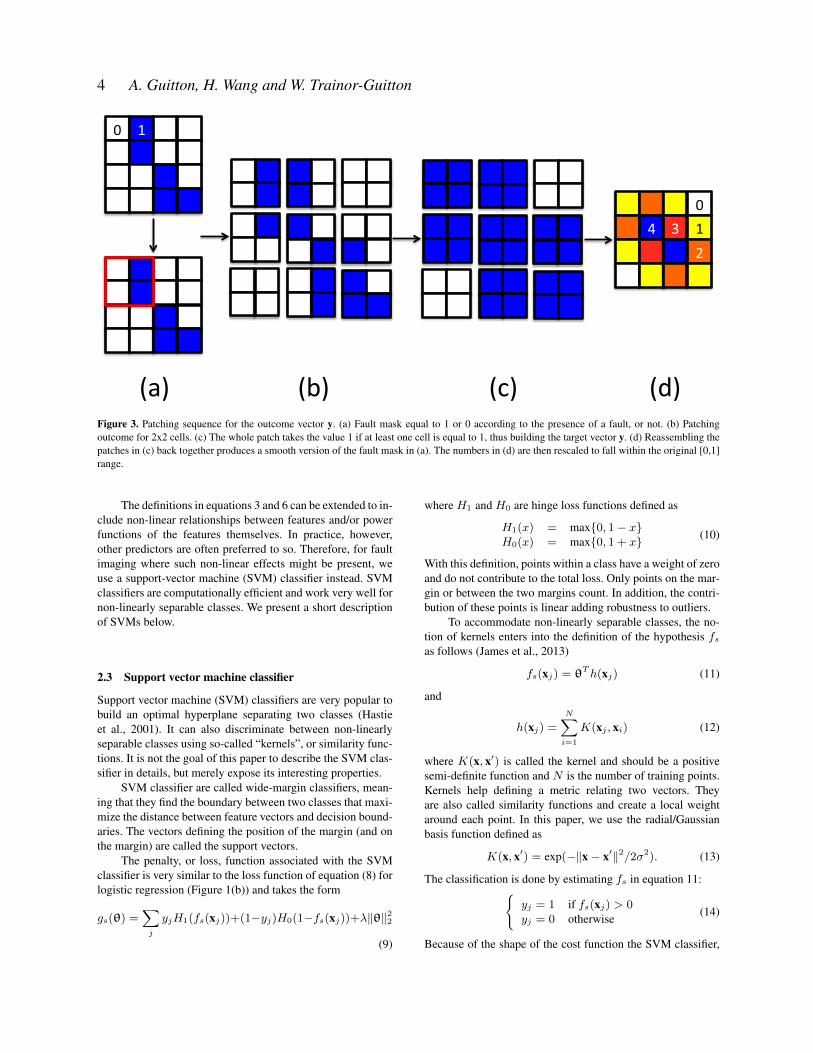
(a) (b) (c) (d)Figure 3. Patching sequence for the outcome vector y. (a) Fault mask equal to 1 or 0 according to the presence of a fault, or not. (b) Patchingoutcome for 2x2 cells. (c) The whole patch takes the value 1 if at least one cell is equal to 1, thus building the target vector y. (d) Reassembling thepatches in (c) back together produces a smooth version of the fault mask in (a). The numbers in (d) are then rescaled to fall within the original [0,1]range.

The definitions in equations 3 and 6 can be extended to in-clude non-linear relationships between features and/or powerfunctions of the features themselves. In practice, however,other predictors are often preferred to so. Therefore, for faultimaging where such non-linear effects might be present, weuse a support-vector machine (SVM) classifier instead. SVMclassifiers are computationally efficient and work very well fornon-linearly separable classes. We present a short descriptionof SVMs below.

2.3 Support vector machine classifier

Support vector machine (SVM) classifiers are very popular tobuild an optimal hyperplane separating two classes (Hastieet al., 2001). It can also discriminate between non-linearlyseparable classes using so-called “kernels”, or similarity func-tions. It is not the goal of this paper to describe the SVM clas-sifier in details, but merely expose its interesting properties.

SVM classifier are called wide-margin classifiers, mean-ing that they find the boundary between two classes that maxi-mize the distance between feature vectors and decision bound-aries. The vectors defining the position of the margin (and onthe margin) are called the support vectors.

The penalty, or loss, function associated with the SVMclassifier is very similar to the loss function of equation (8) forlogistic regression (Figure 1(b)) and takes the form

gs(θ) =∑j

yjH1(fs(xj))+(1−yj)H0(1−fs(xj))+λ‖θ‖22

(9)

where H1 and H0 are hinge loss functions defined as

H1(x) = max{0, 1− x}H0(x) = max{0, 1 + x} (10)

With this definition, points within a class have a weight of zeroand do not contribute to the total loss. Only points on the mar-gin or between the two margins count. In addition, the contri-bution of these points is linear adding robustness to outliers.

To accommodate non-linearly separable classes, the no-tion of kernels enters into the definition of the hypothesis fsas follows (James et al., 2013)

fs(xj) = θTh(xj) (11)

and

h(xj) =

N∑i=1

K(xj , xi) (12)

where K(x, x′) is called the kernel and should be a positivesemi-definite function and N is the number of training points.Kernels help defining a metric relating two vectors. Theyare also called similarity functions and create a local weightaround each point. In this paper, we use the radial/Gaussianbasis function defined as

K(x, x′) = exp(−‖x− x′‖2/2σ2). (13)

The classification is done by estimating fs in equation 11:{yj = 1 if fs(xj) > 0yj = 0 otherwise

(14)

Because of the shape of the cost function the SVM classifier,


contrary to logistic regression, doesn’t provide classes proba-bilities.

Training an SVM classifier requires parameters tuning.The first parameter λ decides how flexible (or how biased) wewant the classifier to be. Having a very large λ value yields ahigh bias/low variance classifier. A low value of λ yields theopposite. This value is related to as how many misclassifica-tions (or how wide the margin) are we allowing: a wide margin(large λ) means many vectors can be on the wrong side of theboundary decision. The second parameter comes from the ker-nel definition. A discussion regarding the choice of kernel goesbeyond the scope of this paper but in our selected radial basisfunction, we have to pick the variance σ2. There again, a verywide Gaussian function means higher bias and lower variance,while a small value of σ2 means the opposite.

In practice, we select the value of σ2 and λ by estimatingmany SVM classifiers for a wide range of values of σ2 and λ(e.g., [10−5, 105]) and select the values that yield the lowestclassification error. Statistically, we perform cross-validationusing a dataset called the validation set, different from thetraining or test sets (see details below).

The SVM classifier is quite similar to logistic regression,as exemplified in the similarities between the two loss func-tions of Figures 1(b) and 1(a). SVM has a computational edgeover logistic regression because only observations within themargins or at the margins matter. Note that kernels could alsobe easily incorporated into the definitions of logistic regressionbut without the same computational benefits.

It is interesting to see that a trend using neural networks(NNs) is re-emerging for the interpretation of seismic data(Araya-Polo et al., 2017; Huang et al., 2017). The fact thatNNs can be efficiently trained and optimized on hardware ac-celerators such as GPUs seems to be the most compelling rea-son why they are being used. However, NNs are also quiteexpensive to train. We think that determining the right featuresets for the training of the classifier is one of the most im-portant element of MLAs and will benefit any classifier. Fur-thermore, the right set of features might save us from usingvery expensive classifiers such as NNs while still obtainingsatisfying prediction results. Therefore, we think that SVMswith the appropriate kernels and parameterization combinedwith meaningful features should yield accurate-enough faultimages. Testing other classifiers such as NNs will come at alater time.

Having introduced the classifier, we now describe the fea-ture sets used for the fault imaging problem.

3 FEATURES COMPUTATION FOR FAULTDETECTION

The classifier is only one component of the whole MLA: ithelps us deciding whether a training point belongs to a classor another. The next vital component of the MLA is the featureset: what feature in the seismic image are we going to use tomake the classification easier?

The most simple feature is the seismic data itself, usingamplitude information only. Unfortunately, amplitude is a very

poor predictor of faults in seismic data and we need to find bet-ter attributes to characterize them. Measures of continuity inseismic data make better predictors, such as semblance. How-ever here, we opted for two classes of features that are widelyused in computer vision for object recognition. One is calledScale Invariant Feature Transform (SIFT) (Lowe, 1999), andthe other one is called Histogram of Oriented Gradients (HOG)(Dalal and Triggs, 2005). These two methods yield sets of fea-tures that can be used for classification. One of their biggestshortcoming is that they work in 2D slices only: we know thatadding more dimensions to the fault detection problem yieldsbetter results. One could expend these methods to extract 3Dattributes, however.

We are now going to briefly review the SIFT and HOGalgorithms.

3.1 Histogram of Oriented Gradients

The computation of HOG features is quite simple and compu-tationally efficient (Dalal and Triggs, 2005). First, an image isdecomposed into cells and blocks. Cells are usually half thesize (in number of pixels) of blocks. Blocks are mostly usedfor normalization purposes of the histograms. In general, butnot always, cells are 8x8 and blocks 16x16.

The first step consists in computing vertical ∇z and hor-izontal ∇x gradients using centered 1D derivative operators[−1, 0, 1] at each location in the image. From these gradients,signed (between 0o−360o) and unsigned (between 0o−180o)angles are computed (e.g. α = atan(∇z/∇x)).

Next, histograms of angles are computed for each cell.In practice, nine orientations bins are usually estimated, whereeach angle is linearly interpolated between neighboring bins.The value of the bin depends on the gradient magnitude (∇2

x+∇2

z)0.5

Note that it would be possible to extend these compu-tations to 3D by estimating histograms of oriented dips andazimuths (Marfurt, 2006). For dips, we could compute

α = atan

((∇2

x +∇2y)

1/2

∇z

), (15)

and for azimuth

ψ = atan2(∇x,∇y). (16)

Incorporating 3D attributes like these will help the classifica-tion and should be explored further.

Once histograms have been estimated, a normalizationstep follows. The normalization compensates for local varia-tions in amplitudes due to illumination effects, noise, geologyetc... The normalization is done for each block (i.e., groups ofcells) where blocks are overlapped. For each block, a normal-ization factor is computed as follows: if v is the unnormal-ized vector of all histogram values for all cells belonging to ablock, compute the normalization factor

√‖v‖22 + ε, where ε

is a constant to be chosen (with little impact on the classifica-tion results). Each histogram within a block is then normalizedby this value.

This completes the computation of HOG features. Again,


Figure 4. (a) A window extracted from a 2D slice after patching. (b) Illustration of SIFT features extracted from (a): 15 keypoints were identifiedwith different orientations. (c) Illustration of the HOG features extracted from (a): histograms are represented as rose diagrams.

the 3D extension should be easily doable and investigated fur-ther. We now look at the Scale Invariant Feature Transform(SIFT).

3.2 Scale Invariant Feature Transform

SIFT is another popular descriptor for image classification.The goal of SIFT is to match features across different images.The power of SIFT is that it can match features between im-ages that are rotated, scaled (size-wise), illuminated or viewedfrom different angles. The computation of SIFT descriptors ismore involved than for the HOG ones. We will focus on themain steps only.

The first step of SIFT consists in finding keypoints in theimage. These keypoints are supposed to represent prominentfeatures in the image. Finding these keypoints requires manysteps. First, the image is transformed into a scale space: the im-age is simultaneously blurred with different Gaussian kernelsand sub-sampled (halved between scales). Each scale is calledan “octave”. Therefore, after this first stage, SIFT creates manyduplicates of the image at different scales (i.e., resolution) andwith different smoothing functions. In other words from oneimage, we end up with many cubes of different sizes whereeach panel of a cube has a different blurring kernel appliedto it. Then, for each octave, two consecutive blurred imagesare subtracted to create a Difference of Gaussians (DoG) scalespace. In the next step, local extrema (minima and maxima)are detected by looping over all pixels for each scale withinan octave and comparing it with its closest 26 neighbors (apixel has 26 neighbors in a cube). The local extrema are thenquadratically interpolated so that we have a value of extremaeverywhere. It is recommended to have two such images of

extrema per octave, which means four DoG images per octaveand five blurring kernels. Extrema with low contrast responsesand close to the edges are discarded.

Once the keypoints are identified at different scales, anorientation for each keypoint is estimated. To do this, a localdip is estimated for all points surrounding a keypoint usingthe same formula as the one used for the HOG method. Thena histogram of all dip values is computed. The bin with thehighest value is assigned as the keypoint dip. Other keypointswith the same location and scale are created for all bins within80% of the highest value.

Finally, for each keypoint 16 blocks (4x4) are definedwith 16 pixels per block (4x4). Within each block, histogramsof gradient magnitudes and orientations are computed andbinned in an 8 bins histogram (similar to HOG). The keypointorientation is subtracted from all computed orientations withinsurrounding blocks to preserve rotation independence. The binvalues are also clipped for normalization. Therefore, for eachkeypoint, we have a vector of 128 descriptors (16 blocks times8 bins). For classification, the descriptor of 128 elements isused rather than its location.

Some of the major differences between the HOG andSIFT descriptors are the scale invariance property built in theSIFT, not present in HOG, and the selection of keypoints. Foreach image, the number of keypoints will be different andmore steps are needed to use the SIFT descriptor with MLA.We detail these steps below.

3.3 Clustering of SIFT features

From the description of the SIFT descriptor above, it is clearthat different images will have a different number of keypoints.


This is problematic with MLAs because we want the size ofthe feature vector to be the same for each data point.

To remedy the fact that the number of keypoints will bedifferent for different images, we first estimate the SIFT fea-tures for each training image. For each image i, we end upwith a descriptor D128×Mi where Mi is the number of key-points for image i and 128 is the number of orientation bins(8) times the number of blocks (16) surrounding the keypoint.Then, we pack all the descriptors for all images into one largematrix D of size 128×

∑iMi.

The matrix D contains all vectors of size 128 for alltraining images. In the next step, we classify the vectors us-ing K-means clustering, an unsupervised learning algorithm.The number of centroids doesn’t need to be large. For the faultdetection problem, 20 centroids seem to be enough. Once thecentroids in the 128 dimensional space are found, we classifyall descriptors for all images into the 20 classes (using small-est distance). If, for one image, l descriptors fall into one class,the class takes the value l. We end up for each image with ahistogram of centroid values that has the same size for all im-ages. If no keypoint is found in one image, then the histogramis zero for all 20 bins. Another advantage of this process is thatit reduces the size of the feature vector considerably (only 20elements in our case).

The workflow is now almost complete. We compute HOGand SIFT features from seismic images. SIFT features are sim-plified by clustering. The features are fed into an SVM clas-sifier for training. The SVM classifier is then used for classi-fication. Now, we present our workflow for the fault detectionproblem first with 3D synthetic data, then with 3D field data.

4 3D STATISTICAL FAULT DETECTION WITHSYNTHETIC DATA

The proper training, parameterization and execution of anMLA requires validation, training, and test sets. These threesets are mutually exclusives and don’t contain the same datapoints. For seismic interpretation, we have enough data toproperly build these easily. The MLA is trained on the trainingdataset and its parameterization is tested on the validation set.For the SVM classifier with a Gaussian kernel, two parametersare estimated with 5-fold cross-validation: σ (equation 13) andλ (equation 9). Once the parameters are estimated, the trainingis performed using the training set and the classifier is appliedto the test set.

4.1 Building the outcome vector

For the fault imaging problem, we first need to buildthe required sets of labeled seismic data. For this, webuild many synthetic datasets with different fault geome-tries (normal, conical, conjugate) and pick them using theMines Java Toolkit (https://github.com/dhale/jtk) and theseismic image processing for geological faults software(https://github.com/dhale/ipf). The fault picking part is ex-plained in details in Hale (2013). For the training and valida-

tion sets, we use the volumes in Figures 2(a), 2(b) and 2(c). Webuild the features vectors xj from the seismic volumes and theoutcome vector y from the fault picks. We now explain howthese features are extracted.

4.2 Building the feature vectors

The HOG and SIFT features need to be estimated on smallwindows. Therefore, we decompose each cubes into 2D slicesalong the crossline direction. Each slice is then decomposedinto overlapping windows of 8x6 pixels, with an overlap zoneof half the window length in both directions. We estimate theHOG and SIFT features from these small windows. In thisparameterization, each patch (or window) becomes one train-ing/validation point.

For the outcome vector, we follow the same idea. Figure3 shows how the patching is done when the window size is2x2 (for illustration purposes only). In Figure 3a, we have amasking function equal to 1 or 0 when a fault is present ornot. In Figure 3b, patches of size 2x2 are formed. If a faultis contained in a patch, we assign the value 1 to the wholewindow, 0 otherwise (Figure 3c): this last step gives us theoutcome vector for each patch. Going backward, reassemblingthe patches back to the original grid, we end up with Figure 3d:due to the patch size and overlap, the fault location is smoothedacross the 2D slice as shown by the numbers in the cells (inpractice, the cells are then re-normalized so that the maximumvalue is one).

From the patching of the 2D seismic slices, we extract theindividual windows and estimate the HOG and SIFT features.Figure 4 illustrates these features. Figure 4a shows a patch ofsize 8x6. From this patch SIFT features are extracted and dis-played in Figure 4b. For this window, 15 keypoints are iden-tified, corresponding to 15 circles. The size of the circle cor-responds to the scale, or octave, the feature was identified in.The bars correspond to the orientations picked at the keypointlocations. Other windows will have different number of key-points, orientations and circle sizes (i.e., scale). The clusteringalgorithm presented above remedies this issue and providesus with 20 features for all points. The HOG features are dis-played in figure 4c. The histograms of oriented gradients arerepresented as rose diagrams. When slopes are locally consis-tent, the histogram is very narrow and highlights a fairly uni-form direction. For each window (patch), 12 histograms areestimated for a total of 768 features.

From 3D volumes of interpreted faults and seismic data,we build 2D patches. Each patch makes up for one data point.From the fault mask patches, we build the outcome vector y.From the seismic data patches, we build the feature vectors xj

using HOG and SIFT algorithms. The final size of each featurevector is 788 (768 from HOG, 20 from the clustering of theSIFT vectors). With all our labeled data and features sets avail-able, the training of the SVM classifier can start. In the nextsections, we show our training/prediction results with differentcombinations of features (HOG vs. SIFT vs. HOG+SIFT).


Figure 5. Test data with its interpreted faults. This dataset comprises conical, conjugate and normal faults. These data are not used for training orcross-validation.

(a) (b)

Figure 6. Confusion matrices for (a) the training data and (b) the test data when the HOG features only are used. The error rate for the trainingdata is very low at 0.6% (bottom right blue corner). The error rate for the test data is higher, as expected, at 7.9%. Looking more closely at thesecond row of (b), we notice that our classifier tends to overpredict faults, with an error rate of 20.8% (meaning that 20.8% of predicted faults arenot faults).

4.3 Fault interpretation with HOG features only

We first train and predict using the HOG features only. Thetraining is done using the seismic volumes in Figures 2(a), 2(b)and 2(c). After patching, 600,000 windows are available forvalidation and training. We extract randomly 40,000 patchesfor training and 7,500 for validation (i.e. parameterization ofthe SVM classifier with Gaussian kernels).

The training outcome is displayed in the confusion matrixof Figure 6(a). The confusion matrix summarizes the train-ing error by displaying the true/false positive/negative ratios.

The diagonal elements show the true positive and true nega-tive rates. The off-diagonal elements show the false positiveand false negative rates (classification errors). The bottom rowand right-most column show a summary (in percentage) of theclassification errors/successes. The bottom right corner (blue)shows in green the total success rate (sum of diagonal ele-ments) and in red the total misclassification rate (sum of off-diagonal elements). The training here is very good, with a verylow classification error. Only 245 patches with faults were mis-classified as not having faults, while only 2 patches withoutfaults were misclassified as having faults. Such a low error


(a) (b)

(c) (d)

Figure 7. (a) True fault locations after reassembling the patches (and thus smoother than in Figure 5) and (b) predicted faults locations for the testdata when HOG features are used only. The prediction highlights the faults accurately with some edge effects. (c) Predicted fault locations for thetest data when SIFT features are used only. The prediction is quite noisy and not as accurate as in Figure 7(b). (d) Predicted fault locations for thetest data when HOG and SIFT features are used. The prediction is cleaner than in Figure 7(b) with fewer misinterpreted faults on the edges of thecube.

rate might indicate an overfitting of the training data which wecould remedy by adding more training data.

After training, we use the SVM classifier to identify faultsin a seismic volume not seen during training or validation (Fig-ure 5). We use 200,000 windows for the test data. Figure 6(b)shows the confusion matrix for the test data. The classificationerror increases significantly, as expected. Looking at the sec-ond row of the confusion matrix, we notice that 20% of theinterpreted faults are misclassified. Looking at the first row,only 4.5% of the non-faults are misclassified. Therefore, ourclassifier tends to over-predict faults.

Figure 7(a) shows the interpreted faults after reassem-bling the patches of the faults images in Figure 5. The patch-ing makes the faults wider, as already explained in Figure 3.

We consider Figure 7(a) to be the answer, or true prediction,of the fault locations. Figure 7(b) displays the locations ofour predicted faults using the HOG features only. There is avery good agreement between Figures 7(a) and 7(b). We no-tice some edge effects that would be mitigated with a propertaper function. Overall, the classifier was able to identify allfaults properly. Given that the feature vector is computed on2D windows only, we think that better results would be possi-ble by estimating features in 3D. Yet, the classifier performedremarkably well.


(a) (b)

Figure 8. Confusion matrices for (a) the training data and (b) the test data when the HOG and SIFT features are used. The error rate for the trainingdata has increased to 8.5% (bottom rights blue corner). Looking more closely at the second row of (b), we notice that our classifier tends to predictfewer faults than in Figure 6(b) with a lower error rate of 18.1%. Predicting fewer faults translates into a cleaner image.

4.4 Fault interpretation with SIFT features only

Now we train our SVM classifier using the SIFT features only.For this case, we show the classification results only in Fig-ure 7(c). Clearly, the classification error is high. Although notshown here, the confusion matrix indicates that 37% of faultsin Figure 7(c) are misclassified. Increasing the number of cen-troids in the clustering part of the SIFT vectors didn’t changethis rate.

4.5 Fault interpretation with HOG and SIFT features

We are now combining HOG and SIFT features to train ourclassifier. The classification result is shown in Figure 7(d) andseems to indicate a better classification than when HOG fea-tures are used only. Looking at the confusion matrices for thetraining and test data in Figures 8(a) and 8(b), we notice thatthe overall training error has increased to 8.5% compared tothe 0.6% seen Figure 6(a). However, the test error has re-mained pretty constant. Using HOG and SIFT features hasreduced the variance of our classifier, decreased the misclassi-fications of faults by 2%, and increased the misclassificationsof no-faults by 2% as well (precision has increased, recall hasdecreased). In other words, our prediction has become moreconservative and has predicted fewer faults (42326 with HOGonly, 36908 with HOG and SIFT), thus resulting in a cleanerimage. Because of the overlap of the patches and the inher-ent robustness coming with it (the information for one fault isspread among many patches), missing more faults is beneficialto the overall prediction.

Therefore, although counter-intuitive given the numbersin the confusion matrices, combining HOG and SIFT featuresfor the fault imaging problem yields the best results. Better

classification results could be obtained if more training datawere added: we are only using 40,000 points out of 600,000 tolimit the computing cost of the training part.

In the next section, we use our approach to image faultsfor a 3D field data example where many faults are present.

5 3D STATISTICAL FAULT DETECTION WITHFIELD DATA

Field data are more challenging than synthetic data. Buildingsynthetic training data and applying them to field data mightnot be the best approach because we might not capture thecomplexity of faults in 3D with simple models. It seems a bet-ter approach to train the classifier with field data examples aswell. Ideally, we would want to access lots of labeled seismiccubes with different fault geometries, different noise levels,different geological settings, etc... The classifier, similar to ahuman interpreter, would learn from all these scenarios andwould improve its predictions.

For the field data example therein, we select a small 3Dseismic volume instead that we divide in three parts for vali-dation, training and testing. We follow the same procedures aswith the synthetic data with two important differences. First,the window size for each patch is now 8x12, as opposed to8x6 for the synthetic dataset. Finally, a patch has a fault if atleast 16 cells in the patch (out of a possible 96) have the faultmarker set to one. By limiting the number of patches gettingthe value y = 1, we make our classifier more robust to noise.For the validation step, we use 30,000 points. For the trainingstep, we use 128,000 points. For the testing, we use 147,000points.

Figure 11(a) shows the test data, not seen by the classi-


fier, and Figure 11(b) displays the labeled faults using Hale’ssoftware (and after reassembling the outcome vector patches).Using field data presents an interesting challenge, beyond thenoise problem mentioned above. The labeling of the faultsis indeed not accurate everywhere. Looking at Figure 11(b)we see fault locations in the test data not picked by the au-tomated fault detection software. It might also happens thatpicked faults are not true faults. Therefore, the training of theclassifier is done with mislabeled data, where false positivesand false negatives are present.

We train the SVM with the HOG features only. The con-fusion matrix for the training part is shown in Figure 9(a). Theoverall training performance is excellent, with a near-perfectprediction. This indicates an overfit of the training data whichoften results in a poor performance of the classifier on testdata. This can be seen Figure 9(b) where the classification ofthe test data is indeed less accurate (77%). The outcome vectorfor the test data mapped back into the original dataset space isshown in Figure 11(c). To increase the vertical and horizontalcontinuity of faults in the crossline direction, we smooth thefault map of Figure 11(c) and obtain Figure 11(e). It is pleas-ing to see that the five major vertical faults between x=609 kmand x=613 km are identified by the classifier. Their lateral ex-tent in the crossline direction is also clearly predicted by theMLA.

Now, we train the SVM with both HOG and SIFT fea-tures. Figure 10(a) shows the confusion matrix for the train-ing part. Adding the SIFT features clearly affects the perfor-mances of the training part, with a 86.5% success rate. Thisis a well-known effect of adding more features to the train-ing of any classifier. Similar to the synthetic experiment, Fig-ure 10(b) shows that adding the SIFT features increases theprecision by 4%, which is significant: we are predicting lessfaults but more accurately. Next, we map the predicted out-comes back into the seismic volume in Figure 11(d). We no-tice that the main faults are predicted correctly. We can also seethat we are missing some faults, comparing with Figure 11(b),but that we are also picking real faults not visible in Figure11(b). Therefore, our MLA does better in some areas, worsein others. Finally, to improve the continuity of faults in the ver-tical and crossline directions, we apply a small smoothing tothe predicted faults (Figure 11(f)). The smoothing makes for amore realistic fault image. This process should be incorporatedsomehow inside our training part.

6 DISCUSSION

Overall, our approach to predict fault locations using MLAworks. We label faults using an automated procedure devel-oped by Hale. We build feature vectors using standard objectrecognition methods such as HOG and SIFT. We use an SVMclassifier with Gaussian kernels. There are many avenues forimprovement, however.

From a MLA view point, we could improve our predic-tion by incorporating some smoothness in the predictor di-rectly and not in a post-processing step. For this, the method of

Wang et al. (2014) using spatially-temporally consistent ten-sors could be used. In the geophysical world, this comes downto adding a smoothness term to the fitting goal. Another im-provement could come by integrating all our features (SIFTand HOG) in a better way by adding a joint-structured sparsityregularization term (Wang et al., 2013). In essence, we cantry to identify automatically the best features for all vectors.Finally, we could use a semi-supervised approach where wedon’t label all faults but just a few: this would save time andmight handle the mislabeling issue with field data better.

From a feature computation view point, extending theSIFT and HOG methods to 3D is the next natural step. Whilethe labelling is done in 3D, the features are estimated in 2Dplanes only. By taking the SIFT and HOG features to higherdimensions, better predictions would follow. In addition, wecould use other features such as semblance, dip, etc... for theclassification. However, it is quite remarkable that standard ob-ject recognition techniques work so well with seismic data.

Additionaly, we need to include more training data tohave a classifier able to identify faults in many environments.Increasing the size of the training data requires larger comput-ing cappabilities and more efforts have to be made to optimizethe computation of both features and predictor. To this end,being able to run these algorithms efficiently on GPUs will berequired.

Finally, the fault imaging problem is only one possibleapplication of MLAs with seismic data. Other features suchas channels or sequence boundaries can be included as well.MLAs can also be very useful in the integration of many datatypes where the volume and complex interaction between themmakes it hard to do with standard inversion approaches.

7 CONCLUSION

We highlight faults in 3D seismic volumes using a supervisedmachine-learning approach. We label faults using an auto-mated fault-picking method developed by Hale. We build fea-ture vectors using two methods widely used in object recogni-tion techniques called HOG and SIFT. We use a standard SVMclassifier with Gaussian kernels for our predictor. On both 3Dsynthetic and field data examples, we show that a combinationof HOG and SIFT features yields better classification results:the precision increases resulting in a lower false-positive rate.We also demonstrate that a non-accurate labelling of the train-ing data doesn’t necessarily prevent the MLA from predictingfaults: this is an important message with field data where mis-labelling will occur. Finally, we prove that although not opti-mal, features extracted in 2D can still be useful in 3D contexts.However, we advocate to extend HOG and SIFT to 3D thusyielding better classification results.

REFERENCES

Araya-Polo, M., T. Dahlke, C. Frogner, C. Zhang, T. Pog-gio, and D. Hohl, 2017, Automated fault detection withoutseismic processing: The Leading Edge, 36, 208–214.


(a) (b)

Figure 9. (a) Confusion matrix for the field training data using the HOG features only. The near-perfect training result indicates an overfit of thetraining data. This often results in poor performance of the classifier on test data. (b) Confusion matrix for the field test data. More realistic numbersare obtained: 77% of data are classified correctly. The precision is around 52%.

(a) (b)

Figure 10. (a) Confusion matrix for the field training data using the HOG and SIFT features. 61% of “true” faults (target) are not labeled correctly.(b) Confusion matrix for the field test data. Similar to the synthetic case, adding more features increases the precision. The classifier has lessvariance.

Dalal, N., and B. Triggs, 2005, Histograms of oriented gra-dients for human detection: Proceedings of the 2005 IEEEComputer Society Conference on Computer Vision and Pat-tern Recognition (CVPR’05) - Volume 1 - Volume 01, IEEEComputer Society, 886–893.

Hale, D., 2013, Methods to compute fault images, extractfault surfaces, and estimate fault throws from 3d seismicimages: Geophysics, 78, O33–O43.

Hastie, T., R. Tibshirani, and J. Friedman, 2001, The Ele-ments of Stastical Learning, Data Mining, Inference, andPrediction: Springer.

Huang, L., X. Dong, and T. E. Clee, 2017, A scalable deeplearning platform for identifying geologic features fromseismic attributes: The Leading Edge, 36, 249–256.

James, G., D. Witten, T. Hastie, and R. Tibshirani, 2013, AnIntroduction to Statistical Learning, with Applications in R:


(a) (b)

(c) (d)

(e) (f)

Figure 11. (a) Test data. (b) Fault images picked automatically. Predicted faults using (c) HOG features and (d) HOG+SIFT features. Predictedfaults after smoothing for (e) HOG features and (f) HOG+SIFT features. The color scale goes from 0 (green) to 1 (red) and could be interpreted asa fault probability map. Smoothing improves temporal and spatial continuity.


Springer.Lomask, J., A. Guitton, S. Fomel, J. Claerbout, and A. A.

Valenciano, 2006, Flattening without picking: Geophysics,71, P13–P20.

Lowe, D. G., 1999, Object recognition from local scale-invariant features: Proceedings of the Seventh IEEE Inter-national Conference on Computer Vision, 1150–1157 vol.2.

Marfurt, K. J., 2006, Robust estimates of 3D reflector dip andazimuth: Geophysics, 71, P29–P40.

Marfurt, K. J., R. L. Kirlin, S. L. Farmer, and M. S. Bahorich,1998, 3-D seismic attributes using a semblance-based co-herency algorithm: Geophysics, 63, 1150–1165.

Pedersen, S. I., T. Skov, T. Randen, and L. Sønneland, 2005,Automatic fault extraction using artificial ants: in Math-ematical Methods and Modelling in Hydrocarbon Explo-ration and Production, Springer Berlin Heidelberg, 107–116.

Stark, T. J., 2004, Relative geologic time (age) volumes-relating every seismic sample to a geologically reasonablehorizon: The Leading Edge, 23, 928–932.

Wang, H., F. Nie, and H. Huang, 2014, Low-rank tensor com-pletion with spatio-temporal consistency: Proceedings ofthe Twenty-Eighth AAAI Conference on Artificial Intelli-gence, AAAI Press, 2846–2852.

Wang, H., F. Nie, H. Huang, and C. Ding, 2013, Hetero-geneous visual features fusion via sparse multimodal ma-chine: 2013 IEEE Conference on Computer Vision and Pat-tern Recognition, 3097–3102.

statistical identiﬁcation of faults in 3d seismic volumes using a ... · 4 a. guitton, h. wang...

Documents