Statistical Estuary Data Analysis in Models and Measurements – Some Methods and their Limitations

Marko Kastens

Summary

This paper considers the impact of people on a complex natural system like an estuary and how this influence can be assessed. The methods of mathematical modelling and analysis of measured data are briefly introduced and their advantages and shortcomings highlighted. The paper looks into statistical methods for time series analysis, using the example of the water level - a parameter that represents a mixed times series signal consisting of harmonic and non-harmonic components. Some spectral methods and the regression method are then chosen from the wide selection of methods available and their limitations and prerequisites are discussed. A procedure combining both methods is presented and applied to the example of the Elbe gauge in Hamburg-St. Pauli. The focus is on the method and its limitations; the results obtained are of secondary importance and are not discussed here. Reference is made to a relatively recent method of analysing non-stationary and nonlinear phenomena (Hilbert Huang Transform). The application of this method would, however, imply abandoning the classical view of the tidal wave as consist-ing of partial tides. Since it is hardly possible any more for one single person or institution to be familiar with the vast selection of analytical methods or to apply them, the analysis of and research into complex systems will require cooperative approaches in the future.

Keywords

statistical methods, regression method, spectral methods, FFT, LSSA, wavelet analysis, neural networks, water level development, estuary, Elbe, Hamburg-St. Pauli

Zusammenfassung

Anhand der Leitfrage, wie der Einfluss des Menschen auf ein komplexes natürliches System, wie dem Ästuar, beurteilt werden kann, werden die Methoden der mathematischen Modellierung und der Messda-tenanalyse mit ihren Vor- und Nachteilen kurz dargestellt. Anhand des Parameters Wasserstand, der stellvertretend für ein aus harmonischen und nicht harmonischen Anteilen gemischtes Zeitreihensignal steht, werden statistische Methoden zur Zeitreihenanalyse behandelt. Aus der Fülle der Methoden werden einige Spektralmethoden und das Regressionsverfahren ausgewählt und ihre Limitierungen und Voraus-setzungen besprochen. Ein aus beiden Methoden kombiniertes Verfahren wird vorgestellt und am Beispiel des Elbepegel Hamburg-St. Pauli angewendet. Im Vordergrund steht die Methode mit ihrer Begrenzung; die Ergebnisse sind sekundär und werden nicht weiter diskutiert. Eine relativ neue Analysemethode für nichtstationäre und nichtlineare Phänomene wird erwähnt (Hilbert-Huang-Transformation), die jedoch

185

Die Küste, 81 (2014), 185-201

die Aufgabe der klassischen Sicht der Tidewelle bestehend aus Partialtiden bedeutet. Die Fülle und Breite der vorhandenen Analysemethoden, die weder ein Mensch noch eine Institution kaum mehr über-blicken oder anwenden kann, fordert zukünftig ein kooperatives Vorgehen in der Analyse und Erforschung komplexer Systeme.

Schlagwörter

Statistische Methoden, Regressionsverfahren, Spektrale Methoden, FFT, LSSA, Waveletanalyse, Neuronale Netze, Wasserstandsentwicklung, Ästuar, Elbe, Hamburg-St. Pauli

Contents

1 Introduction ...................................................................................................................... 186

1.1 Numerical simulation model: ......................................................................................... 187

1.2 Analysis of data gathered in field measurements: ....................................................... 187

2 Analysis of model results ................................................................................................ 188

3 Analysis of field measurements ..................................................................................... 188

4 The water level as the lead parameter ........................................................................... 189

5 Methods of time series analysis ..................................................................................... 189

5.1 Harmonic analysis ............................................................................................................ 190

5.1.1 Fast Fourier Transform (FFT): ............................................................................ 190

5.1.2 Least-squares spectral analysis (LSSA): .............................................................. 194

5.1.3 Wavelet analysis ...................................................................................................... 195

5.2 Regression analysis ........................................................................................................... 195

5.2.1 Results ...................................................................................................................... 197

5.2.2 Evaluation of the results ....................................................................................... 198

5.3 Neural networks ............................................................................................................... 199

5.4 Other methods ................................................................................................................. 199

6 Conclusion ......................................................................................................................... 200

7 References ......................................................................................................................... 200

1 Introduction

The key question addressed in this paper is: How can we assess or, even better, quantify the past, current and future influence of humans on a natural system like an estuary? To answer this question, the system investigated (the estuary in this case) must be under-stood as comprehensively as possible.

An estuary is a highly dynamic and complex system, which is explained at length in the extensive literature, for example PUGH (2004), NIELSEN (2009) or MALCHEREK (2010)). It reacts time and again not only to external influences such as flood waves from upstream or changes in the sea connected to the estuary but also to human influence, and it is subject to permanent alteration and adaptation. It is of interest to understand how

186

Die Küste, 81 (2014), 185-201

phenomena such as the increase in the tidal range can be ascribed to certain events both regarding their cause and in quantitative terms?

Applying the following two methods helps - at least to some degree - to answer these questions. The first method is the numerical simulation model. Based on the relevant physical laws it endeavours to simulate estuarine dynamics on the computer. The second method is the analysis of data gathered in field measurements. Both methods come with their own major advantages and considerable deficiencies which are listed below.

1.1 Numerical simulation model:

+ is an internally consistent system which enables the user to vary just one parame-ter and observe the impact of the alteration on the overall system (system studies).

+ enables predictions about the system behaviour following complex changes of in-itial and boundary values.

+ provides a comprehensive view of the overall estuarine system. - maps natural processes only in an incomplete, model-based way. This results in in-

accuracies in the calculations and related conclusions. - uses a discretisation and parameters adjusted to the former. If the discretisation is

increased, which is in most cases due to a desire to reduce the inaccuracies, the two scales may no longer fit together (up-/downscaling) so that the effort of recalibrating the model is necessary. This requires considerable experience, knowledge and depending on the circumstances, also a lot of time.

- always uses initial values (e.g. sediment covering of the bed) and boundary values (e.g. the water level at the seaward edge). These values are incomplete and/or in-accurate, which can also lead to increased inaccuracies in the calculations and predictions.

1.2 Analysis of data gathered in field measurements:

+ is based on reality. By contrast, model conditions are either purely hypothetical or they are hindcasts or nowcasts with the above mentioned inaccuracies.

- is characterised by some inaccuracies in the measured values. - may have gaps due to the failure of measurement equipment or other adversities,

resulting in time periods for which no data is available. - is often limited to individual spots. Since spatial representativeness has to be

estimated, the informative value of field measurements has its limitations in many cases.

- fails to distinguish between natural and anthropogenic influences, but only shows changes.

- is incapable of providing forecasts. Extrapolating measurements into the future is only possible for short time periods and subject to uncertainties.

The above list of pros and cons shows that neither of the two methods is clearly superior to the other, but that their different perspectives rather complement each other and can open up a new dimension - as is the case with stereoscopic vision which requires two eyes.

187

Die Küste, 81 (2014), 185-201

The use of both methods depends on a fundamental understanding of the system. On the other hand, both methods can also enhance such understanding.

2 Analysis of model results

The overwhelming majority of mathematical simulation models yield large volumes of data which are then analysed, often with the aim of aggregating the data in order to reduce the data volume or elicit specific characteristics by which the model run can be distinguished from others. Generally speaking, this data constitutes characteristic numbers. The characteristic numbers are time and spatially referenced, in the latter in-stance to points, lines, surfaces and/or volumes, etc. Examples of such ratios are:

Events in a time series: tidal low water, tidal high water, slack tide (zero velocity), ... Statistical parameters: mean values, global minima and maxima, standard deviation,

variance Spectral characteristic numbers: amplitudes and phases of partial tides, spectrum of

sea waves, periodograms Integrative parameters: sums, partial sums and balances Differential parameters: velocities and accelerations (for morphological parameters

see MILBRADT (2011)) As many people find it easier to understand complex matters if they are represented by illustrations or animations, visualisation plays an important role in addition to these char-acteristic numbers.

A detailed description of the catalogue of characteristic numbers used by the BAW is provided in BAWiki (BAW 2014).

3 Analysis of field measurements

In principle, the aggregation examples listed above also apply to field measurements. However, preparing and harmonising the measurements requires significant additional work.

Preparing the measurements includes plausibility checks. Each measurement has to be verified, based on an individual error catalogue for the parameter (and for the measuring device, if necessary). If any errors are detected, the place affected must be marked, for example using a flag system. Some parameters will also need to be converted if the measurement relates to proxy information. The water level, for example, may be calculat-ed based on pressure measurements after making adjustments for the atmosphere. Or: sediment concentration which is derived from turbidity after calibration using measure-ment samples.

In the next step, the measuring data from different data sources (measuring devices, companies, authorities), including meta data, are converted to a standardised data format (ASCII, XML, NetCDF, …). Once the field data are harmonised and thus - in most cases - also standardised, they can be used for further analysis, although it is important to bear in mind that in contrast to model results measurements can have gaps because of missing data.

188

Die Küste, 81 (2014), 185-201

4 The water level as the lead parameter

After this general overview, a few methods of data analysis are employed in the following concrete examples. The parameter chosen as an example is the water level. Firstly, because it is an important lead parameter used in numerous environmental reports, and secondly because the German Federal Waterways and Shipping Administration (WSV) has been maintaining a gauge measurement network for many years - including databases and systems for storing and processing the data - so that at many gauges long time series are available which are sufficiently plausible and well documented.

The tidal Elbe and the gauge of Hamburg-St. Pauli which is located there, are used as the estuary example (for more information see Tide – Tidal River Development, EURO-PEAN UNION (2014)). In addition, to compensate for the external influence factors (dis-charge and sea) the gauges of Helgoland and Neu Darchau are used.

5 Methods of time series analysis

Many of the model results and field measurements are available as time series. Time series analysis is a tool used almost on a daily basis in a multitude of disciplines. It is numbered among the statistical methods which are used everywhere: from simple descriptive statis-tics (e.g. mean values) via probabilities (e.g. expected values and confidences) through to statistical tests and distributions, regressions and, last but not least, time series analysis, (e.g. HARTUNG et al. (2005)) a broad array of statistical methods for evaluating and de-scribing times series are available. Even spectral analysis may be considered a sub-field of statistics, although nowadays it tends to be regarded as a discipline in its own right. How-ever, as consideration of statistics in general would exceed the narrow bounds of this paper, the following discussion focuses on harmonic and regression analysis.

An analysis often starts with a phenomenology or qualitative analysis: What are the re-lationships between the parameters; are there any correlations and are they strengthened or weakened by other factors, etc. The next step is to perform a quantitative analysis. A qualitative analysis is the first step and precondition for regression which is described below. It requires a model function to describe the interaction of all parameters involved in a qualitative way. In the subsequent regression analysis, these parameters are deter-mined in quantitative terms.

Benchmarks are indispensable for verifying all the methods used. They enable verifica-tion of whether the respective method is suitable for the purpose of the analysis, which types of analysis may not work and what are the uncertainties inherent in the method. The time series analysis conducted here can be verified by a benchmark consisting of one or several completely artificial time series whose composition is 100 percent known (for example, the partial tides and their amplitudes and phases, the offset and, where applica-ble, the linear trend). When comparing the results obtained by different analysis methods, many insights can be gained as to whether or not a particular method is suitable for the purpose.

189

Die Küste, 81 (2014), 185-201

5.1 Harmonic analysis

The measurement of the water level in an estuary is influenced by the tide and by meteorological factors. The tides can be represented as partial tides with fixed frequen-cies. Each partial tide is a linear combination of the five basic frequencies of the sun-moon-earth system (e.g. GODIN (1988) and BAW (2007). Hence, a tidal signal must have a certain harmonic component.

Harmonic analysis of the water level has a long tradition (CARTWRIGHT 2000), where-as spectral methods have been applied in rather more recent studies. In the German literature examples of spectral analysis methods can be found in GÖNNERT et al. (2004) or LIEBIG (1994) who uses the method to close gaps in water level recordings.

In view of the extensive literature, no introduction to the methods is provided here. Instead, this paper focuses on the special aspects of employing these methods for the analysis of tidal signals. The preconditions, limitations and recommendations relating to some harmonic analysis methods are outlined in the following sections.

5.1.1 Fast Fourier Transform (FFT):

The Fast Fourier Transform (FFT) is a standard spectral analysis method. This widely used method and its application can be found in numerous textbooks and reference books (BUTZ (2003) and OPPENHEIM et al. (2004), to name but a few).

In a spectral representation, partial tides become visible in an amplitude spectrum as lines which clearly stand out from their environment (Fig. 1). Besides the harmonic component, which expresses itself in the dominating spectral lines, there is an aperiodic component. The latter moves roughly along a decreasing exponential function (red line). The major share of the aperiodic signal’s energy is located in the long-wave range (0 to 13 degrees/hour) before the first partial tide (Q1 in this case).

Figure 1: The beginning of an amplitude spectrum of a measured water level. The area of the mean water (0 to 13 degrees/hour) and several partial tides.

190

Die Küste, 81 (2014), 185-201

When applying FFT to analyse (tidal water level) time series, the following has to be taken into account: General statements

The signals caused by meteorological influences are mostly in the range of low fre-quencies (see Fig. 1). The influences decrease in power as the frequency increases. When considering the development of a spectrum over time, the peaks in the lower frequency band show variation, i.e. they are more of a stochastic nature. Partial tides form an almost constant peak in the amplitude spectrum over time.

A low-pass filter enables the main aperiodic portion of the signal to be separated from the rest of the signal. This portion represents a kind of baseline for the tidal signal and is referred to as mean water in this paper. The remaining signal portion corresponds to the main tidal signal which varies on the baseline. From a physical perspective the separation is not complete because meteorological influences lead to signals which are also in range of the frequencies of the partial tides; and: long-wave partial tides are superimposed by the meteorological noise in the range of 0 to 13 degrees/hour (e.g. the partial tides SA and SSA).

The fixed peaks in the amplitude spectrum allow the frequencies and thus partial tides to be determined. Peaks/partial tides that are not classified can be determined via a linear combination of the five astronomical basic frequencies.

Since the frequencies of the meteorological signals are also those of the partial tides, these basic frequencies are also subject to natural variation. The amount of this variation can be estimated by using the spectral environment as a reference.

Prerequisites: Equidistant time series without any gaps are required. However, if the time grid is

equidistant and zero padding is used where values are missing, it is also possible to use an incomplete time series. For the partial tide this means that the amplitude is diminished compared to the real amplitude, and that the phase information is incor-rect. Where the gaps are small it is nevertheless possible to make a qualitative statement.

The time distance between the samples determines the highest frequency (cut-off Nyq) which is possible for this time series (derived from the Shan-

non/Nyquist sampling theorem in BUTZ (2003)). With a time distance of dt = 600s the highest frequency is:

= / = 1080 / (1)

This means that it is theoretically possible to detect the partial tide M74 (1072.41 degrees/hour).

The degree to which partial tides - or general frequencies - can be resolved is determined by the length of the time series. For example, the resolution fn of a one-year time series is:

= ~0.041 / (2)

191

Die Küste, 81 (2014), 185-201

The central peaks of the partial tides M2 (~28.984 degrees/hour) and S2 (30 de-grees/hour) are thus (30 degrees/hour - 28.984 degrees/hour)/0.041 degrees/hour located at a distance of ~ 25 grid points from each other on the discrete spectrum and can thus be sufficiently resolved or separated from each other.

Resolvability also depends on the window function used (see below). Recommendations: Using window functions to reduce ssidelobes (see Fig. 2). The rectangular window is inherent to the analysis in cases where only a limited set (e.g. an annual time series) of data is used. It is characterised by rather unfavourable properties (less than 100% of the energy in the central peak, unfavourable attenuation behaviour of the sidelobes, ...). The Hanning window employed in this example shows clearly improved properties in the cen-tral peak and regarding attenuation (see Fig. 2). No general recommendation regarding a specific window can be given. It is the signal’s spectral composition and also the problem to be solved which determine the window functions to be used.

Figure 2: Amplitude spectrum without (rectangle) and with (Hanning) window function - the rectangular window has poor attenuation properties and it has a significant influence on the neighbouring amplitudes.

Using zero padding to hit the central peak A discrete data series yields a discrete spec-trum whose frequencies are located on a specific grid (see above). It is rarely the case that the frequencies of the partial tides are located exactly on the grid of the discrete spectrum. By adding zeros (zero padding) to the data series, the frequency grid is changed (see above) without information being added to the data series. For example, if ten times the amount of zeros is added to the end of the data series, the grid in the frequency domain is refined by a factor of ten (interpolation, see Fig. 3). Eventually, the number of zeros to be added can be predicted, in order to resolve a specific frequency which is being searched as accurately as possible.

192

Die Küste, 81 (2014), 185-201

Figure 3: Amplitude spectrum with and without zero padding; while the latter increases the num-ber of grid points, it does not add any information.

Time range analysed: 1 year. The length of the time series determines the resolution behaviour (see above). If the frequencies of two partial tides within one water level measurement are so close to each other that separate resolution is no longer possible, the following will happen: if the amplitudes are plotted over time (with an analysed time range of one month, for example, which is deferred by one day, respectively), the result is a modulation of the partial tides. Resolved partial tides show only minor variations over time. The time range analysed of one year has become the established time range for the gauges in the German Bight and its estuaries since it enables a good separation of all the partial tides. Limitations/scenarios:

How does the FFT react to a linear trend (e.g. an increase in the mean sea level (MSL))? The linearity theorem helps to answer this question: If a function can be decomposed into summands, the Fourier-transformed sum is the (complex!) sum of the Fourier-transformed summands. The following example refers to a data series which can be divided into a linear increase (trend for the mean sea level) and a sine wave (M2). The amplitude spectrum consists of the superposition of the Fourier-transformed lines and the Fourier-transformed sine (see Fig. 4). The lower part of the spectrum shows the trend; it can be easily separated from the partial tides (see above).

Figure 4: Amplitude spectrum of a linear trend with sine wave (M2) - the time series is depicted at the top right.

193

Die Küste, 81 (2014), 185-201

How will the FFT be affected if a partial tide’s amplitude varies or is subject to trends? The result reflects the mean of the amplitude over the time range analysed. It is possible to resolve long-term trends via annual analyses, for instance the nodal tide which has a period of roughly 18.6 years. Short-term fluctuations within a year cannot be represented and are averaged out.

There is a dilemma: on the one hand, the time window for analysis needs to be reduced in size to increase the time resolution of the partial tides. On the other hand, the reduction in size results in a lower spectral resolution (see above) and the partial tides themselves are modulated by the neighbouring tides. Time resolution and spectral resolution are incompatible to a certain degree, similar to the uncertainty principle according to Heisenberg (BLATTER 2003).

What, then, are the implications for the quality of the predictability of tide gauge levels based on partial tides? Predictions based on partial tides will be subject to mi-nor errors if disturbances like the mean water and/or discharge have low dynamics and their influence on the specific area is low. This is the case in the summer, for example, when the dynamics of the mean water are low. If the location of the gauge is exposed to large discharge waves, the signal’s prediction quality will be impaired by greater errors.

5.1.2 Least-squares spectral analysis (LSSA):

The most important technical drawback of FFT is that it requires equidistant time series. When time series are checked for plausibility this often results in numerous gaps in the time series so that the method can no longer be applied. To gain insights into the amplitudes and phases of the partial tides, however, use can be made of LSSA methods such as the Lomb periodogram (PRESS 2007). An even simpler method from the canon of LSSA methods is regression. The model function used is the sum of the partial tides to be analysed. The data are fitted to this model function. Just as with FFT, the resolution of the partial tides is a prerequisite. If this prerequisite is not fulfilled, the analysis will yield extremely high correlated amplitudes and phases which, depending on the initial value of the equation solver, can yield different values in a second analysis. Interpreting the analysis results is facilitated by information on the correlations, obtained through an anal-ysis of variance and statistical tests, where appropriate. This also helps to ensure that the analysis is free from structural errors caused by an overparameterisation of the model function (PRESS 2007).

Besides its application to equidistant times series with data gaps the method described above can also be applied to long-term non-equidistant time series, for example tidal high water and tidal low water. These were used to estimate the amplitude of the nodal tide at the Helgoland gauge (here around 2.8 cm or approx. 2.5 percent of the tidal range, see Fig. 5).

194

Die Küste, 81 (2014), 185-201

Figure 5: Amplitude spectrum based on a tidal range time series of approx. 61 years.

5.1.3 Wavelet analysis

The advantage of the wavelet analysis is that it allows for better localisation in time, i.e. a better time resolution of amplitudes. The Fourier transform, on the other hand, only yields a complex number at a frequency (amplitude and phase) for the analysed time range. Unfortunately, Heisenberg’s uncertainty principle also plays a role in wavelet analysis (BLATTER (2003) and BERGH et al. (2007)). Since the localisation in time is achieved at the expense of resolvability in the domain of frequencies, the spectral representation of the separate partial tides can be lost. This is the case, for example, with measurements taken in estuaries where partial tides are numerous and their frequencies often are very close to each other (see Fig. 1). A wavelet analysis shows interference of the partial tides in the individual frequency ranges/bands; often these partial tides constitute a complex signal themselves which is difficult to interpret.

The wavelet analysis, but also the short-time Fourier analysis and/or filter banks (OPPENHEIM et al. 2004) can be used, if no decomposition into partial tides is required because the examination of spectral areas provides sufficient data.

5.2 Regression analysis

Regression analysis methods are more widely used than spectral methods in the German-speaking world. The regression method is not only easier to perform, the prerequisites for spectral methods (i.e. an equidistant time series without any data gaps) are also much more difficult to meet.

The relationships between the values recorded at the Elbe gauges on the one hand and discharge as well as the North Sea gauge at Helgoland on the other were determined by SIEFERT and JENSEN (1993) and SIEFERT (1998) as part of preliminary studies on a further extension of the River Elbe. They then tried to filter from the water level signals the relationships which had been determined via regression in order to obtain a better

195

Die Küste, 81 (2014), 185-201

view of the remaining signal dynamics. Their studies are mainly based on the annual mean values of discharge and tidal low and high water.

This approach is extended by NIEMEYER (2001) who describes a model function for the gauge’s tidal low water and high water: The latter are proportional to the tidal low and high water levels at the Helgoland gauge, to the tidal range at the Helgoland gauge and to the discharge at the gauge of Neu Darchau. The regression is based on monthly means. While the influence of the mean water on extension works is mentioned, the parameter itself is excluded from the calculation.

The method developed by NIEMEYER (2001) was refined further by KASTENS (2007, 2009) and BAW (2007): instead of using monthly means it is now based on the individual values derived from the water level time series for tidal high and low water. The mean water is used in the model functions.

The method’s findings and model functions are briefly outlined in the following: Tidal low water and tidal high water are a combination of mean water and tidal

range. As a result, no conclusions concerning original influences can be drawn from the evolution of either. This is illustrated by the following two examples: a decrease in tidal low water can be caused by a lower mean water or an increase in the tidal range. The same is true for tidal high water: an increase can be due to either a greater tidal range or a higher mean water. Only the primary parameters mean water (potential) and tidal range (energy) are used in the following.

The mean water can be derived as a regression line from the measured water level signal using a low-pass filter (see section 5.1.1). The rest of the time series (mainly the tidal signal) is used to obtain the tidal characteristic numbers (tcn): low/high water and tidal range. Thus, the measurement signal is divided in two parts which are analysed separately. Owing to this separation it is possible to determine the in-fluence of the mean water on the tidal range. The complete signal has an autocor-relative component.

The discharge influences tidal low water and tidal high water: Primarily, the dis-charge dampens the tidal wave’s impulse coming from the sea and thus the tidal range. Due to the increased discharge, the mean water is elevated.

An increased mean water results in greater water depth, thus reducing energy dissi-pation and increasing the tidal range. The mean water thus is of an ambivalent na-ture: an increase from seawards results in a greater tidal range, while an increase caused by the discharge overall results in a decrease.

The density of the water is not considered here. It is possible to calculate the change in the water level dh due to a local change in density over time (dh= · h); _t1 and _t2 are the water densities at the time t1 (t2 respectively)and the water depth h.

Two model functions can be set up based on these observations. The tidal characteristic number (tcn) and the mean water consist of the following:

= + + + (3)

tcn: tidal characteristic number (tidal range, high water, low water)

196

Die Küste, 81 (2014), 185-201

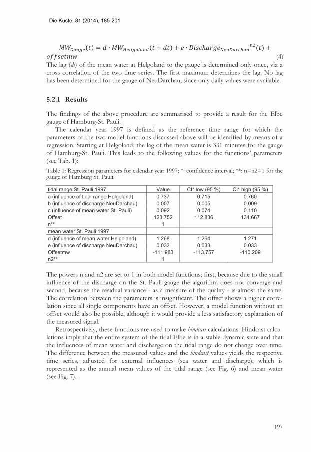
( ) = ( + ) + ( ) + (4)

The lag (dt) of the mean water at Helgoland to the gauge is determined only once, via a cross correlation of the two time series. The first maximum determines the lag. No lag has been determined for the gauge of NeuDarchau, since only daily values were available.

5.2.1 Results

The findings of the above procedure are summarised to provide a result for the Elbe gauge of Hamburg-St. Pauli.

The calendar year 1997 is defined as the reference time range for which the parameters of the two model functions discussed above will be identified by means of a regression. Starting at Helgoland, the lag of the mean water is 331 minutes for the gauge of Hamburg-St. Pauli. This leads to the following values for the functions’ parameters (see Tab. 1): Table 1: Regression parameters for calendar year 1997; *: confidence interval; **: n=n2=1 for the gauge of Hamburg St. Pauli.

tidal range St. Pauli 1997 Value CI* low (95 %) CI* high (95 %) a (influence of tidal range Helgoland) 0.737 0.715 0.760 b (influence of discharge NeuDarchau) 0.007 0.005 0.009 c (influence of mean water St. Pauli) 0.092 0.074 0.110 Offset 123.752 112.836 134.667 n** 1 mean water St. Pauli 1997 d (influence of mean water Helgoland) 1.268 1.264 1.271 e (influence of discharge NeuDarchau) 0.033 0.033 0.033 Offsetmw -111.983 -113.757 -110.209 n2** 1 The powers n and n2 are set to 1 in both model functions; first, because due to the small influence of the discharge on the St. Pauli gauge the algorithm does not converge and second, because the residual variance - as a measure of the quality - is almost the same. The correlation between the parameters is insignificant. The offset shows a higher corre-lation since all single components have an offset. However, a model function without an offset would also be possible, although it would provide a less satisfactory explanation of the measured signal.

Retrospectively, these functions are used to make hindcast calculations. Hindcast calcu-lations imply that the entire system of the tidal Elbe is in a stable dynamic state and that the influences of mean water and discharge on the tidal range do not change over time. The difference between the measured values and the hindcast values yields the respective time series, adjusted for external influences (sea water and discharge), which is represented as the annual mean values of the tidal range (see Fig. 6) and mean water (see Fig. 7).

197

Die Küste, 81 (2014), 185-201

Figure 6: Mean annual tidal range at the gauge of Hamburg-St. Pauli based on measurements and forecasts as well as their difference, which represent the signal adjusted for external influences.

Figure 7: Mean annual mean water at the gauge of Hamburg-St. Pauli based on measurements and forecasts as well as their difference, which represent the signal adjusted for external influences.

5.2.2 Evaluation of the results

Two aspects are striking when evaluating the results (Fig. 6 and Fig. 7). Since 1997 at least, the tidal range in Hamburg-St. Pauli has been clearly increasing. In the years immediately following 1997 the mean water went down by around

10 cm and then stabilised. Neither of these observations is entirely ascribable to external occurrences, but rather to inherent factors that triggered the changes. The Elbe estuary was affected by major changes during this period: not only was the fairway deepened from 13.5 to 14.4 m, sig-nificant morphological changes also took place in the Elbe delta, anthropogenic changes in the port of Hamburg and alterations in the lateral areas of the Elbe and the Nebenelbe which are in most cases associated with a decrease in volume.

198

Die Küste, 81 (2014), 185-201

NIEMEYER (2001) provides a theoretical discussion of the impacts of extension projects on the mean water. There is a close coincidence in time between the drawdown of the mean water and the fairway deepening; hence, a causal relationship is highly probable. The evolution of the tidal range presents a different picture, though, with a steady increase which is due to, firstly, the fairway deepening measures but also to the other influences mentioned before (anthropogenic and natural). This is where the regression method clearly reaches its limitations: although it indicates changes regarding a reference time range which are mainly adjusted for external influences, it is not capable of identifying the causes (anthropogenic or natural) of these changes.

Another shortcoming of the method relates to long-term trends since it implies sta-tionarity. If it is applied to a system which is subject to trends, the method learns the conditions of the reference time range but not the trend. For an evaluation it is therefore important to know the overall history and its fundamental processes and trends. In the present case, the trend of an increasing tidal range at the gauge of Hamburg-St. Pauli has already been observed over a long period of time (see WSV & HPA (2011) or FICKERT and STROTMANN (2009)). Its causes are diverse and not all of them have been identified. They are not the subject of this paper.

To conclude it should be noted that the reliability of such methods is increased if the time series used cover longer periods. Thus, after filtering the residual natural variability which is still contained in the filtered time series can be detected.

5.3 Neural networks

The core of a neural network is a regression method. The network’s topology determines the model function whose parameters are fitted (trained) using the data available. As with all regression methods there is a risk of overparameterisation if several input variables are highly correlated (multicollinearity). Since the input vector is often chosen randomly and thus cannot be reproduced, the learning algorithm used in neural networks can result in variations in the fitted parameters (weighting matrix) between trainings with the same data record. If the complexity of the model function becomes greater, the number of extrema in the solution space of an algorithm can increase. In combination with a ran-domly generated input vector for training reproducibility of the solution becomes a matter of chance.

A good understanding of the system helps to avoid using an overparameterised model along with all the deficiencies described above and to map the main processes in the network topology. To avoid multicollinearity, the correlations between the input variables have to be checked.

5.4 Other methods

Section 4.1.3 discusses the dilemma of Fourier and wavelet analyses: a very accurate fre-quency localisation requires long time series or, if a very high time resolution is used, this is only achieved at the expense of the desired high frequency resolution. There is an al-ternative, however - a relatively recent method called Hilbert Huang Transform (HHT) (see WIKIPEDIA FOR SOME EXAMPLES (2014)). This is a method that works well for signals from nonlinear and nonstationary systems. It consists of two major procedures:

199

Die Küste, 81 (2014), 185-201

the Empirical Mode Decomposition and the Hilbert Spectral Analysis. Its fundamental principle is that of instantaneous frequency (HUANG 2006). The output variables are the amplitude and frequency, both of which change over time. This method leaves behind it the familiar notion of the tide consisting of partial tides (which is in any case only a theory).

6 Conclusion

In view of the initial question this paper has discussed a small-scale example of a time series analysis of the water level in which a spectral method is combined with a simple statistical regression. The methods used must be assessed critically, in the light of their limitations, to ensure that the wrong conclusions are not drawn. In the example discussed here, the limitation is the trend: the regression method cannot account for trends because its basic assumption is stationarity.

The example does not mean that the method is restricted to the parameter water level because nearly all of the parameter time series concerning estuaries contain both a harmonic component due to the tide and a stochastic component related to meteoro-logical influences. Which methods or combinations of methods are best suited for the time series analysis depends on the signal and the specific problem.

Using benchmarks helps to ensure that an appropriate analysis method is chosen - in this case, this would mean the use of completely artificial time series whose compositions are 100 percent known. Thus the plausibility of the conclusions and the limitations of a method can be easily verified.

If there is no certainty in this respect it is also possible to use more than one method, for example an analytical method combined with a numerical simulation model. The latter is used to identify the influence factors of individual components, for example the impact of natural dynamics on the tidal range at the gauge of Hamburg-St. Pauli.

Taking this generalised approach even further, considering the methods of mathemat-ical modelling and signal analysis, it becomes obvious that, given the broadness of the topic, it is hardly possible for one single person to know about, let alone master, all these methods. Inter-institutional cooperation is therefore required in order to obtain infor-mation from the different methods and evaluate this information. Cooperation in research associations is the key to further developing the methods.

7 References

BAW: Tidewasserstandsanalysen in Ästuaren am Beispiel der Unter- und Außenelbe. Hamburg, 2007.

BAW: Hydraulic Engineering Methods. http://www.baw.de/methoden_en/index.php5/ Hydraulic_Engineering_Methods, last visited: 27.03.2014.

BERGH, J.; EKSTEDT, F. and LINDBERG, M.: Wavelets mit Anwendungen in Signal- und Bildbearbeitung. Springer-Verlag Berlin Heidelberg, Berlin, Heidelberg, Online-Ressource, 2007.

BLATTER, C.: Wavelets. Eine Einführung; [für Mathematiker, Ingenieure und Infor-matiker]. Vieweg, Braunschweig, Wiesbaden, X, 178 p., 2003.

200

Die Küste, 81 (2014), 185-201

BUTZ, T.: Fouriertransformation für Fussgänger. Teubner, Stuttgart, Leipzig, Wiesbaden, 183 p., 2003.

CARTWRIGHT, D.E.: Tides. A scientific history. Cambridge University Press, Cambridge, New York, XII, 292 p., 2000.

EUROPEAN UNION: Tide - Tidal River Development. http://www.tide-project.eu/ index.php5?node_id=Reports-and-Publications;83&lang_id=1, last visited: 27.03.2014.

FICKERT, M. and STROTMANN, T.: Zur Entwicklung der Tideverhältnisse in der Elbe und dem Einfluss steigender Meeresspiegel auf die Tidedynamik in Ästuaren. HTG-Kongress Lübeck, 2009.

GÖNNERT, G.; ISERT, K.; GIESE, H. and PLÜß, A.: Charakterisierung der Tidekurve. Die Küste, 68, 2004.

HARTUNG, J.; ELPELT, B. and KLÖSENER, K.-H.: Statistik. Lehr- und Handbuch der an-gewandten Statistik. Oldenbourg, München, Wien, XXVII, 975 S. p., 2005.

HUANG, N.E. 2006: Compact Course in The Hilbert-Huang-Transformation (HHT) For Nonlinear And Non-Stationary Time Series Analysis. Braunschweig, 2006.

KASTENS, M.: Tidewasserstandsanalyse in Ästuaren am Beispiel der Elbe. Die Küste, 72, 2007.

KASTENS, M.: Analyses of time series and model hindcast of water levels after the last deepening of the Elbe estuary - a comparison. Poster Proceedings - ICCE 2008: 31st International Conference on Coastal Engineering, 31st August to 5th Septem-ber 2008 Hamburg, Germany. Stolberg, 6-14, 2009.

LIEBIG, W.: Schließen von Lücken in Pegelaufzeichnungen. Die Küste, 56, 1994. MALCHEREK, A.: Gezeiten und Wellen. Die Hydromechanik der Küstengewässer. Vieweg

+ Teubner, Wiesbaden, IX, 301 p., 2010. MILBRADT, P.: Analyse morphodynamischer Veränderungen auf der Basis zeitvarianter

digitaler Bathymetrien. Die Küste, 78, 33-57, 2011. NIELSEN, P.: Coastal and estuarine processes. World Scientfic, Singapore, 343 p., 2009. NIEMEYER, H.D.: Change of mean tidal peaks and range due to estuarine waterway deep-

ening. Coastal Engineering Proceedings; No 26 (1998): Proceedings of 26th Con-ference on Coastal Engineering, Copenhagen, Denmark, 1998, 2001.

OPPENHEIM, A.V.; SCHAFER, R.W. and BUCK, J.R.: Zeitdiskrete Signalverarbeitung. Pear-son Studium, München, Boston [u.a.], 1031 p., 2004.

PRESS, W.H.: Numerical recipes. The art of scientific computing. Cambridge University Press, Cambridge, UK, New York, xxi, 1235 p., 2007.

PUGH, D.: Changing sea levels. Effects of tides, weather, and climate. Cambridge Univer-sity Press, Cambridge, U.K, New York, XIII, 265 p., 2004.

SIEFERT, W.: Tiden und Sturmfluten in der Elbe und ihren Nebenflüssen. Die Entwick-lung von 1950 bis 1997 und ihre Ursachen. Die Küste, 60, 1998.

SIEFERT, W. and JENSEN, J.: Fahrrinnenvertiefung und Tidewasserstände in der Elbe. Hansa, Vol. 130, 10, 1993.

WIKIPEDIA: Hilbert Huang Transform. http://en.wikipedia.org/wiki/Hilbert%E2%80% 93Huang_transform, last visited: 15.04.2014.

WSV & HPA: Abschlussbericht der Beweissicherung zur Anpassung der Fahrrinne der Unter- und Außenelbe an die Containerschifffahrt. Hamburg, 2011.

201

Die Küste, 81 (2014), 185-201