statistical discrimination, employer learning, and
TRANSCRIPT

Statistical Discrimination, Employer Learning,
and Employment Di¤erentials by Race, Gender, and Education
Seik Kim
Department of Economics
University of Washington
http://faculty.washington.edu/seikkim/
August 2012
Abstract
Previous papers on testing for statistical discrimination and employer learning require variables
that employers do not observe directly, but are observed by researchers or data on employer-
provided performance measures. This paper develops a test that does not rely on these
speci�c variables. The proposed test can be performed with individual-level cross-section data
on employment status, experience, and some variables on which discrimination is based, such
as race, gender, and education. Evidence from analysis using the March Current Population
Survey for 1977-2010 supports statistical discrimination and employer learning. The empirical
�ndings are not explained by alternative hypotheses, such as human capital theory, search and
matching models, and the theory of taste-based discrimination.
Keywords: Employer Learning, Statistical Discrimination, Unemployment Rate
JEL Classi�cation Number: J71
0I have bene�ted from helpful comments made by Joseph Altonji, Yoram Barzel, Fabian Lange, ShellyLundberg, and seminar participants at the annual meeting of the Society of Labor Economists, the meetingof the Society for the Study of Economic Inequality, the Korea Institute of Public Finance, Korea University,Sogang University, University of Washington, and the UW West Coast Poverty Center (WCPC). I gratefullyacknowledge support from the WCPC through the Emerging Poverty Scholar Small Grant.
1

1 Introduction
In hiring and wage-setting processes, employers make judgments about the value of workers
using all information available at the time of making decisions. However, the productivity
of workers is never perfectly observed, and employers must make predictions on the basis of
limited information. For example, potential workers, at the time of labor market entry, do
not have past labor market experience, and employers receive only noisy signals of worker
productivity, such as curriculum vitae, recommendation letters, and interviews, as well as
race, gender, and education. Moreover, employers�ability to screen the productivity of workers
may depend on which race, gender, or education group the workers belong to. For example,
two individuals of the same gender, education, and experience, but of di¤erent race may
face unequal opportunity in the labor market even though there is no di¤erence in their
productivity. This type of discrimination may happen because employers are less able to
evaluate the productivity of workers from one group than from another, which is also referred
to as screening discrimination by Cornell and Welch (1996).
As young workers gain more experience, past labor market performance records become
available to employers allowing them to make better predictions about their future perfor-
mance. The theory of statistical discrimination, accompanied by the employer learning hy-
pothesis, predicts that the degree of discrimination will decrease with the labor market ex-
perience of workers. Altonji and Pierret (2001) utilize this idea and propose an empirical
test for statistical discrimination. Consider variables that are correlated with productivity.
Some are directly observed by employers (e.g., education), while others are not observed by
employers, but are observed by researchers (e.g., test scores). Using the 1979 National Lon-
gitudinal Study of Youth (NLSY79), they show that if employers statistically discriminate
among young workers on the basis of easily observable characteristics, the coe¢ cients on the
easily observed variables in a wage equation should fall and the coe¢ cients on hard-to-observe
variables should rise over the worker�s period of employment.
While the recent tests of statistical discrimination require some variables available to re-
2

searchers but not observed by employers (Altonji and Pierret, 2001; Pinkston, 2006) or data
on employer-provided performance measures (Neumark, 1999; Pinkston, 2003), such variables
are di¢ cult to �nd in practice. The key contribution of this paper is proposing a test that does
not rely on those speci�c variables.1 The data requirement for the proposed strategy is mini-
mal. The theoretical model of this paper suggests that if employers statistically discriminate
among young workers on the basis of easily observable characteristics such as race, gender,
and education, but learn about their productivity over time, then the unemployment rates
for discriminated groups will be higher than those for non-discriminated groups at the time
of labor market entry and that the unemployment rates for discriminated groups will decline
faster than those for non-discriminated groups with experience. Therefore, the test can be
performed with individual-level repeated cross-section data on employment status, experience,
and some variables on which discrimination is based, such as race, gender, and education.
This paper focuses on employment opportunities rather than wage levels because discrim-
ination will in�uence the former more than the latter if the Equal Employment Opportunity
Act prohibits wage di¤erences among workers performing the same task. An obstacle to using
this approach, however, is that employment status and wage rates provide di¤erent degrees of
information: employment is measured as a binary variable, whereas wages are measured con-
tinuously. Moreover, minimal data requirements limit the scope of the analysis.2 Therefore,
to show that the predictions made by the theoretical model presented in this paper explain
the empirical results, it must be that the results cannot be explained by other hypotheses,
such as human capital theory, search and matching models, and the theory of taste-based
discrimination. This paper concludes that the empirical �ndings are not consistent with the
1A test proposed by Oettinger (1996) also does not require such variables, but requires job mobility andjob tenure information. His model suggests that the gain from job change for African-American men shouldbe smaller than that for white men. As a result, African-American men should move less and the black-whitedi¤erence in wages among men should increase with experience. Also not using those variables, Moro (2003)structurally estimates an equilibrium labor market model with statistical discrimination. His model, however,does not prove statistical discrimination as the results can also be generated by taste-based discrimination.
2Ritter and Taylor (2011) use the NLSY79 to examine whether the black-white employment gap can beexplained by the associated disparity in AFQT scores, a variable available to researchers but not observed byemployers. They �nd a large unexplained unemployment di¤erential and explain it using a model that utilizesstatistical discrimination.
3
predictions of these alternative hypotheses.
Section 2 of this paper discusses the theory of statistical discrimination and employer
learning to produce its implications on employment opportunities. Suppose that, without loss
of generality, employers classify potential workers into two groups, A and B, where signals of
group B workers are noisier than those of observationally equivalent group Aworkers. However,
employers believe that group A workers and group B workers have the same productivity
distributions. A worker�s productivity is de�ned by a �nite set of skill measures. When
employers receive applications from multiple potential workers, the employers evaluate the
applicants based on their information set and hire the subsets of applicants whose productivity
signals satisfy their own pre-set criteria. If across employers the information sets on a given
worker are fairly di¤erent and these employers require di¤erent skills, this paper shows that
more group A workers are expected to be employed than group B workers at any experience
level conditioning on observable characteristics.
As young workers gain labor market experience, the employers�beliefs about their produc-
tivity will be updated. Since relatively less information is observed for the group B workers
at the beginning of the employment process, the marginal gain of additional information is
larger for group B workers as compared to that for group A workers of the same productivity.
It also means that the distributions of employers�beliefs for the two groups will converge to
the true productivity distributions which are assumed to be the same. As a result, any gap
between group A workers and group B workers will narrow, and both groups of workers will
have more equal labor market opportunities.
Section 3 applies the proposed strategy using the March Current Population Survey (CPS)
for 1977-2010. The empirical �ndings are consistent with the theoretical predictions. First,
the results are consistent with the predictions made by employer learning. More experienced
individuals are more likely to be employed for any groups classi�ed by race, gender, and
education, and the growth rates in the employment rates are larger for the groups with initially
lower employment rates. Second, the results suggest that employers statistically discriminate
4
on the basis of race and education. Initially, black workers are less likely to be employed than
white workers when they are young, but the black-white gap in employment rates narrows with
experience conditioning on gender and education. Similarly, education is positively correlated
with the probability of becoming employed, but the employment rates of low-educated workers
grow faster than those of highly educated workers with experience conditioning on race and
gender. However, the proposed test, similar to other research, does not provide clean results
in detecting statistical discrimination on the basis of gender as females participating in the
labor force are self-selected. To verify that these empirical �ndings are not driven by a speci�c
sample, this paper also applies the test using the NLSY79 for 1979-2010 and con�rms that
the empirical �ndings are robust.
2 Theoretical Framework
2.1 Statistical Discrimination at the Time of Labor Market Entry
Consider a labor market where employers announce job vacancies and potential workers apply
for these positions. Applicants are allowed to apply for more than one position. When
employers receive applications, they screen the applicants using all information available at the
time of hiring. Each employer has his or her own pre-set productivity criteria, and applicants
may receive job o¤ers from the employer if their perceived productivity signals to the employer
meet the criteria. When there are more quali�ed applicants than open positions, employers
choose applicants based on their own hiring strategies. For example, employers may give initial
o¤ers to applicants with the highest evaluations or may choose randomly among the quali�ed
applicants. Therefore, a su¢ ciently high signal is necessary for an o¤er, but does not guarantee
an o¤er. There is no negotiation in hiring processes, but applicants with multiple job o¤ers in
hand are allowed to choose among the o¤ered jobs. When turned down, employers may give
o¤ers to other quali�ed candidates, but it can be done only for a �nite number of times due
to time constraints. As a result, some positions may remain un�lled. Other positions may not
5

be �lled due to lack of quali�ed applicants. In general, the market does not clear, and some
applicants will remain unemployed by the end of the period.
A potential worker i is characterized by the productivity, Pij, when he or she is matched
with an employer j. The productivity depends on two sets of measures, Xij and �i. Vector
Xij consists of variables that are directly observed by both employers and researchers, such as
labor market experience and possibly job tenure. We assume that race, gender, and education
are also observed by employers and researchers, but are not necessarily included in Xij. Vector
�i consists of a �nite number of skill measures, such as physical strength and IQ. Skill measures
are unobservable to researchers, but may be partly observed by some employers. We assume
that �i has a multivariate normal distribution. Since di¤erent jobs require di¤erent skills,
worker i�s productivity at job j is speci�ed through a linear combination of these factors,
Pij = r0Xij + r
0j�i; (1)
where r is a vector of parameters common to all employers and rj is an employer-speci�c non-
random weight.3 A good match occurs if a worker meets an employer who values the worker�s
skills. In other words, the quality of a match is proportional to r0j�i, the inner product of
employer j�s vector of skill weights and worker i�s vector of skill measures.
When an employer j receives applications, he or she makes predictions about the pro-
ductivity of the applicants. Let Iij denote the set of information that employer j has about
applicant i at the time when person i enter the labor market. The information set, Iij, includes
easily observable variables such as Xij as well as race, gender, and education. In principle,
however, Iij is worker-employer-speci�c and may also include factors that are not observed by
researchers and other employers. For example, if applicant i and employer j share a similar
cultural background, but applicant i0 and employer j0 do not, Iij will be richer than Ii0j or
Iij0 if other things are equal.4 A worker-employer-speci�c information set implies that di¤er-
3This setup of production is an extension of Lundberg and Startz (1983) with job-speci�c weights for avector of di¤erent abilities.
4Cultural background is broadly de�ned as in Cornell and Welch (1996) to include groups de�ned by
6

ent employers may rank the same applicant di¤erently. More speci�cally, applicant i�s true
productivity (1) is perceived by employer j as
E [PijjIij] = r0Xij + r0jE [�ijIij] : (2)
While the information sets are worker-employer-speci�c, we additionally assume that em-
ployers categorize potential workers into groups on the basis of race, gender, and/or education
and that their information sets for members of some groups are systematically richer than
those of other groups. For example, suppose that employers classify individuals into two
groups, group A and group B, but the fact that group A workers and group B workers share a
common distribution of productivity is common knowledge. Then, without loss of generality,
assume that employers have richer information sets for group A workers than for group B
workers,
Ii2A;j � Ii2B;j and Ii2A;j 6= Ii2B;j for any j: (3)
Condition (3) is equivalent to assuming that the signals from group B workers are noisier than
those from group A workers. Let Sij denote the signal that employer j receives from applicant
i�s �i. Then, a representation of (3) is assuming
Si2A;j = r0j�i + �i2A;j and Si2B;j = r
0j�i + �i2B;j; (4)
where � is a normal random variable independent of �i with E��i2A;j
�= E
��i2B;j
�= 0 and
V ar��i2A;j
�= �2A� < V ar
��i2B;j
�= �2B�. We use the common subscript i in (3) and (4) to
emphasize the fact that the two workers are identical except for their group memberships.
The information gap given in (3) has an important implication for the variances of em-
ployers� expectations in (2). It means that the ex ante variance of employer j�s perceived
productivity of group A members is strictly larger than the ex ante variance of employer j�s
language, ethnicity, school ties, neighborhood connections, or membership in social organizations, as well asrace, gender, and education.
7

perceived productivity of group B members,
V ar�E�r0j�ijIi2A;j
��> V ar
�E�r0j�ijIi2B;j
��for any j: (5)
To see this point, consider an extreme case where employer j does not have any screen-
ing ability for group B members. Then, the employer will evaluate the productivity of
any group B workers as the unconditional expectation, E [�ijIi2B;j] = E [�i], and we have
V ar�E�r0j�ijIi2B;j
��= 0. Another extreme example is the case where employer j has perfect
knowledge about the productivity of group A members, E [�ijIi2A;j] = �i. In that case, the
employer knows the productivity distribution of group A workers and V ar�E�r0j�ijIi2A;j
��will be equal to the variance of the productivity distribution, V ar
�r0j�i
�.
Another way of deriving (5) is using the information structure given in (4). That is, (2)
can be rewritten by
E [PijjIij] = E [PijjSij; Xij] = r0Xij + E�r0j�ijr0j�i + �ij
�= r0Xij +
�2��2� + �
2�
Sij; (6)
where �2� = V ar�r0j�i
�. In the �rst example above, the signal is extremely noisy, �2B� = 1,
and all applicants from group B will be evaluated as r0Xij. In the second example, the signal
is perfect, �2A� = 0, and employers observe individual productivity perfectly, r0Xij+r
0j�i. Then
we have
V ar�E�r0j�ijIi2A;j
��=
�4��2� + �
2A�
>�4�
�2� + �2B�
= V ar�E�r0j�ijIi2B;j
��for any j:
since �2A� < �2B�. Therefore, (3) implies that, conditional on Xij, group B members are
more likely to be middle-ranked, while group A members will tend to be evaluated as top- or
bottom-ranked workers. Since employers prefer more productive applicants, it is more likely
for a group A worker to receive the initial o¤er than for a group B worker.
The fact that group A members are more likely to get initial o¤ers conditional on Xij does
8

3 2 1 0 1 2 3
Group A Group B
2/33 2 1 0 1 2 3
Group A Group B
2/3
Figure 1: The Distribution of Workers�Productivity Perceived by an Employer
not necessarily imply a lower unemployment rate for group A than group B. Those who have
multiple o¤ers will decline some of their o¤ers, and the employers may move to other quali�ed
candidates. Consider an extreme case in which all employers have identical information sets.
If these employers require the same skills, they will rank all the applicants the same, and
this is equivalent to having only one employer in the entire labor market. For the market
unemployment rate to be below 50%, which is the case in most economies, workers at the left
tail of the rank distribution must be employed. Due to (5), a group A worker is more likely
to be located at the top or at the bottom than a group B worker of the same productivity,
and since the cuto¤ point for getting an o¤er is at the left tail of the distribution, the group
A unemployment rate will be higher than the group B unemployment rate.
In a more the realistic case, however, information sets are heterogeneous among employers.
Therefore, within any class of jobs that require the same skills, assume that the information
sets are random across employers. Then, workers of the same skills will be ranked di¤erently
by di¤erent employers. If there are su¢ ciently many employers, it is possible to maintain the
market unemployment rate below 50% even if each employer hires workers with signals in the
right tail of the rank distribution only. An example is presented in Figure 1. Suppose that the
expected productivity distributions for group A workers and group B workers are standard
9

normal, N (0; 1), and normal with expectation zero and standard deviation 2/3, N�0; (2=3)2
�,
respectively. Each employer has his or her pre-set productivity threshold given as a function
of his or her information set, and suppose that each employer gives o¤ers to all applicants
with signals exceeding 2/3. Then, the probability of getting an o¤er for a group A worker by
an employer is about 0.25.5 For a group B worker, the probability is about 0.16.6 If there are
ten employers in the market, since their information sets are independent of each other, the
probability of not getting an o¤er from any of the employers is 0.056 for a group A worker
and 0.175 for a group B worker.7 Therefore, the group A unemployment rate is 5.6% and the
group B unemployment rate is 17.5% in this market.
In the labor market, we expect that the unemployment rate for the group with more precise
signals (i.e., group A) will be higher when Iij is perfectly dependent across employers and that
the unemployment rate for the group with noisier signals (i.e., group B) will be higher when Iij
is random across employers. In reality, the degree of dependency will lie somewhere in-between
the two extreme cases. This paper does not provide a direct estimate of the dependency, but
we can rely on other papers to address this point. According to the statistical discrimination
literature that focuses on wage discrimination, workers in the group with noisier signals (group
B) earn lower wages than workers in the group with more precise signals (group A). In this
literature, the groups of workers with lower wages include African-Americans, women, and the
low-educated. These individuals who earn lower wages on average than individuals in other
groups, as we present later in Table 1, also have higher unemployment rates in the data. This
suggests that Iij in the real world must be more heterogeneous across employers rather than
completely identical. The discussion in this section leads to Proposition 1.
Proposition 1. When employers statistically discriminate against group B workers in
comparison to group A workers, the group B unemployment rate will be larger than the group
A unemployment rate at the time of labor market entry.
5Pr�Z > 2
3
�= 1��
�23
�= 0:25, where Z is a standard normal random variable and � (�) is its distribution
function.6Since the standard deviation is 2
3 , Pr�23Z >
23
�= 1� � (1) = 0:16.
7Note that 0:056 = (1� 0:25)10 and 0:175 = (1� 0:16)10.
10

2.2 Experience, Employer Learning, and Statistical Discrimination
Suppose that worker i accepts an o¤er from employer j. Now, worker i produces an output,
Qijt, at each experience level t = 1; 2; :::; T . Researchers, however, do not observe these
outcomes. The output, Qijt, net of the deterministic term, r0Xij, is a proxy for r0j�i of the
worker:
qijt � Qijt � r0Xij
= r0j�i + "ijt; for t = 1; 2; :::; T;
where "ijt�s are iid normal random variables withE ["i2A;jt] = E ["i2B;jt] = 0 and V ar ("i2A;jt) =
V ar ("i2B;jt) = �2" and are independent of �ij. We assume that the distributions of the "ijt�s
and rj are common knowledge and that learning on Qijt and Xij takes place publicly, so that
the entire market learns about qijt. As before, each employer has his or her own pre-set pro-
ductivity threshold for already employed workers determined by the perceived signal of the
worker�s quality and observable characteristics.
After observing qij1, qij2, ..., qijT , in each period, employer j subsequently updates his or
her initial evaluation about �i of worker i. The proof below is similar to that in Pinkston
(2006).
E [PijjIij; qij1; :::; qijT ] = r0Xij + E�r0j�ijr0j�i + �ij; r0j�i + "ij1; :::; r0j�i + "ijT
�= r0Xij +
�2�
�2� +�2"�
2�
T�2�+�2"
�2"Sij + �
2�
PTt=1 qijt
T�2� + �2"
!: (7)
As workers become more experienced, employer j learns more about their productivity, and
the distribution of evaluations approaches the true productivity distribution since
V ar (E [PijjIij; qij1; :::; qijT ]) =�4�
�2� +�2"�
2�
T�2�+�2"
11

approaches �2� as T gets larger. More importantly, the amount of learning is greater for group
B workers than group A workers. To see this, it is su¢ cient to show that the weight for the
cumulative outcomes is increasing in experience and initial noise,
d2
d�2�dT
�2�
�2� +�2"�
2�
T�2�+�2"
> 0,
but this inequality holds because
d2
d�2�dT
�2"�2�
T�2� + �2"
= �2�4"�
2��
T�2� + �2"
�3 < 0:While employed, workers are allowed to search for alternative jobs, quit their current jobs,
and move to new jobs. New o¤ers arrive with di¤erent employer-speci�c skill weights. A
worker is more likely to quit and move if the match quality of the new o¤er is better than the
quality of the current employer. In this case, workers are continuously employed and employer
learning continues. The proposed test of this paper is not a¤ected by job-to-job movements.
Learning does not take place if worker i is unemployed. There are two reasons for unem-
ployment in a period. First, worker i may have never been employed. He or she still has a
chance to �nd a job in the next period as di¤erent employers may weight his or her vector of
skills di¤erently and a new signal will be drawn from (4). Second, worker i may have been
laid o¤ by employer j and did not �nd a new job in that period. This is likely to happen
if worker i�s skill and employer j�s job-speci�c weight are not a good match or worker i was
unlucky in production. In the case of a bad match, worker i can improve the match quality
in the following period by meeting new employers, possibly those that have favorable weights
to his or her skills. In both cases, once employed, employers learn according to (7).
As workers continue to become employed from unemployment and move to new jobs from
current jobs, workers are more likely to be continuously employed, and the market learns more
precisely about the productivity of these workers. Due to (7), employers learn more about
group B workers than group A workers. Consequently, the group B unemployment rate will
12

decrease at a faster rate than the group A unemployment rate.
Proposition 2. When employers statistically discriminate against group B workers in
comparison to group A workers, and employers learn about the productivity of workers as
they accumulate more experience, the group B unemployment rate will decrease at a faster
rate than the group A unemployment rate.
3 Empirical Findings
3.1 Data
The sample is drawn from the Integrated Public Use Microdata Series (IPUMS) March Current
Population Survey (CPS) for 1977-2010. We include in the sample African-American and non-
Hispanic white men and women between the ages of 15 and 64, but exclude individuals in the
non-civilian labor force and those living in group quarters. Potential experience is obtained
by simply subtracting the number of the years of schooling and �ve from age. As a result
of this derivation, about 0.3% of the sample have negative potential experience, and these
observations are excluded from the analyses.
Table 1 reports employment rates by race, gender, education, and experience during the
sample period. Overall, employment rates increase with experience for all groups, which is
consistent with the employer learning hypothesis.8 Moreover, faster improvement in employ-
ment rates when workers are less experienced suggests that employers learn quickly as reported
in Lange (2007). Although this relationship may also be justi�ed by human capital theory or
search and matching models, these explanations will be ruled out by further analyses in later
subsections. In the data, employment rates for blacks are initially lower than whites, but the
employment rates of the former improve faster than the employment rates of the latter. This
observation is consistent with statistical discrimination on the basis of race. Table 1 reveals a
similar pattern among education groups, but not between gender groups.8This pattern is also true for a given birth cohort, but those results are not reported in this paper.
13

Table 1. Employment Rates by Race, Gender, and Education at Di¤erent Experience Levels
Potential Experience: 00-09 10-19 20-29 30-39 40-49 Total Observations
White 0.909 0.950 0.960 0.961 0.956 0.944 2,650,033
Black 0.784 0.888 0.919 0.931 0.940 0.880 365,153
Male 0.883 0.941 0.953 0.954 0.948 0.932 1,447,469
Female 0.908 0.945 0.959 0.963 0.962 0.942 1,567,717
Less than High School 0.792 0.834 0.889 0.921 0.933 0.854 585,190
High School 0.877 0.926 0.947 0.956 0.960 0.929 1,053,906
Some College 0.933 0.952 0.961 0.962 0.963 0.951 718,600
University or Above 0.968 0.978 0.979 0.976 0.973 0.976 657,490
3.2 Empirical Speci�cation and Results
This section tests for statistical discrimination and employer learning by evaluating whether
Propositions 1 and 2 hold empirically. We �rst test whether unemployment rates decline
with experience. It does not prove the existence of employer learning, but is a necessary
condition for employer learning. Human capital or search models make the same prediction.
Then, we test whether African-Americans are less likely to be employed than non-Hispanic
whites, whether females are less likely to be employed than males, and whether less educated
individuals are less likely to be employed than more educated individuals at the time of
labor market entry. It does not necessarily imply that there is statistical discrimination.
These �ndings can be supported also by human capital theory or taste-based discrimination.
Finally, we test whether the employment rates of the less-likely-to-be-employed group workers
increase at a faster rate than those of the more-likely-to-be-employed group workers. Finding
such patterns will serve as evidence of employer learning and statistical discrimination since
such patterns are not consistent with human capital theory nor taste-based discrimination.
Variables used in this analysis are employment status, race, gender, education, experience,
14

region, and birth year.9 We specify a latent variable model
Y �it = �0Gi + 0GiXit + �region + �birthyear + "it
Eit = 1 (Y �it > c) ; (8)
where Eit is an indicator for employment, Gi is a vector of easily observable variables, such as
race, gender, and education, at the time of labor market entry including an intercept, Xit is
potential experience, �region and �birthyear are region and birth year dummy variables, and "it
is an error term. The error term, "it, is treated as independent of the right hand side variables
and has a standard normal distribution. Usually, the probit estimates are not interesting by
themselves, but they are useful in this study because we are interested in their signs.
Column (1) presents an equation that includes an intercept and controls for black, expe-
rience, and black � experience. This corresponds to testing employer learning and statistical
discrimination by examining whether experience is positively associated with the probability
of employment, whether African-Americans are less likely to be employed than whites at the
time of labor market entry, and whether their group employment rate rises faster than that
of whites with experience. First, a positive experience coe¢ cient estimate, 0.125*** (0.002),
indicate the presence of employer learning. Second, a negative black coe¢ cient estimate, -
0.589*** (0.006), implies that there exists an initial black-white gap in employment rates.
Finally, a positive coe¢ cient estimate for black � experience, 0.097*** (0.003), is consistent
with the prediction in Proposition 2. In sum, the results suggest evidence of employer learning
and statistical discrimination on the basis of race.
Column (2) tests employer learning and statistical discrimination on the basis of gender.
Again, a positive experience coe¢ cient estimate, 0.134*** (0.002), implies employer learning.
However, the positive coe¢ cient for the female dummy, 0.107*** (0.005), and the negative
9The birth year dummy variables enter the model to account for di¤erences in employment rates betweencohorts of workers. For example, a 40-year-old African-American high school graduate in 1977 likely facedvery di¤erent opportunities at labor market entry than a 40-year-old worker of the same group in 2010. Thesedummy variables, however, are not the additive cohort-speci�c �xed e¤ects as the model is non-linear.
15

coe¢ cient for female � experience, -0.008*** (0.002), suggest that there is little evidence for
statistical discrimination on the basis of gender. It is tempting to conclude that men would
appear to be the discriminated group. These results, however, do not necessarily imply that
there is no statistical discrimination on the basis of gender since there are selection involved
in analyzing females�labor market participation. This point will be discussed later.
Column (3) compares high school graduate workers with university graduate workers. The
education variable is obtained by subtracting 12 from the number of the years of schooling and
then dividing it by four. In e¤ect, this variable takes on a value of zero for 12 years of schooling
(high school graduates) and one for 16 years (BA degrees or equivalent). A positive education
coe¢ cient estimate, 0.701*** (0.005), implies that education is helpful for initial employment.
The negative coe¢ cient estimate for education � experience, -0.104*** (0.002), is consistent
with employer learning and statistical discrimination on the basis of education. Overall, the
results in columns (1) and (3) are consistent with Propositions 1 and 2. African-American
workers and low-educated workers have initially worse labor market opportunities in terms of
employment probability, but their employment rates improve faster with employer learning.
Finally, column (4) includes the full set of variables. Consider eight groups of workers: all
possible combinations of race (African-American and non-Hispanic white), gender (female and
male), and education (high school graduates and university graduates). First, consider dis-
crimination on the basis of race. A negative black coe¢ cient estimate, -0.545*** (0.009), and
a positive black � experience coe¢ cient estimate, 0.093*** (0.005), suggest that high school
graduate African-American male workers are statistically discriminated against in comparison
to high school graduate white male workers. To test whether university graduate African-
American male workers are statistically discriminated against university graduate white male
workers, we examine the sum of the coe¢ cients for black and black � education, -.398***
(0.022), and the sum of the coe¢ cients for black � experience and black � education � ex-
perience, 0.041*** (0.009). The degree of racial discrimination is less for university graduates
since the magnitude of the coe¢ cients is smaller.
16

Table 2. Probit Estimates: Dependent Variable = 1 if employed, 0 if unemployed
(1) (2) (3) (4)
Constant 1.137*** 1.099*** 1.036*** 1.000***
(0.129) (0.129) (0.129) (0.129)
Black -0.589*** -0.545***
(0.006) (0.009)
Female 0.107*** 0.112***
(0.005) (0.005)
Black � Female -0.115***
(0.013)
Education 0.701*** 0.681***
(0.005) (0.007)
Black � Education 0.147***
(0.019)
Female � Education -0.040***
(0.010)
Black � Female � Education 0.156***
(0.027)
Experience/10 0.125*** 0.134*** 0.143*** 0.136***
(0.002) (0.002) (0.002) (0.002)
Black � Experience/10 0.097*** 0.093***
(0.003) (0.005)
Female � Experience/10 -0.008*** -0.007***
(0.002) (0.002)
Black � Female � Experience/10 0.047***
(0.006)
Education � Experience/10 -0.104*** -0.098***
(0.002) (0.003)
Black � Education � Experience/10 -0.053***
(0.007)
Female � Education � Experience/10 -0.002
(0.004)
Black � Female � Education � Experience/10 -0.018
(0.011)
Observations 2,245,735 2,245,735 2,245,735 2,245,735
Standard errors in parentheses. *** p<0.01, ** p<0.05, * p<0.1
17
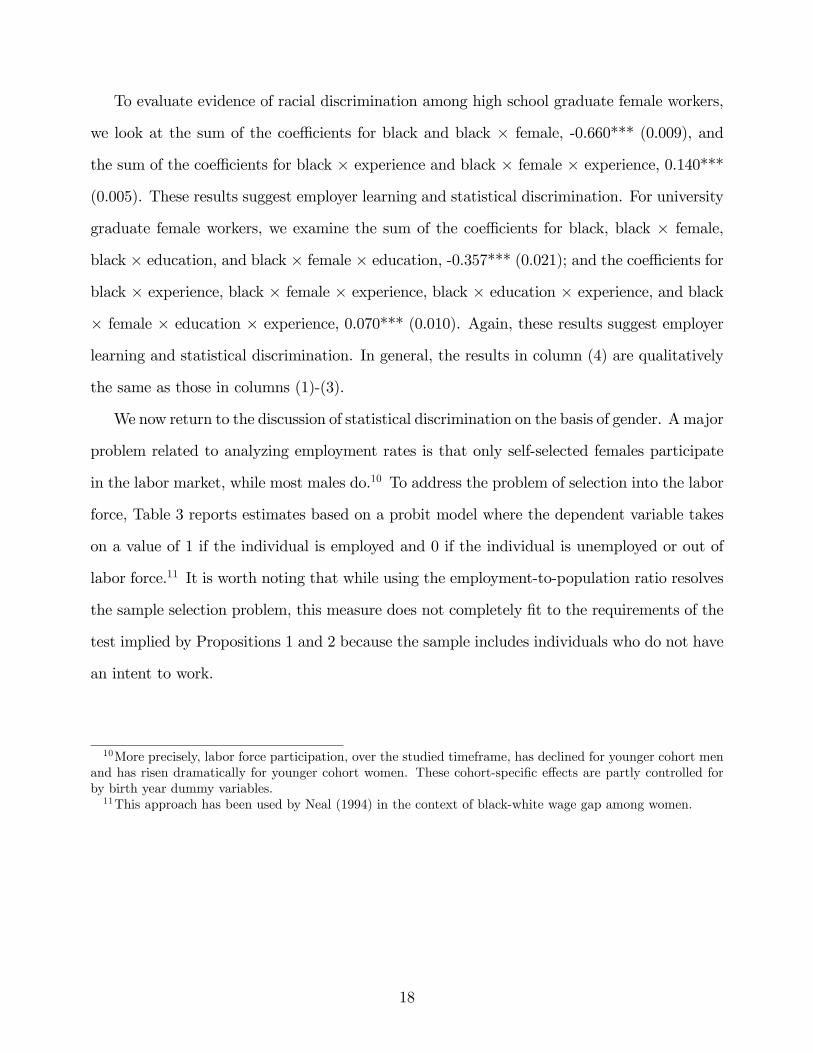
To evaluate evidence of racial discrimination among high school graduate female workers,
we look at the sum of the coe¢ cients for black and black � female, -0.660*** (0.009), and
the sum of the coe¢ cients for black � experience and black � female � experience, 0.140***
(0.005). These results suggest employer learning and statistical discrimination. For university
graduate female workers, we examine the sum of the coe¢ cients for black, black � female,
black � education, and black � female � education, -0.357*** (0.021); and the coe¢ cients for
black � experience, black � female � experience, black � education � experience, and black
� female � education � experience, 0.070*** (0.010). Again, these results suggest employer
learning and statistical discrimination. In general, the results in column (4) are qualitatively
the same as those in columns (1)-(3).
We now return to the discussion of statistical discrimination on the basis of gender. Amajor
problem related to analyzing employment rates is that only self-selected females participate
in the labor market, while most males do.10 To address the problem of selection into the labor
force, Table 3 reports estimates based on a probit model where the dependent variable takes
on a value of 1 if the individual is employed and 0 if the individual is unemployed or out of
labor force.11 It is worth noting that while using the employment-to-population ratio resolves
the sample selection problem, this measure does not completely �t to the requirements of the
test implied by Propositions 1 and 2 because the sample includes individuals who do not have
an intent to work.
10More precisely, labor force participation, over the studied timeframe, has declined for younger cohort menand has risen dramatically for younger cohort women. These cohort-speci�c e¤ects are partly controlled forby birth year dummy variables.11This approach has been used by Neal (1994) in the context of black-white wage gap among women.
18

Table 3. Probit Estimates: Dependent Variable = 1 if employed, 0 if unemployed or out of labor force
(1) (2) (3) (4)
Constant -0.371*** -0.256*** -0.465*** -0.288***
(0.049) (0.050) (0.049) (0.050)
Black -0.408*** -0.412***
(0.004) (0.006)
Female -0.216*** -0.312***
(0.003) (0.003)
Black � Female 0.137***
(0.008)
Education 0.942*** 1.081***
(0.003) (0.004)
Black � Education 0.206***
(0.012)
Female � Education -0.305***
(0.005)
Black � Female � Education 0.307***
(0.017)
Experience/10 0.045*** 0.106*** 0.057*** 0.097***
(0.001) (0.001) (0.001) (0.001)
Black � Experience/10 0.055*** 0.016***
(0.002) (0.003)
Female � Experience/10 -0.104*** -0.082***
(0.001) (0.001)
Black � Female � Experience/10 0.068***
(0.004)
Education � Experience/10 -0.169*** -0.214***
(0.001) (0.002)
Black � Education � Experience/10 -0.062***
(0.004)
Female � Education � Experience/10 0.093***
(0.002)
Black � Female � Education � Experience/10 -0.042***
(0.006)
Observations 3,015,186 3,015,186 3,015,186 3,015,186
Standard errors in parentheses. *** p<0.01, ** p<0.05, * p<0.1
19

The results for gender in Table 3 are quite di¤erent from those in Table 2. In column
(2) of Table 3, initially females work less, -0.216*** (0.003), and the proportion of working
females does not change much over experience since the sum of the coe¢ cients for experience
and female � experience is close to zero, 0.002* (0.001). In column (4), white high school
graduate females works less than observationally equivalent males initially, -0.312*** (0.003),
and the proportion of working white high school graduate females decreases with experience:
the sum of the coe¢ cients for experience and female � experience is 0.015*** (0.001). Similar
patterns are found for females of other race and education groups. In sum, these results
suggest that statistical discrimination on the basis of gender cannot be tested by Propositions
1 and 2 since they do not consider sample selection.
3.3 Evidence from the NLSY79
In this subsection, we apply the proposed test to a sample drawn from the NLSY79 for 1979-
2010. This exercise is useful in several aspects. First of all, we can verify whether the empirical
�ndings are robust to other data sets and compare our �ndings with those of previous papers
on wage discrimination. Second, the NLSY79 individuals are born over a narrow period of
1957-1964, and this alleviates concerns about cohort e¤ects.
From the NLSY79, we include in our sample the cross-sectional sample of whites and blacks
and the oversample of blacks. In this approach, an individual in a given year is classi�ed
as unemployed if he or she was in the labor force for at least 26 weeks of the year and was
unemployed for at least half of the period while in the labor force. This measure is constructed
using three variables: the numbers of weeks employed, unemployed, and out of labor force.
Observations with any of the three variables missing are dropped. In addition, among the
non-missing observations, for about 3% of the sample the three variables do not add up to 52
and are excluded from the analyses. The overall unemployment rate of the sample is 6.36%,
and the unemployment rate estimate is quite stable under di¤erent classi�cations.
20

Table 4. Probit Estimates from the NLSY79: Dependent Variable = 1 if employed, 0 if unemployed
(1) (2) (3) (4)
Constant 1.804*** 1.549*** 1.301*** 1.487***
(0.105) (0.103) (0.111) (0.113)
Black -0.730*** -0.601***
(0.022) (0.031)
Female 0.080*** 0.119***
(0.021) (0.032)
Black � Female -0.295***
(0.046)
Education 0.733*** 0.607***
(0.023) (0.042)
Black � Education 0.059
(0.064)
Female � Education 0.018
(0.066)
Black � Female � Education 0.378***
(0.099)
Experience/10 0.106*** 0.132*** 0.160*** 0.171***
(0.010) (0.010) (0.007) (0.015)
Black � Experience/10 0.077*** 0.008
(0.014) (0.020)
Female � Experience/10 -0.011 -0.075***
(0.014) (0.021)
Black � Female � Experience/10 0.167***
(0.030)
Education � Experience/10 -0.111*** -0.044
(0.015) (0.028)
Black � Education � Experience/10 -0.034
(0.042)
Female � Education � Experience/10 -0.045
(0.042)
Black � Female � Education � Experience/10 -0.118*
(0.062)
Observations 119,980 119,980 119,980 119,980
Standard errors in parentheses. *** p<0.01, ** p<0.05, * p<0.1
21

Table 4 presents the probit estimates, where the dependent variable is one minus the
unemployment rate. Overall, the NLSY79 estimates are qualitatively the same as the CPS
estimates in Table 2.12 In column (1), employer learning and statistical discrimination on the
basis of race are supported by a negative black coe¢ cient estimate, -0.730*** (0.022) and a
positive coe¢ cient estimate for black � experience, 0.077*** (0.014). In column (4), where
the full set of variables are included, the corresponding estimates are -0.601*** (0.031) and
0.008 (0.020). The evidence of learning is weaker, but the estimates have the expected signs.
Column (2) presents employer learning and statistical discrimination on the basis of gender,
and similar to the CPS results the evidence is not very clear. In column (3), the positive
coe¢ cient estimate for education, 0.607*** (0.042), and the negative coe¢ cient estimate for
education� experience, -0.111*** (0.015), are consistent with employer learning and statistical
discrimination on the basis of education. This evidence is weaker in column (4), but the signs
of the estimates are consistent with Propositions 1 and 2.
3.4 Discussion and Alternative Explanations
This subsection discusses whether or not the predictions made by the theoretical model pre-
sented in this paper can also be explained by other hypotheses, such as human capital theory,
search and matching models, and the theory of taste-based discrimination as alternative hy-
potheses. We �nd that these alternative explanations, at least as currently developed, are not
adequate in explaining the estimates of this paper.
With regard to human capital theory, so far in the discussion, the rate of human capital
attainment is set to be the same for the two groups of workers. However, a more realistic
assumption is that group B workers have fewer opportunities for human capital investment
than to group A workers.13 Employers may give fewer training or promotion opportunities to
12A table that corresponds to Table 3 for the NLSY79 is not reported in this paper, but the results are againvery similar to those in Table 3. In this case, not working is de�ned by being unemployed or out of labor forcefor at least 26 weeks of the year.13It is possible that disadvantaged workers get more on-the-job training once hired. Holzer and Neumark
(2000) �nd that African-American male workers spend more time with supervisors or coworkers in the presenceof a¢ rmative action. However, there is no clear evidence that this informal training leads to a higher rate of
22

group B workers than group A workers. Moreover, if African-Americans get more education
than whites of similar cognitive ability, as Lang and Manove (2011) �nd, African-Americans
would have fewer chances for training conditional on education. Then, the parameter vector
r in (1) will be di¤erent for each of the two groups, and it will be more di¢ cult for the
prediction in Proposition 2 to hold even if there is statistical discrimination in opportunities
for human capital investment. However, this also implies that �nding the pattern predicted
by Proposition 2 in the data will serve as strong evidence of statistical discrimination and
employer learning. Therefore, the results in Table 2 support the hypotheses.
Next, we consider the theory of taste-based discrimination. In a static model, this theory
can explain why discriminated groups have lower employment rates at any experience level,
but it cannot explain why the gaps in employment rates between discriminated and non-
discriminated groups narrow with experience. In our results, there is the possibility for taste-
based discrimination since the two employment rates do not fully converge at experience level
40-49. However, even if the entire employment gap at the highest experience level is due to
taste-based discrimination, it explains less than a two percentage point di¤erence between
discriminated and non-discriminated groups.
Finally, we discuss whether taste-based discrimination accompanied by search models can
produce results that are consistent with the empirical results of this paper. This discussion
relies heavily on Lang and Lehmann (2011). We begin by presenting Table 5, where the men�s
black-white employment gap is much larger among low-educated than among high-educated
workers.14 Lang and Lehmann state that this pattern is not explained by any search model,
even though there has been an increase in research in this �eld of search models with taste-
based discrimination. Moreover, they point out that while taste-based discrimination models
can generate wage and unemployment duration di¤erentials between group A workers and
group B workers when combined with search, no existing model for taste-based discrimination
can explain the unemployment di¤erential.
human capital investment. They �nd, however, that women get sign�cantly more formal on-the-job trainingwhen a¢ rmative action is present.14Further conditioning on birth year does not change the pattern qualitatively.
23

Table 5. Male�s Employment Rates by Race and Education
at Di¤erent Experience Levels
Potential Experience: 00-09 10-19 20-29 30-39 40-49 Total
White
Less than High School 0.801 0.850 0.896 0.923 0.929 0.862
High School 0.883 0.929 0.948 0.953 0.955 0.930
Some College 0.933 0.955 0.962 0.961 0.959 0.952
University or Above 0.967 0.981 0.979 0.976 0.972 0.977
Black
Less than High School 0.581 0.769 0.851 0.894 0.908 0.776
High School 0.764 0.872 0.897 0.915 0.947 0.862
Some College 0.855 0.911 0.929 0.929 0.941 0.905
University or Above 0.933 0.952 0.965 0.954 0.970 0.952
4 Concluding Remarks
This paper proposes a new testing procedure for statistical discrimination and employer learn-
ing using basic individual characteristic variables. The test can be performed with individual-
level cross-section data on employment status, experience, and some variables on which dis-
crimination is based, such as race, gender, and education. The theoretical model produces
testable implications for employment rates in the presence of statistical discrimination and
employer learning. When employers statistically discriminate against some workers in com-
parison to other workers, the discriminated group�s unemployment rate will be larger than
the non-discriminated group�s unemployment rate at the time of labor market entry. The
theory of statistical discrimination, accompanied by the employer learning hypothesis, pre-
dicts that the discriminated group�s unemployment rate will decrease at a faster rate than the
non-discriminated group�s unemployment rate as workers become more experienced.
Empirical �ndings based on the CPS support employer learning and statistical discrimi-
nation on the basis of race and education. Replicating the test using the NLSY79, the data
24

set which others have extensively used in this literature, supports the validity of the proposed
test. This paper provides a theory for one of the well-known empirical regularities that the
black-white employment gap is larger among low-skilled than among high-skilled workers. Al-
ternative hypotheses do not produce results that are consistent with the empirical �ndings of
this paper, but this does not imply that the proposed test completely rules out the possibility
of alternative explanations. It would be useful to explore other approaches to �nd evidence
for discrimination and learning, and these are left for future research.
5 References
Altonji, Joseph G. 2005. �Employer Learning, Statistical Discrimination and Occupational
Attainment.�American Economic Review (Papers and Proceedings), 95(2), 112-117.
Altonji, Joseph G., and Charles R. Pierret. 2001. �Employer Learning and Statistical Dis-
crimination.�Quarterly Journal of Economics, 116 (1, February), 313-350.
Cornell, Bradford and Ivo Welch. 1996. �Culture, Information, and Screening Discrimina-
tion.�Journal of Political Economy, 104(3, June), 542�571.
Holzer, Harry J. and David Neumark. 2000. �What Does A¢ rmative Action Do?�Industrial
and Labor Relations Review, 53(2, Jan), 240-271.
Lang, Kevin and Michael Manove. 2011. �Education and Labor Market Discrimination.�
American Economic Review, 101(3, June). 1467�1496.
Lang, Kevin and Jee-Yeon K. Lehmann. 2011. �Racial Discrimination in the Labor Market:
Theory and Empirics.�NBERWorking Paper, forthcoming in Journal of Economic Literature.
Lange, Fabian. 2007. �The Speed of Employer Learning.�Journal of Labor Economics, 25(1),
651-691.
Lundberg, Shelly J. and Richard Startz. 1983. �Private Discrimination and Social Intervention
in Competitive Labor Markets,�American Economic Review, 73(3, June), 340-347.
Moro, Andrea. 2003. �The E¤ect of Statistical Discrimination on Black�White Wage Inequal-
25

ity: Estimating a Model with Multiple Equilibria,� International Economic Review, 44(2),
467-500.
Neal, Derek. 2004. �The Measured Black-White Wage Gap among Women Is Too Small.�
Journal of Political Economy, 112(1): S1�28.
Neumark, David. 1999. �Wage Di¤erentials by Race and Sex: the Roles of Taste Discrimina-
tion and Labor Market Information.�Industrial Relations, 38(3), 414-442.
Oettinger, Gerald S. 1996. �Statistical Discrimination and the Early Career Evolution of the
Black-White Wage Gap.�Journal of Labor Economics, 14(1, Jan.), 52-78.
Pinkston, Joshua C. 2003. �Screening Discrimination and the Determinants of Wages.�Labour
Economics, 10(6, November), 643-658.
Pinkston, Joshua C. 2006. �A Test of Screening Discrimination with Employer Learning.�
Industrial and Labor Relations Review, 59(2, January), 267-284.
Ritter, Joseph A. and Lowell J. Taylor. 2011. �Racial Disparity in Unemployment.�Review
of Economics and Statistics, 93(1), 30-42.
26