statistical computing for scientists and engineers computing for scientists and engineers prof....

Statistical Computing, University of Notre Dame, Notre Dame, IN, USA (Fall 2018, N. Zabaras)

Statistical Computing for Scientists and Engineers

Prof. Nicholas Zabaras

Center for Informatics and Computational Science

https://cics.nd.edu/

University of Notre Dame

Notre Dame, Indiana, USA

Email: [email protected]

URL: https://www.zabaras.com/

August 21, 2018

1


mailto:[email protected]

http://mpdc.mae.cornell.edu/


Two lectures each week TThu 12:30-1:45

Recitation (not mandatory) F 11:30-12:20.

Teaching Assistants: Nicholas Geneva, Govinda Anantha-

Padmanabha, Navid Shervani-Tabar

Office Hours: (NZ, Cushing 311I) M 1-2 pm, F 1-2 pm; (TAs) M 5-7 pm

Occasionally lectures on Friday.

All information regarding the course will be posted on the webpage.

This includes video lectures, slides, references, homework, etc.

Grades based on Homeworks (60%), Final Project (40%)

Course Organization

2

https://www.zabaras.com/statisticalcomputing

https://www.zabaras.com/statisticalcomputing


C Bishop, Pattern Recognition and Machine Learning

K Murphy, Machine Learning: A Probabilistic Perspective

JS Liu, Monte Carlo Strategies in Scientific Computing.

CP Robert, Monte Carlo Statistical Methods.

A Gelman, JB Carlin, HS Stern and DB Rubin, Bayesian Data Analysis.

CP Robert, The Bayesian Choice: from Decision-Theoretic Motivations

to Computational Implementation.

ET Jaynes, Probability Theory: The Logic of Science.

Additional references to journal publications will be provided (with html links) in

each lecture.

Books

3

http://research.microsoft.com/en-us/um/people/cmbishop/PRML/index.htm

https://www.amazon.com/dp/0262018020

https://www.amazon.com/Strategies-Scientific-Computing-Springer-Statistics/dp/0387763694

https://www.ceremade.dauphine.fr/~xian/books.html

https://www.amazon.com/Bayesian-Analysis-Edition-Chapman-Statistical/dp/158488388X/ref=sr_1_1?ie=UTF8&qid=1358259596&sr=8-1&keywords=Gelman,+JB+Carlin,+HS+Stern+and+DB+Rubin,+Bayesian+Data+Analysis

https://www.ceremade.dauphine.fr/~xian/books.html#BA

https://www.amazon.com/Probability-Theory-Science-T-Jaynes/dp/0521592712


Course Objectives

4

To introduce statistical methods used for the stochastic simulation of

complex physical systems in the context of Bayesian analysis.

Introduce Monte Carlo and approximate inference techniques in the

context of Bayesian models, and parametric and non-parametric

models for supervised and unsupervised learning.

Acquaint students with a set of powerful tools and theories that can be

directly transitioned to their research independently of their field.

The course is appropriate for graduate students in Engineering,

Chemical/Physical and Biological Sciences, Mathematics/Statistics/

Computer Science.


Motivation

5

Why Monte Carlo and Approximate Inference

To deal with uncertainties that are omnipresent in physical systems

To perform computational tasks (e.g. integration) in high

dimensional spaces.

Why Bayesian?

To draw inferences from data. This data is collected experimentally

or produced computationally.

To quantify uncertainties associated with these inferences.

To quantify predictive uncertainties.


Bayesian Statistics

6

Why is it relevant to Science & Engr? It is highly suitable to many problems from diverse areas:

From physics and chemistry to genetics, from econometrics

to machine learning.

Allows principled incorporation of prior knowledge/

information/beliefs.

This is a vice and a virtue.

Readily handle missing or corrupted data, outliers.

Why now? Bayesian Statistics have enjoyed a surge of popularity in

the last 25 years.

This has coincided with advances in Scientific Computation.

Bayesian models, powerful as they may be, are analytically

intractable.

Most often one must resort to Approximate Inference or

Monte Carlo.


Topics to Cover

7

1. Basics of Probability, Statistics, and Information Theory.

2. Foundamentals of Bayesian Statistics: Prior, Likelihood,

Posterior, Predictive Distributions3. Bayesian Inference: Applications to Regresssion, Classification,

Model Reduction, etc.

4. Monte Carlo Methods: Applications to Dynamical Systems,

Time Series Models, HMM, Probabilistic Robotics, etc.

5. State Space Models

6. Sparse Bayesian Models

7. Bayesian Model Selection

8. Expectation-Maximization, Mixture Models

9. Variational Methods, Approximate Inference (an introduction)

10. Other (if time allows)


Introduction to Probability and Statistics

Prof. Nicholas Zabaras

Center for Informatics and Computational Science


University of Notre Dame

Notre Dame, Indiana, USA

Email: [email protected]

URL: https://www.zabaras.com/

August 21, 2018

8


mailto:[email protected]

http://mpdc.mae.cornell.edu/


Fundamentals of Probability Theory

Discrete random variables

Bayes rule

Independence and conditional independence

Contents

9


References

10

• Following closely Chris Bishops’ PRML book, Chapter 2.

• Kevin Murphy’s, Machine Learning: A probablistic perspective, Chapter 2.

• Jaynes, E. T. (2003). Probability Theory: The Logic of Science. Cambridge

University Press.

• Bertsekas, D. and J. Tsitsiklis (2008). Introduction to Probability. Athena

Scientific. 2nd Edition.

• Wasserman, L. (2004). All of statistics. A Concise Course in Statistical

Inference. Springer.

http://research.microsoft.com/en-us/um/people/cmbishop/PRML/index.htm

http://www.cs.ubc.ca/~murphyk/MLbook/

http://omega.albany.edu:8008/JaynesBook.html

https://www.google.com/url?sa=t&rct=j&q=&esrc=s&source=web&cd=2&cad=rja&uact=8&ved=0ahUKEwjGi8qBsavUAhUJWxQKHe6JA8EQFggwMAE&url=http://sanghv.com/download/soft/Machine Learning, Artificial Intelligence, Mathematics eBooks/math/probability/introduction to probability (bertsekas, 2nd, 2008).pdf&usg=AFQjCNFcVnETxkkD10T7-FQgAxFT_nu9pw&sig2=vt6iFJFO89_zA7jowynazg

https://link.springer.com/book/10.1007/978-0-387-21736-9


Frequentisit Probability: Long run frequencies of `events’

Bayesian Probability: Quantifying our uncertainty about something

It can be used to model our uncertainty about events that do not

have long term frequencies

E.g. the event that the polar ice cap will melt by 2020

The rules of probability are the same for both approaches.

For more details: S. Ross, Introduction to Probability Models

Frequentist Vs Bayesian

11

http://www.amazon.com/Introduction-Probability-Models-Tenth-Edition/dp/0123756863/ref=dp_ob_title_bk


Sample space: Set of all possible outcomes of an experiment.

Ω = {1, 2, 3, 4, 5, 6} is the sample space for the numbers that appear on

a die rolled once.

For more details: S. Ross, Introduction to Probability Models

Event: A subset of the sample space.

If 𝐸 = {5} then 𝐸 is the event of rolling a 5.

If 𝐸 = {𝐽, 𝑄, 𝐾} the 𝐸 is the event of getting a face card.

Sample Space

12

http://www.amazon.com/Introduction-Probability-Models-Tenth-Edition/dp/0123756863/ref=dp_ob_title_bk


union operator: For any two events 𝐸 and 𝐹 of a sample space Ω,we define the new event to consist of all outcomes that are either in

𝐸 or in 𝐹 or in both 𝐸 and 𝐹.

If 𝐸 = {1, 5} and 𝐹 = {3} then = {1, 3, 5} is the event of rolling

an odd number.

E F

intersection operator: For any two events 𝐸 and 𝐹 of a sample

space Ω, we define the new event to consist of all outcomes that

are in both 𝐸 and 𝐹.

If 𝐸 = {1, 3, 5} and 𝐹 = {3} then 𝐸 ∩ 𝐹 = {3} is the event of rolling a

three.

If 𝐸 = {𝐽, 𝑄, 𝐾} and 𝐹 = {10, 𝐾} then 𝐸 ∩ 𝐹 = {𝐾} is the event of

getting a King.

If 𝐸 = {𝐻} and 𝐹 = {𝑇} then would not consist of any

outcomes and would thus not occur. If , then 𝐸 and 𝐹 are said

to be mutually exclusive ( is called the empty set).

Union and Intersection

13

E F

E F

E F

E F


Likewise, describes the union of events 𝐸1, 𝐸2, . . . and corresponds to

outcomes that are in 𝐸𝑖 for at least one value of 𝑖 = 1, 2, . . . .

describes the intersection of events 𝐸1, 𝐸2, . . . and corresponds to

outcomes that are in all events 𝐸𝑖 , 𝑖 = 1, 2, . . . .

More than two Events

14


Pr(𝐸): The probability of event 𝐸. It is a number satisfying the following

three conditions:

1) 0 ≤ Pr(𝐸) ≤ 1.

2) Pr(Ω) = 1, and

3) For any sequence of events 𝐸1, 𝐸2, . . . that are mutually exclusive (i.e.,

) when i≠j, the following holds:i jE E

Pr( ) 0.

11

Pri i

ii

P E E

Laws of Probability

15


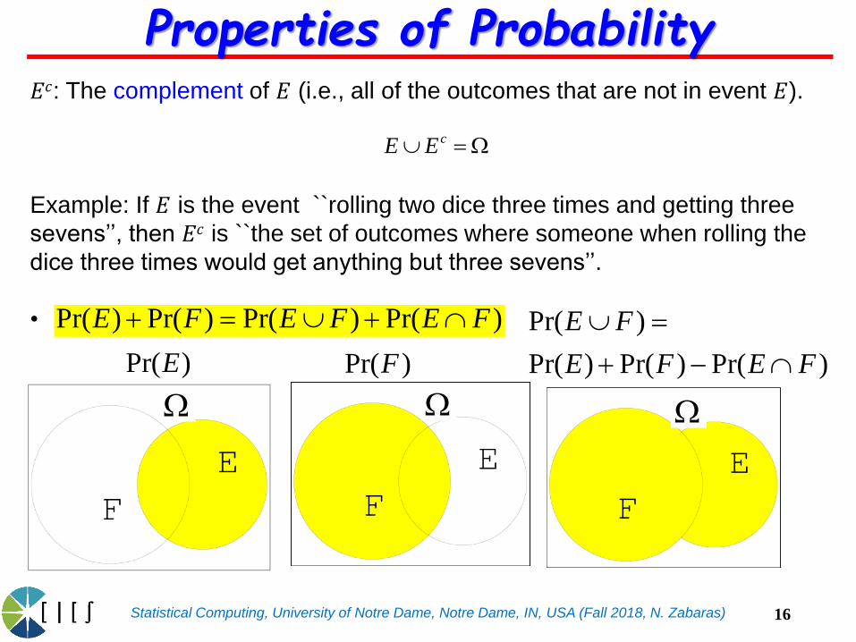
𝐸𝑐: The complement of 𝐸 (i.e., all of the outcomes that are not in event 𝐸).

Example: If 𝐸 is the event ``rolling two dice three times and getting three

sevens’’, then 𝐸𝑐 is ``the set of outcomes where someone when rolling the

dice three times would get anything but three sevens’’.

•

cE E

Properties of Probability

16

Pr( ) Pr( ) Pr( ) Pr( )E F E F E F

Pr( )E Pr( )F

Pr( )

Pr( ) Pr( ) Pr( )

E F

E F E F


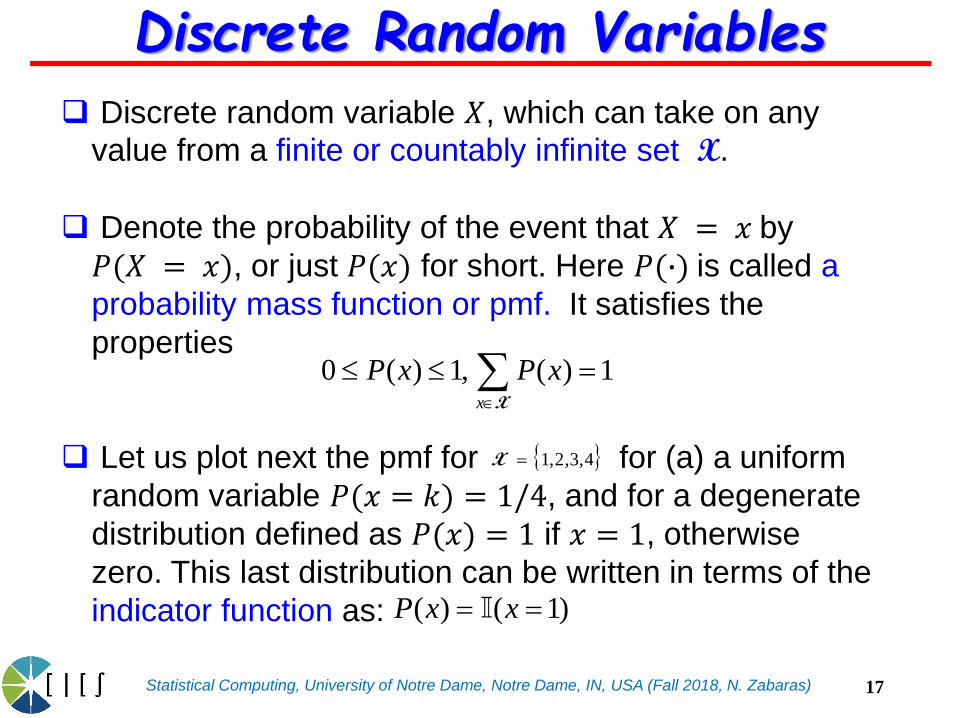
Discrete random variable 𝑋, which can take on any

value from a finite or countably infinite set X.

Denote the probability of the event that 𝑋 = 𝑥 by

𝑃(𝑋 = 𝑥), or just 𝑃(𝑥) for short. Here 𝑃(∙) is called a

probability mass function or pmf. It satisfies the

properties

Let us plot next the pmf for for (a) a uniform

random variable 𝑃(𝑥 = 𝑘) = 1/4, and for a degenerate

distribution defined as 𝑃(𝑥) = 1 if 𝑥 = 1, otherwise

zero. This last distribution can be written in terms of the

indicator function as:

Discrete Random Variables

17

0 ( ) 1, ( ) 1x

P x P x

X

1,2,3,4X

( ) ( 1)P x x


Discrete Random Variables: Example

18

( ) 1/ 4P x

1,2,3,4X

( ) ( 1)P x x

0 1 2 3 4 50

0.25

0.5

0.75

1

0 1 2 3 4 50

0.25

0.5

0.75

1

1,2,3,4X

Run MatLab function discreteProbDistFig from Kevin Murphys’ PMTK

https://github.com/probml/pmtk3/blob/master/demos/discreteProbDistFig.m

https://github.com/probml/pmtk3


Probability theory provides a consistent framework for

the quantification and manipulation of uncertainty.

It forms one of the central foundations for pattern

recognition and machine learning.

The probability that 𝑋 will take the value 𝑥𝑖 and 𝑌 will

take the value 𝑦𝑗 is written 𝑃(𝑋 = 𝑥𝑖 , 𝑌 = 𝑦𝑗) and is

called the joint probability of 𝑋 = 𝑥𝑖 and

𝑌 = 𝑦𝑗 .

Here is the number of times (in 𝑁 trials) that the

event occurs. Similarly is the number

of times that occurs.

( , )ij

i j

nP X x Y y

N

Joint Probability

19

ijn

,i jX x Y y ic

iX x


Even complex calculations in probability are simply

derived from the sum and product rules of probability.

Sum Rule:

Product Rule:

The product rule leads to the Chain Rule:

1

( ) ( , )L

i i j

j

P X x P X x Y y

( , )

( | ) ( )

ij ij ii j

i

j i i

n n cP X x Y y

N c N

P Y y X x P X x

The Sum and Product Rules

20

1: 1 2 1 3 1 2 1: 1( ) ( ) ( | ) ( | , )... ( | )D D DP X P X P X X P X X X P X X


Even complex calculations in probability are simply

derived from the sum and product rules of probability.

Sum Rule:

Product Rule:

( ) ( , )P x P x y dy

( , ) ( | ) ( ) ( | ) ( )P x y P x y P y P y x P x

The Sum and Product Rules

21


Bayes’ theorem plays a central role in pattern

recognition and machine learning

The normalizing factor 𝑃(𝑌) is given as:

'

( , ) ( ) ( | )( | )

( ) ( ') ( | ')x

P X x Y y P X x P Y y X xP X x Y y

P Y y P X x P Y y X x

'

( ) ( , ) ( ') ( | ')X x

P Y y P X Y y P X x P Y y X x

Conditional Probability and Bayes’ Rule

22


Suppose a red and a blue

box with probabilities of selecting

each of them being

𝑃 𝐵 = 𝑟 =4

10<

1

2,

𝑃(𝐵 = 𝑏) = 6/10.

We select an orange. What is

the probability that we chose

from the red box ?

Then:

( ) ( | ) ( ) ( | ) ( )

6 4 1 6 9

8 10 4 10 20

P F o P F o B r P B r P F o B b P B b

6 4

( | ) ( ) 2 18 10( | )9( ) 3 2

20

P F o B r P B rP B r F o

P F o

O

A

O O

O OO

A

O

A A A

Example of Bayes’ Theorem

23

( | )P B r F o


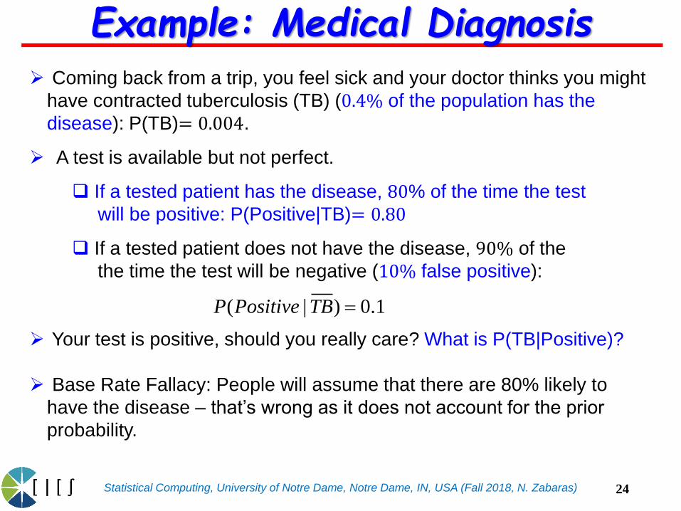
Example: Medical Diagnosis

24

Coming back from a trip, you feel sick and your doctor thinks you might

have contracted tuberculosis (TB) (0.4% of the population has the

disease): P(TB)= 0.004.

A test is available but not perfect.

If a tested patient has the disease, 80% of the time the test

will be positive: P(Positive|TB)= 0.80

If a tested patient does not have the disease, 90% of the

the time the test will be negative (10% false positive):

Your test is positive, should you really care? What is P(TB|Positive)?

Base Rate Fallacy: People will assume that there are 80% likely to

have the disease – that’s wrong as it does not account for the prior

probability.

( | ) 0.1P Positive TB


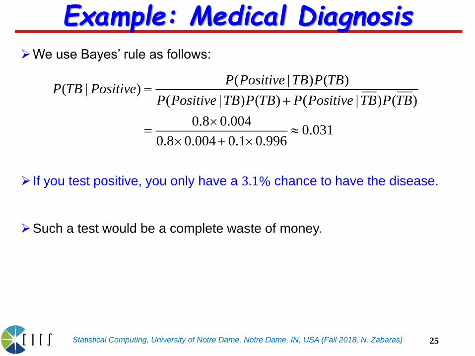
Example: Medical Diagnosis

25

We use Bayes’ rule as follows:

If you test positive, you only have a 3.1% chance to have the disease.

Such a test would be a complete waste of money.

( | ) ( )( | )

( | ) ( ) ( | ) ( )

0.8 0.0040.031

0.8 0.004 0.1 0.996

P Positive TB P TBP TB Positive

P Positive TB P TB P Positive TB P TB


Here we classify feature vectors 𝒙 to classes using the

above posterior.

It is a generative classifier as it specifies how to

generate data 𝒙 using the class-conditional probabilities

and class priors .

In a discriminative setting, the posterior is

directly fitted.

'

( | ) ( | , )( | , )

( ' | ) ( | ', )x

P y c P y cP y c

P y c P y c

x

xx

Example: Generative Classifier

26

( | )P y c ( | , )P y c x

( | )P y c x


Two events 𝐴 and 𝐵 are independent (written as ) if

Conditional probability: Probability that 𝐴 happens

provided that 𝐵 happens,

Using the above Eqs, we see that for independent events,

( )

( | ) : ( | ) ( )( )

P A BP A B Note P A B P A B

P B

( ) ( ) ( )P A B P A P B

( | ) ( )P A B P A

27

Independency, Conditional Probability

A B


𝑋 and 𝑌 are unconditionally independent or marginally

independent, denoted , if we can represent the joint

as the product of the two marginals

𝑋 and 𝑌 are conditionally independent (CI) given 𝑍 iff the

conditional joint can be written as a product of conditional

marginals:

28

Independence, Conditional Independence

X Y

( , ) ( ) ( )X Y P X Y P X P Y

| ( , | ) ( | ) ( | )X Y Z P X Y Z P X Z P Y Z


Pairwise independence does not imply mutual

independence.

Consider 4 balls (numbered 1,2,3,4) in a box. You draw

one at random. Define the following events:

Note that the three events are pairwise independent,

e.g.

However:

29

Pairwise Vs. Mutual Independence

1

2

3

: 1 2

: 2 3

: 1 3

X ball or is drawn

X ball or is drawn

X ball or is drawn

1 2 1 2 1 2

1/2 1/2

1( , ) ( ) ( )

4X X P X X P X P X

1 2 3 1 2 3

1/2 1/2 1/2

1( , , ) 0, ( ) ( ) ( )

8P X X X P X P X P X


Consider the following example. Define:

Event 𝑎 = `it will rain tomorrow’

Event 𝑏 =`the ground is wet today’ and

Event 𝑐 =`raining today’.

𝑐 causes both 𝑎 and 𝑏 – thus given 𝑐 we don’t need to

know about 𝑏 to predict 𝑎

Observing a “root node”, separates “the children”!

30


| ( , | ) ( | ) ( | )a b c P a b c P a c P b c

| ( | , ) ( | )a b c P a b c P a c


Assume unconditional independence . Let 𝑋 take 6values and 𝑌 takes 5 values. The cost for defining 𝑝(𝑋, 𝑌)is drastically reduced if .

The parameters are reduced from 29 (= 30 − 1) to 9 =5 + 4 = (6 − 1) + (5 − 1).a Independence is key to

efficient probabilistic modeling (naïve Bayes classifiers,

Markov Models, graphical models, etc.). a We subtract one on the counts to account for the sum-to-one probability constraint rule.

31


X Y

X Y

statistical computing for scientists and engineers computing for scientists and engineers prof....

Documents