statistical applications in genetics and molecular biology · provides a uniﬁed statistical model...

Statistical Applications in Geneticsand Molecular Biology

Volume 8, Issue 1 2009 Article 47

A Unified Mixed Effects Model for Gene SetAnalysis of Time Course Microarray

Experiments

Lily Wang∗ Xi Chen† Russell D. Wolfinger‡

Jeffrey L. Franklin∗∗ Robert J. Coffey†† Bing Zhang‡‡

∗Vanderbilt University, [email protected]†Vanderbilt University, [email protected]‡SAS Institute Inc., [email protected]

∗∗Vanderbilt University, [email protected]††Vanderbilt University, [email protected]‡‡Vanderbilt University, [email protected]

Copyright c©2009 The Berkeley Electronic Press. All rights reserved.

A Unified Mixed Effects Model for Gene SetAnalysis of Time Course Microarray

Experiments∗

Lily Wang, Xi Chen, Russell D. Wolfinger, Jeffrey L. Franklin, Robert J. Coffey,and Bing Zhang

Abstract

Methods for gene set analysis test for coordinated changes of a group of genes involved inthe same biological process or molecular pathway. Higher statistical power is gained for gene setanalysis by combining weak signals from a number of individual genes in each group. Althoughmany gene set analysis methods have been proposed for microarray experiments with two groups,few can be applied to time course experiments. We propose a unified statistical model for analyz-ing time course experiments at the gene set level using random coefficient models, which fall intothe more general class of mixed effects models. These models include a systematic componentthat models the mean trajectory for the group of genes, and a random component (the randomcoefficients) that models how each gene’s trajectory varies about the mean trajectory.

We show that the proposed model (1) outperforms currently available methods at discriminatinggene sets differentially changed over time from null gene sets; (2) provides more stable results thatare less affected by sampling variations; (3) models dependency among genes adequately and pre-serves type I error rate; and (4) allows for gene ranking based on predicted values of the randomeffects. We describe simulation studies using gene expression data with “real life” correlationsand we demonstrate the proposed random coefficient model using a mouse colon developmenttime course dataset. The agreement between results of the proposed random coefficient modeland the previous reports for this proof-of-concept trial further validates this methodology, which

∗The work of Wang was supported by NICHD grant 5P30 HD015052-25 and NIH grant 1P50 MH078028-01A1. The work of Chen was supported by NHLBI SCCOR Grant 1 P50 HL077107. The work of Zhang was supported by NIH grant 5U01-AA016662-02, ES013125, andMH78028-01. The work of Franklin and Coffey were supported by NCI grant CA46413, Gas-trointestinal Special Program of Research Excellence Grant P50 95103, and Cancers Consor-tium grant UO1 084239. Address for correspondence: Lily Wang ([email protected]),Department of Biostatistics, S-2323 Medical Center North Nashville, TN 37232 or Bing Zhang([email protected]), Department of Biomedical Informatics, 400 Eskind Biomedical Li-brary, Nashville, TN 37232.

provides a unified statistical model for systems analysis of microarray experiments with complexexperimental designs when re-sampling based methods are difficult to apply.

KEYWORDS: microarray, gene expression, mixed models, pathway analysis, gene set analysis,statistical significance

1. INTRODUCTION To understand the temporal nature of gene regulatory mechanisms, time course microarray experiments have been used to monitor mRNA transcript abundance of many genes over time. To identify genes that are differentially expressed over time, a variety of statistical models have been proposed for analysis at the single gene level (Luan et al. 2004; Park et al. 2003; Storey et al. 2005). To help with interpretation of the results, following analyses for each gene, Fisher’s exact test is often used to test whether differentially expressed genes are significantly overrepresented in a priori defined functional groups. A popular example for the functional groups is the GO categories defined in the Gene Ontology (Ashburner et al. 2000) database, which are structured controlled vocabularies (ontologies) that describe gene products in terms of their biological processes, cellular components and molecular functions. For simplicity we use the terms “pathways”, “biological processes”, and “gene sets” interchangeably for these gene groups, although they may not be strictly equivalent. The Fisher’s exact method is implemented in several software packages such as GENMAPP (Dahlquist et al. 2002), ONTO-TOOLS (Draghici et al. 2003), WebGestalt (Zhang et al. 2005), GOTM (Zhang et al. 2004) and JMP Genomics (http://www.jmp.com/genomics). Because each gene is analyzed individually first and information from all genes in the gene set is then combined, this approach has been called a “bottom-up” approach (Liu et al. 2007). Despite the popularity of “bottom-up” approaches, they have some limitations: the assumption that genes are independent may not be tenable for tightly co-regulated gene sets; the selection of significant genes is often based on an arbitrary cutoff; and information is lost by not using continuous information in p-values measuring differential expression. In contrast, a “top down” approach for pathway analysis requires no threshholding of gene-wise significance levels; the gene expression values from a group of genes are combined to estimate a test statistic for the gene set. By borrowing information and combining weak signals across genes in the same gene set, improved power is gained for pathway-based analysis methods. For experiments with two groups, many top-down methods have been proposed (Barry et al. 2005; Chen et al. 2008; Goeman et al. 2004; Kim et al. 2005; Mootha et al. 2003); however, few methods can be used to analyze time course microarray experiments, especially those with multiple groups and covariate information. Recently, in an interesting paper, Hummel et al. (2008) proposed the GlobalANCOVA test which uses a permutation test coupled with gene-wise linear models to identify gene sets associated with time while accounting for the experimental design. Although the global null hypothesis: H0G: no gene in the group exhibits differential expression over time

1

Wang et al.: Set Analysis of Time Course Microarray Experiments

Published by The Berkeley Electronic Press, 2009

is certainly useful, in practice we have found it may be rejected for too many gene sets for some microarray experiments. For example, in our application of the GlobalANCOVA test to a mouse colon development time course experiment (Section 3.2), when 10,000 permutations were used, among the 522 GO terms tested, there were 287 GO terms with permutation p-value of 0. Among the gene sets tested, larger gene sets were in particular more likely to be rejected for H0G because they are more likely to include at least one differentially expressed gene. Furthermore, in situations where a significant gene belongs to multiple gene sets, the results may be difficult to interpret because nearly all these categories will be rejected for the global null hypothesis. To address this difficulty, in this paper, we propose a parametric approach for testing the central null hypothesis: H0C: the average gene expression of a gene group is not differentially expressed over time. We test H0C via a class of statistical models called random coefficient models (Littell et al. 2006). These models estimate a common mean trajectory over time for all genes in the gene set and fall into the more general mixed models framework. Mixed models have been shown to be a very effective tool for the analysis of microarray experiments; see for example (Chu et al. 2002; Wang et al. 2008; Wolfinger et al. 2001). In Section 2, we provide details for the proposed random coefficient models, including our proposals for modeling the heterogeneous correlations between genes using random effects, and the ranking of individual genes on their contributions to the gene set signal using empirical BLUP (Best Linear Unbiased Prediction) shrinkage estimation under the mixed models framework. In addition, to compare the proposed random coefficient models with currently available methods in terms of false positive rate, power, and stability, we describe the design of a simulation experiment using real microarray data where genes have “real life” correlations. In Section 3, we show (1) our random coefficient models outperform GlobalANCOVA and Fisher’s exact test at discriminating gene sets changed over time from null gene sets in terms of sensitivity and specificity; (2) the proposed models account for dependency among genes adequately and preserve the type I error rate for testing the central null hypothesis; (3) statistical inference based on these models is less affected by sampling variations. We apply the proposed random coefficient model to a mouse colon development time course microarray dataset in which gene expressions were measured in two strains of mice daily from embryonic day E13.5 to E18.5. In addition to identifying biologically meaningful GO categories that are differentially expressed over time,

2

Statistical Applications in Genetics and Molecular Biology, Vol. 8 [2009], Iss. 1, Art. 47

http://www.bepress.com/sagmb/vol8/iss1/art47DOI: 10.2202/1544-6115.1484

we also illustrate ranking of individual genes on their contributions to the gene set signal. In Section 4, we provide some concluding comments. 2 METHODS 2.1 The Random Coefficient Model The first step in pathway analysis is to link gene identifiers in expression dataset with pre-defined biological processes or pathways such as those defined by Gene Ontology, so that genes are grouped into different gene sets according to GO terms. After pre-processing gene expression values (see details in Section 3.2), we obtain one value for each gene. To identify gene sets differentially expressed over time, for each GO term, we construct a random coefficient model: Model 1: 0 0 1 1 j 1( ) ( ) ...ijk i i k i pi ijkY b b time Array r rβ β ε= + + + + + + + + where

ijkY = log transformed value for gene i from array k at time j ; p = is the rank of the gene-gene covariance matrixΣ ;

0 1,β β are fixed effects that model the mean intercept and slope for the group of genes defined by the same GO term, they describe the mean trajectory for the group. The central null hypothesis tests 0 1: 0H β = ;

( )0 1, ~ ( , )ti ib b N 0 G is a vector of random effects, they model how the intercept

and slope for ith gene deviates from intercept and slope of the mean trajectory. These are the random coefficients; we assume an unstructured covariance matrix

20 01

201 1

σ σσ σ⎛ ⎞⎜ ⎟⎝ ⎠

G = for the random intercept and slope deviations, allowing an

arbitrary correlation between random intercept and slope. In this paper, since we are mainly interested in monotonic changes in groups of genes, only linear terms are specified here. However, Model 1 can be easily augmented with additional quadratic or cubic polynomial terms;

21 2, ,..., independent (0, )

arrayN aArray Array Array N σ are random effects that model sample variations, allowing inferences to be made to the entire population of samples from which the observed samples arise;

21,..., ~ independent (0, )p rr r N σ are random effects included to account for the

heterogeneous covariance structure between genes (see details in Sec 2.2) and 2~ (0, )ijk Nε σ represent variations due to measurement error.

Because both fixed and random effects are included, the random coefficient model falls into the more general class of linear mixed effects model.

∼

3



Parameters in the linear mixed model are estimated using restricted maximum likelihood (REML) along with appropriate standard errors (Littell et al, 2006). 2.2 Modeling the Covariance Structure between Genes One important but challenging issue in modeling gene expression from a group of genes such as those belonging to the same GO category is accommodating the dependency among genes. We propose modeling the heterogeneous covariance structure between genes using random effects { }; 1,...,k arrayArray k N= and

{ }1,..., pr r in Model 1. Note that a general representation of the linear mixed

model is

~ N( )~ N( )

Cov[ ]

= + +Xβ Zu eu 0,Ge 0,R

u,e = 0

Y

where X Z, are design matrices for the fixed and random effects, β u, are vectors of parameters for the fixed and random effects, and e is the error term. The marginal model for Y is then ~ ( , )tN +XβY ZGZ R . In Model 1, for each Array random effect, the corresponding column in the design matrix Z is constructed as the indicator variable for the array, so that the array random effect accounts for the homogeneous covariance among all observations in the same array. The random effects 1,..., pr r were included to account for different amount of dependencies between pairs of genes within a geneset. The design matrix corresponding to the random effects 1,..., pr r is motivated by the theorem on Spectral Decomposition (Jolliffe 2002) which states that under regularity conditions, for any symmetric matrixΣ (with rank p), we have 1 1 2 2 ...t t t

p pλ λ λ= + + +Σ 1 2 pαα αα αα , where lα and lλ (l = 1, …, p) are l-th eigenvector and eigenvalue of Σ . The eigenvectors and eigenvalues of Σ are defined as vectors lα and scalars lλ such that , 1,...,l l l l pλ= =Σα α . In Model 1, to apply the Spectral Decomposition theorem to account for heterogenous covariance structure between genes, let Σ be the gene-gene covariance matrix, we specify the column in the design matrix corresponding to

to belr ˆ ˆl lλ α where ˆl =α estimated l-th eigenvector ofΣ and l̂λ = estimated l-th eigenvalue of Σ . Figure 1 illustrates the computation of the design matrix

4



corresponding to { ; 1,...,3}lr l = for a gene set with 3 genes using SAS procedure PRINCOMP. Now let 1Z = the sub-matrix of the design matrix Z corresponding to the random effects 1,..., pr r . Assume 2

1,..., ~ independent (0, )p rr r N σ , we then have

1 1 2 2ˆ ˆ ˆˆ ˆ ˆ... p pλ λ λ⎡ ⎤= ⎢ ⎥⎣ ⎦1Z α α α

2

2

2

0 ... 00 ... 0

0 0 ...

r

r

r

σσ

σ

⎡ ⎤⎢ ⎥⎢ ⎥=⎢ ⎥⎢ ⎥⎢ ⎥⎣ ⎦

M M M MG

and the contributions of the 1,..., pr r to the covariance matrix of Y in the marginal model would be 2 2

1 1ˆ ˆˆ ˆ ˆ ˆ...t t t

1 1 r r p p pσ λ σ λ= + +1Z GZ α α α α Next, we show the approximation of gene-gene covariance matrix Σ using

t1 1Z GZ based on the estimated eigenvectors and eigenvalues is asymptotically

unbiased. To see this, note that

( )( )

( ) ( ) ( ){ }( ){ }

ˆ ˆ ˆ 1,...,

ˆ ˆˆ ˆ ˆ( ) and are independent (Jolliffe 2002, p48)

ˆ ˆ ˆ=

1/ (Jolliffe 2002, p48)

as

tl l l

tl l l l l

l l l l

tl l l sample

tl l l sample

E l p

E E

E E Var

O n

n

λ

λ λ

λ

λ

λ

=

=

+

= +

→ →∞

α α

α α α

α α α

α α

α α

Now letting 2 1rσ = , we then have 1 1( ) ... as t t t

1 1 p p sampleE nλ λ→ + + = →∞ΣZ GZ 1 pαα αα

In practice, to increase the goodness-of-fit of Model 1, we include 2rσ as an

unknown parameter and use restricted maximum likelihood to obtain its estimate. In addition, since Σ is not known, we replaceΣwith its unbiased estimate Σ̂ . In summary, the steps for fitting the proposed model are as follows: 1) For each gene, to remove the mean trend, we fit the linear model

'0 1 j ijkijk i i kY time Arrayβ β ε= + + + where ijkY denotes log transformed value for

gene i from array k at time j. From this model, the studentized residuals (Littell et al. 2006, p415), which are residuals divided by an estimate of its standard deviation are then computed.

5



2) Let Σ̂ be the sample gene-gene covariance matrix (an unbiased estimate ofΣ ), calculated based on the studentized residuals from the gene-wise linear models in (1). Specify the column in design matrix corresponding to lr to

be ˆ ˆl lλ α where ˆl =α estimated l-th eigenvector of Σ̂ and l̂λ = estimated l-th

eigenvalue of Σ̂ . Another way to model covariance between genes is to include a single random effect r and specify the design matrix corresponding to r using the studentized residuals (Littell et al. 2006, p415) from the gene-wise linear models directly. Then, the correlations between genes would depend on direction and magnitude of the difference in their observed and expected trajectories. Two genes are highly positively correlated if both genes deviate from their mean trajectories in the same direction and by a large amount. We compare sensitivity, specificity and type I error rates of models with 1,..., pr r (MMevct model) or r (MMrstudent model) as random effects using simulation studies in Section 3.1. 2.3 Ranking of Individual Gene’s Contribution to the Gene Set Signal Because gene sets are defined based on existing knowledge in biological processes and pathways without considering biological context such as tissue type or environment, when they are put into specific conditions such as those defined in a microarray experiment, typically not all member genes of a perturbed biological process or pathway are responsive to the specific conditions. For gene sets differentially expressed over time, it is thus helpful to identify the subset of genes contributing to the gene set significance. Toward this end, we define the influential subset of genes, which are those genes that contribute most to the gene set signal, to be those genes with estimated trajectory 1 1̂

ˆibβ + (Model 1 in Section

2.1) more extreme than the estimated mean trajectory 1̂β for the gene set. Recall in Model 1, 1ib models the deviation of each gene’s slope from the group mean

slope 1̂β . For example, for gene sets with positive mean trajectory ( 1̂ 0β > ), the

influential subset includes all genes with 1̂ 0ib > or equivalently 1 1 1ˆˆ ˆ

ibβ β+ > . On

the other hand, for gene sets with negative mean trajectory ( 1̂ 0β < ), the

influential subset includes all genes with 1̂ 0ib < or equivalently 1 1 1ˆˆ ˆ

ibβ β+ < . To further identify genes for follow up experiment with alternative platform (e.g. real time PCR), we rank these influential genes by their estimated individual gene trajectories over time 1 1̂

ˆibβ + . Under the mixed model framework,

these estimates are called empirical Best Linear Unbiased Predictors (BLUPs);

6



they are shrinkage estimates that borrow information across all genes in the gene set and naturally fall into the hierarchical empirical Bayes framework. We illustrate ranking and selection of the influential genes in Sec 3.2 with a mouse colon development dataset. Figure 1 An illustration for the computation of the design matrix for the random effects { ; 1,..., }lr l p= in Model 1. This gene set has 3 genes (variables) and the dataset has 12 samples (observations). Covariance Matrix = estimated gene-gene covariance matrix Σ̂ . Under “Eigenvectors”, Prin 1 = the estimated first eigenvector 1α̂ of Σ̂ , and 1̂λ = 0.09802458 is the estimated first eigenvalue of Σ̂ .

The column in design matrix corresponding to 1 1ˆis then 0.098r α , note that they vary according to genes, so the random effects have sub-index i in Model 1. The PRINCOMP Procedure Observations 12 Variables 3 Covariance Matrix ENSMUSG00000026182 ENSMUSG00000028411 ENSMUSG00000049717 ENSMUSG00000026182 0.0061719479 0.0034041364 ‐.0016351085 ENSMUSG00000028411 0.0034041364 0.0809434336 0.0293087945 ENSMUSG00000049717 ‐.0016351085 0.0293087945 0.0475408824 Eigenvalues of the Covariance Matrix Eigenvalue Difference Proportion Cumulative 1 0.09802458 0.06712217 0.7280 0.7280 2 0.03090241 0.02517314 0.2295 0.9575 3 0.00572927 0.0425 1.0000 Eigenvectors Prin1 Prin2 Prin3 ENSMUSG00000026182 0.023129 ‐.124996 0.991888 ENSMUSG00000028411 0.864915 ‐.495082 ‐.082558 ENSMUSG00000049717 0.501385 0.859808 0.096660

2.4 Design of Simulation Experiment We conducted a simulation experiment to compare the performance of the proposed random coefficient models with GlobalANCOVA and Fisher’s exact test for testing the central and global null hypotheses. To obtain genes with “real life” correlations, we used 12 samples of microarray data from a real time course experiment (Section 3.2). First, after mapping the gene expression data with the Gene Ontology database, we obtained 522 sets of genes corresponding to 522 GO terms. For each gene set, fixing the gene expression data, we then generated

7



values for “pseudo time” so that the status of the gene sets in Table 1 would be satisfied. More specifically, for gene sets 1-174, for each sample, we let pseudo time equal the average gene expression values of genes in the gene set, therefore, by design of the experiment, both global and central null hypotheses are false for these gene sets. For gene sets 349-522, pseudo times were generated from a normal distribution with the same mean as average of all genes values. Because these pseudo times were generated independently of the gene expression values, both global and the central null hypotheses are true for these gene sets. Finally, for gene sets 175-348, in addition to generating a pseudo time unrelated to the gene expression data (as in gene sets 349-522), for each gene set, we also generated a pseudo gene with the same value as pseudo time, and added this pseudo gene to the gene expression data set. Therefore, in gene sets 175-348, the pseudo time is related to only one gene (i.e. the pseudo gene), but not the average gene expression of genes in the gene set, in other words, the global null hypothesis is false but the central null hypothesis is true for these gene sets. Therefore, in this simulation study, by fixing gene expression profiles and generating “pseudo time”, we preserved the correlation patterns of real gene expression data. Table 1 Status of the Gene Sets by Design of the Simulation Experiment.

True Status of Gene Sets GO terms

(sorted alphabetically)

HOG: no gene is related to pseudo time

H0C: av. gene exp is not related to pseudo time

1 – 174 False False 175 – 348 False True 349 – 522 True True

Given the known status of the gene sets according to the experimental design (Table 1), for each of the four methods compared, we next calculated Area under the Receiver Operating Characteristic Curves (AUC). The receiver operating characteristic (ROC) curves show a trade-off between sensitivity and specificity as the significance cutoff is varied. AUC assesses the overall discriminative ability of the methods at determining whether a given gene-set is associated with time over all possible cutoffs. In addition, we calculated power based on a nominal p-value of 0.05, that is, the probability of declaring a gene set being significant at p = 0.05 for true positive gene sets. Finally, we calculated the test sizes of each method (the proportions of p-values less than 0.05 for null gene-sets). Because under the null hypothesis we expect the p-values to follow a uniform distribution, a method with test size roughly equal to or less than the significance cutoff (e.g. 0.05) is desirable.

8



While AUC, power, and test sizes evaluate critical statistical properties of the methods, another important aspect is the stability of the results. A different sample would give a different result, the difference being due to sampling variation. To compare stability of the methods, we took sub-samples from the 12 original samples, and evaluated stability based on changes in rank ordering of the p-values for each method using Spearman correlation coefficients. More specifically, the above experiment was repeated 12 times, each time leaving out one sample in turn. Then, for each method, we have 12 sets of p-values, one for each repetition. In Table 2, we show for each method, the average pairwise rank correlations for the 12 sets of p-values. 2.5 Software Implementation The R packages (http://www.r-project.org/) globalANCOVA and fisher.test were used for Fisher’s exact method and globalANCOVA method. The proposed method can be easily implemented in any common statistical software packages. We used SAS PROC MIXED for the random coefficient models analysis. To increase computational efficiency, orthogonal polynomial scores, which are linear transformations of the natural polynomial scores, were used to test for a linear time trend. To help with convergence, the PROC MIXED statement parms /ols; can be used when the default procedure produces poor starting values for the optimization process. Estimates of BLUPs for single genes were requested by specifying the solution option in the random statement. The eigenvectors 1,..., pr r were computed using SAS PROC PRINCOMP. 3 RESULTS 3.1 Simulation Study Table 2 shows results of the simulation experiment comparing Fisher’s exact test with nominal p-value of 0.05 as threshold for selecting significant genes (Fisher05), globalANCOVA (globalANCOVA), the random coefficient models with eigenvectors (MMevct) or studentized residuals (MMrstudent) as random effects to model the covariance structure between genes. As expected, for testing the global null hypothesis that no gene in the gene set is associated with pseudo time, globalANCOVA maintained reasonable test size (0.040) and performed best with highest power (74.7%) and largest AUC (0.954). The random coefficient models and the “bottom up” approach using Fisher’s exact test were conservative for testing the global null hypothesis.

9



Table 2 Results of Simulation Experiment. Gene sets = relevant gene sets used in the computation of evaluation measures (test size, area under ROC curve, power or stability); Ho Tested = the null hypothesis being tested; MMevct = mixed model with eigenvectors as random effects to account for the covariance structure between genes; MMrstudent = mixed model with studentized residuals as random effects; globalANCOVA = the globalANCOVA method (Hummel et al. 2008); Fisher05 = Fisher’s exact test with nominal p-value 0.05 as threshold for selecting significant genes. See text for details of the simulation experiment.

Gene Sets Ho Tested MMevct MMrstudent globalANCOVA Fisher05 Test Size

175-522 central 0.049 0.106 0.351 0.06 349-522 global 0.052 0.109 0.04 0.034

Power

1-174 central 0.73 0.736 0.833 0.299 1-348 global 0.388 0.42 0.747 0.193

Area Under ROC Curve

1-522 central 0.951 0.911 0.785 0.696 1-522 global 0.783 0.759 0.954 0.791

Stability (av. pair-wise spearman rank correlations)

1-522 0.902 0.964 0.881 0.702 On the other hand, for testing the central null hypothesis, while the mixed model (MMevct) and Fisher’s exact test maintained reasonable test sizes (0.049, 0.060), globalANCOVA and the mixed model (MMrstudent) with simpler covariance structure did not. In particular, globalANCOVA rejected (35%) of the null gene sets. Therefore, globalANCOVA is not recommended for testing shift of mean trajectory for a group of genes. In contrast, Fisher’s exact test was very conservative with 29.9% power and 0.696 AUC, because information is lost with thresholding significance levels of the genes. For the two random coefficient models, although both models had similar power (73% and 73.6%), MMevct performed better than MMrstudent with higher AUC (0.951 vs. 0.911). Among all models, MMevct had the best sensitivities across all levels of specificity (Figure 2). Table 2 also shows the results of comparison on stabilities of the methods. For each group of gene sets, the “top down” approaches, globalANCOVA and the random coefficient models MMrstudent and MMevct, were more stable over changes in samples than the “bottom up” approach Fisher’s exact test. This

10



Figure 2: ROC Curves for Testing the Central Null Hypothesis H0C: the average gene expression of a gene group is not differentially expressed over time. The receiver operating characteristic (ROC) curves show a trade-off between sensitivity and 1-specificity as the significance cutoff is varied. Among all models, the random coefficient model MMevct had the best sensitivities across all levels of specificity, the model rstudent performed comparably, Fisher’s exact test lacked sensitivity while globalANCOVA lacked specificity.

shows the gene set estimate from aggregating gene expressions from a group of genes in the “top down” approaches is more robust to variability due to sampling than single gene estimates in the “bottom up” approach. P-values from the random coefficient models (MMrstudent, MMevct) were more stable than the globalANCOVA p-values. This confirms our hypothesis that modeling the mean trajectory rather than maximum or minimum trajectory of a group of genes results in more stable p-values. Between the two random coefficient models, results of the simpler model MMrstudent, which uses one random effect (studentized residuals, Section 2.2) rather than multiple random effects (eigenvectors) as in model MMevct, was more stable. This is in agreement with the bias-variance tradeoff principal, which states that estimates from simpler models have more bias, but less variance while estimates from more complex models have less bias but more variance. In our study, results of the more complex model MMevct were

11



more accurate with larger AUC while results of the simpler model MMrstudent were more stable with higher correlations among sub-sample p-values. In terms of computational efficiency, on a single CPU PC with a 2.00GHz processor and 2 GB of memory, for processing 522 genesets, computing times were 155 seconds for mixed model estimation and testing, 197 seconds for globalANCOVA with 10,000 permutations and 223 seconds for Fisher’s exact test. Therefore, all three methods were computationally efficient for practical use. 3.2 Analysis of a Mouse Colon Development Time Course Experiment To study the regulatory genetic programs underlying the morphological changes during mouse colonic development from E13.5 to E18.5, we conducted a time course microarray study using two strains of mice, outbred CD-1 and inbred C57BL/6. Twelve microarray samples, one for each time by strain combination were used. To identify the biological processes underlying colonic development and maturation, we used the proposed random coefficient model. C57BL/6 (Jackson Laboratories, Bar Harbor, ME) and CD-1 (Charles River Laboratories, Wilmington, MS) mice were used in this microarray study. Embryonic colon collection and RNA preparation were performed as previously described (Park et al. 2005). RNA samples were submitted to the Vanderbilt Microarray Shared Resource (VMSR, http://array.mc.vanderbilt.edu), where RNA was hybridized to the Affymetrix Mouse Genome 430 2.0 GeneChip Expression Arrays (Santa Clara, CA) according to manufacturer’s instructions. Microarray data were normalized using the Robust MultiChip Average (RMA) algorithm (Irizarry et al. 2003) as implemented in Bioconductor (Gentleman et al. 2004). Probe set identifiers (IDs) were mapped to Ensembl Gene IDs based on the mapping provided by Ensembl V49 (http://www.ensembl.org). Median expression levels from multiple probe sets corresponding to the same gene were calculated to represent the gene expression level. After this step, we were left with 15548 genes. To homogenize variances for all the genes included in the mixed model and to help with interpretation, we standardized values for each gene by subtracting their value at baseline and dividing by their group specific standard deviation. The standardized gene expression values then represent the number of standard deviations away from the baseline gene expression values. We next mapped these genes to gene sets generated based on the biological process categories of Gene Ontology. We focused on GO categories with 5 to 200 genes. In order to reduce the redundancy in GO, we removed all child-categories if corresponding parent-category was within the size limitation. After the above processes, we were left with 522 gene sets.

12



We applied the random coefficient models to gene expression values from each gene set. First, to test for differential trajectory over time for the two groups of mice, we used the random coefficient model Model 2: 0 0 1 1 j 1( ) ( ) ...hijk h i h i k i pi ijkY b b time Array r rβ β ε= + + + + + + + + where

hijkY = log transformed value for gene i from array k at time j for a mouse from group h;

1,2h = for CD-1 and C57BL/6 groups respectively and all other parameters are defined the same as in Model 1 (Section 2.1). For each pathway, we tested the null hypothesis

0 11 12:H β β= which corresponds to a time by strain interaction effect. Rejection of H0 would indicate different patterns of change over time for the two strains of mice. After computing FDR (false discovery rate) however, all gene sets had adjusted p-value of 1. The 12 samples were then pooled to identify gene sets differentially expressed over time using Model 1 (Section 2.1) for subsequent analysis. When we applied globalANCOVA with 10,000 permutations, there were 287 GO terms with FDR (False Discovery Rate) adjusted p-value of 0. In particular, all gene sets with more than 50 genes had p-value of 0. Therefore, results of testing global null hypotheses were difficult to interpret for this dataset. In contrast, at a 1% FDR level, the random coefficient model MMevct from Section 2.1 identified 60 gene sets that were significantly differentially expressed over time (Table 3 and Supplementary Tables), among which 20 gene sets showed a trend of down-regulation across the developmental time course whereas 40 showed a trend of up-regulation. Interestingly, almost all of the down-regulated gene sets were related to cell proliferation and genetic information processing, such as cell cycle checkpoint, DNA replication, RNA splicing, and transcription initiation etc. On the other hand, the up-regulated gene sets were mostly related to metabolic process and are related to differentiated cellular processes (including steroid metabolic process, polyol metabolic process, coenzyme metabolic process, monosaccharide metabolic process, cytokine metabolic process, fatty acid metabolic process, sulfur metabolic process, glycoprotein metabolic process, pyruvate metabolic process, vitamin metabolic process, carbohydrate catabolic process, alcohol catabolic process), transport (including hydrogen transport, lipid transport, carbohydrate transport, organic acid transport, sodium ion transport, peptide transport, transition meta lion transport, inorganic anion transport), and stress response (such as response to extracellular stimulus, innate immune response, induction of programmed cell death etc). These results suggested that the embryonic colon is committed to growth early on. After cellular proliferation, the colon up-regulates genes

13



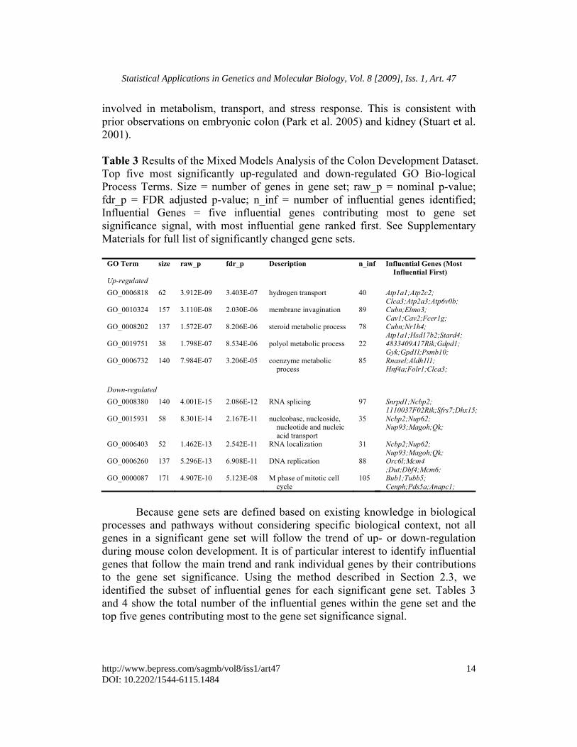
involved in metabolism, transport, and stress response. This is consistent with prior observations on embryonic colon (Park et al. 2005) and kidney (Stuart et al. 2001). Table 3 Results of the Mixed Models Analysis of the Colon Development Dataset. Top five most significantly up-regulated and down-regulated GO Bio-logical Process Terms. Size = number of genes in gene set; raw_p = nominal p-value; fdr_p = FDR adjusted p-value; n_inf = number of influential genes identified; Influential Genes = five influential genes contributing most to gene set significance signal, with most influential gene ranked first. See Supplementary Materials for full list of significantly changed gene sets.

GO Term size raw_p fdr_p Description n_inf Influential Genes (Most Influential First)

Up-regulated GO_0006818 62 3.912E-09 3.403E-07 hydrogen transport 40 Atp1a1;Atp2c2;

Clca3;Atp2a3;Atp6v0b; GO_0010324 157 3.110E-08 2.030E-06 membrane invagination 89 Cubn;Elmo3;

Cav1;Cav2;Fcer1g; GO_0008202 137 1.572E-07 8.206E-06 steroid metabolic process 78 Cubn;Nr1h4;

Atp1a1;Hsd17b2;Stard4; GO_0019751 38 1.798E-07 8.534E-06 polyol metabolic process 22 4833409A17Rik;Gdpd1;

Gyk;Gpd1l;Psmb10; GO_0006732 140 7.984E-07 3.206E-05 coenzyme metabolic

process 85 Rnasel;Aldh1l1;

Hnf4a;Folr1;Clca3; Down-regulated GO_0008380 140 4.001E-15 2.086E-12 RNA splicing 97 Snrpd1;Ncbp2;

1110037F02Rik;Sfrs7;Dhx15; GO_0015931 58 8.301E-14 2.167E-11 nucleobase, nucleoside,

nucleotide and nucleic acid transport

35 Ncbp2;Nup62; Nup93;Magoh;Qk;

GO_0006403 52 1.462E-13 2.542E-11 RNA localization 31 Ncbp2;Nup62; Nup93;Magoh;Qk;

GO_0006260 137 5.296E-13 6.908E-11 DNA replication 88 Orc6l;Mcm4 ;Dut;Dbf4;Mcm6;

GO_0000087 171 4.907E-10 5.123E-08 M phase of mitotic cell cycle

105 Bub1;Tubb5; Cenph;Pds5a;Anapc1;

Because gene sets are defined based on existing knowledge in biological processes and pathways without considering specific biological context, not all genes in a significant gene set will follow the trend of up- or down-regulation during mouse colon development. It is of particular interest to identify influential genes that follow the main trend and rank individual genes by their contributions to the gene set significance. Using the method described in Section 2.3, we identified the subset of influential genes for each significant gene set. Tables 3 and 4 show the total number of the influential genes within the gene set and the top five genes contributing most to the gene set significance signal.

14



4. DISCUSSION In this paper, we have proposed a unified strategy for systems analysis of time course microarray experiments at the gene set level using random coefficient models. Several features of the proposed models make them especially attractive in this setting: First, in the analysis of gene sets, to avoid inflation of false positive rate, great care must be taken to account for correlations between genes in the same pathway. For testing the central null hypothesis, we have shown both theoretically (Section 2.2) and empirically (Section 3.1) that the proposed random coefficient model adequately captures the primary covariance structure between genes and preserves type I error rate. On the other hand, permutation tests rely on exchangeability of the permuted units, careful consideration are required to account for data structure in complex study designs to avoid misleading results (Churchill et al. 2008). For example, Xu and Hsu (2007) showed that when comparing mean expression levels of a set of genes between two groups of subjects, permutation tests based on permuting sample labels across groups may not preserve type I error rate, when the joint distributions of gene expression levels differ between the groups. Second, using gene expression data with “real life” correlations, we have shown in comparison to currently available methods, by modeling the mean trajectory and testing the central hypothesis for a group of genes, the proposed random coefficient models yield statistical inferences for gene sets that are more stable (less affected by sampling variation) and more interpretable (allowing ranking of individual genes that contribute most to the gene set signal). In the analysis of the mouse embryonic colon dataset, the agreement between results of the random coefficient models and previous reports further validates the proposed method. Finally, the proposed method is a general methodology that operates within a well-established statistical framework. This flexible, unified and practical approach can be easily implemented in common statistical software packages. By including design factors and covariate effects, the random coefficient models can be augmented easily to handle more complex designs with multiple sources of variation such as those with biological replicates or even spatial effects. For example, when arrays are processed in multiple batches, a batch effect can be added to the model to adjust for systematic effects from different batches. Similarly, other random effects from blocks and sites where the experiments were performed can also be incorporated into the model. Littell et al. (2006) provides a comprehensive set of examples covering a wide range of mixed models and related covariance structures.

15



REFERENCE Ashburner, M., C.A. Ball, J.A. Blake, D. Botstein, H. Butler, J.M. Cherry, A.P.

Davis, K. Dolinski, S.S. Dwight, J.T. Eppig, M.A. Harris et al. 2000. Gene ontology: tool for the unification of biology. The Gene Ontology Consortium. Nat Genet 25: 25-29.

Barry, W.T., A.B. Nobel, F.A. Wright. 2005. Significance analysis of functional categories in gene expression studies: a structured permutation approach. Bioinformatics 21: 1943-1949.

Chen, X., L. Wang, J.D. Smith, B. Zhang. 2008. Supervised principal component analysis for gene set enrichment of microarray data with continuous or survival outcomes. Bioinformatics 24: 2474-2481.

Chu, T.M., B. Weir, R. Wolfinger. 2002. A systematic statistical linear modeling approach to oligonucleotide array experiments. Math Biosci 176: 35-51.

Churchill, G.A., R.W. Doerge. 2008. Naive application of permutation testing leads to inflated type I error rates. Genetics 178: 609-610.

Dahlquist, K.D., N. Salomonis, K. Vranizan, S.C. Lawlor, B.R. Conklin. 2002. GenMAPP, a new tool for viewing and analyzing microarray data on biological pathways. Nat Genet 31: 19-20.

Draghici, S., P. Khatri, P. Bhavsar, A. Shah, S.A. Krawetz, M.A. Tainsky. 2003. Onto-Tools, the toolkit of the modern biologist: Onto-Express, Onto-Compare, Onto-Design and Onto-Translate. Nucleic Acids Res 31: 3775-3781.

Gentleman, R.C., V.J. Carey, D.M. Bates, B. Bolstad, M. Dettling, S. Dudoit, B. Ellis, L. Gautier, Y. Ge, J. Gentry, K. Hornik et al. 2004. Bioconductor: open software development for computational biology and bioinformatics. Genome Biol 5: R80.

Goeman, J.J., S.A. van de Geer, F. de Kort, H.C. van Houwelingen. 2004. A global test for groups of genes: testing association with a clinical outcome. Bioinformatics 20: 93-99.

Hummel, M., R. Meister, U. Mansmann. 2008. GlobalANCOVA: exploration and assessment of gene group effects. Bioinformatics 24: 78-85.

Irizarry, R.A., B. Hobbs, F. Collin, Y.D. Beazer-Barclay, K.J. Antonellis, U. Scherf, T.P. Speed. 2003. Exploration, normalization, and summaries of high density oligonucleotide array probe level data. Biostatistics 4: 249-264.

Jolliffe, I.T. 2002. Principal Component Analysis. Springer, New York, NY. Kim, S.Y., D.J. Volsky. 2005. PAGE: parametric analysis of gene set enrichment.

BMC Bioinformatics 6: 144. Littell, R.C., G.A. Miliken, W.W. Stroup, R. Wolfinger, O. Schabenberger. 2006.

SAS for Mixed Models. SAS Institute Inc., Cary, NC.

16



Liu, J., J.M. Hughes-Oliver, J.A. Menius, Jr. 2007. Domain-enhanced analysis of microarray data using GO annotations. Bioinformatics 23: 1225-1234.

Luan, Y., H. Li. 2004. Model-based methods for identifying periodically expressed genes based on time course microarray gene expression data. Bioinformatics 20: 332-339.

Mootha, V.K., C.M. Lindgren, K.F. Eriksson, A. Subramanian, S. Sihag, J. Lehar, P. Puigserver, E. Carlsson, M. Ridderstrale, E. Laurila, N. Houstis et al. 2003. PGC-1alpha-responsive genes involved in oxidative phosphorylation are coordinately downregulated in human diabetes. Nat Genet 34: 267-273.

Park, T., S.G. Yi, S. Lee, S.Y. Lee, D.H. Yoo, J.I. Ahn, Y.S. Lee. 2003. Statistical tests for identifying differentially expressed genes in time-course microarray experiments. Bioinformatics 19: 694-703.

Park, Y.K., J.L. Franklin, S.H. Settle, S.E. Levy, E. Chung, L.H. Jeyakumar, Y. Shyr, M.K. Washington, R.H. Whitehead, B.J. Aronow, R.J. Coffey. 2005. Gene expression profile analysis of mouse colon embryonic development. Genesis 41: 1-12.

Storey, J.D., W. Xiao, J.T. Leek, R.G. Tompkins, R.W. Davis. 2005. Significance analysis of time course microarray experiments. Proc Natl Acad Sci U S A 102: 12837-12842.

Stuart, R.O., K.T. Bush, S.K. Nigam. 2001. Changes in global gene expression patterns during development and maturation of the rat kidney. Proc Natl Acad Sci U S A 98: 5649-5654.

Wang, L., B. Zhang, R.D. Wolfinger, X. Chen. 2008. An integrated approach for the analysis of biological pathways using mixed models. PLoS Genet 4: e1000115.

Wolfinger, R.D., G. Gibson, E.D. Wolfinger, L. Bennett, H. Hamadeh, P. Bushel, C. Afshari, R.S. Paules. 2001. Assessing gene significance from cDNA microarray expression data via mixed models. J Comput Biol 8: 625-637.

Xu, H., J.C. Hsu. Using the partition principal to control the generalized family error rate. Biometrical Journal 49: 52-67.

Zhang, B., S. Kirov, J. Snoddy. 2005. WebGestalt: an integrated system for exploring gene sets in various biological contexts. Nucleic Acids Res 33: W741-748.

Zhang, B., D. Schmoyer, S. Kirov, J. Snoddy. 2004. GOTree Machine (GOTM): a web-based platform for interpreting sets of interesting genes using Gene Ontology hierarchies. BMC Bioinformatics 5: 16.

17



statistical applications in genetics and molecular biology · provides a uniﬁed statistical model...

Documents