statistical and numerical methods for chemical...

Statistical and Numerical Methodsfor Chemical Engineers

Part on Statistics

Lukas Meier, ETH Zürich

Lecture Notes of W. Stahel (ETH Zürich) and A. Ruckstuhl (ZHAW)

November 2014

Contents

1 Preliminary Remarks 1

2 Summary of Linear Regression 32.1 Simple Linear Regression . . . . . . . . . . . . . . . . . . . . . . . . . . 32.2 Multiple Linear Regression . . . . . . . . . . . . . . . . . . . . . . . . . 42.3 Residual Analysis . . . . . . . . . . . . . . . . . . . . . . . . . . . . . . . 6

3 Nonlinear Regression 83.1 Introduction . . . . . . . . . . . . . . . . . . . . . . . . . . . . . . . . . . 83.2 Parameter Estimation . . . . . . . . . . . . . . . . . . . . . . . . . . . . 123.3 Approximate Tests and Confidence Intervals . . . . . . . . . . . . . . . . 163.4 More Precise Tests and Confidence Intervals . . . . . . . . . . . . . . . . 203.5 Profile t-Plot and Profile Traces . . . . . . . . . . . . . . . . . . . . . . . 223.6 Parameter Transformations . . . . . . . . . . . . . . . . . . . . . . . . . 243.7 Forecasts and Calibration . . . . . . . . . . . . . . . . . . . . . . . . . . 293.8 Closing Comments . . . . . . . . . . . . . . . . . . . . . . . . . . . . . . 32

4 Analysis of Variance and Design of Experiments 344.1 Multiple Groups, One-Way ANOVA . . . . . . . . . . . . . . . . . . . . 344.2 Random Effects, Ring Trials . . . . . . . . . . . . . . . . . . . . . . . . . 354.3 Two and More Factors . . . . . . . . . . . . . . . . . . . . . . . . . . . . 364.4 Response Surface Methods . . . . . . . . . . . . . . . . . . . . . . . . . . 374.5 Second-Order Response Surfaces . . . . . . . . . . . . . . . . . . . . . . 424.6 Experimental Designs, Robust Designs . . . . . . . . . . . . . . . . . . . 464.7 Further Reading . . . . . . . . . . . . . . . . . . . . . . . . . . . . . . . 46

5 Multivariate Analysis of Spectra 485.1 Introduction . . . . . . . . . . . . . . . . . . . . . . . . . . . . . . . . . . 485.2 Multivariate Statistics: Basics . . . . . . . . . . . . . . . . . . . . . . . . 495.3 Principal Component Analysis (PCA) . . . . . . . . . . . . . . . . . . . 515.4 Linear Mixing Models, Factor Analysis . . . . . . . . . . . . . . . . . . . 565.5 Regression with Many Predictors . . . . . . . . . . . . . . . . . . . . . . 56

I

1 Preliminary Remarks

a Several types of problems lead to statistical models that are highly relevant for chemicalengineers:• A response variable like yield or quality of a product or the duration of a pro-

duction process may be influenced by a number of variables – plausible examplesare temperature, pressure, humidity, properties of the input material (educts).– In a first step, we need a model for describing the relations. This leads

to regression and analysis of variance models. Quite often, simple ormultiple linear regression already give good results.

– Optimization of production processes: If the relations are modelledadequately, it is straightforward to search for those values of the variablesthat drive the response variable to an optimal value. Methods to efficientlyfind these optimum values are discussed under the label of design of ex-periments.

• Chemical processes develop according to clear laws (“law and order of chemicalchange”, Swinbourne, 1971), which are typically modelled by differential equa-tions. In these systems there are constants, like the reaction rates, which can bedetermined from data of suitable experiments. In the simplest cases this leads tolinear regression, but usually, the methods of non-linear regression, possiblycombined with the numerical solution of differential equations, are needed. Wecall this combination system analysis.

• As an efficient surrogate for chemical determination of concentrations of differentcompounds, indirect determination by spectroscopical measurements are oftensuitable. Methods that allow for inferring amounts or concentrations of chemicalcompounds from spectra belong to the field of multivariate statistics.

b In the very limited time available in this course we will present an introduction tothese topics. We start with linear regression, a topic you should already be familiarwith. The simple linear regression model is used to recall basic statistical notions. Thefollowing steps are common for statistical methods:

1. State the scientific question and characterize the data which are available or willbe obtained.

2. Find a suitable probability model that corresponds to the knowledge about theprocesses leading to the data. Typically, a few unknown constants remain, whichwe call “parameters” and which we want to learn from the data. The model can(and should) be formulated before the data is available.

3. The field of statistics encompasses the methods that bridge the gap betweenmodels and data. Regarding parameter values, statistics answers the followingquestions:a) Which value is the most plausible one for a parameter? The answer

is given by estimation. An estimator is a function that determines aparameter value from the data.

b) Is a given value for the parameter plausible? The decision is made by using

1

a statistical test.c) Which values are plausible? The answer is given by a set of all plausible

values, which is usually an interval, the so called confidence interval.4. In many applications the prediction of measurements (observations) that are

not yet available is of interest.

c Linear regression was already discussed in “Grundlagen der Mathematik II”. Pleasehave a look at your notes to (again) get familiar with the topic.You find additional material for this part of the course on

http://stat.ethz.ch/˜meier/teaching/cheming

2 Summary of Linear Regression

2.1 Simple Linear Regression

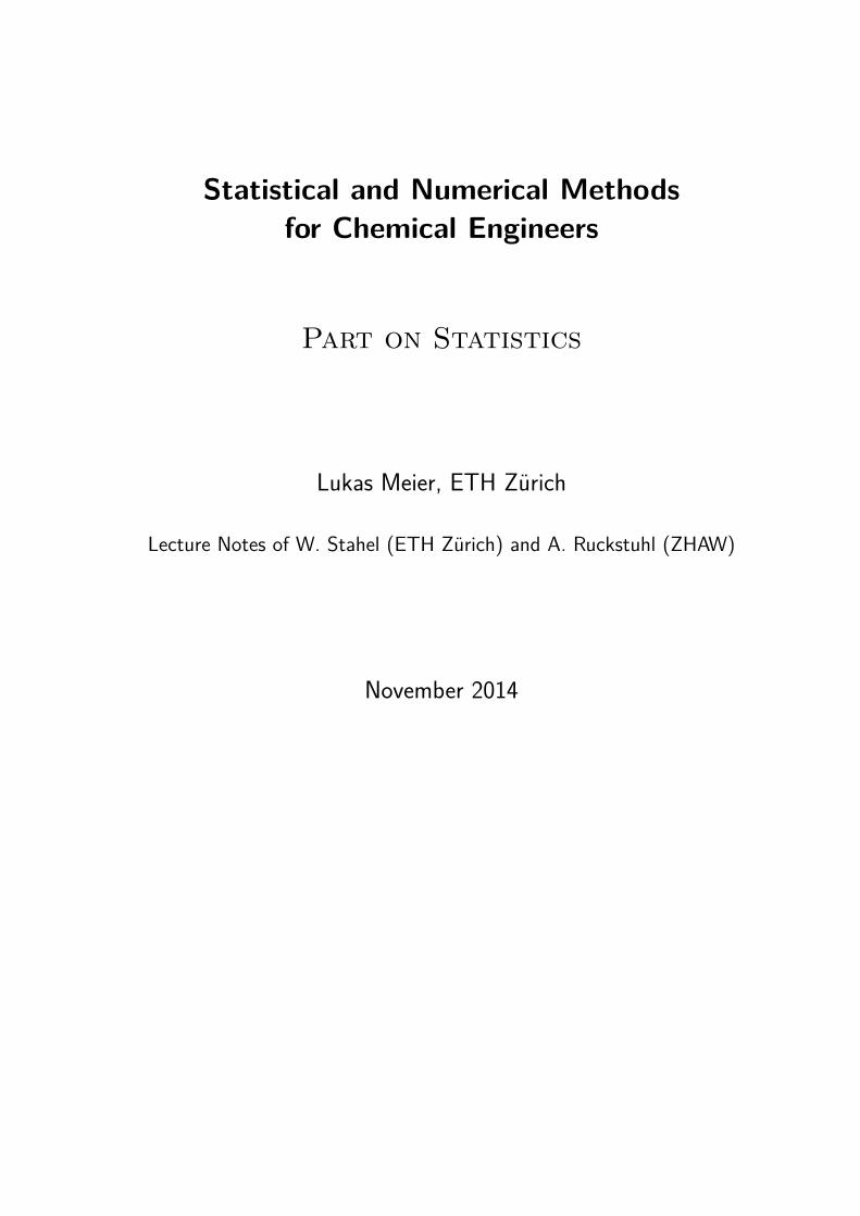
a Assume we have n observations (xi, Yi), i = 1, . . . , n and we want to model therelationship between a response variable Y and a predictor variable x .The simple linear regression model is

Yi = α+ βxi + Ei, i = 1, . . . , n.

The xi ’s are fixed numbers while the Ei ’s are random, called “random deviations” or“random errors”. Usual assumptions are

Ei ∼ N (0, σ2), Ei independent.

The parameters of the simple linear regression model are the coefficients α, β andthe standard deviation σ of the random error.Figure 2.1.a illustrates the model.

b Estimation of the coefficients follows the principle of least squares and yields

β =∑ni=1(Yi − Y )(xi − x)∑n

i=1(xi − x)2 , α = Y − β x .

The estimates β and α fluctuate around the true (but unknown) parameters. Moreprecisely, the estimates are normally distributed,

β ∼ N (β, σ2/SSX) , α ∼ N(α, σ2

(1n + x2/SSX

)),

1.6 1.8 2.0

0

1

x

Y error density

Figure 2.1.a: Display of the probability model Yi = 4− 2xi +Ei for 3 observations Y1 , Y2 andY3 corresponding to the x values x1 = 1.6, x2 = 1.8 and x3 = 2.

3

4 2 Summary of Linear Regression

where SSX =∑ni=1(xi − x)2 .

c The deviations of the observed Yi from the fitted values yi = α + βxi are calledresiduals Ri = Yi − yi and are “estimators” of the random errors Ei .They lead to an estimate of the standard deviation σ of the error,

σ2 = 1n− 2

n∑i=1

R2i .

d Test of the null hypothesis β = β0 : The test statistic

T = β − β0

se(β), se(β) =

√σ2/SSX

has a t-distribution with n− 2 degrees of freedom under the null-hypothesis.This leads to the confidence interval of

β ± qtn−20.975 se(β).

e The “confidence band” for the value of the regression function connects the endpoints of the confidence intervals for E(Y |x) = α+ βx .A prediction interval shall include a (yet unknown) value Y0 of the response variablefor a given x0 – with a given “statistical certainty” (usually 95%). Connecting the endpoints for all possible x0 produces the “prediction band”.

2.2 Multiple Linear Regression

a Compared to the simple linear regression model we now have several predictorsx(1), . . . , x(m) .The multiple linear regression model is

Yi = β0 + β1x(1)i + β2x

(2)i + ...+ βmx

(m)i + Ei

Ei ∼ N (0, σ2), Ei independent.

In matrix notation:

Y = Xβ + E , E ∼ Nn(0, σ2 I ),

where the response vector Y ∈ Rn , the design matrix X ∈ Rn×p , the parametervector β ∈ Rp and the error vector E ∈ Rn for p = m+ 1 (number of parameters).

Y =

Y1Y2...Yn

, X =

1 x

(1)1 x

(2)1 . . . x

(m)1

1 x(1)2 x

(2)2 . . . x

(m)2

......

......

...1 x

(1)n x

(2)n . . . x

(m)n

, β =

β0β1...βm

, E =

E1E2...En

.

Different rows of the design matrix X are different observations. The variables (pre-dictors) can be found in the corresponding columns.

2.2 Multiple Linear Regression 5

b Estimation is again based on least squares, leading to

β = (X T X )−1 X TY ,

i.e. we have a closed form solution.From the distribution of the estimated coefficients,

βj ∼ N(βj , σ

2((X T X )−1

)jj

)t-tests and confidence intervals for individual coefficients can be derived as in the linearregression model. The test statistic

T = βj − βj,0se(βj)

, se(βj) =√σ2((X T X )−1

)jj

follows a t-distribution with n − (m + 1) parameters under the null-hypothesis H0 :βj = βj,0 .The standard deviation σ is estimated by

σ2 = 1n− p

n∑i=1

R2i .

c Table 2.2.c shows a typical computer output, annotated with the correspondingmathematical symbols.The multiple correlation R is the correlation between the fitted values yi and theobserved values Yi . Its square measures the portion of the variance of the Yi ’s that is“explained by the regression”, and is therefore called coefficient of determination:

R2 = 1− SSE/SSY ,

where SSE =∑ni=1(Yi − yi)2, SSY =

∑ni=1(Yi − Y )2 .

Coefficients:Value βj Std. Error t value Pr(>|t|)

(Intercept) 19.7645 2.6339 7.5039 0.0000pH -1.7530 0.3484 -5.0309 0.0000lSAR -1.2905 0.2429 -5.3128 0.0000

Residual standard error: σ = 0.9108 on n− p = 120 degrees of freedomMultiple R-Squared: R2 = 0.5787

Analysis of varianceDf Sum of Sq Mean Sq F Value Pr(F)

Regression m = 2 SSR = 136.772 68.386 T = 82.43 0.0000Residuals n−p = 120 SSE = 99.554 σ2 = 0.830 p-valueTotal 122 SSY = 236.326

Table 2.2.c: Computer output for a regression example, annotated with mathematical symbols.

d

6 2 Summary of Linear Regression

The model is called linear because it is linear in the parameters β0, . . . , βm .It could well be that some predictors are non-linear functions of other predictors (e.g.,x(2) = (x(1))2 ). It is still a linear model as long as the parameters appear in linearform!

e In general, it is not appropriate to replace a multiple regression model by many simpleregressions (on single predictor variables).In a multiple linear regression model, the coefficients describe how Y is changing whenvarying the corresponding predictor and keeping the other predictor variablesconstant. I.e., it is the effect of the predictor on the response after having subtractedthe effect of all other predictors on Y . Hence we need to have all predictors in themodel at the same time in order to estimate this effect.

f Many applications The model of multiple linear regression model is suitable fordescribing many different situations:• Transformations of the predictors (and the response variable) may turn origi-

nally non-linear relations into linear ones.• A comparison of two groups is obtained by using a binary predictor variable.

Several groups need a “block of dummy variables”. Thus, nominal (or cate-gorical) explanatory variables can be used in the model and can be combinedwith continuous variables.

• The idea of different linear relations of the response with some predictors indifferent groups of data can be included into a single model. More generally, in-teractions between explanatory variables can be incorporated by suitable termsin the model.

• Polynomial regression is a special case of multiple linear (!) regression (seeexample above).

g The F-Test for comparison of models allows for testing whether several coefficientsare zero. This is needed for testing whether a categorical variable has an influence onthe response.

2.3 Residual Analysis

a The assumptions about the errors of the regression model can be split into(a) their expected values are zero: E(Ei) = 0 (or: the regression function is

correct),(b) they have constant variance, Var(Ei) = σ2 ,(c) they are normally distributed,(d) they are independent of each other.

These assumptions should be checked for• deriving a better model based on deviations from it,• justifying tests and confidence intervals.

Deviations are detected by inspecting graphical displays. Tests for assumptions playa less important role.

2.3 Residual Analysis 7

b Fitting a regression model without examining the residuals is a risky exer-cise!

c The following displays are useful:(a) Non-linearities: Scatterplot of (unstandardized) residuals against fitted values

(Tukey-Anscombe plot) and against the (original) explanatory variables.Interactions: Pseudo-threedimensional diagram of the (unstandardized) resid-uals against pairs of explanatory variables.

(b) Equal scatter: Scatterplot of (standardized) absolute residuals against fittedvalues (Tukey-Anscombe plot) and against (original) explanatory vari-ables. Usually no special displays are given, but scatter is examined in theplots for (a).

(c) Normal distribution: QQ-plot (or histogram) of (standardized) residuals.(d) Independence: (unstandardized) residuals against time or location.(e) Influential observations for the fit: Scatterplot of (standardized) residuals

against leverage.Influential observations for individual coefficients: added-variable plot.

(f) Collinearities: Scatterplot matrix of explanatory variables and numerical out-put (of R2

j or VIFj or “tolerance”).

d Remedies:• Transformation (monotone non-linear) of the response: if the distribu-

tion of the residuals is skewed, for non-linearities (if suitable) or unequal vari-ances.

• Transformation (non-linear) of explanatory variables: when seeing non-linearities, high leverages (can come from skewed distribution of explanatoryvariables) and interactions (may disappear when variables are transformed).

• Additional terms: to model non-linearities and interactions.• Linear transformations of several explanatory variables: to avoid collinearities.• Weighted regression: if variances are unequal.• Checking the correctness of observations: for all outliers in any display.• Rejection of outliers: if robust methods are not available (see below).

More advanced methods:• Generalized least squares: to account for correlated random errors.• Non-linear regression: if non-linearities are observed and transformations of vari-

ables do not help or contradict a physically justified model.• Robust regression: should always be used, suitable in the presence of outliers

and/or long-tailed distributions.

Note that correlations among errors lead to wrong test results and confidence intervalswhich are most often too short.

3 Nonlinear Regression

3.1 Introduction

a The Regression Model Regression studies the relationship between a variable ofinterest Y and one or more explanatory or predictor variables x(j) . The generalmodel is

Yi = h(x(1)i , x

(2)i , . . . , x

(m)i ; θ1, θ2, . . . , θp) + Ei.

Here, h is an appropriate function that depends on the predictor variables and pa-rameters, that we want to summarize with vectors x = [x(1)

i , x(2)i , . . . , x

(m)i ]T and

θ = [θ1, θ2, . . . , θp]T . We assume that the errors are all normally distributed andindependent, i.e.

Ei ∼ N(0, σ2

), independent.

b The Linear Regression Model In (multiple) linear regression, we considered functionsh that are linear in the parameters θj ,

h(x(1)i , x

(2)i , . . . , x

(m)i ; θ1, θ2, . . . , θp) = θ1x

(1)i + θ2x

(2)i + . . .+ θpx

(p)i ,

where the x(j) can be arbitrary functions of the original explanatory variables x(j) .There, the parameters were usually denoted by βj instead of θj .

c The Nonlinear Regression Model In nonlinear regression, we use functions h thatare not linear in the parameters. Often, such a function is derived from theory. Inprinciple, there are unlimited possibilities for describing the deterministic part of themodel. As we will see, this flexibility often means a greater effort to make statisticalstatements.

Example d Puromycin The speed of an enzymatic reaction depends on the concentration of asubstrate. As outlined in Bates and Watts (1988), an experiment was performed toexamine how a treatment of the enzyme with an additional substance called Puromycininfluences the reaction speed. The initial speed of the reaction is chosen as the responsevariable, which is measured via radioactivity (the unit of the response variable iscount/min2 ; the number of registrations on a Geiger counter per time period measuresthe quantity of the substance, and the reaction speed is proportional to the change pertime unit).The relationship of the variable of interest with the substrate concentration x (in ppm)is described by the Michaelis-Menten function

h(x; θ) = θ1x

θ2 + x.

An infinitely large substrate concentration (x→∞) leads to the “asymptotic” speedθ1 . It was hypothesized that this parameter is influenced by the addition of Puromycin.The experiment is therefore carried out once with the enzyme treated with Puromycin

8

3.1 Introduction 9

0.0 0.2 0.4 0.6 0.8 1.0

50

100

150

200

Concentration

Vel

ocity

Concentration

Vel

ocity

Figure 3.1.d: Puromycin. (a) Data (• treated enzyme; 4 untreated enzyme) and (b) typicalshape of the regression function.

1 2 3 4 5 6 7

8

10

12

14

16

18

20

Days

Oxy

gen

Dem

and

Days

Oxy

gen

Dem

and

Figure 3.1.e: Biochemical Oxygen Demand. (a) Data and (b) typical shape of the regressionfunction.

and once with the untreated enzyme. Figure 3.1.d shows the data and the shape ofthe regression function. In this section only the data of the treated enzyme is used.

Example e Biochemical Oxygen Demand To determine the biochemical oxygen demand, streamwater samples were enriched with soluble organic matter, with inorganic nutrientsand with dissolved oxygen, and subdivided into bottles (Marske, 1967, see Bates andWatts, 1988). Each bottle was inoculated with a mixed culture of microorganisms,sealed and put in a climate chamber with constant temperature. The bottles wereperiodically opened and their dissolved oxygen concentration was analyzed, from whichthe biochemical oxygen demand [mg/l] was calculated. The model used to connect thecumulative biochemical oxygen demand Y with the incubation time x is based onexponential decay:

h(x; θ) = θ1(1− e−θ2x

).

Figure 3.1.e shows the data and the shape of the regression function.

10 3 Nonlinear Regression

2 4 6 8 10 12

160

161

162

163

x (=pH)

y (=

che

m. s

hift)

(a)

x

y

(b)

Figure 3.1.f: Membrane Separation Technology. (a) Data and (b) a typical shape of the regres-sion function.

Example f Membrane Separation Technology See Rapold-Nydegger (1994). The ratio of proto-nated to deprotonated carboxyl groups in the pores of cellulose membranes depends onthe pH-value x of the outer solution. The protonation of the carboxyl carbon atomscan be captured with 13 C-NMR. We assume that the relationship can be written withthe extended “Henderson-Hasselbach Equation” for polyelectrolytes

log10

(θ1 − yy − θ2

)= θ3 + θ4 x ,

where the unknown parameters are θ1, θ2 and θ3 > 0 and θ4 < 0. Solving for y leadsto the model

Yi = h(xi; θ) + Ei = θ1 + θ2 10θ3+θ4xi

1 + 10θ3+θ4xi+ Ei .

The regression function h(xi, θ) for a reasonably chosen θ is shown in Figure 3.1.f nextto the data.

g A Few Further Examples of Nonlinear Regression Functions• Hill model (enzyme kinetics): h(xi, θ) = θ1x

θ3i /(θ2 + xθ3

i )For θ3 = 1 this is also known as the Michaelis-Menten model (3.1.d).

• Mitscherlich function (growth analysis): h(xi, θ) = θ1 + θ2 exp(θ3xi).• From kinetics (chemistry) we get the function

h(x(1)i , x

(2)i ; θ) = exp(−θ1x

(1)i exp(−θ2/x

(2)i )).

• Cobbs-Douglas production function

h(x

(1)i , x

(2)i ; θ

)= θ1

(x

(1)i

)θ2 (x

(2)i

)θ3.

Since useful regression functions are often derived from the theoretical background ofthe application of interest, a general overview of nonlinear regression functions is ofvery limited benefit. A compilation of functions from publications can be found inAppendix 7 of Bates and Watts (1988).

h Linearizable Regression Functions Some nonlinear regression functions can be lin-earized by transformations of the response variable and the explanatory variables.

3.1 Introduction 11

For example, a power functionh(x; θ) = θ1x

θ2

can be transformed to a linear (in the parameters!) function

ln(h(x; θ)) = ln(θ1) + θ2 ln(x) = β0 + β1x ,

where β0 = ln(θ1), β1 = θ2 and x = ln(x). We call the regression function hlinearizable, if we can transform it into a function that is linear in the (unknown)parameters by (monotone) transformations of the arguments and the response.

Here are some more linearizable functions (see also Daniel and Wood, 1980):

h(x; θ) = 1/(θ1 + θ2 exp(−x)) ←→ 1/h(x; θ) = θ1 + θ2 exp(−x)

h(x; θ) = θ1x/(θ2 + x) ←→ 1/h(x; θ) = 1/θ1 + θ2/θ11x

h(x; θ) = θ1xθ2 ←→ ln(h(x; θ)) = ln(θ1) + θ2 ln(x)

h(x; θ) = θ1 exp(θ2g(x)) ←→ ln(h(x; θ)) = ln(θ1) + θ2g(x)

h(x; θ) = exp(−θ1x(1) exp(−θ2/x

(2))) ←→ ln(ln(h(x; θ))) = ln(−θ1) + ln(x(1))− θ2/x(2)

h(x; θ) = θ1(x(1))θ2 (

x(2))θ3 ←→ ln(h(x; θ)) = ln(θ1) + θ2 ln(x(1)) + θ3 ln(x(2)) .

The last one is the Cobbs-Douglas Model from 3.1.g.

i A linear regression with the linearized regression function of the example above isbased on the model

ln(Yi) = β0 + β1xi + Ei ,

where the random errors Ei all have the same normal distribution. We transform thismodel back and get

Yi = θ1 · xθ2 · Ei,

with Ei = exp(Ei). The errors Ei , i = 1, . . . , n , now have a multiplicative effect andare log-normally distributed! The assumptions about the random deviations are thusnow drastically different than for a model that is based directly on h ,

Yi = θ1 · xθ2 + E∗i ,

with random deviations E∗i that, as usual, contribute additively and have a specificnormal distribution.

A linearization of the regression function is therefore advisable only if the assumptionsabout the random errors can be better satisfied – in our example, if the errors actuallyact multiplicatively rather than additively and are log-normally rather than normallydistributed. These assumptions must be checked with residual analysis.

j * Note: For linear regression it can be shown that the variance can be stabilized with certain trans-formations (e.g. log(·),

√·). If this is not possible, in certain circumstances one can also perform a

weighted linear regression. The process is analogous in nonlinear regression.


k We have almost exclusively seen regression functions that only depend on one predictorvariable x . This was primarily because it was possible to graphically illustrate themodel. The following theory also works well for regression functions h(x; θ) thatdepend on several predictor variables x = [x(1), x(2), . . . , x(m)] .

3.2 Parameter Estimation

a The Principle of Least Squares To get estimates for the parameters θ = [θ1 , θ2 , . . . ,θp]T , one applies – like in linear regression – the principle of least squares. The sumof the squared deviations

S(θ) :=n∑i=1

(yi − ηi(θ))2 where ηi(θ) := h(xi; θ)

should be minimized. The notation that replaces h(xi; θ) with ηi(θ) is reasonablebecause [xi, yi] is given by the data and only the parameters θ remain to be determined.Unfortunately, the minimum of S(θ) and hence the estimator have no explicit solu-tion (in contrast to the linear regression case). Iterative numeric procedures aretherefore needed. We will sketch the basic ideas of the most common algorithm. It isalso the basis for the easiest way to derive tests and confidence intervals.

b Geometrical Illustration The observed values Y = [Y1, Y2, . . . , Yn]T define a pointin n-dimensional space. The same holds true for the “model values” η (θ) =[η1 (θ) , η2 (θ) , . . . , ηn (θ)]T for a given θ .Please take note: In multivariate statistics where an observation consists of m variablesx(j) , j = 1, 2, . . . ,m , it’s common to illustrate the observations in the m-dimensionalspace. Here, we consider the Y - and η -values of all n observations as points in then-dimensional space.Unfortunately, geometrical interpretation stops with three dimensions (and thus withthree observations). Nevertheless, let us have a look at such a situation, first for simplelinear regression.

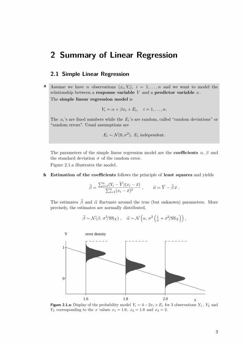
c As stated above, the observed values Y = [Y1, Y2, Y3]T determine a point in three-dimensional space. For given parameters β0 = 5 and β1 = 1 we can calculate the modelvalues ηi

(β)

= β0 + β1xi and represent the corresponding vector η(β)

= β01 + β1x

as a point. We now ask: Where are all the points that can be achieved by varyingthe parameters? These are the possible linear combinations of the two vectors 1and x : they form a plane “spanned by 1 and x”. By estimating the parametersaccording to the principle of least squares, the squared distance between Y and η

(β)

is minimized. This means that we are looking for the point on the plane that isclosest to Y . This is also called the projection of Y onto the plane. The parametervalues that correspond to this point η are therefore the estimated parameter valuesβ = [β0, β1]T . An illustration can be found in Figure 3.2.c.

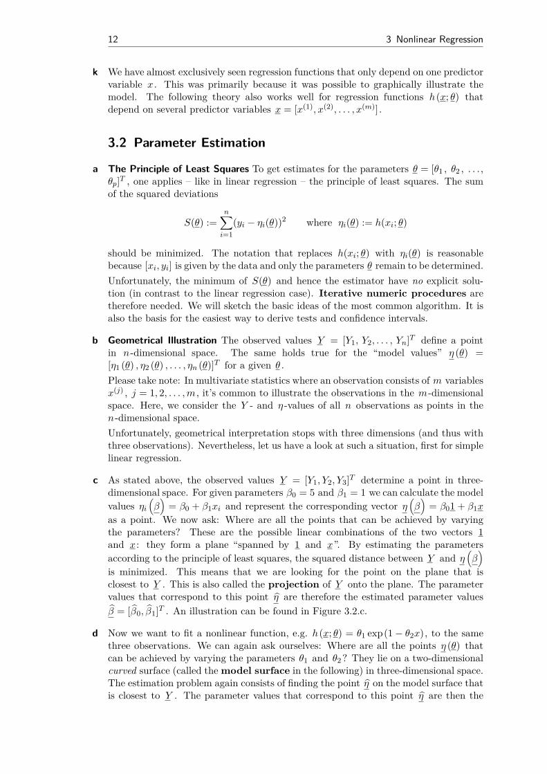
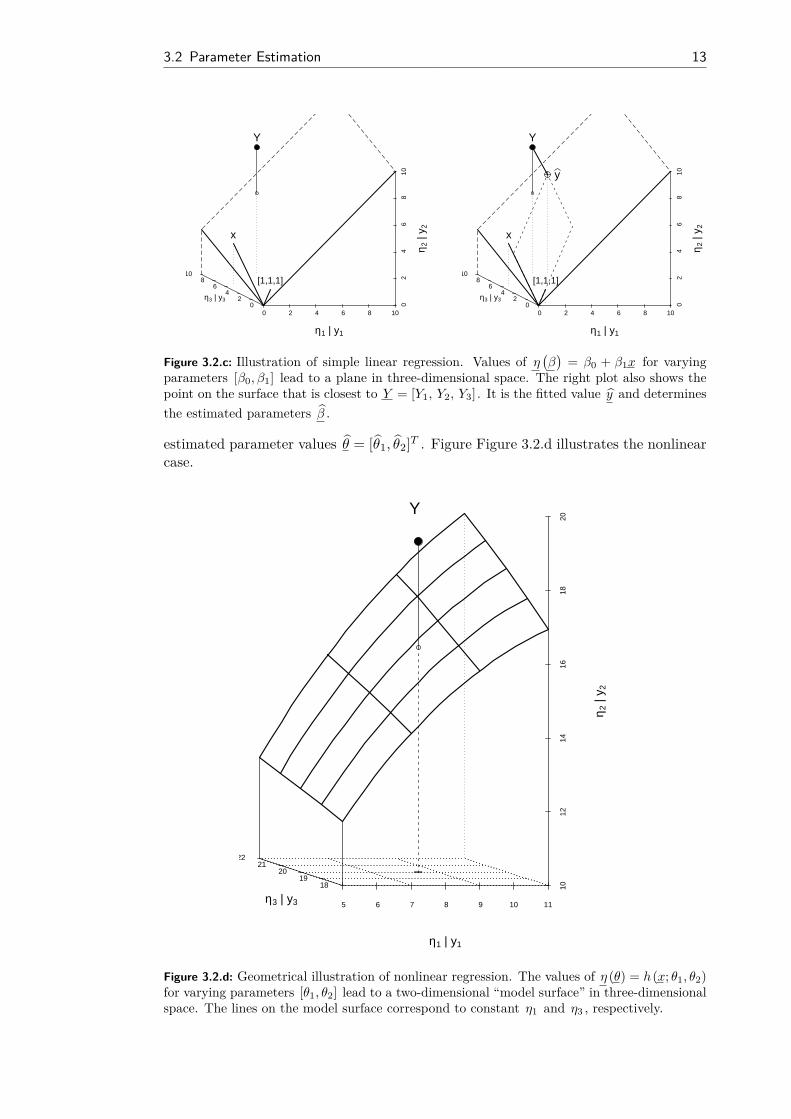
d Now we want to fit a nonlinear function, e.g. h(x; θ) = θ1 exp(1− θ2x), to the samethree observations. We can again ask ourselves: Where are all the points η (θ) thatcan be achieved by varying the parameters θ1 and θ2 ? They lie on a two-dimensionalcurved surface (called the model surface in the following) in three-dimensional space.The estimation problem again consists of finding the point η on the model surface thatis closest to Y . The parameter values that correspond to this point η are then the

3.2 Parameter Estimation 13

0 2 4 6 8 10

0 2

4 6

810

0 2

4 6

810

η1 | y1

η 2 |

y 2

η3 | y3

Y

[1,1,1]

x

0 2 4 6 8 10

0 2

4 6

810

0 2

4 6

810

η1 | y1

η 2 |

y 2

η3 | y3

Y

[1,1,1]

x

y

Figure 3.2.c: Illustration of simple linear regression. Values of η(β)

= β0 + β1x for varyingparameters [β0, β1] lead to a plane in three-dimensional space. The right plot also shows thepoint on the surface that is closest to Y = [Y1, Y2, Y3] . It is the fitted value y and determinesthe estimated parameters β .

estimated parameter values θ = [θ1, θ2]T . Figure Figure 3.2.d illustrates the nonlinearcase.

5 6 7 8 9 10 11

1012

1416

1820

1819

2021

22

η1 | y1

η 2 |

y 2

η3 | y3

−

Y

Figure 3.2.d: Geometrical illustration of nonlinear regression. The values of η (θ) = h(x; θ1, θ2)for varying parameters [θ1, θ2] lead to a two-dimensional “model surface” in three-dimensionalspace. The lines on the model surface correspond to constant η1 and η3 , respectively.


e Biochemical Oxygen Demand (cont’d) The situation for our Biochemical OxygenDemand example can be found in Figure 3.2.e. Basically, we can read the estimatedparameters directly off the graph here: θ1 is a bit less than 21 and θ2 is a bit largerthan 0.6. In fact the (exact) solution is θ = [20.82, 0.6103] (note that these are theparameter estimates for the reduced data set only consisting of three observations).

5 6 7 8 9 10 11

1012

1416

1820

1819

2021

22

η1 | y1

η 2 |

y 2η3 | y3

−

Y

θ1 = 20

θ1 = 21

θ1 = 22

0.3

0.4

0.5θ2 =

−

y

Figure 3.2.e: Biochemical Oxygen Demand: Geometrical illustration of nonlinear regression.In addition, we can see here the lines of constant θ1 and θ2 , respectively. The vector of theestimated model values y = h

(x; θ)

is the point on the model surface that is closest to Y .

f Approach for the Minimization Problem The main idea of the usual algorithm forminimizing the sum of squares (see 3.2.a) is as follows: If a preliminary best value θ(`)

exists, we approximate the model surface with the plane that touches the surface atthe point η

(θ(`)

)= h

(x; θ(`)

)(the so called tangent plane). Now, we are looking for

the point on that plane that lies closest to Y . This is the same as estimation in alinear regression problem. This new point lies on the plane, but not on the surfacethat corresponds to the nonlinear problem. However, it determines a parameter vectorθ(`+1) that we use as starting value for the next iteration.

g Linear Approximation To determine the tangent plane we need the partial derivatives

A(j)i (θ) := ∂ηi (θ)

∂θj,

that can be summarized by an n × p matrix A . The approximation of the model

3.2 Parameter Estimation 15

surface η(θ) by the tangent plane at a parameter value θ∗ is

ηi(θ) ≈ ηi(θ∗) +A(1)i (θ∗) (θ1 − θ∗1) + ...+A

(p)i (θ∗) (θp − θ∗p)

or, in matrix notation,η(θ) ≈ η(θ∗) + A (θ∗) (θ − θ∗) .

If we now add a random error, we get a linear regression model

Y = A (θ∗)β + E

with “preliminary residuals” Y i = Yi − ηi (θ∗) as response variable, the columns of Aas predictors and the coefficients βj = θj − θ∗j (a model without intercept β0 ).

h Gauss-Newton Algorithm The Gauss-Newton algorithm starts with an initial valueθ(0) for θ , solving the just introduced linear regression problem for θ∗ = θ(0) to find acorrection β and hence an improved value θ(1) = θ(0) + β . Again, the approximatedmodel is calculated, and thus the “preliminary residuals” Y − η

(θ(1)

)and the partial

derivatives A(θ(1)

)are determined, leading to θ2 . This iteration step is continued

until the the correction β is small enough.It can not be guaranteed that this procedure actually finds the minimum of the sumof squares. The better the p-dimensional model surface can be locally approximatedby a p-dimensional plane at the minimum θ = (θ1, . . . , θp)T and the closer the initialvalue θ(0) is to the solution, the higher are the chances of finding the optimal value.* Algorithms usually determine the derivative matrix A numerically. In more complex problems the

numerical approximation can be insufficient and cause convergence problems. For such situationsit is an advantage if explicit expressions for the partial derivatives can be used to determine thederivative matrix more reliably (see also Chapter 3.6).

i Initial Values An iterative procedure always requires an initial value. Good initialvalues help to find a solution more quickly and more reliably. Some possibilities toarrive at good initial values are now being presented.

j Initial Value from Prior Knowledge As already noted in the introduction, nonlinearmodels are often based on theoretical considerations of the corresponding applicationarea. Already existing prior knowledge from similar experiments can be used to getan initial value. To ensure the quality of the chosen initial value, it is advisable tographically represent the regression function h(x; θ) for various possible initial valuesθ = θ0 together with the data (e.g., as in Figure 3.2.k, right).

k Initial Values via Linearizable Regression Functions Often – because of the distri-bution of the error term – one is forced to use a nonlinear regression function eventhough it would be linearizable. However, the linearized model can be used to getinitial values.In the Puromycin example the regression function is linearizable: The reciprocal valuesof the two variables fulfill

y = 1y≈ 1h(x; θ) = 1

θ1+ θ2θ1

1x

= β0 + β1x .

The least squares solution for this modified problem is β = [β0, β1]T = (0.00511, 0.000247)T(Figure 3.2.k, left). This leads to the initial values

θ(0)1 = 1/β0 = 196, θ

(0)2 = β1/β0 = 0.048.


0 10 20 30 40 50

0.005

0.010

0.015

0.020

1/Concentration

1/ve

loci

ty

0.0 0.2 0.4 0.6 0.8 1.0

50

100

150

200

Concentration

Vel

ocity

Figure 3.2.k: Puromycin. Left: Regression function in the linearized problem. Right: Regres-sion function h(x; θ) for the initial values θ = θ(0) ( ) and for the least squares estimationθ = θ (——–).

l Initial Values via Geometric Interpretation of the Parameter It is often helpful toconsider the geometrical features of the regression function.In the Puromycin Example we can derive an initial value in another way: θ1 is theresponse value for x =∞ . Since the regression function is monotonically increasing, wecan use the maximal yi -value or a visually determined “asymptotic value” θ

(0)1 = 207

as initial value for θ1 . The parameter θ2 is the x-value, such that y reaches half ofthe asymptotic value θ1 . This leads to θ

(0)2 = 0.06.

The initial values thus result from a geometrical interpretation of the parameters anda rough estimate can be determined by “fitting by eye”.

Example m Membrane Separation Technology (cont’d) In the Membrane Separation Technologyexample we let x→∞ , so h(x; θ) → θ1 (since θ4 < 0); for x→ −∞ , h(x; θ) → θ2 .From Figure 3.1.f (a) we see that θ1 ≈ 163.7 and θ2 ≈ 159.5. Once we know θ1 andθ2 , we can linearize the regression function by

y := log10

(θ

(0)1 − yy − θ(0)

2

)= θ3 + θ4x .

This is called a conditional linearizable function. The linear regression model leadsto the initial value θ(0)

3 = 1.83 and θ(0)4 = −0.36.

With this initial value the algorithm converges to the solution θ1 = 163.7, θ2 = 159.8,θ3 = 2.675 and θ4 = −0.512. The functions h(·; θ(0)) and h(·; θ) are shown in Figure3.2.m (b).* The property of conditional linearity of a function can also be useful to develop an algorithm

specifically suited for this situation (see e.g. Bates and Watts, 1988).

3.3 Approximate Tests and Confidence Intervals

a The estimator θ is the value of θ that optimally fits the data. We now ask whichparameter values θ are compatible with the observations. The confidence region isthe set of all these values. For an individual parameter θj the confidence region is aconfidence interval.

3.3 Approximate Tests and Confidence Intervals 17

2 4 6 8 10 12

−2

−1

0

1

2

x (=pH)

y

(a)

2 4 6 8 10 12

160

161

162

163

x (=pH)

y (=

Ver

schi

ebun

g)

(b)

Figure 3.2.m: Membrane Separation Technology. (a) Regression line that is used for deter-mining the initial values for θ3 and θ4 . (b) Regression function h(x; θ) for the initial valueθ = θ(0) ( ) and for the least squares estimator θ = θ (——–).

The following results are based on the fact that the estimator θ is asymptotically (mul-tivariate) normally distributed. For an individual parameter that leads to a “Z -Test”and the corresponding confidence interval; for multiple parameters the correspondingChi-Square test is used and leads to elliptical confidence regions.

b The asymptotic properties of the estimator can be derived from the linear approx-imation. The problem of nonlinear regression is indeed approximately equal to thelinear regression problem mentioned in 3.2.g

Y = A (θ∗)β + E ,

if the parameter vector θ∗ that is used for the linearization is close to the solution. Ifthe estimation procedure has converged (i.e. θ∗ = θ ), then β = 0 (otherwise this wouldnot be the solution). The standard error of the coefficients β – or more generally thecovariance matrix of β – then approximate the corresponding values of θ .

c Asymptotic Distribution of the Least Squares Estimator It follows that the leastsquares estimator θ is asymptotically normally distributed

θas.∼ N (θ, V (θ)) ,

with asymptotic covariance matrix V (θ) = σ2(A (θ)T A (θ))−1 , where A (θ) is then× p matrix of partial derivatives (see 3.2.g).To explicitly determine the covariance matrix V (θ), A (θ) is calculated using θ insteadof the unknown θ . For the error variance σ2 we plug-in the usual estimator

V (θ) = σ2(

A(θ)T

A(θ))−1

where

σ2 = S(θ)n− p

= 1n− p

n∑i=1

(yi − ηi

(θ) )2

.

Hence, the distribution of the estimated parameters is approximately determined andwe can (like in linear regression) derive standard errors and confidence intervals, orconfidence ellipses (or ellipsoids) if multiple variables are considered jointly.


The denominator n−p in the estimator σ2 was already introduced in linear regressionto ensure that the estimator is unbiased. Tests and confidence intervals were not basedon the normal and Chi-square distribution but on the t- and F-distribution. Theytake into account that the estimation of σ2 causes additional random fluctuation. Evenif the distributions are no longer exact, the approximations are more exact if we do thisin nonlinear regression too. Asymptotically, the difference between the two approachesgoes to zero.

Example d Membrane Separation Technology (cont’d) A computer output for the MembraneSeparation Technology example can be found in Table 3.3.d. The parameter esti-mates are in column Estimate, followed by the estimated approximate standard er-ror (Std. Error) and the test statistics (t value), that are approximately tn−p dis-tributed. The corresponding p-values can be found in column Pr(>|t|). The esti-mated standard deviation σ of the random error Ei is here labelled as “Residualstandard error”.As in linear regression, we can now construct (approximate) confidence intervals. The95% confidence interval for the parameter θ1 is

163.706± qt350.975 · 0.1262 = 163.706± 0.256.

Formula: delta ∼ (T1 + T2 * 10ˆ(T3 + T4 * pH)) / (10ˆ(T3 + T4 * pH) + 1)

Parameters:Estimate Std. Error t value Pr(> |t|)

T1 163.7056 0.1262 1297.256 < 2e-16T2 159.7846 0.1594 1002.194 < 2e-16T3 2.6751 0.3813 7.015 3.65e-08T4 -0.5119 0.0703 -7.281 1.66e-08

Residual standard error: 0.2931 on 35 degrees of freedom

Number of iterations to convergence: 7Achieved convergence tolerance: 5.517e-06

Table 3.3.d: Summary of the fit of the Membrane Separation Technology example.

Example e Puromycin (cont’d) In order to check the influence of treating an enzyme withPuromycin a general model for the data (with and without treatment) can be for-mulated as follows:

Yi = (θ1 + θ3zi)xiθ2 + θ4zi + xi

+ Ei,

where z is the indicator variable for the treatment (zi = 1 if treated, zi = 0 otherwise).Table 3.3.e shows that the parameter θ4 is not significantly different from 0 at the 5%level since the p-value of 0.167 is larger then the level (5%). However, the treatmenthas a clear influence that is expressed through θ3 ; the 95% confidence interval coversthe region 52.398±9.5513 ·2.09 = [32.4, 72.4] (the value 2.09 corresponds to the 97.5%quantile of the t19 distribution).

3.3 Approximate Tests and Confidence Intervals 19

Formula: velocity ∼ (T1 + T3 * (treated == T)) * conc/(T2 + T4 * (treated== T) + conc)


T1 160.280 6.896 23.242 2.04e-15T2 0.048 0.008 5.761 1.50e-05T3 52.404 9.551 5.487 2.71e-05T4 0.016 0.011 1.436 0.167



Table 3.3.e: Computer output of the fit for the Puromycin example.

f Confidence Intervals for Function Values Besides the parameters, the function valueh(x0, θ) for a given x0 is often of interest. In linear regression the function valueh(x0, β

)= xT0 β =: η0 is estimated by η0 = xT0 β and the corresponding (1 − α)

confidence interval isη0 ± q

tn−p1−α/2 · se(η0)

wherese(η0) = σ

√xT0 (X T X )−1x0.

Using asymptotic approximations, we can specify confidence intervals for the func-tion values h(x0; θ) for nonlinear h . If the function η0

(θ)

:= h(x0, θ

)is linearly

approximated at θ we get

η0(θ) ≈ η0(θ) + aT0 (θ − θ) where a0 = ∂h(x0, θ)∂θ

.

If x0 is equal to an observed xi , a0 equals the corresponding row of the matrix Afrom 3.2.g. The (1− α) confidence interval for the function value η0 (θ) := h(x0, θ) isthen approximately

η0(θ)± qtn−p

1−α/2 · se(η0(θ)),

wherese(η0(θ))

= σ

√a T0

(A(θ)T

A(θ) )−1

a0.

Again, the unknown parameter values are replaced by the corresponding estimates.

g Confidence Band The expression for the (1 − α) confidence interval for η0(θ) :=h(x0, θ) also holds for arbitrary x0 . As in linear regression, it is illustrative to representthe limits of these intervals as a “confidence band” that is a function of x0 . See Figure3.3.g for the confidence bands for the examples “Puromycin” and “Biochemical OxygenDemand”.Confidence bands for linear and nonlinear regression functions behave differently: Forlinear functions the confidence band has minimal width at the center of gravity of thepredictor variables and gets wider the further away one moves from the center (seeFigure 3.3.g, left). In the nonlinear case, the bands can have arbitrary shape. Becausethe functions in the “Puromycin” and “Biochemical Oxygen Demand” examples mustgo through zero, the interval shrinks to a point there. Both models have a horizontalasymptote and therefore the band reaches a constant width for large x (see Figure3.3.g, right).


1.0 1.2 1.4 1.6 1.8 2.0 2.2

0

1

2

3

Years^(1/3)

log(

PC

B C

once

ntra

tion)

0 2 4 6 8

0

5

10

15

20

25

30

Days

Oxy

gen

Dem

and

Figure 3.3.g: Left: Confidence band for an estimated line for a linear problem. Right: Confi-dence band for the estimated curve h(x, θ) in the oxygen demand example.

h Prediction Interval The confidence band gives us an idea of the function values h(x)(the expected values of Y for a given x). However, it does not answer the questionwhere future observations Y0 for given x0 will lie. This is often more interestingthan the question of the function value itself; for example, we would like to know wherethe measured value of oxygen demand will lie for an incubation time of 6 days.Such a statement is a prediction about a random variable and should be distinguishedfrom a confidence interval, which says something about a parameter, which is a fixed(but unknown) number. Hence, we call the region prediction interval or prognosisinterval. More about this in Chapter 3.7.

i Variable Selection In nonlinear regression, unlike in linear regression, variable selectionis usually not an important topic, because• there is no one-to-one relationship between parameters and predictor variables.

Usually, the number of parameters is different than the number of predictors.• there are seldom problems where we need to clarify whether an explanatory

variable is necessary or not – the model is derived from the underlying theory(e.g., “enzyme kinetics”).

However, there is sometimes the reasonable question whether a subset of the parame-ters in the nonlinear regression model can appropriately describe the data (see example“Puromycin”).

3.4 More Precise Tests and Confidence Intervals

a The quality of the approximate confidence region that we have seen so far stronglydepends on the quality of the linear approximation. Also, the convergence propertiesof the optimization algorithm are influenced by the quality of the linear approximation.With a somewhat larger computational effort we can check the linearity graphicallyand – at the same time – we can derive more precise confidence intervals.

3.4 More Precise Tests and Confidence Intervals 21

190 200 210 220 230 240

0.04

0.05

0.06

0.07

0.08

0.09

0.10

θ1

θ2

0 10 20 30 40 50 60

0

2

4

6

8

10

θ1

θ2

Figure 3.4.c: Nominal 80 and 95% likelihood contours (——) and the confidence ellipses fromthe asymptotic approximation (– – – –). + denotes the least squares solution. In the Puromycinexample (left) the agreement is good and in the oxygen demand example (right) it is bad.

b F-Test for Model Comparison To test a null hypothesis θ = θ∗ for the whole parametervector or also θj = θ∗j for an individual component, we can use an F -test for modelcomparison like in linear regression. Here, we compare the sum of squares S(θ∗) thatarises under the null hypothesis with the sum of squares S(θ) (for n→∞ the F - testis the same as the so-called likelihood-ratio test, and the sum of squares is, up to aconstant, equal to the negative log-likelihood).Let us first consider a null-hypothesis θ = θ∗ for the whole parameter vector. The teststatistic is

T = n− pp

S(θ∗)− S(θ)S(θ)

(as.)∼ Fp,n−p.

Searching for all null-hypotheses that are not rejected leads us to the confidence region{θ∣∣∣S(θ) ≤ S(θ)

(1 + p

n−p q)}

,

where q = qFp,n−p1−α is the (1 − α) quantile of the F -distribution with p and n − p

degrees of freedom.In linear regression we get the same (exact) confidence region if we use the (multi-variate) normal distribution of the estimator β . In the nonlinear case the results aredifferent. The region that is based on the F -test is not based on the linear approxi-mation in 3.2.g and hence is (much) more exact.

c Confidence Regions for p=2 For p = 2, we can find the confidence regions by cal-culating S(θ) on a grid of θ values and determine the borders of the region throughinterpolation, as is common for contour plots. Figure 3.4.c illustrates both the con-fidence region based on the linear approximation and based on the F -test for theexample “Puromycin” (left) and for “Biochemical Oxygen Demand” (right).For p > 2 contour plots do not exist. In the next chapter we will introduce graphicaltools that also work in higher dimensions. They depend on the following concepts.


d F-Test for Individual Parameters Now we focus on the the question whether an indi-vidual parameter θk is equal to a certain value θ∗k . Such a null hypothesis makes nostatement about the remaining parameters. The model that fits the data best for afixed θk = θ∗k is given by the least squares solution of the remaining parameters. So,S (θ1, . . . , θ

∗k, . . . , θp) is minimized with respect to θj , j 6= k . We denote the minimum

by Sk and the minimizer θj by θj . Both values depend on θ∗k . We therefore writeSk (θ∗k) and θj (θ∗k).The test statistic for the F -test (with null hypothesis H0 : θk = θ∗k ) is given by

T k = (n− p)Sk (θ∗k)− S

(θ)

S(θ) .

It follows (approximately) an F1,n−p distribution.We can now construct a confidence interval by (numerically) solving the equationT k = q

F1,n−p0.95 for θ∗k . It has a solution that is less than θk and one that is larger.

e t-Test via F-Test In linear regression and in the previous chapter we have calculatedtests and confidence intervals from a test value that follows a t-distribution (t-test forthe coefficients). Is this another test?It turns out that the test statistic of the t-test in linear regression turns into the teststatistic of the F -test if we square it. Hence, both tests are equivalent. In nonlinearregression, the F -test is not equivalent to the t-test discussed in the last chapter(3.3.d). However, we can transform the F -test to a t-test that is more accurate thanthe one of the last chapter (that was based on the linear approximation):From the test statistic of the F -test, we take the square-root and add the sign ofθk − θ∗k ,

Tk (θ∗k) := sign(θk − θ∗k

) √Sk(θ∗k)− S

(θ)

σ.

Here, sign(a) denotes the sign of a and as earlier, σ2 = S(θ)/(n − p). This test

statistic is (approximately) tn−p distributed.In the linear regression model, Tk is – as already pointed out – equal to the teststatistic of the usual t-test,

Tk (θ∗k) = θk − θ∗kse(θk) .

f Confidence Intervals for Function Values via F -test With this technique we canalso determine confidence intervals for a function value at a point x0 . For this we re-parameterize the original problem so that a parameter, say φ1 , represents the functionvalue h(x0) and proceed as in 3.4.d.

3.5 Profile t-Plot and Profile Traces

a Profile t-Function and Profile t-Plot The graphical tools for checking the linear ap-proximation are based on the just discussed t-test, that actually doesn’t use thisapproximation. We consider the test statistic Tk (3.4.e) as a function of its argumentsθk and call it profile t-function (in the last chapter the arguments were denotedwith θ∗k , now for simplicity we leave out the ∗ ). For linear regression we get, as can be

3.5 Profile t-Plot and Profile Traces 23

seen from 3.4.e, a straight line, while for nonlinear regression the result is a monotoneincreasing function. The graphical comparison of Tk(θk) with a straight line is theso-called profile t-plot. Instead of θk , it is common to use a standardized version

δk (θk) := θk − θkse(θk)

on the horizontal axis because it is used in the linear approximation. The comparisonline is then the “diagonal”, i.e. the line with slope 1 and intercept 0.The more the profile t-function is curved, the stronger the nonlinearity in a neighbor-hood of θk . Therefore, this representation shows how good the linear approximationis in a neighborhood of θk (the neighborhood that is statistically important is ap-proximately determined by |δk(θk)| ≤ 2.5). In Figure 3.5.a it is evident that in thePuromycin example the nonlinearity is minimal, while in the Biochemical OxygenDemand example it is large.In Figure 3.5.a we can also read off the confidence intervals according to 3.4.e. For con-venience, the probabilites P (Tk ≤ t) of the corresponding t-distributions are markedon the right vertical axis. For the Biochemical Oxygen Demand example this resultsin a confidence interval without upper bound!

b Likelihood Profile Traces The likelihood profile traces are another useful graphicaltool. Here the estimated parameters θj , j 6= k for fixed θk (see 3.4.d) are consideredas functions θ(k)

j (θk).The graphical representation of these functions would fill a whole matrix of diagrams,but without diagonals. It is worthwhile to combine the “opposite” diagrams of thismatrix: Over the representation of θ(k)

j (θk) we superimpose θ(j)k (θj) in mirrored form

so that the axes have the same meaning for both functions.Figure 3.5.b shows one of these diagrams for both our two examples. Additionally,contours of confidence regions for [θ1, θ2] are plotted. It can be seen that that theprofile traces intersect the contours at points where they have horizontal or verticaltangents.

−3

−2

−1

0

1

2

3

190 200 210 220 230 240

δ(θ1)

T1(θ

1)

θ1

−2 0 2 4

0.99

0.80

0.0

0.80

0.99

Leve

l

−4

−2

0

2

4

20 40 60 80 100

δ(θ1)

T1(θ

1)

θ1

0 10 20 30

0.99

0.80

0.0

0.80

0.99

Leve

l

Figure 3.5.a: Profile t -plot for the first parameter for both the Puromycin (left) and the Bio-chemical Oxygen Demand example (right). The dashed lines show the applied linear approx-imation and the dotted line the construction of the 99% confidence interval with the help ofT1(θ1).


190 200 210 220 230 240

0.04

0.05

0.06

0.07

0.08

0.09

0.10

θ1

θ 2

15 20 25 30 35 40

0.5

1.0

1.5

2.0

θ1

θ 2

Figure 3.5.b: Likelihood profile traces for the Puromycin and Oxygen Demand examples, with80%- and 95% confidence regions (gray curves).

The representation does not only show the nonlinearities, but is also useful for the un-derstanding of how the parameters influence each other. To understand this, wego back to the case of a linear regression function. The profile traces in the individualdiagrams then consist of two lines, that intersect at the point [θ1, θ2] . If we standardizethe parameter by using δk (θk) from 3.5.a, one can show that the slope of the traceθ

(k)j (θk) is equal to the correlation coefficient ckj of the estimated coefficients θj andθk . The “reverse line” θ

(j)k (θj) then has, compared with the horizontal axis, a slope

of 1/ckj . The angle between the lines is thus a monotone function of the correlation.It therefore measures the collinearity between the two predictor variables. If thecorrelation between the parameter estimates is zero, then the traces are orthogonal toeach other.For a nonlinear regression function, both traces are curved. The angle between themstill shows how strongly the two parameters θj and θk interplay, and hence how theirestimators are correlated.

Example c Membrane Separation Technology (cont’d) All profile t-plots and profile traces canbe put in a triangular matrix, as can be seen in Figure 3.5.c. Most profile traces arestrongly curved, meaning that the regression function tends to a strong nonlinearityaround the estimated parameter values. Even though the profile traces for θ3 and θ4are straight lines, a further problem is apparent: The profile traces lie on top of eachother! This means that the parameters θ3 and θ4 are strongly collinear. Parameterθ2 is also collinear with θ3 and θ4 , although more weakly.

d * Good Approximation of Two Dimensional Likelihood Contours The profile traces can be used toconstruct very accurate approximations for two dimensional projections of the likelihood contours(see Bates and Watts, 1988). Their calculation is computationally less demanding than for thecorresponding exact likelihood contours.

3.6 Parameter Transformations

a Parameter transformations are primarily used to improve the linear approximationand therefore improve the convergence behavior and the quality of the confidenceinterval.

3.6 Parameter Transformations 25

163.4 163.8

−3

−2

−1

0

1

2

3

θ1

θ1

163.4 163.8

159.2

159.4

159.6

159.8

160.0

160.2

159.2 159.6 160.0

−3

−2

−1

0

1

2

3

θ2

θ2

163.4 163.8

2.0

2.5

3.0

3.5

4.0

159.2 159.6 160.0

2.0

2.5

3.0

3.5

4.0

2.0 3.0 4.0

−3

−2

−1

0

1

2

3

θ3

θ3

163.4 163.8

−0.8

−0.7

−0.6

−0.5

−0.4

159.2 159.6 160.0

−0.8

−0.7

−0.6

−0.5

−0.4

2.0 3.0 4.0

−0.8

−0.7

−0.6

−0.5

−0.4

−0.8 −0.6 −0.4

−3

−2

−1

0

1

2

3

θ4

θ4

Figure 3.5.c: Profile t -plots and Profile Traces for the Example “Membrane Separation Tech-nology”. The + in the profile t -plot denotes the least squares solution.

We point out that parameter transformations, unlike transformations of the responsevariable (see 3.1.h), do not change the statistical part of the model. Hence, they arenot helpful if the assumptions about the distribution of the random error are violated.It is the quality of the linear approximation and the statistical statements based on itthat are being changed!

Sometimes the transformed parameters are very difficult to interpret. The importantquestions often concern individual parameters – the original parameters. Nevertheless,we can work with transformations: We derive more accurate confidence regions for thetransformed parameters and can transform them (the confidence regions) back to getresults for the original parameters.

b Restricted Parameter Regions Often, the admissible region of a parameter is re-stricted, e.g. because the regression function is only defined for positive values of aparameter. Usually, such a constraint is ignored to begin with and we wait to seewhether and where the algorithm converges. According to experience, parameter esti-mation will end up in a reasonable range if the model describes the data well and thedata contain enough information for determining the parameter.


Sometimes, though, problems occur in the course of the computation, especially if theparameter value that best fits the data lies near the border of the admissible region.The simplest way to deal with such problems is via transformation of the parameter.Examples• The parameter θ should be positive. Through a transformation θ −→ φ = ln(θ),

θ = exp(φ) is always positive for all possible values of φ ∈ R :

h(x, θ) −→ h(x, exp(φ)).

• The parameter should lie in the interval (a, b). With the log transformationθ = a+ (b− a)/(1 + exp(−φ)), θ can (for arbitrary φ ∈ R) only take values in(a, b).

• In the modelh(x, θ) = θ1 exp(−θ2x) + θ3 exp(−θ4x)

with θ2, θ4 > 0 the parameter pairs (θ1, θ2) and (θ3, θ4) are interchangeable, i.e.h(x, θ) does not change. This can create uncomfortable optimization problems,because the solution is not unique. The constraint 0 < θ2 < θ4 that ensures theuniqueness is achieved via the transformation θ2 = exp(φ2) und θ4 = exp(φ2)(1+exp(φ4)). The function is now

h(x, (θ1, φ2, θ3, φ4)) = θ1 exp (− exp(φ2)x) + θ3 exp (− exp(φ2)(1 + exp(φ4))x) .

c Parameter Transformation for Collinearity A simultaneous variable and parametertransformation can be helpful to weaken collinearity in the partial derivative vectors.For example, the model h(x, θ) = θ1 exp(−θ2x) has derivatives

∂h

∂θ1= exp(−θ2x) , ∂h

∂θ2= −θ1x exp(−θ2x) .

If all x values are positive, both vectors

a1 := (exp(−θ2x1), . . . , exp(−θ2xn))T

a2 := (−θ1x1 exp(−θ2x1), . . . ,−θ1xn exp(−θ2xn))T

tend to disturbing collinearity. This collinearity can be avoided if we use center-ing. The model can be written as h(x; θ) = θ1 exp(−θ2(x− x0 + x0)) With the re-parameterization φ1 := θ1 exp(−θ2x0) and φ2 := θ2 we get

h(x;φ

)= φ1 exp(−φ2(x− x0)) .

The derivative vectors are approximately orthogonal if we chose the mean value of thexi for x0 .

Example d Membrane Separation Technology (cont’d) In this example it is apparent from theapproximate correlation matrix (Table 3.6.d, left half) that the parameters θ3 and θ4are strongly correlated (we have already observed this in 3.5.c using the profile traces).If the model is re-parameterized to

yi = θ1 + θ2 10θ3+θ4(xi−med(xj))

1 + 10θ3+θ4(xi−med(xj))+ Ei, i = 1 . . . n

with θ3 = θ3 + θ4 med(xj), an improvement is achieved (right half of Table 3.6.d).

3.6 Parameter Transformations 27

θ1 θ2 θ3 θ1 θ2 θ3

θ2 −0.256 θ2 −0.256θ3 −0.434 0.771 θ3 0.323 0.679θ4 0.515 −0.708 −0.989 θ4 0.515 −0.708 −0.312

Table 3.6.d: Correlation matrices for the Membrane Separation Technology example for theoriginal parameters (left) and the transformed parameters θ3 (right).

Example e Membrane Separation Technology (cont’d) The parameter transformation in 3.6.dleads to a satisfactory result, as far as correlation is concerned. If we look at thelikelihood contours or the profile t-plot and the profile traces, the parameterization isstill not satisfactory.An intensive search for further improvements leads to the following transformationsthat turn out to have satisfactory profile traces (see Figure 3.6.e):

θ1:=θ1 + θ2 10θ3

10θ3 + 1, θ2:= log10

(θ1 − θ2

10θ3 + 110θ3

),

θ3:=θ3 + θ4 med(xj) θ4:=10θ4 .

The model is now

Yi = θ1 + 10θ2 1− θ4(xi−med(xj))

1 + 10θ3 θ4(xi−med(xj)) + Ei .

and we get the result shown in Table 3.6.e

Formula: delta ∼ TT1 + 10ˆTT2 * (1 - TT4ˆpHR)/(1 + 10ˆTT3 * TT4ˆpHR)


TT1 161.60008 0.07389 2187.122 < 2e-16TT2 0.32336 0.03133 10.322 3.67e-12TT3 0.06437 0.05951 1.082 0.287TT4 0.30767 0.04981 6.177 4.51e-07


Correlation of Parameter Estimates:TT1 TT2 TT3

TT2 -0.56TT3 -0.77 0.64TT4 0.15 0.35 -0.31


Table 3.6.e: Membrane Separation Technology: Summary of the fit after parametertransformation.


161.50 161.60 161.70

−1.0

−0.5

0.0

0.5

1.0

1.5

θ1

θ1

161.50 161.60 161.70

0.28

0.30

0.32

0.34

0.36

0.28 0.32 0.36

−1.0

−0.5

0.0

0.5

1.0

θ2

θ2

161.50 161.60 161.70

0.00

0.05

0.10

0.15

0.28 0.32 0.36

0.00

0.05

0.10

0.15

0.00 0.05 0.10 0.15

−1.5

−1.0

−0.5

0.0

0.5

1.0

θ3

θ3

161.50 161.60 161.70

0.25

0.30

0.35

0.28 0.32 0.36

0.25

0.30

0.35

0.00 0.05 0.10 0.15

0.25

0.30

0.35

0.25 0.30 0.35

−1.5

−1.0

−0.5

0.0

0.5

1.0

θ4

θ4

Figure 3.6.e: Profile t -plot and profile traces for the Membrane Separation Technology exampleaccording to the given transformations.

f More Successful Reparametrization It turned out that a successful reparametriza-tion is very data set specific. A reason is that nonlinearities and correlations be-tween estimated parameters depend on the (estimated) parameter vector itself. There-fore, no generally valid recipe can be given. This makes the search for appropriatereparametrizations often very difficult.

g Confidence Intervals on the Original Scale (Alternative Approach) Even thoughparameter transformations help us in situations where we have problems with conver-gence of the algorithm or the quality of confidence intervals, the original parametersoften remain the quantity of interest (e.g., because they have a nice physical interpre-tation). Consider the transformation θ −→ φ = ln(θ). Fitting the model results in anestimator φ and an estimated standard error σ

φ. Now we can construct a confidence

interval for θ . We have to search all θ for which ln(θ) lies in the interval

φ± σφqtdf0.975.

3.7 Forecasts and Calibration 29

Generally formulated: Let g be the transformation of φ to θ = g(φ). Then{θ : g−1 (θ) ∈

[φ− σ

φqtdf0.975, φ+ σ

φqtdf0.975

]}is an approximate 95% confidence interval for θ . If g−1 (·) is strictly monotone in-creasing, this confidence interval is identical to[

g(φ− σ

φqtdf0.975

), g(φ+ σ

φqtdf0.975

)].

However, this approach should only be used if the way via the F -test from Chapter3.4 is not possible.

3.7 Forecasts and Calibration

Forecastsa Besides the question of the set of plausible parameters (with respect to the given data,

which we also call training data set), the question of the range of future observationsis often of central interest. The difference between these two questions was alreadydiscussed in 3.3.h. In this chapter we want to answer the second question. We assumethat the parameter θ is estimated using the least squares method. What can we nowsay about a future observation Y0 at a given point x0 ?

Example b Cress The concentration of an agrochemical material in soil samples can be studiedthrough the growth behavior of a certain type of cress (nasturtium). 6 measurementsof the response variable Y were made on each of 7 soil samples with predetermined(or measured with the largest possible precision) concentrations x . Hence, we assumethat the x-values have no measurement error. The variable of interest is the weightof the cress per unit area after 3 weeks. A “logit-log” model is used to describe therelationship between concentration and weight:

h(x; θ) =

θ1 if x = 0θ1

1+exp(θ2+θ3 ln(x)) if x > 0.

The data and the function h(·) are illustrated in Figure 3.7.b. We can now askourselves which weight values will we see at a concentration of e.g. x0 = 3?

c Approximate Forecast Intervals We can estimate the expected value E(Y0) = h(x0, θ)of the variable of interest Y at the point x0 by η0 := h(x0, θ). We also want to get aninterval where a future observation will lie with high probability. So, we do not onlyhave to take into account the randomness of the estimate η0 , but also the randomerror E0 . Analogous to linear regression, an at least approximate (1 − α) forecastinterval is given by

η0 ± qtn−p1−α/2 ·

√σ2 +

(se(η0)

)2.

The calculation of se(η0) can be found in 3.3.f.* Derivation The random variable Y0 is the value of interest for an observation with predictor

variable value x0 . Since we do not know the true curve (actually only the parameters), we have nochoice but to study the deviations of the observations from the estimated curve,

R0 = Y0 − h(x0, θ

)=(Y0 − h(x0, θ)

)−(h(x0, θ

)− h(x0, θ)

).


0 1 2 3 4

200

400

600

800

1000

Concentration

Wei

ght

Concentration

Wei

ght

Figure 3.7.b: Cress Example. Left: Representation of the data. Right: A typical shape ofthe applied regression function.

Even if θ is unknown, we know the distribution of the expressions in parentheses: Both are nor-mally distributed random variables and they are independent because the first only depends on the“future” observation Y0 , the second only on the observations Y1, . . . , Yn that led to the estimatedcurve. Both have expected value 0; the variances add up to

Var(R0) ≈ σ2 + σ2aT0 (ATA)−1a0.

The described forecast interval follows by replacing the unknown values by their correspondingestimates.

d Forecast Versus Confidence Intervals If the sample size n of the training data set isvery large, the estimated variance is dominated by the error variance σ2 . This meansthat the uncertainty in the forecast is then primarily caused by the random error. Thesecond term in the expression for the variance reflects the uncertainty that is causedby the estimation of θ .

It is therefore clear that the forecast interval is wider than the confidence interval forthe expected value, since the random error of the observation must also be taken intoaccount. The endpoints of such intervals are shown in Figure 3.7.i (left).

e * Quality of the Approximation The derivation of the forecast interval in 3.7.c is based on the sameapproximation as in Chapter 3.3. The quality of the approximation can again be checked graphically.

f Interpretation of the “Forecast Band” The interpretation of the “forecast band” (asshown in Figure 3.7.i), is not straightforward. From our derivation it holds that

P(V ∗0 (x0) ≤ Y0 ≤ V ∗1 (x0)

)= 0.95,

where V ∗0 (x0) is the lower and V ∗1 (x0) the upper bound of the prediction interval forh(x0). However, if we want to make a prediction about more than one future obser-vation, then the number of the observations in the forecast interval is not binomiallydistributed with π = 0.95. The events that the individual future observations fall inthe band are not independent; they depend on each other through the random bordersV0 and V1 . If, for example, the estimation of σ randomly turns out to be too small,the band is too narrow for all future observations, and too many observations wouldlie outside the band.

3.7 Forecasts and Calibration 31

Calibration

g The actual goal of the experiment in the cress example is to estimate the concen-tration of the agrochemical material from the weight of the cress. This means that wewould like to use the regression relationship in the “wrong” direction. This will causeproblems with statistical inference. Such a procedure is often desired to calibratea measurement method or to predict the result of a more expensive measurementmethod from a cheaper one. The regression curve in this relationship is often called acalibration curve. Another keyword for finding this topic is inverse regression.Here, we would like to present a simple method that gives useable results if simplifyingassumptions hold.

h Procedure under Simplifying Assumptions We assume that the predictor values xhave no measurement error. In our example this holds true if the concentrations ofthe agrochemical material are determined very carefully. For several soil samples withmany different possible concentrations we carry out several independent measurementsof the response value Y . This results in a training data set that is used to estimatethe unknown parameters and the corresponding parameter errors.Now, for a given value y0 it is obvious to determine the corresponding x0 value bysimply inverting the regression function:

x0 = h−1(y0, θ).

Here, h−1 denotes the inverse function of h . However, this procedure is only correctif h(·) is monotone increasing or decreasing. Usually, this condition is fulfilled incalibration problems.

i Accuracy of the Obtained Values Of course we now face the question about theaccuracy of x0 . The problem seems to be similar to the prediction problem. However,here we observe y0 and the corresponding value x0 has to be estimated.The answer can be formulated as follows: We treat x0 as a parameter for which wewant a confidence interval. Such an interval can be constructed (as always) from a test.We take as null hypothesis x = x0 . As we have seen in 3.7.c, Y lies with probability0.95 in the forecast interval

η0 ± qtn−p1−α/2 ·

√σ2 +

(se(η0)

)2,

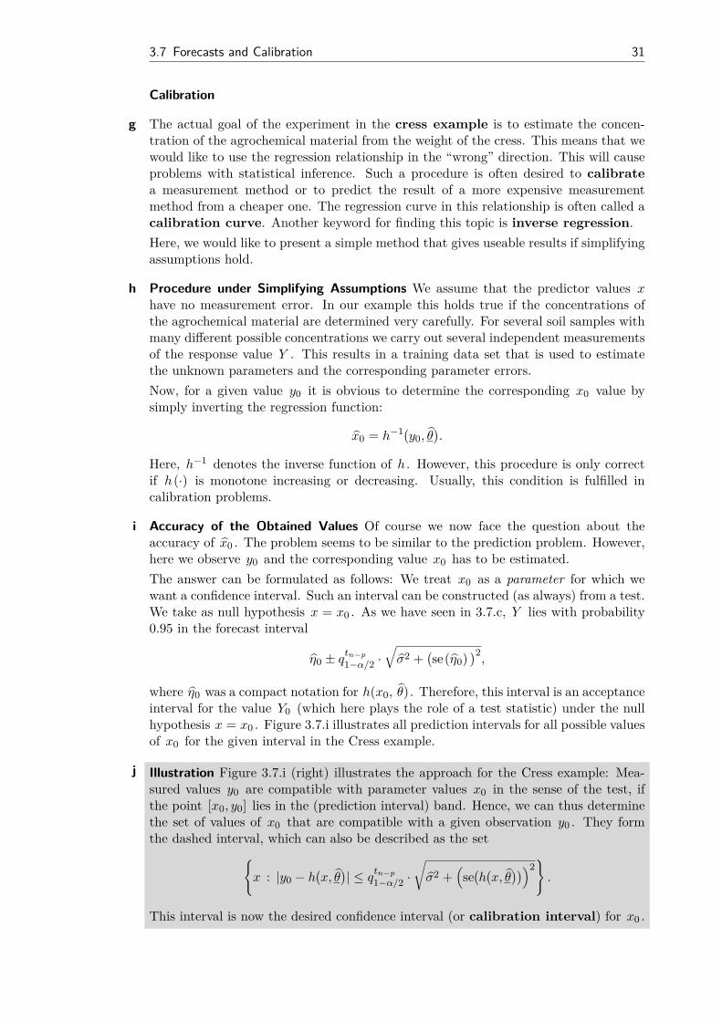
where η0 was a compact notation for h(x0, θ). Therefore, this interval is an acceptanceinterval for the value Y0 (which here plays the role of a test statistic) under the nullhypothesis x = x0 . Figure 3.7.i illustrates all prediction intervals for all possible valuesof x0 for the given interval in the Cress example.

j Illustration Figure 3.7.i (right) illustrates the approach for the Cress example: Mea-sured values y0 are compatible with parameter values x0 in the sense of the test, ifthe point [x0, y0] lies in the (prediction interval) band. Hence, we can thus determinethe set of values of x0 that are compatible with a given observation y0 . They formthe dashed interval, which can also be described as the set{

x : |y0 − h(x, θ

)| ≤ qtn−p

1−α/2 ·√σ2 +

(se(h(x, θ

)))2}.

This interval is now the desired confidence interval (or calibration interval) for x0 .


0 1 2 3 4 5

0

200

400

600

800

1000

Concentration

Wei

ght

0 1 2 3 4 5

0

200

400

600

800

1000

Concentration

Wei

ght

Figure 3.7.i: Cress example. Left: Confidence band for the estimated regression curve (dashed)and forecast band (solid). Right: Schematic representation of how a calibration interval isdetermined, at the points y0 = 650 and y0 = 350. The resulting intervals are [0.4, 1.22] and[1.73, 4.34], respectively.

If we have m values to determine y0 , we apply the above method to y0 =∑mj=0 y0j/m

and get {x : |y0 − h

(x, θ

)| ≤

√σ2 +

(se(h(x, θ

)))2· qtn−p

1−α/2

}.

k In this chapter, only one of many possibilities for determining a calibration intervalwas presented.

3.8 Closing Comments

a Reason for the Difficulty in the Biochemical Oxygen Demand Example Why didwe have so many problems with the Biochemical Oxygen Demand example? Let ushave a look at Figure 3.1.e and remind ourselves that the parameter θ1 represents theexpected oxygen demand for infinite incubation time, so it is clear that it is difficultto estimate θ1 , because the horizontal asymptote is badly determined by the givendata. If we had more observations with longer incubation times, we could avoid thedifficulties with the quality of the confidence intervals of θ .

Also in nonlinear models, a good (statistical) experimental design is essential. Theinformation content of the data is determined through the choice of the experimentalconditions and no (statistical) procedure can deliver information that is not containedin the data.

b Bootstrap For some time the bootstrap has also been used for determining confidence,prediction and calibration intervals. See, e.g. Huet, Bouvier, Gruet and Jolivet (1996)where also the case of non-constant variance (heteroscedastic models) is discussed. Itis also worth taking a look at the book of Carroll and Ruppert (1988).

3.8 Closing Comments 33

c Correlated Errors Here we always assumed that the errors Ei are independent. Like inlinear regression analysis, nonlinear regression models can also be extended to handlecorrelated errors and random effects.

d Statistics Programs Today most statistics packages contain a procedure that cancalculate asymptotic confidence intervals for the parameters. In principle it is thenpossible to calculate “t-profiles” and profile traces because they are also based on thefitting of nonlinear models (on a reduced set of parameters).

e Literature Notes This chapter is mainly based on the book of Bates and Watts (1988).A mathematical discussion about the statistical and numerical methods in nonlinearregression can be found in Seber and Wild (1989). The book of Ratkowsky (1989) con-tains many nonlinear functions h(·) that are primarily used in biological applications.

4 Analysis of Variance and Design ofExperiments

Preliminary Remark Analysis of variance (ANOVA) and design of experiments areboth topics that are usually covered in separate lectures of about 30 hours. Here, wecan only give a very brief overview. However, for many of you it may be worthwhileto study these topics in more detail later.Analysis of variance addresses models where the response variable Y is a function ofcategorical predictor variables (so called factors). We have already seen how suchpredictors can be applied in a linear regression model. This means that analysis ofvariance can be viewed as a special case of regression modeling. However, it is worth-while to study this special case separately. Analysis of variance and linear regressioncan be summarized under the term linear model.Regarding design of experiments we only cover one topic, the optimization of aresponse variable. If time permits, we will also discuss some more general aspects.

4.1 Multiple Groups, One-Way ANOVA

a We observe g groups of values

Yhi = µh + Ehi i = 1, 2, . . . , nh; h = 1, 2, . . . , g,

where Ehi ∼ N (0, σ2), independent.The question of interest is whether there is a difference between the µh ’s.

b Null hypothesis H0 : µ1 = µ2 = . . . = µg .

Alternative HA : µh 6= µk for at least one pair (h, k).

Test statisticBased on the average of each group Y h. = 1

nh

∑nhi=1 Yhi we get the “mean squared error

between the different groups”

MSG = 1g − 1

g∑h=1

nh(Y h. − Y ..)2.

This can be compared to the “mean squared error within the groups”

MSE = 1n− g

∑h,i

(Yhi − Y h.)2,

leading to the test statistics of the F-test:

T = MSG

MSE,

which follows an F -distribution with g− 1 and n− g degrees of freedom under H0 .

34

4.2 Random Effects, Ring Trials 35

Df Sum of Sq Mean Sq F Value Pr(F)

Treatment 4 520.69 130.173 1.508 0.208Error 77 6645.15 86.301

Total 81 7165.84

Table 4.1.b: Example of an ANOVA table.

Lab

Sr−

89

5 10 15 20

4050

6070

8090

57.7

Figure 4.2.a: Sr-89-values for the 24 laboratories

c Non-parametric tests (if errors are not normally distributed):“Kruskal-Wallis-Test”, based on the ranks of the data.For g = 2 groups: “Wilcoxon-Mann-Whitney-Test”, also called “U-Test”.

4.2 Random Effects, Ring Trials

Example a Strontium in Milk Figure 4.2.a illustrates the results of a ring trial (an inter-laboratorycomparison) to determine the concentration of the radioactive isotope Sr-89 in milk(the question was of great interest after the Chernobyl accident). In 24 laboratoriesin Germany two runs to determine this quantity in artificially contaminated milk wereperformed. For this special situation the “true value” is known: it is 57.7 Bq/l. Source:G. Haase, D. Tait und A. Wiechen: “Ergebnisse der Ringanalyse zur Sr-89/Sr-90-Bestimmung in Milch im Jahr 1991”. Kieler Milchwirtschaftliche Forschungsberichte43, 1991, S. 53-62).Figure 4.2.a shows that the two measurements of the same laboratory are in generalmuch more similar than measurements between different laboratories.

b Model: Yhi = µ+Ah + Ehi . Ah random, Ah ∼ N (0, σ2A).

Special quantities can tell us now how far two measurements can be from each othersuch that it is still safe to assume that the difference is only random.

• Comparisons within laboratory: “Repeatability” 2√

2 · σE ,• Comparisons between laboratories: “Comparability” 2

√2(σ2

E + σ2A)

36 4 Analysis of Variance and Design of Experiments

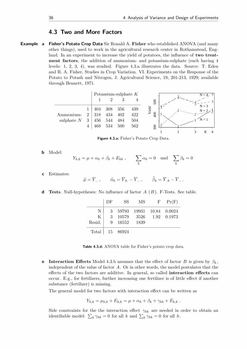
4.3 Two and More Factors

Example a Fisher’s Potato Crop Data Sir Ronald A. Fisher who established ANOVA (and manyother things), used to work in the agricultural research center in Rothamstead, Eng-land. In an experiment to increase the yield of potatoes, the influence of two treat-ment factors, the addition of ammonium- and potassium-sulphate (each having 4levels: 1, 2, 3, 4), was studied. Figure 4.3.a illustrates the data. Source: T. Edenand R. A. Fisher, Studies in Crop Variation. VI. Experiments on the Response of thePotato to Potash and Nitrogen, J. Agricultural Science, 19, 201-213, 1929; availablethrough Bennett, 1971.

Potassium-sulphate K1 2 3 4

1 404 308 356 439Ammonium- 2 318 434 402 422sulphate N 3 456 544 484 504

4 468 534 500 562

1

1

1

1

2

22

23

3

33

4

44

4

Yie

ld

300

400

500

1 2 3 4K

N = 1

N = 2N = 3

N = 4

Figure 4.3.a: Fisher’s Potato Crop Data.

b Model:Yh,k = µ+ αh + βk + Ehk ,

∑h

αh = 0 und∑k

βk = 0

c Estimates:µ = Y .. , αh = Y h. − Y .. , βk = Y .k − Y .. .

d Tests. Null-hypotheses: No influence of factor A (B ). F-Tests. See table.

DF SS MS F Pr(F)

N 3 59793 19931 10.84 0.0024K 3 10579 3526 1.92 0.1973

Resid. 9 16552 1839

Total 15 86924

Table 4.3.d: ANOVA table for Fisher’s potato crop data.

e Interaction Effects Model 4.3.b assumes that the effect of factor B is given by βk ,independent of the value of factor A . Or in other words, the model postulates that theeffects of the two factors are additive. In general, so called interaction effects canoccur. E.g., for fertilizers, further increasing one fertilizer is of little effect if anothersubstance (fertilizer) is missing.The general model for two factors with interaction effect can be written as

Yh,k = µh,k + Eh,k = µ+ αh + βk + γhk + Eh,k .

Side constraints for the the interaction effect γhk are needed in order to obtain anidentifiable model:

∑h γhk = 0 for all k and

∑k γhk = 0 for all h .

4.4 Response Surface Methods 37

However, parameters can only be estimated if there are two or more observations foreach combination of (h, k) (replicates).

f It’s not difficult to extend model 4.3.b for more than two factors. The generalmodel then also contains “interactions of higher order”.

g For product development it’s often necessary to check the effect of several (many)factors. In order to avoid too many experiments, it’s often useful to restrict eachfactor to two levels and to avoid replicates. Such a series of experiments for k factorsis called 2k -design and will be discussed in more detail in the next section.

4.4 Response Surface Methods

Example a Antibody Production Large amounts of antibodies are obtained in biotechnologicalprocesses: Host animals (e.g. mice) are injected with modified cells that can producethe corresponding antibody. After a certain time these cells start to produce antibodiesthat can be collected in excreted fluid for further processing.The cells can only produce antibodies if the immune system of the host animal isbeing weakened at the same time. This can be done with 4 factors. Moreover, it isbelieved that the amount of injected cells and their development stage has an influenceon antibody production.As there are no theoretical models for such complex biological processes, the relevantprocess factors have to be determined by an experiment. Such an experiment needsmany mice, is time-intensive and usually costs a lot of money. Using a clever design,we can find out the important process factors with the lowest possible effort. That’swhere statistical design of experiments comes into play.Two relevant process factors were identified in this study: the dose of Co60 gammarays and the number of days between radiation and the injection of a pure oil. Now,the question is to find the levels for these two factors such that an optimal amountof antibodies is being produced by the modified cells.

b We have already seen a model which models a response variable Y that depends ontwo factors. It was

Yh,k = µh,k + Eh,k = µ+ αh + βk + γhk + Eh,k , h, k = 1, 2.

If the two factors are based on continuous variables x(1), x(2) , as is the case here withradiation dose and the number of days between radiation and injection, we have thecorresponding general model

Yi = h(x

(1)i , x

(2)i

)+ Ei,

(analogous for more than two factors). The function h(x(1), x(2)

), which depends on

x(1) and x(2) , is the so-called response surface. Usually a quadratic polynomial(see below) in the variables x(1) and x(2) is used for h (sometimes the function h isavailable from theory). Once we have h , we can find the optimal setting [x(1)

0 , x(2)0 ] of

the process factors. Usually, h must be estimated from data.


•

•

•

•

•

80 90 100 110 120

40

50

60

70

80

Time [min]

Yie

ld [g

ram

s]

•

•

• •

•

180 200 220 240 260

40

50

60

70

80

Temperature [Celsius]

Yie

ld [g

ram

s]

Figure 4.4.c: Varying the variables one by one. Left: Yield vs. reaction time, reaction tem-perature held constant at 220◦C . Right: Yield vs. reaction temperature, reaction time heldconstant at 100 minutes.

c A naive approach to find the optimum would be to optimize the variables one by one.The weakness of such an approach is now being illustrated with an artificial example.

Example d Reaction Analysis A chemist wants to maximize the yield of a chemical reaction byvarying reaction time and reaction temperature. First, he performs an experimentwhere he uses a constant reaction temperature of T = 220◦C and reaction times 80,90, 100, 110, and 120 minutes. Results are illustrated in Figure 4.4.d. According tothis data, the maximum is attained with a reaction time of about 100 minutes.In a second stage, reaction time is held constant at its optimal value of t = 100 minutes.Reaction temperature is varied at 180, 200, 220, 240, and 260◦C . Now, the conclusionis that maximal yield is attained with a reaction temperature of about 220◦C . Thisis not too far away from the value that was used in the first stage. Hence, the finalconclusion is that the maximal yield of about 65 grams is attained using a reactiontime of about 100 minutes and a reaction temperature of about 220◦C .

e To see that this conclusion is wrong, we have to make use of a two-dimensional view.Let us put time on the x- and temperature on the y -axis. Yield is illustrated by thecorresponding contours (Figure 4.4.e). In this example, maximal yield of about 70grams is attained with a reaction time of about 85 minutes and a reaction temperatureof about 270◦C .The approach of “varying the variables one by one” is misleading because it tacitlyassumes that the maximal value of one variable is independent of the other ones. Thisassumption is usually not fulfilled.

f Even though the original setting of the process variables was “far away” from theoptimal value, an appropriate sequence of well chosen experimental set-ups leads tothe optimum. For that purpose, we start with a so called first-order design, a2k -design with additional measurements in the center. Experience from earlier exper-iments should guide us in selecting appropriate levels for the factors.

Example g Reaction Analysis (cont’d) From earlier experiments we know that a reaction tem-perature of 140◦C and a reaction time of 60 minutes gives good results. Now we wantto vary reaction time by 10 minutes and reaction temperature by 20◦C . The corre-


70 80 90 100 110 120

180

200

220

240

260

280

300

50

50

606568

• • • • •

•

•

•

•

•

Time [min]

Tem

pera

ture

[Cel

sius

]

Figure 4.4.e: A hypothetical response surface, illustrated by contours in the diagram reactiontemperature vs. reaction time.

sponding first-order design and the corresponding measurement results can be foundin Table 4.4.g. Usually, coded variables are used in literature. They can also be foundin Table 4.4.g.

Variable Variable Yieldin original units in coded units

Run Temperature [◦C] Time [min] Temperature Time Y [grams]

1 120 50 –1 –1 522 160 50 +1 –1 623 120 70 –1 +1 604 160 70 +1 +1 705 140 60 0 0 636 140 60 0 0 65

Table 4.4.g: First-order design and measurement results for the example “Reaction Analysis”.The single experiments (runs) were performed in random order : 5, 4, 2, 6, 1, 7, 3.

h Because the response surface h (see 4.4.b) is unknown, we approximate it with thesimplest possible surface, a plane. Hence, we have the model

Yi = θ0 + θ1x(1)i + θ2x

(2)i + Ei,

which has to be fitted to the data. We have already seen how the parameter estimatescan be obtained.The fitted plane, the so called first-order response surface, is given by

y = θ0 + θ1x(1) + θ2x

(2).

Of course, this is only an approximation of the real response surface.


Estimate Std. Error t value Pr(> |t|)(Intercept) 62.000 0.882 70.30 6.3e-06 ***xt1 5.000 1.080 4.63 0.019 *xt2 4.000 1.080 3.70 0.034 *

Table 4.4.i: Estimated coefficients for the coded variables in the example “Reaction Analysis”.

Example i Reaction Analysis (cont’d) The parameters with respect to the coded variables canbe found in Table 4.4.i.

j On the first-order response surface we can find those points [x(1), x(2)]T which have aconstant yield y = y0 . From equation

y0 = θ0 + θ1x(1) + θ2x

(2)

we find the straight line

x(2) = y0 − θ0 − θ1x(1)

θ2

with slope b = −θ1/θ2 and intercept a = (y0− θ0)/θ2 . Orthogonal to this straight lineis the direction of steepest ascent (descent). This straight line has slope θ2/θ1 .The two-dimensional vector [θ1, θ2]T is called estimated gradient; this direction is thefastest way to get large values of y .Of course we also get large values when following any direction that is “close” to thegradient.

k Observations that are in the center of the 2k -design have no influence on the estimatesof the parameters θ1, . . . , θk and hence no influence on the estimated gradient, either.This can be seen from the normal equations.But why should we do experiments in the center?• It’s possible to estimate the measurement error without using the assumption

that the plane is a good approximation of the true response surface if severalobservations are available in the center.

• Possible curvature of the true response surface can be detected. If there is nocurvature and if the plane is a “good” approximation of the true response sur-face in the range of the experimental set-up, the average of the observations inthe center, Y c , and the average of the observations of the 2k -design, Y f , areestimates of the mean of Y for the set-up in the center. Hence, they should be“more or less equal”. If the difference is obviously different from zero it’s a hintthat there is curvature.

A statistical test for curvature is as follows: The empirical variance s2 that was esti-mated from the nc observations in the center can be used to determine the standarddeviation of the difference. The variance of Y c can be estimated by s2/nc and thevariance of Y f by s2/2k . Because Y c and Y f are independent, the variance of thedifference Y c − Y f is estimated by s2(1/nc + 1/2k). Now we can perform a t-test orwe can construct the corresponding confidence interval: If the interval

Y c − Y f ± qtnc−10.975 ·

√s2(1/nc + 1/2k)

does not cover zero, the difference is statistically different from zero.


If we face relevant curvature of the true response surface (in the range of the exper-imental set-up), a linear approximation is not appropriate. Hence, we may also haveproblems determining the direction of steepest ascent. Usually we will use a second-order response surface (see below) for such situations.

l If the measurements of the center observations are all performed in a row, we facethe danger that the observed variation (measured by s2 ) is not really the variationbetween “independent” observations. Usually we will get significant curvature, evenfor cases where the response surface is a plane.In general, it’s important to randomize the different experimental set-ups –even though this usually needs much more effort because we always have to arrange anew setting for each new run.

m If it’s plausible to use a linear response surface, we will search for an optimum alongthe direction of steepest ascent. Along[

x(1)0x

(2)0

]+ k

[c(1)

c(2)

]

we will perform additional experiments for k = 1, 2, . . . until yield starts to decrease.[x(1)

0 , x(2)0 ]T is the point in the center of our experimental design and [c(1), c(2)]T is

the direction of steepest ascent.

Example n Reaction Analysis (cont’d) The first-order response surface is

y = 62 + 5x(1) + 4x(2) = 3 + 0.25 · x(1) + 0.4 · x(2),

where [x(1), x(2)]T are the coded x-values (taking values ±1) (see Table 4.4.i). Notethat the gradient for the coded and the non-coded (original) x-values lead to differentdirections of steepest ascent. An other ascent direction can be identified by observingthat individually increasing temperature by 4◦C or time by 2.5 minutes both leads toa yield increase of 1 gram.Further experiments are now performed along[

14060

]+ k ·

[2510

],

which corresponds to the steepest ascent direction with respect to the coded x-values,(see Table 4.4.n).

Temperature [◦C] Time [min] Y

1 165 70 722 190 80 773 215 90 794 240 100 765 265 110 70

Table 4.4.n: Experimental design and measurement results for experiments along the steepestascent direction for the example “Reaction Analysis”.


Based on the results in Table 4.4.n (plot the profile of yield vs. runs), the optimumshould be in the neighborhood of a reaction temperature of 215◦C and a reaction timeof 90 minutes.

o Once the optimum along the gradient is identified, a further first-order design ex-periment can be performed (around the optimum) to get a new gradient. However,in general the hope is that we are already close to the optimal solution and we willcontinue as illustrated in the next section.

4.5 Second-Order Response Surfaces

a Once we are close to the optimal solution, the estimated plane will be nearly parallelto the (x(1), x(2))-plane. Hence, θ1 and θ2 will be nearly zero. We expect that theoptimal solution is a (flat) peak in the range of our experimental set-up and hence weexpect the difference Y c − Y f to be significantly different from zero. Such a peak canbe modelled by a second-order polynomial:

Yi = θ0 + θ1x(1)i + θ2x

(2)i + θ11(x(1)

i )2 + θ22(x(2)i )2 + θ12x

(1)i x

(2)i + Ei

b However, the 2k -design does not contain enough data to estimate the parameters ofthe second-order polynomial. The reason is that we need at least 3 levels for eachfactor. There are now several ways of expanding our original design. The more levelswe have for each factor, the better we can estimate the curvature. So called rotatablecentral composite designs (also called second-order central composite designs) arevery famous. As can be seen from the graphical representation in Figure 4.5.b wecan get such a design by extending our original first-order design. In total we have 9different experimental set-ups if we have two predictor variables. All points (exceptthe center point) have the same distance from the center (0, 0). Five levels areused for each factor. If we use replicates at (0, 0) we get a more precise estimate ofthe quadratic part of the model.

Example c Reaction Analysis (cont’d) A rotatable central composite design was applied. Theresults can be found in Table 4.5.c.The parameter estimates lead to the estimated second-order response surface:

y = θ0 + θ1x(1) + θ2x

(2) + θ11(x(1))2 + θ22(x(2))2 + θ12x(1) x(2)

= −278 + 2.0 · x(1) + 3.2 · x(2) + 0.0060 · (x(1))2 + 0.026 · (x(2))2 + 0.006 · x(1) x(2).

d Depending on the parameters, a second-order response surface can take differentshapes. The most important ones are those that have a maximum (minimum) ora saddle (rather rare). A schematic contour plot of these two types is illustrated inFigure 4.5.d.

Surfaces with a maximum (minimum) don’t need further explanations: Once we leavethe optimum in any direction, yield Y is decreasing (increasing). For a saddle, itdepends on the direction whether yield Y increases or decreases. Hence, the surfaceis like a horse saddle.

4.5 Second-Order Response Surfaces 43

-1 0 1

-1

0

1

Figure 4.5.b: Rotatable central composite design. It consists of a 22 -design (v) with additionalexperiments in the center and along the axes (p).

Variables Variables Yieldin original units in coded units

Run Temperature [◦C] Time [min] Temperature Time Y [grams]

1 195 80 −1 −1 782 235 80 +1 −1 763 195 100 −1 +1 724 235 100 +1 +1 755 187 90 −

√2 0 74

6 243 90 +√

2 0 767 215 76 0 −

√2 77

8 215 104 0 +√

2 729 215 90 0 0 80

Table 4.5.c: Rotatable central composite design and measurement results for the example “Re-action Analysis”.

e It’s possible to find an analytical solution for the critical point by calculating partialderivatives. In the critical point they have to be zero:

∂Y

∂x(1) = θ1 + 2 θ11 x(1)0 + θ12 x

(2)0 = 0

∂Y

∂x(2) = θ2 + 2 θ22 x(2)0 + θ12 x

(1)0 = 0 .

Solving this linear equation system for x(1)0 and x

(2)0 leads us to

x(1)0 = θ12 θ2 − 2 θ22 θ1

4 θ11 θ22 − θ212

x(2)0 = θ12 θ1 − 2 θ11 θ2

4 θ11 θ22 − θ212

.


x(1)

x(2) 10

9

8

7

x(1)

x(2) 10

1112

13

98

7

Figure 4.5.d: Contour plots of second-order response surfaces with a maximum (left) and asaddle (right).

Example f Reaction Analysis (cont’d) We can directly read the critical values off the contourplot in Figure 4.5.f: (220◦C , 85 minutes).

150 200 250

50

60

70

80

90

100

110

707578

80

• •

• ••

Temperature [Celsius]

Tim

e [m

in]

Figure 4.5.f: Estimated response surface and experimental designs for the example “ReactionAnalysis”. The first-order design is marked with u, the experiments along the steepest ascentwith vand those of the rotatable central composite design with �E.

Example g Antibody production (cont’d) Let’s come back to our original example. A radioactivedose of 200 rads and a time of 14 days is used as starting point. Around this point weuse a first-order design, see Table 4.5.g.Based on the measurements in the center we can calculate the standard deviation ofthe error term: σ = 53.9. Now we check whether there is significant curvature. Theconfidence interval for the difference can be calculated as outlined in 4.4.k:

Y c − Y f ± qtnc−10.975 ·

√s2(1/nc + 1/2k) = 589− 335± 4.30 · 41.1

= [77, 431].

As this interval does not cover 0, the difference is statistically different from zero on the

4.5 Second-Order Response Surfaces 45


Run RadDos [rads] Time [days] RadDos Time Y

1 100 7 −1 −1 2072 100 21 −1 +1 2573 300 7 +1 −1 3064 300 21 +1 +1 5705 200 14 0 0 6306 200 14 0 0 5287 200 14 0 0 609

Table 4.5.g: First-order design and measurement results for the example “AntibodyProduction”.

5% level. As yield decreases at the border of our experimental set-up, we conjecturethat the optimal value must lie somewhere within our set-up range.Hence, we expand our design to a rotatable central composite design by doing addi-tional measurements (see Table 4.5.g).


Run RadDos [rads] Time [days] RadDos Time Y

8 200 4 0 −√

2 3159 200 24 0 +

√2 154

10 59 14 −√

2 0 10011 341 14 +

√2 0 513

Table 4.5.g: Rotatable central composite design and measurement results for the example “An-tibody Production”.

The estimated response surface is

Y = −608.4 + 5.237 · RadDos + 77.0 · Time−0.0127 · RadDos2 − 3.243 · Time2 + 0.0764 · RadDos · Time.

We can identify the optimal conditions in the contour plot (Figure 4.5.g):RadDosopt ≈ 250 rads and timeopt ≈ 15 days.

h Summary To find the optimal setting of our variables (leading to maximal yield) wehave to iteratively do experiments using special designs.• If we are still “far away” from the optimum, we use first-order designs and we

estimate the corresponding first-order response surface (a plane).• On the estimated response surface we determine an ascent direction. Along that

direction we do additional experiments until the response variable decreases again(“extrapolation”).

• Further first-order experiments may be performed (hence we repeat the last twosteps).

• As soon as we are close to the optimum, we perform (e.g.) a rotatable centralcomposite design (or we expand our first-order design) to estimate the second-


50 100 150 200 250 300 350

5

10

15

20

25

300 300

400

500550590

610

RadDos [rads]

Tim

e [d

ays]

Figure 4.5.g: Estimated second-order response surface for the example “antibody production”.

order response surface. The optimum on that response surface can be determinedeither analytically or graphically.

4.6 Experimental Designs, Robust Designs

a Here we discussed two types of experimental designs in more detail. Of course thereare books full of other designs that are useful for various scopes. The subject is calleddesign of experiments.It may be worthwhile to note that for situations where little is known about theinfluence of the predictors on the response, so called “screening designs” can bevery useful. They allow a (rough) analysis of k factors with less than 2k experiments.

b The idea of “robust product design” is that products should have constant qualityeven if production conditions vary. To reach this goal we do not only have to optimizethe expected quality (or yield or other response variables) but also the variability.There are special designs for that purpose, e.g. the Taguchi designs.

4.7 Further Reading

• ANOVA and Design of Experiments Short overviews of simple ANOVAmodels can be found in Hartung, Elpelt and Klosener (2002, Chap. XI) and Sachs(2004, Chap. 7). Linder and Berchtold (1982) give a more detailed introduction.

• Applied books about ANOVA and design of experiments are the famous book ofBox, Hunter and Hunter (1978) and the book of Daniel (1976).

• A special book that uses unusual ways to introduce known (and unknown) meth-ods with focus an explorative analysis is Hoaglin, Mosteller and Tukey (1991).

• A classical mathematically oriented book about ANOVA is Scheffe (1959).• Design of Experiments Federer (1972, 1991) is an introduction to statistics

4.7 Further Reading 47

where design of experiments often takes center stage. More details can be foundin the already mentioned book of Box et al. (1978) but also in Mead (1988).

• A systematic overview of experimental design can be found in Petersen (1985).• A few books discuss topics about practical application of statistics that can’t

be dealt with mathematics. Recommendations are Boen and Zahn (1982) andChatfield (1996).

• Response Surfaces An introduction to response surfaces is available in Box etal. (1978, Chapter 15) or in Hogg and Ledolter (1992).Box and Draper (1987) and Myers and Montgomery (1995) cover more details.

5 Multivariate Analysis of Spectra

5.1 Introduction

a “Spectrum” means here: We measure the “intensity” for certain “wave lengths”. Sucha function characterizes a chemical mixture (or as a special case a pure substance).There are many spectra in chemistry. For some of them, pure substances have aspectrum that consists of a single “peak”. As long as the peaks are not overlapping,we can identify the different components of a mixture and their proportions.

b NIR-Spectra (near infrared): The NIR-Spectra of pure substances is “any” functionwith some more or less characteristic peaks. Hence, it’s rather difficult to identify thetype and the quantity of the different components based on the spectrum of a chemicalmixture. On the other side, these spectra are very cheap: No extra processing is needed,they can be measured on-line.

Example c Quality Control via NIR-Spectra We have data of reflections of NIR-waves on 52granulate samples with wave length 1100, 1102, 1104, ..., 2500 nm. Figure 5.1.c showsthe spectra in “centered” form; for each wave length j the median value medi(X(j)

i )was subtracted from the X(j)

i ’s.

Wl. 1800 1810 ... 2500a 0.003097 0.017238 ... −0.02950b 0.002797 0.016994 −0.03095c 0.002212 0.015757 −0.03095

...Z 0.001165 0.014237 ... −0.03110

Table 5.1.c: Data for the example “NIR-spectra” (for wavelengths larger than 1800nm).

Questions• There are outliers. Are there other “structures”?• The amount of an active ingredient was determined with a chemical analysis.

Can we estimate it sufficiently accurate with the spectrum?

d In other applications we measure spectra to follow a reaction on-line. It is used for• estimating the order of a reaction and to determine potential intermediate prod-

ucts and reaction constants,• determining the end of a process,• monitoring a process.

We can also automatically monitor slow processes of all kinds. For example stock-keeping: Are there any (unwanted) aging effects?

48

5.2 Multivariate Statistics: Basics 49

1100 1300 1500 1700 1900 2100 2300 2500

−0.

006

0.00

00.

006

0.01

20.

018

Wave length

Spe

ctru

m, m

ed−

cent

ered

Figure 5.1.c: NIR-Spectra of granulate samples, centered at the median curve.

e For each observation (sample) we have many variables (a whole spectrum).Questions• Is it reasonable to plot the different samples on a plane or is it possible to catch

most information and see structure from just a few dimensions (instead of usingall variables)?

• Can we identify dimensions (with technical interpretation) in the high-dimensionalspace that contain most of the information?

• Is it possible to identify and to quantify the different components of a chemicalmixture based on its spectrum?

• For a regression analysis, 70 variables (or 700 at a higher resolution) are toomuch if we only have 52 observations. How should we reduce dimensionality?

5.2 Multivariate Statistics: Basics

a Notation The vector Xi = [X(1)i , X

(2)i , ..., X

(m)i ]T denotes the ith spectrum. It’s a

point in m-dimensional space. Hence, for each observation we measure m differentquantities.Remark In statistics and probability theory vectors are usually column vectors. Rowvectors are denoted by the symbol T (transposed vector).This is inconvenient in statistics because the data matrix

X = [X(j)i ] ,

that consists of n observations of m variables is built up the other way round: Theith row contains the values for the ith observation. For most applications this is auseful table (see e.g. the design matrix of a linear regression model). Here, it’s oftenthe other way round: In a table of spectra, a column often contains a single spectrum(i.e., it’s one observation of a spectrum).

50 5 Multivariate Analysis of Spectra

b Definitions We define the following quantities for an m-dimensional random vectorX = [X(1), X(2), ..., X(m)]T ∈ Rm .• Expectation µ ∈ Rm

µ = (µ1, . . . , µm)T , where µk = E[X(k)], k = 1, . . . ,m .In other words: a vector that consists of the (univariate) expectations.We write µX in situations where we also have other random variables.

• Covariance Matrix |Σ ∈ Rm×m|Σ is an m×m matrix with elements

|Σjk = Cov(X(j), X(k)) = E[(X(j) − µj)(X(k) − µk)

].

We also use the notation Var(X) or Cov(X).Note that◦ |Σjj = Cov(X(j), X(j)) = Var(X(j)).

This means that the diagonal elements of the matrix are the variances.

◦ Corr(X(j), X(k)) = |Σ jk√|Σ jj |Σkk

.

Again, sometimes we write |ΣX if we want to point out that this is the covariancematrix that corresponds to X .

c Linear Transformations• For a simple (one-dimensional) random variable: Y = a+ bX, where a, b ∈ R .

Expectation: E[Y ] = a+ bµX .Variance: Var(Y ) = b2σ2

X .• For random vectors: Y = a+ BX, where a ∈ Rm, b ∈ Rm×m .

Expectation: E[Y ] = a+ BµX .Covariance: Cov(Y ) = B |ΣXB T .

d Remark The multivariate normal distribution X ∼ N (µ, |Σ) is fully characterizedby the mean µ and the covariance matrix |Σ . It is the most common distribution inmultivariate statistics. See e.g. Chapter 15.3 in Stahel (2000).Figure 5.2.d illustrates two two-dimensional normal distributions with the “contours”of their densities. The mean vector is responsible for the location of the distributionand the covariance matrix for the shape of the contours.

e Estimators

µ =[X

(1), X

(2), . . . , X

(m)]T = vector of means

|Σ = 1n− 1

n∑i=1

(Xi − µ)(Xi − µ)T

= matrix of the empirical variances and covariances.

This means that

|Σjk = 1n− 1

n∑i=1

(X(j)i −X

(j))(X(k)i −X

(k)).

The covariance matrix plays a crucial role in multivariate models that are based onthe normal distribution or that want to model linear relationships.

5.3 Principal Component Analysis (PCA) 51

−2 0 2

−2

02

0.65 0.70 0.75

0.4

0.5

0.6

z(1)

z(2)

x(1)

x(2)

Figure 5.2.d: Contours of the probability densities for a standard normal (left) and a general(right) multivariate normal distribution.

5.3 Principal Component Analysis (PCA)

a Our goal is dimensionality reduction. We are looking for a few dimensions in them-dimensional space that can explain “most of the variation in the data”.We define variation in the data as the sum of the individual m variances

m∑j=1

Var(X(j)) = 1n− 1

n∑i=1

m∑j=1

(X(j)i )2,

where X(j)i are the centered observations: X(j)

i = X(j)i −X

(j) .

We want to find a new “coordinate system” with certain properties. This will lead to• new basis vectors bk (‖bk‖ = 1), the so called principal components. The

individual components of these basis vectors are called loadings.• new coordinates Z(k)

i = XTi bk , the so called scores (projections of the data on

the directions above).

What properties should the new coordinate system have?• The first basis vector b1 should be chosen such that Var(Z(1)) is maximal.• The second basis vector b2 should be orthogonal to the first one (bT2 b1 = 0) such

that Var(Z(2)) is maximized.• And so on...

Figure 5.3.a illustrates the idea using a two-dimensional distribution.To summarize, we are performing a transformation to new variables

Zi = BT (Xi − µ),

where the transformation matrix B is orthogonal.It can be shown that B is the matrix of (standardized) eigenvectors and λk are theeigenvalues of |ΣX .Remember that |ΣX is a symmetric matrix and therefore we can decompose it into

|ΣX = B D BT,


where B is the matrix with the eigenvectors in the different columns and D is thediagonal matrix with the eigenvalues on the diagonal (this is a fact from linear algebra).Therefore we have

Var(Z) = BT |ΣXB = D =

λ1 0 . . . 00 λ2 . . . 0...

... . . .0 0 . . . λm

λ1 ≥ λ2 ≥ · · · ≥ λm ≥ 0.

Hence, the individual components of Z are uncorrelated and the first componentof Z has largest variance. By construction it holds that λ1 = Var(Z(1)). It is themaximal variance of a projection:

λ1 = maxb:‖b‖=1

(Var(X b)).

Accordingly for λm : It’s the smallest variance.Because the λk are the eigenvalues of |ΣX , we know from linear algebra that

m∑k=1

λk =m∑k=1

|Σkk =m∑k=1

Var(X(j)).

Hence ∑kj=1 λj∑mj=1 λj

is the proportion of the total variance that is explained by the first k principalcomponents.Of course we can always go back to the original data using the new variables by doinga simple back-transformation

Xi − µ =(

BT)−1

Zi = BZi =m∑k=1

Z(k)i b(k).

b Graphical Representation By reducing dimensionality it gets easier to visualizethe data. For that reason we only consider the first two (or three) components andforget about the other ones. Figure 5.3.b (i) illustrates the first two components forthe “NIR-spectra” example (for technical reasons we only consider wave lengths largerthan 1800 nm). We can see 5 outliers – they were already visible in the spectra. Figure5.3.b (ii) shows the first three components of a principal component analysis withoutthe outliers.


log

(w

idth

)

0.65 0.75

0.5

0.6

10

1. Principal Component

2. P

rinci

pal C

ompo

nent

−0.1 0 0.1

−0.

10

0.1

Figure 5.3.a: Principal component rotation.

ab

c

d

e

f

gh

i

j

k

l

m

n

o

p

q

rs

t

uv

w

x

y

zA

B

C

D

E

F

G

H

I

J

KL M

N O P

Q

RS

T

U

V

W

X

YZ

−0.015 −0.005 0.005 0.015 0.025 0.035

−0.

014

−0.

008

−0.

002

0.00

40.

010

Comp. 1

Com

p. 2

Figure 5.3.b: (i) Scatterplot of the first two principal components for the example “NIR-spectra”.


Comp.1

−0.016 −0.006 0.004

ab

c

d

e

f

gh

i

j

k lm

n

o

p

q

rs

t

uvw

x

y

z A B

C

D

EF

GH

I

JKLM

NO

RST

VY Z

−0.

014

−0.

004

0.00

60.

014

a b

c

d

e

f

gh

i

j

k lm

n

o

p

q

rs

t

uv

w

x

y

zA B

C

D

EF

GH

I

JK

LMNO

RS

TVYZ

−0.

016

−0.

006

0.00

4

a

bc

de

f

ghi

jk

l

mn

o

p

q

rs

tuvw

x

yz

A

B

C

D

E

F

GH

I

J KLM

N

O

R

S TV

YZ

Comp.2 a

bc

de

f

g hi

jk

l

mn

o

p

q

rs

t uvw

x

yzA

B

C

D

E

F

GH

I

JK LMN

O

R

S TV

YZ

−0.014 −0.004 0.006 0.014

a

bc

de f

g

hi

jklm n

op

q

rs

t

uvwx y

zA

B

CD

EF G

HIJ

KLMNO

RS

T VY

Z

a

bc

def

g

hi

jk lmn

op

q

rs

t

uvwx y

z A

B

CD

EF G

HIJ

KLMNO

RSTV

Y

Z

−0.0045 −0.0020 0.0005 −0.

0045

−0.

0020

0.00

05

Comp.3

Figure 5.3.b: (ii) Scatterplot matrix of the first three principal components for the example“NIR-spectra” without the 5 outliers.

c PCA is suitable for many multivariate data sets. If we are analyzing spectra we havethe special case that the variables (the intensities of different wavelengths) have aspecial ordering. Hence, we can plot each observation as a “function”. We can alsoillustrate the principal component directions (the loadings) bk as spectra!

d Scaling Issues If the variables are measured in different units, they should be stan-dardized to (empirical) variance 1 (otherwise comparing variances doesn’t make sense).This leads to a PCA (= eigenanalysis) of the correlation- instead of the covariance ma-trix.For spectra this is not useful because wavelengths with very variable intensities containthe most important information. If we would standardize the variables in that setup,we would down-weight these variables compared to the unstandardized data set.

e Choosing the number p of components: (p < m)• 2 (maybe 3) for illustrational purposes.• Plot the explained variance (eigenvalues) in decreasing order and look for a break-

point (“scree plot”: plot λk vs. k ), see Figure 5.3.e.• “Explain 95% of the variance”: The sum of the eigenvalues

∑pj=1 λj should be

95% of the total sum∑mj=1 λj .


1800 1900 2000 2100 2200 2300 2400 2500

−0.

20−

0.10

0.00

0.10

0.20

Wave length

Spe

ctru

m

Comp. 1Comp. 2Comp. 3

Figure 5.3.c: Spectra of “loadings” of the first three principal components for the example “NIR-spectra”.

Comp.1 Comp.3 Comp.5 Comp.7 Comp.9

NIR−spectra without 5 outliers

Var

ianc

es0.

0e+

002.

0e−

054.

0e−

05 Variances of princ. components

Figure 5.3.e: Variances of the principal components (scree plot) for the example “NIR-spectra”.

But: “Variance”∑mj=1 λj =

∑mj=1 Var(X(j)) is the sum of all variances. There could

be (many) noise variables among them!Restriction to the first p principal components: In the transformation formula (5.3.a)we simply ignore the last m− p terms:

Xi − µ = Xi + Ei , Xi =p∑

k=1Z

(k)i b(k) , Ei =

m∑k=p+1

Z(k)i b(k).

This can be interpreted in the following two ways.• In Linear Algebra terminology:

The “data matrix” of the Xi is the best approximation of the data matrix ofthe Xi − µ if we restrict ourselves to matrices with rank p (in the sense of theso-called Frobenius norm of matrices: ‖E‖2 =

∑ij E

2ij ).

• In statistical terminology:We were looking for p variables Z(k) =

∑mj=1BkjX

(j), k = 1, . . . p , such that thedifferences Ei = Xi − Xi of Xi =

∑pk=1 Z

(k)i b(k) show minimial variance (in the

sum):∑mj=1 Var(E(j)) =

∑mk=p+1 λk is minimal (there will be no better choice

than the variables Z(k) ).


5.4 Linear Mixing Models, Factor Analysis

a Model for Spectra Let ck be the spectrum of the chemical component k and considera mixture of the components with coefficients s = [s(k)] . For the ith mixture we havethe coefficients si . According to Lambert-Beer the spectrum of the ith mixture is

Xi =∑k

c(k)s(k)i + Ei = C si + Ei

where Ei are measurement errors. C is the matrix of spectra ck (in the differentcolumns).This looks very similar to 5.3.e. The differences are• C not orthogonal• Xi instead of Xi − µ , not centered• Ei random vector (measurement error)• s

(k)i ≥ 0 or Cjk ≥ 0, X(j)

i ≥ 0 if we use the original spectra.

b This model can be used for many applications where there are m measurements thatare linear superimpositions of p < m components.Examples are:• Chemical elements in rocks that consist of several bed-rocks.• Trace elements in spring water that ran through different soil layers.

c If the source profiles (spectra) ck are known, the “contributions” s(k)i can be estimated

for each observation i separately using linear regression.However, it’s more interesting if both the source profiles and their contributions haveto be estimated from data. This can be achieved using a combination of statisticalmethods, professional expertise and application specific properties.

5.5 Regression with Many Predictors

a In the introductory example about NIR-spectra we discussed the question whether wecan “predict” the amount of an active ingredient based on a spectrum.Hence, we have a response variable Y and several predictors [x(1), ..., x(m)] . If we setup a linear regression model we face the problem that there are many more predictorsthan observations. Hence, it’s not possible to fit a “full model” (it would lead to aperfect fit).A possible remedy is to use “stepwise” regression: We start with just one predictorand add the most significant predictor in the next step (until some stopping criterionis met).Example: Granulate Samples.Y = yield. n = 44 (without “outliers”). Table 5.5.a shows a computer output. Forcomparison: Simple correlation between L2450 and yield: r = −0.57, R2 = 0.32.

b Better known are the following methods to handle the problem of having too manypredictors

1. Principal Component-Regression,2. Ridge Regression3. New methods like Lasso, Elastic Net, ...

5.5 Regression with Many Predictors 57

Value Std. Error t value Pr(>|t|) Signif(Intercept) 75.30372 0.07175 1049.52 0.000 ***L2450 -395.43390 76.70623 -5.16 0.000 ***L2010 -465.28939 142.44458 -3.27 0.002 **L1990 585.20468 128.49676 4.55 0.000 ***L2360 875.33702 160.04160 5.47 0.000 ***L2400 532.91971 117.74430 4.53 0.000 ***L2480 -301.44225 77.70208 -3.88 0.000 ***L2130 -501.39852 88.17596 -5.69 0.000 ***

Residual standard error: 0.2268 on 36 degrees of freedomMultiple R-Squared: 0.7212

Table 5.5.a: Computer output for a regression model after variable selection with stepwiseforward.

c Principal Component-Regression PCA of the predictors leads to new variables[Z(1), . . . , Z(p)] . The principal components are usually selected without examining therelationship with the response Y .Variant of Brown Brown (1993): Select them according to simple correlation with Y !

d Ridge Regression An easy way to ensure that the matrix X T X (that needs to beinvertible for least squares) is non-singular is to add a diagonal matrix λI , leading to

βλ = (X T X + λI )−1 X TY .

Bibliography

Bates, D. M. and Watts, D. G. (1988). Nonlinear regression analysis and its applica-tions, Wiley Series in Probability and Mathematical Statistics, Wiley, New York.

Bennett, J. H. (ed.) (1971). Collected Papers of R. A. Fischer; 1912-24, Vol. I, TheUniversity of Adelaide.

Boen, J. R. and Zahn, D. A. (1982). The Human Side of Statistical Consulting,Wadsworth Inc. Belmont.

Bortz, J. (2005). Statistik fur Sozialwissenschaftler, 6 edn, Springer, Berlin.Box, G. E. P. and Draper, N. R. (1987). Empirical Model-Building and Response

Surfaces, Wiley Series in Probability and Mathematical Statistics, Wiley, New York.Box, G. E. P., Hunter, W. G. and Hunter, J. S. (1978). Statistics for Experimenters,

Wiley, N. Y.Brown, P. J. (1993). Measurement, Regression, and Calibration, Clarendon Press,

Oxford, UK.Carroll, R. and Ruppert, D. (1988). Transformation and Weighting in Regression,

Wiley, New York.Chatfield, C. (1996). The Analysis of Time Series; An Introduction, Texts in Statistical

Science, 5 edn, Chapman and Hall, London, NY.Daniel, C. (1976). Applications of Statistics to Industrial Experimentation, Wiley Series

in Probability & Mathematical Statistics, Wiley, New York.Daniel, C. and Wood, F. S. (1980). Fitting Equations to Data, 2 edn, Wiley, N. Y. 1st

ed. 1971.Federer, W. T. (1972, 1991). Statistics and Society: Data Collection and Interpretation,

Statistics: Textbooks and Monographs, Vol.117, 2 edn, Marcel Dekker, N.Y.Harman, H. H. (1960, 1976). Modern Factor Analysis, 3 edn, University of Chicago

Press, Chicago.Hartung, J., Elpelt, B. and Klosener, K. (2002). Statistik. Lehr- und Handbuch der

angewandten Statistik, 13 edn, Oldenbourg, Munchen.Hoaglin, D. C., Mosteller, F. and Tukey, J. W. (1991). Fundamentals of Exploratory

Analysis of Variance, Wiley, N. Y.Hogg, R. V. and Ledolter, J. (1992). Applied Statistics for Engineers and Physical

Scientists, 2 edn, Maxwell Macmillan International Editions.Huet, S., Bouvier, A., Gruet, M.-A. and Jolivet, E. (1996). Statistical Tools for Non-

linear Regression: A Practical Guide with S-Plus Examples, Springer-Verlag, NewYork.

Lawley, D. N. and Maxwell, A. E. (1963, 1967). Factor Analysis as a Statistical Method,Butterworths Mathematical Texts, Butterworths, London.

Linder, A. and Berchtold, W. (1982). Statistische Methoden II: Varianzanalyse undRegressionsrechnung, Birkhauser, Basel.

Mead, R. (1988). The design of experiments, Cambridge University Press, Cambridge.

58

Bibliography 59

Myers, R. H. and Montgomery, D. C. (1995). Response Surface Methodology; Processand Product Optimization Using Designed Experiments, Wiley Series in Probabilityand Statistics, Wiley, NY.

Petersen, R. G. (1985). Design and Analysis of Experiments, Statistics Textbooks andMonographs, Marcel Dekker, N.Y.

Rapold-Nydegger, I. (1994). Untersuchungen zum Diffusionsverhalten von Anionen incarboxylierten Cellulosemembranen, PhD thesis, ETH Zurich.

Ratkowsky, D. A. (1989). Handbook of Nonlinear Regression Models, Marcel Dekker,New York.

Renner, R. M. (1993). The resolution of a compositional data set into mixtures of fixedsource compositions, Applied Statistics — Journal of the Royal Statistical Society C42: 615–631.

Sachs, L. (2004). Angewandte Statistik, 11 edn, Springer, Berlin.Scheffe, H. (1959). The Analysis of Variance, Wiley, N. Y.Seber, G. and Wild, C. (1989). Nonlinear regression, Wiley, New York.Stahel, W. A. (2000). Statistische Datenanalyse: Eine Einfuhrung fur Naturwis-

senschaftler, 3 edn, Vieweg, Wiesbaden.Swinbourne, E. S. (1971). Analysis of Kinetic Data, Nelson, London.

statistical and numerical methods for chemical...

Documents