statistical and machine learning techniques for...

José M. Gutiérrez, Summer School WP (Santiago, 2001) 2Jo

sé

Ma

nu

el

Gu

tié

rre

z, U

niv

ers

ida

d d

e C

an

tab

ria

.Jo

sé M

anu

el G

uti

érre

z, U

niv

ers

ida

d d

e C

an

tab

ria

. h

ttp

://p

erso

nal

es.u

nic

an.e

s/g

uti

erjm

Statistical and Machine LearningTechniques for

Weather Forecasting

Antonio S. Cofiño José M. GutiérrezDpto. de Matemática Aplicada,

Universidad de Cantabria, Santander

Miguel A. RodríguezInstituto de Física de Cantabria , CSIC/Universidad de Cantabria.

http://personales.unican.es/gutierjm

Rafael CanoFrancisco J. López

Instituto Nacional de Meteorología ,


sé

Ma

nu

el

Gu

tié

rre

z, U

niv

ers

ida

d d

e C

an

tab

ria

.Jo

sé M

anu

el G

uti

érre

z, U

niv

ers

ida

d d

e C

an

tab

ria

. h

ttp

://p

erso

nal

es.u

nic

an.e

s/g

uti

erjm

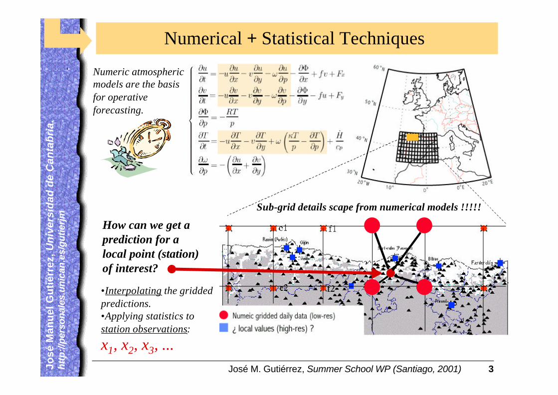
Numerical + Statistical Techniques

Sub-grid details scape from numerical models !!!!!

Numeric atmosphericmodels are the basisfor operative forecasting.

How can we get a prediction for a local point (station)of interest?

•Interpolating the gridded predictions.•Applying statistics to station observations:

x1, x2, x3, ...


sé

Ma

nu

el

Gu

tié

rre

z, U

niv

ers

ida

d d

e C

an

tab

ria

.Jo

sé M

anu

el G

uti

érre

z, U

niv

ers

ida

d d

e C

an

tab

ria

. h

ttp

://p

erso

nal

es.u

nic

an.e

s/g

uti

erjm

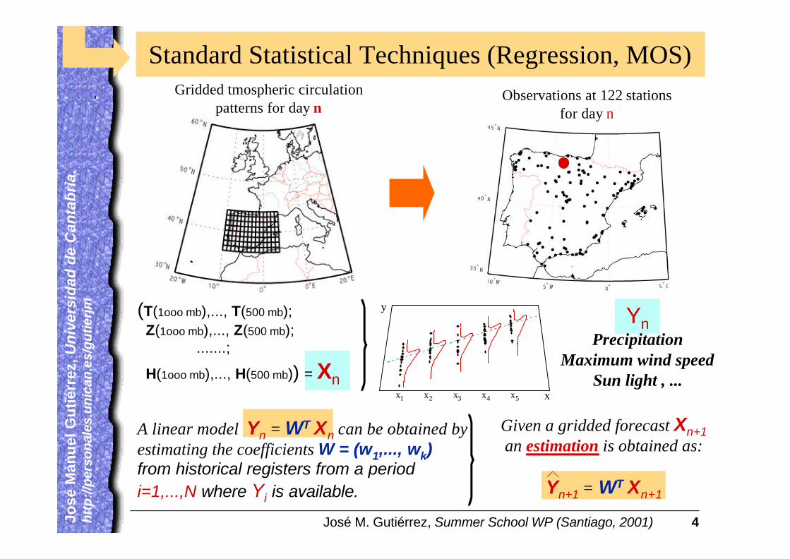
Standard Statistical Techniques (Regression, MOS)

YnPrecipitation

Maximum wind speedSun light , ...

(T(1ooo mb),..., T(500 mb); Z(1ooo mb),..., Z(500 mb);

.......;

H(1ooo mb),..., H(500 mb)) = Xn

Gridded tmospheric circulation patterns for day n

Observations at 122 stations for day n

Given a gridded forecast Xn+1an estimation is obtained as:

Yn+1 = WT Xn+1

A linear model Yn = WT Xn can be obtained by estimating the coefficients W = (w1,..., wk) from historical registers from a period i=1,...,N where Yi is available.

x

y

x1 x2 x3 x4 x5


sé

Ma

nu

el

Gu

tié

rre

z, U

niv

ers

ida

d d

e C

an

tab

ria

.Jo

sé M

anu

el G

uti

érre

z, U

niv

ers

ida

d d

e C

an

tab

ria

. h

ttp

://p

erso

nal

es.u

nic

an.e

s/g

uti

erjm

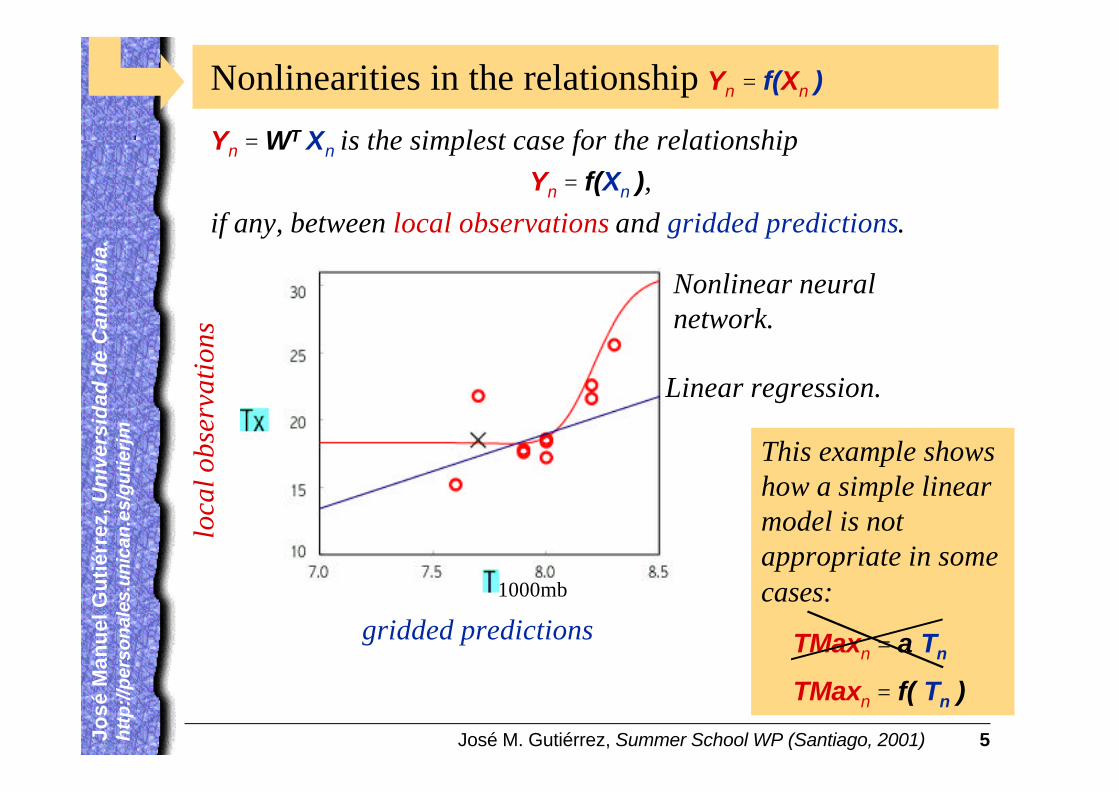
Nonlinearities in the relationship Yn = f(Xn )

Yn = WT Xn is the simplest case for the relationship

Yn = f(Xn ),

if any, between local observations and gridded predictions.lo

cal o

bser

vati

ons

gridded predictions

1000mb

Linear regression.

Nonlinear neural network.

TMaxn = a Tn

This example shows how a simple linear model is not appropriate in some cases:

TMaxn = f( Tn )


sé

Ma

nu

el

Gu

tié

rre

z, U

niv

ers

ida

d d

e C

an

tab

ria

.Jo

sé M

anu

el G

uti

érre

z, U

niv

ers

ida

d d

e C

an

tab

ria

. h

ttp

://p

erso

nal

es.u

nic

an.e

s/g

uti

erjm

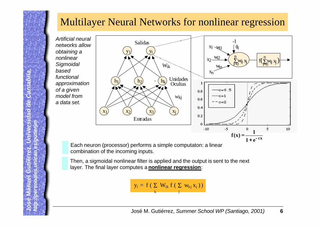
Each neuron (processor) performs a simple computaton: a linear combination of the incoming inputs.

Artificial neural networks allow obtaining a nonlinear Sigmoidalbased functional approximation of a given model from a data set.

wi1

wi2

win

θix1

x2

xn

Σi=0

nwij xj f( )Σi=0

nwij xj

-1

h1 h2 hk

y1 yi

x1 x2 x3 xj

Salidas

Wik

wkj

UnidadesOcultas

Entradas

Multilayer Neural Networks for nonlinear regression

yi = f ( Σk

Wik f (j

wkj xj ) )Σ

Then, a sigmoidal nonlinear filter is applied and the output is sent to the next layer. The final layer computes a nonlinear regression:

cxe1

1)x(f −−++

==


sé

Ma

nu

el

Gu

tié

rre

z, U

niv

ers

ida

d d

e C

an

tab

ria

.Jo

sé M

anu

el G

uti

érre

z, U

niv

ers

ida

d d

e C

an

tab

ria

. h

ttp

://p

erso

nal

es.u

nic

an.e

s/g

uti

erjm

y1 y2 y3

x1 x2 x3 x4

a1p

a2p

a3p

a4p

b1p

b2p

b3p

b1p

b2p

b3p

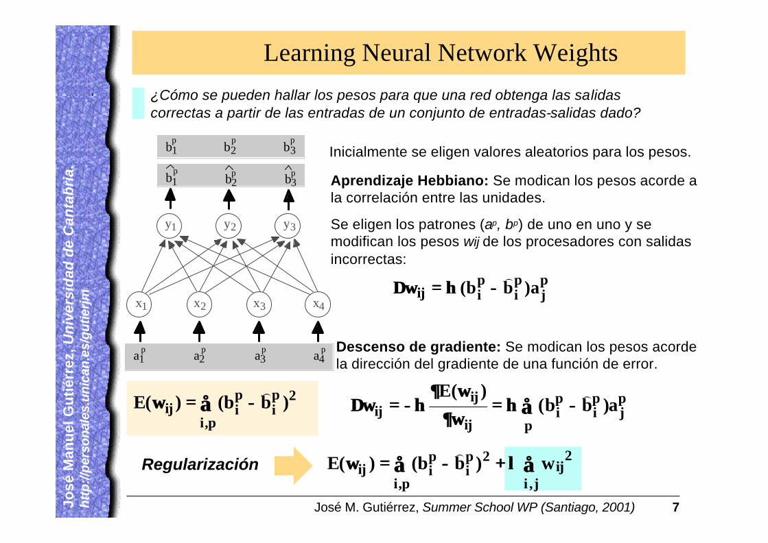
Learning Neural Network Weights

¿Cómo se pueden hallar los pesos para que una red obtenga las salidas correctas a partir de las entradas de un conjunto de entradas-salidas dado?

Inicialmente se eligen valores aleatorios para los pesos.

Aprendizaje Hebbiano: Se modican los pesos acorde a la correlación entre las unidades.

Se eligen los patrones (ap, bp) de uno en uno y se modifican los pesos wij de los procesadores con salidas incorrectas:

pj

pi

piij a)bb(

)−−ηη==ωω∆∆

Descenso de gradiente: Se modican los pesos acorde la dirección del gradiente de una función de error.

∑∑ −−==ωωp,i

2pi

piij )bb()(E

)∑∑ −−ηη==

ωω∂∂ωω∂∂

ηη−−==ωω∆∆p

pj

pi

pi

ij

ijij a)bb(

)(E )

Regularización ∑∑∑∑ λλ++−−==ωωj,i

2ij

p,i

2pi

piij w)bb()(E

)


sé

Ma

nu

el

Gu

tié

rre

z, U

niv

ers

ida

d d

e C

an

tab

ria

.Jo

sé M

anu

el G

uti

érre

z, U

niv

ers

ida

d d

e C

an

tab

ria

. h

ttp

://p

erso

nal

es.u

nic

an.e

s/g

uti

erjm

(b)(a)

x

y

x

y

w11 z1

z2

w12

w22

w21

z1

z2

z3

w11

w12w13w21

w22w23

0.2 0.4 0.6 0.8 1

0.2

0.4

0.6

0.8

1

00 0.2 0.4 0.6 0.8 1

0.2

0.4

0.6

0.8

1

00

(a) (b)

ωx 1

yω2

ωx 1

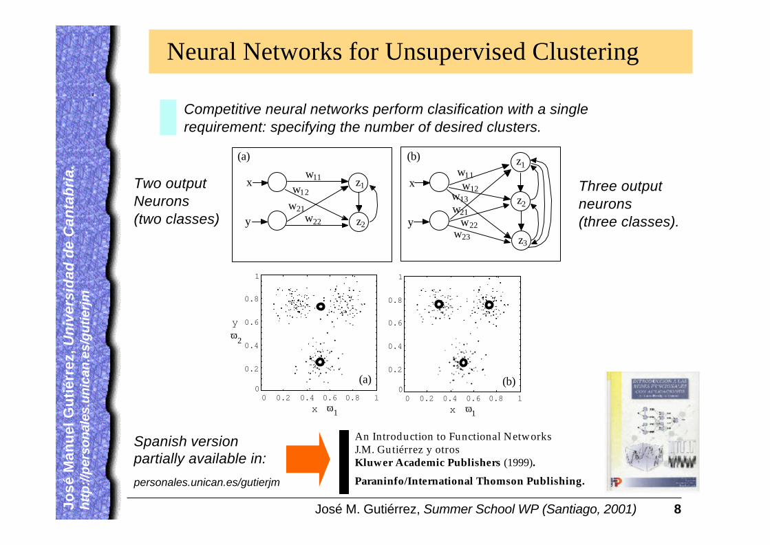
Neural Networks for Unsupervised Clustering

Competitive neural networks perform clasification with a single requirement: specifying the number of desired clusters.

Two outputNeurons (two classes)

Three output neurons (three classes).

An Introduction to Functional NetworksJ.M. Gutiérrez y otrosKluwer Academic Publishers (1999).

Paraninfo/International Thomson Publishing.

Spanish version partially available in:

personales.unican.es/gutierjm


sé

Ma

nu

el

Gu

tié

rre

z, U

niv

ers

ida

d d

e C

an

tab

ria

.Jo

sé M

anu

el G

uti

érre

z, U

niv

ers

ida

d d

e C

an

tab

ria

. h

ttp

://p

erso

nal

es.u

nic

an.e

s/g

uti

erjm

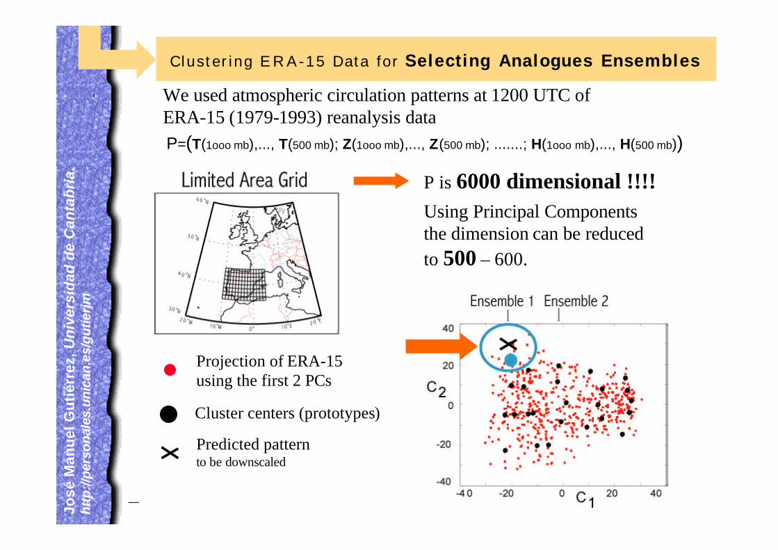
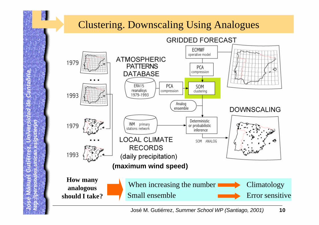
Clustering E R A -15 Data for Selecting Analogues Ensembles

P=(T(1ooo mb),..., T(500 mb); Z(1ooo mb),..., Z(500 mb); .......; H(1ooo mb),..., H(500 mb))

P is 6000 dimensional !!!!Using Principal Components the dimension can be reduced

to 500 – 600.

We used atmospheric circulation patterns at 1200 UTC of ERA-15 (1979-1993) reanalysis data

10% of the ERA data shown

Projection of ERA-15 using the first 2 PCs

Cluster centers (prototypes)

Predicted patternto be downscaled


sé

Ma

nu

el

Gu

tié

rre

z, U

niv

ers

ida

d d

e C

an

tab

ria

.Jo

sé M

anu

el G

uti

érre

z, U

niv

ers

ida

d d

e C

an

tab

ria

. h

ttp

://p

erso

nal

es.u

nic

an.e

s/g

uti

erjm

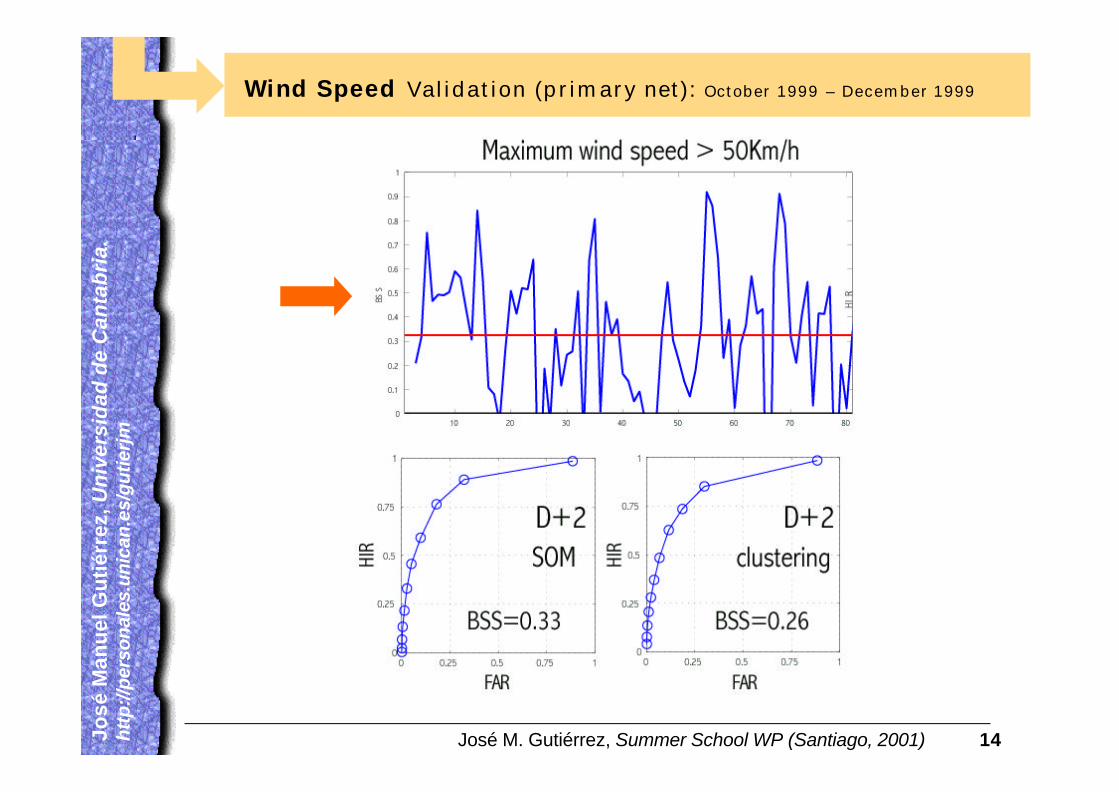
Clustering. Downscaling Using Analogues

How many analogous

should I take?

When increasing the number Climatology

Small ensemble Error sensitive

(maximum wind speed)


sé

Ma

nu

el

Gu

tié

rre

z, U

niv

ers

ida

d d

e C

an

tab

ria

.Jo

sé M

anu

el G

uti

érre

z, U

niv

ers

ida

d d

e C

an

tab

ria

. h

ttp

://p

erso

nal

es.u

nic

an.e

s/g

uti

erjm

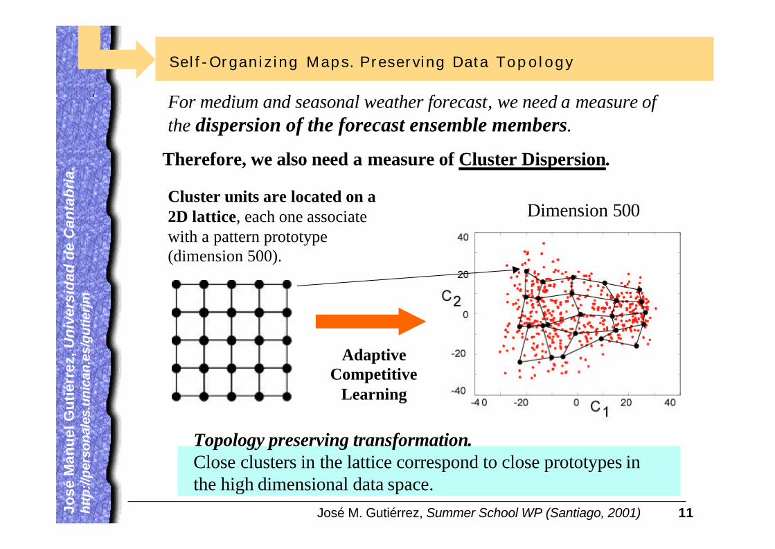
Self - Organizing Maps. Preserving Data Topology

Dimension 500

For medium and seasonal weather forecast, we need a measure of the dispersion of the forecast ensemble members.

Topology preserving transformation.Close clusters in the lattice correspond to close prototypes in the high dimensional data space.

Cluster units are located on a 2D lattice, each one associate with a pattern prototype (dimension 500).

Therefore, we also need a measure of Cluster Dispersion.

Adaptive Competitive

Learning


sé

Ma

nu

el

Gu

tié

rre

z, U

niv

ers

ida

d d

e C

an

tab

ria

.Jo

sé M

anu

el G

uti

érre

z, U

niv

ers

ida

d d

e C

an

tab

ria

. h

ttp

://p

erso

nal

es.u

nic

an.e

s/g

uti

erjm

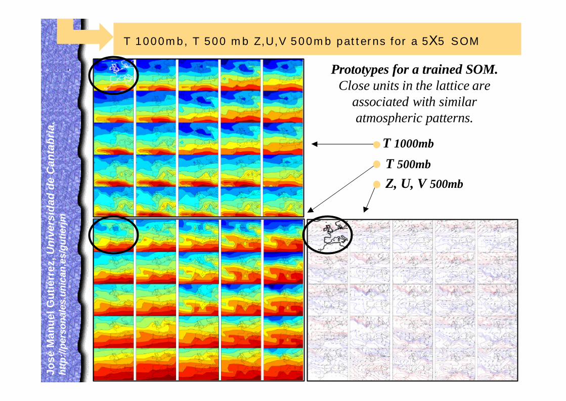
T 1000mb, T 500 mb Z,U,V 500mb patterns for a 5X5 SOM

Prototypes for a trained SOM. Close units in the lattice are

associated with similar atmospheric patterns.

T 1000mb

T 500mb

Z, U, V 500mb


sé

Ma

nu

el

Gu

tié

rre

z, U

niv

ers

ida

d d

e C

an

tab

ria

.Jo

sé M

anu

el G

uti

érre

z, U

niv

ers

ida

d d

e C

an

tab

ria

. h

ttp

://p

erso

nal

es.u

nic

an.e

s/g

uti

erjm

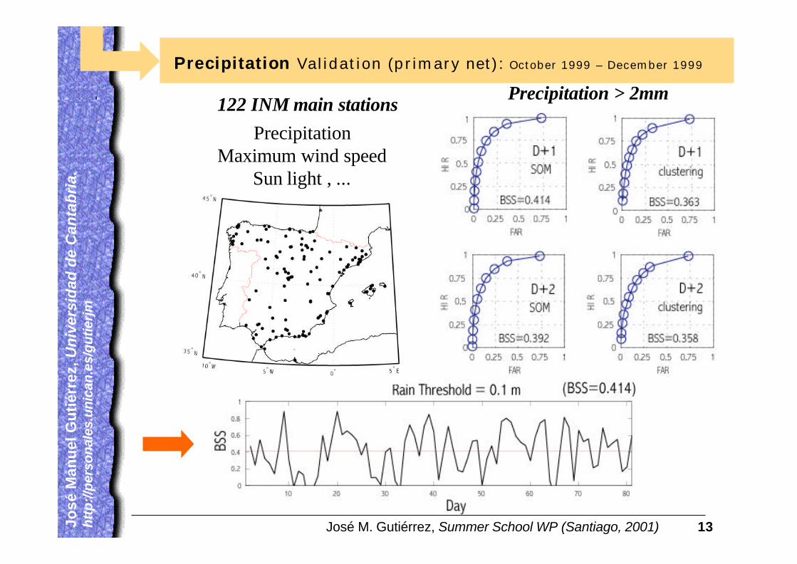
Precipitation Validation (primary net): October 1999 – December 1999

Precipitation > 2mm122 INM main stations

PrecipitationMaximum wind speed

Sun light , ...


sé

Ma

nu

el

Gu

tié

rre

z, U

niv

ers

ida

d d

e C

an

tab

ria

.Jo

sé M

anu

el G

uti

érre

z, U

niv

ers

ida

d d

e C

an

tab

ria

. h

ttp

://p

erso

nal

es.u

nic

an.e

s/g

uti

erjm

Wind Speed Validation (primary net): October 1999 – December 1999


sé

Ma

nu

el

Gu

tié

rre

z, U

niv

ers

ida

d d

e C

an

tab

ria

.Jo

sé M

anu

el G

uti

érre

z, U

niv

ers

ida

d d

e C

an

tab

ria

. h

ttp

://p

erso

nal

es.u

nic

an.e

s/g

uti

erjm

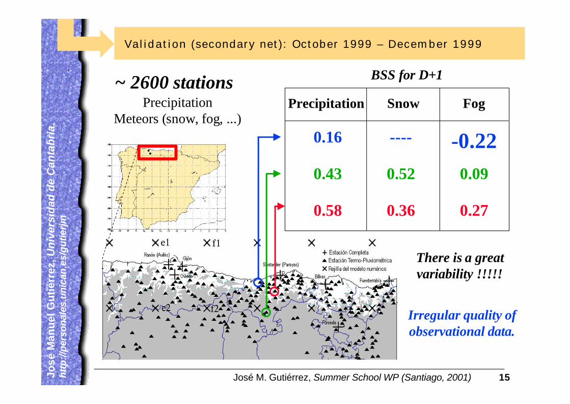
Validation (secondary net): October 1999 – December 1999

~ 2600 stationsPrecipitation

Meteors (snow, fog, ...)Precipitation

0.58

0.43

0.16

0.36

0.52

----

Snow

0.27

0.09

-0.22

Fog

BSS for D+1

There is a great variability !!!!!

Irregular quality of observational data.


sé

Ma

nu

el

Gu

tié

rre

z, U

niv

ers

ida

d d

e C

an

tab

ria

.Jo

sé M

anu

el G

uti

érre

z, U

niv

ers

ida

d d

e C

an

tab

ria

. h

ttp

://p

erso

nal

es.u

nic

an.e

s/g

uti

erjm

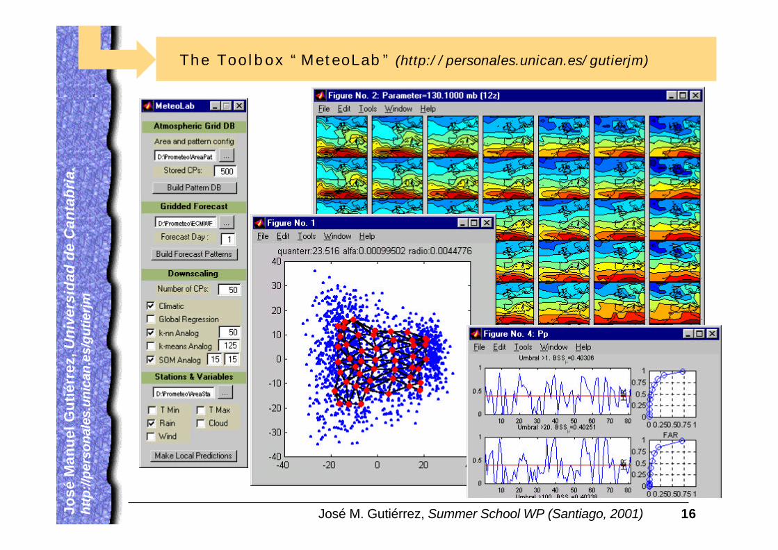
The Toolbox “ MeteoLab ” (http://personales.unican.es/gutierjm)


sé

Ma

nu

el

Gu

tié

rre

z, U

niv

ers

ida

d d

e C

an

tab

ria

.Jo

sé M

anu

el G

uti

érre

z, U

niv

ers

ida

d d

e C

an

tab

ria

. h

ttp

://p

erso

nal

es.u

nic

an.e

s/g

uti

erjm

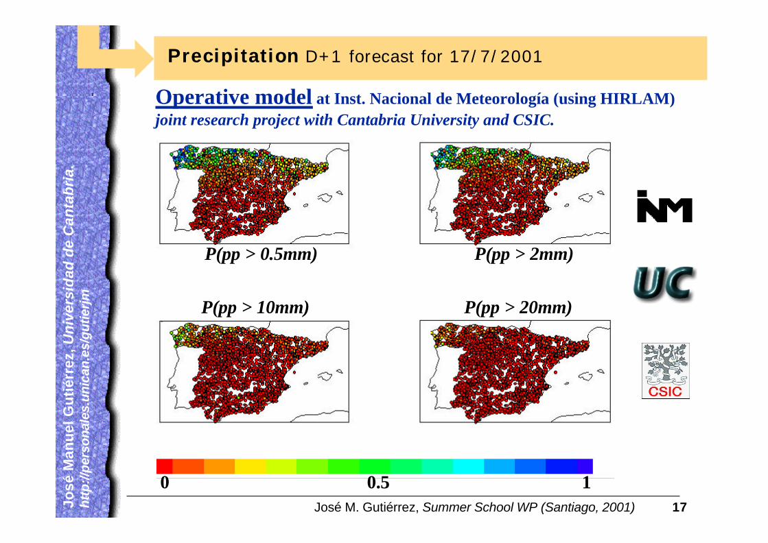
Precipitation D+1 forecast for 17/7/2001

P(pp > 0.5mm)

0 10.5

P(pp > 20mm)P(pp > 10mm)

P(pp > 2mm)

Operative model at Inst. Nacional de Meteorología (using HIRLAM)joint research project with Cantabria University and CSIC.


sé

Ma

nu

el

Gu

tié

rre

z, U

niv

ers

ida

d d

e C

an

tab

ria

.Jo

sé M

anu

el G

uti

érre

z, U

niv

ers

ida

d d

e C

an

tab

ria

. h

ttp

://p

erso

nal

es.u

nic

an.e

s/g

uti

erjm

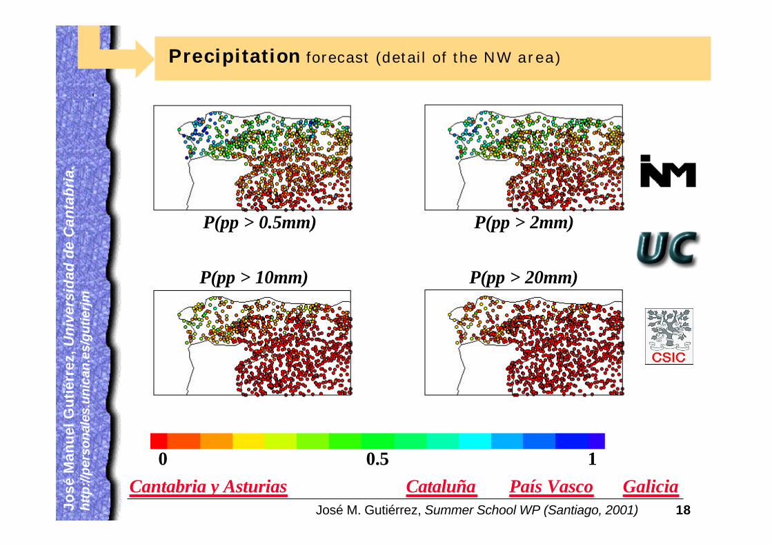
Galicia

P(pp > 0.5mm)

0 10.5

P(pp > 20mm)P(pp > 10mm)

P(pp > 2mm)

Precipitation forecast (detail of the NW area)

País VascoCataluñaCantabria y Asturias


sé

Ma

nu

el

Gu

tié

rre

z, U

niv

ers

ida

d d

e C

an

tab

ria

.Jo

sé M

anu

el G

uti

érre

z, U

niv

ers

ida

d d

e C

an

tab

ria

. h

ttp

://p

erso

nal

es.u

nic

an.e

s/g

uti

erjm

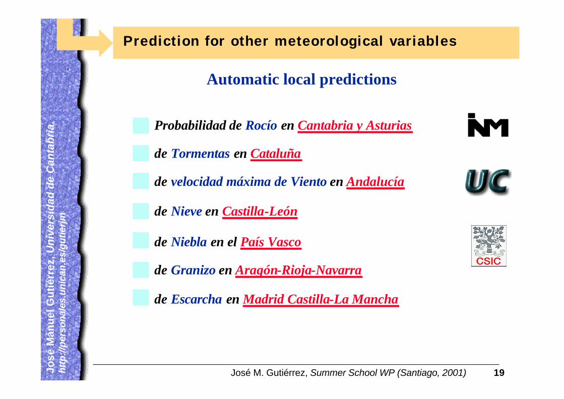
Probabilidad de Rocío en Cantabria y Asturias

Prediction for other meteorological variables

de Tormentas en Cataluña

de velocidad máxima de Viento en Andalucía

de Nieve en Castilla-León

de Niebla en el País Vasco

de Granizo en Aragón-Rioja-Navarra

Automatic local predictions

de Escarcha en Madrid Castilla-La Mancha


sé

Ma

nu

el

Gu

tié

rre

z, U

niv

ers

ida

d d

e C

an

tab

ria

.Jo

sé M

anu

el G

uti

érre

z, U

niv

ers

ida

d d

e C

an

tab

ria

. h

ttp

://p

erso

nal

es.u

nic

an.e

s/g

uti

erjm

Thank you for your attention !!!!!!!!!!!

And sorry for taking two extra minutes.


sé

Ma

nu

el

Gu

tié

rre

z, U

niv

ers

ida

d d

e C

an

tab

ria

.Jo

sé M

anu

el G

uti

érre

z, U

niv

ers

ida

d d

e C

an

tab

ria

. h

ttp

://p

erso

nal

es.u

nic

an.e

s/g

uti

erjm

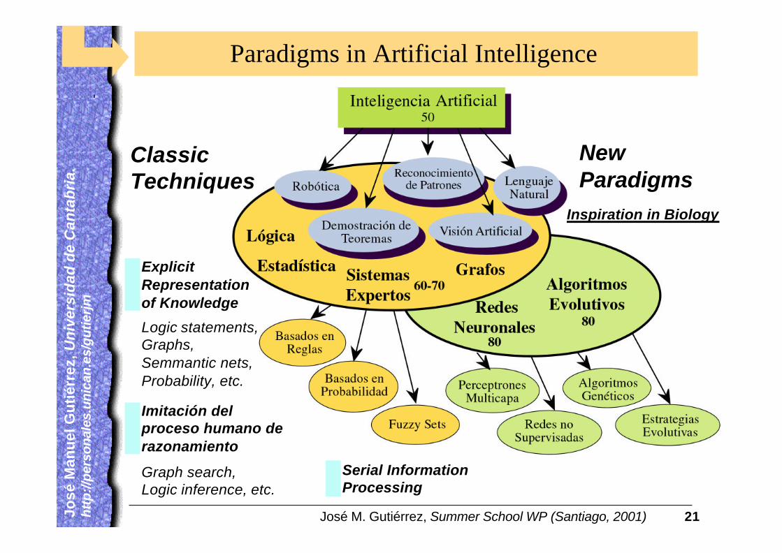
Paradigms in Artificial Intelligence

Classic Techniques

New Paradigms

Inspiration in Biology

Explicit Representation of Knowledge

Imitación del proceso humano de razonamiento

Serial Information Processing

Logic statements,Graphs,Semmantic nets,Probability, etc.

Graph search,Logic inference, etc.


sé

Ma

nu

el

Gu

tié

rre

z, U

niv

ers

ida

d d

e C

an

tab

ria

.Jo

sé M

anu

el G

uti

érre

z, U

niv

ers

ida

d d

e C

an

tab

ria

. h

ttp

://p

erso

nal

es.u

nic

an.e

s/g

uti

erjm

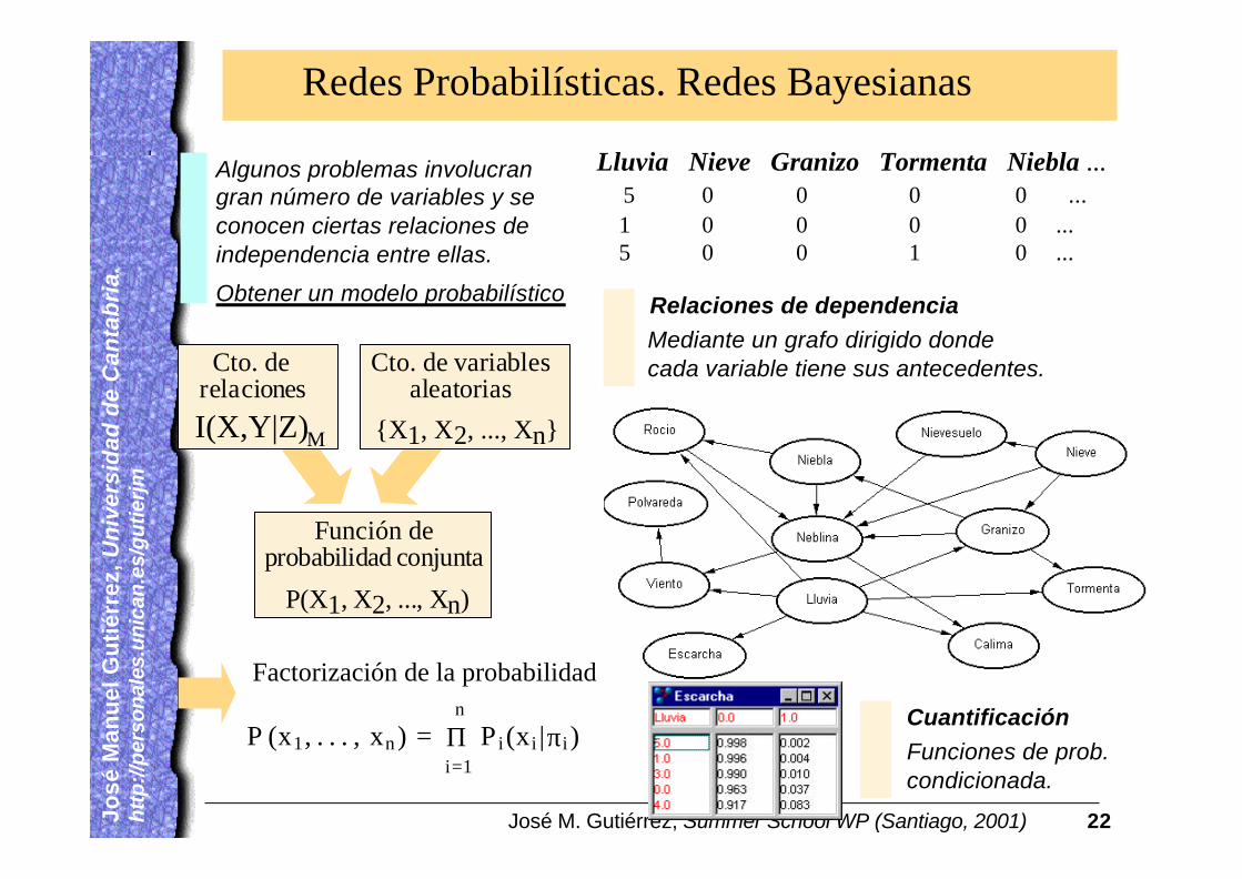
Redes Probabilísticas. Redes Bayesianas

Algunos problemas involucran gran número de variables y se conocen ciertas relaciones de independencia entre ellas.

Obtener un modelo probabilístico

P(X1, X2, ..., Xn)

Función deprobabilidad conjunta

{X1, X2, ..., Xn}

Cto. de variablesaleatorias

I(X,Y|Z)M

Cto. derelaciones

Factorización de la probabilidad !!

P (x1, . . . , xn ) =n

i=1

P i(x i |πi)Π

Lluvia Nieve Granizo Tormenta Niebla ...5 0 0 0 0 ...1 0 0 0 0 ...5 0 0 1 0 ...

Relaciones de dependencia

Mediante un grafo dirigido donde cada variable tiene sus antecedentes.

Cuantificación

Funciones de prob.condicionada.


sé

Ma

nu

el

Gu

tié

rre

z, U

niv

ers

ida

d d

e C

an

tab

ria

.Jo

sé M

anu

el G

uti

érre

z, U

niv

ers

ida

d d

e C

an

tab

ria

. h

ttp

://p

erso

nal

es.u

nic

an.e

s/g

uti

erjm

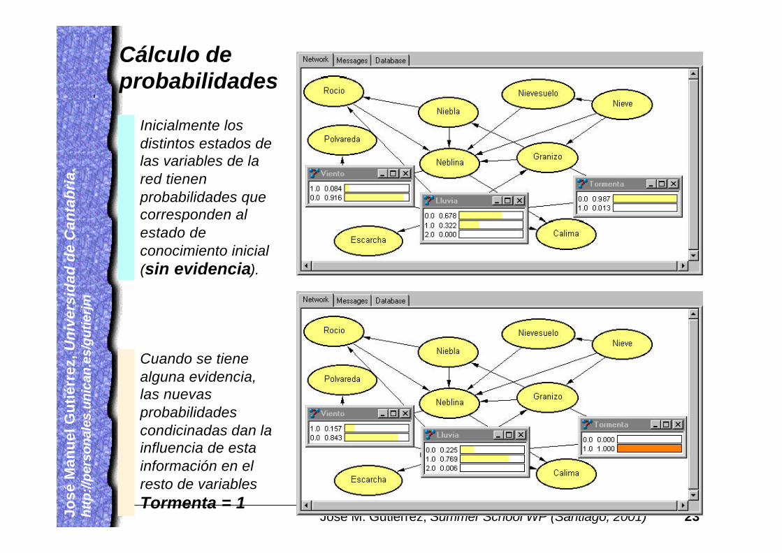
Inicialmente los distintos estados de las variables de la red tienen probabilidades que corresponden al estado de conocimiento inicial (sin evidencia).

Cuando se tiene alguna evidencia, las nuevas probabilidades condicinadas dan la influencia de esta información en el resto de variablesTormenta = 1

Cálculo de probabilidades

statistical and machine learning techniques for...

Documents