STATISTICAL ANALYSIS OFGROUND-WATER MONITORING DATA

AT RCRA FACILITIES

INTERIM FINAL GUIDANCE

OFFICE OF SOLID WASTEWASTE MANAGEMENT DIVISIONU.S. ENVIRONMENTAL PROTECTION AGENCY401 M STREET, S.W.WASHINGTON, D.C.20460

APRIL 1989

DISCLAIMER

This document is intended to assist Regional and State personnel inevaluating ground-water monitoring data from RCRA facilities. Conformancewith this guidance is expected to result in statistical methods and samplingprocedures that meet the regulatory standard of protecting human health andthe environment. However, EPA will not in all cases limit its approval ofstatistical methods and sampling procedures to those that comport with theguidance set forth herein. This guidance is not a regulation (i.e., it doesnot establish a standard of conduct which has the force of law) and should notbe used as such. Regional and State personnel should exercise their discre-tion in using this guidance document as well as other relevant information inchoosing a statistical method and sampling procedure that meet the regulatoryrequirements for evaluating ground-water monitoring data from RCRA facilities.

This document has been reviewed by the Office of Solid Waste, U.S. Envi-ronmental Protection Agency, Washington, D.C., and approved for publication.Approval does not signify that the contents necessarily reflect the views andpolicies of the U.S. Environmental Protection Agency, nor does mention oftrade names, commercial products, or publications constitute endorsement orrecommendation for use.

Guidance Document on the StatisticaI Analysisof Ground-Water Monitoring Data

at RCRA Facilities

PREFACE

This guidance document has been developed primarily for evaluatingground-water monitoring data at RCRA (Resource Conservation and Recovery Act)facilities. The statistical methodologies described in this document can beapplied to both hazardous (Subtitle C of RCRA) and municipal (Subtitle D ofRCRA) waste land disposal facilities.

The recently amended regulations concerning the statistical analysis ofground-water monitoring data at RCRA facilities (53 FR 39720, October 11,1988), provide a wide variety of statistical methods that may be used toevaluate ground-water quality. To the experienced and inexperienced waterquality professional, the choice of which test to use under a particular setof conditions may not be apparent. The reader is referred to Section 4 ofthis guidance, "Choosing a Statistical Method," for assistance in choosing anappropriate statistical test. For relatively new facilities that have onlylimited amounts of ground-water monitoring data, it is recommended that a formof hypothesis test (e.g., parametric analysis of variance) be employed toevaluate the data. Once sufficient data are available (after 12 to 24 monthsor eight background samples), another method of analysis such as the controlchart methodology described in Section 7 of the guidance is recommended. Eachmethod of analysis and the conditions under which they will be used can bewritten in the facility permit. This will eliminate the need for a permitmodification each time more information about the hydrogeochemistry iscollected, and more appropriate methods of data analysis become apparent.

This guidance was written primarily for the statistical analysis ofground-water monitoring data at RCRA facilities. The guidance has widerapplications however, if one examines the spatial relationships involvedbetween the monitoring wells and the potential contaminant source. Forexample, Section 5 of the guidance describes background well (upgradient) vs.compliance well (downgradient) comparisons. This scenario can be applied toother non-RCRA situations involving the same spatial relationships and thesame null hypothesis.between means, or where

The explicit null hypothesis (Ho) for testing contrastsappropriate between medians, is that the means between

groups (here monitoring wells) are equal (i.e., no release has been detected),or that the group means are below a prescribed action level (e.g., the ground-water protection standard). Statistical methods that can be used to evaluatethese conditions are described in Section 5.2 (Analysis of Variance), 5.3(Tolerance Intervals), and 5.4 (Prediction Intervals).

A different situation exists when compliance wells (downgradient) arecompared to a fixed standard (e.g., the ground-water protection standard). Inthat case, Section 6 of the guidance should be consulted. The value to whichthe constituent concentrations at compliance wells are compared can be any

iii

standard established by a Regional Administrator, State or county healthofficial, or another appropriate official.

A note of caution applies to Section 6. The examples used in Section 6are used to determine whether ground water has been contaminated as a resultof a release from a facility. When the lower confidence limit lies entirelyabove the ACL (alternate concentration limit) or MCL (maximum concentrationlimit), further action or assessment may be warranted. If one wishes todetermine whether a cleanup standard has been attained for a Superfund site ora RCRA facility in corrective action, another EPA guidance document entitled,"Statistical Methods for the Attainment of Superfund Cleanup Standards (Vol-ume 2: Ground Water--Draft), should be consulted. This draft Superfundguidance is a multivolume set that addresses questions regarding the successof air, ground-water, and soil remediation efforts. Information about theavailability of this draft guidance, currently being developed, can beobtained by calling the RCRA/Superfund Hotline, telephone (800) 424-9346 or(202) 382-3000.

Those interested in evaluating individual uncontaminated wells or in anintrawell comparison are referred to Section 7 of the guidance which describesthe use of Shewhart-CUSUM control charts and trend analysis. Municipal watersupply engineers, for example, who wish to monitor water quality parameters insupply wells, may find this section useful.

Other sections of this guidance have wide applications in the field ofapplied statistics, regardless of the intended use or purpose. Section 4.2and 4.3 provide information on checking distributional assumptions andequality of variance, while Sections 8.1 and 8.2 cover limit of detectionproblems and outliers. Helpful advice and references for many experimentsinvolving the use of statistics can be found in these sections.

Finally, it should be noted that this guidance is not intended to be thefinal chapter on the statistical analysis of ground-water monitoring data, norshould it be used as such. 40 CFR Part 264 Subpart F offers an alternative§5264.97(h)(5)] to the methods suggested and described in this guidancedocument. In fact, the guidance recommends a procedure (confidence intervals)for comparing monitoring data to a fixed standard that is not mentioned in theSubpart F regulations. This is neither contradictory nor inconsistent, butrather epitomizes the complexities of the subject matter and exemplifies theneed for flexibility due to the-site-specific monitoring requirements of theRCRA program.

iv

CONTENTS

Preface... . .

.......... ..................................................... 111Figures . . . . . . . . . . . . . . . . . . . . . . . . . . . . . . . . . . . . . . . . . . . . . . . . . . . . . . . . . . . . . . . . . viTables . . . . . . . . . . . . . . . . . . . . . . . . . . . . . . . . . . . . . . . . . . . . . . . . . . . . . . . . . . . . . . . . . . viiExecutive Summary . . . . . . . . . . . . . . . . . . . . . . . . . . . . . . . . . . . . . . . . . . . . . . . . . . . . . . . E-l

1.2.

3.

4.

5.

6.

7.

8.

Introduction ..................................................Regulatory Overview ...........................................

2.1 Background ..........................................2.2 Overview of Methodology .............................2.3 General Performance Standards .......................2.4 Basic Statistical Methods and Sampling

Procedures ........................................Choosing a Sampling Interval ..................................

3.1 Example Calculations ................................3.2 Flow Through Karst and "Pseudo-Karst" Terranes ......

Choosing a Statistical Method .................................4.1 Flowcharts--Overview and Use ........................4.2 Checking Distributional Assumptions .................4.3 Checking Equality,of Variance: Bartlett's Test .....

Background Well to Compliance Well Comparisons ................5.1 Summary Flowchart for Background Well to

Compliance Well Comparisons .......................5.2 Analysis of Variance ................................5.3 Tolerance Intervals Based on the Normal

Distribution ......................................5.4 Prediction Intervals................................

Comparisons with MCLs or ACLs .................................6.1 Summary Chart for Comparison with MCLs or ACLs ......6.2 Statistical Procedures ..............................

Control Charts for Intra-Well Comparisons .....................7.1 Advantages of Plotting Data .........................7.2 Correcting for Seasonality ..........................7.3 Combined Shewhart-CUSUM Control Charts for Each

Well and Constituent ..............................7.4 Update of a Control Chart ...........................7.5 Nondetects in a Control Chart .......................

Miscellaneous Topics ..........................................8.1 Limit of Detection ..................................8.2 Outliers ............................................

2-63-13-8

3-114-14-14-4

4-175-1

5-25-5

5-205-246-16- l6-17- l7-17-2

7-107-12

8-18-11

AppendicesA. General Statistical Considerations and Glossary of

Statistical Terms . . . . . . . . . . . . . . . . . . . . . . . . . . . . . . . . . . . . . . . . . . . A-l

B.Statistical Tables . . . . . . . . . . . . . . . . . . . . . . . . . . . . . . . . . . . . . . . . . . . . B-lGeneral Bibliography . . . . . . . . . . . . . . . . . . . . . . . . . . . . . . . . . . . . . . . . . . C-l

C. Federal Register, 40 CFR, Part 264 . . . . . . . . . . . . . . . . . . . . . . . . . . . . . D-l

V

FIGURES

Page

Hydraulic conductivity of selected rocks...................... 3-3

Range of values of hydraulic conductivity and permeability.... 3-4

Number

3-l

3-2

3-3

3-4

3-5

4-l

4-2

4-3

5-1

5-2

6-1 Comparisons with MCLs/ACLs . . . . . . . . . . . . . . . . . . . . . . . . . . . . . . . . . . . . 6-2

7-1 Plot of unadjusted and seasonally adjusted monthlyobservations . . . . . . . . . . . . . . . . . . . . . . . . . . . . . . . . . . . . . . . . . . . . . . . . 7-6

7-2 Combined Shewhart-CUSUM chart . . . . . . . . . . . . . . . . . . . . . . .......... 7-11

Conversion factors for permeability and hydraulicconductivity units . . . ...................................... 3-4

Total porosity and drainable porosity for typicalgeologic materials . . . . . . . . . . . . . . . . . . . . . . . . . . . . . . . . . . . . . . . . . . 3-7

Potentiometric surface map for computation of hydraulicgradient . . . ........................................... 3-9

Flowchart overview . . . . . . . . . . . . . . . . . . . . . . . . . . . . . . . . . . . . . . . . . . . . 4-3

Probability plot of raw chlordane concentrations.............. 4-11

Probability plot of log-transformed chlordane concentrations.. 4-13

Background well to compliance well comparisons................ 5-3

Tolerance limits: alternate approach to backgroundwell to compliance well comparisons......................,.. 5-4

vi

TABLES

Number Page

2-1 Summary of Statistical Methods . . . . . . . . . . . . . . . . . . . . . . . . . . . . . . . . 2-7

3-1 Default Values for Effective Porosity (Ne) for Use in Timeof Travel (TOT) Analyses .................................... 3-5

3-2 Specific Yield Values for Selected Rock Types ................. 3-6

3-3 Determining a Sampling Interval ............................... 3-11

4-1 Example Data for Coefficient-of-Variation Test ................ 4-8

4-2 Example Data Computations for Probability Plotting ............ 4-10

4-3 Cell Boundaries for the Chi-Squared Test ...................... 4-14

4-4 Example Data for Chi-Squared Test ............................. 4-15

4-5 Example Data for Bartlett's Test .............................. 4-19

5-l One-Way Parametric ANOVA Table ................................ s-a

5-2 Example Data for One-Way Parametric Analysis of Variance ...... 5-11

5-3 Example Computations in One-Way Parametric ANOVA Table ........ 5-12

5-4 Example Data for One-Way Nonparametric ANOVA--BenzeneConcentrations (ppm) ........................................ 5-18

5-5 Example Data for Normal Tolerance Interval .................... 5-23

5-6 Example Data for Prediction Interval--Chlordane Levels ........ 5-27

6-l Example Data for Normal Confidence Interval--AldicarbConcentrations in Compliance Wells (ppb) .................... 6-4

6-2 Example Data for Log-Normal Confidence Interval--EDBConcentrations in Compliance Wells (ppb) .................... 6-6

6-3 Values of M and n+l-M and Confidence Coefficients forSmall Samples ............................................... 6-9

6-4 Example Data for Nonparametric Confidence Interval--T-29Concentrations (ppm) ........................................ 6-10

vii

TABLES (continued)

Number

6-5

7-l

7-2

8-l

8-2

8-3

8-4

Page

Example Data for a Tolerance Interval Compared to an ACL ...... 6-13

Example Computation for Deseasonalizing Data ................. 7-4

Example Data for Combined Shewhart-CUSUM Chart--CarbonTetrachloride Concentration (µg/L) .......................... 7-9

Methods for Below Detection Limit Values ...................... 8-2

Example Data for a Test of Proportions ........................ 8-6

Example Data for Testing Cohen's Test ......................... 8-9

Example Data for Testing for an Outlier ....................... 8-13

viii

ACKNOWLEDGMENT

This document was developed by EPA's Office of Solid Waste under thedirection of Dr. Vernon Myers, Chief of the Ground-Water Section of the WasteManagement Division. The document was prepared by the joint efforts ofDr. Vernon B. Myers, Mr. James R. Brown of the Waste Management Division,Mr. James Craig of the Office of Policy Planning and Information, andMr. Barnes Johnson of the Office of Policy, Planning, and Evaluation. Tech-nical support in the preparation of this document was provided by MidwestResearch Institute- (MRI) under a subcontract to NUS Corporation, the primecontractor with EPA's Office of Solid Waste. MRI staff who assisted with thepreparation of the document were Jairus 0. Flora, Jr., Ph.D., PrincipalStatistician, Ms. Karin M. Bauer, Senior Statistician, and Mr. Joseph S.Bartling, Assistant Statistician.

ix

EXECUTIVE SUMMARY

The hazardous waste regulations under the Resource Conservation andRecovery Act (RCRA) require owners and operators of hazardous waste facilitiesto utilize design features and control measures that prevent the release ofhazardous waste into ground. water. Further, regulated units (i.e., all sur-face impoundments, waste piles, land treatment units, and landfills thatreceive hazardous waste after July 26, 1982) are also subject to the ground-water monitoring and corrective action standards of 40 CFR Part 264, Sub-part F. These regulations require that a statistical method and sampling pro-cedure approved by EPA be used to determine whether there are releases fromregulated units into ground water.

This document provides guidance to RCRA facility permit applicants andwriters concerning the statistical analysis of ground-water monitoring data atRCRA facilities. Section 1 is an introduction to the guidance; it describesthe purpose and intent of the document and emphasizes the need for site-specific considerations in implementing the Subpart F regulations of 40 CFRPart 264.

Section 2 provides the reader with an overview of the recently promul-gated regulations concerning the statistical analysis of ground-water moni-toring data (53 FR 39720, October 11, 1988).regulation are reviewed,

The requirements of theand the need to consider site-specific factors in

evaluating data at a hazardous waste facility is emphasized.

Section 3 discusses the important hydrogeologic parameters to considerwhen choosing a sampling interval. The Darcy equation is used to determinethe horizontal component of the average linear velocity of ground water. Thisparameter provides a good estimate of time of travel for most soluble con-stituents in ground water and may be used to determine a sampling interval.In karst, cavernous volcanics, and fractured geologic environments, alterna-tive methods are needed to determine an appropriate sampling interval. Exam-ple calculations are provided at the end of the section to further assist thereader.

Section 4 provides guidance on choosing an appropriate statisticalmethod. A flow chart to guide the reader through this section, as well asprocedures to test the distributional assumptions of data, are presented.Finally, this section outlines procedures to test specifically for equality ofvariance.

Section 5 covers statistical methods that may be used to evaluate ground-water monitoring data when background wells have been sited hydraulicallyupgradient from the regulated unit, and a second set of wells are sited

E-l

hydraulically downgradient from the regulated unit at the point of compli-ance. The data from these compliance wells are compared to data from thebackground wells to determine whether a release from a facility hasoccurred. Parametric and nonparametric analysis of variance, tolerance inter-vals, and prediction intervals are suggested methods for this type of compari-son. Flow charts, procedures,testing method.

and example calculations are given for each

Section 6 includes statistical procedures that are appropriate whencomparing ground-water constituent concentrations to fixed concentrationlimits (e.g., alternate concentration limits or maximum concentration lim-its). The methods applicable to this type of comparison are confidence inter-vals and tolerance intervals. As in Section 5, flow charts, procedures, andexamples explain the calculations necessary for each testing method.

Section 7 presents the case where the level of each constituent within asingle, uncontaminated well is being compared to its historic background con-centrations. This is known as an intra-well comparison. In essence, the datafor each constituent in each well are plotted on a time scale and inspectedfor obvious features such as trends or sudden changes in concentrationlevels. The method suggested in this section is a combined Shewhart-CUSUMcontrol chart.

Section 8 contains a variety of special topics that are relatively shortand self-contained. These topics include methods to deal with data that isbelow the limit of analytical detection and methods to test for outliers orextreme values in the data.

Finally, the guidance presents appendices that cover general statisticalconsiderations, a glossary of statistical terms,listing of references.

statistical tables, and aThese appendices provide necessary and ancillary

information to aid the user in evaluating ground-water monitoring data.

E-2

SECTION 1

INTRODUCTION

The U.S. Environmental Protection Agency (EPA) promulgated regulationsfor detecting contamination of ground water at hazardous waste land disposalfacilities under the Resource Conservation and Recovery Act (RCRA) of 1976.The statistical procedures specified for use to evaluate the presence of con-tamination have been criticized and require improvement. Therefore, EPA hasrevised those statistical procedures in 40 CFR Part 264, "Statistical Methodsfor Evaluating Ground-Water Monitoring Data From Hazardous Waste Facilities."

In 40 CFR Part 264, EPA has recently amended the Subpart F regulationswith statistical methods and sampling procedures that are appropriate forevaluating ground-water monitoring data under a variety of situations (53 FR39720, October 11, 1988). The purpose of this document is to provide guidancein determining which situation applies and consequently which statisticalprocedure may be used. In addition to providing guidance on selection of anappropriate statistica. procedure, this document provides instructions oncarrying out the procedure and interpreting the results.

The regulations provide three levels of monitoring for a regulatedunit: detection monitoring; compliance monitoring; and corrective action.The regulations define conditions for a regulated unit to be changed from onelevel of monitoring to a more stringent level of monitoring (e.g., from detec-tion monitoring to compliance monitoring). These conditions are that there isstatistically significant evidence of contamination [40 CFR §264.91(a)(l) and(2)].

The regulations allow the benefit of the doubt to reside with the currentstage of monitoring. That is, a unit will remain in its current monitoringstage unless there is convincing evidence to change it. This means that aunit will not be changed from detection monitoring to compliance monitoring(or from compliance monitoring to corrective action) unless there is statisti-cally significant evidence of contamination (or contamination above the com-pliance limit).

The main purpose of this document is to guide owners, operators, RegionalAdministrators, State Directors, and other interested parties in the selec-tion, use, and interpretation of appropriate statistical methods for monitor-ing the ground water at each specific regulated unit. Topics to be coveredinclude sampling needed, sample sizes, selection of appropriate statisticaldesign, matching analysis of data to design, and interpretation of results.Specific recommended methods are detailed and a general discussion of evalu-ation of alternate methods is provided. Statistical concepts are discussed in

l-l

Appendix A. References for suggested procedures are provided as well asreferences to alternate procedures and general statistics texts. Situationscalling for external consultation are mentioned as well as sources for obtain-ing expert assistance when needed.

EPA would like to emphasize the need for site-specific considerations inimplementing the Subpart F regulations of 40 CFR Part 264 (especially asamended, 53 FR 39720, October 11, 1988). It has been an ongoing strategy topromulgate regulations that are specific enough to implement, yet flexibleenough to accommodate a wide variety of site-specific environmental factors.This is usually achieved by specifying criteria that are appropriate for themajority of monitoring situations, while at the same-time allowing alterna-tives that are also protective of human health and the environment. Thisphilosophy is maintained in the recently promulgated amendments entitled,"Statistical Methods for Evaluating Ground-Water Monitoring Data From Haz-ardous Waste Facilities" (53 FR 39720, October 11, 1988). The sections thatallow for the use of an alternate sampling procedure and statistical method[§264.97(g)(2) and §264.97(h)(5), respectively] are as viable as those thatare explicitly referenced [§264.97(g)(l) and §264.97(h)(l-4)], provided theymeet the performance standards of §264.97(i). Due consideration to thisshould be given when preparing and reviewing Part B permits and permitapplications.

l-2

SECTION 2

REGULATORY OVERVIEW

In 1982, EPA promulgated ground-water monitoring and response standardsfor permitted facilities in Subpart F of 40 CFR Part 264, for detectingreleases of hazardous wastes into ground water from storage, treatment, anddisposal units, at permitted facilities (47 FR 32274, July 26, 1982).

The Subpart F regulations required ground-water data to be examined byCochran's Approximation to the Behrens-Fisher Student's t-test (CABF) todetermine whether there was a significant exceedance of background levels, orother allowable levels, of specified chemical parameters and hazardous wasteconstituents. One concern was that this procedure could result in a high rateof "false positives" (Type I error), thus requiring an owner or operatorunnecessarily to advance into a more comprehensive and expensive phase ofmonitoring. More importantly, another concern was that the procedure couldresult in a high rate of "false negatives" (Type II error), i.e., instanceswhere actual contamination would go undetected.

As a result of these concerns, EPA amended the CABF procedure with fivedifferent statistical methods that are more appropriate for ground-water moni-toring (53 FR 39720, October 11, 1988). These amendments also outline sam-pling procedures and performance standards that are designed to help minimizethe event that a statistical method will indicate contamination when it is notpresent (Type I error), and fail to detect contamination when it is present(Type II error).

2.1 BACKGROUND

Subtitle C of the Resource Conservation Recovery Act of 1976 (RCRA) cre-ates a comprehensive program for the safe management of hazardous waste. Sec-tion 3004 of RCRA requires owners and operators of facilities that treat,store, or dispose of hazardous waste to comply with standards established byEPA that are "necessary to protect human health and the environment." Sec-tion 3005 provides for implementation of these standards under permits issuedto owners and operators by EPA or authorized States. Section 3005 also pro-vides that owners and operators of existing facilities that apply for a permitand comply with applicable notice requirements may operate until a permitdetermination is made. These facilities are commonly known as "interimstatus" facilities. Owners and operators of interim status facilities alsomust comply with standards set under Section 3004.

EPA promulgated ground-water monitoring and response standards for per-mitted facilities in 1982 (47 FR 32274, July 26, 1982), codified in 40 CFR

2-l

Part 264, Subpart F. These standards establish programs for protecting groundwater from releases of hazardous wastes from treatment, storage, and disposalunits. Facility owners and operators were required to sample ground water atspecified intervals and to use a statistical procedure to determine whether ornot hazardous wastes or constituents from the facility are contaminatingground water. As explained in more detail below, the Subpart F regulationsregarding statistical methods used in evaluating ground-water monitoring datathat EPA promulgated in 1982 have generated criticism.

The Part 264 regulations prior to the October 11, 1988 amendments pro-vided that the Cochran's Approximation to the Behrens-Fisher Student's t-test(CABF) or an alternate statistical procedure approved by EPA be used to deter-mine whether there is a statistically significant exceedance of backgroundlevels, or other allowable levels, of specified chemical parameters and haz-ardous waste constituents. Although the regulations have always providedlatitude for the use of an alternate statistical procedure, concerns wereraised that the CABF statistical procedure in the regulations was not appro-priate. It was pointed out that: (1) the replicate sampling method is notappropriate for the CABF procedure, (2) the CABF procedure does not adequatelyconsider the number of comparisons that must be made, and (3) the CABF doesnot control for seasonal variation. Specifically, the concerns were that theCABF procedure could result in "false positives" (Type I error), thus requir-ing an owner or operator unnecessarily to collect additional ground-watersamples, to further characterize ground-water quality, and to apply for apermit modification, which is then subject to EPA review. In addition, therewas concern that CABF may result in "false negatives" (Type II error), i.e.,instances where actual contamination goes undetected. This could occurbecause the background data, which are often used as the basis of thestatistical comparisons, are highly variable due to temporal, spatial,analytical, and sampling effects.

As a result of these concerns, on October 11, 1988 EPA amended both thestatistical methods and the sampling procedures of the regulations, by requir-ing (if necessary) that owners or operators more accurately characterize thehydrogeology and potential contaminants at the facility, and by including inthe regulations performance standards that all the statistical methods andsampling procedures must meet. Statistical methods and sampling proceduresmeeting these performance standards would have a low probability of indicatingcontamination when it is not present, and of failing to detect contaminationthat actually is present. The facility owner or operator would have to demon-strate that a procedure is appropriate for the site-specific conditions at thefacility, and to ensure that it meets the performance standards outlinedbelow. This demonstration holds for any of the statistical methods and sam-pling procedures outlined in this regulation as well as any alternate methodsor procedures proposed by facility owners and operators.

EPA recognizes that the selection of appropriate monitoring parameters isalso an essential part of a reliable statistical evaluation. The Agencyaddressed this issue in a previous Federal Register notice (52 FR 25942,July 9, 1987).

2-2

2.2 OVERVIEW OF METHOOOLOGY

EPA has elected to retain the idea of general performance requirementsthat the regulated community must meet. This approach allows for flexibilityin designing statistical methods and sampling procedures to site-specificconsiderations.

EPA has tried to bring a measure of certainty to these methods, whileaccommodating the unique nature of many of the regulated units in question.Consistent with this general strategy, the Agency is establishing severaloptions for the sampling procedures and statistical methods to be used indetection monitoring and, where appropriate, in compliance monitoring.

The owner or operator shall submit, for each of the chemical parametersand hazardous constituents listed in the facility permit, one or more of thestatistical methods and sampling procedures described in the regulationspromulgated on October -11, 1988. In deciding which statistical test isappropriate, he or she will consider the theoretical properties of the test,the data available, the site hydrogeology, and the fate and transport charac-teristics of potential contaminants at the facility. The Regional Administra-tor will review, and if appropriate, approve the proposed statistical methodsand sampling procedures when issuing the facility permit.

The Agency recognizes that there may be situations where any one statis-tical test may not be appropriate. This is true of new facilities with littleor no ground-water monitoring data. If insufficient data prohibit the owneror operator from specifying a statistical method of analysis, then contingencyplans containing several methods of data analysis and the conditions underwhich the method can be used will be specified by the Regional Administratorin the permit. In many cases, the parametric ANOVA can be performed after sixmonths of data have been collected. This will eliminate the need for a permitmodification in the event that data collected during future sampling andanalysis events indicate the need to change to a more appropriate statisticalmethod of analysis. In the event that a permit modification is necessary tochange a sampling procedure or a statistical method, the reader is referred to53 FR 37912, September 28, 1988. These are considered Class 1 changes requir-ing Director approval and should follow minor modification procedures.

2.3 GENERAL PERFORMANCE STANDARDS

EPA's basic concern in establishing these performance standards for sta-tistical methods is to achieve a proper balance between the risk that the pro-cedures will falsely indicate that a regulated unit is causing backgroundvalues or concentration limits to be exceeded (false positives) and the riskthat the procedures will fail to indicate that background values or concen-tration limits are being exceeded (false negatives). EPA's approach isdesigned to address that concern directly. Thus any statistical method orsampling procedure, whether specified here or as an alternative to thosespecified, should meet the following performance standards contained in40 CFR §264.97(i):

2-3

1.

2.

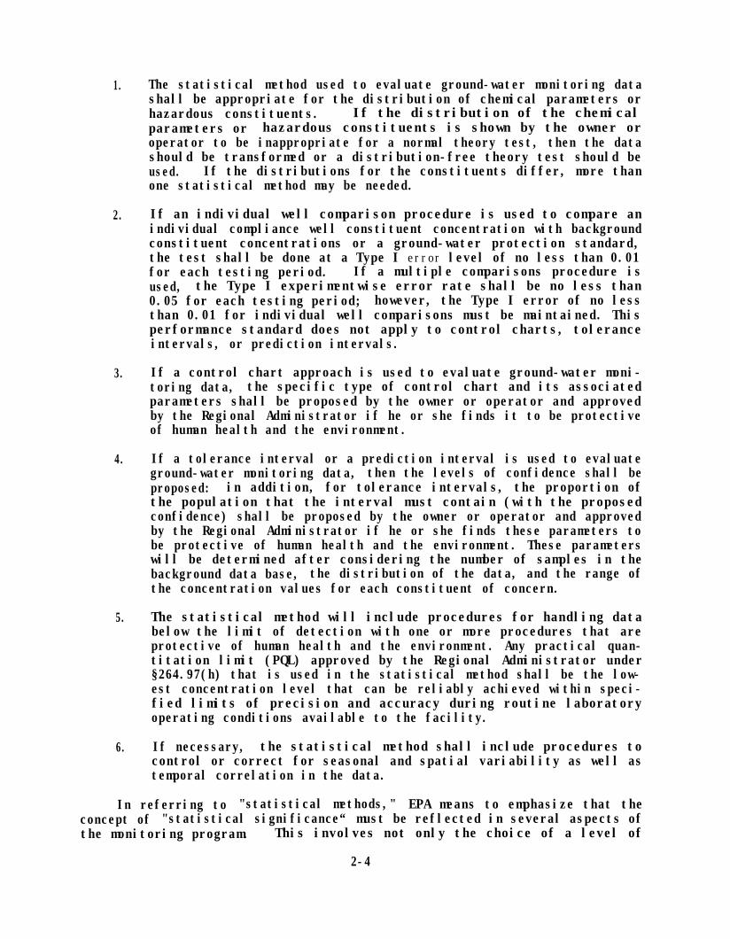
The statistical method used to evaluate ground-water monitoring datashall be appropriate for the distribution of chemical parameters orhazardous constituents. If the distribution of the chemicalparameters or hazardous constituents is shown by the owner oroperator to be inappropriate for a normal theory test, then the datashould be transformed or a distribution-free theory test should beused. If the distributions for the constituents differ, more thanone statistical method may be needed.

If an individual well comparison procedure is used to compare anindividual compliance well constituent concentration with backgroundconstituent concentrations or a ground-water protection standard,the test shall be done at a Type I error level of no less than 0.01for each testing period. If a multiple comparisons procedure isused, the Type I experimentwise error rate shall be no less than0.05 for each testing period; however, the Type I error of no lessthan 0.01 for individual well comparisons must be maintained. Thisperformance standard does not apply to control charts, toleranceintervals, or prediction intervals.

3. If a control chart approach is used to evaluate ground-water moni-toring data, the specific type of control chart and its associatedparameters shall be proposed by the owner or operator and approvedby the Regional Administrator if he or she finds it to be protectiveof human health and the environment.

4. If a tolerance interval or a prediction interval is used to evaluateground-water monitoring data, then the levels of confidence shall beproposed: in addition, for tolerance intervals, the proportion ofthe population that the interval must contain (with the proposedconfidence) shall be proposed by the owner or operator and approvedby the Regional Administrator if he or she finds these parameters tobe protective of human health and the environment. These parameterswill be determined after considering the number of samples in thebackground data base, the distribution of the data, and the range ofthe concentration values for each constituent of concern.

5. The statistical method will include procedures for handling databelow the limit of detection with one or more procedures that areprotective of human health and the environment. Any practical quan-titation limit (PQL) approved by the Regional Administrator under§264.97(h) that is used in the statistical method shall be the low-est concentration level that can be reliably achieved within speci-fied limits of precision and accuracy during routine laboratoryoperating conditions available to the facility.

6. If necessary, the statistical method shall include procedures tocontrol or correct for seasonal and spatial variability as well astemporal correlation in the data.

In referring to "statistical methods," EPA means to emphasize that theconcept of "statistical significance“ must be reflected in several aspects ofthe monitoring program. This involves not only the choice of a level of

2-4

significance, but also the choice of a statistical test, the sampling require-ments, the number of samples, and the frequency of sampling. Since all ofthese parameters interact to determine the ability of the procedure to detectcontamination, the statistical methods, like a comprehensive ground-watermonitoring program, must be evaluated in their entirety, not by individualcomponents. Thus a systems approach to ground-water monitoring is endorsed.

The second performance standard requires further comment. For individualwell comparisons in which an individual compliance well is compared to back-ground, the Type I error level shall be no less than 1% (0.01) for each test-ing period. In other words, the probability of the test resulting in a falsepositive is no less than 1 in 100. EPA believes that this significance levelis sufficient in limiting the false positive rate while at the same time con-trolling the false negative (missed detection) rate.

Owners and operators of facilities that have an extensive network ofground-water monitoring wells may find it more practical to use a multiplewell comparisons procedure. Multiple comparisons procedures control theexperimentwise error rate for comparisons involving multiple upgradient anddowngradient wells. If this method is used, the Type I experimentwise errorrate for each constituent shall be no less than 5% (0.05) for each testingperiod.

In using a multiple well comparisons procedure, if the owner or operatorchooses to use a t-statistic rather than an F-statistic, the individual wellType I error level must be maintained at no less than 1% (0.01). Thisprovision should be considered if a facility owner or operator wishes to use aprocedure that distributes the risk of a false positive evenly throughout allmonitoring wells (e.g., Bonferroni t-test).

Setting these levels of significance at 1% and 5%, respectively, raisesan important question in how the false positive rate will be controlled atfacilities with a large number of ground-water monitoring wells and monitoringconstituents. The Agency set these levels of significance on the basis of asingle testing period and not on the entire operating life of the facility.Further, large facilities can reduce the false positive rate by implementing aunit-specific monitoring approach. Data from uncontaminated upgradient wellscan be pooled and treated as one group. This will not only reduce the numberof comparisons in a multiple well comparisons procedure but will also takeinto account spatial heterogeneities that may affect background ground-waterquality. If the overall F-test is significant, then testing of the contrastsbetween the mean of each compliance well concentration and the mean backgroundconcentration must be performed for each constituent. This will identify themonitoring wells that are out of compliance. The Type I error level for theindividual comparisons shall be no less than 0.01. Nonetheless, it is evidentthat facilities with an extensive number of ground-water monitoring wellswhich are monitored for many constituents may still generate a large number ofcomparisons during each testing period.

In these particular situations, a determination of whether a release froma facility has occurred may require the Regional Administrator to evaluate thesite hydrogeology, geochemistry, climatic factors, and other environmentalparameters to determine if a statistically significant result is indicative of

2-5

an actual release from the facility. In making this determination, theRegional Administrator may note the relative magnitude of the concentration ofthe constituent(s). If the exceedance is based on an observed compliance wellvalue that is the same relative magnitude as the PQL (practical quantitationlimit) or the background concentration level, then a false positive may haveoccurred, and further sampling and testing may be appropriate. If, however,the background concentration level or an action level is substantiallyexceeded, then the exceedance is more likely to be indicative of a releasefrom the facility.

2.4 BASIC STATISTICAL METHODS AND SAMPLING PROCEDURES

The October 11, 1988 rule specifies five types of statistical methods todetect contamination in ground water. EPA believes that at least one of thesetypes of procedures will be appropriate for virtually all facilities. Toaddress situations where these methods may not be appropriate, EPA hasincluded a provision for the owner or operator to select an alternate methodwhich is subject to approval by the Regional Administrator.

2.4.1 The Five Statistical Methods Outlined in the October 11, 1988 FinalRule

1.

2.

3.

4.

5.

A parametric analysis of variance (ANOVA) followed by multiple com-parison procedures to identify specific sources of difference. Theprocedures will include estimation and testing of the contrastsbetween the mean of each compliance well and the background mean foreach constituent.

An analysis of variance (ANOVA) based on ranks followed by multiplecomparison procedures to identify specific sources of difference.The procedure will include estimation and testing of the contrastsbetween the median of each compliance well and the median backgroundlevels for each constituent.

A procedure in which a tolerance interval or a prediction intervalfor each constituent is established from the background data, andthe level of each constituent in each compliance well is compared toits upper tolerance or prediction limit.

A control chart approach which will give control limits for eachconstituent. If any compliance well has a value or a sequence ofvalues that lie outside the control limits for that constituent, itmay constitute statistically significant evidence of contamination.

Another statistical method submitted by the owner or operator andapproved by the Regional Administrator.

A summary of these statistical methods and their applicability is pre-sented in Table 2-1. The table lists types of comparisons and the recommendedprocedure and refers the reader to the appropriate sections where a discussionand example can be found.

2-6

TABLE 2-1. SUMMARY OF STATISTICAL METHODS

SUMMARY OF STATISTICAL METHODSSECTION OF

COMPOUND TYPE OF COMPARISON RECOMMENDED METHOD GUIDANCE

I DOCUMENT

ANYCOMPOUND

IN

BACKGROUND VSANOVA 5.2

COMPLIANCE WELLTOLERANCE LIMITS 5.3

PREDICTION INTERVALS 5.4

BACKGROUND INTRA-WELL CONTROL CHARTS 7

ACL/MCL FIXED STANDARDCONFIDENCE INTERVALS 6.2.1

SPECIFIC TOLERANCE LIMITS 6.2.2

S Y N T H E T I C M A N Y N O N D E T E C T S SEE BELOW DETECTIONIN DATA SET LIMIT TABLE 8-l 8.1

2-7

EPA is specifying multiple statistical methods and sampling proceduresand has allowed for alternatives because no one method or procedure is appro-priate for all circumstances. EPA believes that the suggested methods andprocedures are appropriate for the site-specific design and analysis of datafrom ground-water monitoring systems and that they can account for more of thesite-specific factors that Cochran's Approximation to the Behrens-FisherStudent's t-test (CABF) and the accompanying sampling procedures in the pastregulations. The statistical methods specified here address the multiplecomparison problems and provide for documenting and accounting for sources ofnatural variation. EPA believes that the specified statistical methods andprocedures consider and control for natural temporal and spatial variation.

2.4.2 Site-Specific Considerations for Sampling

The decision on the number of wells needed in a monitoring system will bemade on a site-specific basis by the Regional Administrator and will considerthe statistical method being used, the site hydrogeology, the fate and trans-port characteristics of potential contaminants, and the sampling procedure.The number of wells must be sufficient to ensure a high probability of detect-ing contamination when it is present. To determine which sampling procedureshould be used, the owner or operator shall consider existing data and sitecharacteristics, including the possibility of trends and seasonality. Thesesampling procedures are:

1. Obtain a sequence of at least four samples taken at an interval thatensures, to the greatest extent technically feasible, that an inde-pendent sample is obtained, by reference to the uppermost aquifer'seffective porosity, hydraulic conductivity, and hydraulic gradient,and the fate and transport characteristics of potential contami-nants. The sampling interval that is proposed must be approved bythe Regional Administrator.

2. An alternate sampling procedure proposed by the owner or operatorand approved by the Regional Administrator if he or she finds it tobe protective of human health and the environment.

EPA believes that the above sampling procedures will allow the use ofstatistical methods that will accurately detect contamination. These samplingprocedures may be used to replace the sampling method present in the formerSubpart F regulations. Rather than taking a single ground-water sample anddividing it into four replicate samples, a sequence of at least four samplestaken at intervals far enough apart in time (daily, weekly, or monthly,depending on rates of ground-water flow and contaminant fate and transportcharacteristics) will help ensure the sampling of a discrete portion (i.e., anindependent sample) of ground water. In hydrogeologic environments where theground-water velocity prohibits one from obtaining four independent samples ona semiannual basis, an alternate sampling procedure approved by the RegionalAdministrator may be utilized 140 CFR §264.97(g)(l) and (2)].

The Regional Administrator shall approve an appropriate sampling proce-dure and interval submitted by the owner or operator after considering theeffective porosity, hydraulic conductivity, and hydraulic gradient in theuppermost aquifer under the waste management area, and the fate and transport

2-8

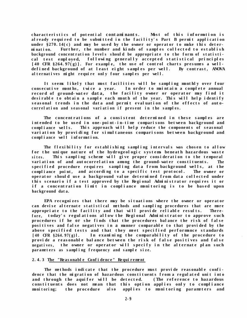
characteristics of potential contaminants. Most of this information isalready required to be submitted in the facility's Part B permit applicationunder §270.14(c) and may be used by the owner or operator to make this deter-mination. Further, the number and kinds of samples collected to establishbackground concentration levels should be appropriate to the form of statisti-cal test employed, following generally accepted statistical principles[40 CFR §264.97(g)]. For example, the use of control charts presumes a well-defined background of at least eight samples per well. By contrast, ANOVAalternatives might require only four samples per well.

It seems likely that most facilities will be sampling monthly over fourconsecutive months, twice a year. In order to maintain a complete annualrecord of ground-water data, the facility owner or operator may find itdesirable to obtain a sample each month of the year. This will help identifyseasonal trends in the data and permit evaluation of the effects of auto-correlation and seasonal variation if present in the samples.

The concentrations of a consistent determined in these samples areintended to be used in one-point-in-time comparisons between background andcompliance wells. This approach will help reduce the components of seasonalvariation by providing for simultaneous comparisons between background andcompliance well information.

The flexibility for establishing sampling intervals was chosen to allowfor the unique nature of the hydrogeologic systems beneath hazardous wastesites. This sampling scheme will give proper consideration to the temporalvariation of and autocorrelation among the ground-water constituents. Thespecified procedure requires sampling data from background wells, at thecompliance point, and according to a specific test protocol. The owner oroperator should use a background value determined from data collected underthis scenario if a test approved by the Regional Administrator requires it orif a concentration limit in compliance monitoring is to be based uponbackground data.

EPA recognizes that there may be situations where the owner or operatorcan devise alternate statistical methods and sampling procedures that are moreappropriate to the facility and that will provide reliable results. There-fore, today's regulations allow the Regional Administrator to approve suchprocedures if he or she finds that the procedures balance the risk of falsepositives and false negatives in a manner comparable to that provided by theabove specified tests and that they meet specified performance standards[40 CFR §264.97(g)l. In examining the comparability of the procedure toprovide a reasonable balance between the risk of false positives and falsenegatives, the owner or operator will specify in the alternate plan suchparameters as sampling frequency and sample size.

.

2.4.3 The "Reasonable Confidence" Requirement

The methods indicate that the procedure must provide reasonable confi-dence that the migration of hazardous constituents from a regulated unit intoand through the aquifer will be detected. (The reference to hazardousconstituents does not mean that this option applies only to compliancemonitoring; the procedure also applies to monitoring parameters and

2-9

constituents in the detection monitoring program since they are surrogatesindicating the presence of hazardous constituents.) The protocols for thespecific tests, however, will be used as general benchmark to define"reasonable confidence" in the proposed procedure. If the owner or operatorshows that his or her suggested test is comparable in its results to one ofthe specified tests, then it is likely to be acceptable under the 'reasonableconfidence" test. There may be situations, however, where it will bedifficult to directly compare the performance of an alternate test to theprotocols for the specified tests. In such cases the alternate test will haveto be evaluated on its own merits.

2.4.4 Implementation

Owners and operators currently operating under a RCRA permit andemploying the CABF procedure may change this procedure to a more appropriateprocedure at the time of State or Regional permit review and update. Ofcourse, these owners and operators may also apply for a permit modificationunder § 270.41(a)(3). This change is considered a Class 1 permit modifica-tion. Class 1 permit modifications are technical in nature and generally oflimited interest to the public. Class 1 modifications may be made with priorapproval from the Director. The reader is referred to 53 FR 37912,September 28, 1988 for more details about the permit modification process.

Under appropriate circumstances, the owner or operator may wish tocontinue using the CABF procedure. This would involve a facility that hascomparably few monitoring wells (e.g., fewer than five) and monitors for onlya limited number of chemical parameters and hazardous constituents (e.g.,fewer than four). In this case, fewer than 20 comparisons would be made eachtesting period, and performing the CABF procedure at the 0.05 level of sig-nificance may result in no more than one false positive each testing period.The owner or operator should consider a similar evaluation when deciding theadequacy of the CABF procedure for his or her facility. Likewise, the owneror operator should also continually update the background concentrations inupgradient monitoring wells and simultaneously compare aggregate upgradientwell data (background wells) to downgradient well data (compliance wells).This practice will help reduce the component of temporal variability associ-ated with the CABF procedure. Further, efforts should be made to obtainindependent samples from the monitoring wells. Section 3 of the guidanceaddresses how one might accomplish this task. If situations permit, thereplicate sampling procedure should be avoided. Replicate samples provideinformation about analytical variability and accuracy. The goal of all RCRAground-water sampling programs should be to provide data about the hydro-geochemical variability in the aquifers below the hazardous waste facility.Obtaining independent samples when possible will help reduce the effects ofautocorrelation.

In all cases any statistical method or sampling procedure must beapproved by the Regional Administrator or State Director. Changing from onestatistical method or sampling procedure to another may be done at the time ofRegional or State permit review and update, or at any time a Class 1 permitmodification is approved (see 53 RF 37912, September 28, 1988).

2-10

SECTION 3

CHOOSING A SAMPLING INTERVAL

This section discusses the important hydrogeologic parameters to considerwhen choosing a sampling interval. The Darcy equation is used to determinethe horizontal component of the average linear velocity of ground water forconfined, semiconfined, and unconfined aquifers. This value provides a goodestimate of time of travel for most soluble constituents in ground water, andcan be used to determine a sampling interval. Example calculations are pro-vided at the end of the section to further assist the reader. Alternativemethods must be employed to determine a sampling interval in hydrogeologicenvironments where Darcy's law is invalid. Karst, cavernous basalt, fracturedrocks, and other "pseudo karst" terranes usually require specialized monitor-ing approaches.

Section 264.97(g) of 40 CFR Part 264 Subpart F provides the owner oroperator of a RCRA facility with a flexible sampling schedule that will allowhim or her to choose a sampling procedure that will reflect site-specific con-cerns. This section specifies that the owner or operator shall, on a semi-annual basis, obtain a sequence of at least four samples from each well, basedon an interval that is determined after evaluating the uppermost aquifer'seffective porosity, hydraulic conductivity, and hydraulic gradient, and thefate and transport characteristics of potential contaminants. The intent ofthis provision is to set a sampling frequency that allows sufficient time topass between sampling events to ensure, to the greatest extent technicallyfeasible, that an independent ground-water sample is taken from each well.For further information on ground-water sampling, refer to the EPA "PracticalGuide for Ground-Water Sampling," Barcelona et al., 1985.

The sampling frequency of the four semiannual sampling events required inPart 264 Subpart F can be based on estimates using the average linear velocityof ground water. Two forms of the Darcy equation stated below relate ground-water velocity (V) to effective porosity (Ne), hydraulic gradient (i), andhydraulic conductivity (K):

Vh=(Kh*i)/Ne and Vv,=(Kv,*i)/Ne

where Vh and Vv are the horizontal and vertical components of the averagelinear velocity of ground water, respectively; Kh and Kv are the horizontaland vertical components of hydraulic conductivity; i is the head gradient; andNe is the effective porosity. In applying these equations to ground-watermonitoring, the horizontal Component of the average linear Velocity (Vh) canbe used to determine an appropriate sampling interval. Usually, field

3-1

investigations will yield bulk values for hydraulic conductivity. In mostcases, the bulk hydraulic conductivity determined by a pump test, tracer test,or a slug test will be sufficient for these calculations. The vertical com-ponent of the average linear velocity of ground water (VV,) may be consideredin estimating flow velocities in areas with significant components of verticalvelocity such as recharge and discharge zones.

To apply the Darcy equation to ground-water monitoring, one needs todetermine the parameters K, i, and Ne. The hydraulic conductivity, K, is thevolume of water at the existing kinematic viscosity that will move in unittime under a unit hydraulic gradient through a unit area measured at rightangles to the direction of flow. The reference to "existing kinematic vis-cosity" relates to the fact that hydraulic conductivity is not only determinedby the media (aquifer), but also by fluid properties (ground water or poten-tial contaminants). Thus, it is possible to have several hydraulic conduc-tivity values for many different chemical substances that are present in thesame aquifer. In either case it is advisable to use the greatest value forvelocity that is calculated using the Oarcy equation to determine samplingintervals. This will provide for the earliest detection of a leak from ahazardous waste facility and expeditious remedial action procedures. A rangeof hydraulic conductivities (the transmitted fluid is water) for various aqui-fer materials is given in Figures 3-1 and 3-2. The conductivities are givenin several units. Figure 3-3 lists conversion factors to change between vari-ous permeability and hydraulic conductivity units.

The hydraulic gradient, i, is the change in hydraulic head per unit ofdistance in a given direction. It can be determined by dividing the differ-ence in head between two points on a potentiometric surface map by theorthogonal distance between those two points (see example calculation). Waterlevel measurements are normally used to determine the natural hydraulic gradi-ent at a facility. However, the effects of mounding in the event of a leakfrom a waste disposal facility may produce a steeper local hydraulic gradientin the vicinity of the monitoring well. These local changes in hydraulicgradient should be accounted for in the velocity calculations.

The effective porosity, Ne, is the ratio, usually expressed as a per-centage, of the total volume of voids available for fluid transmission to thetotal volume of the porous medium dewatered. It can be estimated during apump test by dividing the volume of water removed from an aquifer by the totalvolume of aquifer dewatered (see example calculation). Table 3-l presentsapproximate effective porosity values for a variety of aquifer material-s. Incases where the effective porosity is unknown, specific yield may be substi-tuted into the equation. Specific yields of selected rock units are given inTable 3-2. In the absence of measured values, drainable porosity is oftenused to approximate effective porosity. Figure 3-4 illustrates representativevalues of drainable porosity and total porosity as a function of aquiferparticle size. If available, field measurements of effective porosity arepreferred.

3-2

IGNEOUS A N D M E T A M O R P H I C R O C K S

U n f r a c r u r e d F r a c t u r e dBASALT

U n f r a c t u r e d Fractured L a v a f l o w

SANDSTONEFractured S e m i c o n s o l i d a t e d

S H A L E

U n f r a c t u r e d FracturedCARBONATE ROCKS

Fractured C o v e r n o u s

C L A Y SILT, LOESS

SILTY SAND

GLACIAL TILL

C L E A N S A N D

F i n e C o a r s eGRAVEL

108 10-7 10-6 10-5 l0-4 l0-3 10-2 1 0 - 1 1 1 0 I O 2 I 0 3 1 0 4

m / d a y

1 0 71 0 6 1 0 - 5 1 0 4 I O - 3 l 0 - 2 l 0 - 1 1 10 10 2 IO 3 IO 4 10 5

f t / d a y

1 0 - 71 0 - 6

1 0 - 5 l 0 - 41 O - 3

1 0 21 0 1

1 10 IO 2 10 3 IO 4 10 5

g a l / d a y - f t 2

Source: Heath, R. C. 1983. Basic Ground-Water Hydrology. U.S. GeologicalSurvey Water Supply Paper, 2220, 84 pp.

Figure 3-1. Hydraulic conductivity of selected rocks.

3 - 3

*To obtain k in ftz, multiply k in cm2 by 1.08 x 10-3.

Source: Freeze, R. A., and J. A. Cherry. 1979. Ground Water. PrenticeHall, Inc., Englewood Cliffs, New Jersey. p. 29.

Figure 3-3. Conversion factors for permeability andhydraulic conductivity units.

3-4

TABLE 3-I. DEFAULT VALUES FOR EFFECTIVE POROSITY (Ne) FOR USEIN TIME OF TRAVEL (TOT) ANALYSES

Soil textural classesEffective porosityof saturationa

Unified soil classification system

GS, GP, GM, GC, SW, SP, SM, SC 0.20(20%)

ML, MH 0.15(15%)

CL, OL, CH, OH, PT 0.01(1%)b

USDA soil textural classes

Clays, silty clays, sandy clays 0.01(1%)b

Silts, silt loams, silty clay loams 0.10(10%)

All others 0.20(20%)

Rock units (all)

Porous media (nonfractured rockssuch as sandstone and some carbonates)

0.15(15%)

Fractured rocks (most carbonates, 0.0001shales, granites, etc.) (0.01%)

Source: Barari, A., and L. S. Hedges. 1985. Movement of Waterin Glacial Till. Proceedings of the 17th International Congress of theInternational Association of Hydrogeologists, pp. 129-134.a These values are estimates and there may be differences between

similar units. For example, recent studies indicate thatweathered and unweathered glacial till may have markedly dif-ferent effective porosities (Barari and Hedges, 1985; Bradburyet al., 1985).

b Assumes de minimus secondary porosity. If fractures or soilstructure are present, effective porosity should be 0.001(0.1%).

3-5

TABLE 3-2. SPECIFIC YIELD VALUES FORSELECTED ROCK TYPES

Rock type Specific yield (%)

ClaySandGravelLimestoneSandstone (semiconsolidated)GraniteBasalt (young)

22191860.098

Source: Heath, R. C. 1983. Basic Ground-WaterHydrology. U.S. Geological Survey, Water SupplyPaper 2220, 84 pp.

3-6

50

45

40

35

30

- 2S=II'" 20;

Q,.

15

10

S

0

,",/

'ii Ii

-='tl > > Ii Ii=: ... ...

=Q ;: c3 c3 > >;;; > ... Ii ... ...;e ...'" -= '" '" :> Ot & ...U '" '" > '" E E- ; ;;; c: ;;

i :; :I; e; ;, .. ..~

... ... ... 'ii ~ ::l ... '" 32>- ~ ~ . ~ ;; :> S - ;0 :i 5'"

~ ii.. j :II <3... 0 c

C ... ... :E U r,; ... :E :E (.,l (.,l a:I

1/16 1/18 1/4 1/2 1 2 4 8 16 32 64 128 256

MaXImum 10% grain Size. millimeters(Th. i,.,n ./Z. In wIt/CII. til. cumul.rll'. rorM. O.gmnmi "111m til. co.n••t m.r.,,-'.r.Kllft 10~ of rfl. tor.' •.",",•. J

Source: Todd, O. K. 1980. Ground Water Hydrology. JohnWiley and Sons, New York. 534 pp.

Figure 3-4. Total porosity and drainable porosity fortypical geologic materials.

3-7

Once the values for K, i, and Ne are determined, the horizontal componentof the average linear velocity of ground water can be calculated. Using theDarcy equation, we can determine the time required for ground water to passthrough the complete monitoring well diameter by dividing the monitoring welldiameter by the horizontal component of the average linear velocity of groundwater. (If considerable exchange of water occurs during well purging, thediameter of the filter pack may be used rather than the monitoring well diam-eter.) This value will represent the minimum time interval required betweensampling events that will yield an independent ground-water sample. (Three-dimensional mixing of ground water in the vicinity of the monitoring well willoccur when the well is purged before sampling, which is one reason why thismethod only provides an estimation of travel time).

In determining these sampling intervals, one should note that many chemi-cal compounds will not travel at the same velocity as ground water. Chemicalcharacteristics such as adsorptive potential, specific gravity, and molecularsize will influence the way chemicals travel in the subsurface. Large mole-cules, for example, will tend to travel slower than the average linear veloc-ity of ground water because of matrix interactions. Compounds that exhibit astrong adsorptive potential will undergo a similar fate that will dramaticallychange time of travel predictions using the Darcy equation. In some caseschemical interaction with the matrix material will alter the matrix structureand its associated hydraulic conductivity that may result in an increase incontaminant mobility. This effect has been observed with certain organicsolvents in clay units (see Brown and Andersen, 1981). Contaminant fate andtransport models may be useful in determining the influence of these effectson movement in the subsurface. A variety of these models are available on thecommercial market for private use.

3.1 EXAMPLE CALCULATIONS

EXAMPLE CALCULATION NO. 1: DETERMINING THE EFFECTIVE POROSITY (He)

The effective porosity, Ne, expressed in %, can be determined during apump test using the following method:

Ne = 100% x volume of water removed/volume of aquifer dewatered

Based on a pumping rate of the pump of 50 gal/min and a pumpingduration of 30 min, compute the volume of water removed as:

50 gal/min x 30 min = 1,500 gal

ed, use the formula:. To calculate the volume of aquifer dewater

where r is the radius (ft) of area affected by pump ing and h (ft) is the dropin the water level. If, for example, h = 3 ft and r = 18 ft, then:

V = (l/3)*3.14*182*3 = 1,018 ft3

3-8

Next, converting ft3 of water to gallons of water,

V = (1,018 ft3)(7.48 gal/ft3) = 7,615 gal

Substituting the two volumes in the equation for the effectiveporosity, obtain

Ne = 100% x 1,500/7,615 = 19.7%

EXAMPLE CALCULATION NO. 2: DETERMINING THE HYDRAULIC GRADIENT (i)

Using the values given in Figure 3-3, obtain

Figure 3-5. Potentiometric surface map for computationof hydraulic gradient.

This method provides only a very general estimate of the naturalhydraulic gradient that exists in the vicinity of the two piezometers.Chemical gradients are known to exist and may override the effects of thehydraulic gradient. A detailed study of the effects of multiple chemicalcontaminants may be necessary to determine the actual average linear velocity(horizontal component) of ground water in the vicinity of the monitoringwells.

3-9

EXAMPLE CALCULATION NO. 3: DETERMINING THE HORIZONTAL COMPONENT OF THEAVERAGE LINEAR VELOCITY OF GROUND MATER (Vh)

A land disposal facility has ground-water monitoring wells that arescreened in an unconfined silty sand aquifer. Slug tests, pump tests, andtracer tests conducted during a hydrogeologic site investigation have revealedthat the aquifer has a horizontal hydraulic conductivity (Kh) of 15 ft/day andan effective porosity (Ne) of 15%. Using a potentiometric map (as inexample 2), the hydraulic gradient (i) has been determined to be 0.003 ft/ft.

To estimate the minimum time interval between sampling events that willallow one to obtain an independent sample of ground water proceed as follows.

Calculate the horizontal component of the average linear velocity ofground water (Vh) using the Darcy equation, Vh = (Kh*i)/Ne.

With Kh = 15 ft/day,Ne = 15%, and

i = 0.003 ft/ft, calculate

Vh = (15)(0.003)/(15%) = 0.3 ft/day, or equivalently

vh = (0.3 ft/day)(l2 in/ft) = 3.6 in/day

Discussion: The horizontal component of the average linear velocity ofground water, Vh, has been calculated and is equal to 3.6 in/day. Monitoringwell diameters at this particular facility are 4 in. We can determine theminimum time interval between sampling events that will allow one to obtain anindependent sample of ground water by dividing the monitoring well diameter bythe horizontal component of the average linear velocity of ground water:

Minimum time interval = (4 in)/(3.6 in/day) = 1.1 days

Based on the above calculations, the owner or operator could sample everyother day. However, because the velocity can vary with recharge rates sea-sonally, a weekly sampling interval would be advised.

Suggested Sampling Interval

Date Obtain Sample No.

June 1 1June 8 2June 15 3June 22 4

Table 3-3 gives some results for common situations.

3-10

TABLE 3-3. DETERMINING A SAMPLING INTERVAL

DETERMINING A SAMPLING INTERVAL

UNIT Kh, (ftday)

GRAVEL 1 0 4

SAND 102

SILTY SAND 10

TILL I0 - 3

SS (SEMICON) 1

BASALT 10 - 1

Ne (%) vh (in/mo

19 9 . 6 x l 0 4

22 8.3 x l 0 2

14 1.3x l 0 2

2 9.1 x 10-2

6 30

8 2.28

SAMPLING INTERVAL

DAILY

DAILY

WEEKLY

MONTHLY *

WEEKLY

MONTHLY *

The horizontal component of the average linear velocities is based ona hydraulic gradient, i, of 0.005 ft/ft.

?? Use a Monthly sampling interval or an alternate sampling procedure.

3.2 FLOW THROUGH KARST AND “PSEUDO-KARST” TERRANES

The Darcy equation is not valid in turbulent and nonlinear laminar flowregimes. Examples of these particular hydrogeological environments includekarst and "pseudo-karst" (e.g., cavernous basalts and extensively fracturedrocks) terranes. Specialized methods have been investigated by Quinlan (1989)for developing alternative monitoring procedures for karst and "pseudo-karst"terranes. Dye tracing as described by Quinlan (1989) and Mull et al. (1988)is useful for identifying flow paths and travel times in karst and "pseudo-karst" terranes. Conventional ground-water monitoring wells in theseenvironments are often of little value in designing an effective monitoringsystem. Field investigations are necessary to locate seeps and springs, whichmay serve as better "monitoring wells" for identifying releases of hazardousconstituents into ground water and surface water.

3-11

SECTION 4

CHOOSING A STATISTICAL METHOD

This section discusses the choice of an appropriate statistical method.Section 4.1 includes a flowchart to guide this selection. Section 4.2 containsprocedures to test the distributional assumptions of statistical methods andSection 4.3 has procedures to test specifically for equality of variances.

The choice of an appropriate statistical test depends on the type of mon-itoring and the nature of the data. The proportion of values in the data setthat are below detection is one important consideration. If most of thevalues are below detection, a test of proportions is suggested.

One set of statistical procedures is suggested when the monitoring con-sists of comparisons of water sample data from the background (hydraulicallyupgradient) well with the sample data from compliance (hydraulically down-gradient) wells. The recommended approach is analysis of variance (ANOVA).Also, for a facility with limited amounts of data, it is advisable to ini-tially use the ANOVA method of data evaluation, and later, when sufficientamounts of data are collected, to change to a tolerance interval or a controlchart approach for each compliance well. However, alternate approaches areal lowed. These include adjustments for seasonality, use of tolerance inter-vals, and use of prediction intervals. These methods are discussed in Sec-tion 5.

When the monitoring objective is to compare the concentration of a haz-ardous constituent to a fixed level such as a maximum concentration limit(MCL), a different type of approach is needed. This type of comparison com-monly serves as a basis of compliance monitoring. Control charts may be used,as may tolerance or confidence intervals. Methods for comparison with a fixedlevel are presented in Section 6.

When a long history of data from each well is available, intra-well com-parisons are appropriate. That is, the data from a single uncontaminated wellare compared over time to detect shifts in concentration, or gradual trends inconcentration that may indicate contamination. Methods for this situation arepresented in Section 7.

4.1 FLOWCHARTS--OVERVIEW AND USE

The selection and use of a statistical procedure for ground-water moni-toring is a detailed process. Because a single flowchart would become toocomplicated for easy use, a series of flowcharts has been developed. Theseflowcharts are found at the beginning of each section and are intended to

4-1

guide the user in the selection and use of procedures in that section. Themore detailed flowcharts can be thought of as attaching to the general flow-charts at the indicated points.

Three general types of statistical procedures are presented in the flow-chart overview (Figure 4-l): (1) background well to compliance well datacomparisons; (2) comparison of compliance well data with a constant limit suchas an alternate concentration limit (ACL) or a maximum concentration limit(MCL); and (3) intra-well comparisons. The first question to be asked indetermining the appropriate statistical procedure is the type of monitoringprogram specified in facility permit. The type of monitoring program maydetermine if the appropriate comparison is among wells, comparison of down-gradient well data to a constant, intra-well comparisons, or a special case.

If the facility is in detection monitoring, the appropriate comparison isbetween wells that are hydraulically upgradient from the facility and thosethat are hydraulically downgradient. The statistical procedures for this typeof monitoring are presented in Section 5. In detection monitoring, it islikely that many of the monitored constituents may result in few quantifiedresults (i.e., much of the data are below the limit of analytical detection).If this is the case, then the test of proportions (Section 8.1.3) may be rec-ommended. If the constituent occurs in measurable concentrations in back-ground, then analysis of variance (Section 5.2) is recommended. This methodof analysis is preferred when the data lack sufficient quantity to allow forthe use of tolerance intervals or control charts.

If the facility is in compliance monitoring, the permit will specify thetype of compliance limit. If the compliance limit is determined from thebackground, the statistical method is chosen from those that compare back-ground well to compliance well data. Statistical methods for this case arepresented in Section 5. The preferred method is the appropriate analysis ofvariance method in Section 5.2, or if sufficient data permit, tolerance inter-vals or control charts. The flow chart in Section 5 aids in determining whichmethod is applicable.

If a facility in compliance monitoring has a constant maximum concentra-tion limit (MCL) or alternate concentration limit (ACL) specified, then theappropriate comparison is with a constant. Methods for comparison with MCLsor ACLs are presented in Section 6, which contains a flow chart to aid indetermining which method to use.

Finally, when more than one year of data have been collected from eachwell, the facility owner or operator may find it useful to perform intra-wellcomparisons over time to supplement the other methods. This is not a regula-tory requirement, but it could provide the facility owner or operator withinformation about the site hydrogeology. This method of analysis may be usedwhen sufficient data from an individual uncontaminated well exist and the dataallow for the identification of trends. A recommended control chart procedure(Starks, 1988) suggests that a minimum background sample of eight observationsis needed. Thus an intra-well control chart approach could begin after thefirst complete year of data collection. These methods are presented inSection 7.

4-2

FLOWCHART OVERVIEW

Background

Figure 4-1. Flowchart overview.

4-3

4.2 CHECKING DISTRIBUTIONAL ASSUMPTIONS

The purpose of this section is to provide users with methods to check thedistributional assumptions of the statistical procedures recommended forground-water monitoring. It is emphasized that one need not do an extensivestudy of the distribution of the data unless a nonparametric method of analy-sis is used to evaluate the data. If the owner or operator wishes to trans-form the data in lieu of using a nonparametric method, it must first be shownthat the untransformed data are inappropriate for a normal theory test.Similarly, if the owner or operator wishes to use nonparametric methods, he orshe must demonstrate that the data do violate normality assumptions.

EPA has adopted this approach because most of the statistical proceduresthat meet the criteria set forth in the regulations are robust with respect todepartures from many of the normal distributional assumptions. That is, onlyextreme violations of assumptions will result in an incorrect outcome of astatistical test. Moreover, it is only in situations where it is unclearwhether contamination is present that departures from assumptions will alterthe outcome of a statistical test. EPA therefore believes that it is protec-tive of the environment to adopt the approach of not requiring testing ofassumptions of a normal distribution on a wide scale.

It should be noted that the normal distributional assumptions forstatistical procedures apply to the errors of the observations. Applicationof the distributional tests to the observations themselves may lead to theconclusion that the distribution does not fit the observations. In some casesthis lack of fit may be due to differences in means for the different wells orsome other cause. The tests far distributional assumptions are best appliedto the residuals from a statistical analysis. A residual is the differencebetween the original observation and the value predicted by a model. Forexample, in analysis of variance, the predicted values are the group means andthe residual is the difference between each observation and its group mean.

If the conclusion from testing the assumptions is that the assumptionsare not adequately met, then a transformation of the data may be used or anonparametric statistical procedure selected. Many types of concentrationdata have been reported in the literature to be adequately described by a log-normal distribution. That is, the natural logarithm of the original observa-tions has been found to follow the normal distribution. Consequently, if thenormal distributional assumptions are found to be violated for the originaldata, a transformation by taking the natural logarithm of each observation issuggested. This assumes that the data are all positive. If the log trans-formation does not adequately normalize the data or stabilize the variance,one should use a nonparametric procedure or seek the consultation of a profes-sional statistician to determine an appropriate statistical procedure.

The following sections present four selected approaches to check fornormality. The first option refers to literature citation, the other threeare statistical procedures. The choice is left to the user. The availabilityof statistical software and the user's familiarity with it will be a factor inthe choice of a method. The coefficient of variation method, for example,requires only the computation of the mean and standard deviation of the data.

4-4

Plotting on probability paper can be done by hand but becomes tedious withmany data sets. However, the commercial Statistical Analysis System (SAS)software package provides a computerized version of a probability plot in itsPROC UNIVARIATE procedure. SYSTAT, a package for PCs also has a probabilityplot procedure. The chi-squared test is not readily available through commer-cial software but can be programmed on a PC (for example in LOTUS l-2-3) or inany other (statistical) software language with which the user is familiar.The amount of data available will also influence the choice. All tests ofdistributional assumptions require a fairly large sample size to detectmoderate to small deviations from normality. The chi-squared test requires aminimum of 20 samples for a reasonable test.

Other statistical procedures are available for checking distributionalassumptions. The more advanced user is referred to the Kolmogorov-Smirnovtest (see, for example, Lindgren, 1976) which is used to test the hypothesisthat data come from a specific (that is, completely specified) distribution.The normal distribution assumption can thus be tested for. A minimum samplesize of 50 is recommended for using this test.

A modification to the Kolmogorov-Smirnov test has been developed byLilliefors who uses the sample mean and standard deviation from the data asthe parameters of the distribution (Lilliefors, 1967). Again, a sample sizeof at least 50 is recommended.

Another alternative to testing for normality is provided by the ratherinvolved Shapiro-Wilk's test. The interested user is referred to the relevantarticle in Biometrika by Shapiro and Wilk (1965).

4.2.1 Literature Citation

PURPOSE

An owner or operator may wish to consult literature to determine whattype of distribution the ground-water monitoring data for a specific con-stituent are likely to follow. In cases where insufficient data prevents theuse of a quantitative method for checking distributional assumptions, thisapproach may be necessary and make it easier to determine whether there isstatistically significant evidence of contamination.

PROCEDURE

One simple way to select a procedure based on a specific statistical dis-tribution, is by citing a relevant published reference. The owner or operatormay find papers that discuss data resulting from sampling ground water andconclude that such data for a particular constituent follow a specified dis-tribution. Citing such a reference may be sufficient justification for usinga method based on that distribution, provided that the data do not show evi-dence that the assumptions are violated.

To justify the use of a literature citation, the owner or operator needsto make sure that the reference cited considers the distribution of data forthe specific compound being monitored. In addition, he or she must evaluate

4-5

the similarity of their site to the site that was discussed in the literature,especially similar hydrogeologic and potential contaminant characteristics.However, because many of the compounds may not be studied in the literature,extrapolations to compounds with similar chemical characteristics and to siteswith similar hydrogeologic conditions are also acceptable. Basically, theowner or operator needs to provide some reason or justification for choosing aparticular distribution.

4.2.2 Coefficient-of-Variation Test

Many statistical procedures assume that the data are normally distrib-uted. The concentration of a hazardous constituent in ground water is inher-ently nonnegative, while the normal distribution allows for negative values.However, if the mean of the normal distribution is sufficiently above zero,the distribution places very little probability on negative observations andis still a valid approximation.

One simple check that can rule out use of the normal distribution is tocalculate the coefficient of variation of the data. The use of this methodwas required by the former Part 264 Subpart F regulations pursuant to Sec-tion 264.97(h)(l). Because most owners and operators as well as Regionalpersonnel are already familiar with this procedure, it will probably be usedfrequently. The coefficient of variation, CV, is the standard deviation ofthe observations, divided by their mean. If the normal distribution is to bea valid model, there should be very little probability of negative values.The number of standard deviations by which the mean exceeds zero determinesthe probability of negative values. For example, if the mean exceeds zero byone standard deviation, the normal distribution will have less than 0.159probability of a negative observation.

Consequently, one can calculate the standard deviation of the observa-tions, calculate the mean, and form the ratio of the standard deviation di-vided by the mean. If this ratio exceeds 1.00, there is evidence that thedata are not normal and the normal distribution should not be used for thosedata. (There are other possibilities for nonnormality, but this is a simplecheck that can rule out obviously nonnormal data.)

PURPOSE

This test is a simple check for evidence of gross nonnormality in theground-water monitoring data.

PROCEDURE

To apply the coefficient-of-variation check for normality proceed as fol-lows.

Step 1.

4-6

Step 2. Calculate the sample standard deviation, S.*

Step 3. Divide the sample standard deviation by the sample mean. Thisratio is the CV.

Step 4. Determine if the result of Step 3 exceeds 1.00. If so, this isevidence that the normal distribution does not fit the data adequately.

EXAMPLE

Table 4-1 is an example data set of chlordane concentrations in 24 watersamples from a fictitious site. The data are presented in order from least togreatest.

Applying the procedure steps to the data of Table 4-1, we have:

Step 1.

Step 2. S = 1.56

Step 3. CV = 1.56/1.52 = 1.03

Step 4. Because the result of Step 3 was 1.03, which exceeds 1.00, weconclude that there is evidence that the data do not adequately follow thenormal distribution. As will be discussed in other sections one would theneither transform the data, use a nonparametric procedure, or seek professionalguidance.

* Throughout this document we use S 2 to denote the unbiased estimate of thepopulation variance ó2. We refer to this unbiased estimate of the popu-lation variance as the sample variance. The formula given in Step 2above for S, the square root of the unbiased estimate of the populationvariance, is used as the sample estimate of the standard deviation and isreferred to as the "sample standard deviation.' Any computation of thesample standard deviation or the sample variance, unless explicitly notedotherwise, refers to these formulas. It should be noted that this esti-mate of the standard deviation is not unbiased in that its expected valueis not equal to the population standard deviation. However, all of thestatistical procedures have been developed using the formulas as wedefine them here.

4-7

TABLE 4-1. EXAMPLE DATA FOR COEFFICIENT-OF-VARIATION TEST

Chlordane concentration (ppm)

Dissolved phase

Immiscible phase

NOTE. The owner or operator may choose to use parametric tests since1.03 is so close to the limit but should use a transformation or anonparametric test if he or she believes that the parametric test resultswould be incorrect due to the departure from normality.

4.2.3 Plotting on Probability Paper

PURPOSE

Probability paper is a visual aid and diagnostic tool in determining'whether a small set of data follows a normal distribution. Also, approximateestimates of the mean and standard deviation of the distribution can be readfrom the plot.

PROCEDURE

Let X be the variable; X1, X2,...,Xi,,..,Xn the set of n observations.The values of X can be raw data, residuals, or transformed data.

4-8

Step 1. Rearrange the observations in ascending order:

X(1), X(2),..,X(n).

Step 2. Compute the cumulative frequency for each distinct value X(i)as (i/(n+l)) x 100%. The divisor of (n+l) is a plotting convention to avoidcumulative frequencies of 100% which would be at infinity on the probabilitypaper.

If a value of X occurs more than once, then the corresponding value of iincreases appropriately. For example, if X(2) = X(3), then the cumulativefrequency for X(1) is lOO*l/(n+l), but the cumulative frequency for X(2) orX(3) is 100*(1+2)/(n+l).

Step 3. Plot the distinct pairs [X(i), (i/n+l)) x 100] values on prob-ability paper (this paper is commercially available) using an appropriatescale for X on the horizontal axis. The vertical axis for the cumulativefrequencies is already scaled from 0.01 to 99.99%.

If the points fall roughly on a straight line (the line can be drawn witha ruler), then one can conclude that the underlying distribution is approxi-mately normal. Also, an estimate of the mean and standard deviation can bemade from the plot. The horizontal line drawn through 50% cuts the plottedline at the mean of the X values. The horizontal line going through 84% cutsthe line at a value corresponding to the mean plus one standard deviation. Bysubtraction, one obtains the standard deviation.

REFERENCE

Dixon, W. J., and F. J. Massey, Jr.McGraw-Hill, Fourth Edition, 1983.

Introduction to Statistical Analysis.

EXAMPLE

Table 4-2 lists 22 distinct chlordane concentration values (X) along withtheir frequencies. These are the same values as those listed in Table 4-1.There is a total of n=24 observations.

Step 1. Sort the values of X in ascending order (column 1).

Step 2. Compute (100 x (i/25)], column 4, for each distinct value of X,based on the values of i (column 2).

Step 3.ure 4-2).

Plot the pairs [Xi, lOOx(i/25)] on probability paper (Fig-

INTERPRETATION

The points in Figure 4-2 do not fall on a straight line; therefore, thehypothesis of an underlying normal distribution is rejected. However, the

4-9

TABLE 4-2. EXAMPLE DATA COMPUTATIONS FORPROBABILITY PLOTTING

Concentration AbsoluteX frequency i l00x(i/(n+l)) 1n(X)

4-10

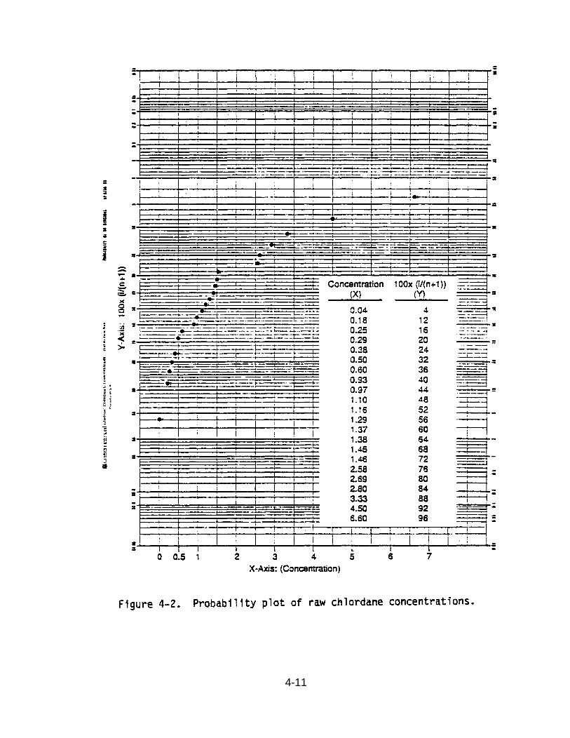
4-11

:~- -,==

Figure 4-2. Probability plot of raw chlordane concentrations.

shape of the curve indicates a lognormal distribution. This is checked in thenext step.

Also, information about the solubility of chlordane in this example ishelpful. Chlordane has a solubility (in water) that ranges between 0.0156 and1.85 mg/L. Because the last six measurements exceed this solubility range,contamination is suspected.

Next, take the natural logarithm of the X-values (1n(X)) (column 5 inTable 4-2). Repeat Step 3 above using the pairs [1in(X), lOOx(i/25)]. The re-sulting plot is shown in Figure 4-3. The points fall approximately on astraight line (hand-drawn) and the hypothesis of lognormality of X, i.e.,1n(X) is normally distributed, can be accepted. The mean can be estimated atslightly below 0 and the standard deviation at about 1.2 on the log scale.

CAUTIONARY NOTE

The probability plot is not a formal test of whether the data follow anormal distribution. It is designed as a quick, graphical procedure toidentify cases of obvious nonnormality. Figure 4-3 is an example of aprobability plot of normal data, illustrating how a probability plot of normaldata looks. Figure 4-2 is an example of how nonnormal data look on a prob-ability plot. Data that are sufficiently nonnormal to require use of a pro-cedure not based on the normal distribution will show a definite curve. Asingle point that does not fall on the straight line does not indicate non-normality, but may be an outlier.

4.2.4 The Chi-Squared Test

The chi-squared test can be used to test whether a set of data properlyfits a specified distribution within a specified probability. Most introduc-tory courses in statistics explain the chi-squared test, and its familiarityamong owners and operators as well as Regional personnel may make it afrequently used method of analysis. In this application the assumed distribu-tion is the normal distribution, but other distributions could also be used.The test consists of defining cells or ranges of values and determining theexpected number of observations that would fall in each cell according to thehypothesized distribution. The actual number of data points in each cell iscompared with that predicted by the distribution to judge the adequacy of thefit.

PURPOSE

The chi-squared test is used to test the adequacy of the assumption ofnormality of the data.

PROCEDURE

Step 1. Determine the appropriate number of cells, K. This numberusually ranges from 5 to 10. Divide the number of observations, N, by 4.Dividing the total number of observations by 4 will guarantee a minimum offour observations necessary for each of the K = N/4 cells. Use the largestwhole number of this result, using 10 if the result exceeds 10.

4-12

_--...-_=__~l ~. -4-A I.._.~±-_.~-.J 1I-+--1-_C=-L.l.j-~+_~- --:--i

;:±:=:i'=t:11i·-r-I/·i';iiii·I~I-~[='==~... __:::::r=:-.:.::::=:

.~ .. "~_~.~-~=.. :'_=" "-.~::-.- · 84%~ ;:;.e: . =-= _ -.~ -~:-- _:..-~.-=!

I -{;:::-; t!,. 1I~---_ >-'.' _~! _ __.__,.+___. --l"

- iI"-~ '- .__.. to-- ;.~

'~t .--. ~- '---r-- ':.:::.-' ,-.' -: 50%.~.• _ ••.::: __a :~4=- ! -=j

1100~ (iI(~+1))i =j.....,--i--+---;--WiW : l:4 ! -~: I 1_

12 I :I

16 =:t:::::::t=:::t:==::t:,=:=:t=t::::t:=:t==L.-20 I !

24323640444852566064687276SOS4S89296

:t-:;==: - .~~~

, r/-

t=--~~:

:~I

In (X)

- E= -3.Zl

~J:::-1.71-1.39-, -1.24

=€ -0.97-0.69_..t:= -0.51

~ -0.07j:=;-~ -0.03~- 0.10L

...J-. 0.15II

~0.25

! 0.31"..,. ":- 0.32:0.37

j == 0.38=~-t= 0.95

.- i--- 0.99.- ,-... -,:= 1.03+ !=== 1.20~ ,,-)C i=:: 1.500 :-= 1.890 E !r--'

II) "I---'x ~- '---< ">- r

'---'-.'=L__' --"!---i-'"'7'-i'-.....,..--+-+---f+---;-'--,..-+-+~-+-_----+--..;.--~_+'--4

I T i/ !

1I1111!AII;I===·~S~:'~L~2i·=_i·l--;lii;'~:I;I;lf=I --+--+ --4~. - --

. -

If0o- l-;'

I

• I

• -3 -2~5 -2 ·1 a 2

X-Axis: In (Concentration)Mean Mean+Std

Figure 4-3. Probability plot of log-transformed chlordane concentrations.

4-13

Step 2. Standardize the data by subtracting the sample mean and divid-ing by the sample standard deviation:

Step 3. Determine the number of observations that fall in each of thecells defined according to Table 4-3. The expected number of observations foreach cell is N/K, where N is the total number of observations and K is thenumber of cells.values from 1 to

Let Ni denote the observed number in cell i (for i takingK)

cell i.and let Ei denote the expected number of observations in

Note that in this case the cells are chosen to make the Ei’s equal.

TABLE 4-3. CELL BOUNDARIES FOR THE CHI-SQUARED TEST

5 6Number of cells (K)

7 8 9 10

Cell boundaries -0.84 -0.97 -1.07 -1.15 -1.22 -1.28for equal ex- -0.25 -0.43 -0.57 -0.67 -1.08 -0.84pected cell 0.25 0.00 -0.18 -0.32 -0.43 -0.52sizes with the 0.84 0.43 0.18 0.00 -0.14 -0.25normal distri- 0.97 0.57 0.32 0.14 0.00bution 1.07 0.67 0.43 0.25

1.15 1.08 0.521.22 0.84

1.28

Step 4. Calculate the chi-squared statistic by the formula below:

Step 5. Compare the calculated result to the table of the chi-squareddistribution with K-3 degrees of freedom (Table 1, Appendix B). Reject thehypothesis of normality if the calculated value exceeds the tabulated value.

REFERENCE

Remington, R. D., and M. A. Schork. Statistics with Applications to theBiological and Health Sciences. Prentice-Hall, 1970. 235-236.

EXAMPLE

The data in Table 4-4 are N = 21 residuals from an analysis of varianceon dioxin concentrations. The analysis of variance assumes that the errors

4-14

TABLE 4-4. EXAMPLE DATA FOR CHI-SQUAREDTEST

Observation ResidualStandardized

residual

-0.45 -1.90-0.35 -1.48-0.35 -1.48-0.22 -0.93-0.16 -0.67-0.13 -0.55-0.11 -0.46-0.10 -0.42-0.10 -0.42-0.06 -0.25-0.05 -0.210.04 0.170.11 0.470.13 0.550.16 0.680.17 0.720.20 0.850.21 0.890.30 1.270.34 1.440.41 1.73

4-15

(estimated by the residuals) are normally distributed. The chi-squared testis used to check this assumption.

Step 1. Divide the number of observations, 21, by 4 to get 5.25. Keeponly the integer part, 5, so the test will use K = 5 cells.

Step 2. The sample mean and standard deviation are calculated and foundto be: X = 0.00, S = 0.24. The data are standardized by subtracting the mean(0 in this case) and dividing by S. The results are also shown in Table 4-4.

Step 3. Determine the number of (standardized) observations that fallinto the five cells determined from Table 4-3. These divisions are: (1) lessthan or equal to -0.84, (2) greater than -0.84 and less than or equal to-0.25, (3) greater than -0.25 and less than or equal to +0.25, (4) greaterthan 0.25 and less than or equal to 0.84, and (5) greater than 0.84. We find4 observations in cell 1, 6 in cell 2, 2 in cell 3, 4 in cell 4, and 5 incell 5.

Step 4. Calculate the chi-squared statistic. The expected number ineach cell is N/K or 21/5 = 4.2.

Step 5. The critical value at the 5% level for a chi-squared test with2 (K-3 = 5-3 = 2) degrees of freedom is 5.99 (Table 1, Appendix 6). Becausethe calculated value of 2.10 is less than 5.99 there is no evidence that thesedata are not normal.

INTERPRETATION

The cell boundaries are determined from the normal distribution so thatequal numbers of observations should fall in each cell. If there are largedifferences between the number of observations in each cell and that predictedby the normal distribution, this is evidence that the data are not normal.The chi-squared statistic is a nonnegative statistic that increases as thedifference between the predicted and observed number of observations in eachcell increases.

If the calculated value of the chi-squared statistic exceeds the tabu-lated value, there is statistically significant evidence that the data do notfollow the normal distribution. In that case, one would need to do a trans-formation, use a nonparametric procedure, or seek consultation before inter-preting the results of the test of the ground-water data. If the calculatedvalue of the chi-squared statistic does not exceed the tabulated criticalvalue, there is no significant lack of fit to the normal distribution and onecan proceed assuming that the assumption of normality is adequately met.

4-16

REMARK

The chi-squared statistic can be used to test whether the residuals froman analysis of variance or other procedure are normal. In this. case thedegrees of freedom are found by (number of cells minus one minus the number ofparameters that have been estimated). This may require more than the sug-gested 10 cells. The chi-squared test does require a fairly large sample sizein that there should be generally at least four observations per cell.

4.3 CHECKING EQUALITY OF VARIANCE: BARTLETT'S TEST

The analysis of variance procedures presented in Section 5 are often moresensitive to unequal variances than to moderate departures from normality.The procedures described in this section allow for testing to determinewhether group variances are equal or differ significantly. Often in practiceunequal variances and nonnormality occur together. Sometimes a transformationto stabilize or equalize the variances also produces a distribution that ismore nearly normal. This sometimes occurs if the initial distribution waspositively skewed with variance increasing with the number of observations.Only Bartlett's test for checking equality, or homogeneity, of variances ispresented here. It encompasses checking equality of more than two varianceswith unequal sample sizes. Other tests are available for special cases. TheF-test is a special situation when there are only two groups to be compared.The user is referred to classical textbooks for this test (e.g., Snedecor andCochran, 1980). In the case of equal sample sizes but more than two variancesto be compared, the user might want to use Hartley's or maximum F-ratio test(see Nelson, 1987). This test provides a quick procedure to test for variancehomogeneity.

PURPOSE

Bartlett's test is a test of homogeneity of variances. In other words,it is a means of testing whether a number of population variances of normaldistributions are equal. Homogeneity of variances is an assumption made inanalysis of variance when comparing concentrations of constituents betweenbackground and compliance wells, or among compliance wells. It should benoted that Bartlett's test is itself sensitive to nonnormality in the data.With long-tailed distributions the test too often rejects equality (homo-geneity) of the variances.

PROCEDURE

Assume that data from k wells are available and that there are ni datapoints for well i.

4-17

thus f is the total sample size minus the number of wells (groups); and

k

Step 3. Using the chi-squared table (Table 1, Appendix B), find thecritical value for X2 with (k-l) degrees of freedom at a predetermined signif-icance level, for example, 5%.

INTERPRETATION

If the calculated value x2 is larger than the tabulated value, then con-clude that the variances are not equal at that significance level.

REFERENCE

Johnson N. L., and F. C. Leone. Statistics and Experimental Design inEngineering and the Physical Sciences. Vol. I, John Wiley and Sons, New York,1977.

EXAMPLE

Manganese concentrations are given for k=6 wells in Table 4-5 below.

Note: Some numbers in Table 4-5 have been rounded.

4-18

TABLE 4-5. EXAMPLE DATA FOR BARTLETT'S TEST

Samplingdate Well 1 Well 2 Well 3 Well 4 Well 5 Well 6

This is the sum of the last line in Table 4-5.

4-19

INTERPRETATION

The sample variances of the data from the six wells were compared bymeans of Bartlett's test. The test was significant at the 5% level, suggest-ing that the variances are significantly unequal (heterogeneous). A log-transform of the data can be done and the same test performed on the trans-formed data. Generally, if the data followed skewed distribution, thisapproach resolves the problem of unequal variances and the user can proceedwith an ANOVA for example.

On the other hand, unequal variances among well data could be a directindication of well contamination, since the individual data could come fromdifferent distributions (i.e., different means and variances). Then the usermay wish to test which variance differs from which one. The reader isreferred here to the literature for a gap test of variance (Tukey, 1949;David, 1956; or Nelson, 1987).

NOTE. In the case of k=2 variances, the test of equality of variances is

the F-test (Snedecor and Cochran, 1980)..

i=l,Bartlett's test simplifies in the case of equal sample sizes, ni=n,

..., k. The test used then is Cochran's test. Cochran's test focuses onthe-largest variance and compares it to the sum of all the variances. Hartleyintroduced a quick test of homogeneity of variances that uses the ratio of thelargest over the smallest variances. Technical aids for the procedures underthe assumption of equal sample sizes are given by L. S. Nelson in the Journalof Quality Technology, Vol. 19, 1987, pp. 107 and 165.

4-20

SECTION 5

BACKGROUND WELL TO COMPLIANCE WELL COMPARISONS

There are many situations in ground-water monitoring that call for thecomparison of data from different wells. The assumption is that a set ofuncontaminated wells can be defined. Generally these are background wells andhave been sited to be hydraulically upgradient from the regulated unit. Asecond set of wells are sited hydraulically downgradient from the regulatedunit and are otherwise known as compliance wells. The data from these com-pliance wells are compared to the data from the background wells to determinewhether there is any evidence of contamination in the compliance wells thatwould presumably result from a release from the regulated unit.

If the owner or operator of a hazardous waste facility does not havereason to suspect that the test assumptions of equal variance or normalitywill be violated, then he or she may simply choose the parametric analysis ofvariance as a default method of statistical analysis. In the event that thismethod indicates a statistically significant difference between the groupsbeing tested, then the test assumptions should be evaluated.

This situation, where the relevant comparison is between data from back-ground wells and data from compliance wells, is the topic of this section.Comparisons between background well data and compliance well data may becalled for in all phases of monitoring. This type of comparison is the gen-eral case for detection monitoring. It is also the usual approach for com-pliance monitoring if the compliance limits are determined by the backgroundwell constituent concentration levels. Compounds that are present in back-ground wells (e.g., naturally occurring metals) are most appropriatelyevaluated using this comparison method.

Section 5.1 provides a flowchart and overview for the selection ofmethods for comparison of background well and compliance well data. Sec-tion 5.2 contains analysis of variance methods. These provide methods fordirectly comparing background well data to compliance well data. Section 5.3describes a tolerance interval approach, where the background well data areused to define the tolerance limits for comparison with the compliance welldata. Section 5.4 contains an approach based on prediction intervals, againusing the background well data to determine the prediction interval for com-parison with the compliance well data. Methods for comparing data to a fixedcompliance limit (an MCL or ACL) will be described in Section 6.

5-l

5.1 SUMMARY FLOWCHART FOR BACKGROUND WELL TO COMPLIANCE WELL COMPARISONS

Figure 5-l is a flowchart to aid in selecting the appropriate statisticalprocedure for background well to compliance well comparisons. The first stepis to determine whether most of the observations are quantified (that is,above the detection limits) or not. Generally, if more than 50% of the obser-vations are below the detection limit (as might be the case with detection orcompliance monitoring for volatile organics) then the appropriate comparisonis a test of proportions. The test of proportions compares the proportion ofdetected values in the background wells to-those in the compliance wells. SeeSection 8.1 for a discussion of dealing with data below the detection limit.

If the proportion of detected values is 50% or more, then an analysis ofvariance procedure is the first choice. Tolerance limits or prediction inter-vals are acceptable alternate choices that the user may select. The analysisof variance procedures give a more thorough picture of the situation at thefacility. However, the tolerance limit or prediction interval approach isacceptable and requires less computation in many situations.

Figure 5-2 is a flowchart to guide the user if a tolerance limitsapproach is selected. The first step in using Figure 5-2 is to determinewhether the facility is in detection monitoring. If so, much of the data maybe below the detection limit. See Section 8.1 for a discussion of this case,which may call for consulting a statistician. If most of the data are quanti-fied, then follow the flow chart to determine if normal tolerance limits canbe used. If the data are not normal (as determined by one of the proceduresin Section 4.2), then the logarithm transformation may be done and the trans-formed data checked for normality. If the log data are normal, the lognormaltolerance limit should be used. If neither the original data nor the log-transformed data are normal, seek consultation with a professionalstatistician.

If a prediction interval is selected as the method of choice, see Sec-tion 5.4 for guidance in performing the procedure.

If analysis of variance is to be used, then continue with Figure 5-l toselect the specific method that is appropriate. A one-way analysis of vari-ance is recommended. If the data show evidence of seasonality (observed, forexample, in a plot of the data over time), a trend analysis or perhaps a two-way analysis of variance may be the appropriate choice. These instances mayrequire consultation with a professional statistician.

If the one-way analysis of variance is appropriate, the computations areperformed, then the residuals are checked to see if they meet the assumptionsof normality and equal variance. If so, the analysis concludes. If not, alogarithm transformation may be tried and the residuals from the analysis ofvariance on the log data are checked for assumptions. If these still do notadequately satisfy the assumptions, then a one-way nonparametric analysis ofvariance may be done, or professional consultation may be sought.

5-2

BACKGROUND WELL TO COMPLIANCE WELL COMPARISONS

(Olhar Possible Approaches),,_L--. • , .__ . ,

Replace NOswllh MOlJ2or PQlJ2

No

No

U1,w

OneWavANOVA

Save Residuals

NonparamelricOne-Way ANOVA

ParamolricOne-WaVANOVA

Figure 5-1. Background well to compl iance well comparisons.

Tolerance Limits: Alternate Approach toBackground Well To Compliance Well Comparisons

Figure 5-2. Tolerance limits: alternate approach to backgroundwell to compliance well comparisons.

5-4

5.2 ANALYSIS OF VARIANCE

If contamination of the ground water occurs from the waste disposalfacility and if the monitoring wells are hydraulically upgradient andhydraulically downgradient from the site, then contamination is unlikely tochange the levels of a constituent in all wells by the same amount. Thus,contamination from a disposal site can be seen as differences in average con-centration among wells, and such differences can be detected by analysis ofvariance.

Analysis of variance (ANOVA) is the name given to a wide variety of sta-tistical procedures. All of these procedures compare the means of differentgroups of observations to determine whether there are any significant differ-ences among the groups, and if so, contrast procedures may be used todetermine where the differences lie. Such procedures are also known in thestatistical literature as general linear model procedures.

Because of its flexibility and power, analysis of variance is the pre-ferred method of statistical analysis when the ground-water monitoring isbased on a comparison of background and compliance well data. The ANOVA isespecially useful in situations where sample sizes are small, as is the caseduring the initial phases of ground-water monitoring. Two types of analysisof variance are presented: parametric and nonparametric one-way analyses ofvariance. Both methods are appropriate when the only factor of concern is thedifferent monitoring wells at a given sampling period.

The hypothesis tests with parametric analysis of variance usually assumethat the errors (residuals) are normally distributed with equal variance.These assumptions can be checked by saving the residuals (the differencebetween the observations and the values predicted by the analysis of variancemodel) and using the tests of assumptions presented in Section 4. Since thedata will generally be concentrations and since concentration data are oftenfound to follow the lognormal distribution, the log transformation is sug-gested if substantial violations of the assumptions are found in the analysisof the original concentration data. If the residuals from the transformeddata do not meet the parametric ANOVA requirements, then nonparametricapproaches to analysis of variance are available using the ranks of the obser-vations. A one-way analysis of variance using the ranks is presented inSection 5.2.2.

When several sampling periods have been used and it is important to con-sider the sampling periods as a second factor, then two-way analysis of vari-ance, parametric or nonparametric, is appropriate. This would be one way totest for and adjust the data for seasonality. Also, trend analysis (e.g.,time series) may be used to identify seasonality in the data set. If neces-sary, data that exhibit seasonal trends can be adjusted. Usually, however,seasonal variation will affect all wells at a facility by nearly the sameamount, and in most circumstances, corrections will not be necessary. Fur-ther, the effects of seasonality will be substantially reduced by simultane-ously comparing aggregate compliance well data to background well data.Situations that require an analysis procedure other than a one-way ANOVAshould be referred to a professional statistician.

5-5

5.2.1 One-Way Parametric Analysis of Variance

In the context of ground-water monitoring, two situations exist for whicha one-way analysis of variance is most applicable:

* Data for a water quality parameter are available from several wellsbut for only one time period (e.g., monitoring has just begun).

* Data for a water quality parameter are available from several wellsfor several time periods. However, the data do not exhibit sea-sonality.

In order to apply a parametric one-way analysis of variance, a minimumnumber of observations is needed to give meaningful results. At least p › 2groups are to be compared (i.e., two or more wells). It is recommended thateach group (here, wells) have at least three observations and that the totalsample size, N, be large enough so that N-p › 5. A variety of combinations ofgroups and number of observations in groups will fulfill this minimum. Onesampling interval with four independent samples per well and at least threewells would fulfill the minimum sample size requirements. The wells should bespaced so as to maximize the probability of intercepting a plume of contamina-tion. The samples should be taken far enough apart in time to guard againstautocorrelation.

PURPOSE

One-way analysis of variance is a statistical procedure to determinewhether differences in mean concentrations among wells, or groups of wells,are statistically significant. For example, is there significant contamina-tion of one or more compliance wells as compared to background wells?

PROCEDURE

Suppose the regulated unit has p wells and that ni data points (concen-trations of a constituent) are available for the ith well. These data can befrom either a single sampling period or from more than one. In the lattercase, the user could check for seasonality before proceeding by plotting thedata over time. Usually the computation will be done on a computer using acommercially available program. However, the procedure is presented so thatcomputations can be done using a desk calculator, if necessary.

(N is the total sample size at this specific regulated unit):

5-6

Observations

Step 2. Compute well totals and well means as follows:

These totals and means

Step 3. Computeand the grand mean:

are shown in the last two columns of the table above.

the sum of squares of differences between well means

(The formula on the far right is usually most convenient for calculation.)This sum of squares has (p-l) degrees of freedom associated with it and is ameasure of the variability between wells.

5-7

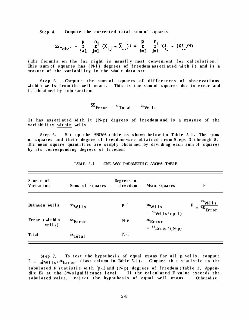
Step 4. Compute the corrected total sum of squares

(The formula on the far right is usually most convenient for calculation.)This sum of squares has (N-l) degrees of freedom associated with it and is ameasure of the variability in the whole data set.

Step 5. -Compute the sum of squares of differences of observationswithin wells from the well means. This is the sum of squares due to error andis obtained by subtraction:

ssError = SSTotal - ssWells

It has associated with it (N-p) degrees of freedom and is a measure of thevariability within wells.

Step 6. Set up the ANOVA table as shown below in Table 5-l. The sumsof squares and their degree of freedom were obtained from Steps 3 through 5.The mean square quantities are simply obtained by dividing each sum of squaresby its corresponding degrees of freedom.

TABLE 5-l. ONE-WAY PARAMETRIC ANOVA TABLE

Source of Degrees ofVariation Sums of squares freedom Mean squares F

Between wells SSWells MSWells FMSWells

= MS= SSWells/(p-l)

Error

Error (within SSError N-Pwells)

MSError= SSError/(N-p)

Total SSTotal N-l

Step 7. To test the hypothesis of equal means for all p wells, computeF = mSWells/MSError (last column in Table 5-l). Compare this statistic to thetabulated F statistic with (p-l) and (N-p) degrees of freedom (Table 2, Appen-dix B) at the 5% significance level. If the calculated F value exceeds thetabulated value, reject the hypothesis of equal well means. Otherwise,

5-8

conclude that there is no significant difference between the concentrations atthe p wells and thus no evidence of well contamination.

In the case of a significant F (calculated F greater than tabulated F inStep 7), the user will conduct the next few steps to determine which compli-ance well(s) is (are) contaminated. This will be done by comparing each com-pliance well with the background well(s). Concentration differences between apair of background wells and compliance wells or between a compliance well anda set of background wells are called contrasts in the ANOVA and multiple com-parisons framework.

Step 8. Determine if the significant F is due to differences betweenbackground and compliance wells (computation of Bonferroni t-statistics).

Assume that of the p wells, u are background wells and m are compliancewells (thus u + m = p). Then m differences--m compliance wells each comparedwith the average of the background wells--need to be computed and tested forstatistical significance. If there are more than five downgradient wells, theindividual comparisons are done at the comparisonwise significance level ofl%, which may make the experimentwise significance level greater than 5%.

•. Obtain the total sample size of all u background wells.

. Compute the average concentration from the u background wells.

. Compute the m differences between the average concentrations fromeach compliance well and the average background wells.

xi . -Xb, i=l,...,m

. Compute the standard error of each difference as

5-9

Compute the m quantities Di = SEi x t for each compliance well i.If m > 5 use the entry for t(N-p),(l-0.0l). That is, use the entryat m = 5.

Step 9. Compute the residuals. The residuals are the differencesbetween each observation and its predicted value according to the particularanalysis of variance model under consideration. In the case of a one-wayanalysis of variance, the predicted value for each observation is the group(that is, well) mean. Thus the residuals are given by:

The residuals, Rij can be used to check for departures from normality asdescribed in Section 4.2.

NOTE

The data can also be checked for equality of variances as described inSection 4.3. The last column of Table 5-2 contains the standard deviationsestimated for each well, the Si used in Bartlett's test.

In some cases it may be appropriate to implement the ANOVA procedureindependently for an individual regulated unit. If there are more than fivewells at the compliance point and the waste management area consists of morethan one regulated unit, then the data may be evaluated separately for eachregulated unit if approved by the Regional Administrator or State Director.In many cases the monitoring well system design and site hydrogeology willdetermine if this approach is appropriate for a particular regulated unit.This will help reduce the number of compliance wells used in a multiple wellcomparisons procedure.

If a single regulated unit has more than five wells at the pointcompliance, refer to the caveat in the cautionary note.

CAUTIONARY NOTE

o f

Should the regulated unit consist of more than five compliance wells,then the Bonferroni t-test should be modified by doing the individual compari-sons at the 1% level so that the Part 264 Subpart F regulatory requirement

5-10

pursuant to §264.97(i)(2) will be met. Alternately, a different analysis ofcontrasts, such as Scheffe's, may be used. The more advanced user is referredto the second reference below for a discussion of multiple comparisons.

REFERENCES

Johnson, Norman L., and F. C. Leone. 1977. Statistics and ExperimentalDesign in Engineering and the Physical Sciences. Vol. II, Second Edition,John Wiley and Sons, New York.

Miller, Ruppert G., Jr. 1981. Simultaneous Statistical Inference. SecondEdition, Springer-Verlag, New York.

EXAMPLE

Four lead concentration values at each of six wells are given inTable 5-2 below. The wells consist of u=2 background and m=4 compliancewells. (The values in Table 5-2 are actually the natural logarithms of theoriginal lead concentrations.)

Step 1. Arrange the 4 x 6 = 24 observations in a data table as follows:

TABLE 5-2. EXAMPLE DATA FOR ONE-WAY PARAMETRIC ANALYSIS OF VARIANCE

Well No.

1 Background wells 4.06 3.99 3.40 3.83 15.28 3.82 0.2962 3.83 4.34 3.47 4.22 15.86 3.97 0.395

Step 2. The calculations are shown on the right-hand side of the datatable above. Sample standard deviations have been computed also.

S t e p 3 . Compute the between-well sum of squares.

with [6 (wells) - l] = 5 degrees of freedom.

5-11

Step 4. Compute the corrected total sum of squares.

with [24 (observations) - 1] = 23 degrees of freedom.

Step 5, Obtain the within-well or error sum of squares by subtraction.

ssError = 11.92 - 5.75 = 6.17

with [24 (observations) - 6 (wells)] = 18 degrees of freedom.

Step 6. Set up the one-way ANOVA as in Table 5-3 below:

TABLE 5-3. EXAMPLE COMPUTATIONS IN ONE-WAY PARAMETRIC ANOVA TABLE

Source of Sums of Degrees ofvariation squares freedom Mean squares F

Between wells 5.76 5 5.76/5 = 1.15 1.15/0.34 = 3.38

Error(within wells)

Total

6.18 18 6.18/18 = 0.34-

11.94 23

Step 7. The calculated F statistic is 3.38. The tabulated F value with5 and 18 degrees of freedom at the a =dix B).

0.05 level is 2.77 (Table 2, Appen-Since the calculated value exceeds the tabulated value, the hypothe-

sis of equal well means must be rejected, and post hoc comparisons arenecessary.

Step 8. Computation of Bonferroni t-statistics.

. Note that there are four compliance wells, so m = 4 comparisons willbe made

5-12

Compute the quantities Dj Again, due to equal sample sizes, theywill al1 be equal.

Di= SEi x t = 0.357 x 2.43 = 0.868 for i = 3,..., 6

Step 9. Compute the residuals using the data given in Table 5-2.

Residuals for Well 1:

= 5.61 - 4.55 = 1.06= 5.14 - 4.55 = 0.59

5-13

R 33 = 3.47 - 4.55 = -1.08R 34 = 3.97 - 4.55 = -0.58

Residuals for Well 4:

= 3.53 - 4.19 = -0.66= 4.54 - 4.19 = 0.35

R 43 = 4.26 - 4.19 = 0.07R4 4

= 4.42 - 4.19 = 0.23

Residuals for Well 5:

R 51 = 3.91 - 4.75 = -0.84R 52 = 4.29 - 4.75 = -0.46R 53 = 5.50 - 4.75 = 0.75R 54 = 5.31 - 4.75 = 0.56

Residuals for Well 6:

R 61 = 5.42 - 5.25 = 0.17R 62 = 5.21 - 5.25 = -0.04R 63 = 5.29 - 5.25 = 0.04R 64 = 5.08 - 5.25 = -0.17

INTERPRETATION

All the compliance well concentrations were somewhat above the mean con-centration of the background levels. The well means should be used to indi-cate the location of the plume. The findings should be reported to theRegional Administrator.

5.2.2 One-Way Nonparametric Analysis of Variance

This procedure is appropriate for interwell comparisons when the data orthe residuals from a parametric ANOVA have been found to be significantly dif-ferent from normal and when a log transformation fails to adequately normalizethe data. In one-way nonparametric ANOVA, the assumption under the nullhypothesis is that the data from each well come from the same continuous dis-tribution and hence have the same median concentrations of a specific hazard-ous constituent. The alternatives of interest are that the data from somewells show increased levels of the hazardous constituent in question.

5-14

The procedure is called the Kruskal-Wallis test. For meaningful results,there should be at least three groups with a minimum sample size of three ineach group. For large data sets use of a computer program is recommended. Inthe case of large data sets a good approximation to the procedure is to re-place each observation by its rank (its numerical place when the data areordered from least to greatest) and perform the (parametric) one-way analysisof variance (Section 5.2.1) on the ranks. Such an approach can be done withsome commercially statistical packages such as SAS.

PURPOSE

The purpose of the procedure is to test the hypothesis that all wells (orgroups of wells) around regulated units have the same median concentration ofa hazardous constituent. If the wells are found to differ, post-hoc compari-sons are again necessary to determine if contamination is present.

Note that the wells define the groups. All wells will have at least fourobservations. Denote the number of groups by K and the number of observationsin each group by nJ, with N being the total number of all observations. LetXiJ denote the jth observation in the ith group, where j runs from 1 to the

number of observations in the group, ni, and i runs from 1 to the number ofgroups, K.

PROCEDURE

Step 1. Rank all N observations of the groups from least to greatest.Let Rij denote the rank of the jth observation in the ith group. As aconvention, denote the background well(s) as group 1.

Step 3. Compute the Kruskal-Wallis statistic:

Step 4. Compare the calculated value H to the tabulated chi-squaredvalue with (K-l) degrees of freedom, where K is the number of groups (Table 1,Appendix B). Reject the null hypothesis if the computed value exceeds thetabulated critical value.

5-15

Step 5. If the computed value exceeds the value from the chi-squaredtable, compute the critical difference for well comparisons to the background,assumed to be group 1:

for i taking values 2,..., K,

where z(a/(K-1)) is the upper (a/(K-l))-percentile from the standard normal

distribution found in.Table 4, Appendix 8. Note: If there are more than fivecompliance wells at the regulated unit (K > 6), use Z.0l, the upper one-percentile from the standard normal distribution.

Step 6. Form the differences of the average ranks for each group to thebackground and compare these with the critical values found in step 5 to de-termine which wells give evidence of contamination. That is, compare Ri-RI toCi for i taking the values 2 through K. (Recall that group 1 is the back-ground.)

While the above steps are the general procedure, some details need to bespecified further to handle special cases. First, it may happen that two ormore observations are numerically equal or tied. When this occurs, determinethe ranks that the tied observations would have received if they had beenslightly different from each other, but still in the same places with respectto the rest of the observations. Add these ranks and divide by the number ofobservations tied at that value to get an average rank. This average rank isused for each of the tied observations. This same procedure is repeated forany other groups of tied observations. Second, if there are any values belowdetection, consider all values below detection as tied at zero. (It isirrelevant what number is assigned to nondetected values as long as all suchvalues are assigned the same number, and it is smaller than any detected orquantified value.)

The effect of tied observations is to increase the value of the sta-tistic, H. Unless there are many observations tied at the same value, theeffect of ties on the computed test statistic is neqligible (in practice, theeffect of ties can probably be neglected unless some group contains 10 percentof the observations all tied, which is most likely to occur for concentrationsbelow detection limit). In the present context, the term "negligible" can bemore specifically defined as follows. Compute the Kruskal-Wallis statisticwithout the adjustment for ties. If the test statistic is significant at the5% level then conclude the test since the statistic with correction for tieswill be significant as well. If the test statistic falls between the 10% andthe 5% critical values, then proceed with the adjustment for ties as shownbelow.

5-16

ADJUSTMENT FOR TIES

If there are 50% or more observations that fell below the detectionlimit, then this method for adjustment for ties is inappropriate. The user isreferred to Section 8 "Miscellaneous Topics." Otherwise, if there are tiedvalues present in the data, use the following correction for the H statistic

H’ = H

l -

REFERENCE

Hollander, Myles, and D. A. Wolfe. 1973. Nonparametric StatisticalMethods. John Wiley and Sons, New York.

EXAMPLE

The data in Table 5-4 represent benzene concentrations in water samplestaken at one background and five compliance wells.

Step 1. The 20 observations have been ranked from least to greatest.The limit of detection was 1.0 ppm. Note that two values in Well 4 were belowdetection and were assigned value zero. These two are tied for the smallestvalue and have consequently been assigned the average of the two ranks 1 and2, or 1.5. The ranks of the observations are indicated in parentheses afterthe observation in Table 5-4. Note that there are 3 observations tied at 1.3that would have had ranks 4, 5, and 6 if they had been slightly different.These three have been assigned the average rank of 5 resulting from averaging4, 5, and 6. Other ties occurred at 1.5 (ranks 7 and 8) and 1.912).

(ranks I1 and

Step 2. The values of the sums of ranks and average ranksat the bottom of Table 5-4.

Step 3. Compute the Kruskal-Wallis statistic

are indicated

5-17

TABL

E 5-

4.EX

AMPL

E DA

TA F

OR O

NE-W

AY N

ONPA

RAME

TRIC

ANO

VA--

BENZ

ENE

CONC

ENTR

ATIO

NS (

ppm

)

Date

Back

grou

ndW

ell 1

Wel

l 2

Com

plia

nce

wel

lsW

ell

3W

ell 4

Well

5We

ll 6

Jan

11.

7 (1

0)11

.0

(20)

1.3

(5)

0 (1

.5)

4.9

(17)

1.6

(9)

Feb

11.

9 (1

1.5)

8.0

(18)

1.2

(3)

1.3

(5)

3.7

(16)

2.5

(15)

Mar

11.

5 (7

.5)

9.5

(19)

1.5

(7.5

)0

(1.5

)2.

3 (1

4)1.

9 (1

1.5)

ADJUSTMENT FOR TIES

There are four groups of ties in the data of Table 5-4:

T1 = (23-2) = 6 for the 2 observations of 1,900.T2 = (23-2) = 6 for the 2 observations of 1,500.

for the 3 observations of 1,300.for the 2 observations of 0.

Step 4. To test the null hypothesis of no contamination, obtain thecritical chi-squared value with (6-l) = 5 degrees of freedom at the 5% signif-icance level from Table 1, Appendix B. The value is 11.07. Compare the cal-culated value, H', with the tabulated value. Since 14.76 is greater than11.07, reject the hypothesis of no contamination at the 5% level. If the sitewas in detection monitoring it should move into compliance monitoring. If thesite was in compliance monitoring it should move into corrective action. Ifthe site was in corrective action it should stay there.

In the case where the hydraulically upgradient wells serve as the back-ground against which the compliance wells are to be compared, comparisons ofeach compliance well with the background wells should be performed in additionto the analysis of variance procedure. In this example, data from each of thecompliance wells would be compared with the background well data. This com-parison is accomplished as follows. The average ranks for each group, Ri. areused to compute differences. If a group of compliance wells for a regulatedunit have larger concentrations than those found in the background wells, theaverage rank for the compliance wells at that unit will be larger than theaverage rank for the background wells.

S t e p 5 . Calculate the critical values to compare each compliance wellto the background well.

In this example, K=6, SQ there are 5 comparisons of the compliance wellswith the background wells. Using an experimentwise significance level of a =0.05, we find the upper 0.05/5 = 0.01 percentile of the standard normaldistribution to be 2.33 (Table 4, Appendix B). The total sample size, N, is20. The approximate critical value, C2, is computed for compliance Well 2,which has the largest average rank, as:

The critical values for the other wells are: 10.5 for Wells 3, 5, and 6; and9.8 for Well 4.

5-19

Step 6. Compute the differences between the average rank of each com-pliance well and the average rank of the background well:

Differences Critical values

Compare each difference with the corresponding critical difference, D2 = 10.5equals the critical value of C2 = 10.5. We conclude that the concentration ofbenzene averaged over compliance Well 2 is significantly greater than that atthe background well. None of the other compliance well concentration ofbenzene is significantly higher than the average background value. Based uponthese results, only compliance Well 2 can be singled out as beingcontaminated.

For data sets with more than 30 observations, the parametric analysis ofvariance performed on the rank values is a good approximation to the Kruskal-Wallis test (Quade, 1966). If the user has access to SAS, the PROC RANK pro-cedure is used to obtain the ranks of the data. The analysis of variance pro-cedure detailed in Section 5.2.1 is then performed on the ranks. Contrastsare tested as in the parametric analysis of variance.

INTERPRETATION

The Kruskal-Wallis test statistic is compared to the tabulated criticalvalue from the chi-squared distribution. If the test statistic does notexceed the tabulated value, there is no statistically significant evidence ofcontamination and the analysis would stop and report this finding. If thetest statistic exceeds the tabulated value, there is significant evidence thatthe hypothesis of no differences in compliance concentrations from the back-ground level is not true. Consequently, if the test statistic exceeds thecritical value, one concludes that there is significant evidence of contami-nation. One then proceeds to investigate where the differences lie, that is,which wells are indicating contamination.

The multiple comparisons procedure described in steps 5 and 6 compareseach compliance well to the background well. This determines which compliancewells show statistically significant evidence of contamination at an experi-mentwise error rate of 5 percent. In many cases, inspection of the mean ormedian concentrations will be sufficient to indicate where the problem lies.

5.3 TOLERANCE INTERVALS BASED ON THE NORMAL DISTRIBUTION

An alternate approach to analysis of variance to determine whether thereis statistically significant evidence of contamination is to use toleranceintervals. A tolerance interval is constructed from the data on (uncontam-inated) background wells. The concentrations from compliance wells are then

5-20

compared with the tolerance interval. With the exception of pH, if the com-pliance concentrations do not fall in the tolerance interval, this providesstatistically significant evidence of contamination.

Tolerance intervals are most appropriate for use at facilities that donot exhibit high degrees of spatial variation between background wells andcompliance wells. Facilities that overlie extensive, homogeneous geologicdeposits (for example, thick, homogeneous lacustrine clays) that do not natu-rally display hydrogeochemical variations may be suitable for this statisticalmethod of analysis.

A tolerance interval establishes a concentration range that is con-structed to contain a specified proportion (P%) of the population with aspecified confidence coefficient, Y. The proportion of the populationincluded, P, is referred to as the coverage. The probability with which thetolerance interval includes the proportion P% of the population is referred toas the tolerance coefficient.

A coverage of 95% is recommended. If this is used, random observationsfrom the same distribution as the background well data would exceed the uppertolerance limit less than 5% of the time. Similarly, a tolerance coefficientof 95% is recommended. This means that one has a confidence level of 95% thatthe upper 95% tolerance limit will contain at least 95% of the distribution ofobservations from background well data. These values were chosen to be con-sistent with the performance standards described in Section 2. The use ofthese values corresponds to the selection of a of 5% in the multiple welltesting situation.

The procedure can be applied with as few as three observations from thebackground distribution. However, doing so would result in a large uppertolerance limit. A sample size of eight or more results is an adequate toler-ance interval. The minimum sampling schedule called for in the regulationswould result in at least four observations from each background well. Only ifa single background well is sampled at a single point in time is the 'samplesize so small as to make use of the procedure questionable.

Tolerance intervals can be constructed assuming that the data or thetransformed data are normally distributed. Tolerance intervals can also beconstructed assuming other distributions. It is also possible to constructnonparametric tolerance intervals using only the assumption that the data camefrom some continuous population. However, the nonparametric toleranceintervals require such a large number of observations to provide a reasonablecoverage and tolerance coefficient that they are impractical in thisapplication.

The range of the concentration data in the background well samples shouldbe considered in determining whether the tolerance interval approach should beused, and if so, what distribution is appropriate. The background well con-centration data should be inspected for outliers and tests of normalityapplied before selecting the tolerance interval approach. Tests of normalitywere presented in Section 4.2. Note that in this case, the test of normalitywould be applied to the background well data that are used to construct the

5-21

tolerance interval. These data should all be from the same normaldistribution.

In this application, unless pH is being monitored, a one-sided toleranceinterval or an upper tolerance limit is desired, since contamination is indi-cated by large concentrations of the hazardous constituents monitored. Thus,for concentrations, the appropriate tolerance interval is (0, TL), with thecomparison of importance being the larger limit, TL.

PURPOSE

The purpose of the tolerance interval approach is to define a concentra-tion range from background well data, within which a large proportion of themonitoring observations should fall with high probability. Once this is done,data from compliance wells can be checked for evidence of contamination by,simply determining whether they fall in the tolerance interval. If they donot, this is evidence of contamination.

In this case the data are assumed to be approximately normally distrib-uted. Section 4.2 provided methods to check for normality. If the data arenot normal, take the natural logarithm of the data and see if the transformeddata are approximately normal. If so, this method can be used on the loga-rithms of the data. Otherwise, seek the assistance of a professionalstatistician.

PROCEDURE

where K is the one-sided normal tolerance factor found in Table 5, Appendix B.

Step 3, Compare each observation from compliance wells to the tolerancelimit found in Step 2. If any observation exceeds the tolerance limit, thatis statistically significant evidence that the well is contaminated. Notethat if the tolerance interval was constructed on the logarithms of the orig-inal background observations, the logarithms of the compliance well observa-tions should be compared to the tolerance limit. Alternatively the tolerancelimit may be transferred to the original data scale by taking the anti-logarithm.

REFERENCE

Lieberman, Gerald J. 1958. "Tables for One-sided Statistical ToleranceLimits." Industrial Quality Control. Vol. XIV, NO. 10.

5-22

EXAMPLE

Table 5-5 contains example data that represent lead concentration levelsin parts per million in water samples at a hypothetical facility. Thebackground well data are in columns 1 and 2, while the other four columnsrepresent compliance well data.

TABLE 5-5. EXAMPLE DATA FOR NORMAL TOLERANCE INTERVAL

Lead concentrations (ppm)

Background well Compliance wellsDate A B Well 1 Well 2 Well 3 Well 4

225.9*183.1*198.3*160.8”

limitis

Step 1. The mean and standard deviation of the n = 8 observations havebeen calculated for the background well. The mean is 51.4 and the standarddeviation is 16.3.

Step 2. The tolerance factor for a one-sided normal tolerance intervalis found from Table 5, Appendix B as 3.188.probability 95% and for n = 8.

This is for 95% coverage withThe upper tolerance limit is then calculated

as 51.4 + (3.188)(16.3) = 103.4.

Step 3. The tolerance limit of 103.3 is compared with the compliancewell data. Any value that exceeds the tolerance limit indicates statisticallysignificant evidence of contamination. Two observations from Well 1, twoobservations from Well 3, and all four observations from Well 4 exceed thetolerance limit. Thus there is statistically significant evidence of con-tamination at Wells 1, 3, and 4.

5-23

INTERPRETATION

A tolerance limit with 95% coverage gives an upper bound below which 95%of the observations of the distribution should fall. The tolerance coeffi-cient used here is 95%, implying that at least 95% of the observations shouldfall below the tolerance limit with probability 95%, if the compliance welldata come from the same distribution as the background data. In other words,in this example, we are 95% certain that 95% of the background lead concentra-tions are below 104 ppm. If observations exceed the tolerance limit, this isevidence that the compliance well data are not from the same distribution, butrather are from a distribution with higher concentrations. This is inter-preted as statistically significant evidence of contamination.

5.4 PREDICTION INTERVALS

A prediction interval is a statistical interval calculated to include oneor more future observations from the same population with a specified confi-dence. This approach is algebraically equivalent to the average replicate(AR) test that is presented in the Technical Enforcement Guidance Document(TEGD), September 1986. In ground-water monitoring, a prediction intervalapproach may be used to make comparisons between background and compliancewell data. This method of analysis is similar to that for calculating atolerance limit, and familiarity with prediction intervals or personal prefer-ence would be the only reason for selecting them over the method for tolerancelimits. The concentrations of a hazardous constituent in the background wellsare used to establish an interval within which K future observations from thesame population are expected to lie with a specified confidence. Then each ofK future observations of compliance well concentrations is compared to theprediction interval. The interval is constructed to contain all of K futureobservations with the stated confidence. If any future observation exceedsthe prediction interval, this is statistically significant evidence of contam-ination. In application, the number of future observations to be collected,K, must be specified. Thus, the prediction interval is constructed for aspecified time period in the future. One year is suggested. The interval canbe constructed either to contain all K individual observations with a speci-fied probability, or to contain the K' means observed at the K' samplingperiods.

The prediction interval presented here is constructed assuming that thebackground data all follow the same normal distribution. If that is not thecase (see Section 4.2 for tests of normality), but a log transformationresults in data that are adequately normal on the log scale, then the intervalmay still be used. In this case, use the data after transforming by takingthe logarithm. The future observations need to also be transformed by takinglogarithms before comparison to the interval. (Alternatively, the end pointsof the interval could be converted back to the original scale by taking theiranti-logarithms.)

PURPOSE

The prediction interval is constructed so that K future compliance wellobservations can be tested by determining whether they lie in the interval or

5-24

not. If not, evidence of contamination is found. Note that the number offuture observations, K, for which the interval is to be used, must be speci-fied in advance. In practice, an owner or operator would need to constructthe prediction interval on a periodic (at least yearly) basis, using the mostrecent background data. The interval is described using the 95% confidencefactor appropriate for individual well comparisons. It is recommended that aone-sided prediction interval be constructed for the mean of the four observa-tions from each compliance well at each sampling period.

PROCEDURE

Step 1. Calculate the mean, x, and the standard deviation, S, for thebackground well data (used to form the prediction interval).

Step 2. Specify the number of future observations for a compliance wellto be included in the interval, K. Then the interval is given by

Step 3. Once the interval has been calculated, at each sampling period,the mean of the m compliance well observations is obtained. This mean is com-pared to see if it falls in the interval. If it does, this is reported andmonitoring continues. If a mean concentration at a sampling period does notfall in the prediction interval, this is statistically significant evidence ofcontamination. This is also reported and the appropriate action taken.

REMARK

For a single future observation, t is given by the t-distribution foundin Table 6 of Appendix B. In general, the interval to contain K future meansof sample size m each is given by

where t is as before from Table 3 of Appendix B and where m is the number ofobservations in each mean. Note that for K single observations, m=l, whilefor the mean of four samples from a compliance well, m=4.

Note, too, that the prediction intervals are one-sided, giving a valuethat should not be exceeded by the future observations. The 5% experimentwisesignificance level is used with the Bonferroni approach. However, to ensure

5-25

that the significance level for the individual comparisons does not go below1 % a/K is restricted to be 1% or larger. If more than K comparisons areused, the comparisonwise significance level of 1% is used, implying that thecomparisonwise level may exceed 5%.

EXAMPLE

Table 5-6 contains chlordane concentrations measured at a hypotheticalfacility. Twenty-four background observations are available and are used todevelop the prediction interval. The prediction interval is applied to K-2sampling periods with m=4 observations at a single compliance well each.

Step 1. Find the mean and standard deviation of the 24 background wellmeasurements. These are 101 and 11, respectively.

Step 2. There are K = 2 future observations of means of 4 observationsto be included in the prediction interval. Entering Table 3 of Appendix B atK = 2 and 20 degrees of freedom (the nearest entry to the 23 degrees offreedom), we find t(20, 2, 0.95) = 2.09. The interval is given by

[0, 101 + (11)2.09(1/4 + 1/24)½ ] = (0, 113.4).

Step 3. The mean of each of the four compliance well observations atsamp ling period one and two is found and compared with the interval found inStep 2. The mean of the first sampling period is 122 and that for the secondsampling period is 113. Comparing the first of these to the prediction inter-val for two means based on samples of size 4, we find that the mean exceedsthe upper limit of the prediction interval. This is statistically significantevidence of contamination and should be reported to the Regional Administra-tor. Since the second sampling period mean is within the prediction interval,the Regional Administrator may allow the facility to remain in its currentstage of monitoring.

INTERPRETATION

A prediction interval is a statistical interval constructed from back-ground sample data to contain a specified number of future observations fromthe same distribution with specified probability. That is, the predictioninterval is constructed so as to have a 95% probability of containing the nextK sampling period means, provided that there is no contamination. If thefuture observations are found to be in the prediction interval, this is evi-dence that there has been no change at the facility and that no contaminationis occurring. If the future observation falls outside of the predictioninterval, this is statistical evidence that the new observation does not comefrom the same distribution, that is, from the population of uncontaminatedwater samples previously sampled. Consequently, if the observation is a con-centration above the prediction interval's upper limit, it is statisticallysignificant evidence of contamination.

5-26

TABLE 5-6. EXAMPLE DATA FOR PREDICTION INTERVAL--CHLORDANE LEVELS

Background well data--Well 1 Compliance well data--Well 2Chlordane Chlordane

Sampling dateconcentration concentration

Sampling date

5-27

The prediction interval could be constructed in several ways. It can bedeveloped for means of observations at each sampling period, or for each in-dividual observation at each sampling period.

It should also be noted that the estimate of the standard deviation, S,that is used should be an unbiased estimator. The usual estimator, presentedabove, assumes that there is only one source of variation. If there are othersources of variation, such as time effects, or spatial variation in the dataused for the background, these should be included in the estimate of the vari-'ability. This can be accomplished by use of an appropriate analysis-of-vari-ance model to include the other factors affecting the variability. Determina-tion of the components of variance in complicated models is beyond the scopeof this document and requires consultation with a professional statistician.

REFERENCE

Hahn, G. and Wayne Nelson. 1973. "A Survey of PredictApplications." Journal of Quality Technology. 5: 178-188.

ion Intervals and Their

5-28

SECTION 6

COMPARISONS WITH MCLs OR ACLs

This section includes statistical procedures appropriate when the moni-toring aims at determining whether ground-water concentrations of hazardousconstituents are below or above fixed concentration limits. In this situationthe maximum concentration limit (MCL) or alternate concentration limit (ACL)is a specified concentration limit rather than being determined by the back-ground well concentrations. Thus the applicable statistical procedures arethose that compare the compliance well concentrations estimated from samplingwith the prespecified fixed limits. Methods for comparing compliance wellconcentrations to a (variable) background concentration were presented inSection 5.

The methods applicable to the type of comparisons described in this sec-tion include confidence intervals and tolerance intervals. A special sectiondeals with cases where the observations exhibit very small or no variability.

6.1 SUMMARY CHART FOR COMPARISON WITH MCLs OR ACLs

Figure 6-1 is a flow chart to aid the user in selecting and applying astatistical method when the permit specifies an MCL or ACL.

As with each type of comparison, a determination is made first to see ifthere are enough data for intra-well comparisons. If so, these should be donein parallel with the other comparisons.

Here, whether the compliance limit is a maximum concentration limit (MCL)or an alternate concentration limit (ACL), the recommended procedure to com-pare the mean compliance well concentration against the compliance limit isthe construction of a confidence interval. This approach is presented inSection 6.2.1. Section 6.2.2 adds a 'special case of limited variance in thedata. If the permit requires that a compliance limit is not to be exceededmore than a specified fraction of the time, then the construction of tolerancelimits is the recommended procedure, discussed in Section 6.2.3.

6.2 STATISTICAL PROCEDURES

This section presents the statistical procedures appropriate for com-parison of ground-water monitoring data to a constant compliance limit, afixed standard. The interpretation of the fixed compliance limit (MCL or ACL)is that the mean concentration should not exceed this fixed limit. An alter-nate interpretation may be specified. The permit could specify a compliancelimit as a concentration not to be exceeded by more than a small, specified

6-1

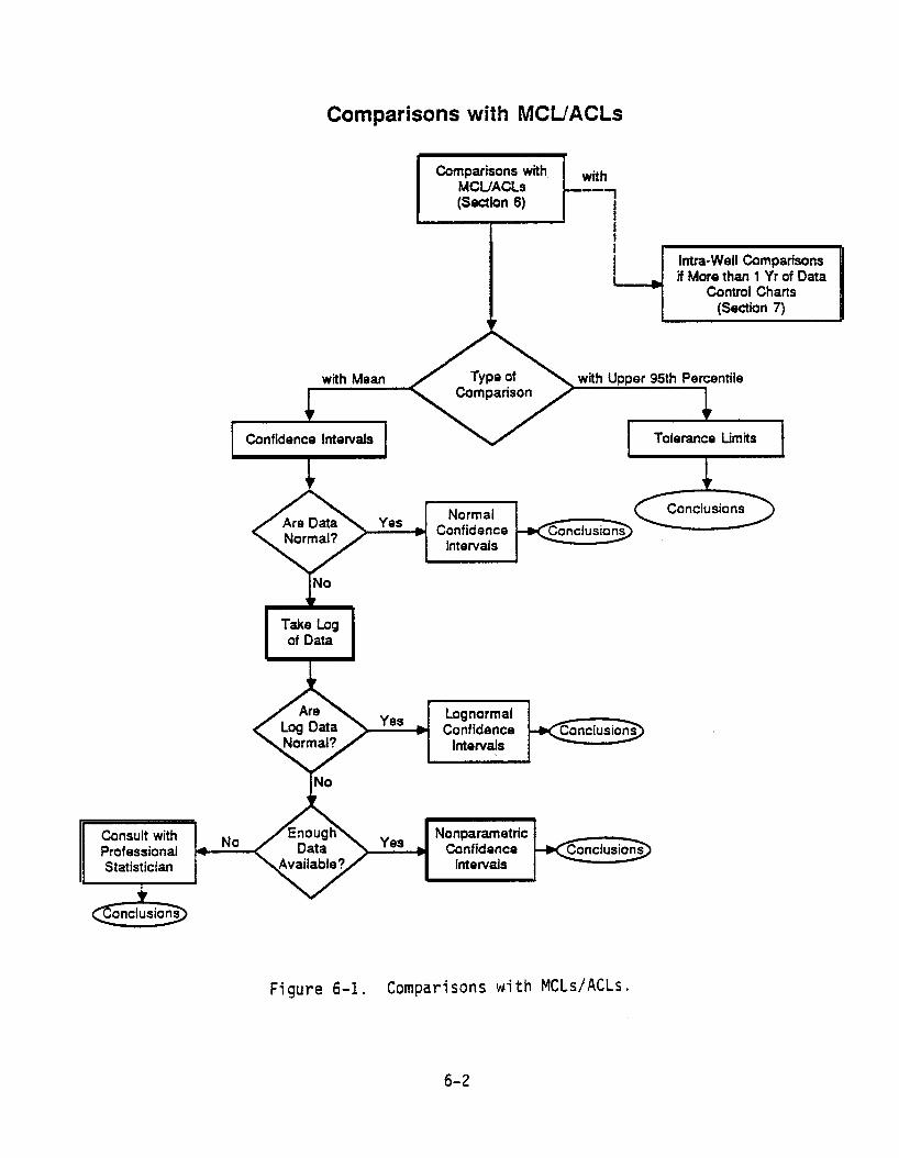
Comparisons with MCUACLs

Comparisons withMCUACLs(Section 6)

with----,

II,I

I Intra-Well Comparisonsif More than 1 Yr of Data

Control Charts(Section 7)

with Mean

Normal>-_Y_es~~ Confidence

Intervals

Take Logof Data

Conclusions

Consult withProfessionalStatistician

No

Yes

Yes

LognormalConfidence

Intervals

NonparametricConfidence

Intervals

Figure 6-1. Comparisons with MCLs/ACLs.

6-2

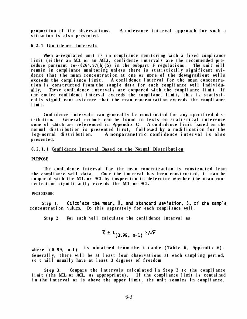
proportion of the observations. A tolerance interval approach for such asituation is also presented.

6.2.1 Confidence Intervals

When a-regulated unit is in compliance monitoring with a fixed compliancelimit (either an MCL or an ACL), confidence intervals are the recommended pro-cedure pursuant to--§264,97(h)(5) in the Subpart F regulations. The unit willremain in compliance monitoring unless there is statistically significant evi-dence that the mean concentration at one or more of the downgradient wellsexceeds the compliance limit. A confidence interval for the mean concentra-tion is constructed from the sample data for each compliance well individu-ally. These confidence intervals are compared with the compliance limit. Ifthe entire confidence interval exceeds the compliance limit, this is statisti-cally significant evidence that the mean concentration exceeds the compliancelimit.

Confidence intervals can generally be constructed for any specified dis-tribution. General methods can be found in texts on statistical inferencesome of which are referenced in Appendix C. A confidence limit based on thenormal distribution is presented first, followed by a modification for thelog-normal distribution. A nonparametric confidence interval is alsopresented.

6.2.1.1 Confidence Interval Based on the Normal Distribution

PURPOSE

The confidence interval for the mean concentration is constructed fromthe compliance well data. Once the interval has been constructed, it can becompared with the MCL or ACL by inspection to determine whether the mean con-centration significantly exceeds the MCL or ACL.

PROCEDURE

Step 1.concentration values. Do this separately for each compliance well.

Step 2. For each well calculate the confidence interval as

where t(0.99, n-l) is obtained from the t-table (Table 6, Appendix 6).Generally, there will be at least four observations at each sampling period,so t will usually have at least 3 degrees of freedom.

Step 3. Compare the intervals calculated in Step 2 to the compliancelimit (the MCL or ACL, as appropriate). If the compliance limit is containedin the interval or is above the upper limit, the unit remains in compliance.

6-3

If any well confidence interval's lower limit exceeds the compliance limit,this is statistically significant evidence of contamination.

REMARK

The 99th percentile of the t-distribution is used in constructing theconfidence interval. This is consistent with an alpha (probability of Type Ierror) of 0.01, since the decision on compliance is made by comparing thelower confidence limit to the MCL or ACL. Although the interval as con-structed with both upper and lower limits is a 98% confidence interval, theuse of it is one-sided, which is consistent with the 1% alpha level ofindividual well comparisons.

EXAMPLE

Table 6-1 lists hypothetical concentrations of Aldicarb in three compli-ance wells. For illustration purposes, the MCL for Aldicarb has been set at7 ppb. There is no evidence of nonnormality, so the confidence interval basedon the normal distribution is used.

TABLE 6-1. EXAMPLE DATA FOR NORMAL CONFIDENCE INTERVAL--ALDICARBCONCENTRATIONS IN COMPLIANCE WELLS (ppb)

Samplingdate Well 1 Well 2 Well 3

MCL = 7 ppb

Step 1. Calculate the mean and standard deviation of the concentrationsfor each compliance well. These statistics are shown in the table above.

Step 2. Obtain the 99th percentile of the t-distribution with (4-l) = 3degrees of freedom from Table 6, Appendix B as 4.541. Then calculate the con-fidence interval for each well's mean concentration.

6-4

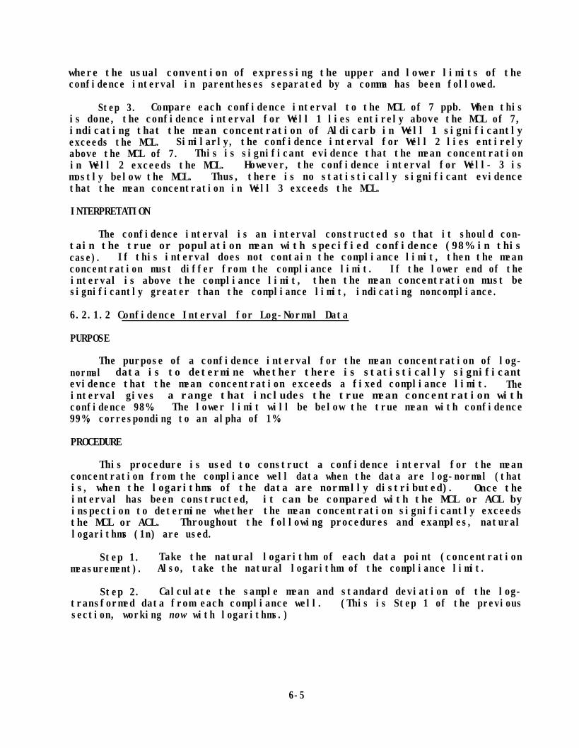
where the usual convention of expressing the upper and lower limits of theconfidence interval in parentheses separated by a comma has been followed.

Step 3. Compare each confidence interval to the MCL of 7 ppb. When thisis done, the confidence interval for Well 1 lies entirely above the MCL of 7,indicating that the mean concentration of Aldicarb in Well 1 significantlyexceeds the MCL. Similarly, the confidence interval for Well 2 lies entirelyabove the MCL of 7. This is significant evidence that the mean concentrationin Well 2 exceeds the MCL. However, the confidence interval for Well- 3 ismostly below the MCL. Thus, there is no statistically significant evidencethat the mean concentration in Well 3 exceeds the MCL.

INTERPRETATION

The confidence interval is an interval constructed so that it should con-tain the true or population mean with specified confidence (98% in thiscase). If this interval does not contain the compliance limit, then the meanconcentration must differ from the compliance limit. If the lower end of theinterval is above the compliance limit, then the mean concentration must besignificantly greater than the compliance limit, indicating noncompliance.

6.2.1.2 Confidence Interval for Log-Normal Data

PURPOSE

The purpose of a confidence interval for the mean concentration of log-normal data is to determine whether there is statistically significantevidence that the mean concentration exceeds a fixed compliance limit. Theinterval gives a range that includes the true mean concentration withconfidence 98%. The lower limit will be below the true mean with confidence99%, corresponding to an alpha of 1%.

PROCEDURE

This procedure is used to construct a confidence interval for the meanconcentration from the compliance well data when the data are log-normal (thatis, when the logarithms of the data are normally distributed). Once theinterval has been constructed, it can be compared with the MCL or ACL byinspection to determine whether the mean concentration significantly exceedsthe MCL or ACL. Throughout the following procedures and examples, naturallogarithms (1n) are used.

Step 1. Take the natural logarithm of each data point (concentrationmeasurement). Also, take the natural logarithm of the compliance limit.

Step 2. Calculate the sample mean and standard deviation of the log-transformed data from each compliance well. (This is Step 1 of the previoussection, working now with logarithms.)

6-5

Step 3. Form the confidence intervals for each compliance well as

where t(o.99,n-1)t will typically

is from the t-distribution in Table 6 of Appendix B. Herehave 3 degrees of freedom.

Step 4. Compare the confidence intervals found in Step 3 to thelogarithm of the compliance limit found in Step 1. If the lower limit of theconfidence interval lies entirely above the logarithm of the compliance limit,there is statistically significant evidence that the unit is out of compli-ance. Otherwise, the unit is in compliance.

EXAMPLE

Table 6-2 contains EDB concentration data from three compliance wells ata hypothetical site. The MCL is assumed to be 20 ppb. For demonstration pur-poses, the data are assumed not normal; a natural log-transformationnormalized them adequately. The lower part of the table contains the naturallogarithms of the concentrations.

TABLE 6-2. EXAMPLE DATA FOR LOG-NORMAL CONFIDENCE INTERVAL--EDBCONCENTRATIONS IN COMPLIANCE WELLS (ppb)

Samplingdate Well 1 Well 2 Well 3

In (MCL) = 3.00

6-6

Step 1. The logarithms of the data are used to calculate a confidenceinterval. Take the natural log of the concentrations in the top part ofTable 6-2 to find the values given in the lower part of the table. For exam-ple, 1n(24.2) = 3.19, . . ., ln(25.3) = 3.23. Also, take the logarithm of theMCL to find that ln(20) = 3.00.

Step 2. Calculate the mean and standard deviation of the log concentra-tions for each compliance well. These are shown in the table.

Step 3. Form the confidence intervals for each compliance well.

where 4.541 is the value obtained from the t-table (Table 6 in Appendix B) asin the previous example.

Step 4. Compare the individual well confidence intervals with the MCL(expressed on the log scale). The natural log of the MCL of 20 ppm is 3.00.None of the individual well confidence intervals for the mean has a lowerlimit that exceeds this value, so none of the individual well mean concentra-tions is significantly different from the MCL.

Note: The lower and upper limits of the confidence interval for eachwell's mean concentration could be converted back to the original scale bytaking antilogs. For example, on the original scale, the confidence intervalswould be:

Well 1: (exp(1.72), exp(4.30)) or (5.58, 73.70)

Well 2: (exp(l.67), exp(5.51)) or (5.31, 262.43)

Well 3: (exp(l.90), exp(5.44)) or (6.69, 230.44)

These limits could be compared directly with the MCL of 20 ppb. It is gen-erally easier to take the logarithm of the MCL rather than the antilogarithmof all of the intervals for comparison.

INTERPRETATION

If the original data are not normal, but the log-transformation ade-quately normalizes the data, the confidence interval (on the log scale) is aninterval constructed so that the lower confidence limit should be less thanthe true or population mean (on the log scale) with specified confidence (99%

6-7

in this case). If the lower end of the confidence interval exceeds the appro-priate compliance limit, then the mean concentration must exceed that compli-ance limit. These results provide statistically significant evidence ofcontamination.

6.2.1.3 Nonparametric Confidence Interval

If the data do not adequately follow the normal distribution even afterthe logarithm transformation, a nonparametric confidence interval can be con-structed. This interval is for the median concentration (which equals themean if the distribution is symmetric). The nonparametric confidence intervalis generally wider and requires more data than the corresponding normal dis-tribution interval, and so the normal or log-normal distribution intervalshould be used whenever it is appropriate. It requires a minimum of seven (7)observations in order to construct an interval with a two-sided confidencecoefficient of 98%, corresponding to a one-sided confidence coefficient of99%. Consequently, it is applicable only for the pooled concentration ofcompliance wells at a single point in time or for special sampling to producea minimum of seven observations at a single well during the sampling period.

PURPOSE

The nonparametric confidence interval is used when the raw data have beenfound to violate the normality assumption, a log-transformation fails tonormalize the data, and no other specific distribution is assumed. It pro-duces a simple confidence interval that is designed to contain the true orpopulation median concentration with specified confidence (here 99%). If thisconfidence interval contains the compliance limit, it is concluded that themedian concentration does not differ significantly from the compliancelimit. If the interval's lower limit exceeds the compliance limit, this isstatistically significant evidence that the concentration exceeds the compli-ance limit and the unit is out of compliance.

PROCEDURE

Step 1. Within each compliance well, order the n data from least togreatest, denoting the ordered data by X(l),..., X(n), where X(i) is the ithvalue in the ordered data.

Step 2. Determine the critical values of the order statistics asfollows. If the minimum seven observations is used, the critical values are 1and 7. Otherwise, find the smallest integer, M, such that the cumulativebinomial distribution with Parameters n (the sample size) and D = 0.5 is atleas

take

t 0.99. Table 6-3 gives' the values of M and n+l-M together with the exact confidence coefficient for sample sizes from 4 to 11. For larger samples,as an approximation the nearest integer value to

M

where Z0.99 is the 99th percentile from the normal distribution (Table 4,Appendix B) and equals 2.33.

6-8

TABLE 6-3. VALUES OF M AND n+I-M AND CONFIDENCECOEFFICIENTS FOR SMALL SAMPLES

M n+l-MTwo-sidedconfidence

87.5%93.8%96.9%98.4%99.2%99.6%97.9%98.8%

Step 3. Once M has been determined in Step 2, find n+l-M and take as theconfidence limits the order statistics, X(M) and X(n+l-M). (With the minimumseven observations, use X(1) and X(7).)

Step 4. Compare the confidence limits found in Step 3 to the compliancelimit. If the lower limit, X(M) exceeds the compliance limit, there is sta-tistically significant evidence of contamination. Otherwise, the unit remainsin compliance.

REMARK

The nonparametric confidence interval procedure requires at least sevenobservations in order to obtain a (one-sided) significance level of 1% (confi-dence of 99%). This means that data from two (or more) wells or samplingperiods would have to be pooled to achieve this level. If only the fourobservations from one well taken at a single sampling period were used, theone-sided significance level would be 6.25%. This would also be the falsealarm rate.

Ties do not affect the procedure. If there are ties, order the observa-tions as before, including all of the tied values as separate observations.That is, each of the observations with a common value is included in theordered list (e.g., 1, 2, 2, 2, 3, 4, etc.). For ties, use the average of thetied ranks as in Section 5.2.2, Step 1 of the example. The ordered statisticsare found by counting positions up from the bottom of the list as before.Multiple values from separate observations are counted separately.

EXAMPLE

Table 6-4 contains concentrations of T-29 in parts per million from twohypothetical compliance wells. The data are assumed to consist of four sam-ples taken each quarter for a year, so that sixteen observations are available

6-9

TABLE 6-4. EXAMPLE DATA FOR NONPARAMETRIC CONFIDENCEINTERVAL--T-29 CONCENTRATIONS (ppm)

Well 1 Well 2Sampling Concentration Concentration

date (ppm) Rank (ppm) Rank

from each well. The data are not normally distributed, neither as raw datanor when log transformed. Thus, the nonparametric confidence interval isused. The MCL is taken to be 15 ppm.

Step 1. Order the 16 measurements from least to greatest within eachwell separately. The numbers in parentheses beside each concentration inTable 6-4 are the ranks or order of the observation. For example, in Well 1,the smallest observation is 2.32, which has rank 1. The second smallest is3.17, which has rank 2, and so forth, with the largest observation of 21.36having rank 16.

Step 2. The sample size is large enough so that the approximation isused to find M.

Step 3. The approximate 95% confidence limits are given by the16 + 1 - 14 = 3rd largest observation and the 14th largest observation. For

6-10

Well 1, the 3rd observation is 3.39 and the 14th largest observation is10.25. Thus the confidence limits for Well 1 are (3.39, 10.25). Similarlyfor Well 2, the 3rd largest observation and the 14th largest observation arefound to give the confidence interval (2.20, 11.02). Note that for Well 2there were two values below detection. These were assigned a value of zeroand received the two smallest ranks. Had there been three or more valuesbelow the limit of detection, the lower limit of the confidence interval wouldhave been the limit of detection because these values would have been thesmallest values and so would have included the third order statistic.

Step 4. Neither of the two confidence intervals' lower limit exceeds theMCL of 15. In fact, the upper limit is less than the MCL, implying that theconcentration in each well is significantly below the MCL.

INTERPRETATION

The rank-order statistics used to form the confidence interval in thenonparametric confidence interval procedure will contain the population medianwith confidence coefficient of 98%. The population median equals the meanwhenever the distribution is symmetric. The nonparametric confidence intervalis generally wider and requires more data than the corresponding normal dis-tribution interval, and so the normal or log-normal distribution intervalshould be used whenever it is appropriate.

If the confidence interval contains the compliance limit (either MCL orACL), then it is reasonable to conclude that the median compliance well con-centration does not differ significantly from the compliance limit. If thelower end of the confidence interval exceeds the compliance limit, this isstatistically significant evidence at the 1% level that the median compliancewell concentration 'exceeds the compliance limit and the unit is out ofcompliance.

6.2.2 Tolerance Intervals for Compliance Limits

In some cases a permit may specify that a compliance limit (MCL or ACL)is not to be exceeded more than a specified fraction of the time. Since lim-ited data will be available from each monitoring well, these data can be usedto estimate a tolerance interval for concentrations from that well. If theupper end of the tolerance interval (i.e., upper tolerance limit) is less thanthe compliance limit, the data indicate that the unit is in compliance. Thatis, concentrations should be less than the compliance limit at least a speci-fied fraction of the time. If the upper tolerance limit of the intervalexceeds the compliance limit, then the concentration of the hazardous con-stituent could exceed the compliance limit more than the specified proportionof the time.

This procedure compares an upper tolerance limit to the MCL or ACL. Withsmall sample sizes the upper tolerance limit can be fairly large, particularlyif large coverage with high confidence is desired. If the owner or operatorwishes to use a tolerance limit in this application, he/she should suggestvalues for the parameters of the procedure subject to the approval of theRegional Administrator. For example, the owner or operator could suggest a

6-11

95% coverage with 95% confidence. This means that the upper tolerance limitis a value which, with 95% confidence, will be exceeded less than 5% of thetime.

PURPOSE

The purpose of the tolerance interval approach is to construct an inter-val that should contain a specified fraction of the concentration measurementsfrom compliance wells with a specified degree of confidence. In this appli-cation it is generally desired to have the tolerance interval contain 95% ofthe measurements of concentration with confidence at least 95%.

PROCEDURE

It is assumed that the data used to construct the tolerance interval areapproximately normal. The data may consist of the concentration measurementsthemselves if they are adequately normal (see Section 4.2 for tests of normal-ity), or the data used may be the natural logarithms of the concentrationdata. It is important that the compliance limit (MCL or ACL) be expressed inthe same units (either concentrations or logarithm of the concentrations) asthe observations.

Step 1.compliance well concentration data.

Table 5, Appendix B contains the factors for a 95% coverage tolerance intervalwith confidence factor 95%.

Step 3. Compare the upper limit of the tolerance interval computed inStep 2 to the compliance limit. If the upper limit of the tolerance intervalexceeds that limit, this is statistically significant evidence of contamina-tion.

EXAMPLE

Table 6-5 contains Aldicarb concentrations at a hypothetical facility incompliance monitoring. The data are concentrations in parts per million (ppm)and represent observations at three compliance wells. Assume than the permitestablishes an ACL of 50 ppm that is not to be exceeded more than 5% of thetime.

Step 1. Calculate the mean and standard deviation of the observationsfrom each well. These are given in the table.

6-12

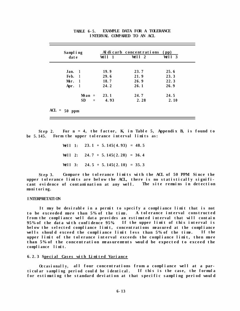
TABLE 6-5. EXAMPLE DATA FOR A TOLERANCEINTERVAL COMPARED TO AN ACL

Samplingdate

Aldicarb concentrations (pp)Well 1 Well 2 Well 3

Jan. 1 19.9 23.7 25.6Feb. 1 29.6 21.9 23.3Mar. 1 18.7 26.9 22.3Apr. 1 24.2 26.1 26.9

Mean = 23.1 24.7 24.5SD = 4.93 2.28 2.10

ACL = 50 ppm

Step 2. For n = 4, the factor, K, in Table 5, Appendix B, is found tobe 5.145. Form the upper tolerance interval limits as:

Well 1: 23.1 + 5.145(4.93) = 48.5

Well 2: 24.7 + 5.145(2.28) = 36.4

Well 3: 24.5 + 5.145(2.10) = 35.3

Step 3. Compare the tolerance limits with the ACL of 50 PPM. Since theupper tolerance limits are below the ACL, there is no statistically signifi-cant evidence of contamination at any well. The site remains in detectionmonitoring.

INTERPRETATION

It may be desirable in a permit to specify a compliance limit that is notto be exceeded more than 5% of the time. A tolerance interval constructedfrom the compliance well data provides an estimated interval that will contain95% of the data with confidence 95%. If the upper limit of this interval isbelow the selected compliance limit, concentrations measured at the compliancewells should exceed the compliance limit less than 5% of the time. If theupper limit of the tolerance interval exceeds the compliance limit, then morethan 5% of the concentration measurements would be expected to exceed thecompliance limit.

6.2.3 Special Cases with Limited Variance

Occasionally, all four concentrations from a compliance well at a par-ticular sampling period could be identical. If this is the case, the formulafor estimating the standard deviation at that specific sampling period would

6-13

give zero, and the methods for calculating parametric confidence intervalswould give the same limits for the upper and lower ends of the intervals,which is not appropriate.

In the case of identical concentrations, one should assume that there issome variation in the data, but that the concentrations were rounded and givethe same values after rounding- To account for the variability that waspresent before rounding, take the least significant digit in the reportedconcentration as having resulted from rounding. Assume that rounding resultsin a uniform error on the interval centered at the reported value with theinterval ranging up or down one half unit from the reported value. Thisassumed rounding is used to obtain a nonzero estimate of the variance for usein cases where all the measured concentrations were found to be identical.

PURPOSE

The purpose of this procedure is to obtain a nonzero estimate of thevariance when all observations from a well during a given sampling period gaveidentical results. Once this modified variance is obtained, its square rootis used in place of the usual sample standard deviation, S, to construct con-fidence intervals or tolerance intervals.

PROCEDURE

Step 1. Determine the least significant value of any data point. Thatis, determine whether the data were reported to the nearest 10 ppm, nearest 1ppm, nearest 100 ppm, etc. Denote this value by 2R.

Step 2. The data are assumed to have been rounded to the nearest 2R, soeach observation is actually the reported value ±R. Assuming that the obser-vations were identical because of rounding, the variance is estimated to beR2/3, assuming the uniform distribution for the rounding error. This givesthe estimated standard deviation as

Step 3. Take this estimated value from Step 2 and use it as the estimateof the standard deviation in the appropriate parametric procedure. That is,replace S by S'.

EXAMPLE

In calculating a confidence interval for a single compliance well, sup-pose that four observations were taken during a sampling period and allresulted in 590 ppm. There is no variance among the four values 590, 590,590, and 590.

Step 1. Assume that each of the values 590 came from rounding the con-centration to the nearest 10 ppm. That is, 590 could actually be any valuebetween 585.0 and 594.99. Thus, 2R is 10 ppm (rounded off), so R is 5 ppm.

6-14

Step 2. The estimate of the standard deviation is

as the 98% confidence interval of the average concentration. Note that 4.541is the 99th percentile from the t-distribution (Table 6, Appendix B) with 3degrees of freedom since the sample size was 4.

INTERPRETATION

When identical results are obtained from several different samples, theinterpretation is that the data are not reported to enough significant figuresto show the random differences. If there is no extrinsic evidence invalidat-ing the data, the data are regarded as having resulted from rounding moreprecise results to the reported observations, The rounding is assumed toresult in variability that follows the uniform distribution on the range ±R,where 2R is the smallest unit of reporting. This assumption is used to calcu-late a standard deviation for the observations that otherwise appear to haveno variability.

REMARK

Assuming that the data are reported correctly to the units indicated,other distributions for the rounding variability could be assumed. The max-imum standard deviation that could result from rounding when the observationis ±R is the value R.

6-15

SECTION 7

CONTROL CHARTS FOR INTRA-WELL COMPARISONS

The previous sections cover various situations where the compliance welldata are compared to the background well data or to specified concentrationlimits (ACL or MCL) to detect possible contamination. This section discussesthe case where the level of each constituent within a single uncontaminatedwell is being monitored over time. In essence, the data for each constituentin each well are plotted on a time scale and inspected for obvious featuressuch as trends or sudden changes in concentration levels. The method sug-gested here is a combined Shewhart-CUSUM control chart for each well andconstituent.

The control chart method is recommended for uncontaminated wells only,when data comprising at least eight independent samples over a one-year periodare available. This requirement is specified under current RCRA regulationsand applies to each constituent in each well.

As discussed in Section 2, a common sampling plan will obtain four inde-pendent samples from each well on a semi-annual basis. With this plan a con-trol chart can be implemented when one year's data are available. As a resultof Monte Carlo simulations, Starks (1988) recommended at least four samplingperiods at a unit of eight or more wells, and at least eight sampling periodsat a unit with fewer than four wells.

The use of control charts can be an effective technique for monitoringthe levels of a constituent at a given well over time. It also provides avisual means of detecting deviations from a "state of control." It is clearthat plotting of the data is an important part of the analysis process. Plot-ting is an easy task, although time-consuming if many data sets need to beplotted. Advantage should be taken of graphics software, since plotting oftime series data will be an ongoing process. New data points will be added tothe already existing data base each time new data are available. The follow-ing few sections will discuss, in general terms, the advantages of plottingtime series data; the corrective steps one could take to adjust when season-ality in the data is present; and finally, the detailed procedure for con-structing a Shewhart-CUSUM control chart, along with a demonstration of thatprocedure, is presented.

7.1 ADVANTAGES OF PLOTTING DATA

While analyzing the data by means of any of the appropriate statistica?procedures discussed in earlier sections is recommended, we also recommendplotting the data. Each data point should be plotted against time using atime scale (e.g., month, quarter). A plot should be generated for each

7-l

constituent measured in each well. For visual comparison purposes, the scaleshould be kept identical from well to well for a given constituent.

Another important application of the plotting procedure is for detectingpossible trends or drifts in the data from a given well. Furthermore, whenvisually comparing the plots from several wells within a unit, possible con-tamination of one rather than all downgradient wells could be detected whichwould then warrant a closer look at that well. In general, graphs can providehighly effective illustrations of the time series, allowing the analyst toobtain a much greater sense of the data. Seasonal fluctuations or suddenchanges, for example, may become quite evident, thereby supporting the analystin his/her decision of which statistical procedure to use. General upward ordownward trends, if present, can be detected and the analyst can follow-upwith a test for trend, such as the nonparametric Mann-Kendall test (Mann,1945; Kendall, 1975). If, in addition, seasonality is suspected, the user canperform the seasonal Kendall test for trend developed by Hirsch et al.(1982). The reader is also referred to Chapters 16 "Detecting and EstimatingTrends" and 17 "Trends and Seasonality" of Gilbert's "Statistical Methods forEnvironmental Pollution Monitoring," 1987. In any of the above cases, thehelp of a professional statistician is recommended.

Another important use of data plots is that of identifying unusual datapoints (e.g., outliers). These points should then be investigated for pos-sible QC problems, data entry errors, or whether they are truly outliers.

Many software packages are available for computer graphics, developed formainframes, mini-, or microcomputers. For example, SAS features an easy-to-use plotting procedure, PROC PLOT; where the hardware and software are avail-able, a series of more sophisticated plotting routines can be accessed throughSAS GRAPH. On microcomputers, almost everybody has his or her favoritegraphics software that they use on a regular basis and no recommendation willbe made as to the most appropriate one. The plots shown in this document weregenerated using LOTUS l-2-3.

Once the data for each constituent and each well are plotted, the plotsshould be examined for seasonality and a correction is recommended shouldseasonality be present. A fairly simple-to-use procedure for deseasonalizingdata is presented in the following paragraphs.

7.2 CORRECTING FOR SEASONALITY

A necessary precaution before constructing a control chart is to takeinto account seasonal variation of the data to minimize the chance of mistak-ing seasonal effect for evidence of well contamination. This could resultfrom variations in chemical concentrations with recharge rates duringdifferent seasons throughout the years. If seasonality is present, thendeseasonalizing the data prior to using the combined Shewhart-CUSUM controlchart procedure is recommended.

Many approaches to deseasonalize data exist. If the seasonal pattern isregular, it may be modeled with a sine or cosine function. Moving averagescan be used, or differences (of order 12 for monthly data for example) can be

7-2

used. However, time series models may include rather complicated methods fordeseasonalizing the data. Another simpler method exists which should be ade-quate for the situations described in this document. It has the advantage ofbeing easy to understand and apply, and of providing natural estimates of themonthly or quarterly effects via the monthly or quarterly means. The methodproposed here can be applied to any seasonal cycle--typically an annual cyclefor monthly or quarterly data.

NOTE

Corrections for seasonality should be used with great caution as theyrepresent extrapolation into the future. There should be a good scientificexplanation for the seasonality as well as good empirical evidence for theseasonality before corrections are made. Larger than average rainfalls fortwo or three Augusts in a row does not justify the belief that there willnever be a drought in August, and this idea extends directly to groundwaterqua1ity. In addition, the quality (bias, robustness, and-variance) of theestimates of the proper corrections must be considered even in cases wherecorrections are called for. If seasonality is suspected, the user might wantto seek the help of a professional statistician.

PURPOSE

When seasonality is known to exist in a time series of concentrations,then the data should be deseasonalized prior to constructing control charts inorder to take into account seasonal variation rather than mistaking seasonaleffects for evidence of contamination.

PROCEDURE

The following instructions to adjust a time series for seasonality arebased on monthly data with a yearly cycle. The procedure can be easily modi-fied to accommodate a yearly cycle of quarterly data.

Assume that N years of monthly data are available. Let Xij denote theunadjusted observation for the ith month during the jth year.

Step 1. Compute the average concentration for month i over the N-yearperiod:

This is the average of all observations taken in different years but duringthe same month. That is, calculate the mean concentrations for all Januarys,then the mean for all Februarys and so on for each of the 12 months.

Step 2. Calculate the grand mean,

7-3

January 1.99 2.01 2.15 2.05 2.10 2.13 2.27February 2.10 2.10 2.17 2.12 2.14 2.15 2.21March 2.12 2.17 2.27 2.19 2.10 2.15 2.25April 2.12 2.13 2.23 2.16 2.13 2.14 2.24May 2.11 2.13 2.24 2.16 2.12 2.13 2.25June 2.15 2.18 2.26 2.20 2.12 2.15 2.23July 2.19 2.25 2.31 2.25 2.11 2.16 2.23August 2.18 2.24 2.32 2.25 2.10 2.16 2.24September 2.16 2.22 2.28 2.22 2.11 2.17 2.22October 2.08 2.13 2.22 2.14 2.10 2.16 2.24November 2.05 2.08 2.19 2.11 2.11 2.14 2.25December 2.08 2.16 2.22 2.16 2.09 2.17 2.23

Overall 3-year average = 2.17

Step 3. Compute the adjusted concentrations,

EXAMPLE

Columns 2 through 4 of Table 7-l show monthly unadjusted concentrationsof a fictitious analyte over a 3-year period.

TABLE 7-l. EXAMPLE COMPUTATION FOR DESEASONALIZING DATA

Unadjustedconcentrations

1983 1984 19853-Monthaverage

Monthly adjustedconcentrations

1983 1984 1985

Step 1. Compute the monthly averages across the 3 years. These valuesare shown in the fifth column of Table 7-l.

Step 2. The grand mean over the 3-year period is calculated to be 2.17

7-4

Step 3. Within each month and year, subtract the average monthly con-centration for that month and add the grand mean. For example, for January1983, the adjusted concentration becomes

1.99 - 2.05 + 2.17 = 2.11

The adjusted concentrations are shown in the last three columns

The reader can check that the average of all 36 adjusted

of Table 7-l.

concentrationsshows the plotequals 2.17, the average unadjusted concentration. Figure 7-1

of the unadjusted and adjusted data. The raw data clearly exhibit seasonalityas well as an upwards trend which is less evident by simply looking at thedata table.

INTERPRETATION

As can be seen in Figure 7-1, seasonal effects were present in thedata. After adjusting for monthly effects, the seasonality was removed as canbe seen in the adjusted data plotted in the same figure.

7.3 COMBINED SHEWHART-CUSUM CONTROL CHARTS FOR EACH WELL AND CONSTITUENT

Control charts are widely used as a statistical tool in industry as wellas research and development laboratories. The concept of control charts isrelatively simple, which makes them attractive to use. From the populationdistribution of a given variable, such as concentrations of a given constit-uent, repeated random samples are taken at intervals over time. Statistics,for example the mean of replicate values at a point in time, are computed andplotted together with upper and/or lower predetermined limits on a chart wherethe x-axis represents time. If a result falls outside these boundaries, thenthe process is declared to be "out of control"; otherwise, the process isdeclared to be "in control." The widespread use of control charts is due totheir ease of construction and the fact that they can provide a quick visualevaluation of a situation, and remedial action can be taken, if necessary.

In the context of ground water monitoring, control charts can be used tomonitor the inherent statistical variation of the data collected within asingle well, and to flag anomalous results. Further investigation of datapoints lying outside the established boundaries will be necessary before anydirect action is taken.

A control chart that can be used on a real time basis must be constructedfrom a data set large enough to characterize the behavior of a specificwell. It is recommended that data from a minimum of eight samples within ayear be collected for each constituent at each well to permit an evaluation ofthe consistency of monitoring results with the current concept of the hydro-geology of the site. Starks (1988) recommends a minimum of four samplingperiods at a unit with eight or more wells and a minimum of eight samplingperiods at a unit with less than four wells. Once the control chart for thespecific constituent at a given well is acceptable, then subsequent data

7-5

2.3

2

2.3

2.2

8

2.2

6

2.2

4

2.2

2

2.2

2.1

8

2.1

6

2.1

4

2.1

2

2.1

2.0

8

2.0

6

2.0

4

2.0

2 2

1.98

Tim

e S

eri

es

of

Mo

nth

ly O

bse

rva

tio

ns

(Un

adju

sted

, A

dju

sted

, 3-

year

Mea

n)

--

Ja

n-8

3

Ma

y-8

3

Se

p-8

3

Ja

n-8

4

Ma

y-8

4

Se

p-8

4

Ja

n-8

5M

ay

-85

S

ep

-85

Tim

e (m

on

th)

aU

nadj

uste

d+

Adj

uste

d--

----

3-y

ea

r M

ea

n

Figu

re 7

-1.

Plot

of

unad

just

ed a

nd s

easo

nall

y ad

just

ed m

onth

ly o

bser

vati

ons.

points can be plotted onprocess is in control.

it to provide a quick evaluation as to whether the

The standard assumptionsgenerated by the process,

in the use of control charts are that the datawhen it is in control, are independently (see Sec-

tion 2.4.2) and normally distributed with a fixed mean µ and constant varianceó2. The most important assumption is that of independence; control charts arenot robust with respect to departure from independence (e.g., serial correla-tion, see glossary). In general, the sampling scheme will be such that thepossibility of obtaining serially correlated results is minimized, as noted inSection 2. The assumption of normality is of somewhat less concern, butshould be investigated before plotting the charts. A transformation (e.g.,log-transform, square root transform) can be applied to the raw data so as toobtain errors normally distributed about the mean. An additional situationwhich may decrease the effectiveness of control charts is seasonality in thedata. The problem of seasonality can be handled by removing the seasonalityeffect from the data, provided that sufficient data to cover at least twoseasons of the same type are available (e.g., 2 years when monthly or quart-erly seasonal effect). A procedure to correct a time series for seasonalitywas shown above in Section 7.2.

PURPOSE

Combined Shewhart-cumulative sum (CUSUM) control charts are constructedfor each constituent at each well to provide a visual tool of detecting bothtrends and abrupt changes in concentration levels.

PROCEDURE

Assume that data from at least eight independent samples of monitoringare available to provide reliable estimates of the mean, µ, and standarddeviation, ó, of the constituent's concentration levels in a given well.

Step 1. To construct a combined Shewhart-CUSUM chart, three parametersneed to be selected prior to plotting:

h - a decision internal value

SCLa reference value- Shewhart control limit (denoted by U in Starks (1988))

The parameter k of the CUSUM scheme is directly obtained from the value,D, of the displacement that should be quickly detected; k = D/2. It is recom-mended to select k = 1, which will allow a displacement of two standard devia-tions to be detected quickly.

When k is selected to be 1, the parameter h is usually set at values of 4or 5. The parameter h is the value against which the cumulative sum in theCUSUM scheme will be compared. In the context of groundwater monitoring, avalue of h = 5 is recommended (Starks, 1988; Lucas, 1982).

7-7

The upper Shewhart limit is set at SCL = 4.5 in units of standard devia-tion. This combination of k = 1, h = 5, and SCL = 4.5 was found most appro-priate for the application of combined Shewhart-CUSUM charts for groundwatermonitoring (Starks, 1988).

Step 2.X X

Assume that at time period Ti, ni concentration measurements1, . ..) ni, are available. Compute their average Xi.

Step 3. Calculate the standardized mean

where µ and ó are the mean and standard deviation obtained from prior monitor-ing at the same well (at least four sampling periods in a year).

Step 4. At each time period, Ti, compute the cumulative sum, Si, as:

Si = max [O, (Zi - k) + Si-1)

where max {A, B) is the maximum of A and B, starting with S0 = 0.

Step 5. Plot the values of Si versus Ti on a time chart for this com-bined Shewhart-CUSUM scheme. Declare an "out-of-control" situation at sam-pling period Ti if for the first time, Si > h or Zi › SCL. This will indicateprobable contamination at the well and further investigations will benecessary.

REFERENCES

Lucas, J. M. 1982. "Combined Shewhart-CUSUM Quality Control Schemes." JOur-nal of Quality Technology. Vol. 14, pp. 51-59.

Starks, T. H. 1988 (Draft). "Evaluation of Control Chart Methodologies forRCRA Waste Sites."

Hockman, K. K., and J. M. Lucas. 1987. "Variability Reduction Through Sub-vessel CUSUM Control.' Journal of Quality Technology. Vol. 19, pp. 113-121.

EXAMPLE

The procedure is demonstrated on a set of carbon tetrachloride measure-ments taken monthly at a compliance well over a l-year period. The monthlymeans of two measurements each (n = 2 for all i's) are presented in the thirdcolumn of Table 7-2 below. Estimates of µ or and ó, the mean and standarddeviation of carbon tetrachloride measurements at that particular well wereobtained from a preceding monitoring period at that well; µ = 5.5 µg/L anda = 0.4 µg/L.

7-8

TABLE 7-2. EXAMPLE DATA FOR COMBINED SHEWHART-CUSUM CHART--CARBON TETRACHLORIDE CONCENTRATION (µg/L)

Parameters: Mean = 5.50; std = 0.4; k = 1; h = 5; SCL = 4.5.a Indicates "out-of-control" process via Shewhart control limit (Zi > 4.5).b CUSUM "out-of-control" signal (Si > 5).

Step 1. The three parameters necessary to construct a combinedShewhart-CUSUM chart were selected as h = 5; k = 1; SCL = 4.5 in units ofstandard deviation.

Step 2. The monthly means are presented in the third column ofTable 7-2.

Step 3. Standardize the means within each sampling period. Thesecomputations are shown in the fourth column of Table 7-2. For example,Z1 = (5.52 -

Step 4. Compute the quantities Si, i = 1, . . . , 12. For example,

S1 = max {0, -0.93 + 0) = 0S 2

= max {O, -0.65 + 0} = 0...S5 = max {O, 0.59 + S4}S 6

= max {O, -0.86 + S5}.etc.

-0.86 + 0.59) = max {0, -0.27) = 0

7-9

These quantities are shown in the last column of Table 7-2.

Step 5. Construct the control chart. The y-axis is in units of stan-dard deviations. The x-axis represent time, or-the sampling periods. Foreach sampling period, Tj, record the value of Xi and Si. Draw horizontallines at values h = 5 and SCL = 4.5. These two lines represent the upper con-trol limits for the CUSUM scheme and the Shewhart control limit, respec-tively. The chart for this example data set is shown in Figure 7-2.

The combined chart indicates statistically significant evidence of con-tamination starting at sampling period T9. Both the CUSUM scheme and theShewhart control limit were exceeded by S9 and Z9, respectively. Investi-gation of the situation should begin to confirm contamination and actionshould be required to bring the variability of the data back to its previouslevel.

INTERPRETATION

The combined Shewhart-CUSUM control scheme was applied to an example dataset of carbon tetrachloride measurements taken on a monthly basis at a well.The statistic used in the construction of the chart was the mean of twomeasurements per sampling period. (It should be noted that this method can beused on an individual measurement as well, in which case ni = 1). Estimatesof the mean and standard deviation of the measurements were available fromprevious data collected at that well over at least four sampling periods.

The parameters of the combined chart were selected to be k = 1 unit, thereference value or allowable slack for the process; h = 5 units, the decisioninterval for the CUSUM scheme; and SCL = 4.5 units, the upper Shewhart controllimit. All parameters are in units of ó, the standard deviation obtained fromthe previous monitoring results. Various combinations of parameter values canbe selected. The particular values recommended here appear to be the best forthe initial use of the procedure from a review of the simulations and recom-mendations in the references. A discussion on this subject is given by Lucas(1982), Hockman and Lucas (1987), and Starks (1988). The choice of the param-eters h and k of a CUSUM chart is based on the desired performance of thechart. The criterion used to evaluate a control scheme is the average numberof samples or time periods before an out-of-control signal is obtained. Thiscriterion is denoted by ARL or average run length. The ARL should be largewhen the mean concentration of a hazardous constituent is near its targetvalue and small when the mean has shifted too far from the target. Tableshave been developed by simulation methods to estimate ARLs for given combina-tions of the parameters (Lucas, Hockman and Lucas, and Starks). The user isreferred to these articles for further reading.

7.4 UPDATE OF A CONTROL CHART

The control chart is based on preselected performance parameters as wellas on estimates of µ and a, the parameters of the distribution of the measure-ments in question. As monitoring continues and the process is found to be incontrol, these parameters need periodic updating so as to incorporate this newinformation into the control charts. Starks (1988) has suggested that in

7-10

15 14 13 12 11 10 9 8 7 6 5 4 3 2 1 0

-1 -2

CO

MB

INE

D S

HE

VV

HA

RT

-CU

SUM

CH

AR

Tm

ean

=5.5

; st

d=0

.4;

k=1;

h

=5;

SC

L=4

.5

1I

II

II

II

II

12

a

34

56

70

910

1112

Samp

ling

Pe

riod

Stan

dard

ized

Mea

n+

CUSU

M

Figu

re 7

-2.

Comb

ined

She

whar

t-CU

SUM

char

t.

general, adjustments in sample means and standard deviations be made aftersampling periods 4, 8, 12, 20, and 32, following the initial monitoring periodrecommended to be at least eight sampling periods. Also, the performanceparameters h, k, and SCL would need to be updated. The author suggests thath = 5 , k = 1, and SCL = 4.5 be kept at those values for the first 12 samplingperiods following the initial monitoring plan, and that k be reduced to 0.75and SCL to 4.0 for all subsequent sampling periods. These values and samplingperiod numbers are not mandatory. In the event of an out-of-control state ora trend, the control chart should not be updated.

7.5 NONDETECTS IN A CONTROL CHART

Regulations require that four independent water samples be taken at eachwell at a given sampling period. The mean of the four concentration measure-ments of a particular constituent is used in the construction of a controlchart. Now situations will arise when the concentration of a constituent isbelow detection limit for one or more samples. The following approach issuggested for treating nondetects when plotting control charts.

If only one of the four measurements is a nondetect, then replace it withone half of the detection limit (MDL/2) or with one half of the practicalquantitation limit (PQL/2) and proceed as described in Section 7.3.

If either two or three of the measurements are nondetects, use only thequantitated values (two or one, respectively) for the control chart and pro-ceed as discussed earlier in Section 7.3.

If all four measurements are nondetects, then use one half of the detec-tion limit or practical quantitation limit as the value for the constructionof the control chart. This is an obvious situation of no contamination of thewell.

In the event that a control chart requires updating and a certain propor-tion of the measurements is below detection limit, then adjust the mean andstandard deviation necessary for the control chart by using Cohen's methoddescribed in Section 8.1.4. In that case, the proportion of nondetectsapplies to the pool of data available at the time of the updating and wouldinclude all nondetects up to that time, not just the four measurements takenat the last sampling period.

CAUTIONARY NOTE: Control charts are a useful supplement to other statisticaltechniques because they are graphical and simple to use. However, it isinappropriate to construct a control chart on wells that have shown evidenceof contamination or an increasing trend (see §264,97(a)(l)(i)). Further, con-tamination may not be present in a well in the form of a steadily increasingconcentration profile-- it may be present intermittently or may increase in astep function. Therefore, the absence of an increasing trend does notnecessarily prove that a release has not occurred.

7-12

SECTION 8

MISCELLANEOUS TOPICS

This chapter contains a variety of special topics that are relativelyshort and self contained. These topics include methods to deal with databelow the limit of detection and methods to check for, and deal with outliersor extreme values in the data.

8.1 LIMIT OF DETECTION

In a chemical analysis some compounds may be below the detection limit(DL) of the analytical procedure. These are generally reported as notdetected (rather than as zero or not present) and the appropriate limit ofdetection is usually given. Data that include not detected results are aspecial case referred to as censored data in the statistical literature. Forcompounds not detected, the concentration of the compound is not known.Rather, it is only known that the concentration of the compound is less thanthe detection limit.

There are a variety of ways to deal with data that include values belowdetection. There is no general procedure that is applicable in all cases.However there are some general guidelines that usually prove adequate. Ifthese do not cover a specific situation, the user should consult a profes-sional statistician for the most appropriate way to deal with the values belowdetection.

A summary of suggested approaches to deal with data below the detectionlimit is presented as Table 8-l. The method suggested depends on the amountof data below the detection limit. For small amounts of below detectionvalues, simply replacing a "ND" (not detected) report with a small number, saythe detection limit divided by two, and proceeding with the usual analysis issatisfactory. For moderate amounts of below detection limit data, a moredetailed adjustment is appropriate, while for large amounts one may need toonly consider whether a compound was detected or not as the variable ofanalysis.

The meaning of small, moderate, and large above is subject to judgment.Table 8-1 contains some suggested values. It should be recognized that thesevalues are not hard and fast rules, but are based on judgment. If there is aquestion about how to handle values below detection, consult a statistician.

8-l

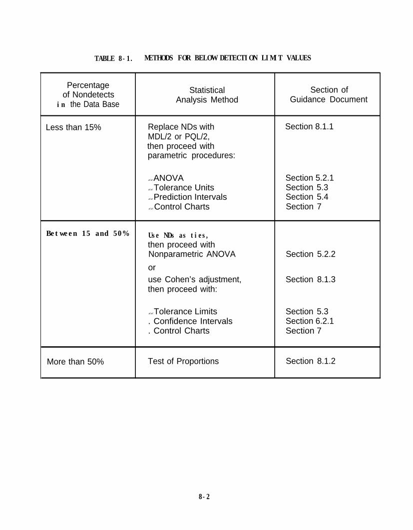
TABLE 8-1. METHODS FOR BELOW DETECTION LIMIT VALUES

Percentageof Nondetects

in the Data Base

Statistical Section ofAnalysis Method Guidance Document

Less than 15% Replace NDs withMDL/2 or PQL/2,then proceed withparametric procedures:

Section 8.1.1

??ANOVA Section 5.2.1??Tolerance Units Section 5.3??Prediction Intervals Section 5.4??Control Charts Section 7

Between 15 and 50% Use NDs as ties,then proceed withNonparametric ANOVA Section 5.2.2oruse Cohen’s adjustment, Section 8.1.3then proceed with:

More than 50%

??Tolerance Limits. Confidence Intervals. Control Charts

Test of Proportions

Section 5.3Section 6.2.1Section 7

Section 8.1.2

8-2

It should be noted that the nonparametric methods presented earlier auto-matically deal with values below detection by regarding them as all tied at alevel below any quantitated results. The nonparametric methods may be used ifthere is a Moderate amount of data below detection. If the proportion of non-quantified values in the data exceeds 25%, these methods should be used withcaution. They should probably not be used if less than half of the data con-sists of quantified concentrations.

8.1.1 The DL/2 Method

The amount of data that are below detection plays an important role inselecting the method to deal with the limit of detection problem. If a smallproportion of the observations are not detected, these may be replaced with asmall number, usually the method detection limit divided by 2 (MDL/2), and theusual analysis performed. This is the recommended method for use with theanalysis of various procedure of Section 5.2.1. Seek professional help if indoubt about dealing with values below detection limit. The-results of theanalysis are generally not sensitive to the specific choice of the replacementnumber.

As a guideline, if 15% or fewer of the values are not detected, replacethem with the method detection limit divided by two and proceed with theappropriate analysis using these modified values. Practical quantitationlimits (PQL) for Appendix IX compounds were published by EPA in the FederalRegister (Vol 52, No 131, July 9, 1987, pp 25947-25952). These give practicalquantitation limits by compound and analytical method that may be used inreplacing a small amount of nondetected data with the quantitation limitdivided by 2. If approved by the Regional Administrator, site specific PQL'smay be used in this procedure. If more than 15% of the values are reported asnot detected, it is preferable to use a nonparametric method or a test of pro-portions.

8.1.2. Test of Proportions

If more than 50% of the data are below detection but at least lO%.of theobservations are quantified, a test of proportions may be used to compare thebackground well data with the compliance well data. Clearly, if none of thebackground well observations were above the detection limit, but all of thecompliance well observations were above the detection limit, one would suspectcontamination. In general the difference may not be as obvious. However, ahigher proportion of quantitated values in compliance wells could provide evi-dence of contamination. The test of proportions is a method to determinewhether a difference in proportion of detected values in the background wellobservations and compliance well observations provides statistically signifi-cant evidence of contamination.

The test of proportions should be used when the proportion of quantifiedvalues is small to moderate (i.e., between 10% and 50%). If very few quanti-fied values are found, a method based on the Poisson distribution may be usedas an alternative approach. A method based on a tolerance limit for thenumber of detected compounds and the maximum concentration found for anydetected compound has been proposed by Gibbons (1988). This alternative would

8-3

be appropriate when the number of detected compounds is quite small relativeto the number of compounds analyzed for as might occur in detectionmonitoring.

PURPOSE

The test of proportions determines whether the proportion of compoundsdetected in the compliance well data differs significantly from the proportionof compounds detected in the background well data. If there is a significantdifference, this is statistically significant evidence of contamination.

PROCEDURE

The procedure uses the normal distribution approximation to the binomialdistribution.ally,

This assumes that the sample size is reasonably large. Gener-if the proportion of detected values is denoted by P, and the sample

size is n, then the normal approximation is adequate, provided that nP andn(l-P) both are greater than or equal to 5.

Step 1. Check criterion for using the normal approximation.

. Determine X, the number of background well samples in which thecompound was detected, and Y, the number of compliance well samplesin which the compound was detected.

. Let nb be the total number of background well samples analyzed andnc be the total number of compliance well samples analyzed. Letn = nb + nc.

.

Step 2.samples:

Compute the proportion of detects in the background well

Step 3.samples:

Compute the proportion of detects in the compliance well

Step 4. Compute the standard error of the difference in proportions:

{[(x+y)/(nb+nc)][1 - (X+Y)/(nb+nc)][1/nb + 1/nc]}½

and form the statistic:

8-4

Step 5. Compare the absolute value of Z to the 97.5th percentile fromthe standard normal distribution, 1.96. If the absolute value of Z exceeds1.96, this provides statistically significant evidence at the 5% significancelevel that the proportion of compliance well samples where the compound wasdetected exceeds the proportion of background well samples where the compoundwas detected. This would be interpreted as evidence of contamination. (Thetwo-sided test is used to provide information about differences in eitherdirection.)

EXAMPLE

Table 8-2 contains data on cadmium concentrations measured in backgroundwell and compliance wells at a facility. In the table, "BDL" is used forbelow detection limit.

Since both of these exceed 5, the normal approximation is justified.

Step 2. Estimate the proportion above detection in the backgroundwells. As shown in Table 8-2, there were 24 samples from background wellsanalyzed for cadmium, so nb = 24. Of these, 16 were below detection and X = 8were above detection, so Pb = 8/24 = 0.333.

Step 3. Estimate the proportion above detection in the compliancewells. There were 64 samples from compliance wells analyzed for cadmium, with40 below detection and 24 detected values. This gives nc = 64, Y = 24, so PC= 24/64 = 0.375.

Step 4. Calculate the standard error of the difference in proportions.

SD= ([(8+24)/(24+64)1[1-(8+24)/(24+64)](1/24 +l/64)}½ = 0.115

Step 5. Form the statistic Z and compare it to the normal distribution.

Z = 0.375 - 0.333 = 0 370.115

which is less in absolute value than the value from the normal distribution,1.96. Consequently, there is no statistically significant evidence that theproportion of samples with cadmium levels above the detection limit differs inthe background well and compliance well samples.

8-5

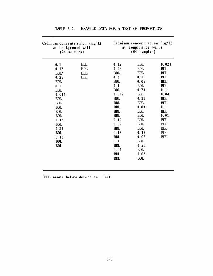
TABLE 8-2. EXAMPLE DATA FOR A TEST OF PROPORTIONS

Cadmium concentration (µg/L) Cadmium concentration (µg/L)at background well at compliance wells

(24 samples) (64 samples)

0.10.12BDL*0.26BDL0.1BDL0.014BDLBDLBDLBDLBDL0.12BDL0.21BDL0.12BDLBDL

BDL 0.12BDL 0.08BDL BDLBDL 0.2

BDL0.1BDL0.012BDLBDLBDLBDLBDL0.120.07BDL0.19BDL0.1BDL0.01BDLBDL

BDLBDLBDL0.110.06BDL0.23BDL0.11BDL0.031BDLBDLBDLBDLBDL0.120.08BDL0.26BDL0.02BDL

0.024BDLBDLBDLBDLBDL0.10.04BDLBDL0.1BDL0.01BDLBDLBDLBDLBDL

*BDL means below detection limit.

8-6

INTERPRETATION

Since the proportion of water samples with detected amounts of cadmium inthe compliance wells was not significantly different from that in thebackground wells, the data are interpreted to provide no evidence of contam-ination. Had the proportion of samples with detectable levels of cadmium inthe compliance wells been significantly higher than that in the backgroundwells this would have been evidence of contamination. Had the proportion beensignificantly higher in the background wells, additional study would have beenrequired. This could indicate that contamination was migrating from an off-site source, or it could mean that the hydraulic gradient had been incorrectlyestimated or had changed and that contamination was occurring from the facil-ity, but the ground-water flow was not in the direction originally esti-mated. Mounding of contaminants in the ground water near the background wellscould also be a possible explanation of this observance.

8.1.3 Cohen's Method

If a confidence interval or a tolerance interval based upon the normaldistribution is being constructed, a technique presented by Cohen (1959)specifies a method to adjust the sample mean and sample standard deviation toaccount for data below the detection limit. The only requirements for the useof this technique is that the data are normally distributed and that thedetection limit be always the same. This technique is demonstrated below.

PURPOSE

Cohen's method provides estimates of the sample mean and standard devia-tion when some ( < 50%) observations are below detection. These estimates canthen be used to construct tolerance, confidence, or prediction intervals.

PROCEDURE

Let n be the total number of observations, m represent the number of datapoints above the detection limit (DL), and Xi represent the value of the ithconstituent value above the detection limit.

8-7

where n is the total number of observations (i.e.., above and below thedetection limit), and where DL is equal to the detection limit.

Step 4. Estimate the corrected sample mean, which accounts for the databelow detection limit, as follows:

Step 5. Estimate the corrected sample standard deviation, which accountsfor the data below detection limit, as follows:

EXAMPLE

Table 8-3 contains data on sulfate concentrations. Three observations ofthe 24 were below the detection limit of 1,450 mg/L and are denoted by"< 1,450" in the table.

Step 1. Calculate the mean from the m = 21 values above detection

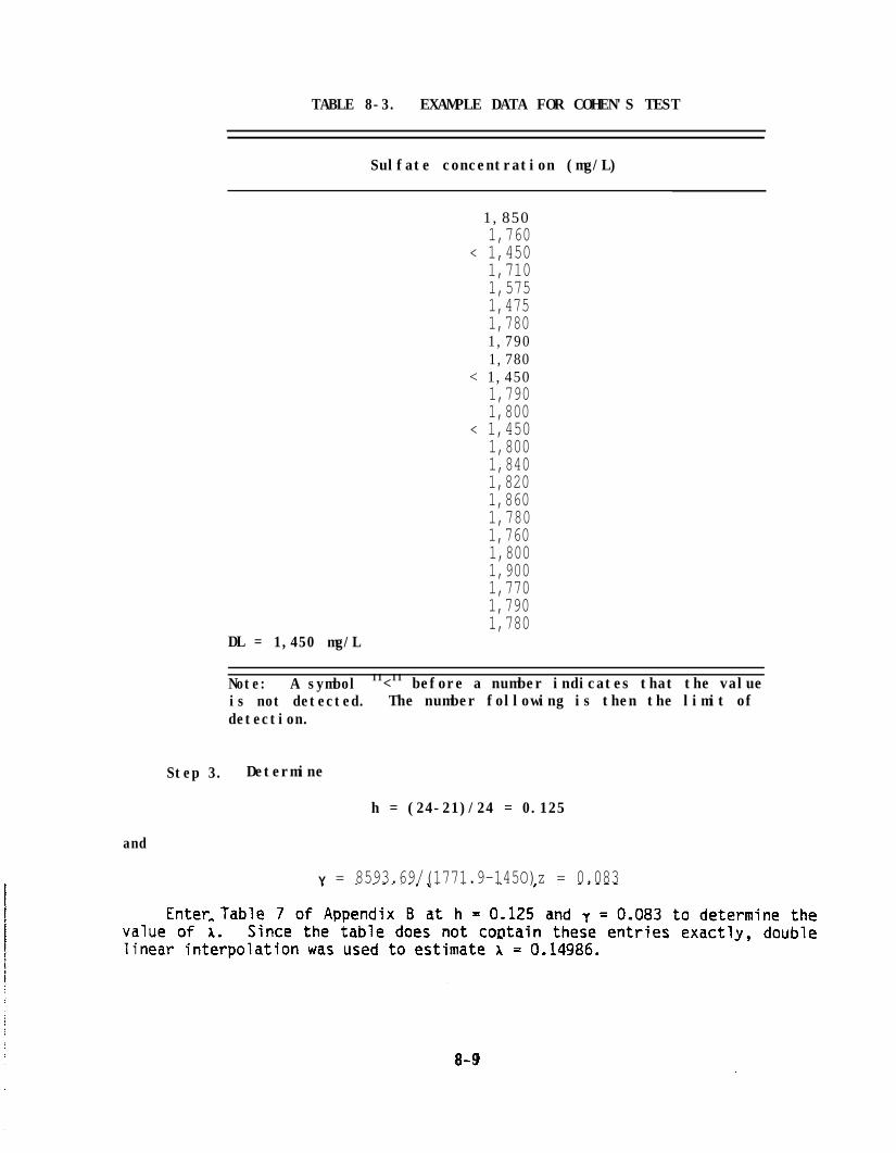
TABLE 8-3. EXAMPLE DATA FOR COHEN'S TEST

Sulfate concentration (mg/L)

1,8501,760

< 1,4501,7101,5751,4751,7801,7901,780

< 1,4501,7901,800

< 1,4501,8001,8401,8201,8601,7801,7601,8001,9001,7701,7901,780

DL = 1,450 mg/L

Note: A symbol 11<11 before a number indicates that the valueis not detected. The number following is then the limit ofdetection.

Step 3. Determine

h = (24-21)/24 = 0.125

and

Y = 8593.69/(1771.9-145O)z = 0.083

8-9

For the interested reader, the details of the double linear interpolationre provided.

The values from Table 7 between which the user needs to interpolate are:

Y h = 0.10 h = 0.15

0.05 0.11431 0.179350.10 0.11804 0.18479

There are 0.025 units between 0.01 and 0.125 on the h-scale. There are0.05 units between 0.10 and 0.15. Therefore, the value of interest (0.125)lies (0.025/0.05 * 100) = 50% of the distance along the interval between 0.10and 0.15. To linearly interpolate between the tabulated values on the h axis,the range between the values must be calculated, the value that is 50% of thedistance along the range must be computed and then that value must be added tothe lower point on the tabulated values. The result is the interpolatedvalue. The interpolated points on the h-scale for the current example are:

0.17935 - 0.11431 = 0.06504 0.06504 * 0.50 = 0.032520.11431 + 0.03252 = 0.14683

0.18479 - 0.11804 = 0.06675 0.06675 * 0.50 = 0.0333750.11804 + 0.033375 = 0.151415

On the y-axis there are 0.033 units between 0.05 and 0.083. There are0.05 units between 0.05 and 0.10. The value of interest (0.083) lies(0.0330.05 * 100) = 66% of the distance along the interval between 0.05 and0.10. The interpolated point on the y-axis is:

0.141415 - 0.14683 = 0.004585 0.004585 * 0.66 = 0.00302610.14683 + 0.0030261 = 0.14986

Step 6. These modified estimates of the mean, x = 1723.66, and of thestandard deviation, S = 155.31, would be used in the tolerance or confidenceinterval procedure. For example, if the sulfate concentrations representbackground at a facility, the upper 95% tolerance limit becomes

1723.7 + (155.3)(2.309) = 2082.3 mg/L

8-10

For the interested reader, the details of the double linear interpolationre provided.

The values from Table 7 between which the user needs to interpolate are:

Y h = 0.10 h = 0.15

0.05 0.11431 0.179350.10 0.11804 0.18479

There are 0.025 units between 0.01 and 0.125 on the h-scale. There are0.05 units between 0.10 and 0.15. Therefore, the value of interest (0.125)lies (0.025/0.05 * 100) = 50% of the distance along the interval between 0.10and 0.15. To linearly interpolate between the tabulated values on the h axis,the range between the values must be calculated, the value that is 50% of thedistance along the range must be computed and then that value must be added tothe lower point on the tabulated values. The result is the interpolatedvalue. The interpolated points on the h-scale for the current example are:

0.17935 - 0.11431 = 0.06504 0.06504 * 0.50 = 0.032520.11431 + 0.03252 = 0.14683

0.18479 - 0.11804 = 0.06675 0.06675 * 0.50 = 0.0333750.11804 + 0.033375 = 0.151415

On the y-axis there are 0.033 units between 0.05 and 0.083. There are0.05 units between 0.05 and 0.10. The value of interest (0.083) lies(0.0330.05 * 100) = 66% of the distance along the interval between 0.05 and0.10. The interpolated point on the y-axis is:

0.141415 - 0.14683 = 0.004585 0.004585 * 0.66 = 0.00302610.14683 + 0.0030261 = 0.14986

Step 6. These modified estimates of the mean, x = 1723.66, and of thestandard deviation, S = 155.31, would be used in the tolerance or confidenceinterval procedure. For example, if the sulfate concentrations representbackground at a facility, the upper 95% tolerance limit becomes

1723.7 + (155.3)(2.309) = 2082.3 mg/L

8-10

Observations from compliance wells in excess of 2,082 mg/L would give sta-tistically significant evidence of contamination.

INTERPRETATION

Cohen's method provides maximum likelihood estimates of the mean andvariance of a censored normal distribution. That is, of observations thatfollow a normal distribution except for those below a limit of detection,which are reported as "not detected." The modified estimates reflect the factthat the not detected observations are below the limit of detection, but notnecessarily zero. The large sample properties of the modified estimates allowfor them to be used with the normal theory procedures as a means of adjustingfor not detected values in the data. Use of Cohen's method in more compli-cated calculations such as those required for analysis of variance procedures,requires special consideration from a professional statistician.

8.2 OUTLIERS

A ground-water constituent concentration value that is much differentfrom most other values in a data set for the same ground-water constituentconcentration can be referred to as an "outlier." Possible reasons foroutliers can be:

. A catastrophic unnatural occurrence such as a spill;

. Inconsistent sampling or analytical chemistry methodology that mayresult in laboratory contamination or other anomalies;

. Errors in the transcription of data values or decimal points; and

. True but extreme ground-water constituent concentration measure-ments.

There are several tests to determine if there is statistical evidencethat an observation is an outlier. The reference for the test presented hereis ASTM paper E178-75.

PURPOSE

The purpose of a test for outliers is to determine whether there isstatistical evidence that an observation that appears extreme does not fit thedistribution of the rest of the data. If a suspect observation is identifiedas an outlier, then steps need to be taken to determine whether it is theresult of an error or a valid extreme observation.

PROCEDURE

Let the sample of observations of a hazardous constituent of ground waterbe denoted by Xi, . . . , Xn. For specificity, assume that the data have beenordered and that the largest observation, denoted by Xn, is suspected of beingan outlier. Generally, inspection of the data suggests values that do not

8-11

appear to belong to the data set. For example, if the largest observation isan order of magnitude larger than the other observations, it would be suspect.

including all observations.

Step 2. Form the statistic, Tn:

Note that T is the difference between the largest observation and the samplemean, divided by the sample standard deviation.

step 3. Compare the statistic Tn to the critical value given the samplesize, n, in Table 8 in Appendix B. If the Tn statistic exceeds the critical

value from the table, this is evidence that the suspect observation, Xn, is astatistical outlier.

Step 4. If the value is identified as an outlier, one of the actionsoutlined below should be taken. (The appropriate action depends on what canbe learned about the observation.) The records of the sampling and analysisof the sample that led to it should be investigated to determine whether theoutlier resulted from an error that can be identified.

. If an error (in transcription, dilution, analytical procedure, etc.)can be identified and the correct value recovered, the observation should bereplaced by its corrected value and the appropriate statistical analysis donewith the corrected value.

. If it can be determined that the observation is in error, but thecorrect value cannot be determined, then the observation should be deletedfrom the data set and the appropriate statistical analysis performed. Thefact that the observation was deleted and the reason for its deletion shouldbe reported when reporting the results of the statistical analysis.

• If no error in the value can be documented then it must be assumedthat the observation is a true but extreme value. In this case it must not bealtered. It may be desirable to obtain another sample to confirm the observa-tion. However, analysis and reporting should retain the observation and statethat no error was found in tracing the sample that led to the extreme observa-tion.

EXAMPLE

Table 8-4 contains 19 values of total organic carbon (TOC) that wereobtained from a monitoring well. Inspection shows one value which at 11,000mg/L is nearly an order of magnitude larger than most of the other observa-tions. It is a suspected outlier.

8-12

TABLE 8-4. EXAMPLE DATA FOR TESTING FOR AN OUTLIER

Total organic carbon (mg/L)

1,7001,9001,5001,300

11,0001,2501,0001,3001,2001,4501,0001,3001,0002,2004,9003,7001,6002,5001,900

Step 2. Calculate the statistic T19.

T19 = (llOOO-2300)/2325.9 = 3.74

Step 3. Referring to Table 8 of Appendix B for the upper 5% significancelevel, with n = 19, the critical value is 2.532. Since the value of the. statistic T19 = 3.74 is greater than 2.532, there is statistical evidencethat the largest observation is an outlier.

Step 4. In this case, tracking the data revealed that the unusual valueof 11,000 resulted from a keying error and that the correct value was 1,100.This correction was then made in the data.

INTERPRETATION

An observation that is 4 or 5 times as large as the rest of the data isgenerally viewed with suspicion. An observation that is an order of magnitudedifferent could arise by a common error of misplacing a decimal. The test foran outlier provides a statistical basis for determining whether an observation

8-13

is statistically different from the rest of the data. If it is, then it is astatistical outlier. However, a statistical outlier may not be dropped oraltered just because it has been identified as an outlier. The test providesformal identification of an observation as an outlier, but does not identify

the cause of the difference.

Whether or not a statistical test is done, any suspect data point shouldbe checked. An observation may be corrected or dropped only if it can bedetermined that an error has occurred. If the error can be identified andcorrected (as in transcription or keying) the correction should be made andthe corrected values used. A value that is demonstrated to be incorrect maybe deleted from the data. However, if no specific error can be documented,the observation must be retained in the data. Identification of an observa-tion as an outlier but with no error documented could be used to suggestresampling to confirm the value.

8-14

APPENDIX A

GENERAL STATISTICAL CONSIDERATIONS ANDGLOSSARY OF STATISTICAL TERMS

A-l

GENERAL STATISTICAL CONSIDERATIONS

FALSE ALARMS OR TYPE I ERRORS

The statistical analysis of data from ground-water monitoring at RCRAsites has as its goal the determination of whether the data provide evidenceof the presence of, or an increase in the level of contamination. In the caseof detection monitoring, the goal of the statistical analysis is to determinewhether statistically significant evidence of contamination exists. In thecase of compliance monitoring, the goal is to determine whether statisticallysignificant evidence of concentration levels exceeding compliance limitsexists. In monitoring sites in corrective action, the goal is to determinewhether levels of the hazardous constituents are still above compliance limitsor have been reduced to, at, or below the compliance limit.

These questions are addressed by the use of hypothesis tests. In thecase of detection monitoring, it is hypothesized that a site is not contami-nated; that is, the hazardous constituents are not present in the groundwater. Samples of the ground water are taken and analyzed for the constitu-ents in question. A hypothesis test is used to decide whether the data indi-cate the presence of the hazardous constituent. The test consists of calcu-lating one or more statistics from the data and comparing the calculatedresults to some prespecified critical levels.

In performing a statistical test, there are four possible outcomes. Twoof the possible outcomes result in the correct decision: (a) the test maycorrectly indicate that no contamination is present or (b) the test may cor-rectly indicate the presence of contamination. The other two possibilitiesare errors: (c) the test may indicate that contamination is present when infact it is not or (d) the test may fail to detect contamination when it ispresent.

If the stated hypothesis is that no contamination is present (usuallycalled the null hypothesis) and the test indicates that contamination ispresent when in fact it is not, this is called a Type I error. Statisticalhypothesis tests are generally set up to control the probability of Type Ierror to be no more than a specified value, called the significance level, andusually denoted by a. Thus in detection monitoring, the null hypothesis wouldbe that the level of each hazardous constituent is zero (or at least belowdetection). The test would reject this hypothesis if some measure of concen-tration were too large, indicating contamination. A Type I error would be afalse alarm or a triggering event that is inappropriate.

In compliance monitoring, the null hypothesis is that the level of eachhazardous constituent is less than or equal to the appropriate compliance

A-3

limit. For the purpose of setting up the statistical procedure, the simplenull hypothesis that the level is equal to the compliance limit would beAs in detection monitoring, the test would indicate contamination if

some measure of concentration is too large. A false alarm or Type I errorwould occur if the statistical procedure indicated that levels exceed the

appropriate compliance limits when, in fact, they do not. Such an error wouldbe a false alarm in that it would indicate falsely that compliance limits were

being exceeded.

PROBILITY OF DETECTION AND TYPE II ERROR

The other type of error that can occur is called a Type II error. Itoccurs if the test fails to detect contamination that is present. Thus aType II error is a missed detection. While the probability of a Type I errorcan be specified, since it is the probability that the test will give a falsealarm, the probability of a Type II error depends on several factors, includ-ing the statistical test, the sample size, and the significance level or prob-ability of Type I error. In addition, it depends on the degree of contamina-tion present. In general, the probability of a Type II error decreases as thelevel of contamination increases. Thus a test may be likely to miss low lev-els of contamination, less likely to miss moderate contamination, and veryunlikely to miss high levels of contamination.

One can discuss the probability of a Type II error as the probability ofa missed detection, or one can discuss the complement (one minus the prob-ability of Type II error) of this probability. The complement, or probabilityof detection, is also called the power of the test. It depends on the magni-tude of the contamination so that the power or probability of detecting con-tamination increases with the degree of contamination.

If the probability of a Type I error is specified, then for a given sta-tistical test, the power depends on the sample size and the alternative ofinterest. In order to specify a desired power or probability of detection,one must specify the alternative that should be detected. Since generally thepower will increase as the alternative differs more and more from the nullhypothesis, one usually tries to specify the alternative that is closest tothe null hypothesis, yet enough different that it is important to detect.

In the detection monitoring situation, the null hypothesis is that theconcentration of the hazardous constituent is zero (or at least below detec-tion). In this case the alternative of interest is that there is a concen-tration of the hazardous constituent that is above the detection limit and islarge enough so that the monitoring procedure should detect it. Since it is avery difficult problem to select a concentration of each hazardous constituentthat should be detectable with specified power, a more useful approach is todetermine the power of a test at several alternatives and decide whether theprocedure is acceptable on the basis of this power function rather than on thepower against a single alternative.

In order to increase the power, a larger sample must be taken. Thiswould mean sampling at more frequent intervals. There is a limit to how muchcan be achieved, however. In cases with limited water flow, it may not bepossible to sample wells as frequently as desired. If samples close together

A-4

in time prove to be correlated, this correlation reduces the informationavailable from the different samples. The additional cost of sampling andanalysis will also impose practical limitations on the sample size that can beused.

Additional wells could also be used to increase the performance of thetest. The additional monitoring wells would primarily be helpful in ensuringthat a plume would not escape detection by missing the monitoring wells. How-ever, in some situations the additional wells would contribute to a largersample size and so improve the power.

In compliance monitoring the emphasis is on determining whether addi-tional contamination has occurred, raising the concentration above a compli-ance limit. If the compliance limit is determined from the background welllevels, the null hypothesis is that the difference between the background andcompliance well concentrations is zero. The alternative of interest is thatthe compliance well concentration exceeds the background concentration. Thissituation is essentially the same for power considerations as that of thedetection monitoring situation.

If compliance monitoring is relative to a compliance limit (MCL or ACL),specified as a constant, then the situation is different. Here the null hypo-thesis is that the concentration is less than or equal to the compliancelimit, with equality used to establish the test. The alternative is that theconcentration is above the compliance limit. In order to specify power, aminimum amount above the compliance limit must be established and power speci-fied for that alternative or the power function evaluated for several possiblealternatives.

SAMPLE DESIGNS AND ASSUMPTIONS

As discussed in Section 2, the sample design to be employed at a regu-lated unit will primarily depend on the hydrogeologic evaluation of thesite. Wells should be sited to provide multiple background wells hydrauli-cally upgradient from the regulated unit. The background wells allow fordetermination of natural spatial variability in ground-water quality. Theyalso allow for estimation of background levels with greater precision thanwould be possible from a single upgradient well. Compliance wells should besited hydraulically downgradient to each regulated unit. The location andspacing of the wells, as well as the depth of sampling, would be determinedfrom the hydrogeology to ensure that at least one of the wells should inter-cept a plume of contamination of reasonable size.

Thus the assumed sample design is for a sample of wells to include anumber of background wells for the site, together with a number of compliancewells for each regulated unit at the site. In the event that a site has onlya single regulated unit, there would be two groups of wells, background andcompliance. If a site has multiple regulated units, there would be a set ofcompliance wells for each regulated unit, allowing for detection monitoring orcompliance monitoring separately at each regulated unit.

Data from the analysis of the water at each well are initially assumed tofollow a normal distribution. This is likely to be the case for detection

A-5

monitoring of analytes in that levels should be near zero and errors wouldlikely represent instrument or other sampling and analysis variability. Ifcontamination is present, then the distribution of the data may be skewed tothe right, giving a few very large values. The assumption of normality oferrors in the detection monitoring case is quite reasonable, with deviationsfrom normality likely indicating some degree of contamination. Tests of nor-mality are recommended to ensure that the data are adequately represented bythe normal distribution.

In the compliance monitoring case, the data for each analyte will againinitially be assumed to follow the normal distribution. In this case, how-ever, since there is a nonzero concentration of the analyte in the groundwater, normality is more of an issue. Tests of normality are recommended. Ifevidence of nonnormality is found, the data should be transformed or adistribution-free test be used to determine whether statistically significantevidence of contamination exists.

The standard situation would result in multiple samples (taken at dif-ferent times) of water from each well. The wells would form groups of back-ground wells and compliance wells for each regulated unit. The statisticalprocedures recommended would allow for testing each compliance well groupagainst the background group. Further, tests among the compliance wellswithin a group are recommended to determine whether a single well might beintercepting an isolated plume. The specific procedures discussed and recom-mended in the preceding sections should cover the majority of cases. They didnot cover all of the possibilities. In the event that none of the proceduresdescribed and illustrated appears to apply to a particular case at a givenregulated site, consultation with a statistician should be sought to determinean appropriate statistical procedure.

The following approach is recommended. If a regulated unit is in detec-tion monitoring, it will remain in detection monitoring until or unless thereis statistically significant evidence of contamination, in which case it wouldbe placed in compliance monitoring. Likewise, if a regulated unit is in com-pliance monitoring, it will remain in compliance monitoring unless or untilthere is statistically significant evidence of further contamination, in whichcase it would move into corrective action.

In monitoring a regulated unit with multiple compliance wells, two typesof significance levels are considered. One is an experimentwise significancelevel and the other is a comparisonwise significance level. When a proceduresuch as analysis of variance is used that considers several compliance wellssimultaneously, the significance is an experimentwise significance. Ifindividual well comparisons are made, each of those comparisons is done at acomparisonwise significance level.

The fact that many comparisons will be made at a regulated unit withmultiple compliance wells can make the probability that at least one of thecomparisons will be incorrectly significant too high. To control the falsepositive rate, multiple comparisons procedures are allowed that control theexperimentwise significance level to be 5%. That is, the probability that one

more of the comparisons will falsely indicate contamination is controlled

A-6

at 5%. However, to provide some assurance of adequate power to detect realcontamination, the comparisonwise significance level for comparing eachindividual well to the background is required to be no less than 1%.

Control of the experimentwise significance level via multiple comparisonsprocedures is allowed for comparisons among several wells. However, use of anexperimentwise significance level for the comparisons among the different haz-ardous constituents is not permitted. Each hazardous constituent to be moni-tored for in the permit must be treated separately.

A-7

GLOSSARY OF STATISTICAL TERMS(underlined terms are explained subsequently)

Alpha (a)

Alpha-error

Alternative hypothesis

Arithmetic average

Autocorrelation

Biased estimator

Bonferroni t

A greek letter used to denote the significancelevel or probability of a Type I error.

Sometimes used for Type I error.

An alternative hypothesis specifies that theunderlying distribution differs from the nullhypothesis. The alternative hypothesis usuallyspecifies the value of a parameter, for examplethe mean concentration, that one is trying todetect.

The arithmetic average of a set of observationsis their sum divided by the number ofobservations.

This is a measure of dependence among sequentialobservations from the same well. There are dif-ferent orders of autocorrelation, depending onhow far apart in time the correlation per-sists. For example, the first order auto-correlation is the correlation between suc-cessive pairs of observations.

A biased estimator is an estimator that has anexpectation or average value that is not equalto the parameter it is estimating. Often thebias decreases as the sample size increases.

This is an approach, developed by Bonferroni, tocontrol the experimentwise error rate in multi-ple comparisons. The number of comparisons orhypotheses to be tested is fixed (at k) and a"t" statistic is computed to test each ofthese. Instead of the usual "t" table, whereeach of these tests would be done at the sig-nificance level alpha, a special table is usedso that each test is done at level aloha/k.This ensures that the experimentwise error rateis no more than alpha.

A-8

Comparisonwise error rate This term is used in association with multiplecomparisons. It refers to the probability of anerror occurring on a single comparison of sev-eral that might be done. It is computed assum-ing that the single comparison or hypothesistest is the only one being done.

Composite hypothesis This is a hypothesis for which not all relevantparameters are specified. A composite hypothe-sis is made up of two or more simple hypothe-ses. For example, the hypothesis that the dataare normally distributed with unspecified meanand variance is a composite hypothesis.

Confidence coefficient The confidence coefficient of a confidenceinterval for a parameter is the probability thatthe random interval constructed from the sampledata contains the true value of the parameter.The confidence coefficient is related to thesignificance level of an associated hypothesistest by the fact that the significance level (inpercent) is one hundred minus the confidencecoefficient (in percent).

Confidence interval A confidence interval for a parameter is arandom interval constructed from sample data insuch a way that the probability that theinterval will contain the true value of theparameter is a specified value.

Cumulative distributionfunction

The distribution function for a random variable,X, is a function that specifies the probabilitythat X is less than or equal to t, for all realvalues of t.

Distribution-free

Distribution function

Estimator

This is sometimes used as a synonym fornonparametric. A statistic is distribution-freeif its distribution does not depend upon whichspecific distribution function (in a largeclass) the observations follow.

This document uses "Cumulative DistributionFunction" and "Distribution Function" inter-changeably. See Cumulative DistributionFunction.

An estimator is a statistic computed from theobserved data. It is used to estimate a param-eter of interest; for example, the populationmean. Often estimators are the sample equiva-lents of the population parameters.

A-9

Experimentwise error rate This term refers to multiple comparisons. If atotal of n decisions are made about comparisons(for example of compliance wells to backgroundwells) and x of the decisions are wrong, thenthe experimentwise error rate is x/n. Theprobability that X exceeds zero is the experi-mentwise significance.

Hypothesis

Independence

Mean

Median

Multiple comparisonprocedure

This is a formal statement about a parameter ofinterest and the distribution of a statistic.It is usually used as a null hypothesis or analternative hypothesis. For example, the nullhypothesis might specify that ground water had azero concentration of benzene and that analyti-cal errors followed a normal distribution withmean zero and standard deviation 1 ppm.

A set of events are independent if theprobability of the joint occurrence of anysubset of the events factors into the product ofthe probabilities of the events. A set ofobservations is independent if the jointdistribution function of the random errorsassociated with the observations factors intothe product of the distribution functions.

Arithmetic average.

This is the middle value of a sample when theobservations have been ordered from least togreatest. If the number of observations is odd,it is the middle observation. If the number ofobservations is even, it is customary to takethe midpoint between the two middle observa-tions. For a distribution, the median is avalue such that the probability is one-half thatan observation will fall above or below themedian.

This is a statistical procedure that makes alarge number of decisions or comparisons on oneset of data. For example, at a sampling period,several compliance well concentrations may becompared to the background well concentration.

Nonparametric statistical A nonparametric statistical procedure is aprocedure statistical procedure that has desirable

properties that hold under mild assumptionsregarding the data. Typically the procedure isvalid for a large class of distributions ratherthan for a specific distribution of the datasuch as the normal.

A-10

Normal population,normality

Null hypothesis

One-sided test

The errors associated with the observationsfollow the normal or Gaussian distributionfunction.

A null hypothesis specifies the underlyingdistribution of the data completely. Often thenull distribution specifies that there is nodifference between the mean concentration inbackground well water samples and compliancewell water samples. Typically, the null hypo-thesis is a simple hypothesis.

A one-sided test is appropriate if concentra-tions higher than those specified by the nullhypothesis are of concern. A one-sided testonly rejects for differences that are large andin a prespecified direction.

One-sided tolerance limit This is an upper limit on observations from aspecified distribution.

One-sided confidence limit This is an upper limit on a parameter of adistribution.

Order statistics The sample values observed after they have beenarranged in increasing order.

Outlier An outlier is an observation that is found tolie an unusually long way from the rest of theobservations in a series of replicateobservations.

Parameter A parameter is an unknown constant associatedwith a population. For example, the meanconcentration of a hazardous constituent inground water is a parameter of interest.

Percentile A percentile of a distribution is a value belowwhich a specified proportion or percent of theobservations from that distribution will fall.

Post hoc comparison

Power

This is a comparison, say between hazardousconstituent concentrations in two wells, thatwas found to be of interest after the data werecollected. Special methods must be used todetermine significance levels for post hoccomparisons.

The power of a test is the probability that thetest will reject under a specified alternativehypothesis. This is one minus the probabilityof a Type II error. The power is a measure of

A-11

the test's ability to detect a difference ofspecified size from the null hypothesis.

Sample standard deviation This is the square root of the sample variance.

Sample variance This is a statistic (computed on a sample ofobservations rather than on the whole popula-tion) that measures the variability or spread ofthe observations about the sample mean. It isthe sum of the squared differences from thesample mean, divided by the number of observa-tions less one.

Serial correlation This is the correlation of observations spaced aconstant interval apart in a series. For exam-ple, the first order serial correlation is thecorrelation between adjacent observations. Thefirst order serial correlation is found by cor-relating the pairs consisting of the first andsecond, second and third, third and fourth,etc., observations.

Significance level Sometimes referred to as the alpha level, thesignificance level of a test is the probabilityof falsely rejecting a true null hypothesis.The probability of a Type I error.

Simple hypothesis A hypothesis which completely specifies thedistribution of the observed random variables.To completely define a distribution, both thetype of distribution and numeric values for theparameters must be given.

Test statistic A test statistic is a value computed from theobserved data. This value is used to test ahypothesis by relating the value to a distribu-tion table and rejecting the hypothesis if thecomputed value falls in a region that has lowprobability under the hypothesis being tested.A "t" statistic, an "F" statistic, and a chi-squared statistic are examples.

Trend analysis This refers to a collection of statisticalmethods that analyze data to determine trendsover time. The trends may be of various types,steady increases (or decreases), or a stepincrease at a point in time.

Type I error A Type I error occurs when a true nullhypothesis is rejected erroneously. In themonitoring context a Type I error occurs when a

A-12

Type II error

Unbiased estimator

test incorrectly indicates contamination or anincrease in contamination at a regulated unit.

A Type II error occurs when one fails to rejecta null hypothesis that is false. In the moni-toring context, a Type II error occurs whenmonitoring fails to detect contamination or anincrease in a concentration of a hazardousconstituent.

An unbiased estimator is an estimator that haszero bias. That is, its expectation is equal tothe parameter it is estimating. Its averagevalue is the parameter.

A-13

APPENDIX B

STATISTICAL TABLES

B-1

1

2

3

4

5

6

7

8

B-3

SOURCE: Johnson, Norman L. and F. C. Leone. 1977. Statistics and ExperimentalDesign in Engineering and the Physical Sciences. Vol. I. Second Edition. JohnWiley and Sons, New York.

B-4

TABLE 1. PERCENTILES OF THE x2 DISTRIBUTION WITHv DEGREES OF FREEDOM, x~,p

0

\p0.7050 0.900 0.950 0.9705 0.990 0.995 0.999

1/ \

1 1.323 2.706 3.841 05.024 6.635 7.879 10.832 2.773 4.605 '05.991 7.378 9.210 10.60 13.823 4.108 6.251 7.815 9.348 11.34 12.84 16.274 05.385 7.779 9.488 11.14 13.28 14.86 18.47

S 6.626 9.236 11.07 12.83 15.09 16.705 20.526 7.841 10.64 12.59 14.45 16.81 18..5.5 22.467 9.037 12.02 14.07 16.01 18.48 20.28 24.328 10.22 13.36 105.51 17..53 20.09 21.96 26.129 11.39 14.68 16.92 19.02 21.67 23.59 27.88

10 12..5.5 1.5.99 18.31 20.48 23.21 2.5.19 29..5911 13.70 17.28 19.68 2L92 24.72 26.76 31.2612 14.8.5 18..5S 21.03 23.34 26.22 28.30 32.9113 1.5.98 19.81 22.36 24.74 27.69 29.82 34.53l4 17.12 21.06 23.68 26.12 29.14- 31.32 36.12

15 18.25 21.31 2.5.00 27.49 30.58 32.80 37.7016 19.37 23.54 26.30 28.8.5 32.00 34.27 39.2517 20.49 24.77 27•.59 30.19 33.41 3.5.72 40.7918 21.60 25.99 28.87 31.53 34.81 37.16 42.3119 22.72 27.20 30.14 32.85 36.19 38..58 43.82

20 23.83 28.41 31.41 34.17 37..57 40.00 4.5.3221 24.93 29.62 32.67 35.48 38.93 41.40 46.8022 26.04 30.81 33.92 36.78 40.29 42.80 48.2723 27.14 32.01 3.5.17 38.08 41.64 44.18 49.7324 28.24 33.20 36.42 39.36 4:"98 405 ..56 .5US

2S 29.34 34.38 37.65 40.65 44.31 46.93 52.6226 30.43 3.5.56 38.89 41.92 45.64 48.29 54.0527 31.53 36.74 40.11 43.19 46.96 49.64 55.4828 32.62 37.92 41.34 44.46 48.28 50.99 56.8929 33.71 39.09 42..56 45.72 49.59 52.34 58.30

30 34.80 40.26 43.77 46.98 50.89 53.67 59.7040 45.62 51.80 55.76 59.34 63.69 66.77 73.4050 56.33 63.17 67.50 71.42 76.15 79.49 86.6660 66.98 74.40 79.08 83.30 88.38 91.95 99.61

70 n..58 805 ..53 90..53 95.02 100.4 104.2 112.380 88.13 96.58 101.9 106.6 112.3 116.3 124.890 98.65 107.6 113.1 118.1 124.1 128.3 137.2

100 109.1 118.5 124.3 129.6 135.8 140.2 149.4

NOTE: vl: Degrees of freedom for numeratorv 2 : Degrees of freedom for denominator

SOURCE: Johnson, Norman L. and F. C, Leone. 1977. Statistics and ExperimentalDesign in Engineering and the Physical Sciences. Vol. I. Second Edition. JohnWiley and Sons, New York.

B-5

2.13 2.782.02 2.571.94 2.451.90 2.371.86 2.311.83 2.261.01 2.231.75 2.131.73 2.091.70 2.041.65 1.96

3.202.902.742.632.552.502.452.322.272.212.13

3.51 3.753.17 3.372.97 3.142.83 3.002.74 2.902.67 2.822.61 2.762.47 2.602.40 2.532.34 2.462.24 2.33

B-6

TABLE 4. PERCENTILES OF THE STANDARD NORMAL DISTRIBUTION, Up

P 0.000 0.001 0.002 0.003 0.004 0.005 0.006 0.007 0.008 0.009

0.50 0.0000 0.0025 0.0050 0.0075 0.0100 0.0125 0.0 I500.51 0 .025 I 0.0276 0.0301 0.0326 0 .035 I 0.0376 0.04010.52 0.0502 0.0527 0.0552 0.0577 0.0602 0.0627 0.06520.53 0.0753 0.0778 0.0803. 0.0828 0.0853 0.0878 0.09040.54 0.1004 0.1030 0.1055 0.1080 0 . 1 O 5 0.1130 0.1156

0.55 0.1257 0.1282 0.1307 0. I332 0.1358 0. I 383 0.14080.56 0.1510 0.1535 0.1560 0.1586 0.1611 0.1637 0.16620.57 0.1764 0 . I 7 8 9 0.1815 0. I840 0.1866 0.1891 0.19170.58 0.2019 0.2045 0.2070 0.2096 0.2121 0.2147 0.21730.59 0.2275 0.2301 0.2327 0.2353 0.2378 0.2404 0.24300.60 0.2533 0.2559 0.2585 0 . 2 6 I I 0.2637 0.2663 0.26890.61 0.2793 0.2819 0.2845 0.2871 0.2898 0.2924 0.29500.62 0.3055 0.308I 0.3107 0.3134 0.3160 0.3186 0.32130.63 0.3319 0.3345 0.3372 0.3398 0.3425 0.3451 0.34780.64 0.3585 0.361 I 0.3638 0.3665 0.3692 0.3719 0.37450.65 0.3853 0.3880 0.3907 0.3934 0.3961 0.3989 0 . 4 0 I 60.66 0.4125 0.4152 0.4179 0.4207 0.4234 0.4261 0.42890.67 0.4399 0.4427 0.4454 0.4482 0.4510 0.4538 0.45650.68 0.4677 0.4705 0.4733 0.476 I 0.4789 0.4817 0.48450.69 0.4959 0.4987 0.5015 0.5044 0.5072 0.5101 0.5 I290.70 0.5244 0.5273 0.5302 0.5330 0.5359 0.5388 0.54170.71 0.5534 0.5563 0.5592 0.5622 0.565 1 0.568 1 0.57100.72 0.5828 0.5858 0.5888 0.5918 0.5948 0.5978 0.60080.73 0.6128 0.6158 0.6189 0.6219 0.6250 0.6280 0.63 I I0.74 0.6433 0.6464 0.6495 0.6526 0.6557 0.6588 0.6620

0.01750.04260.06770.0929O . l I S I0.14340.16870. I9420.21980.24560.27150.29760.32390.35050.37720.40430.43 I60.45930.48740.51580.54460.57400.60380.634 I0.665 I

0.020 1 0.02260.045 I 0.04760.0702 0.07250.0954 0.09790. I206 0.1’310.1459 0. I-1840.1713 0.17380. I968 0. I9930.2224 0.22500.2482 0.25080.274 I 0.27670.3002 0.30290.3266 0.32920.353 I 0.35580.3799 0.38260.4070 0.40970.4344 0.43720.4621 0.46490.4902 0.49300.5187 0.52IS0.5476 0.55050.5769 0.57990.6068 0.60980.6372 0.64030.6682 0.6713

NOTE: For values of P below 0.5, obtain the value of U(l-p) from Table 4 andchange its sign. For example, U0-45 = -U(l-0.45) = -U.0.55 = -0.1257.

(Continued)

B-7

TABLE 4 (Continued)

0.75 0.6745 0.67760.76 0.7063 0.70950.77 0.7388 0.74210.78 0.7722 0.77560.79 0.8064 0.80990.80 0.8416 0.84520.81 0.8779 0.88160.82 0.9154 0.91920.83 0.9542 0.958 I0.84 0.9945 0.9986O-85 I.0364 1.04070.86 1.0803 1.08480.87 1.1264 1.131I0.88 1.1750 1.18000.89 I.2265 I.23190.90 1.2816 1.28730.91 I.3408 1.34690.92 I .405 I 1.41180.93 I.4758 1 .48330.94 I ,5548 1.56320.95 1.6449 1.65460.96 1.7507 1.76240.97 1.8808 1.89570.98 2.0537 2.07490.99 2.3243 2.3656

0.68080.7 1 280.74540.77900.81340.84880.88530.92300.96211 .00271 .04501 .08931.13591.18501.2372

.2930

.3532

.4187

.49095 7 1 81.6666

I.77441.91 IO2.09692.4089

0.6840 0.6871 0.6903 0.69350.7160 0.7192 0.7225 0.72570.7488 0.7521 0.7544 0.75880.7824 0.7358 0.7892 0.79260 . 8 I 6 9 0.8204 0.8239 0.82740.8524 0.8560 0.8596 0.86330.8890 0.8927 0.8965 0.90020.9269 0.9307 0.9346 0.93850.9661 0 .970 I 0.974I 0.97821.0069 1.011O 1.0152 1.01941.0494 1.0537 I .058 I 1.0625I.0939 I.0985 1.1031 1.10771.1407 1.1455 I.1503 1.15521.1901 1.1952 I .2OO4 I.20551.2426 1 .2481 I.2536 1.25911.2988 1.3047 1.3106 I.31651.3595 1.3658 1.3722 I.37871.4255 1.4325 I.4395 1.44661.4985 1,5O63 l.5141 I.52201.5805 1.5893 I.5982 I .60721.6747 1.6849 1.6954 I .70601.7866 1.7991 I .8119 I .8250I.9268 1.9431 I.9600 I.97742.1201 2.1444 2.1701 2.19732.4573 2,5l21 2.5758 2.652I

0.69670.72900.76210.79610.83100.86690.90400.9424

I .3225I .3852I .45381.53011.61641.71691.8384I.99542.22622.7478

0.69990.73230.76550.79950.83450.87050.90780.94630.9863I.0279I.0714I.1 1701.16501.21601.2702I.32851.3917I.4611I.53821.6258I.7279I . 8 2 22.01412.257I2.8782

0.703I0.73560.76880.80300.838I0.87420.91160.95020.9904

.0322

.0758

.I217

. I 7 0 0-2212.2759

1.33461.39841.46841.54641.63521.73921.86632.03352.29043.0902

SOURCE: Johnson, Norman L. and F. C. Leone. 1977. Statistics and ExperimentaZDesign in Engineering and the Physical Sciences. Vol. I, Second Edition. JohnWiley and Sons, New York.

B-8

TABLE 5. TOLERANCE FACTORS (K) FOR ONE-SIDED NORMAL TOLERANCEINTERVALS WITH PROBABILITY LEVEL (CONFIDENCE FACTOR)

Y = 0.95 AND COVERAGE P = 95%

B-9

TABLE 6. PERCENTILES OF STUDENT's t-DISTRIBUTION

(F=l-a; n = degrees of freedom)

SOURCE: CRC Handbook of Tables for Probability and Statistics. 1966.W. H. Beyer, Editor. Published by the Chemical Rubber Company. Cleveland,Ohio.

B-10

ADJUSTING FOR NONDETECTED VALUES

SOURCE: Cohen, A. C., Jr. 1961. "Tables for Maximum Likelihood Estimates:Singly Truncated and Singly Censored Samples." Technometrics.

B-11

(Continued)

B-12

TABLE 8. CRITICAL VALUES FOR TS' (ONE-S IDEO TEST) WHEN THESTANDARD DEVIATION I CALCULATED FROM

THE SAME SAMPLE

,.......01 1,;;porG.l'!lo u,,..O.ft U"..I~ u".uro u"..ft U"..-IO'o......a-. Sipillcaaca Si~ Si....... $jmticua Si....r_ Sipir_• l.cw_ ..... ..... lftd l ....

3 1.1S5 1.1" 1.1" 1.1" 1.19 1.141

• I.~ J..496 I ..-n 1.41& 1.46) 1.425, 1.710 1.76& 1.749 1.115 un 1.60:

6 1.011 U13 1-"'" l.n1 1.122 1.131 ::.:01 2.U' 2.091 1.0:0 1.931 1.1%1I :z.J'1 }.."7. 1.1%1 2.1l6 2.on 1.9099 2.492 1.311 1.3:3 2.11~ %.110 1.'71

10 2.606 2.~ 2.410 U90 2.116 ~36

11 1.'70.5 U64 2.415 2.3" 2.~ UlU12 1.791 1.636 U50 1.412 2.~ 2.1J~

13 U61 %.699 U01 2.~ :.J3J 2.11514 :"15 %.", %.'" 2317 2.J1J un

"1.991 1;106 1.10' 2.,5:9 2.409 U~1

1ft M'2 U52 ., ..... :.:0" 2.-141 :~2'N•. 1.'17 ".IOJ :"194 %.11' 2.6:0 2.·475 L'09II 3.149 1.'32 UZJ 2.6" 1.»& 2Jl'I' 3.191 1.961 U~ 2.611 2.532 1.36120 J.lJO MOl uS:' 2.709 %.S57 :'135

.:1 3.256 3.031 1.912 2.7J3 2.~80 :..;osu 3.300 3.060 2.'39 l.7~1 2.603 1.-12923 3.3J1 3.087 2.~3 2.711 2.614 :'~I

24 3.362 l.1\2 2.'.7 :.!'J2 2.l>o" 2..06715 3.ll' l.ll' 3.009 2.1:% 2.66J Z.Q6

:a u" 3.157 3.019 ~I 2.611 ~.~o~

11 3.~ 3.111 3.lI'9 :'5.5'1 2.691 ~~,9

21 HW 3.19'l 3.D6I 1.r.r. 2.114 ~~

29 3.~ 3.l11 3.015 :.193 2.730 ~..,30 3.507 J~6 3.IOJ 2.908 2.745 :.s63

JI 3.528 3.253 1.119 2.924 1.759 2.Si7J2 3.546 lo2iO 1.135 1.9.n 2.iT3 1.~91

33 3~6S 3.1J6 3.150 2.951 2.716 2.!lQ.I]-l 3~': 1.301 1.1(04 %.965 2.'7'» :'61635 3~99 lo3I6 3.111 l.9i9 :'111 2.~

36 3.616 3.JJO 3.191 1.991 U23 !-639l1 3.631 3.3-lJ 3.;04 3.003 :'IlS :'650JI 3.(046 3.J5ft 3.216 l.Olol :.146 2.66139 3.660 lo369 3.2:1 3~ 2.357 1.671.lQ 3.613 3.381 l,Z.:.o J.OJ6 l.166 :'Ul

." 3.617 3.39] J.~I ].00&6 2.S71 1.69242 3.700 ]..flU J.l61 3.0;7 ~m l.1OO43 3.112 3.oiU ]..21\ 3.067 1.196 2.11044 3.r-~ J.4~ 3.:S:! 3.01' 2.901 1.119

4' 3.736 ].4]5 3.:92 J.GSS l.Y14 2..121

.&6 3.1ol7 3.~S 3.302 3.Q9.& :'9::3 2.7J6

" j.,7ji ].';~5 3.310 3.103 2.911 2.7"-~ 3.761 ].~ 3.319 ].111 2.~ :'i~j

49 J.7';'9 3.474 3031') 3.1::1) 2.941 :'1W'CJ 3.:'19 HI] J.3J6 J.l:! 2.916 l ..i61

TABLE 8 (Continued)

:-;_wo( U,pcrO.I'\ . l:;tpcr 0.,"" UJlIMI' I~ U".,Z." Upper" U"",",IO'Io0___Sipiraa_ Si,air_ Si...r__ Sipir_ Sipr--. Si,airlC.1AC:C

• y.. L.... L..... Lcnl y.e1 Lent

n 3.191 3.0191 3~' J.I36 2.964 2.17''2 3.101 3.jQO 3.3'3 3.1013 2.971 2.7135) 3.1" 3.'117 3.361 3.151 ~.m 2.1'JO)4 3.ll' 3.J16 3.361 ).,,' UN 2.791

" 3.1!-a l.S2~ 3.376 3.166 2.9.2 2.304

" 3.8-41 3.m 3.313 un 3.000 UII57 3.ISI 3.S3~ 3.391 3.110 M06 2...1'I 3.US 3.50:6 3.397 3.136 Mil 2.1201~ 3.8" 3.J5J 3."0' 3.193 3.019 2.8311lO 3.S7" 3.'eo 3.411 3.1'H 3.025 2.1J7

61 Hi: 3.~'" UIS ~.:o, 3.032 ~.S42

62 3.~~" .. ,-" l ..l~~ 1.:1: 3037 2.~~~..... :63 3.196 3,j~~ 3.0130 j.:~¥ ~ 0+& 2.s5.l64 3.903 3-'1<6 3.437 3'=~ 3.0019 ~.Mlll

6S 3.910 J.J+2 )....2 3.DO 3.0S5 :'S6O

66 UIT 3.,M 3•.w. 3..13' 3.061 2.11167 3.9"..3 3.60' 3.454 l.z.&1 3.066 U7761 3.930 3.610 3.460 3~46 3.071 2.KSJ(>9 3.936 3.617 3.466 3.2.s2 3.076 2.US70 3.9012 3.622 3.0171 3.257 3.082 U93

71 3.9011 3.6:7 3.476 3.262 3.087 2.89772 uS-' l.633 3.42 3.:67 3.092 2.90373 1.960 3.63& 3.487 3.272 3.09S 2.9OS74 3.96S 3.~3 3.492 3.27& 3.102 2.912is 3.971 3.Ma 3."96 3.:32 3.107 2.917

76 3.97"' 3.6:4 3.J02 3.:17 3.111 2.91277 3.'S! 3.6:8 3..507 3.291 3.117 :'927i~ 3.9$1 J.643 3.Jll ].297 3.1:1 2.93179 3.99! 3.~ 3.J16 UOI 3.1:5 2.935~Q 3.m un 3.521 3.105 1.130 2.9-10.. 01.002 lc677 1.J:ZS 3.lO9 3.114 2.94'!:! 4.!lUi US2 3.'29 3.l1S 3.139 2.94\183 4.01: JolIS7 3.53" 3.119 3.143 2.95354 01.017 3.6" ).J39 U23 3.1017 2.95785 4.021 3.H5 3-'43 3.3I.' 3.151 2.961

a6 4.0:6 3.699 3-'47 J.331 3.m 3.96687 4.031 }.7001 3.5,51 3.33' 3.160 2.970sa 403' 3.708 3.J" 3.339 3.163 2.973

I' 4.03" 3.712 3.Jj9 3~3 3.167 2.97790 4.0+& 3.716 3.563 3•.347 3.171 2.911

91 ol.OoI. 3.7:0 3.567 3.J~ J.174 2.944,: 4.0n 3.7"'J 3..s70 u" 3.179 2.98'9J 4.0'i 3.728 3.J75 3.ns 3.IS2 2.99394 4.<leO 3.i32 3,j79 J.J6: 3.186 :.99695 4.ON 3.736 3.J1: u" 3.119 3.OOIl

96 4.0:14 3.73' 3.S86 3.369 3.193 3.00397 ".073 v.u J..sS9 U72 '.196 3.006

98 4.076 l.1~7 ).593 3.317 3.:01 3.011Q9 ••QlUJ 3.750 3.m 3.310 3.~ 3.010&

100 ~.~ 3.7So& 3.600 3.J13 3.207 3.017

(Continued)

8-13

171-8

II·SUO~leh.J.asqo

5u~AL+no 4+~"'1 5u ~ L'eaa .J.oJ a:>~+:>'E.J.d papuawwo:>a~

P.J.'EPUl?~S II ·SL61 '5L-8L13 uO~+l?u6~sao WlS~ :3JMnOS

:-t lor t,n 6(h", "~J,. or "q ~I: ,. ~:-[

:t: "( Il("f ~(/)( ;:.~or I~H tf!:'" ~tl

C~;( K:n ~on r:n fo.;w"r tl:"" ;tt'i Ii 9:n io)", ';~T 'Wl"( .rn ':"1'1;;n t!n 10>', 61n tSf 6O:t (tolif! 'i :!n Mt, qlL'{ ILH ..o~·t :"1if j r lJ:n '-6"[ tin fi9H ~c:" Iti

'~I( lin i6"'l !In Lon (O:'t ~I

q:: , ;In l~t( lil~ , ;o~', fJO:"t t-C:: I , (In blit'( .Ili' ,~n "blt iii

:: l"£ IW, Lllt'i I'9.cT U'lH 961'" ".,,;,.,.61 !'r 60n l'!t', :c~( .,n (~I"t '1,\

O!l; 'Ion :,""', v...., o,S'( ()I,I'" ~.,l.

til", KJ(, 0"'" l ~~H i,t", >;1ii t "r1:ll( !On ~_t i i~H t.;q .Rlt if I6fJ!' l R6r'( ~L"t t69'{ ~tn fl!"t . "

":01 'r "..:', iLt ( lInH ,tH ~l'" 1,1

KJI ( r~!'i C!H ~.·H ttl;'( ~n' ~rl

:CH( 16:", LQr', qil'/', Otli( .! !"t b:1~i-i bK:', ;'In £t'r( BiH CLl't ~~I

~M( q~n "/t" 011'1"( 'Irq /001'" ;.:l.~O( t""f CQt', !.!'I"' (fH '~l't q:i

; ('or)" i li:'r ",t'C 'L'If ICH 1"/1" i':~

f\';IJ'i 6.:.r·~ ;~~'i ~~o·( L.it I'll'" r: I

°'0'( 9"'r ~';rT O!9 f t:H 6\'!"" (: :...,;~( t~:'( (ht', .0'1'( ;:rl"i 1/,1''' ~: \I~p'r OL:'f ."'( ,Y9"'( ~IH (,I''' ::1

I~O"C Hn rtt'£ ,99', ~ln 0'1,. 0: iS~IH ;9:', '''''"( 6.9"( tlH "tl''' fill,~~( .9:'( I{t"( 9,'1"( lit"( ""I't "IOLO, 6.:'( '(t'r ,~lj"( llflt'( It\,. !Iiroo', L':"C Ht"( 0;'1'£ ;Glif ~Cl~ on

t"/O'r ~!'£ ort'( L"'H :on .(1 ',. ;: j

II/OC IS:'C L!n .~'( 66!'{ ria ,.11t~O"C srn ,,:n .1"/'( 96H 6:1'" (I I..0', ;tz'r :ZH 6(0'( fbO.'( ;~t·t :'1 :.;or :t!'£ Rlt'r '1('1 ( 06,('( ~41·" III

~I'Il', bcn "t'r :f'H La~'r 6ilt 011~l'O'r 9,,', :t!"( b:9"£ tW:.'( 'III'" foOl(t()'( rrn bOt', 9:'1 ( ()Il~( :11'" ~J!

~', Oin oOl"'r (ro'( LLLr ~r,:·t ~o:

.,o'r L:L"{ ion 0:''1'£ ,.~n ~Ol't 1101

WI'( t:L"r lIOn LJOH ILtr :Ol't ;tliOflH c:n ~6('{ tll/'( R~."( S~'t f1l1L.o'r LI:'( r6,'( 011/'( ,'In ~~O"t (01t,ll'C ,.In D6rL 409'r 119n .(0("" :011,0'( 01:'( \Ian r09'r L~n ~l1lTt Inl--ta~' P-al .-, p~, p .., pu, •

'''''I:3lJ.uS$ ''''£:'!l'u',s '''':~~!I''''!S 'H~I""'S ~""!lIU:t!S ':Ia""!.l"~ '""roll" \J-.qO~I .udcJ" ~'~fl '!t,"....J.1 :1 ~I~"' ~.'oRdrl" ~f"O.llOllQ.'l ~.. ;""""'!Ioi

(panu~~UO:l) 8 318\1'1

APPENDIX C

GENERAL BIBLIOGRAPHY

C-l

The following list provides the reader with those references directlymentioned in the text. It also includes, for those readers desiring furtherinformation, references to literature dealing with selected subject matters ina broader sense. This list is in alphabetical order.

ASTM Designation: E178-75. 1975. "Standard Recommended Practice for Dealingwith Outlying Observations."

ASTM Manual on Presentation of Data and Control Chart Analysis. 1976. ASTMSpecial Technical Publication 15D.

Barari, A., and L. S. Hedges. 1985. "Movement of Water in Glacial Till."Proceedings of the 17th International Congress of the International’ Association ofHydrogeologists. pp. 129-134.

Barcelona, M. J., J. P. Gibb, J. A. Helfrich, and E. E. Garske. 1985. "Prac-tical Guide for Ground-Water Sampling." Report by Illinois State Water Sur-vey, Department of Energy and Natural Resources for USEPA. EPA/600/2-85/104.

Bartlett, M. S. 1937. "Properties of Sufficiency and Statistical Tests."Journal of the Royal Statistical Society, Series A. 160:268-282.

Box, G. E. P., and J. M. Jenkins. 1970. Time Series Analysis. Holden-Day, SanFrancisco, California.

Brown, K. W., and D. C. Andersen. 1981, "Effects of Organic Solvents on thePermeability of Clay Soils." EPA 600/2-83-016, Publication No. 83179978, U.S.EPA, Cincinnati, Ohio.

Cohen, A. C., Jr. 1959. "Simplified Estimators for the Normal DistributionWhen Samples Are Singly Censored or Truncated." Technometrics. 1:217-237.

Cohen, A. C., Jr. 1961. "Tables for Maximum Likelihood Estimates: SinglyTruncated and Singly Censored Samples.' Technometrics. 3:535-541.

Conover, W. J. 1980. Practical Nonparametric Statistics. Second Edition, JohnWiley and Sons, New York, New York.

CRC Handbook of Tables for Probability and Statistics. 1966. William H. Beyer(ed.). The Chemical Rubber Company.

Current Index to Statistics. Applications, Methods and Theory. Sponsored byAmerican Statistical Association and Institute of Mathematical Statistics.Annual series providing indexing coverage for the broad field of statistics.

David, H. A. 1956. "The Ranking of Variances in Normal Populations." Jour-nal of the American Statistical Association. Vol. 51, pp. 621-626.

Davis, J. C. 1986. Statistics and Data Analysis in Geology. Second Edition.John Wiley and Sons, New York, New York.

C-3

Dixon, W. J., and F. J. Massey, Jr. 1983. Introduction to Statistica. Analysis.Fourth Edition. McGraw-Hill, New York, New York.

Freeze, R. A., and J. A. Cherry. 1979. Groundwater. Prentice Hall, Inc.,Englewood Cliffs, New Jersey.

Gibbons, R. D. 1987. "Statistical Prediction Intervals for the Evaluation ofGround-Water Quality.” Ground Water. Vol. 25, pp. 455-465.

Gibbons, R. D. 1988. "Statistical Models for the Analysis of VolatileOrganic Compounds in Waste Disposal Sites." Ground Water. Vol. 26.

Gilbert, R. 1987. Statistical Methods for Environmental Pollution Monitoring.Professional Books Series, Van Nos Reinhold.

Hahn, G. and W. Nelson. 1973. "A Survey of Prediction Intervals and TheirApplications." Journal of Quality Technology. 5: 178-188.

Heath, R. C. 1983. Basic Ground-Water Hydrology. U.S. Geological SurveyWater Supply Paper. 2220, 84 p.

Hirsch, R. M., J. R. Slack, and R. A. Smith. 1982. "Techniques of TrendAnalysis for Monthly Water Quality Data." Water Resources Research. Vol. 18,No. 1, pp. 107-121.

Hockman, K. K., and J. M. Lucas. 1987. "Variability Reduction Through Sub-vessel CUSUM Control. Journal of Quality Technology. Vol. 19, pp. 113-121.

Hollander, M., and D. A. Wolfe. 1973. Nonparametric Statistical Methods. JohnWiley and Sons, New York, New York.

Huntsberger, D. V., and P. Billingsley. 1981. Elements of Statistical Infer-ence. Fifth Edition. Allyn and Bacon, Inc., Boston, Massachusetts.

Johnson, N. L., and F. C. Leone. 1977. Statistics and Experimental Design inEngineering and the Physical Sciences. 2 Vol., Second Edition. John Wiley andSons, New York, New York.

Kendall, M. G., and A. Stuart. 1966. The Advanced Theory of Statistics.3 Vol. Hafner Publication Company, Inc., New York, New York.

Kendall, M. G., and W. R. Buckland. 1971. A Dictionary of Statistical Terms.Third Edition. Hafner Publishing Company, Inc., New York, New York.

Kendall, M. G. 1975. Rank Correlation Methods. Charles Griffin, London.

Langley, R. A. 1971. Practical Statistics Simply Explained. Second Edition.Dover Publications, Inc., New York, New York.

Lehmann, E. L. 1975. Nonparametric Statistical Methods Based on Ranks. HolstenDay, San Francisco, California.

C-4

Lieberman, G. J. 1958. "Tables for One-Sided Statistical ToleranceLimits." Industrial Quality Control. Vol. XIV, NO. 10.

Lilliefors, H. W. 1967. "On the Kolmogorov-Smirnov Test for Normality withMean and Variance Unknown." Journal of the American Statistical Association.64:399-402.

Lingren, B. W. 1976. Statistical Theory. Third Edition. McMillan.

Lucas, J. M. 1982. "Combined Shewhart-CUSUM Quality Control Schemes. "Jour-nal of Quality Technology. Vol. 14, pp. 51-59.

Mann, H. B. 1945. "Non-parametric Tests Against Trend." Econometrica.Vol. 13, pp. 245-259.

Miller, R. G., Jr. 1981. Simultaneous Statistical inference. Second Edition.Springer-Verlag, New York, New York.

Mull, D. S., T. O. Liebermann, J. L. Smoot, and L. H. Woosley, Jr. 1988."Application of Dye-Tracing Techniques for Determining Solute TransportCharacteristics of Ground Water in Karst Terranes." USEPA, EPA 904/6-88-001,October 1988. 103 pp.

Nelson, L. S. 1987. "Upper l0%, 5%, and l%--Points of the Maximum F-Ratio." Journal of Quality Technology. Vol. 19, p. 165.

Nelson, L. S. 1987. "A Gap Test for Variances. "Journal of Quality Technol-ogy. Vol. 19, pp. 107-109.

Noether, G. E. 1967. Elements of Nonparametric Statistics. Wiley, New York.

Pearson, E. S., and H. O. Hartley. 1976. Biometrika Tables for Statistician.Vol. 1, Biometrika Trust, University College, London.

Quade, D. 1966. "On Analysis of Variance for the K-Sample Problem." Annalsof Mathematical Statistics. 37:1747-1748.

Quinlan, J. F. "Ground-Water Monitoring in Karst Terranes: RecommendedProtocols and Implicit Assumptions." EPA/600/X-89/050, March 1989.

Remington, R. D., and M. A. Schork. 1970. Statistics with Applications to the Bio-logical and Health Sciences. Prentice-Hall, pp. 235-236.

Shapiro, S. S., and M. R. Wilk. 1965. "An Analysis of Variance Test for Nor-mality (Complete Samples)." Biometrika. Vol. 52, pp. 591-611.

Snedecor, G. W., and W. G. Cochran. 1980. Statistical Methods. Seventh Edi-tion. The Iowa State University Press, Ames, Iowa.

C-5

Starks, T. H. 1988 (Draft). "Evaluation of Control Chart Methodologies forRCRA Waste Sites." Report by Environmental Research Center, University ofNevada, Las Vegas, for Exposure Assessment Research Division, EnvironmentalMonitoring Systems Laboratory-Las Vegas, Nevada. CR814342-01-3.

"Statistical Methods for the Attainment of Superfund Cleanup Standards(Volume 2: Ground Water--Draft)."

Steel, R. G. D., and J. H. Torrie. 1980. Principles and Procedures of Statistics,A Biometrical Approach. Second Edition. McGraw-Hill Book Company, New York,New York.

Todd, O. K. 1980. Ground Water Hydrology. John Wiley and Sons, New York,534 p.

Tukey, J. W. 1949. "Comparing Individual Means in the Analysis of Vari-ance." Biometrics. Vol. 5, pp. 99-114.

Statistical Software Packages:

BMDP Statistical Software. 1983. 1985 Printing. University of CaliforniaPress, Berkeley.

Lotus l-2-3 Release 2. 1986. Lotus Development Corporation, 55 CambridgeParkway, Cambridge, Massachusetts 02142.

SAS: Statistical Analysis System, SAS Institute, Inc.SAS® User's Guide: Basics, Version 5 Edition, 1985.SAS® User's Guide: Statistics, Version 5 Edition, 1985.

SPSS: Statistical Package for the Social Sciences. 1982. McGraw-Hill.

SYSTAT: Statistical Software Package for the PC. Systat, Inc., 1800 ShermanAvenue, Evanston, Illinois 60201.

C-6

APPENDIX D

FEDERAL REGISTER, 40 CFR, Part 264

D-l

TuesdayOctober 11, 1988

Part II

EnvironmentalProtection Agency40 CFR Part 264Statistical Methods for EvaluatingGround-Water Monitoring FromHazardous Waste Facilities; Final Rule

D-3

39729 Federal Register / Vol. 53. No. 196 / Tuesday, October 11, 1988 / Rules and Regulations

final authorization will have to revisetheir programs to cover the additionalrequirements in today’s announcement.Generally. these authorized Stateprograms must be revised within oneyear of the date of promulgation of suchstandards. or within two years if theState must amend or enact a statute inorder to make the required revision (see40 CFR 271.21). However, States mayalways impose requirements which aremore stringent or have greater coveragethan EPA’s programs.

Regulations which are broader inscope, however, may not be enforced aspart of the federally-authorized RCRAprogram.B. Regulatory Impact Analysis

Executive Order 12291 (48 FR 13191,February 9, 1981) requires that aregulatory agency determine whether anew regulation will be “major” and, ifso, that a Regulatory impact Analysis beconducted. A major rule is defined as aregulation that is likely to result in:

1. An annual effect on the economy of$100 million or more:

2. A major increase in costs or pricesfor consumers, individual industries.Federal. State. or local governmentagencies or geographic regions: or

3. Significant adverse effects oncompetition employment, investment.productivity. innovation, or the ability ofUnited States-based enterprises tocompete with foreign-based enterprisesin domestic or export markets.

The Agency has determined thattoday’s regulation is not a major rulebecause it does not meet the abovecriteria. Today’s action should producea net decrease in the cost of ground-water monitoring at each facility. Thisfinal rule has been submitted to theOffice of Management and Budget(OMB) for review in accordance withExecutive Order 12291. OMB hasconcurred with this final rule.C. Regulatory Flexibility Act

Pursuant to the Regulatory FlexibilityAct, 5 U.S.C. 601 et seq., whenever anagency is required to publish a generalnotice of rulemaking for any proposed orfinal rule, it must prepare and makeavailable for public comment aregulatory flexibility analysis whichdescribes the impact of the rule on smallentities (e.g., small businesses, smallorganizations. and small governmentaljurisdictions). The Administrator maycertify, however, that the rule will nothave a significant economic impact on asubstantial number of small entities. Asstated above, this final rule will have noadverse impacts on businesses of anysize. Accordingly, I hereby certify that

this regulation will not have asignificant economic impact on asubstantial number of small entities.This final rule, therefore. does notrequire a regulatory flexibility analysis.List of Subjects in 40 CFR Part 264

Hazardous material, Reporting andrecordkeeping requirements, Wastetreatment and disposal, Ground water,Environmental monitoring.

Date: September 28, 1988.Lee M. ThomasAdministrator.

Therefore, 40 CFR Chapter 1 isamended as follows:

PART 264-STANDARDS FOROWNERS AND OPERATORS OFHAZARDOUS WASTE TREATMENT,STORAGE, AND DISPOSALFACILITIES

1. The authority citation for Part 284continues to read as follows:

Authority: Sees. 1006, 2002(a). 3004. and3005 of the Solid Waste Disposal Act. asamended by the Resource Conservation andRecovery Act, as amended (42 U.S.C. 6905.6912(a). 6924. and 6925).

2. in §284.91 by revising paragraphs(a)(l) and (a)(2) to read as follows:

§294.91 Required programs.(a) l l l(I) Whenever hazardous constituents

under §284.93 from a regulated unit aredetected at a compliance point under§264.95, the owner or operator mustinstitute a compliance monitoringprogram under §264.99. Detected isdefined as statistically significantevidence of contamination as describedin §264.98(f);

(2) Whenever the ground-waterprotection standard under §264.92 isexceeded, the owner or operator mustinstitute a corrective action programunder §264.100. Exceeded is defined asstatistically significant evidence ofincreased contamination as described in§262.99(d);?? ?? . ?? .

3. Section 264.92 is revised to read asfollows:§294.92 Ground-water protectionstandard.

The owner or operator must complywith conditions specified in the facilitypermit that are designed to ensure thathazardous constituents under §264.93detected in the ground water from aregulated unit do not exceed theconcentration limits under §264.94 inthe uppermost aquifer underlying thewaste management area beyond thepoint of compliance under §264.95

during the compliance period under§264.9E. The Regional Administratorwill establish this ground-waterprotection standard in the facility permitwhen hazardous constituents have beendetected in the ground water.

4. In §264.97 by removing the word“and” from the end of (a)(l),redesignating and revising (g)(3) as(a)(l)(i), adding (a)(3). revisingparagraphs (g) and (h). and adding (i)and (j), to read as follows:

§264.97 General ground-water monitoring

(i) A determination of backgroundquality may include sampling of wellsthat are not hydraulically upgradient ofthe waste management area where:

(A) Hydrogeologic conditions do notallow the owner or operator todetermine what wells are hydraulicallyupgradient; and

(B) Sampling at other wells willprovide an indication of backgroundground-water quality that isrepresentative or more representativethan that provided by the upgradientwells; and. ? ? ? ? ? ?

(3) Allow for the detection ofcontamination when hazardous waste orhazardous constituents have migratedfrom the waste management area to theuppermost aquifer.?? ?? ?? . .

(g) In detection monitoring or whereappropriate in compliance monitoring,data on each hazardous constituentspecified in the permit will be collectedfrom background wells and wells at thecompliance point(s). The number andkinds of samples collected to establishbackground shall be appropriate for theform of statistical test employed.following generally accepted statisticalprinciples. The sample size shall be aslarge as necessary to ensure withreasonable confidence that acontaminant release to ground waterfrom a facility will be detected. Theowner or operator will determine anappropriate sampling procedure andinterval for each hazardous constituentlisted in the facility permit which shallbe specified in the unit permit uponapproval by the Regional Administrator.This sampling procedure shall be:

(1) A sequence of at least foursamples, taken at an interval thatassures, to the greatest extenttechnically feasible, that an independentsample is obtained, by reference to theuppermost aquifer’s effective porosity.hydraulic conductivity, and hydraulicgradient, and the fate and transport

D-4

Federal Register / Vol. 53, No. 196 / Tuesday. October 11. 1988 / Rules and Regulations 39729

characteristics of the potentialcontaminants, or

(2) an alternate sampling procedureproposed by the owner or operator andapproved by the RegionalAdministrator.

(h) The owner or operator will specifyone of the following statistical methodsto be used in evaluating ground-watermonitoring data for each hazardousconstituent which, upon approval by theRegional Administrator. will bespecified in the unit permit. Thestatistical test chosen shall beconducted separately for eachhazardous constituent in each well.Where practical quantification limits(pql’s) are used in any of the followingstatistical procedures to comply with§264.97(i)(5), the pql must be proposedby the owner or operator and approvedby the Regional Administrator. Use ofany of the following statistical methodsmust be protective of human health andthe environment and must comply withthe performance standards outlined inparagraph (i) of this section.

(1) A parametric analysis of variance(ANOVA) followed by multiplecomparisons procedures to identifystatistically significant evidence ofcontamination. The method mustinclude estimation and testing of thecontrasts between each compliancewell’s mean and the background meanlevels for each constituent.

(2) An analysis of variance (ANOVA)based on ranks followed by multiplecomparisons procedures to identifystatistically significant evidence ofcontamination. The method mustinclude estimation and testing of thecontrasts between each compliancewell’s median and the backgroundmedian levels for each constituent.

(3) A tolerance or prediction intervalprocedure in which an interval for eachconstituent is established from thedistribution of the background data, andthe level of each constituent in eachcompliance well is compared to theupper tolerance or prediction limit.

(4) A control chart approach that givescontrol limits for each constituent.

(5) Another statistical test methodsubmitted by the owner or operator andapproved by the RegionalAdministrator.

(i) Any statistical method chosenunder §284.97(h) for specification in theunit permit shall comply with thefollowing performance standards, asappropriate:

(1) The statistical method used toevaluate ground-water monitoring datashall be appropriate for the distributionof chemical parameters or hazardousconstituents. If the distribution of thechemical parameters or hazardous

constituents is shown by the owner oroperator to be inappropriate for anormal theory test, then the data shouldbe transformed or a distribution-freetheory test should be used. If thedistributions for the constituents differ.more than one statistical method may beneeded.

(2) If an individual well comparisonprocedure is used to compare anindividual compliance well constituentconcentration with backgroundconstituent concentrations or a ground-water protection standard, the test shallbe done at a Type I error level no lessthan 0.01 for each testing period. If amultiple comparisons procedure is used,the Type I experimentwise error rate foreach testing period shall be no less than0.05: however, the Type I error of no lessthan 0.01 for individual wellcomparisons must be maintained Thisperformance standard does not apply totolerance intervals. prediction intervalsor control charts.

(3) If a control chart approach is usedto evaluate ground-water monitoringdata, the specific type of control chartand its associated parameter valuesshall be proposed by the owner oroperator and approved by the RegionalAdministrator if he or she finds it to beprotective of human health and theenvironment.

(4) If a tolerance interval or aprediction interval is used to evaluategroundwater monitoring data. the levelsof confidence and. for toleranceintervals, the percentage of thepopulation that the interval mustcontain, shall be proposed by the owneror operator and approved by theRegional Administrator if he or she findsthese parameters to be protective ofhuman health and the environment.These parameters will be determinedafter considering the number of samplesin the background data base, the datadistribution, and the range of theconcentration values for eachconstituent of concern.

(5) The statistical method shallaccount for data below the limit ofdetection with one or more statisticalprocedures that are protective of humanhealth and the environment. Anypractical quantification limit (pql)approved by the Regional Administratorunder §264.97(h) that is used in thestatistical method shall be the lowestconcentration level that can be reliablyachieved within specified limits ofprecision and accuracy during routinelaboratory operating conditions that areavailable to the facility.

(6) If necessary, the statistical methodshall include procedures to control orcorrect for seasonal and spatial

D-5

variability as well as temporalcorrelation in the data.

(j) Ground-water monitoring datacollected in accordance with paragraph(g) of this section including actual levelsof constituents must be maintained inthe facility operating record. TheRegional Administrator will specify inthe permit when the data must besubmitted for review.

5. In §264.98 by removing paragraphs(i), (j) and (k), and by revisingparagraphs (cl, (d), (f.), (g), and (h) toread as follows:

§264.90 Detection monitoring program.l l l l

(c) The owner or operator mustconduct a ground-water monitoringprogram for each chemical parameterand hazardous constituent specified inthe permit pursuant to paragraph (a) ofthis section in accordance with§264.97(g). The owner or operator mustmaintain a record of ground-wateranalytical data as measured and in aform necessary for the determination ofstatistical significance under §284.97(h).

(d) The Regional Administrator willspecify the frequencies for collectingsamples and conducting statistical teststo determine whether there isstatistically significant evidence ofcontamination for any parameter orhazardous constituent specified in thepermit under paragraph (a) of thissection in accordance with §264.97(g). Asequence of at least four samples fromeach well (background and compliancewells) must be collected at least semi-annually during detection monitoring.l l l l l l

(r) The owner or operator mustdetermine whether there is statisticallysignificant evidence of contaminationfor any chemical parameter ofhazardous constituent specified in thepermit pursuant to paragraph (a) of thissection at a frequency specified underparagraph (d) of this section.

(1) In determining whetherstatistically significant evidence ofcontamination exists, the owner oroperator must use the method(s)specified in the permit under §264.97(h).These method(s) must compare datacollected at the compliance point(s) tothe background ground-water qualitydata.

(2) The owner or operator mustdetermine whether there is statisticallysignificant evidence of contamination ateach monitoring well as the compliancepoint within a reasonable period of timeafter completion of sampling. TheRegional Administrator will specify inthe facility permit what period of time isreasonable, after considering the

39730 Federal Register / Vol. 53. No. 196 / Tuesdav. October 11. 1988 / Rules and Regulations

complexity of the statistical test and theavailability of laboratory facilities toperform the analysis of ground-watersamples.

(g) If the owner or operatordetermines pursuant to paragraph (f) ofthis section that there is statisticallysignificant evidence of contaminationfor chemical parameters or hazardousconstituents specified pursuant toparagraph (a) of this section at anymonitoring well at the compliance point,he or she must:

(I) Notify the Regional Administratorof this finding in writing within sevendays. The notification must indicatewhat chemical parameters or hazardousconstituents have shown statisticallysignificant evidence of contamination:

(2) Immediately sample the groundwater in all monitoring wells anddetermine whether constituents in thelist of Appendix IX of Part 264 arepresent, and if so. in whatconcentration.

(3) For any Appendix IX compoundsfound in the analysis pursuant toparagraph (g)(2) of this section, theowner or operator may resample withinone month and repeat the analysis forthose compounds detected. If the resultsof the second analysis confirm the initialresults. then these constituents will formthe basis for compliance monitoring. Ifthe owner or operator does not resamplefor the compounds found pursuant toparagraph (g)(Z) of this section. thehazardous constituents found during thisinitial Appendix IX analysis will formthe basis for compliance monitoring.

(4) Within 90 days, submit to theRegional Administrator an applicationfor a permit modification to establish acompliance monitoring program meetingthe requirements of §264.99. Theapplication must include the followinginformation:

(i) An identification of theconcentration or any Appendix IXconstituent detected in the ground waterat each monitoring well at thecompliance point;

(ii) Any proposed changes to theground-water monitoring system at thefacility necessary to meet therequirements of §284.99;

(iii) Any proposed additions orchanges to the monitoring frequency.sampling and analysis procedures ormethods. or statistical methods used atthe facility necessary to meet therequirements of §264.99;

(iv) For each hazardous constituentdetected at the compliance point, aproposed concentration limit under§264.94(a) (1) or (2). or a notice of intentto seek an alternate concentration limitunder §26.94(b): and

(5) Within 180 days, submit to theRegional Administrator:

(i) All data necessary to justify analternate concentration limit soughtunder §264.94(b); and

(ii) An engineering feasibility plan fora corrective action program necessary tomeet the requirement of §264.100.unless:

(A) All hazardous constituentsidentified under paragraph (g)(2) of thissection are listed in Table 1 of §264.94and their concentrations do not exceedthe respective values given in thatTable: or

(B) The owner or operator has soughtan alternate concentration limit under§264.94(b) for every hazardousconstituent identified under paragraph(g)(2) of this section.

(6) If the owner or operatordetermines, pursuant to paragraph (f) ofthis section, that there is a statisticallysignificant difference for chemicalparameters or hazardous constituentsspecified pursuant to paragraph (a) ofthis section at any Monitoring well atthe compliance point, he or she maydemonstrate that a source other than aregulated unit caused the contaminationor that the detection is an artifactcaused by an error in sampling,analysis, or statistical evaluation ornatural variation in the ground water.The owner operator may make ademonstration under this paragraph inaddition to. or in lieu of. submitting apermit modification application underparagraph (g)(4) of this section;however, the owner or operator is notrelieved of the requirement to submit apermit modification application withinthe time specified in paragraph (g)(4) ofthis section unless the demonstrationmade under this paragraph successfullyshows that a source other than aregulated unit caused the increase, orthat the increase resulted from error insampling, analysis, or evaluation. Inmaking a demonstration under thisparagraph, the owner or operator must:

(i) Notify the Regional Administratorin writing within seven days ofdetermining statistically significantevidence of contamination at thecompliance point that he intends tomake a demonstration under thisparagraph:

(ii) Within 90 days, submit a report tothe Regional Administrator whichdemonstrates that a source other than aregulated unit caused the contaminationor that the contamination resulted fromerror in sampling, analysis. orevaluation:

(iii) Within 90 days, submit to theRegional Administrator an applicationfor a permit modification to make any

D-6

appropriate changes to the detectionmonitoring program facility; and

(iv) Continue to monitor in accordancewith the detection monitoring programestablished under this section.

(h) If the owner or operatordetermines that the detection monitoringprogram no longer satisfies therequirements of this section. he or shemust, within 90 days, submit anapplication for a permit modification tomake any appropriate changes to theprogram.

6. In §264.99 by revising paragraph(c). revising paragraphs (d), (4, and (g).removing paragraph (h). redesignatingparagraph (i) as (h), (j) as (i) and (k) as(j), revising the redesignated paragraphs(h) introductory text and (i) introductorytext, and removing paragraph (1) to readas follows:

§264.99 Compliance monitoring program.? ? ? ? ? ? ? ? ?

(c) The Regional Administrator willspecify the sampling procedures andstatistical methods appropriate for theconstituents and the facility, consistentwith §264.97 (g) and (h).

(1) The owner or operator mustconduct a sampling program for eachchemical parameter or hazardousconstituent in accordance with§264.97(g).

(2) The owner or operator must recordground-water analytical data asmeasured and in form necessary for thedetermination of statistical significanceunder §264.97(h) for the complianceperiod of the facility.

(d) The owner or operator mustdetermine whether there is statisticallysignificant evidence of increasedcontamination for any chemicalparameter or hazardous constituentspecified in the permit. pursuant toparagraph (a) of this section. at afrequency specified under paragraph (f)under this section.

(I) In determining whetherstatistically significant evidence ofincreased contamination exists. theowner or operator must use themethod(s) specified in the permit under§284.97(h). The methods(s) mustcompare data collected at thecompliance point(s) to a concentrationlimit developed in accordance with§264.94.

(2) The owner or operator mustdetermine whether there is statisticallysignificant evidence of increasedcontamination at each monitoring wellat the compliance point within areasonable time period after completionof sampling. The Regional Administratorwill specify that time period in thefacility permit. after considering-the

Federal Register / Vol. 53, No. 196 / Tuesday. October 11. 1966 / Rules and Regulations 39731

complexity of the statistical test and theavailability of laboratory facilities toperform the analysis of ground-watersamples.l l l l l

[f] The Regional Administrator willspecify the frequencies for collectingsamples and conducting statistical teststo determine statistically significantevidence of increased contamination inaccordance with §264.97(g). A sequenceof at least four samples from each well(background and compliance wells]must be collected at least semi-annuallyduring the compliance period of thefacility.

(g) The owner or operator mustanalyze samples from all monitoringwells at the compliance point for allconstituents contained in Appendix IXof Part 264 at least annually todetermine whether additional hazardousconstituents are present in theuppermost aquifer and. if so. at what

concentration. pursuant to procedures in§264.98(f). If the owner or operator findsAppendix IX constituents in the groundwater that are not already identified inthe permit as monitoring constituents.the owner or operator may resamplewithin one month and repeat theAppendix IX analysis. If the secondanalysis confirms the presence of newconstituents, the owner or operator mustreport the concentration of theseadditional constituents to the RegionalAdministrator within seven days afterthe completion of the second analysisand add them to the monitoring list. Ifthe owner or operator chooses not toresample, then he or she must report theconcentrations of these additionalconstituents to the RegionalAdministrator within seven days aftercompletion of the initial analysis andadd them to the monitoring list.

(h) If the owner or operatordetermines pursuant to paragraph (d) of

this section that any concentrationlimits under §261.94 are being exceededat any monitoring well at the point ofcompliance he or she must:l l l l l

(i) If the owner or operatordetermines. pursuant to paragraph (d) ofthis section. that the ground-waterconcentration limits under this sectionare being exceeded at any monitoringwell at the point of compliance, he orshe may demonstrate that a source otherthan a regulated unit caused thecontamination or that the detection is anartifact caused by an error in sampling.analysis, or statistical evaluation ornatural variation in the ground water. Inmaking a demonstration under thisparagraph, the owner or operator must:l l l l l[FR Doc. 88-22913 Filed 10-7-88; 8:45 am]BILLING CODE 6560-50-M

D-7