statistical analysis of adenovirus reference...

Statistical Analysis

of

Adenovirus Reference Material Assay Results:

Determination of Particle Concentration and Infectious Titer

Report Prepared by:

Janice D. Callahan, Ph.D. Callahan Associates Inc.

874 Candlelight Place La Jolla, CA 92037

Report prepared for:

Adenovirus Reference Material Working Group (ARMWG)

May 2, 2002

Draft BioProcessing Paper December 18, 2002

Page 1 of 22

TABLE OF CONTENTS 1 INTRODUCTION ............................................................................................................ 2 2 METHODS ....................................................................................................................... 2 3 RESULTS ......................................................................................................................... 4

3.1 Particle Concentration................................................................................................... 4 3.2 Infectious Titer.............................................................................................................. 6

4 CONCLUSIONS............................................................................................................. 12 5 REFERENCES ............................................................................................................... 13 APPENDIX A: ESTIMATION TECHNIQUES A-1 FORMULA FOR ESTIMATING PARTICLE CONCENTRATION.........................13 A-2 FORMULAE FOR ESTIMATING INFECTOUS TITER UNITS .............................14 A-3 MONTE CARLO ANALYSES AND COMPARISONS............................................18 A-4 APPENDIX REFERENCES........................................................................................20 APPENDIX B: DATA LISTING ...........................................................................................21


Page 2 of 22

1 INTRODUCTION The Adenovirus Reference Material (ARM) consists of purified Adenovirus, Type 5 (wild type adenovirus, see ATCC VR-5) formulated as a sterile liquid in 20 mM TRIS, 25 mM NaCl, 2.5% glycerol, pH 8.0 at room temperature, and stored frozen at –70°C. The configuration is 0.5-mL in a Type II glass vial with a Teflon-coated gray butyl stopper and aluminum seal and crimp closure. The ARM was developed under the guidance of the Adenovirus Reference Material Working Group (ARMWG) and the U.S. Food and Drug Administration (FDA) through the donation of services and supplies by a large number of laboratories and institutions from the United States, Canada, France, The Netherlands, Germany, and the United Kingdom [1, 2]. All information regarding the development and characterization of the ARM can be found at The Williamsburg BioProcessing Foundation’s website http://www.wilbio.com. The purpose of the ARM is to define the particle unit and infectious unit for adenovirus gene vectors and establish a reference point for comparisons. The NIH Recombinant DNA Advisory Committee recommended the development of such a reference-testing agent in their report issued January 2002 [3]. The ARMWG assigned the particle concentration and infectious titer based on statistical analysis of data derived during the characterization phase of the project and presented in this report. Procedures for obtaining and analyzing these data were provided by the ARMWG (http://www.wilbio.com). The particle concentration is 5.8 x 1011 particles/mL, with 95% certainty that the true particle concentration lies within the range of 5.6 x 1011 to 6.0 x 1011 particles/mL. The infectious titer on HEK 293 cells is 7 x 1010 NAS Infectious Units (NIU)/mL, with 95% certainty that the infectious titer on HEK 293 cells lies within the range of 7 x 1010 to 8 x 1010 NIU/mL. The purpose of this report is to document the statistical analyses performed in estimating the particle concentration and the infectious titer of the reference material and in creating limits within which future results can be expected to fall. 2 METHODS Particle concentration was estimated using the calculations contained in the template spreadsheet ARMWG Particle OD 102601 wk1.xlt [4]. The equations for this calculation can be found in Appendix A-1. Infectious titers were estimated using the following 5 methods:

1. Average Poisson (the default method in the template spreadsheet ARMWG Infect Titer v0110291.xlt [5])

2. Spearman-Kärber 3. 20% Trimmed Spearman-Kärber (10% trimmed from each side) 4. 50% Trimmed Spearman-Kärber (25% trimmed from each side) 5. Maximum likelihood


Page 3 of 22

The equations for these calculations can be found in Appendix A-2. The statistical properties of the 5 estimation methods are compared and discussed in Appendix A-3. The primary focus of the statistical analysis is to characterize the particle number and infectious titer of the reference material. 95% Confidence intervals of the mean were calculated for this purpose. The 95% confidence intervals on the mean make statements on the values of the reference material and how well those values are known. A second calculation presents 2 and 3 standard deviation confidence bounds as limits within which any individual observation can be expected to fall. The 2 standard deviation limits correspond to nominal 95% bounds on an individual value and the 3 standard deviation limits correspond to nominal 99.7% bounds on an individual value. These confidence intervals will be useful in the future when laboratories are performing assays on this reference material as they give limits within which the results should fall. In particular, values outside the 3 standard deviation limits will occur with only 0.3% probability. Thus, results outside the 3 standard deviation limits can be considered as true outliers and an indication of a problem. Observations outside 3 standard deviation limits were identified as outliers and were excluded. Means and confidence intervals were recalculated without the outliers. Confidence intervals for infectious titer were calculated on log transformed results. The transformation was performed because the standard deviations were large relative to the mean (large CVs), and, typically, titer data are log transformed for statistical analysis. The procedure used was the following:

1. Log transform the data. Log base 10 was used. 2. Calculate the mean, standard deviation, and confidence limits of the transformed data. 3. Inverse transform (antilog) the mean and confidence limits back to the original units

(10 raised to the power of the result). The antilogged mean of log transformed data is the geometric mean. The geometric mean can also be calculated as the Nth root of the product of N numbers. The geometric mean is usually less affected than the average by large outliers. Thus, the geometric mean is smaller than the average. The antilogged confidence limits will always be greater than zero and will not be symmetric around the geometric mean. The distance from the geometric mean to the lower limits will always be less than the distance from the geometric mean to the upper limit. The effects of the number of cells plated, passage number, and confluency were investigated with 3 separate one-way Analyses of Variance (ANOVAs). Linear regressions were also performed to test for non-zero slopes with passage number. Replicates by laboratories were considered as independent observations for the above calculations.


Page 4 of 22

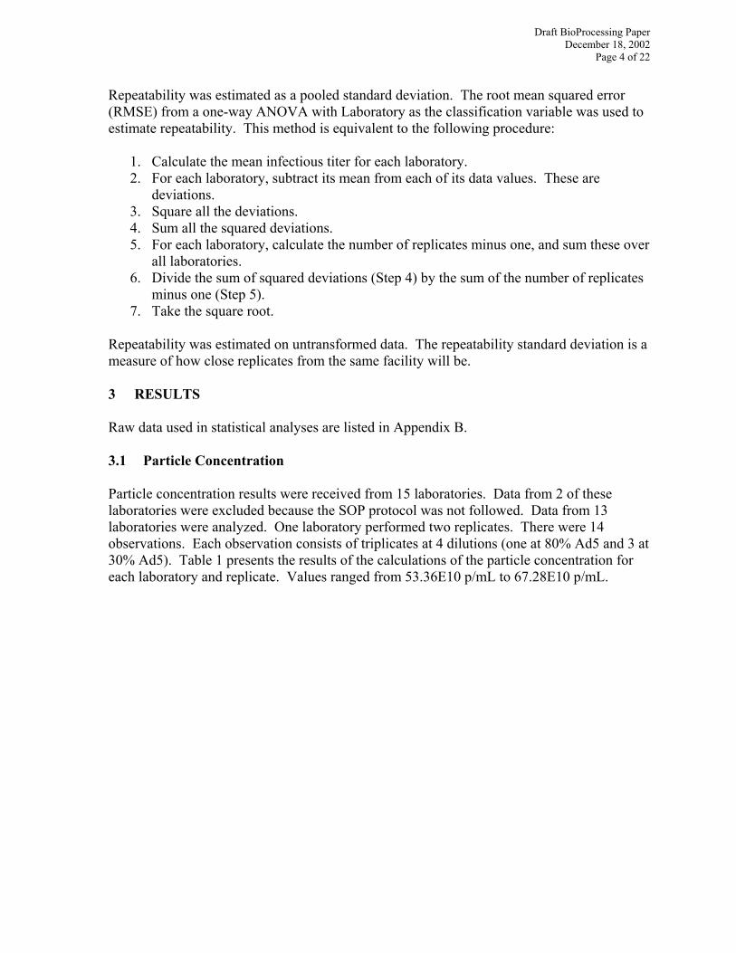
Repeatability was estimated as a pooled standard deviation. The root mean squared error (RMSE) from a one-way ANOVA with Laboratory as the classification variable was used to estimate repeatability. This method is equivalent to the following procedure:

1. Calculate the mean infectious titer for each laboratory. 2. For each laboratory, subtract its mean from each of its data values. These are

deviations. 3. Square all the deviations. 4. Sum all the squared deviations. 5. For each laboratory, calculate the number of replicates minus one, and sum these over

all laboratories. 6. Divide the sum of squared deviations (Step 4) by the sum of the number of replicates

minus one (Step 5). 7. Take the square root.

Repeatability was estimated on untransformed data. The repeatability standard deviation is a measure of how close replicates from the same facility will be. 3 RESULTS Raw data used in statistical analyses are listed in Appendix B. 3.1 Particle Concentration Particle concentration results were received from 15 laboratories. Data from 2 of these laboratories were excluded because the SOP protocol was not followed. Data from 13 laboratories were analyzed. One laboratory performed two replicates. There were 14 observations. Each observation consists of triplicates at 4 dilutions (one at 80% Ad5 and 3 at 30% Ad5). Table 1 presents the results of the calculations of the particle concentration for each laboratory and replicate. Values ranged from 53.36E10 p/mL to 67.28E10 p/mL.


Page 5 of 22

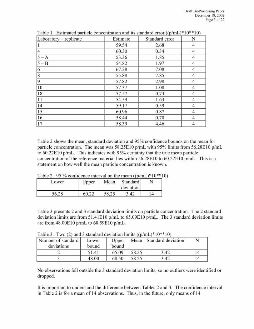
Table 1. Estimated particle concentration and its standard error ((p/mL)*10**10) Laboratory – replicate Estimate Standard error N 1 59.54 2.68 4 4 60.30 0.34 4 5 – A 53.36 1.85 4 5 – B 54.82 1.97 4 6 67.28 7.08 4 8 55.88 7.85 4 9 57.82 2.98 4 10 57.37 1.08 4 18 57.57 0.73 4 11 54.59 1.63 4 14 59.17 0.59 4 15 60.96 0.87 4 16 58.44 0.70 4 17 58.39 4.46 4 Table 2 shows the mean, standard deviation and 95% confidence bounds on the mean for particle concentration. The mean was 58.25E10 p/mL with 95% limits from 56.28E10 p/mL to 60.22E10 p/mL. This indicates with 95% certainty that the true mean particle concentration of the reference material lies within 56.28E10 to 60.22E10 p/mL. This is a statement on how well the mean particle concentration is known. Table 2. 95 % confidence interval on the mean ((p/mL)*10**10)

Lower Upper Mean Standard deviation

N

56.28 60.22 58.25 3.42 14 Table 3 presents 2 and 3 standard deviation limits on particle concentration. The 2 standard deviation limits are from 51.41E10 p/mL to 65.09E10 p/mL. The 3 standard deviation limits are from 48.00E10 p/mL to 68.59E10 p/mL. Table 3. Two (2) and 3 standard deviation limits ((p/mL)*10**10) Number of standard

deviations Lower bound

Upper bound

Mean Standard deviation N

2 51.41 65.09 58.25 3.42 14 3 48.00 68.50 58.25 3.42 14

No observations fell outside the 3 standard deviation limits, so no outliers were identified or dropped. It is important to understand the difference between Tables 2 and 3. The confidence interval in Table 2 is for a mean of 14 observations. Thus, in the future, only means of 14


Page 6 of 22

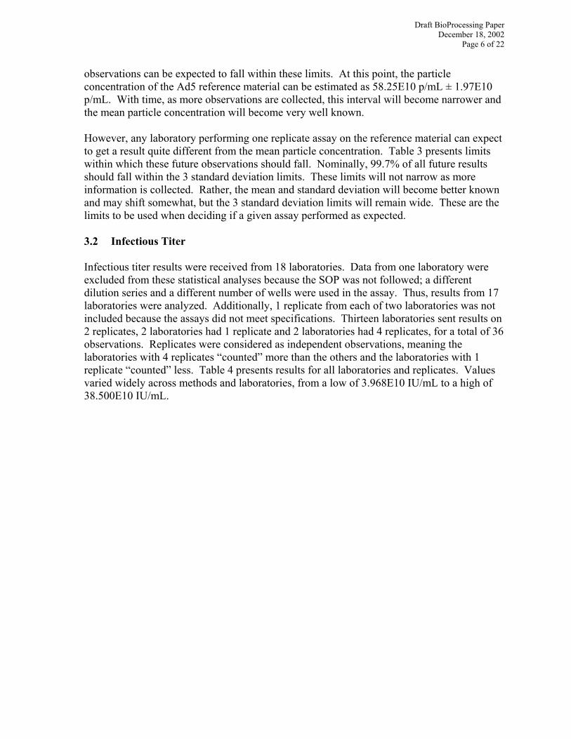
observations can be expected to fall within these limits. At this point, the particle concentration of the Ad5 reference material can be estimated as 58.25E10 p/mL ± 1.97E10 p/mL. With time, as more observations are collected, this interval will become narrower and the mean particle concentration will become very well known. However, any laboratory performing one replicate assay on the reference material can expect to get a result quite different from the mean particle concentration. Table 3 presents limits within which these future observations should fall. Nominally, 99.7% of all future results should fall within the 3 standard deviation limits. These limits will not narrow as more information is collected. Rather, the mean and standard deviation will become better known and may shift somewhat, but the 3 standard deviation limits will remain wide. These are the limits to be used when deciding if a given assay performed as expected. 3.2 Infectious Titer Infectious titer results were received from 18 laboratories. Data from one laboratory were excluded from these statistical analyses because the SOP was not followed; a different dilution series and a different number of wells were used in the assay. Thus, results from 17 laboratories were analyzed. Additionally, 1 replicate from each of two laboratories was not included because the assays did not meet specifications. Thirteen laboratories sent results on 2 replicates, 2 laboratories had 1 replicate and 2 laboratories had 4 replicates, for a total of 36 observations. Replicates were considered as independent observations, meaning the laboratories with 4 replicates “counted” more than the others and the laboratories with 1 replicate “counted” less. Table 4 presents results for all laboratories and replicates. Values varied widely across methods and laboratories, from a low of 3.968E10 IU/mL to a high of 38.500E10 IU/mL.


Page 7 of 22

Table 4. Estimated infectious titers ((IU/mL)*10**10) Laboratory - Replicate Average

Poisson Spearman-Kärber

untrimmed Spearman-Kärber

20% trim Spearman-Kärber

50% trim Maximum Likelihood

1 - A 7.811 10.960 9.351 7.584 8.867 1 - B 13.500 12.160 12.130 12.760 10.380 2 - A 36.340 11.630 38.500 36.080 35.720 2 - B 29.040 24.780 24.430 29.470 21.250 3 - A 8.761 8.763 7.750 8.271 7.522 3 - B 4.538 6.757 5.848 5.062 5.605 3 - C 5.834 5.136 4.659 4.778 4.444 3 - D 10.320 9.765 8.559 7.263 8.015 4 - B 7.772 6.610 5.552 3.968 5.434 5 - A 10.710 10.120 9.836 10.420 8.709 5 - B 10.460 8.391 7.722 6.378 7.018 6 - A 19.410 11.430 9.765 7.368 8.915 6 - B 9.383 7.695 6.470 4.381 6.210 7 - A 5.121 7.263 5.955 4.778 6.081 7 - B 4.894 5.933 5.305 4.778 5.024 8 - A 12.820 16.300 14.010 12.760 15.120 8 - B 10.560 9.836 9.907 10.120 8.279 9 - A 10.950 12.210 10.120 8.035 10.130 9 - B 13.600 11.360 10.800 9.019 9.586 10 - B 18.720 24.270 20.260 17.660 20.310 10 - C 21.080 24.620 21.010 21.010 20.400 11 - A 7.365 6.378 6.020 6.565 5.520 11 - B 6.201 7.476 6.684 5.682 6.274 11 - C 5.365 7.159 6.517 5.210 5.966 11 – D 9.045 9.979 9.217 8.513 8.520 12 – A 4.255 5.600 5.723 5.363 4.616 12 – B 6.265 5.441 5.580 6.020 4.561 13 – A 10.440 9.019 8.890 8.763 7.422 14 – A 7.727 8.637 8.006 8.035 7.418 14 – B 9.227 9.625 9.085 7.584 8.024 15 – A 9.002 9.907 8.778 8.890 8.485 15 - B 10.630 10.570 9.521 8.513 8.711 16 - A 7.666 10.350 9.385 10.120 8.801 16 - B 8.828 9.019 7.949 7.584 7.433 17 - A 15.590 15.390 15.390 14.320 12.090 17 - B 15.160 14.320 14.270 15.170 10.940

Table 5 presents the 95% confidence bounds and the 2 and 3 standard deviation confidence limits for all estimation methods. A comparison of this table with Table 4 shows that the values for laboratory # 2 are statistical outliers for the Spearman-Kärber 20% trim and maximum likelihood methods. The laboratory # 2 values for the other methods are outside the 2 standard deviation bounds (except the Spearman-Kärber untrimmed, replicate A). These two observations were subsequently dropped from the analysis.


Page 8 of 22

Table 5. Confidence bounds for infectious titers ((IU/mL)*10**10). All laboratories and all replicates Estimation method Arithmetic Geometric

mean 2 StD bounds 3 StD bounds 95% Bounds on

the mean

Mean StD Lower Upper Lower Upper Lower Upper N Average Poisson 11.23 6.75 9.84 3.64 26.65 2.21 43.85 8.32 11.65 36Spearman-Kärber 10.69 5.00 9.83 4.44 21.76 2.99 32.37 8.59 11.24 36Spearman-Kärber 20% trim 10.53 6.60 9.29 3.66 23.59 2.00 37.58 7.94 10.88 36Spearman-Kärber 50% trim 9.95 6.82 8.56 3.05 23.97 1.82 40.13 7.19 10.18 36Maximum likelihood 9.66 6.15 8.52 3.36 21.63 2.11 34.46 7.28 9.97 36 Table 6 presents confidence bounds for infectious titers without the outlier observations. All of the means and limits shifted lower. This is expected as an upper outlier was dropped. Also, the sample size dropped from 36 to 34 reflecting the loss of the two replicates from the one laboratory dropped. Table 6. Confidence bounds for infectious titers ((IU/mL)*10**10), Without Laboratory # 2 Estimation method Arithmetic Geometric


the mean

Mean StD Lower Upper Lower Upper Lower Upper N Average Poisson 9.97 4.24 9.18 4.01 20.97 2.66 31.70 7.94 10.60 34Spearman-Kärber 10.25 4.50 9.52 4.51 20.10 3.10 29.20 8.36 10.84 34Spearman-Kärber 20% trim 9.29 3.88 8.66 4.15 18.09 2.87 26.13 7.62 9.85 34Spearman-Kärber 50% trim 8.61 3.91 7.91 3.50 17.86 2.33 26.85 6.86 9.12 34Maximum likelihood 8.55 3.76 7.95 3.78 16.70 2.61 24.20 6.98 9.05 34 The ANOVA and regression results on passage number found no significant differences. Table 7 presents the p-values for these analyses and all are greater than 0.05. Table 7. P-values from ANOVAs Classification Variable Average

Poisson Spearman-

Kärber untrimmed

Spearman-Kärber 20%

trim

Spearman-Kärber 50%

trim

Maximum likelihood

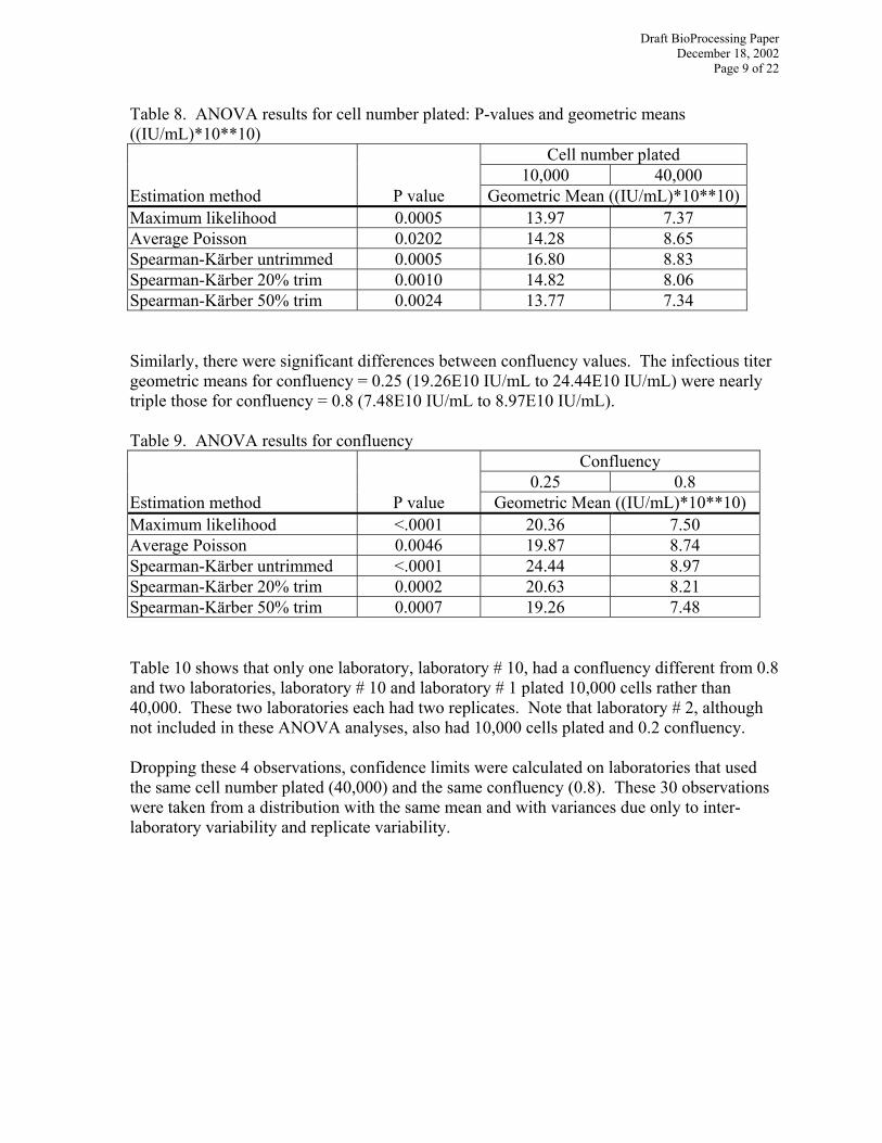
Passage Number Category 0.8636 0.4678 0.2811 0.1455 0.4836 Passage Number 0.6292 0.4350 0.2403 0.0783 0.3606 Significant differences were found between cell numbers plated. Table 8 shows that the p-values were less than 0.05 for all estimation methods. The infectious titer geometric means for 10,000 cells plated (13.77E10 IU/mL to 16.80E10 IU/mL) are nearly twice those for 40,000 cells plated (7.34E10 IU/mL to 8.83E10 IU/mL).


Page 9 of 22

Table 8. ANOVA results for cell number plated: P-values and geometric means ((IU/mL)*10**10)

Cell number plated 10,000 40,000 Estimation method P value Geometric Mean ((IU/mL)*10**10)Maximum likelihood 0.0005 13.97 7.37 Average Poisson 0.0202 14.28 8.65 Spearman-Kärber untrimmed 0.0005 16.80 8.83 Spearman-Kärber 20% trim 0.0010 14.82 8.06 Spearman-Kärber 50% trim 0.0024 13.77 7.34 Similarly, there were significant differences between confluency values. The infectious titer geometric means for confluency = 0.25 (19.26E10 IU/mL to 24.44E10 IU/mL) were nearly triple those for confluency = 0.8 (7.48E10 IU/mL to 8.97E10 IU/mL). Table 9. ANOVA results for confluency

Confluency 0.25 0.8 Estimation method P value Geometric Mean ((IU/mL)*10**10) Maximum likelihood <.0001 20.36 7.50 Average Poisson 0.0046 19.87 8.74 Spearman-Kärber untrimmed <.0001 24.44 8.97 Spearman-Kärber 20% trim 0.0002 20.63 8.21 Spearman-Kärber 50% trim 0.0007 19.26 7.48 Table 10 shows that only one laboratory, laboratory # 10, had a confluency different from 0.8 and two laboratories, laboratory # 10 and laboratory # 1 plated 10,000 cells rather than 40,000. These two laboratories each had two replicates. Note that laboratory # 2, although not included in these ANOVA analyses, also had 10,000 cells plated and 0.2 confluency. Dropping these 4 observations, confidence limits were calculated on laboratories that used the same cell number plated (40,000) and the same confluency (0.8). These 30 observations were taken from a distribution with the same mean and with variances due only to inter-laboratory variability and replicate variability.


Page 10 of 22

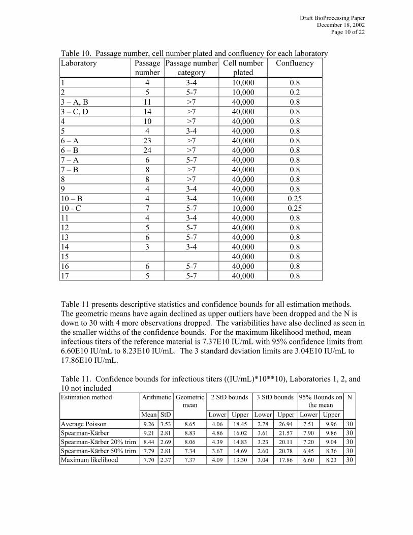
Table 10. Passage number, cell number plated and confluency for each laboratory Laboratory Passage

number Passage number

category Cell number

plated Confluency

1 4 3-4 10,000 0.8 2 5 5-7 10,000 0.2 3 – A, B 11 >7 40,000 0.8 3 – C, D 14 >7 40,000 0.8 4 10 >7 40,000 0.8 5 4 3-4 40,000 0.8 6 – A 23 >7 40,000 0.8 6 – B 24 >7 40,000 0.8 7 – A 6 5-7 40,000 0.8 7 – B 8 >7 40,000 0.8 8 8 >7 40,000 0.8 9 4 3-4 40,000 0.8 10 – B 4 3-4 10,000 0.25 10 - C 7 5-7 10,000 0.25 11 4 3-4 40,000 0.8 12 5 5-7 40,000 0.8 13 6 5-7 40,000 0.8 14 3 3-4 40,000 0.8 15 40,000 0.8 16 6 5-7 40,000 0.8 17 5 5-7 40,000 0.8 Table 11 presents descriptive statistics and confidence bounds for all estimation methods. The geometric means have again declined as upper outliers have been dropped and the N is down to 30 with 4 more observations dropped. The variabilities have also declined as seen in the smaller widths of the confidence bounds. For the maximum likelihood method, mean infectious titers of the reference material is 7.37E10 IU/mL with 95% confidence limits from 6.60E10 IU/mL to 8.23E10 IU/mL. The 3 standard deviation limits are 3.04E10 IU/mL to 17.86E10 IU/mL. Table 11. Confidence bounds for infectious titers ((IU/mL)*10**10), Laboratories 1, 2, and 10 not included Estimation method Arithmetic Geometric


the mean Mean StD Lower Upper Lower Upper Lower Upper

N

Average Poisson 9.26 3.53 8.65 4.06 18.45 2.78 26.94 7.51 9.96 30Spearman-Kärber 9.21 2.81 8.83 4.86 16.02 3.61 21.57 7.90 9.86 30Spearman-Kärber 20% trim 8.44 2.69 8.06 4.39 14.83 3.23 20.11 7.20 9.04 30Spearman-Kärber 50% trim 7.79 2.81 7.34 3.67 14.69 2.60 20.78 6.45 8.36 30Maximum likelihood 7.70 2.37 7.37 4.09 13.30 3.04 17.86 6.60 8.23 30


Page 11 of 22

Table 12 displays repeatability estimates for all estimation methods. Repeatability standard deviations vary from 1.47E10 IU/mL for 20% trimmed Spearman-Kärber to 2.46E10 IU/mL for the average Poisson. Repeatability measures how close replicates can be expected to be. Thus, smaller repeatability is better. For the maximum likelihood estimator, replicate observations should be within ± 3 x 1.60E10 IU/mL which equals ± 4.80E10 IU/mL. Table 12. Repeatability estimates ((IU/mL)*10**10) Estimation method Standard DeviationAverage Poisson 2.46 Spearman-Kärber 1.73 Spearman-Kärber 20% trim 1.47 Spearman-Kärber 50% trim 1.74 Maximum likelihood 1.60


Page 12 of 22

4 CONCLUSIONS The mean particle concentration was 5.825E11 p/mL with 95% limits from 5.628E11 p/mL to 6.022E11 p/mL. This means with 95% certainty the true mean particle concentration of the reference material lies within 5.628E11 p/mL to 6.022E10 p/mL. The WG decided to use the maximum likelihood results on data from laboratories that followed the stipulated protocol. The infectious titer was 7.37E10 IU/mL with 95% confidence limits from 6.60E10 IU/mL to 8.23E10 IU/mL. This means with 95% certainty the true mean infectious titer of the reference material lies within 6.60E10 IU/mL to 8.23E10 IU/mL. The WG also decided to keep 2 digits for particle concentration and one digit for infections titer. Thus, the particle concentration is 5.8 x 1011 particles/mL, with 95% certainty that the true particle concentration lies within the range of 5.6 x 1011 to 6.0 x 1011 particles/mL. The infectious titer on HEK 293 cells is 7 x 1010 NAS Infectious Units (NIU)/mL, with 95% certainty that the infectious titer on HEK 293 cells lies within the range of 7 x 1010 to 8 x 1010 NIU/mL.


Page 13 of 22

5 REFERENCES

1. Hutchins, B. (2002). Development of a Reference Material for Characterizing

Adenovirus Vectors. BioProcessing 1(1): 25-28. 2. Hutchins, B., Sajjadi, N., Seaver, S., Shepherd, A., Bauer, S.R., Simek, S., Carson,

K., and Aguilar-Cordova, E. (2000). Working Toward an Adenoviral Standard. Molecular Therapy 2(6): 532-534.

3. NIH Recombinant DNA Advisory Committee (January 2002) “NIH Report: Assessment of Adenoviral Vector Safety and Toxicity: Report of the National Institutes of Health Recombinant DNA Advisory Committee,” Human Gene Therapy 13 (1): 3-13.

4. Adenovirus Reference Material Standard Operating Procedure for Determination of Particle Concentration via Spectrophotometric Analysis, Version 4.0, Nov. 7, 2001.

5. Adenovirus Reference Material Standard Operating Procedure for Determination of Infectious Titer in 293 Cells in a 96-Well Format, Version 3.0, dated Nov. 7, 2001.


Page 14 of 22

APPENDIX A: ESTIMATION TECHNIQUES A-1 FORMULA FOR ESTIMATING PARTICLE CONCENTRATION Viral particle concentration was determined using the following formula: Concentration (particles/mL) = [A260nm corrected for blank] x [1.1E12 (particles/mL)] x [1/Dilution], where the dilutions were: 0.30 for the 30% Ad5 runs, and 0.80 for the 80% Ad5 runs, A260nm corrected for blank was the average of the triplicate readings corrected for blank, and the value of 1.1E12 particles/mL is from published data [1].


Page 15 of 22

A-2 FORMULAE FOR ESTIMATING INFECTOUS TITER UNITS Infectious titers were estimated with the following 5 methods: Average Poisson [2] (the default method in the Excel template), Spearman-Kärber [3], 20% trimmed Spearman-Kärber [4], 50% trimmed Spearman-Kärber [4], and maximum likelihood [5]. This section presents the formulae for the estimation. Section A-3 compares the methods and discusses pros and cons. Average Poisson The differential corrected infectious titer value was computed for each dilution for which the number of positive wells (out of 12) were greater than 2 and less than 10. This value was then averaged over the dilutions. The differential corrected infectious titer value was computed as follows:

(2 10)

(2 10)

ln 112

(0.32) (0.000238)

1d

d

dd

dF I

dp

p

pDdcitv

C T

dcitvdcitv < <

< <

− − =

=∑∑

Here, Dd is the dilution value for case d, pd is the number of positive wells at that dilution, CF is the confluency, and TI is the infection time. Spearman–Kärber The Spearman–Kärber method has four parts. The first part makes the data monotonic, the second part trims the edges, the third part performs the estimate of the 50% filled dilution, and the last part converts that result to the differential corrected infectious titer value. The non-trimmed case is calculated by setting the trimming parameter equal to zero. Monotonic transformation The monotonic transformation adjusts the data such that the positive well counts increase with a decrease in dilution. This is done by averaging the number of positive wells over neighboring dilutions. As a result the well counts will no longer be integers. Some experimentation was done to arrive at an algorithm that would successfully perform the monotonic transformation.


Page 16 of 22

a) The method mentioned in Hamilton et.al. was not efficient to implement as a computer algorithm. In this method, successive well counts are averaged if the second (less diluted) is smaller than the first (more diluted). This averaging is repeated until the sequence of well counts are non-decreasing. It was found that this procedure took over 10,000 iterations for one of the data sets. Most data sets converged in just a few iterations. A few took over a hundred iterations. (The convergence problems would be easily overcome if the adjustments were done manually.)

b) The method used converged in two iterations for all data sets. In this method dilution intervals are formed and averaged, and the average replaces the original values over the interval. A dilution interval extends from a beginning sample to the sample just before one that is larger than any sample in the interval. That larger sample is then the beginning sample in the next dilution interval.

Trimming Let yd be the monotonic transformed proportion of well occupancy (0 to 1.0) for a dilution index, d. Let α be the trim factor. (2α is the fraction trimmed.) Then the occupancies are adjusted as follows:

1 11 2

0 01 2

otherwise1 2

d

dd

d

y

yy

y

αααα

αα

− > − − = < −

− −

All proportions of well occupancies get changed by this algorithm. The proportions for the lowest, trimmed dilutions get set to zero. The proportions for the highest trimmed dilutions get set to one. The proportions in between get adjusted away from one-half. That is, some get adjusted higher and some get adjusted lower. The dilutions at the trimmed values may also get modified (See reference 3). Spearman-Kärber calculation The concentration at which 50% of the wells are positive is estimated to be

[ ]( )50 1 1exp 0.5 ln( ) ln( )d d d dd

LC D D y y+ +

= − − − −

∑

where the yd is the adjusted proportion at dilution Dd. This is related to concentration by


Page 17 of 22

50 ln 2C LC= Titer corrections To scale the LC50ln 2 to the differential corrected infectious titer value, the following equation was used:

50 ln 2(0.32) (0.000238)F I

LCdcitvC T

=

where Dd is the dilution value for case d, pd is the number of positive wells at that dilution, CF is the confluency, and TI is the infection time. Maximum Likelihood The samples are K replicates at each of N concentrations. The number of replicates with no entities is ki where 0 ≤ i < N-1. Each concentration has a dilution factor, di. The concentration at each dilution is represented by c/di where c is the unknown quantity to be estimated. The probability that no entities are detected in a sample is assumed to be Poisson and equal to

/ ic dip e−=

The dilution at which 50% of the samples would on average have zero entities is given by

50/

50

12

ln 2

c de

cd

−=

=

Then, the probability of obtaining the ki is given by a product of binomials as follows:

( )

( )

1

0

1/ /

0

1

1

ii

ii i i

NK kk

i ii i

N K kk c d c d

i i

KP p p

k

Ke e

k

−−

=

− −− −

=

= −

= −

∏

∏

The maximum likelihood estimate of the concentration, c, is found by differentiating this expression with respect to c, setting that expression equal to zero, and solving for c as follows:


Page 18 of 22

( )/1 1

/0 0

( )( ) 0

1

j

j

c dN Nj j

c dj jj j

k K k eP P P PA cc d d e

−− −

−= =

−∂= − + = = ∂ − ∑ ∑

where

( ) ( )( )

1

/0

1 01j

Nj

j c dj j

K kA c k

d e

−

=

− = − + = −

∑

A(c) must be zero since P is always positive and the product of A(c) and P is zero. Note that

( )1

0

(0)N

j

j j

Ak

Ad

−

=

= +∞

+∞ = −∑

In addition ( ) ( )

( )( )

/1

22 /00 0

1

j

j

c dNj

c dj j

K kA c e cc d e

−

=

−∂= − < < < +∞

∂ −∑

As A moves from positive infinity to a negative value as c goes from zero to infinity and the slope of A is negative throughout this region, A(c) only crosses zero once. Consequently there is a single solution for c. Also since A(c) is monotonic, it is relatively easy to iterate to a solution. To search for a solution, following steps are taken:

1 Pick an initial value for concentration, c, at the low end of the range.

2 Compute A(c). If A(c) is negative then divide c by two and repeat this step. If A(c) is positive, go to the next step.

3 Iterate updating c with

( )( )

A cc cA c

c

= −∂

∂ This seems to converge very well in a few iterations. The convergence is from the low side of the zero crossing.

The differential corrected infectious titer value is given by


Page 19 of 22

(0.32) (0.000238)F I

CdcitvC T

=

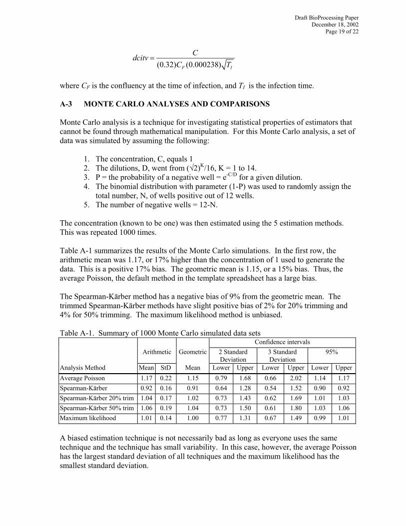
where CF is the confluency at the time of infection, and TI is the infection time. A-3 MONTE CARLO ANALYSES AND COMPARISONS Monte Carlo analysis is a technique for investigating statistical properties of estimators that cannot be found through mathematical manipulation. For this Monte Carlo analysis, a set of data was simulated by assuming the following:

1. The concentration, C, equals 1 2. The dilutions, D, went from (√2)K/16, K = 1 to 14. 3. P = the probability of a negative well = e-C/D for a given dilution. 4. The binomial distribution with parameter (1-P) was used to randomly assign the

total number, N, of wells positive out of 12 wells. 5. The number of negative wells = 12-N.

The concentration (known to be one) was then estimated using the 5 estimation methods. This was repeated 1000 times. Table A-1 summarizes the results of the Monte Carlo simulations. In the first row, the arithmetic mean was 1.17, or 17% higher than the concentration of 1 used to generate the data. This is a positive 17% bias. The geometric mean is 1.15, or a 15% bias. Thus, the average Poisson, the default method in the template spreadsheet has a large bias. The Spearman-Kärber method has a negative bias of 9% from the geometric mean. The trimmed Spearman-Kärber methods have slight positive bias of 2% for 20% trimming and 4% for 50% trimming. The maximum likelihood method is unbiased. Table A-1. Summary of 1000 Monte Carlo simulated data sets Confidence intervals Arithmetic Geometric 2 Standard

Deviation 3 Standard Deviation

95%

Analysis Method Mean StD Mean Lower Upper Lower Upper Lower Upper Average Poisson 1.17 0.22 1.15 0.79 1.68 0.66 2.02 1.14 1.17 Spearman-Kärber 0.92 0.16 0.91 0.64 1.28 0.54 1.52 0.90 0.92 Spearman-Kärber 20% trim 1.04 0.17 1.02 0.73 1.43 0.62 1.69 1.01 1.03 Spearman-Kärber 50% trim 1.06 0.19 1.04 0.73 1.50 0.61 1.80 1.03 1.06 Maximum likelihood 1.01 0.14 1.00 0.77 1.31 0.67 1.49 0.99 1.01

A biased estimation technique is not necessarily bad as long as everyone uses the same technique and the technique has small variability. In this case, however, the average Poisson has the largest standard deviation of all techniques and the maximum likelihood has the smallest standard deviation.


Page 20 of 22

Table A-2 presents the pros and cons for the estimation techniques. All techniques are biased except the maximum likelihood. The maximum likelihood also has the smallest variability. The average Poisson requires no iteration. Although the Spearman-Kärber method used in this report (the 0% trimmed Spearman-Kärber) required iteration, the traditional Spearman-Kärber does not. All Spearman-Kärber methods assume data have come from a symmetrical distribution so that the mean, which is actually estimated, can be set equal to the LC50, a median. See Finney [5] for further discussion of the Spearman-Kärber method. The maximum likelihood method has the most desirable properties among the estimation method investigated. Its biggest disadvantage is that it requires iterating. An Excel spreadsheet has been developed for evaluation. This spreadsheet requires a minimum amount of information to perform the iterating. Table A-2. Pros and Con of the estimation methods Analysis Method Biased Variability Iteration

RequiredAssumptions

Average Poisson Yes Largest No Restricted dilutions to 20% to 80% positive

Spearman-Kärber Yes 2nd smallest Yes 0% & 100% readings, symmetry, monotonicity

Spearman-Kärber 20% trim Yes middle Yes 0%, 100% readings, symmetry, monotonicity

Spearman-Kärber 50% trim Yes 2nd largest Yes 0%, 100% readings, symmetry, monotonicity

Maximum likelihood No Smallest Yes None


Page 21 of 22

A-4 APPENDIX REFERENCES 1. Maizel, JR., J., White, D., and Scharff, M. (1968). The Polypeptides of Adenovirus 1:

Evidence for Multiple Protein Components in the Virion and a Comparison of Types 2, 7A, and 12. Virology 36: 115-125.

2. Nyberg-Hoffman, C., Shabram, P., Li, Wei, Giroux, D. and Aguilar-Cordova, E. 1997. Sensitivity and reproducibility in adenoviral infectious titer determination. Nature Medicine 3(7): 808-811.

3. Finney, D.J. 1971. Statistical Method in Biological Assay. Second edition. P524-530. 4. Hamilton, M.A., Russo, R.C., and Thurston, R.V. 1977. Trimmed Spearman-Karber

method for estimating median lethal concentrations in toxicity bioassays. Environmental Science and Technology 11(7): 714–719.

5. Finney, D.J. 1971. Statistical Method in Biological Assay. Second edition. P520-522.


Page 22 of 22

APPENDIX B: DATA LISTING Table B-1. Listing of particle concentration data used in statistical analyses: A260nm blank corrected spectrophotometer readings Laboratory 80% Ad5 30% Ad5

# Replicate 1 Replicate 1 Replicate 2 Replicate 3 OD Reading OD Reading OD Reading OD Reading

1 2 3 1 2 3 1 2 3 1 2 3 1 0.406 0.401 0.405 0.165 0.168 0.168 0.166 0.166 0.166 0.164 0.166 0.1654 0.442 0.442 0.442 0.164 0.164 0.164 0.164 0.164 0.164 0.164 0.164 0.1645 – A 0.401 0.401 0.401 0.138 0.139 0.140 0.148 0.149 0.150 0.141 0.145 0.1465 – B 0.420 0.419 0.419 0.147 0.148 0.149 0.143 0.145 0.146 0.147 0.148 0.1486 0.444 0.446 0.446 0.210 0.210 0.211 0.188 0.183 0.183 0.174 0.172 0.1718 0.407 0.410 0.409 0.162 0.164 0.167 0.168 0.171 0.172 0.122 0.122 0.1229 0.415 0.412 0.414 0.170 0.170 0.169 0.157 0.153 0.153 0.151 0.152 0.15210 0.428 0.429 0.429 0.153 0.155 0.155 0.155 0.155 0.155 0.155 0.156 0.15618 0.420 0.420 0.420 0.159 0.158 0.158 0.158 0.158 0.159 0.154 0.154 0.15411 0.403 0.418 0.415 0.140 0.150 0.155 0.139 0.146 0.146 0.141 0.156 0.15014 0.429 0.430 0.430 0.160 0.159 0.159 0.162 0.163 0.164 0.161 0.163 0.16315 0.437 0.437 0.437 0.169 0.170 0.169 0.165 0.165 0.165 0.167 0.167 0.16716 0.432 0.433 0.433 0.158 0.158 0.158 0.159 0.159 0.159 0.159 0.159 0.15917 0.427 0.431 0.430 0.142 0.145 0.145 0.173 0.174 0.174 0.157 0.159 0.159


Page 23 of 22

Table B-2. Listing of infectious titer data used in statistical analyses: Number of positive wells.

Dilution (*107 ) Laboratory # - Replicate 5 10 20 28.3 40 56.6 80 113 160 226 620 453 640 12801 - A 12 11 12 8 4 5 4 3 2 2 1 2 1 0 1 - B 12 11 10 10 9 7 5 2 2 2 0 1 1 0 2 - A 12 11 12 9 7 4 3 4 0 1 0 0 2 1 2 - B 12 9 8 6 6 7 2 1 0 0 0 1 0 0 3 - A 12 12 8 7 7 4 6 1 1 0 2 1 0 0 3 - B 12 12 12 5 3 1 3 1 0 1 0 0 0 0 3 - C 12 7 7 6 5 6 2 1 1 0 1 0 0 0 3 - D 12 12 5 10 6 2 5 5 3 2 1 2 0 0 4 - B 12 12 7 4 2 4 2 4 3 1 0 0 1 0 5 - A 12 12 8 8 7 5 6 5 2 1 0 0 0 0 5 - B 12 12 9 4 8 3 2 2 4 3 0 0 0 0 6 - A 12 12 8 6 7 4 4 4 2 2 1 3 4 0 6 - B 12 11 5 7 4 3 2 2 3 4 2 2 1 0 7 - A 12 12 7 5 5 3 3 2 1 2 2 1 0 0 7 - B 12 12 7 6 3 4 2 0 2 0 0 0 0 0 8 - A 12 12 12 11 12 8 4 2 3 0 1 2 1 0 8 - B 12 11 10 7 6 6 6 4 1 1 0 1 0 0 9 - A 12 12 12 8 5 5 4 3 2 2 3 0 2 0 9 - B 12 12 10 7 8 5 4 3 1 4 3 0 0 0 10 - B 12 12 8 5 4 5 3 2 1 2 1 1 0 0 10 - C 12 10 8 7 6 4 3 2 1 1 1 2 1 0 11 - A 12 12 8 8 6 1 2 0 0 1 0 0 0 0 11 - B 12 12 9 5 5 3 2 3 2 2 0 0 0 0 11 - C 12 11 8 5 5 3 3 2 2 2 2 0 0 0 11 – D 12 12 11 7 5 5 6 2 2 1 1 0 0 0 12 – A 12 12 11 6 3 0 0 0 0 0 0 0 0 0 12 – B 12 12 9 7 4 0 0 0 0 0 0 0 0 0 13 – A 12 10 8 6 7 6 4 3 5 2 0 1 0 0 14 – A 12 11 9 9 7 3 3 1 2 2 1 1 0 0 14 – B 12 11 10 8 6 4 3 3 2 3 1 0 1 0 15 – A 12 12 8 9 7 4 4 4 1 1 2 1 0 0 15 - B 12 12 9 6 6 5 3 6 2 3 2 1 0 0 16 - A 12 12 7 10 10 3 4 4 1 1 1 0 1 0 16 - B 12 11 7 7 7 4 4 5 1 1 2 1 1 0 17 - A 12 11 10 9 8 7 6 4 4 3 3 2 1 0 17 - B 12 10 9 9 8 7 6 5 4 3 3 2 1 0

statistical analysis of adenovirus reference...

Documents