statisitcs tutorial v. s. reinhardt 10/17/01 page 1 space systems copyright 2005 victor s....

Statisitcs Tutorial V. S. Reinhardt 10/17/01

Space Systems

Copyright 2005 Victor S. Reinhardt--Rights to copy material is granted so long as a source reference is listed on each page, section, or graphic utilized.

Statistical Processes for Time and Frequency

A Tutorial

Victor S. Reinhardt10/17/01


Space Systems


Statistical Processes for Time and Frequency--Agenda

• Review of random variables

• Random processes

• Linear systems

• Random walk and flicker noise

• Oscillator noise


Space Systems


Review of Random Variables


Space Systems


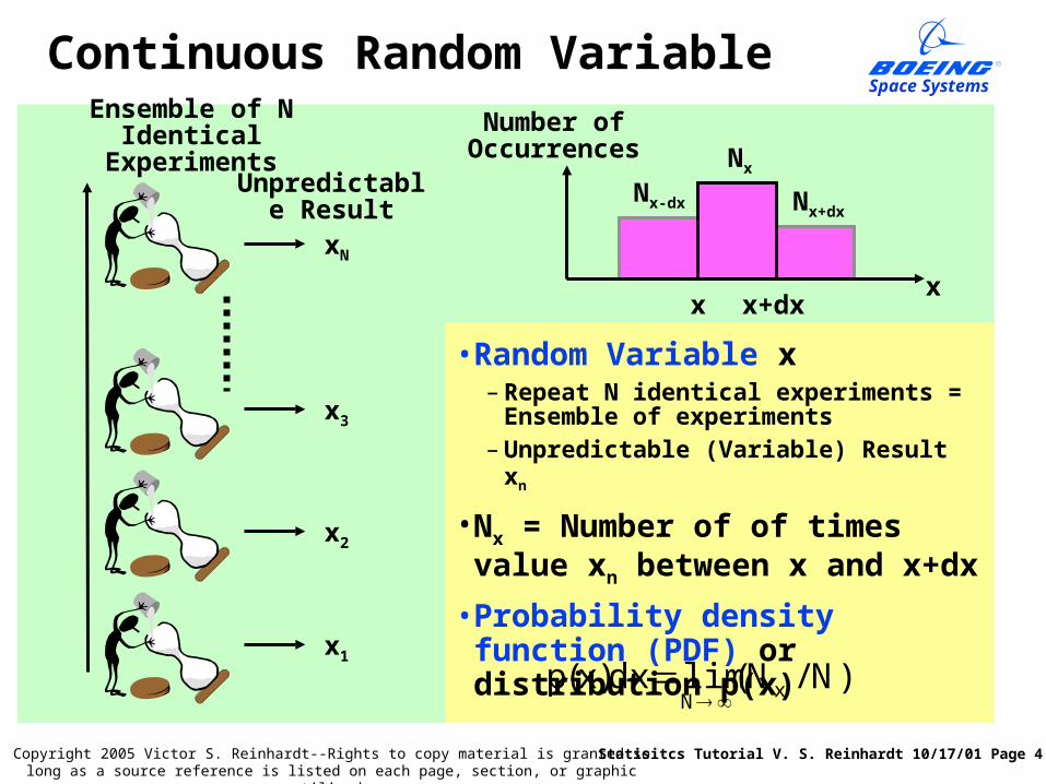
Continuous Random Variable

• Random Variable x– Repeat N identical experiments =

Ensemble of experiments

– Unpredictable (Variable) Result xn

• Nx = Number of of times value xn between x and x+dx

• Probability density function (PDF) or distribution p(x)

Ensemble of N Identical Experiments

Unpredictable Result

x1

x2

x3

xN

)N/N(limdx)x(p xN

x

Number ofOccurrences Nx

x x+dx

Nx+dxNx-dx


Space Systems


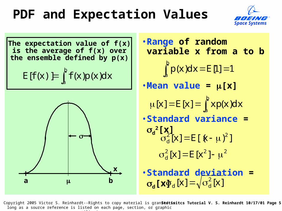
PDF and Expectation Values

• Range of random variable x from a to b

• Mean value = [x]

• Standard variance = d2[x]

• Standard deviation = d[x]

b

adx)x(xp]x[E]x[

b

a1]1[Edx)x(p

])x[(E]x[ 22d

222d ]x[E]x[

x

a b

The expectation value of f(x) is the average of f(x) over the ensemble

defined by p(x)

b

adx)x(p)x(f)]x(f[E

]x[]x[ 2dd


Space Systems


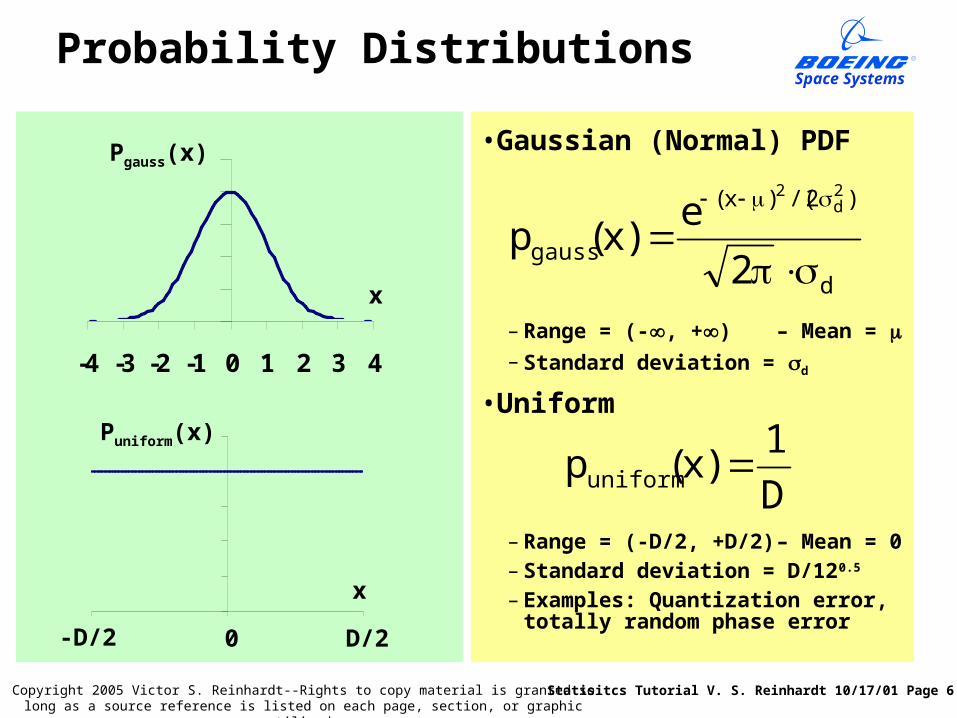
Probability Distributions

• Gaussian (Normal) PDF

– Range = (-, +) – Mean = – Standard deviation = d

• Uniform

– Range = (-D/2, +D/2) – Mean = 0

– Standard deviation = D/120.5

– Examples: Quantization error, totally random phase error

-4 -3 -2 -1 0 1 2 3 4

d

)2/()x(

gauss2

e)x(p

2d

2

Pgauss(x)

x

D

1)x(puniform

x

-D/2 D/20

Puniform(x)


Space Systems


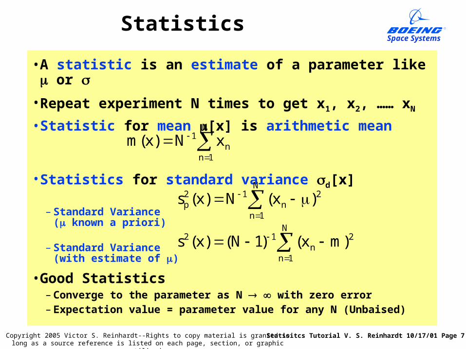
Statistics

• A statistic is an estimate of a parameter like or

• Repeat experiment N times to get x1, x2, …… xN

• Statistic for mean [x] is arithmetic mean

• Statistics for standard variance d[x]

– Standard Variance( known a priori)

– Standard Variance(with estimate of )

• Good Statistics– Converge to the parameter as N with zero error – Expectation value = parameter value for any N (Unbaised)

N

1nn

1 xN)x(m

N

1n

2n

12 )mx()1N()x(s

N

1n

2n

12p )x(N)x(s


Space Systems


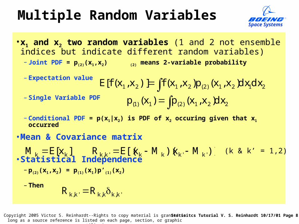
Multiple Random Variables

• x1 and x2 two random variables (1 and 2 not ensemble indices but indicate different random variables)– Joint PDF = p(2)(x1,x2) (2) means 2-variable probability

– Expectation value

– Single Variable PDF

– Conditional PDF = p(x1|x2) is PDF of x2 occuring given that x1 occurred

• Mean & Covariance matrix

• Statistical Independence– p(2)(x1,x2) = p(1)(x1)p’(1)(x2)

– Then

2121)2(2121 dxdx)x,x(p)x,x(f)]x,x(f[E

)]Mx)(Mx[(ER 'k'kkk'k,k ]x[EM kk

'k,kk,k'k,k RR

(k & k’ = 1,2)

221)2(1)1( dx)x,x(p)x(p


Space Systems


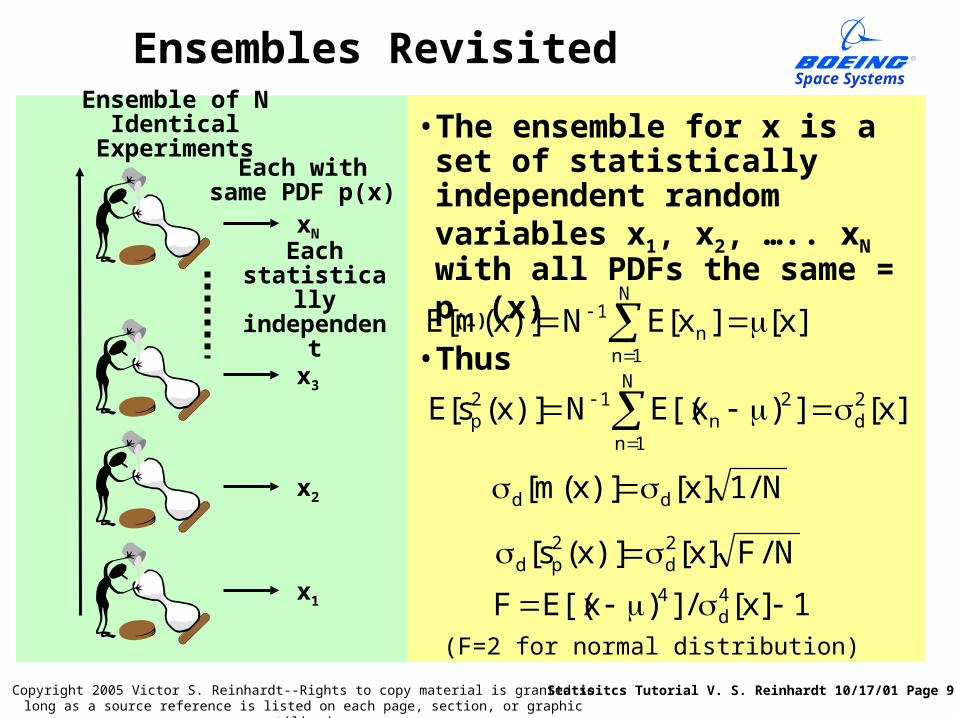
Ensembles Revisited

• The ensemble for x is a set of statistically independent random variables x1, x2, ….. xN

with all PDFs the same = p(1)(x)

• Thus

Ensemble of N Identical Experiments

x1

x2

x3

xN

Each with same PDF p(x)

Eachstatisticallyindependent ]x[]x[EN)]x(m[E

N

1nn

1

]x[])x[(EN)]x(s[E 2d

N

1n

2n

12p

N/1]x[)]x(m[ dd

N/F]x[)]x(s[ 2d

2pd

1]x[/])x[(EF 4d

4 (F=2 for normal distribution)


Space Systems


Random Processes


Space Systems


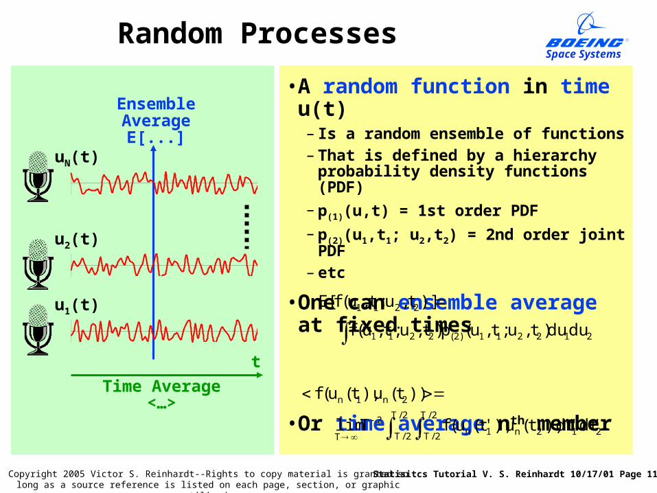
Random Processes

• A random function in time u(t)– Is a random ensemble of functions– That is defined by a hierarchy

probability density functions (PDF)

– p(1)(u,t) = 1st order PDF

– p(2)(u1,t1; u2,t2) = 2nd order joint PDF– etc

• One can ensemble average at fixed times

• Or time average nth member

Ensemble AverageE[...]

u1(t)

t

u2(t)

uN(t)

Time Average<…>

212211)2(2211

2211

dudu)t,u;t,u(p)t,u;t,u(f

)]t,u;t,u(f[E

2/T

2/T

2/T

2/T 212n1n2

T

2n1n

'dt'dt))'t(u),'t(u(fTlim

))t(u),t(u(f


Space Systems


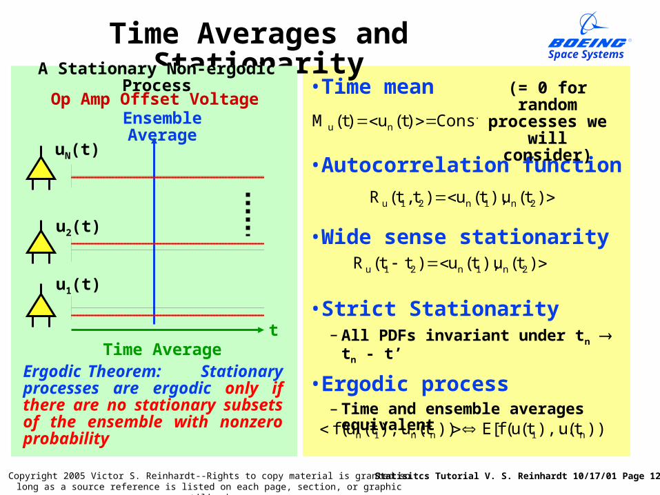
• Time mean

• Autocorrelation function

• Wide sense stationarity

• Strict Stationarity– All PDFs invariant under tn tn - t’

• Ergodic process– Time and ensemble averages

equivalent

Const )t(u)t(M nu

)t(u),t(u)t,t(R 2n1n21u

)t(u),t(u)tt(R 2n1n21u

Time Averages and Stationarity

(= 0 for random processes we will consider)

))]t(u),...t(u(f[E))t(u),...t(u(f n1nn1n

Ensemble Average

u1(t)

t

u2(t)

uN(t)

Time Average

A Stationary Non-ergodic Process

Ergodic_Theorem: Stationary processes are ergodic only if there are no stationary subsets of the ensemble with nonzero probability

Op Amp Offset Voltage


Space Systems


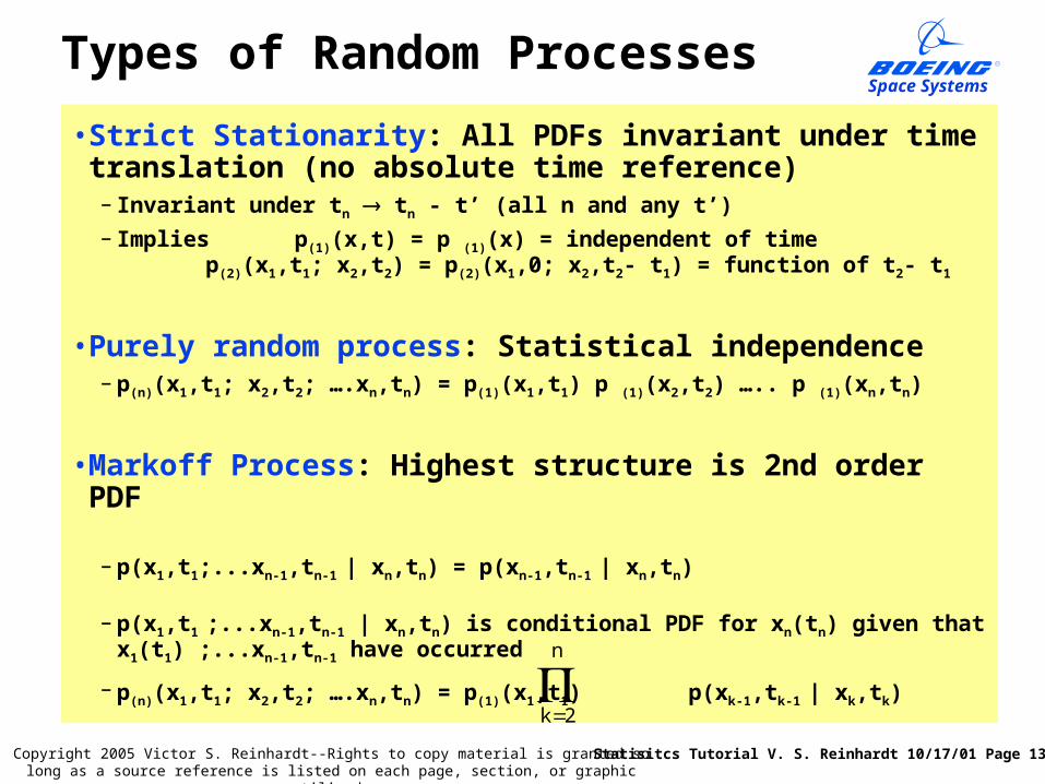
Types of Random Processes

• Strict Stationarity: All PDFs invariant under time translation (no absolute time reference)– Invariant under tn tn - t’ (all n and any t’)

– Implies p(1)(x,t) = p (1)(x) = independent of timep(2)(x1,t1; x2,t2) = p(2)(x1,0; x2,t2- t1) = function of t2- t1

• Purely random process: Statistical independence– p(n)(x1,t1; x2,t2; ….xn,tn) = p(1)(x1,t1) p (1)(x2,t2) ….. p (1)(xn,tn)

• Markoff Process: Highest structure is 2nd order PDF

– p(x1,t1;...xn-1,tn-1 | xn,tn) = p(xn-1,tn-1 | xn,tn)

– p(x1,t1 ;...xn-1,tn-1 | xn,tn) is conditional PDF for xn(tn) given thatx1(t1) ;...xn-1,tn-1 have occurred

– p(n)(x1,t1; x2,t2; ….xn,tn) = p(1)(x1,t1) p(xk-1,tk-1 | xk,tk)

n

2k


Space Systems


Linear Systems


Space Systems


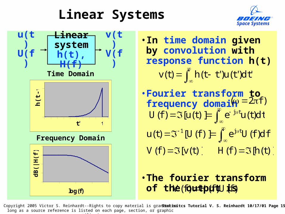
Linear Systems

• In time domain given by convolution with response function h(t)

• Fourier transform to frequency domain

• The fourier transform of the output is

u(t) Linear systemh(t), H(f)U(f)

v(t)

V(f)

'dt)'t(u)'tt(h)t(v

df)f(Ue)]f(U[)t(u tj1

)f2(

)]t(v[)f(V )]t(h[)f(H

)f(U)f(H)f(V log(f)

dB

(|H

(f)|

)

t'

h(t

-t')

t

Frequency Domain

Time Domain

dt)t(ue)]t(u[)f(U tj


Space Systems


U(f)V(f)R1

R2

C

-+

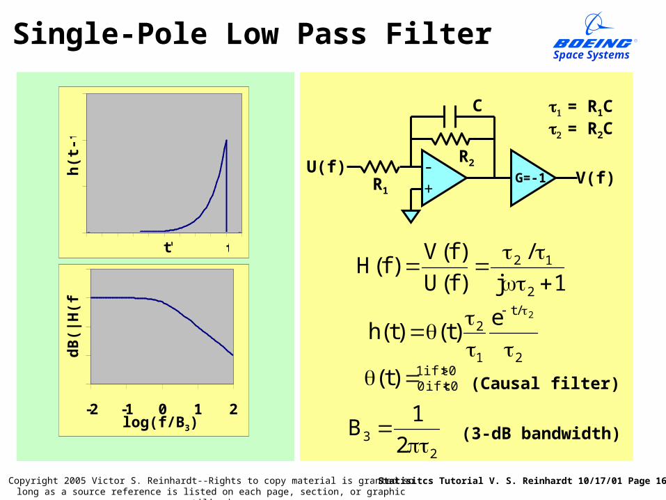
= R2C

G=-1

Single-Pole Low Pass Filter

1j

/

)f(U

)f(V)f(H

2

12

2

/t

1

22e

)t()t(h

0 tif 10 tif 0)t(

= R1C

23 2

1B

(3-dB bandwidth)

t'

h(t

-t')

t

-2 -1 0 1 2

dB

(|H

(f)|

)

log(f/B3)

(Causal filter)


Space Systems


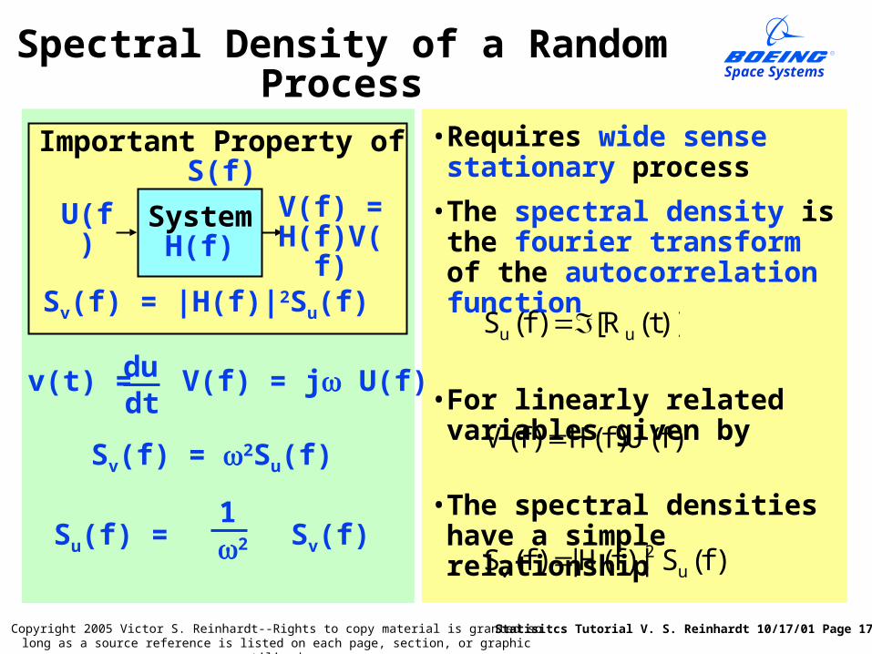
Spectral Density of a Random Process

• Requires wide sense stationary process

• The spectral density is the fourier transform of the autocorrelation function

• For linearly related variables given by

• The spectral densities have a simple relationship

Sv(f) = 2Su(f)

Su(f) = Sv(f) 12

v(t) = dudt

U(f) SystemH(f)

V(f) = H(f)V(f)

Sv(f) = |H(f)|2Su(f)

Important Property of S(f)

)]t(R[)f(S uu

)f(U)f(H)f(V

)f(S|)f(H|)f(S u2

v

V(f) = j U(f)


Space Systems


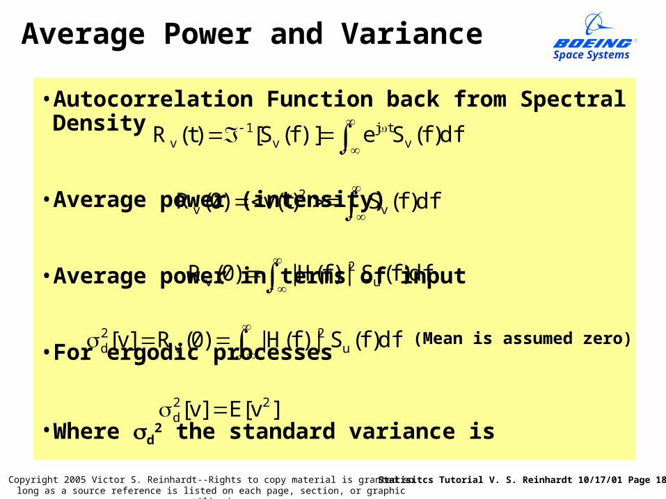
Average Power and Variance

• Autocorrelation Function back from Spectral Density

• Average power (intensity)

• Average power in terms of input

• For ergodic processes

• Where d2 the standard variance is

df)f(Se)]f(S[)t(R vtj

v1

v

df)f(S)t(v)0(R v

2v

df)f(S|)f(H|)0(R u

2v

df)f(S|)f(H|)0(R]v[ u

2v

2d

]v[E]v[ 22d

(Mean is assumed zero)


Space Systems


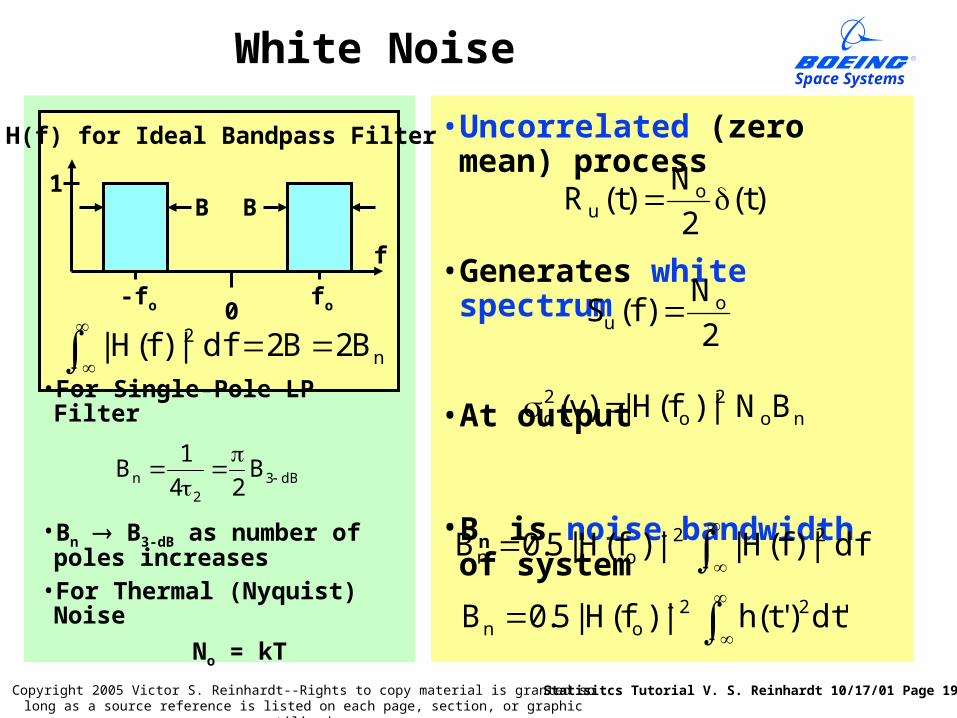
White Noise

• Uncorrelated (zero mean) process

• Generates white spectrum

• At output

• Bn is noise bandwidth of system

)t(2

N)t(R o

u

2

N)f(S o

u

df|)f(H||)f(H|5.0B 22on

'dt)'t(h|)f(H|5.0B 22on

no2

o2d BN|)f(H|)v(

H(f) for Ideal Bandpass Filter

n2 B2B2df|)f(H|

0

f

1BB

fo-fo

• For Single-Pole LP Filter

• Bn B3-dB as number of poles increases

• For Thermal (Nyquist) Noise

No = kT

dB32

n B24

1B


Space Systems


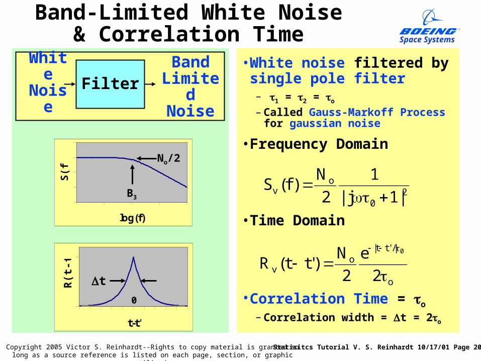
• White noise filtered by single pole filter– 1 = 2 = o

– Called Gauss-Markoff Process for gaussian noise

• Frequency Domain

• Time Domain

• Correlation Time = o

– Correlation width = t = 2o

WhiteNoise Filter

BandLimitedNoise

Band-Limited White Noise& Correlation Time

20

ov |1j|

1

2

N)f(S

o

/'|tt|o

v 2

e

2

N)'tt(R

0

log(f)

S(f

)

B3

No/2

t-t'

R(t

-t')

0

t


Space Systems


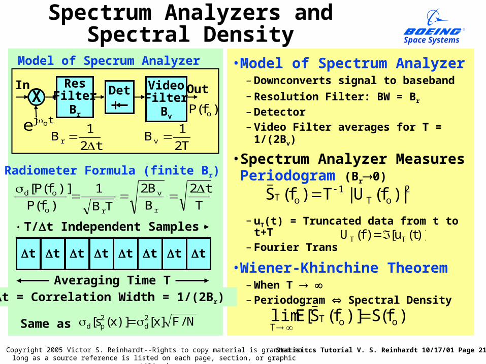
• Model of Spectrum Analyzer– Downconverts signal to baseband

– Resolution Filter: BW = Br – Detector

– Video Filter averages for T = 1/(2Bv)

• Spectrum Analyzer Measures Periodogram (Br0)

– uT(t) = Truncated data from t to t+T– Fourier Trans

• Wiener-Khinchine Theorem– When T – Periodogram Spectral Density

Spectrum Analyzers and Spectral Density

2oT

1oT

_

|)f(U|T)f(S

)]t(u[)f(U TT t t t t t

Averaging Time T

t

T/t Independent Samples

t t

t = Correlation Width = 1/(2Br)

)f(S)]f(S[Elim ooT

_

T

Radiometer Formula (finite Br)

T

t2

B

B2

TB

1

)f(P

)]f(P[

r

v

ro

od

Same as N/F]x[)]x(s[ 2d

2pd

Model of Specrum Analyzer

tj oe

ResFilter

Br

XIn Det Video

FilterBv

Out

t2

1Br

)f(P o

T2

1Bv


Space Systems


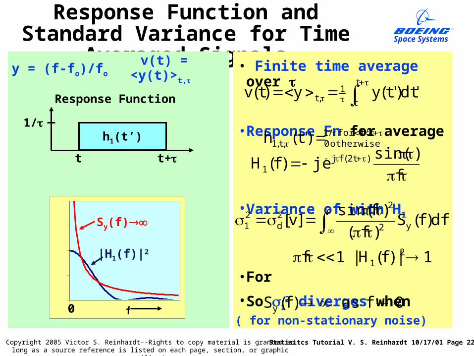
Response Function and Standard Variance for Time Averaged Signals

• Finite time average over

• Response Fn for average

• Variance of with H1

• For

• So 2 diverges when

tt'for t /1

otherwise 0,t,1 )'t(h

1|)f(H| 1f 21

0f as )f(S y f

|H1(f)|2

Sy(f)

0

t

t

1,t 'dt)'t(yy)t(v

1/h1(t’)

t+t

f

)sin(je)f(H )t2(fj

1

df)f(S)f(

)fsin(]v[ y2

22d

21

Response Function

( for non-stationary noise)

y = (f-fo)/fo v(t) = <y(t)>t,


Space Systems


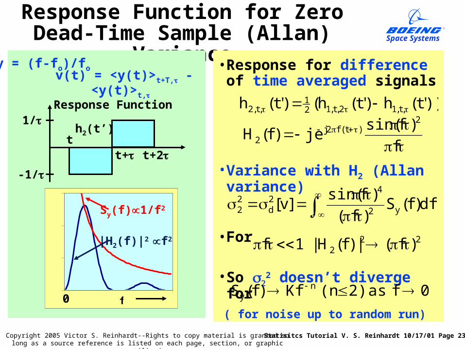
Response Function for Zero Dead-Time Sample (Allan) Variance

• Response for difference of time averaged signals

• Variance with H2 (Allan variance)

• For

• So 2 doesn’t diverge for

))'t(h)'t(h()'t(h ,t,12,t,121

,t,2 1/

f

)fsin(je)f(H

2)t(f2j

2

df)f(S)f(

)fsin(]v[ y2

42d

22

0f as 2)(n Kf)f(S ny

h2(t’)

-1/

t+t

t+2

222 )f(|)f(H| 1f

f

|H2(f)|2 f2

0

Sy(f)1/f2

Response Function

v(t) = <y(t)>t+T, - <y(t)>t,

( for noise up to random run)

y = (f-fo)/fo


Space Systems


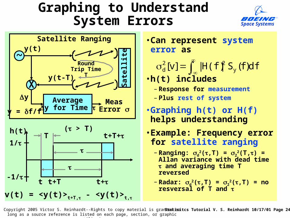
Graphing to Understand System Errors

• Can represent system error as

• h(t) includes– Response for measurement– Plus rest of system

• Graphing h(t) or H(f) helps understanding

• Example: Frequency error for satellite ranging– Ranging: d

2(,T) = 22(T,) = Allan

variance with dead time and averaging time T reversed

– Radar: d2(,T) = 2

2(,T) = no resversal of T and

df)f(S|H(f)|]v[ y

22d

~

Sat

elli

te

y(t)

X

Round Trip Time T

Averagey for Time

y(t-T)

Meas Error

Satellite Ranging

y = f/f

y

1/

-1/t

t+T t+

t+T+

v(t) = <y(t)>t+T, - <y(t)>t,

T( > T)h(t)


Space Systems


Random Walk and Flicker Noise


Space Systems


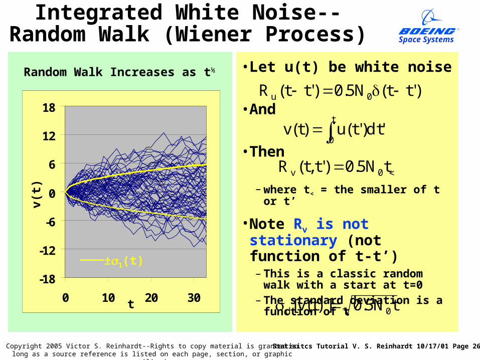
Integrated White Noise--Random Walk (Wiener Process)

• Let u(t) be white noise

• And

• Then

– where t< = the smaller of t or t’

• Note Rv is not stationary (not function of t-t’)– This is a classic random walk

with a start at t=0– The standard deviation is a

function of t

)'tt(N5.0)'tt(R 0u

t

0'dt)'t(u)t(v

tN5.0)'t,t(R 0v

tN5.0)]t(v[ 0d

Random Walk Increases as t½

-18

-12

-6

0

6

12

18

0 10 20 30

±1(t)

v(t)

t


Space Systems


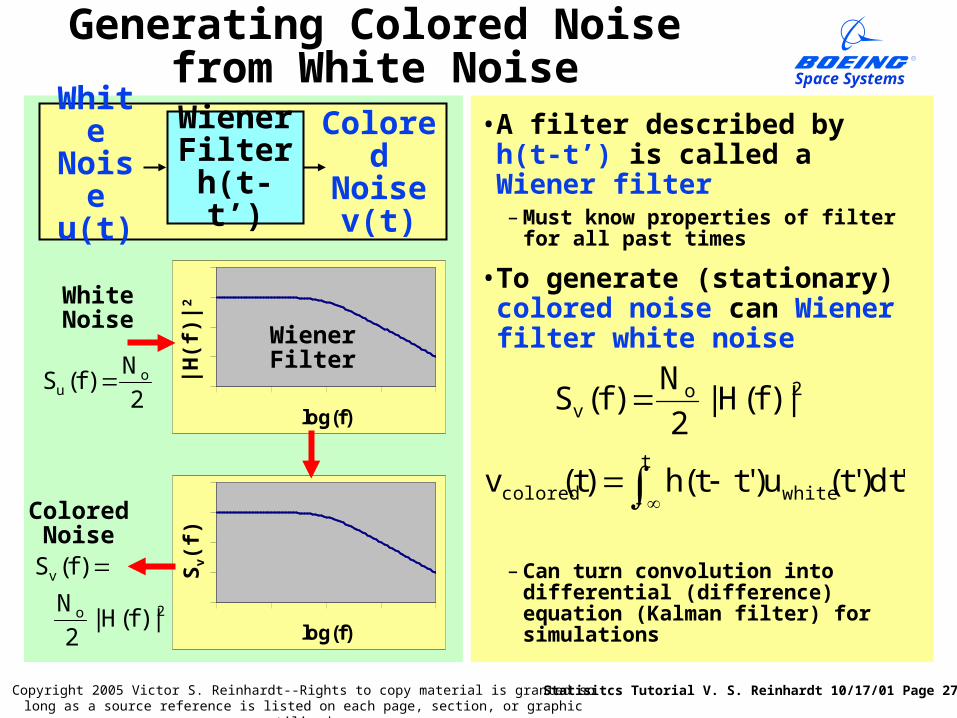
• A filter described by h(t-t’) is called a Wiener filter– Must know properties of filter for

all past times

• To generate (stationary) colored noise can Wiener filter white noise

– Can turn convolution into differential (difference) equation (Kalman filter) for simulations

WhiteNoiseu(t)

WienerFilterh(t-t’)

ColoredNoise

v(t)

Generating Colored Noise from White Noise

log(f)

|H(f

)|2

log(f)

Sv(

f)

2ov |)f(H|

2

N)f(S

t

whitecolored 'dt)'t(u)'tt(h)t(vColoredNoise

WienerFilter

2

N)f(S o

u

WhiteNoise

2o

v

|)f(H|2

N

)f(S


Space Systems


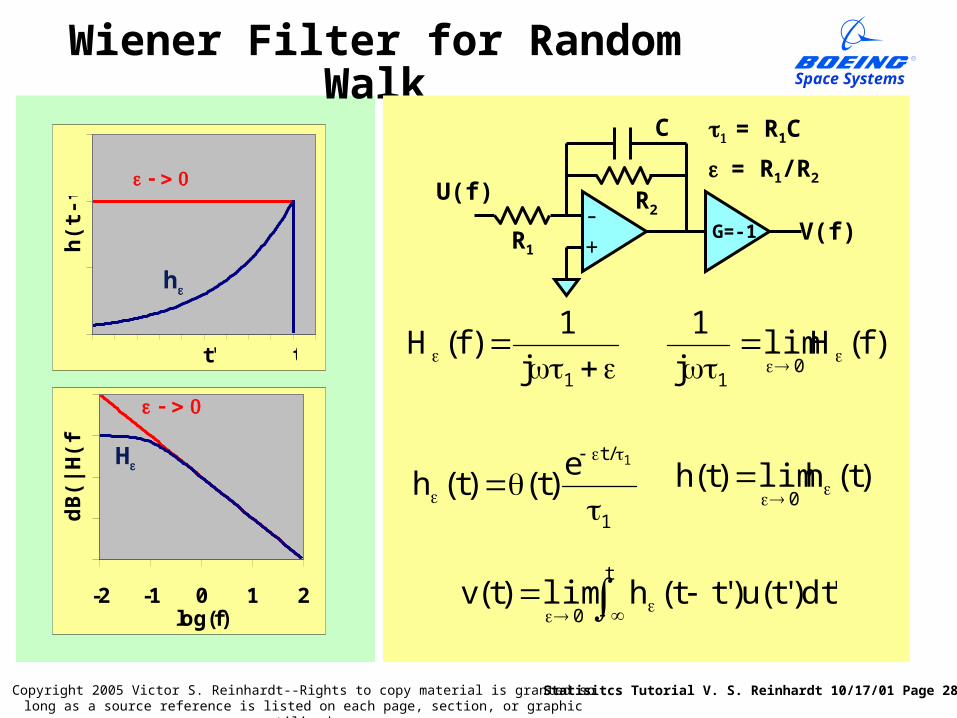
Wiener Filter for Random Walk

U(f)

R1

R2

C

-+

t

0'dt)'t(u)'tt(hlim)t(v

= R1C

= R1/R2

-2 -1 0 1 2log(f)

dB

(|H

(f)|

)

t'

h(t

-t')

t

H

h

V(f)G=-1

1j

1)f(H

1

/t 1e)t()t(h

)f(Hlimj

10

1

)t(hlim)t(h0


Space Systems


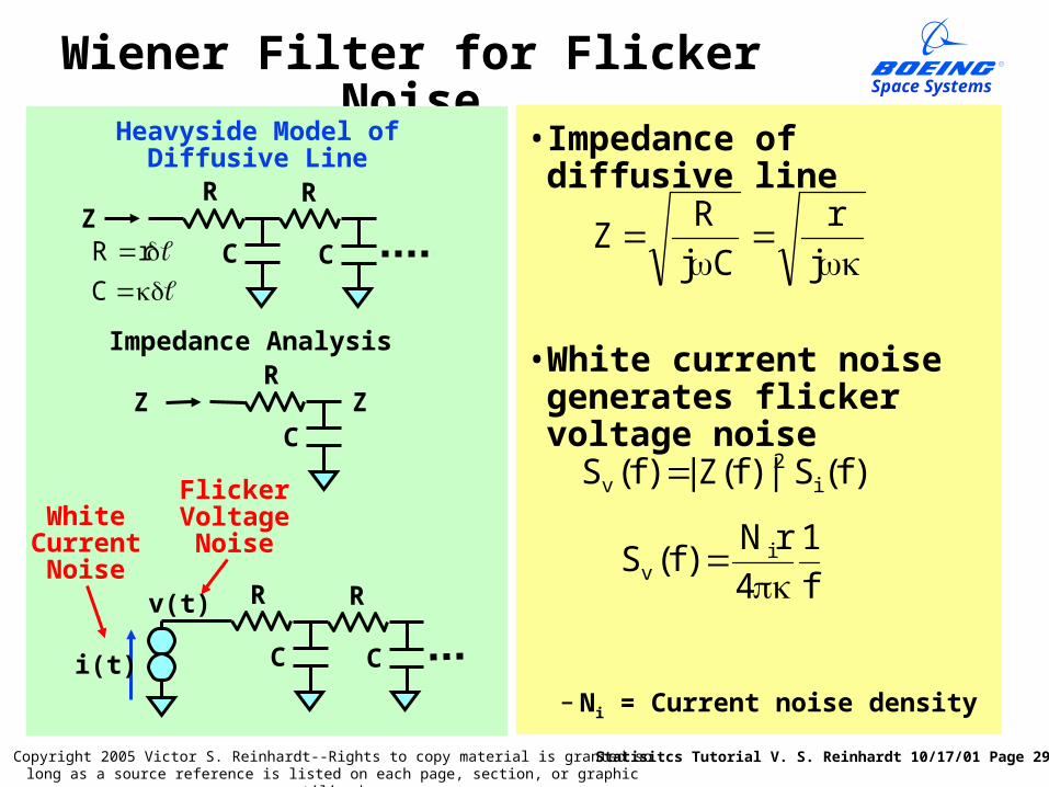
Wiener Filter for Flicker Noise

• Impedance of diffusive line

• White current noise generates flicker voltage noise

– Ni = Current noise density

R

C

R

CZ

Heavyside Model of Diffusive Line

C

rR

R

CZZ

Impedance Analysis

j

r

Cj

RZ

White Current Noise

Flicker Voltage Noise

R

C

R

C

v(t)

i(t)

)f(S|)f(Z|)f(S i2

v

f

1

4

rN)f(S i

v


Space Systems


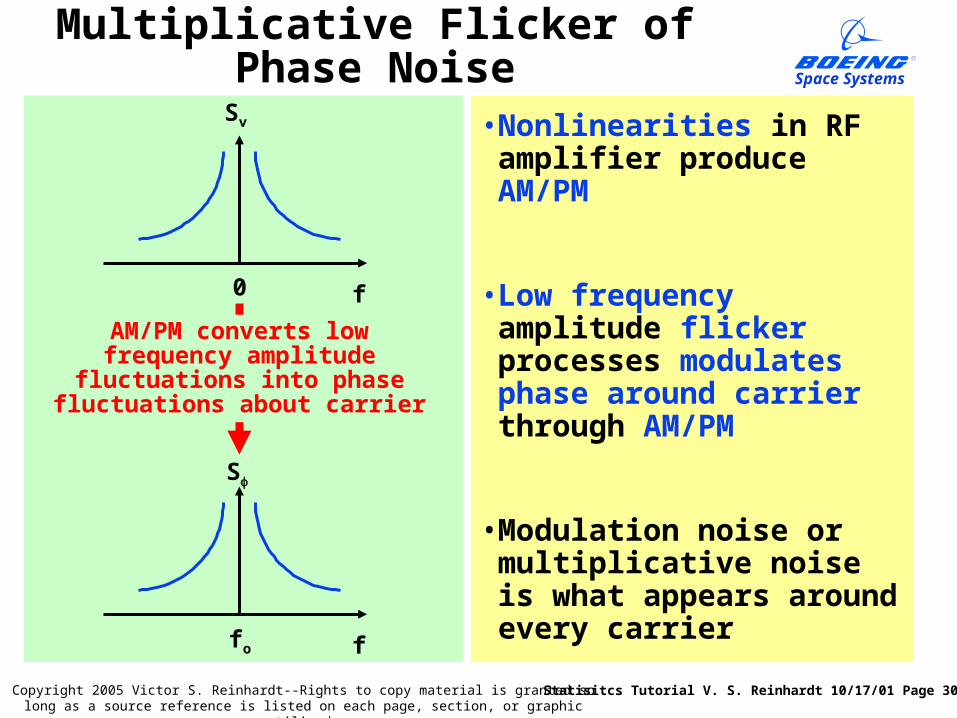
Multiplicative Flicker of Phase Noise

• Nonlinearities in RF amplifier produce AM/PM

• Low frequency amplitude flicker processes modulates phase around carrier through AM/PM

• Modulation noise or multiplicative noise is what appears around every carrier

Sv

f0

S

ffo

AM/PM converts low frequency amplitude fluctuations into

phase fluctuations about carrier


Space Systems


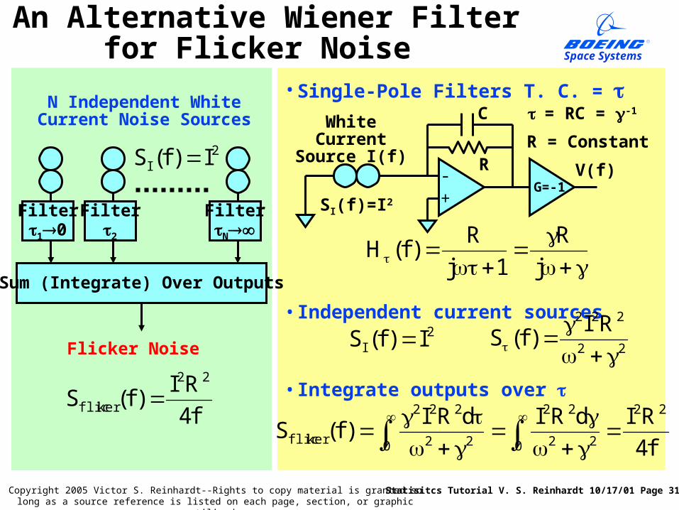
• Single-Pole Filters T. C. =

• Independent current sources

• Integrate outputs over

j

R

1j

R)f(H

22

222 RI)f(S

An Alternative Wiener Filter for Flicker Noise

f4

RIdRIdRI)f(S

22

0 22

22

0 22

222

kerflic

SI(f)=I2

V(f)R

C

-+

G=-1

= RC = -1

2I I)f(S

N Independent White Current Noise Sources

Filter10

Filter2

FilterN

Sum (Integrate) Over Outputs

Flicker Noise

f4

RI)f(S

22

kerflic

2I I)f(S

White Current Source I(f) R = Constant


Space Systems


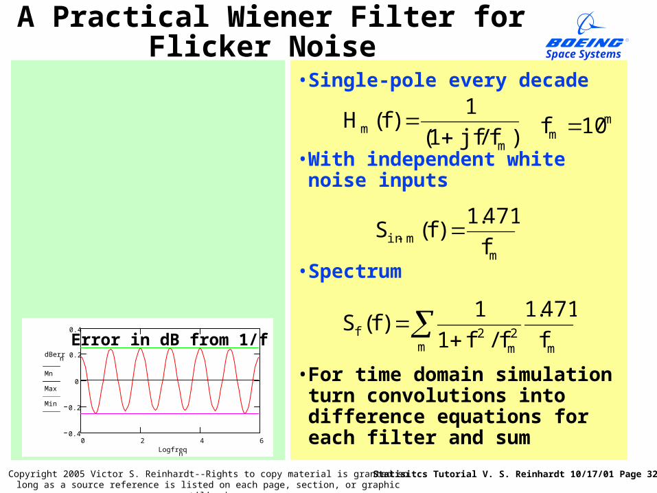
A Practical Wiener Filter for Flicker Noise

• Single-pole every decade

• With independent white noise inputs

• Spectrum

• For time domain simulation turn convolutions into difference equations for each filter and sum

)f/jf1(

1)f(H

mm

mm 10f

dBerrn

Mn

Max

Min

Logfreqn

0 2 4 60.4

0.2

0

0.2

0.4

mmin f

471.1)f(S

m m2m

2f f

471.1

f/f1

1)f(S

Error in dB from 1/f

0 1 2 3 4 5 660

50

40

30

20

10

0

Results for m = 0 to 8

Sf(f)

S (f)vm


Space Systems


Oscillator Noise


Space Systems


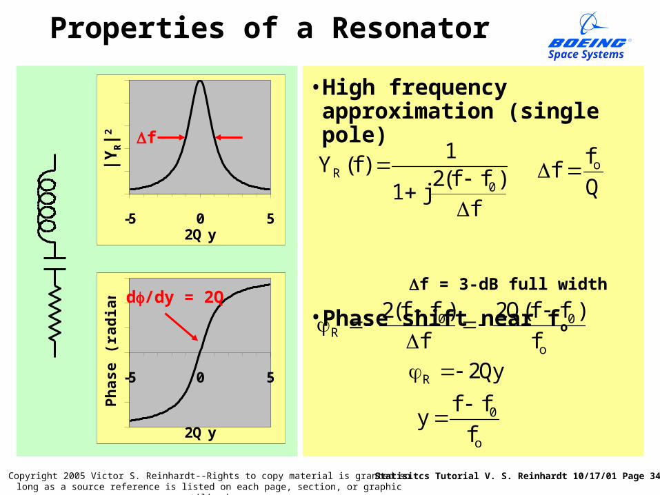
Properties of a Resonator

• High frequency approximation (single pole)

f = 3-dB full width

• Phase shift near fo

f)ff(2

j1

1)f(Y

0R

Q

ff o

o

00R f

)ff(Q2

f

)ff(2

Qy2R -5 0 5

2Q y

Ph

as

e (

rad

ian

s) d/dy = 2Q

o

0

f

ffy

-5 0 52Q y

f

|YR|2


Space Systems


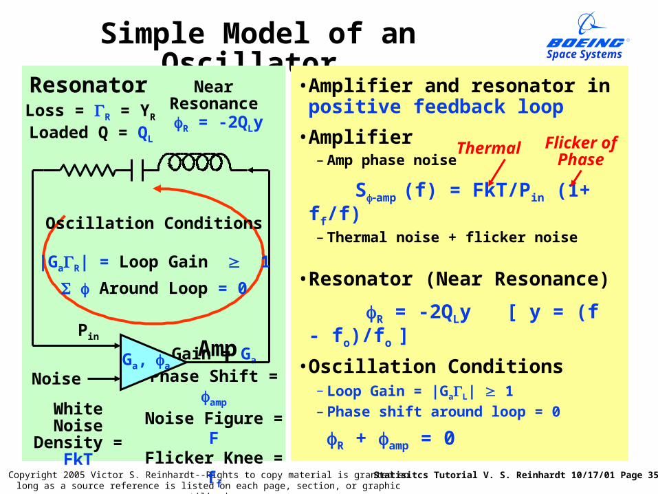
Simple Model of an Oscillator

• Amplifier and resonator in positive feedback loop

• Amplifier– Amp phase noise

Samp (f) = FkT/Pin (1+ ff/f)– Thermal noise + flicker noise

• Resonator (Near Resonance)

R = -2QLy [ y = (f - fo)/fo ]

• Oscillation Conditions– Loop Gain = |GaL| 1– Phase shift around loop = 0

R + amp = 0

Gain = Ga

Phase Shift = amp

Noise Figure = FFlicker Knee = ff

White Noise Density =

FkT

Resonator

Amp

Oscillation Conditions

|GaR| = Loop Gain 1

Around Loop = 0

Pin

NearResonance R = -2QLy

Loss = R = YR

Loaded Q = QL

NoiseGa,a

Thermal Flicker of Phase


Space Systems


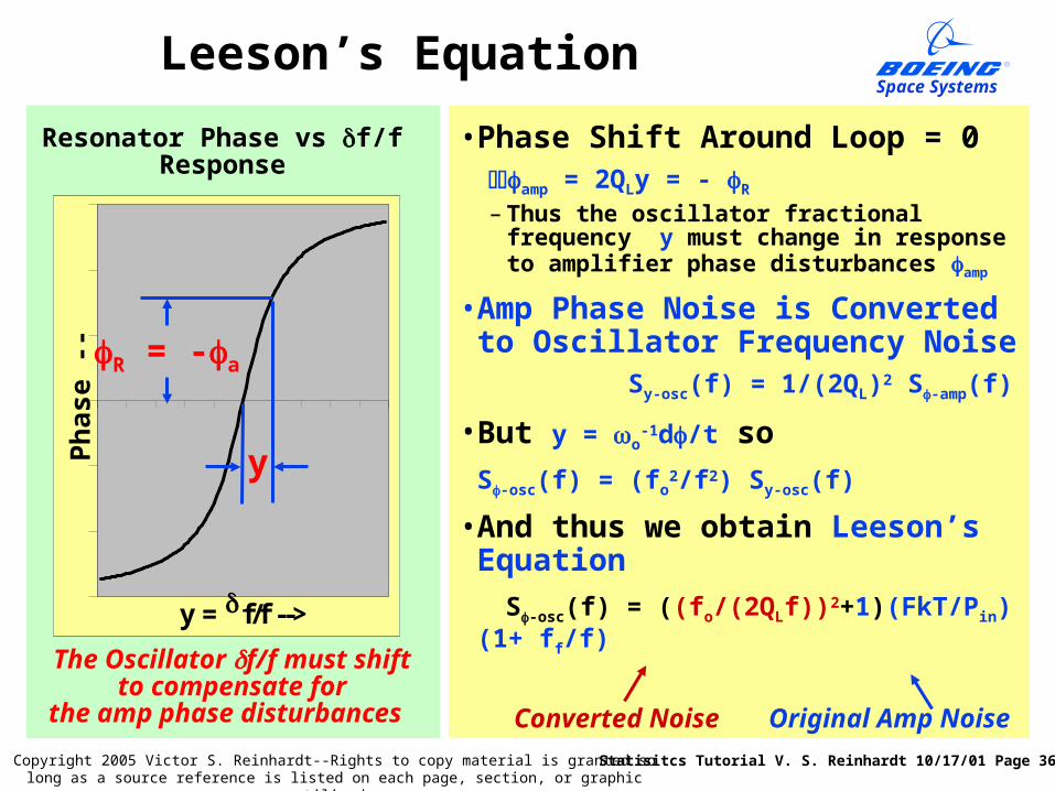
• Phase Shift Around Loop = 0amp = 2QLy = - R

– Thus the oscillator fractional frequency y must change in response to amplifier phase disturbances amp

• Amp Phase Noise is Converted to Oscillator Frequency Noise Sy-osc(f) = 1/(2QL)2 S-amp(f)

• But y = o-1d/t so

S-osc(f) = (fo2/f2) Sy-osc(f)

• And thus we obtain Leeson’s Equation

S-osc(f) = ((fo/(2QLf))2+1)(FkT/Pin)(1+ ff/f)

Leeson’s Equation

The Oscillator f/f must shift to compensate for

the amp phase disturbances Converted Noise Original Amp Noise

Resonator Phase vs f/fResponse

y = f/f -->

Ph

as

e -

->

y

R = -a


Space Systems


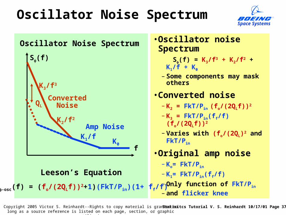
Oscillator Noise Spectrum

• Oscillator noise Spectrum S(f) = K3/f3 + K2/f2 + K1/f + K0

– Some components may mask others

• Converted noise– K2 = FkT/Pin (fo/(2QLf))2

– K3 = FkT/Pin(ff/f) (fo/(2QLf))2

– Varies with (fo/(2QL)2 and FkT/Pin

• Original amp noise– Ko= FkT/Pin

– K1= FkT/Pin(ff/f)

– Only function of FkT/Pin

– and flicker kneeS-osc(f) = (fo/(2QLf))2+1)(FkT/Pin)(1+ ff/f)

Oscillator Noise Spectrum

Leeson’s Equation

S(f)

f

K3/f3

K2/f2

K1/f K0

QL

Converted Noise

Amp Noise


Space Systems


References

• R. G. Brown, Introduction to Random Signal Analysis and Kalman Filtering, Wiley, 1983.

• D. Middleton, An Introduction to Statistical Communication Theory, McGraw-Hill, 1960.

• W. B, Davenport, Jr. and W. L. Root, An Introduction to the Theory of Random Signals and Noise, Mc-Graw-Hill, 1958.

• A. Van der Ziel, Noise Sources, Characterization, Measurement, Prentice-Hall, 1970.

• D. B. Sullivan, D. W. Allan, D. A. Howe, F. L. Walls, Eds, Characterization of Clocks and Oscillators, NIST Technical Note 1337, U. S. Govt. Printing office, 1990 (CODEN:NTNOEF).

• B. E. Blair, Ed, Time and Frequency Fundamentals, NBS Monograph 140, U. S. Govt. Printing office, 1974 (CODEN:NBSMA6).

• D. B. Leeson, “A Simple Model of Feedback Oscillator Noise Spectrum,” Proc, IEEE, v54, Feb., 1966, p329-335.

statisitcs tutorial v. s. reinhardt 10/17/01 page 1 space systems copyright 2005 victor s....

Documents