station automation and optimization of distribution ...€¦ · keywords: substation, automation,...
TRANSCRIPT

i
Energy Research and Development Division
FINAL PROJECT REPORT
Station Automation and Optimization of Distribution Circuit Operations
Gavin Newsom, Governor
March 2020 | CEC-500-2020-022

ii
PREPARED BY:
Primary Authors:
Ghazal Razeghi
Jennifer Lee
Scott Samuelsen
University of California, Irvine
Advanced Power and Energy Program
221 Engineering Lab Facility, Bldg. 323
Irvine, CA 92697-3550
(916) 824-7302 www.apep.uci.edu
Contract Number: EPC-15-086
PREPARED FOR:
California Energy Commission
David Chambers
Project Manager
Fernando Piña
Office Manager
ENERGY SYSTEMS RESEARCH OFFICE
Laurie ten Hope
Deputy Director
ENERGY RESEARCH AND DEVELOPMENT DIVISION
Drew Bohan
Executive Director
DISCLAIMER
This report was prepared as the result of work sponsored by the California Energy Commission. It does not necessarily
represent the views of the Energy Commission, its employees or the State of California. The Energy Commission, the
State of California, its employees, contractors and subcontractors make no warranty, express or implied, and assume
no legal liability for the information in this report; nor does any party represent that the uses of this information will
not infringe upon privately owned rights. This report has not been approved or disapproved by the California Energy
Commission nor has the California Energy Commission passed upon the accuracy or adequacy of the information in
this report.

i
ACKNOWLEDGEMENTS
The authors thank project partners OPAL-RT technologies and Southern California
Edison for their efforts and inputs to this project.

ii
PREFACE
The California Energy Commission’s (CEC) Energy Research and Development Division
supports energy research and development programs to spur innovation in energy
efficiency, renewable energy and advanced clean generation, energy-related
environmental protection, energy transmission and distribution and transportation.
In 2012, the Electric Program Investment Charge (EPIC) was established by the
California Public Utilities Commission to fund public investments in research to create
and advance new energy solutions, foster regional innovation and bring ideas from the
lab to the marketplace. The CEC and the state’s three largest investor-owned utilities—
Pacific Gas and Electric Company, San Diego Gas & Electric Company and Southern
California Edison Company—were selected to administer the EPIC funds and advance
novel technologies, tools, and strategies that provide benefits to their electric
ratepayers.
The CEC is committed to ensuring public participation in its research and development
programs that promote greater reliability, lower costs, and increase safety for the
California electric ratepayer and include:
• Providing societal benefits.
• Reducing greenhouse gas emission in the electricity sector at the lowest possible
cost.
• Supporting California’s loading order to meet energy needs first with energy
efficiency and demand response, next with renewable energy (distributed
generation and utility scale), and finally with clean, conventional electricity
supply.
• Supporting low-emission vehicles and transportation.
• Providing economic development.
• Using ratepayer funds efficiently.
Station Automation and Optimization of Distribution Circuit Operations is the final report
for the Station Automation and Optimization of Distribution Circuit Operations project
(Contract Number CEC-EPC-15-086) conducted by Advanced Power and Energy
Program, University of California Irvine. The information from this project contributes to
the Energy Research and Development Division’s EPIC Program.
For more information about the Energy Research and Development Division, please visit
the CEC’s research website (www.energy.ca.gov/research/) or contact the Energy
Commission at 916-327-1551.

iii
ABSTRACT
The University of California, Irvine’s Advanced Power and Energy Program used results,
insights, and capabilities from the Irvine Smart Grid Demonstration and Generic
Microgrid Controller projects to enhance substation control and distribution system
management. The project implemented a generic microgrid controller at a substation to
facilitate (1) maximizing the penetration of distributed energy resources, (2) assessing
the viability of a retail/distribution electricity market, (3) developing strategies for a
better distribution system management and use of smart grid technologies, and (4)
simulating and assessing deployed fuel cells at the substation.
The research team used generic microgrid controller specifications to develop a
controller for simulation of two 12 kilovolt distribution circuits at a distribution
substation. The circuits and the controller were simulated using an OPAL-RT simulation
platform. The results of the simulations were then used to determine the benefits of the
distributed energy resources dispatched by the controller simulated at the substation.
Results of the simulation show that using a controller at the substation facilitates an
increase in the renewable penetration and associated reduction in greenhouse gas
emissions. Larger batteries on the utility side result in higher renewable penetration at a
lower cost compared to residential storage on the customer side. Circuit battery and
demand response can alleviate the “duck curve,” fuel cell deployment at the substation
increases reliability significantly, and retail customer participation in a distribution
electricity market can reduce customer energy bills.
Keywords: Substation, automation, distribution system management, distribution
system control, distributed energy resources, controller
Please use the following citation for this report:
Razeghi, Ghazal, Jennifer Lee, Scott Samuelsen. Advanced Power and Energy Program.
2020. Station Automation and Optimization of Distribution Circuit Operations.
California Energy Commission. Publication Number: CEC-500-2020-022.

iv
TABLE OF CONTENTS
Page
ACKNOWLEDGEMENTS ............................................................................................... i
PREFACE .................................................................................................................. ii
ABSTRACT ............................................................................................................... iii
EXECUTIVE SUMMARY .............................................................................................. 1
Introduction ........................................................................................................... 1
Project Purpose ...................................................................................................... 1
Project Approach .................................................................................................... 2
Project Conclusions ................................................................................................ 3
Technology/Knowledge Transfer ............................................................................. 4
Conferences ........................................................................................................ 5
Publications ......................................................................................................... 5
Benefits to California .............................................................................................. 5
Recommendations .................................................................................................. 6
CHAPTER 1: Introduction .......................................................................................... 7
Project Tasks ......................................................................................................... 8
Task 1: General Project Tasks .............................................................................. 8
Task 2: Base Model Development ......................................................................... 8
Task 3: Scenario Development ............................................................................. 8
Task 4: Controller Development ........................................................................... 9
Task 5: Retail/Distribution Market ......................................................................... 9
Task 6: Evaluation of Project Benefits ................................................................. 10
Task 7: Technology/Knowledge Transfer Activities ............................................... 10
Irvine Smart Grid Demonstration Project ................................................................ 10
Generic Microgrid Controller .................................................................................. 13
CHAPTER 2: Task 2: Base Model Development ......................................................... 16
OPAL-RT Setup .................................................................................................... 16
System Model and Load Flow ................................................................................ 17
Load Flow Analysis ............................................................................................ 20
CHAPTER 3: Task 3: Scenario Development .............................................................. 23

v
Methodology ........................................................................................................ 23
Scenarios ............................................................................................................. 25
Scenario 1: High Renewable Penetration ............................................................. 25
Scenario 2: Energy Storage ................................................................................ 26
Scenario 4: Circuit-Independent ......................................................................... 27
CHAPTER 4: Task 4: Controller Development ............................................................ 28
Device (Local) Controllers ..................................................................................... 29
Residential Energy Storage Unit ......................................................................... 29
Community Energy Storage ................................................................................ 33
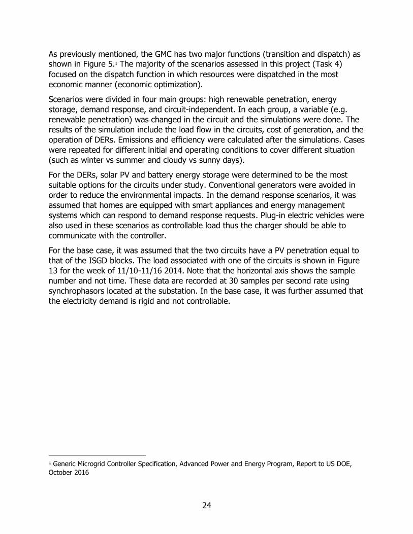
Circuit Battery ................................................................................................... 38
Fuel Cell............................................................................................................ 39
Demand Response ............................................................................................. 42
Controller Logic .................................................................................................... 45
Business as Usual .............................................................................................. 47
Circuit-Independent ........................................................................................... 50
CHAPTER 5: Simulation Results and Discussion ......................................................... 51
Scenario 1 ........................................................................................................... 51
Scenario 2 ........................................................................................................... 54
Residential Energy Storage Units ........................................................................ 56
Community Energy Storage ................................................................................ 61
Simulations with Various Photovoltaic Profiles ..................................................... 67
Renewable Penetration ...................................................................................... 71
Circuit Battery ................................................................................................... 72
Scenario 3 ........................................................................................................... 74
Scenario 4 ........................................................................................................... 76
CHAPTER 6: Task 5: Retail/Distribution Market ......................................................... 83
Electricity Markets and Market Participation for Distributed Energy Resources .......... 83
DER Wholesale Market Participation Benefits (Existing Opportunities) ...................... 84
Possible Future Opportunities: Distribution/Retail Markets....................................... 90
Participation of Retail Customers (Retail Market) ................................................. 95
Distribution Market Challenges ........................................................................... 98
Suggested Changes ............................................................................................ 100

vi
Costs .............................................................................................................. 101
Benefits .......................................................................................................... 101
CHAPTER 7: Benefits of the Project ........................................................................ 103
Reduced Emissions ............................................................................................. 103
Improved Reliability ............................................................................................ 107
Lower Costs ....................................................................................................... 109
Other Benefits .................................................................................................... 110
Reduced Fossil Fuel Usage ............................................................................... 110
Reduced Energy Demand ................................................................................. 110
Increased Safety ............................................................................................. 110
Energy Security ............................................................................................... 110
Enhanced Resiliency ........................................................................................ 110
Reduced RPS Procurement ............................................................................... 111
Avoided Transmission Upgrade Costs ................................................................ 111
CHAPTER 8: Conclusions ....................................................................................... 112
Major Findings ................................................................................................... 112
Recommendations and Future Work .................................................................... 113
LIST OF ACRONYMS .............................................................................................. 115
REFERENCES ........................................................................................................ 119
APPENDIX A: Test Case Templates ........................................................................ A-1
APPENDIX B: Interconnection/Market Overview ...................................................... B-1

vii
LIST OF FIGURES
Page
Figure 1. ISGD Project ............................................................................................. 11
Figure 2. Load sample of a home in the ZNE block .................................................... 11
Figure 3. PV and RESU sample data for a home in the ZNE block ............................... 12
Figure 4. EV data for June 2014 ............................................................................... 12
Figure 5. GMC Levels of Control ............................................................................... 15
Figure 6. GMC Modular Architecture ......................................................................... 15
Figure 7. OPAL-RT .................................................................................................. 17
Figure 8. OPAL-RT setup ......................................................................................... 17
Figure 9. Circuit model ............................................................................................ 18
Figure 10. Home Model with PV and Battery ............................................................. 19
Figure 11. Dynamic Load Model ............................................................................... 20
Figure 12. Circuit with Voltage Unbalance ................................................................. 21
Figure 13. Real power (MW)- Circuit A ..................................................................... 25
Figure 14. Controller schematic and levels of control ................................................. 29
Figure 15. RESU Component .................................................................................... 30
Figure 16. RESU Component Mask, Power Tab .......................................................... 30
Figure 17. RESU Component Mask, Control Tab ........................................................ 31
Figure 18. RESU Simulation Results, PV Capture Mode .............................................. 32
Figure 19. RESU Simulation Results, Time-Based Load Shifting Mode ......................... 33
Figure 20. CES Component ...................................................................................... 34
Figure 21. CES Component Mask, Power Tab ............................................................ 34
Figure 22. CES Component Mask, Permanent Load Shifting Mode Tab ........................ 35
Figure 23. CES Component Mask, Load Limiting Mode ............................................... 36
Figure 24. CES Simulation Results, Permanent Load Shifting Mode ............................. 37
Figure 25. CES Simulation Results, Load Limiting Mode ............................................. 38
Figure 26. Circuit Battery Component ....................................................................... 39
Figure 27. Fuel Cell Component ............................................................................... 39

viii
Figure 28. Fuel Cell Component Mask, Power Tab ..................................................... 40
Figure 29. Fuel Cell Component Mask, Base Load Mode ............................................. 40
Figure 30. Fuel Cell Component Mask, Load Limiting Mode ........................................ 41
Figure 31. Fuel Cell Simulation at the Substation – Base Load Mode Result ................. 42
Figure 32. Fuel Cell Simulation at the Substation - Load Follow Mode Result ............... 42
Figure 33. Demand Response – Result ..................................................................... 43
Figure 34. EVSE Mask Model .................................................................................... 44
Figure 35. EVSE Demand Response Simulation – Result ............................................ 45
Figure 36. Controller Logic ....................................................................................... 46
Figure 37. Economic Dispatch .................................................................................. 47
Figure 38. Residential and Commercial Areas in the Two Circuits ............................... 51
Figure 39. Building Rooftop Footprint (One Section) .................................................. 52
Figure 40. Overvoltage at a Node with Max PV Based on Footprint ............................. 53
Figure 41. Voltage at a Node with a New Adjusted PV Penetration ............................. 53
Figure 42. Block Load and PV Profile – 5/15/2014 ..................................................... 55
Figure 43. Average EV Charging Schedule per Home ................................................. 55
Figure 44. Averaged Commercial Building Profile –SCAQMD ....................................... 56
Figure 45. Total Power Profile at Substation.............................................................. 57
Figure 46. Circuit A Power Profile at Substation ......................................................... 58
Figure 47. Circuit B Power Profile at Substation ......................................................... 58
Figure 48. Voltage Violation Node Location ............................................................... 60
Figure 49. Over voltage at a Node ............................................................................ 60
Figure 50. Voltage Profile for Base Case PV at Two Nodes ......................................... 61
Figure 51. Voltage Profile for Max PV Increase at Two Nodes .................................... 61
Figure 52. Total Power Profile at substation .............................................................. 63
Figure 53. Circuit A Power Profile at substation ......................................................... 63
Figure 54. Circuit B Power Profile at substation ......................................................... 64
Figure 55. Voltage Violation Node Location ............................................................... 65
Figure 56. Overvoltage at a Node ............................................................................. 66

ix
Figure 57. Voltage at Node with New PV Penetration ................................................. 66
Figure 58. Voltage Profiles for Max PV Penetration .................................................... 67
Figure 59. Normalized UCI PV Profile – High PV Day (4/16/14) .................................. 68
Figure 60. Normalized UCI PV Profile – Intermittent PV Day (1/10/14) ....................... 68
Figure 61. Power Profile with High UCI PV Profile - RESU .......................................... 69
Figure 62. Profile with Intermittent UCI PV Profile - RESU .......................................... 69
Figure 63. Power Profile with High UCI PV Profile – CES ............................................ 70
Figure 64. Power Profile with Intermittent UCI PV Profile - CES .................................. 70
Figure 65. Annual Average Load and PV Profile ......................................................... 71
Figure 66. Circuit Battery Impact on Power Profile .................................................... 73
Figure 67. Circuit Battery Impact on Substation – 2MW Battery ................................. 74
Figure 68. 20% Demand Response Results ............................................................... 75
Figure 69. 40% Demand Response Results ............................................................... 75
Figure 70. Net load at Substation with and without DR .............................................. 76
Figure 71. CES Case – 1 Hr Outage .......................................................................... 77
Figure 72. CES Case – 5 Hr Outage .......................................................................... 78
Figure 73. CES Case – 10 Hr Outage ........................................................................ 78
Figure 74. RESU Case – 1 Hr Outage ........................................................................ 79
Figure 75. RESU Case – 5 Hr Outage ........................................................................ 80
Figure 76. RESU Case – 10 Hr Outage ...................................................................... 80
Figure 77. CES 24 Hour Power Outage Profile ........................................................... 81
Figure 78. RESU 24 Hour Power Outage Profile ......................................................... 82
Figure 79. CAISO Sub-LAP Map ................................................................................ 85
Figure 80. Cost/Benefit Analysis for the Circuit Battery (2MW/4MWh) ......................... 87
Figure 81. Circuit Battery Operation for the First Week of August ............................... 88
Figure 82. Circuit Battery Operation for the Month of August ..................................... 88
Figure 83. Cost/Benefit Analysis Associate with a RESU (ZNE Home 1) ....................... 89
Figure 84. Battery Operation for the Month of August (ZNE Home 1) ......................... 90
Figure 85. Future Smart Grid ................................................................................... 91

x
Figure 86. Option 1: ISO Managing DERs (Minimal DSO) ........................................... 92
Figure 87. Option 2: Distribution Market (Total or Full DSO) ...................................... 93
Figure 88. (a) Price Signal, (b)Customer Net Load After Retail Market Participation
(includes DERs) ...................................................................................................... 97
Figure 89. Battery (a) Power, (b) SOC Associated with Price Response ....................... 98
Figure 90. DERs and Microgrids Used During Grid Outages ...................................... 100
Figure 91. Average GHG Emission Factor for 2018 .................................................. 105
Figure 92. Electricity Demand ................................................................................ 106
Figure 93. Average Daily GHG Emission Profile ........................................................ 107
Figure B.1. CAISO's Local Areas ............................................................................. B-3
Figure B.2 CAISO Interconnection Process Overview ............................................... B-6
Figure B.3. Interconnection Timelines Summary ..................................................... B-7
Figure B.4. CAISO New Resource Implementation Timeline .................................... B-10
Figure B.5. Rule 21 Study Process Simplified .......................................................... B-13
Figure B.6. Energy bids (a) multi-part (b) single-part ............................................. B-15

xi
LIST OF TABLES
Page
Table 1. Load Flow Results ...................................................................................... 21
Table 2. Standard number of homes per transformer ................................................ 51
Table 3. Result of Simulations - RESU ...................................................................... 59
Table 4. CES Mode 1, Time based Permanent Load Shifting ....................................... 62
Table 5. CES Mode 0, Load Limiting ......................................................................... 62
Table 6. Result of Simulations - CES ......................................................................... 64
Table 7. Renewable Penetration ............................................................................... 72
Table 8. Circuit Battery Parameters – Mode 0 ........................................................... 72
Table 9. Fuel Cell Parameters .................................................................................. 76
Table 10. DER/Micorgrids Cost Benefit Categories ........ Error! Bookmark not defined.
Table 11. Annual Electricity Production of 9.89 MW PV ............................................ 104
Table 12. Annual Average Emission Factors for CA (kg/MWh) .................................. 104
Table 13. Annual GHG Emission ............................................................................. 106
Table 14. SCE reliability indices .............................................................................. 107
Table 15. 24 Hours Emergency Operation Result ..................................................... 108
Table 16. Interruption Cost Estimate ...................................................................... 109
Table A.1. Scenario (test case) template ................................................................ A-2
Table A.2. High PV Scenarios ................................................................................. A-4
Table A.3. Energy Storage Scenarios, RESU ............................................................ A-6
Table A.4. Energy Storage Scenarios, CES .............................................................. A-9
Table A.5. Energy Storage Scenarios, Substation Battery ........................................ A-12
Table A.6. Demand Response Scenarios, HVAC and smart Appliances ..................... A-15
Table A.7. Demand Response Scenarios, PEV ........................................................ A-18
Table A.8. Circuit-Independent ............................................................................. A-21
Table B.1 Ancillary Services in CAISO ..................................................................... B-4
Table B.2. Tracks within the TOT interconnection process ....................................... B-6

xii

1
EXECUTIVE SUMMARY
Introduction California’s Renewables Portfolio Standard goals include powering 44 percent of the
state’s electricity using renewable resources by 2024, 52 percent by 2027, 60 percent
by 2030, and 100 percent by 2045. Distributed energy resources—defined in Public
Resources Code Section 769 as distributed renewable generation resources, energy
efficiency, energy storage, electric vehicles, and demand response technologies—can
help achieve these renewable energy goals. However, integrating these resources into
the grid requires upgrades to the electricity distribution system to handle high levels of
distributed and renewable energy resources, increase grid reliability, and reduce the
frequency and duration of outages.
New research concepts and technologies are under development in the energy and
smart grid fields with the goals of increased efficiency, reduced emissions, and
enhanced controllability. Many of these are being installed on 12 kilovolt (kV)
distribution circuits leading from utility substations. Examples include dispatchable loads
and generation (that can be controlled and adjusted through a controller and energy
management system) and other smart distributed energy resources along with
intermittent renewable power generation such as solar or wind. To manage these
resources and assure the reliability and resiliency of the circuit and the facilitation of
electricity markets, utility substations may benefit from using controllers and optimized
dispatch control strategies.
Project Purpose The goal of this project was to simulate the use of a generic microgrid controller
specification at a utility substation to determine whether it could enhance utility
substation capabilities, control secondary circuit assets as a single unit, and improve the
distribution system management.
The objectives of this strategy include:
1. Maximizing the penetration of renewable resources and distributed energy resources on the substation distribution circuits.
2. Developing and accessing the viability of a retail electricity market.
3. Developing strategies for better distribution system management and use of smart grid technologies.
4. Simulating and assessing the deployment of fuel cells at the substation.
This project addresses funding initiatives in the CEC’s Electric Program Investment
Charge Investment Plan to “develop controls and equipment to expand distribution
automation capabilities” and “develop automation and operational practices to make
use of smart grid technologies.”
2
This project also supports California’s efforts to promote distributed energy resources.
Assembly Bill 2514 (Skinner, Chapter 469, Statutes of 2010) encourages utilities to
incorporate energy storage into the grid to help support the integration of renewable
energy resources and defer the need for new fossil-fueled power plants and
transmission and distribution infrastructure. Assembly Bill 327 (Perea, Chapter 611,
Statutes of 2013) defines distributed energy resources and requires investor-owned
utilities to file distribution resource plans that identify optimal locations for the
deployment of distributed resources.
By addressing the issue of locating distributed energy resources, including energy
storage, and by assessing a variety of tariffs through implementing and simulating
various scenarios, this project addressed the requirements in AB 2514 and AB 327. By
simulating a controller at the substation to control the distributed energy resources
including power generation, energy storage, and controllable loads, the distributed
energy resource assets are used to their fullest potential and their negative impacts are
mitigated. The project also contributes to the Renewables Portfolio Standard goals by
helping integrate renewable resources into the grid. The method is designed to identify
and address negative issues associated with renewable resources in the distribution
system, and thus increase and manage the penetration of these resources.
Project Approach In this project, the research team systematically evaluated the deployment of
controllers with optimized dispatch control strategies. The project leveraged two
previous U.S. Department of Energy projects, (1) the Generic Microgrid Controller
project, and 2) the Irvine Smart Grid Demonstration project. Data collected from the
Irvine Smart Grid Demonstration project were used to validate the models and inform
the design and operation of distributed energy resources. For analysis, the research
team selected two 12kV distribution circuits coming from a Southern California Edison
substation, the same two circuits associated with the Irvine Smart Grid Demonstration
project. The controller and the system under study were simulated on OPAL-RT.
The research included evaluating various scenarios to assess the effects of:
1. Next-generation grid management at the distribution level.
2. Deployment of generating resources such as fuel cells at the substation.
3. Smart grid technologies on reducing required upgrades to the system.
4. increasing the penetration of distributed energy resources including intermittent
renewables, residential energy storage units, and community energy storage.
5. Enhancing the resiliency of the community by increasing reliability of the
electricity grid and reducing customer outages.
Moreover, the research team analyzed tariffs and interconnection agreements to
identify and assess available opportunities for distributed energy resources to
participate in markets and identify necessary changes to help integrate distributed

3
energy resources into the grid in the future, and a possibility of distribution/retail
markets.
The project was led by the Advanced Power and Energy Program and a team that
included Southern California Edison, OPAL-RT, and Power Innovation Consultants. The
project included a technical advisory committee composed of Southern California
Edison, the California Independent System Operator, Schweitzer Engineering
Laboratories, and Emerson Automation Solutions. The team implemented
recommendations from the technical advisory committee throughout the project.
Project Conclusions The conclusions of the project are:
• Higher penetration of distributed energy resources (including photovoltaics [PV])
can be achieved with substation control and automation. Results of the
simulations demonstrated that using the controller to optimally manage the
operation of distributed energy resources in distribution circuits increases the PV
hosting capacity of the distribution system without needing upgrades. The
addition of energy storage units and making the best use of their operation can
further increase PV penetration in the distribution system, as demonstrated by
the results of the residential energy storage units and community energy storage
simulations.
• Community energy storage is a more economic approach for achieving high PV
penetration and GHG reduction than residential storage. Residential energy
storage and community energy storage cases simulated and assessed in this
project resulted in similar PV penetration (37.5 percent and 35.4 percent,
respectively). However, using community energy storage units, the PV
penetration required about 50 percent less battery energy storage in terms of
power and energy capacity. This result represents a more economic approach
since battery energy storage is capital intensive. The residential energy storage
case, with more energy storage and slightly higher PV penetration, provides
more greenhouse gas emission reductions (34 percent versus 32 percent for
community energy storage). However, the residential energy storage cases result
in 355 million tonnes carbon dioxide equivalent (mTCO2e) reduction per
megawatt-hour (MWh) of installed energy storage, while the community energy
storage cases result in 660 mTCO2e reduction per MWh of installed energy
storage. This result demonstrates that the community energy storage approach
is superior in terms of greenhouse gas reduction and cost, mainly because
residential energy storage is located behind the meter and owned by the
customers, and thus is operated primarily to benefit the customer first, followed
by the grid.
• Distributed energy resources can serve the needs of the larger grid. Although
distributed energy resources mainly serve the local needs of the distribution
4
system, they can be used to serve the needs of the larger grid. The results of the
simulations showed that a megawatt-class battery installed at the distribution
substation helps curb PV export to the grid. Demand response, on the other
hand, helps reduce demand later in the afternoon and the need for high ramping
rates during these times.
• Fuel cell deployment at the substation improves reliability of the system. As
demonstrated by the results of the simulations, a source of firm power at the
substation helps better manage supply and demand, and reduce unserved load
during grid outages. This results in significant improvement of the System
Average Interruption Duration Index and System Average Interruption Frequency
Index of the system.
• Participation in the distributed energy resource market benefits the grid as well
as the resource owner or aggregator. The team’s cost-benefit analysis showed
that overall market participation increases the benefit-to-cost ratio of distributed
energy resources, making them more attractive to investors. The extent of the
benefits and the most lucrative markets for distributed energy resources depend
on the size, location, and ownership of the resource. For example, for behind-
the-meter residential energy storage owned by a residential customer, most
energy resource benefits were associated with retail load-shifting and frequency
regulation. However, for a battery installed at a substation—which is much larger
than a residential energy storage unit and on the utility side of the meter—the
benefits are associated with wholesale day-ahead market participation, non-
spinning reserve, and well as frequency regulation. Both of these resources are
able to serve the grid needs since they can be cleared and provide services in
various wholesale markets.
• Retail customer participation in distribution electricity markets can provide
financial benefits. By directly participating in a distribution market, retail
customers will see real-time electricity market prices and be able to respond to
those prices to reduce their overall energy bill. Simulation results confirmed that
this distribution and retail market can reduce retail customer electricity bills.
Technology/Knowledge Transfer The project team made the results of the simulations and analysis in the project
available to the public and decision makers in several ways (and will continue to do so
in the future) in the following ways:
• Publishing the results in journal articles and conference proceedings,
• Presenting the results to visitors to the Advanced Power and Energy Program
and recipients of the annual Advanced Power and Energy Program annual report,
Bridging,
• Summarizing the results at conference presentations, association meetings,
meetings with policy makers, and meetings with other stakeholders.

5
Conferences
• Dr. Razeghi made a presentation on retail and distribution markets associated
with the project at the Colloquium on Environmentally Preferred Advanced
Generation 2018. Professor Samuelsen has also regularly featured the project in
presentations, including in a short course in summer 2018 for managers of the
Korea Electric Power Corporation.
• Representatives of the Advanced Power and Energy Program will participate in
various conferences discussing the results and outcomes of the project with
academia, industry, and policymakers. These conferences include the U.S.
Department of Energy Microgrid Contractors Meetings and the annual
International Colloquium on Environmentally Preferred Advanced Generation
hosted by the Advanced Power and Energy Program.
Publications
The project team will submit results and lessons learned from the project to journals for
peer-review and publication in engineering journals such as Energy, Applied Energy,
and Journal of Power Source. Journal articles are available through university libraries,
ProQuest, and eScholarship (open access publications from the University of California).
The Advanced Power and Energy Program publishes “Bridging,” an annual magazine
featuring projects, students’ accomplishment, and publications. The magazine is widely
circulated throughout California and the nation, and this project will be featured in the
2020 issue, focusing on the results and lessons learned from this project.
Dissemination of information and results of this project will benefit from the unique
position the Advanced Power and Energy Program holds between academia, industry,
and government. Advanced Power and Energy Program formed partnerships with
leaders in the automotive, power generation, power distribution, and aerospace
industries. In doing so, synergistic relationships have formed in which the lag time
between research findings and applications is minimized. This attribute is built on the
Advanced Power and Energy Program’s philosophy of a unique combination of
“bridging” from engineering science to practical application, and a sustained
engagement of industry, utilities, government agencies, national laboratories, and
academic institutions.
Benefits to California The project has several benefits to the state of California as well as ratepayers:
• Reduced costs: Using a controller at substations for economic dispatch increases
the efficiency of the operation and thus reducing costs. Furthermore, using
distributed energy resources avoids delivery losses estimated to be 6 percent in
California. Using distributed energy resources reduces electricity demand and
fossil fuel use, and thus costs. Controls that allow distributed energy resources to
participate in market opportunities and future distribution markets benefits
6
customers financially and reduces overall electricity cost. Moreover,
improvements in system reliability reduce financial losses from power outages.
• Reduced emissions: Increased use and penetration of solar PV achieved in this
project considerably reduced emissions, including greenhouse gas emissions,
depending on the distributed energy resource scenario, type, and penetration.
• Improved reliability: Moving from centralized generation to distribution
generation can increase the reliability of serving loads. In this project, using a
fuel cell and distributed energy resources improved the System Average
Interruption Duration Index (a reliability indicator used by electric utilities) as
much as 60 percent, assuming that the distributed energy resources were able
and allowed to operate during an outage.
• Other benefits: Other benefits of the project include increased safety, energy
security, enhanced and improved resiliency, reduced renewable portfolio
standard procurement, reduced electricity demand, reduced use of fossil fuels,
and avoided (or deferred) transmission and infrastructure upgrade costs.
Recommendations
• Conduct further research on transition to an islanded mode operation and
resynchronization. Emergency cases, while studied in this project, focused on
balancing supply and demand without any electricity import from the grid.
• Conduct further study on the use of fuel cells in system restoration and recovery,
including a detailed analysis of fuel cell operation in grid-forming.
• Standardize, simplify, and streamline he process for interconnection agreements
and allow export of electricity to the grid to provide more economic benefit to
customers than allowed under existing net-metering rules.
• Allow distributed energy resources to export and sell the electricity to the utility,
independent system operator markets, or retail customers.
• Rethink anti-islanding requirements and allow for intentional islands.
• Establish independent system operator products specific to distributed energy
resources and microgrids to enable distributed energy resources with direct and
indirect benefits to be included in the bid.
• Pursue legislation to establish competitive distribution and retail markets, which
requires more research on the impact of such markets in long term on prices.

7
CHAPTER 1: Introduction
New research concepts and technologies are under development in the energy and
smart grid field with the goals of increased efficiency, reduced emissions, and enhanced
controllability. With the breadth of studies being conducted within the distributed
generation and smart grid arena, it is important that policy makers, engineers, energy
professionals, building owners, and investors be made aware of the status and results
of the state-of-art research that is being conducted in this field.
The future indicated 12 kilovolt (kV) distribution circuits emanating from utility
substations that are comprised of dispatchable loads, dispatchable generation, and
other smart distributed energy resources along with intermittent renewable power
generation. Substations require optimized dispatch control strategies to manage these
resources and assure both (1) reliability and resiliency of the circuits, and (2) the
facilitation of electricity markets.
The goal of this project was to establish the substation control capabilities necessary to
manage distributed energy assets as a single unit in the context of high penetration of
renewable generation and the emergence of electricity markets. To achieve this goal,
the objectives of this project were to:
• Maximize the penetration of renewable resources and distributed energy
resources.
• Develop and assess viability of a retail electricity market.
• Develop strategies for a better distribution system management and use of smart
grid technologies.
• Simulate and assess the deployment of fuel cells at the substation.
In this project, the Generic Microgrid Controller (GMC) software specifications,
established under a U.S. Department of Energy (USDOE) program, were used to
develop a controller which is simulated on two 12kV distribution circuits at a Southern
California Edison (SCE) substation using OPAL-RT. The two circuits were previously part
of the recently completed USDOE Irvine Smart Grid Demonstration (ISGD) project led
by SCE and with APEP as the research partner and project host.
8
Project Tasks The project included the following tasks:
Task 1: General Project Tasks
This task included all the activities required to control the cost, schedule, and risk of the
project. Preparation and submission of the required reports including the final report
was also monitored under this task.
Task 2: Base Model Development
The goal of this task was to develop detailed models of the utility substation and the
two 12-kV circuits under study. To this end, OPAL-RT hardware and software were
obtained and the system was modeled in OPAL-RT (ePhasorSim). The ISGD project
blocks were modeled in detail in the circuit. The Zero Net Energy (ZNE) block was
modeled as a smart-home to achieve zero net energy with 4kW rooftop solar
photovoltaic (PV) panels and 4kW/10kWh battery storage along with electric vehicle
charging equipment and other various dispatchable loads (such as HVAC and smart
appliances including smart fridge). Also the Residential Energy Storage Unit (RESU)
block and the Community Energy Storage (CES) block were modeled with the same
equipment but with 4kW/10kWh battery storage in each home for the RESU block and a
25kW/50kWh battery near the distribution transformer for 9 homes of the CES block.
The load associated with the ZNE block was adjusted to reflect the energy efficiency
measures implemented in these homes.
Task 3: Scenario Development
The goal of this task was to develop a set of future viable scenarios to be assessed using
the models and GMC developed. The scenarios developed covered:
• The various technologies to be added as DER to the circuits under study
• The various smart grid technologies to further enhance controllability of the
assets
• The demand response strategies to further optimize the operations
• The maximum DER/renewable penetration that the circuits can handle
• The impacts of DER on the distribution circuit if the maximum penetration is
surpassed
• Viable future scenarios to be further assessed using modeling
The four group of scenarios included: 1) high renewable penetration, 2) energy storage,
3) demand response, and 4) circuit independent. In the first group, the maximum PV
hosting capability of the circuits was determined by taking into account both electrical
constrains of the system as well as available rooftop spaces and footprint for PV
installation. In the second group, the impact of addition of various types of energy
storage was determined on the operation of the circuit and hosting capability. In the
third group, demand response and load management was added to the models. And in

9
the last group, the capabilities of the distribution circuits in serving the loads in the
absence of the grid were assessed.
Task 4: Controller Development
The goal of this task was to develop a controller for the system under study based on
the GMC specification and simulate the controller operation in the scenarios previously
developed. To this end, the GMC specifications were used to determine the controller
requirements and overall architecture, the controller was then implemented into and
tested using OPAL-RT, and the scenarios previously developed were assessed and
analyzed with this controller simulated at the substation.
The controller at the substation was designed to send signals to the device controllers
based on an economic dispatch, and set the mode of operation. The details of the
operation were then determined by the device controllers, giving (1) the DERs a level of
autonomy, (2) the customers a level of visibility to determine the details of operation,
and (3) the utility or grid operator access to the DER as a controllable entity.
The batteries had a local (device) control mechanism built in as a model and operated
as either (1) residential energy storage units (RESUs) with PV-capture and time-base
load shifting modes, or (2) community energy storage (CES) with permanent load-
shifting and load-limiting modes.
The fuel cell located at the substation for resiliency and reliability operated in a base-
loading or load-following mode determined by the controller.
The demand response signal was sent by the controller to the loads’ local controller
based on the utility request or the need to balance load and generation. Load
controllers included the local controller on electric vehicle service equipment (EVSEs)
associated with plug-in electric vehicles (PEVs) and customers’ energy management
systems (EMSs).
Task 5: Retail/Distribution Market
The goal of this task was to assess various tariffs and interconnection agreements, and
to develop the basics of a retail/distribution electricity market. To this end a detailed
analysis was performed regarding current tariffs and interconnection agreements
associated with DERs. The limitations and shortcomings of such tariffs were analyzed,
as well as an overview of the CAISO market structure and products that allow
aggregation and participation of DERs in various markets. A cost/benefit analysis was
performed to assess the benefit of market participation for various types of DERs
studied in this project.
The fundamentals of electricity markets and the basic design for a Distribution System
Operator (DSO) and its role as well as DSO/ISO interaction were established and, using
this design, the benefits of distribution market participation for retail customers were
analyzed.

10
Benefit-cost analysis was performed to assess the overall benefits of electricity market
participation for DERs owned by the utility and those behind the meter. This analysis
also included participation of retail customers in future distribution markets.
Task 6: Evaluation of Project Benefits
Using the outcomes of the simulations, the benefits of the project in terms of reduced
costs and emissions, and increased reliability were determined as well as some qualitative
benefits such as increased safety
Task 7: Technology/Knowledge Transfer Activities
The goal of this task was to ensure that the results and lessons learned from this
project are available to public and stakeholders. This was accomplished through
publishing reports and article, presenting at conferences, and engaging industry, policy
makers and other stakeholders.
Irvine Smart Grid Demonstration Project The site associated with the ISGD included thirty homes equipped with solar PV, smart
appliances, smart meters, community energy storage, and plug-in electric vehicles.
These homes were distributed in the following four blocks, each with an individual
transformer:
1. ZNE (Zero Net Energy) block. In this block, homes were outfitted with energy
efficiency upgrades, devices capable of demand response, a Residential Energy
Storage Unit (RESU), a solar array, and a plug-in electric vehicle (PEV).
2. RESU block. The homes in this block were identical to ZNE block except for the
energy efficiency upgrades.
3. CES (Community Energy Storage) block. This block was identical to the RESU
block, but instead of each home having its own RESU, a community energy
storage served the entire block.
4. Control block. These homes served as the control group with no modification. A
schematic of the homes is shown in Figure 1.
During the ISGD project, various tests were performed from demand response, to
testing the energy storage in various modes, to smart charging of electric vehicles. For
these homes, almost 2 years of data (depending on the data type) were acquired
including detailed load data. Nearly all the individual loads and major appliances were
sub-metered and recorded along with charge/discharge data associated with energy
storage in various modes, PV data, weather data, transformer data, and EV data.
Details of the data collected and tests performed in the ISGD project can be found in
the project final report available at:
https://energy.gov/sites/prod/files/2017/01/f34/ISGD%20Final%20Technical%20Report
_20160901_FINAL.pdf
11
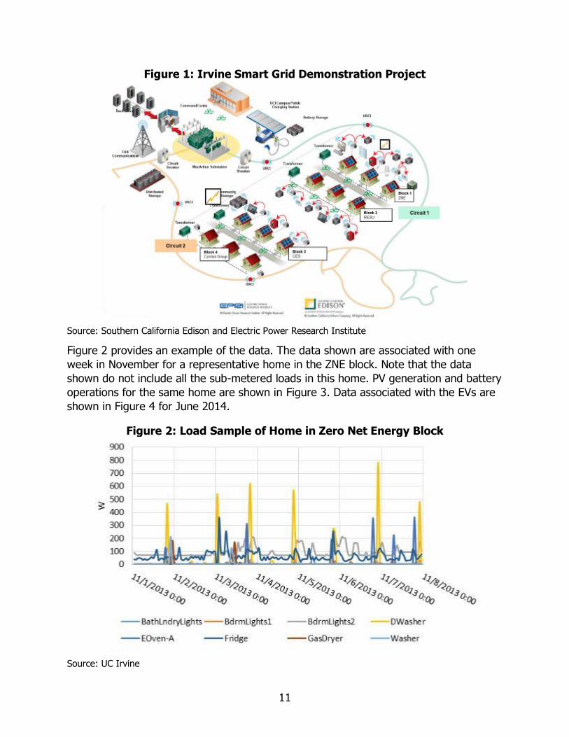
Figure 1: Irvine Smart Grid Demonstration Project
Source: Southern California Edison and Electric Power Research Institute
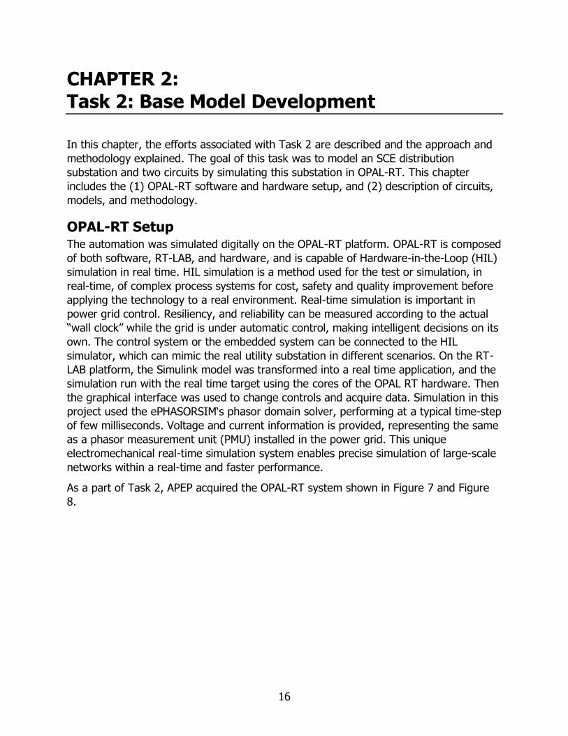
Figure 2 provides an example of the data. The data shown are associated with one
week in November for a representative home in the ZNE block. Note that the data
shown do not include all the sub-metered loads in this home. PV generation and battery
operations for the same home are shown in Figure 3. Data associated with the EVs are
shown in Figure 4 for June 2014.
Figure 2: Load Sample of Home in Zero Net Energy Block
Source: UC Irvine

12
Figure 3: Photovoltaic and Residential Energy Storage Unit Sample Data for Home in ZNE Block
Source: UC Irvine
Figure 4: Electric Vehicle Data for June 2014
Source: UC Irvine

13
Generic Microgrid Controller The main objective of the generic microgrid controller (GMC) project was to design a
controller that will facilitate the deployment of microgrids, be easily adapted to various
microgrid configurations, and reduce up-front engineering costs associated with the
design and development of microgrid controllers. The overarching goal of the GMC
project was to establish controller software specifications that:
• Provide a control structure amenable to accommodating an array of microgrid
configurations and a portfolio of functional requirements.
• Possess a high level architecture that can readily be adopted by commercial
suppliers.
• Support unlimited nesting of conforming microgrid control schemes.
• Integrate into a full-featured Energy Management System (EMS) as a module,
and
• Provide the following features:
o Seamless islanding and reconnection of the microgrid.
o Efficient, reliable, and resilient operation of the microgrid with the
required power quality, whether islanded or grid-connected.
o Existing and future ancillary services to the larger grid.
o The capability for the microgrid to serve the resiliency needs of
participating communities.
o Communication with the electric grid utility as a single controllable entity.
o Increased reliability, efficiency and reduced emissions.
A select set of microgrids, operating a variety of microgrid configurations, served as
“collaborating microgrid partners” in the project and assured thereby that the GMC
developed under this program can readily be applied to microgrids of different sizes,
and equipped with various resources, attributes, and equipment. Collaborating
microgrid partners included the UCI Medical Center), the Port of Los Angeles, Port of
Long Beach, and the Irvine Ranch Water District.
The objectives of the GMC project were achieved in two phases: (Phase I) Research,
Development and Design (Design), and (Phase II) Testing, Evaluation, and Verification
(TEV). In Phase I, specifications were developed for the GMC and a detailed test plan
was established to test the functional requirements of the GMC. The GMC addresses
two core functions, transition and dispatch, as well as several optional higher level
functions such as economic dispatch, and renewable and load forecasting.
For the purposes of Phase II (TEV), the GMC was applied to two microgrids: (1) the 20
MW-class UCI Microgrid (UCIMG), and (2) the 10MW-class UCI Medical Center Microgrid
(UCIMC) using a commercially viable platform (ETAP). Both microgrids and their
components were modeled using the Simulink platform and run on an advanced real-

14
time OPAL-RT hardware-in-the-loop (HIL) simulator. Model simulation results were used
to further inform the development of a controller designed for uninterrupted operation
of the microgrid through events including islanding, reconnection, and internal/external
faults. The simulations demonstrated proof-of-concept, identified the system’s
operational limits, and anchored a test plan for an islanding demonstration of the
UCIMG.
Once the performance of the GMC was established and tested in HIL, the TEV
expanded to include field testing at the UCIMG. UCIMG was then islanded for 75
minutes for a field demonstration which required coordination with UCI Facilities
Management, the UCI Administration, the UCI Office of Design and Construction, the
local utility partner (Southern California Edison), the manufacturer of the UCIMG Co-
Gen (Solar Turbines), and Schweitzer Engineering Laboratories (SEL). During the 75-
minute islanded operation, step loads were added including three 200hp pumps and
campus building loads. In addition, a 500 kW chiller was dropped from the load at
approximately 60-minutes into the excursion. The islanding test demonstrated the
ability of the UCIMG to disconnect from the grid and island, operate in islanded mode
under conditions of load changes, and resynchronize and reconnect to the larger grid.
The two major products of this project were (1) specifications1,2 for a GMC to facilitate
standardization and integration of microgrids, and (2) a successful islanding
demonstration of a community microgrid.
The GMC has two major functions (transition and dispatch) as shown in Figure 5 which
also depicts three levels of control. In this project, the controller adopts the dispatch
function for the two utility 12 kV distribution circuits and, when controlled as single
entities, each circuit is tantamount to a microgrid except for seamless transitions to and
from an islanded mode.
1 Razeghi, G, Gu F, Neal R, Samuelsen S. A Generic Microgrid Controller: Concept, Testing, and Insights.
Applied Energy. 2018; 229:660-71
2 Razeghi G, Neal R, Samuelsen S. Generic Microgrid Controller Specifications. Technical Report to the US
Department of Energy. 2016. http://www.apep.uci.edu/Research/PDF/Microgrid/Generic_Microgrid_Controller_Specifications_Oct_2016
_Razeghi_Neal_Samuelsen_032318.pdf

15
Figure 5: Generic Microgrid Controller Levels of Control
Source: UC Irvine
Figure 6 shows the modular architecture of the GMC as well as device level controller
(load controller (LC), storage controller (SC), and generation controller (GC)). Core level
functions shown in Figure 5 are executed via the Master Microgrid Controller (MMC)
which is the brain of the controller and communicates with device level controllers and
sends them signals/commands. MMC also communicates with higher level functions and
has two major functions: transition, and dispatch as previously discussed.
Figure 6: Generic Microgrid Controller Modular Architecture
Source: UC Irvine
16
CHAPTER 2: Task 2: Base Model Development
In this chapter, the efforts associated with Task 2 are described and the approach and
methodology explained. The goal of this task was to model an SCE distribution
substation and two circuits by simulating this substation in OPAL-RT. This chapter
includes the (1) OPAL-RT software and hardware setup, and (2) description of circuits,
models, and methodology.
OPAL-RT Setup The automation was simulated digitally on the OPAL-RT platform. OPAL-RT is composed
of both software, RT-LAB, and hardware, and is capable of Hardware-in-the-Loop (HIL)
simulation in real time. HIL simulation is a method used for the test or simulation, in
real-time, of complex process systems for cost, safety and quality improvement before
applying the technology to a real environment. Real-time simulation is important in
power grid control. Resiliency, and reliability can be measured according to the actual
“wall clock” while the grid is under automatic control, making intelligent decisions on its
own. The control system or the embedded system can be connected to the HIL
simulator, which can mimic the real utility substation in different scenarios. On the RT-
LAB platform, the Simulink model was transformed into a real time application, and the
simulation run with the real time target using the cores of the OPAL RT hardware. Then
the graphical interface was used to change controls and acquire data. Simulation in this
project used the ePHASORSIM‘s phasor domain solver, performing at a typical time-step
of few milliseconds. Voltage and current information is provided, representing the same
as a phasor measurement unit (PMU) installed in the power grid. This unique
electromechanical real-time simulation system enables precise simulation of large-scale
networks within a real-time and faster performance.
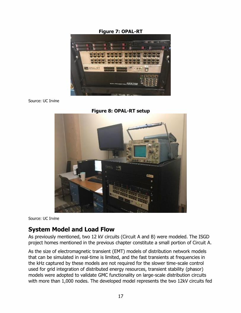
As a part of Task 2, APEP acquired the OPAL-RT system shown in Figure 7 and Figure
8.
17
Figure 7: OPAL-RT
Source: UC Irvine
Figure 8: OPAL-RT setup
Source: UC Irvine
System Model and Load Flow As previously mentioned, two 12 kV circuits (Circuit A and B) were modeled. The ISGD
project homes mentioned in the previous chapter constitute a small portion of Circuit A.
As the size of electromagnetic transient (EMT) models of distribution network models
that can be simulated in real-time is limited, and the fast transients at frequencies in
the kHz captured by these models are not required for the slower time-scale control
used for grid integration of distributed energy resources, transient stability (phasor)
models were adopted to validate GMC functionality on large-scale distribution circuits
with more than 1,000 nodes. The developed model represents the two 12kV circuits fed

18
from an SCE distribution substation as shown in Figure 9. The circuits are constructed
underground. The one-line circuit drawings, provided by SCE, were used to develop
models on MATLAB Simulink. The ISGD project blocks were modeled in detail in the
circuit. The Zero Net Energy (ZNE) block was modeled as a smart-home to achieve zero
net energy with 4kW rooftop solar photovoltaic (PV) panels and 4kW/10kWh battery
storage along with electric vehicle charging equipment and other various dispatchable
loads (such as HVAC and smart appliances including smart fridge). Also the Residential
Energy Storage Unit (RESU) block and the Community Energy Storage (CES) block were
modeled with the same equipment but with 4kW/10kWh battery storage in each home
for the RESU block and a 25kW/50kWh battery near the distribution transformer for 9
homes of the CES block. The load associated with the ZNE block is adjusted to reflect
the energy efficiency measures implemented in these homes.
Figure 9: Circuit Model
Source: UC Irvine
The rooftop solar PV array model was shared by the OPAL-RT-project partner. This PV
model has insolation, temperature, 3-phase grid voltage and reference real and reactive
power as inputs, and creates 3-phase current injections as its output. The current
injections can either be in the form of sinusoidal waveforms for EMT simulation or as
current phasors (magnitude and angle) for TS simulation. The model uses a single ideal
diode structure for the DC output of the PV cells, the voltage being a function of
insolation and temperature. A perturb-and-observe MPPT (maximum power point
tracking) controller was used to maintain PV power output at peak power. The next
stage of the model is a boost converter followed by a voltage source converter to create
the desired AC output as commanded by the real and reactive power commands. A
curtailment function was included to handle situations when the commanded real and

19
reactive power exceeds the power output of the PV cells. Different types of PV brand
and model can be selected and set the parallel strings and series connected modules
per string for the capacity of the PV. Each PV array was set to deliver a maximum of 3.6
kW at 1000W/m² sun irradiance. The PV array was then connected to a boost converter
with the maximum power point tracking (MPPT) controller to track the maximum power
point and boost the voltage. Then a DC-AC inverter was connected to switch the DC
voltage to the needed AC voltage. This model is included in Figure 10.
Figure 10: Home Model with Photovoltaic and Battery
Source: UC Irvine
The battery was modeled to be controlled with the current, and controlled to operate at
different charge and discharge modes by the controller which was developed with the
Generic Microgrid Controller specifications in Task 4. For the simulation of the home
model, the current from the PV was fed into the battery to charge and the battery
discharged when PV generation was zero. Similarly, the battery for the CES block
charged from the grid next to the transformer and discharged when the total load on
the transformer was larger than 25kVA. All the home models were modeled with
dispatchable loads which could be switched on and off or adjusted to a required
amount. This was also a control point for the controller. A dynamic load block was
modeled as shown in Figure 11 and connected in the home block to enable this feature.

20
Figure 11: Dynamic Load Model
Source: UC Irvine
The control block was modeled as well. This block does not include any distributed
energy resources, renewable generation, dispatchable loads, and electric vehicles. A
total of 4 blocks and 32 homes are modeled as the ISGD project and the rest of the
loads are identified as lumped loads throughout the circuit. In Task 3, various scenarios
will be developed and the penetration of renewables and DERs will be increased on
these circuits to study their impacts. In addition ZNE homes will be simulated
throughout the circuit along with other technologies.
The existing CYME models were imported into the OPAL-RT ePHASORsim environment
for real-time simulation. Analysis of the CYME file indicated that specific transformer
models are not currently supported in the import functionality of ePHASORsim. These
models need to be added to CYME-to-ePHASORsim converter developed by OPAL-RT
and work is currently on-going in this regard.
Once the import functionality of the transformer models in the network was addressed,
namely the model was configured to allow real-time simulation of the network with
controllable loads and distributed energy resources at various points in the network.
The model was also set up to communicate with the GMC using standard
communication protocols such as IEC 61850 or DNP3.
Load Flow Analysis
With the as-is circuit model, a power flow study was performed using the CYME
software. The voltage drop calculation technique was used which computes the
voltages and power flows at every node of the model within 10 or less iterations and
the load profiles are preset to values used from SCE. By running the load flow analysis,
results for the 2 circuits are shown below. The abnormal over and under voltages were
within the +-5% limits (Tables 1 through 3). Figure 12 shows the circuit lines with the
voltage unbalance.
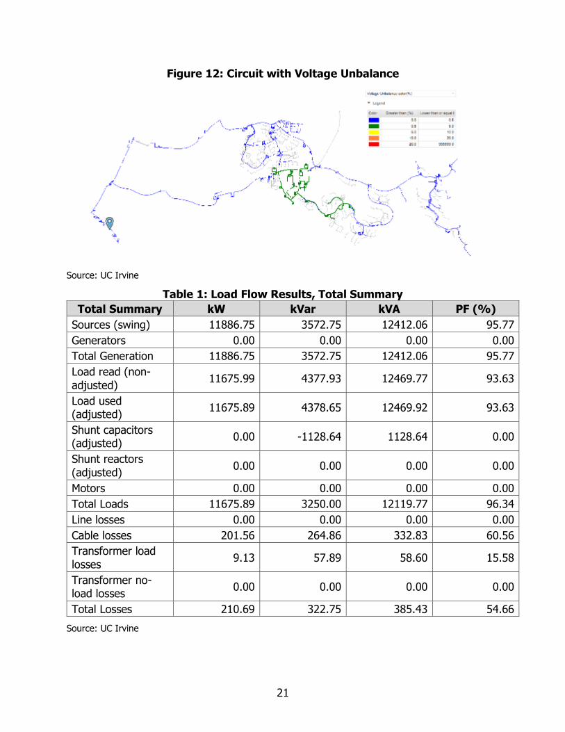
21
Figure 12: Circuit with Voltage Unbalance
Source: UC Irvine
Table 1: Load Flow Results, Total Summary
Total Summary kW kVar kVA PF (%)
Sources (swing) 11886.75 3572.75 12412.06 95.77
Generators 0.00 0.00 0.00 0.00
Total Generation 11886.75 3572.75 12412.06 95.77
Load read (non-
adjusted) 11675.99 4377.93 12469.77 93.63
Load used (adjusted)
11675.89 4378.65 12469.92 93.63
Shunt capacitors (adjusted)
0.00 -1128.64 1128.64 0.00
Shunt reactors
(adjusted) 0.00 0.00 0.00 0.00
Motors 0.00 0.00 0.00 0.00
Total Loads 11675.89 3250.00 12119.77 96.34
Line losses 0.00 0.00 0.00 0.00
Cable losses 201.56 264.86 332.83 60.56
Transformer load
losses 9.13 57.89 58.60 15.58
Transformer no-load losses
0.00 0.00 0.00 0.00
Total Losses 210.69 322.75 385.43 54.66
Source: UC Irvine

22
Table 2: Load Flow Results, Abnormal Conditions
Abnormal Conditions
Phase Count Worst Condition Value
A 2 Circuit 12kV 127.61%
Overload B 2 Circuit 12kV 123.39%
C 2 Circuit 12kV 123.23
9.13 A 0 5545961:P5545961-XFO 99.57 %
Under-
Voltages B 0
5526185:B5526185-XFO 99.70 %
C 0 5510839:P5510839-XFO 100.50 %
A 0 GS1350-3$15373 103.92 %
Over-Voltages B 0 GS1350-3$15373 103.92 %
C 0 GS1350-3$15373 103.92 %
Source: UC Irvine
Table 3: Load Flow Results, Annual Cost of System Losses
Annual Cost of System Losses kW MWh/year k$/year
Line losses 0.00 0.00 0.00
Cable losses 201.56 1765.66 176.57
Transformer load losses 9.13 79.96 8.00
Transformer no-load losses 0.00 0.00 0.00
Total losses 210.69 1845.63 184.56
Source: UC Irvine

23
CHAPTER 3: Task 3: Scenario Development
This chapter outlines the efforts associated with Task 3 of the project entitled Scenario
Development. The goal of this task was to develop a set of future viable scenarios to be
assessed using the models and the controller based on the GMC specifications.
This chapter provides an overview of the scenarios and tests to be performed. The
scenarios included in this project cover:
• The various technologies to be added as DER to the circuits under study
• The various smart grid technologies to further enhance controllability of the
assets
• The demand response strategies to further optimize the operations
• The maximum DER/renewable penetration that the circuits can handle
• The impacts of DER on the distribution circuit if the maximum penetration is
surpassed
• Viable future scenarios to be further assessed using modeling
Methodology Scenarios identified in this chapter were executed in accordance with detailed test
procedures. Each procedure will:
• Define the purpose of the test
• Identify task objective satisfied by the test
• Describe system test conditions including initial conditions
• Identify parameters to be monitored
• Describe steps of the test
• Identify expected results
• Record actual results
• Record any deviations from test steps
• Perform required post-processing (e.g. emissions and efficiency calculations)
The template used for each category of scenarios and tests is shown in Template A-1 in
Appendix A.3 This procedure and methodology has been previously used by APEP in the.
DOE GMC project which resulted in successful testing and development of the GMC.
3 GMC Test Plan, Advanced Power and Energy Program, Report to US. DOE, April 2016
24
As previously mentioned, the GMC has two major functions (transition and dispatch) as
shown in Figure 5.4 The majority of the scenarios assessed in this project (Task 4)
focused on the dispatch function in which resources were dispatched in the most
economic manner (economic optimization).
Scenarios were divided in four main groups: high renewable penetration, energy
storage, demand response, and circuit-independent. In each group, a variable (e.g.
renewable penetration) was changed in the circuit and the simulations were done. The
results of the simulation include the load flow in the circuits, cost of generation, and the
operation of DERs. Emissions and efficiency were calculated after the simulations. Cases
were repeated for different initial and operating conditions to cover different situation
(such as winter vs summer and cloudy vs sunny days).
For the DERs, solar PV and battery energy storage were determined to be the most
suitable options for the circuits under study. Conventional generators were avoided in
order to reduce the environmental impacts. In the demand response scenarios, it was
assumed that homes are equipped with smart appliances and energy management
systems which can respond to demand response requests. Plug-in electric vehicles were
also used in these scenarios as controllable load thus the charger should be able to
communicate with the controller.
For the base case, it was assumed that the two circuits have a PV penetration equal to
that of the ISGD blocks. The load associated with one of the circuits is shown in Figure
13 for the week of 11/10-11/16 2014. Note that the horizontal axis shows the sample
number and not time. These data are recorded at 30 samples per second rate using
synchrophasors located at the substation. In the base case, it was further assumed that
the electricity demand is rigid and not controllable.
4 Generic Microgrid Controller Specification, Advanced Power and Energy Program, Report to US DOE,
October 2016

25
Figure 13: Real Power (MW)- Circuit A
Source: UC Irvine
Scenarios
Scenario 1: High Renewable Penetration
In these scenarios, solar PV penetration in the circuits was increased from the base
case to 100%. Based on previous APEP research conducted under a California Solar
Initiative (CSI), it was expected that 100% PV penetration is not feasible due to
intermittency and instability introduced by PV5. Thus, as the PV penetration increases
and the simulations repeated, a threshold for the PV penetration on the circuits was
established. Studying the scenarios with higher penetration helped identify the issues
(system constraints), impacts, and solutions to achieve higher penetrations and
increase the threshold. The procedures for these tests are shown in Template A-2 in
Appendix A. For the electricity not generated locally and imported from the utility, SCE
tariffs and prices were used. For PV, the LCOE was used and calculated from CEC Cost
of Generation Model.
Note that after establishing the maximum PV penetration, another feasibility check was
conducted to ensure that there is enough roof space or open spaces on the circuits to
install this amount of solar PV.
5 Samuelsen, S.; Brouwer, J. Development and analysis of a progressively smarter distribution system,
Final Report, Submitted to CSI RD&D Program Administrator

26
Scenario 2: Energy Storage
In these scenarios, battery energy storage was added as another DER to the circuits
with maximum PV penetration to assess its impact on the circuits. Furthermore, the PV
penetration was increased on these circuits to determine whether or not the addition of
energy storage helps to increase the feasible PV penetration in general. These scenarios
were divided into the following three groups modeled after ISGD project:
1. RESU (Residential Energy Storage Unit), in which each household has a
4kW/10kWh battery energy storage. In these scenarios, the “mode” (e.g. PV
Capture, peak-shaving) of the battery operation was controlled and set by the
GMC at the substation. See Template A-3 in Appendix A for the details.
2. CES (Community Energy Storage), in which each block (corresponding to each
transformer) is equipped with a 25kW/50kWh energy storage. The operation of
these resources was controlled by the GMC. See Template A-4 in Appendix A for
the details.
3. Substation (or Circuit) battery: In these cases, a bigger energy storage
(2MW/500kWh) was simulated at the substation to support the operation of the
two circuits under study. The data collected during ISGD project for such a
battery was used. (Note that such a battery existed on one of circuits during
ISGD but has since been moved to another location). See Template A-5 in
Appendix A. Directed by the results of the simulation, energy storage of different
sizes were also simulated.
4. Scenario 3: Demand Response
These scenarios built upon the previous simulations. It was assumed that the system
was equipped with energy storage and the corresponding maximum PV penetration for
that type of storage determined in Group B simulations. The scenarios were divided in
two groups:
1. HVAC and smart appliances: In these scenarios, it was assumed that the homes
are equipped with HVAC and smart appliances that can participate in demand
response, and with energy management systems (EMS) communicating with the
GMC to respond to signals. Details are provided in Template A-6 in Appendix A.
2. Plug-in electric vehicles (PEV): In these scenarios, the homes were equipped
with smart appliances and HVAC as the previous group, and a plug-in electric
vehicle was allocated to each household. It is further assumed that the chargers
were capable of accepting and responding to signals. Details are provided in
Template A-7 in Appendix A.
For these scenarios, initially, the current demand response programs and incentives
offered by SCE were used.

27
Scenario 4: Circuit-Independent
In this scenario, a fuel cell was modeled at the substation to serve as a grid resource in
order to fully support the load of the system without having to import any electricity
from the grid. Thus, all the required generation was produced locally using DERs and
with the help of controllable loads. This is similar to operation of a microgrid in islanded
mode (dispatch while islanded) and thus the objective was not to meet the load at
minimum cost but to meet the load without import. Note that transition from grid
connected to islanded and vice versa and the transients associated with transition were
not studied in this project. Several options were simulated under this scenario. Details
are provided in Template A-8 in Appendix A.

28
CHAPTER 4: Task 4: Controller Development
For the purposes of this project, the GMC specifications were used to establish the
requirements and functionalities of the controller that was simulated at the substation
to enable substation automation and control. A schematic of the controller and three
levels of controls are shown in Figure 14 as well as device controllers corresponding to
LC, SC, and GC in GMC architecture (Figure 6). Note that core level functions are
executed via the MMC. Since transitioning to islanded mode is not included in this
project, the breakers are not included in the controls. Utility signals and requests, as
well as system status data (including load data) were inputs, and the outputs included
signals to the DERs in the two circuits. The DERs on the two circuits included demand
response, rooftop photovoltaics and different scales of battery energy storage systems
that include combinations of residential energy storage units (RESU), community energy
storage (CES), and larger circuit battery energy storage in different scenarios. In one of
the scenarios, a fuel cell was simulated at the substation as well.
The batteries had a local (device) control mechanism built in as a model and operated
as either (1) residential energy storage units (RESUs) with PV-capture and time-base
load shifting modes, or (2) community energy storage (CES) with permanent load-
shifting and load-limiting modes.. These modes are described in details in Section 0 and
0 of this document.
The mode of operation was determined by the controller. This was done to avoid
sending set-points to individual DERs from the controller, which results in a large
number of variables and is impractical for the utility or operator to control thousands of
DERs across the grid. The fuel cell operated in either a base-loading or load-following
mode determined by the controller, and the demand response signal was sent by the
controller to loads’ local controller based on the utility request or the need to balance
load and generation. Load controllers included the local controller on electric vehicle
service equipment (EVSEs) associated with plug-in electric vehicles (PEVs), and energy
management system (EMS) of the customer.
the following sections present the local and substation controllers are explained, and
their assumptions, logic, strategy, and resulting outcomes.

29
Figure 14: Controller Schematic and Levels of Control
Source: UC Irvine
Device (Local) Controllers
Residential Energy Storage Unit
Model Description
The residential energy storage units (RESUs) were comprised of a PV array and a
battery connected to a single inverter. The inputs included the home electricity load, PV
array output, and mode of operation. The outputs included inverter power output and a
measurement port containing the load power demand, the PV array output power, the
battery output power, the inverter output power and the battery state of charge (SOC).
The RESU component and its mask are shown in Figure 15 to Figure 17. The “Power”
tab contains the power stage parameters, namely inverter rated power in kW, battery
rated capacity in kWh, battery initial SOC in percentage and roundtrip efficiency in

30
percentage. The “Control” tab contains the parameters pertaining to the control stage
of the system, namely admissible battery SOC range in percentage, maximum charging
power during night time in kW and charging/discharging time interval in hours. The
RESU output power is calculated based on the load demand, PV output and battery
charge/discharge power, and is further limited by the inverter rated power. The
available battery energy is dependent on its SOC.
Figure 15: Residential Energy Storage Unit Component
Source: UC Irvine
Figure 16: Residential Energy Storage Unit Component Mask, Power Tab
Source: UC Irvine

31
Figure 17: Residential Energy Storage Unit Component Mask, Control Tab
Source: UC Irvine
Model Control Validation
Two operation modes were modeled for the RESU: PV capture and Time-based load
shifting. The control logic for each mode was designed and validated by comparing the
simulation results to the data and the field experiment results from the ISGD project.
When operating in PV capture mode, the battery output follows its power set-point,
which is the difference between the PV output and the load demand, as long as the
battery SOC remains within the acceptable predefined range. The battery charges when
the PV output is more than the load demand and discharges when it is less. If the
battery reaches its maximum SOC and the load demand is met, the surplus PV power is
fed back to the grid. Similarly, if it reaches its minimum SOC and the load demand is
not met, the grid has to provide the required power. Figure 18 presents the simulation
results for a 24 hours period running the RESU in PV capture mode. The load and PV
profiles were taken from the ISGD data, the battery initial SOC was set to 50% and the
admissible SOC range was set to 20%-90%. Negative power means the battery was
charging.

32
Figure 18: Residential Energy Storage Unit Simulation Results, Photovoltaic Capture Mode
Source: UC Irvine
When operating in time-based load shifting mode, the battery charges and discharges
during specified time ranges. The charging power set-point was fixed to the specified
“Maximum charging power” value, whereas the discharging power was calculated based
on the battery SOC and the duration of the specified discharge cycle, so that the
battery reaches its minimum SOC at the end of the cycle. The discharging power is also
limited by the inverter rating and PV output power. Figure 19 presents the simulation
results for a 24 hours period running the RESU in Time-based load shifting mode. The
load and PV profiles were taken from the ISGD data, the battery initial SOC was set to
50% and the admissible SOC range was set to 20%-90%. Negative power means the
battery was charging.

33
Figure 19: Residential Energy Storage Unit Simulation Results, Time-Based Load Shifting Mode
Source: UC Irvine
Community Energy Storage
Model Description
The community energy storage (CES) units were installed near the distribution
transformers and supply all the customers downstream. The inputs were the total load
power and PV output power from all the homes downstream as well as the mode of
operation. The outputs were the inverter power output and a measurement port
containing the total load power demand and total PV output power of the block, the
CES output power and the battery SOC.
The CES component and its mask are shown in Figure 20 to Figure 23. The “Power” tab
contains the power stage parameters, namely inverter rated power in kW, rated
capacity of the battery in kWh, battery initial SOC in percentage, roundtrip efficiency in
percentage and admissible battery SOC range in percentage. The “Permanent Load

34
Figure 20: Community Energy Storage Component
Source: UC Irvine
Figure 21: Community Energy Storage Component Mask, Power Tab
Source: UC Irvine
Shifting mode (PLS)” tab contains the parameters pertaining to the CES control stage
when operating in PLS mode, namely charging and discharging power set-point in kW,
charging and discharging power slope limit in kW/h and time intervals for the charging
and discharging cycles. The “Load Limiting mode” tab contains parameters pertaining to
the CES control stage when operating in Load Limiting mode, namely the load and
generation limits in kW. The CES output power is calculated based on the total

35
residential block load demand and PV output power. It is limited by the CES inverter
rated power and also dependent on the battery SOC.
Figure 22: Community Energy Storage Component Mask, Permanent Load Shifting Mode Tab
Source: UC Irvine

36
Figure 23: Community Energy Storage Component Mask, Load Limiting Mode
Source: UC Irvine
Model Control Validation
Two operation modes were modeled for the CES: Permanent Load Shifting (PLS) and
Load Limiting. The control logic for each mode was designed and validated by
comparing the simulation results to the data collected from the field experiments in the
ISGD project. When operating in PLS mode, the battery charges and discharges during
specific time windows that are determined by the operator. The charging power set-
point was fixed to the specified “Charging power set-point,” whereas the discharging
power was fixed to the specified “Discharging power set-point”. Figure 24 presents the
simulation results for a 24 hours period running the CES in Permanent Load Shifting
mode. The load and PV profiles were taken from the CES block ISGD data, the battery
initial SOC was set to 50% and the admissible SOC range was set to 20%-90%.
Negative power means the battery was charging.

37
Figure 24: Community Energy Storage Simulation Results, Permanent Load Shifting Mode
Source: UC Irvine
When operating in Load Limiting mode, the CES charges and discharges as necessary,
were subject to its capacity limits, to limit both imported and exported power at the
distribution transformer to the specified set-points. Figure 25 presents the simulation
results for a 24 hours period running the CES in Load Limiting mode. The load and PV
profiles were taken from the CES block ISGD data, the battery initial SOC was set to
50% and the admissible SOC range is set to 20%-90%. Negative power means the
battery was charging.

38
Figure 25: Community Energy Storage Simulation Results, Load Limiting Mode
Source: UC Irvine
Circuit Battery
Model Description
The circuit battery energy storage model was based on the community energy storage
model. Installed near the substation, the battery supplied all the customers
downstream. Its inputs were the total load power from all the customers downstream
as well as the mode of operation. The outputs included the inverter power output and a
measurement port containing the total load power demand, the output power and the
battery SOC (see Figure 26).
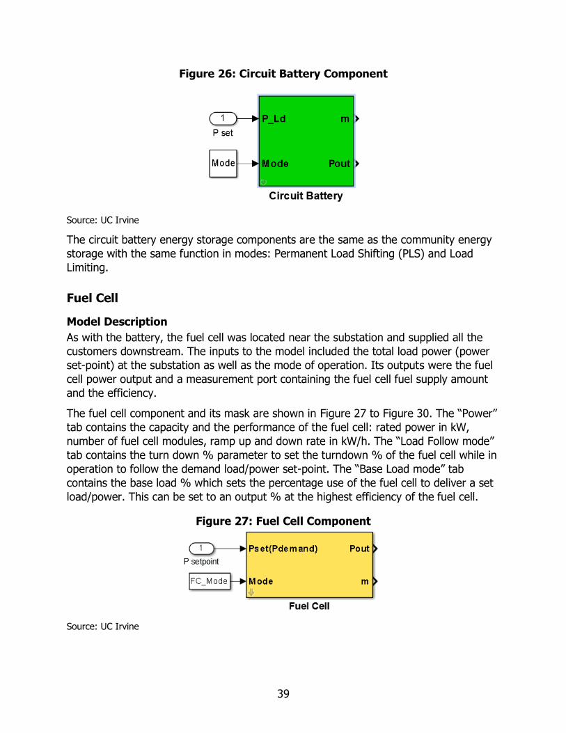
39
Figure 26: Circuit Battery Component
Source: UC Irvine
The circuit battery energy storage components are the same as the community energy
storage with the same function in modes: Permanent Load Shifting (PLS) and Load
Limiting.
Fuel Cell
Model Description
As with the battery, the fuel cell was located near the substation and supplied all the
customers downstream. The inputs to the model included the total load power (power
set-point) at the substation as well as the mode of operation. Its outputs were the fuel
cell power output and a measurement port containing the fuel cell fuel supply amount
and the efficiency.
The fuel cell component and its mask are shown in Figure 27 to Figure 30. The “Power”
tab contains the capacity and the performance of the fuel cell: rated power in kW,
number of fuel cell modules, ramp up and down rate in kW/h. The “Load Follow mode”
tab contains the turn down % parameter to set the turndown % of the fuel cell while in
operation to follow the demand load/power set-point. The “Base Load mode” tab
contains the base load % which sets the percentage use of the fuel cell to deliver a set
load/power. This can be set to an output % at the highest efficiency of the fuel cell.
Figure 27: Fuel Cell Component
Source: UC Irvine

40
Figure 28: Fuel Cell Component Mask, Power Tab
Source: UC Irvine
Figure 29: Fuel Cell Component Mask, Base Load Mode
Source: UC Irvine

41
Figure 30: Fuel Cell Component Mask, Load Limiting Mode
Source: UC Irvine
Model Control Validation
Two operation modes were modeled for the fuel cell: Base Load and Load Following.
When operating in Base Load mode, the fuel cell will supply constant power which is
specified with the “base load %” parameter. It will act as a base load supplier at the
substation. Figure 31 shows the result of the fuel cell operating at base load mode; the
parameters were set to max capacity of 6MW and base load percentage to 50. The fuel
cell outputted 3MW constantly throughout a day.
When operating in the load-following mode, the fuel cell outputted power according to
the power set point/power demand. The fuel cell followed the load within its power
capacity and ramp up and down constraints. Figure 32 shows the result of the load
following mode. With the same capacity parameters, 50% turndown set point and
10kW/h and -20kW/h ramp rates, the fuel cell followed the load subject to its
operational constraints.

42
Figure 31: Fuel Cell Simulation at the Substation – Base Load Mode Result
Source: UC Irvine
Figure 32: Fuel Cell Simulation at the Substation - Load Follow Mode Result
Source: UC Irvine
Demand Response
Two types of demand response (DR) signals were sent from the controller: 1) HVAC
and smart appliance demand response, and 2) Plug-in electric vehicles (PEV). The
demand response signal was based on the utility request or it was initiated when
physical constraints of the system are violated. The measurements from the two circuits

43
were inputs to the controller and the controller detected when there is abnormal
voltage, transmission overflow and transformer overload.
1. HVAC and smart appliances: The demand response signal for home appliances
including the HVAC was sent to the load on the circuit. Figure 33 shows the
result of a demand response sent to a home during 6am to 1pm and again at
5pm to 10pm. The capacity of load reduction was obtained from the ISGD
project’s demand response experiments. In practice, this signal will be sent to
the energy management system of the residence, and the EMS will make the
decision on how to meet the requested DR. EMS and its details are outside the
scope of the current project.
Figure 33: Demand Response – Result
Source: UC Irvine
2. Plug-in electric vehicles (PEV): Demand response was accomplished on the
electric vehicle supply equipment (EVSE). With a PEV in each household, a
demand response signal was sent from the controller to adjust the charging rate
or to turn on and off the EVSE. Figure 34 shows the EVSE charger mask in the
model. The designed EVSE logic was based on the ISGD report description and
test results and was adapted to fit desired behavior. From midnight to 7am, the
EVSE rejected DR events to ensure that the PEV reached full charge in the
morning. From 7am to midnight, the EVSE accepted DR events, depicted as
“Requested ChargeRate%” in Figure 34, corresponding to changes in the
charging rate. Figure 35 presents the EVSE simulation results for one day. The
demand response event was selected to test the logic and control. In the result,
the EVSE power output corresponding to the DR charge rate % change can be
seen. Note that from 7am-10am, the PEV was not connected to the charger (i.e.

44
Charging status=0), thus it could not respond to the Requested ChargeRate. Also
note, that in these simulations, whenever the PEV was not available or not
connected to the charger (i.e. Charging status=0), the SOC was set to 0 due to
lack to communication between the EVSE and the vehicle. In these situations the
EVSE could not respond to the DR request (Requested ChargeRate%). When the
PEV was reconnected to the EVSE, the actual SOC was then communicated to
the local controller. For example, at 10am the PEV was connected to the EVSE
and the actual SOC was read. The reading was lower than the reading at 7am,
indicating that the PEV was driven between these hours
Figure 34: Electric Vehicle Supply Equipment Mask Model
Source: UC Irvine
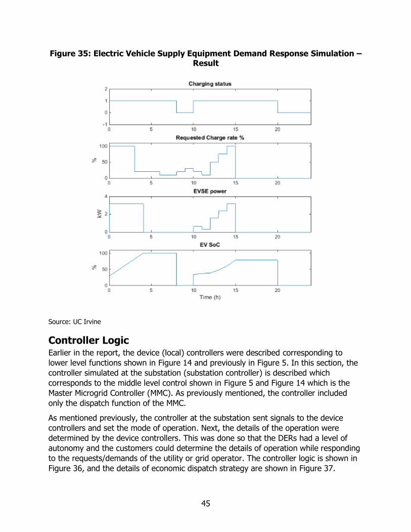
45
Figure 35: Electric Vehicle Supply Equipment Demand Response Simulation – Result
Source: UC Irvine
Controller Logic Earlier in the report, the device (local) controllers were described corresponding to
lower level functions shown in Figure 14 and previously in Figure 5. In this section, the
controller simulated at the substation (substation controller) is described which
corresponds to the middle level control shown in Figure 5 and Figure 14 which is the
Master Microgrid Controller (MMC). As previously mentioned, the controller included
only the dispatch function of the MMC.
As mentioned previously, the controller at the substation sent signals to the device
controllers and set the mode of operation. Next, the details of the operation were
determined by the device controllers. This was done so that the DERs had a level of
autonomy and the customers could determine the details of operation while responding
to the requests/demands of the utility or grid operator. The controller logic is shown in
Figure 36, and the details of economic dispatch strategy are shown in Figure 37.
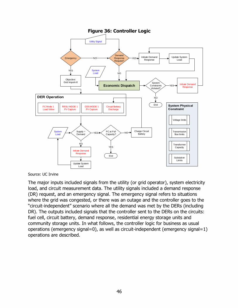
46
Figure 36: Controller Logic
Source: UC Irvine
The major inputs included signals from the utility (or grid operator), system electricity
load, and circuit measurement data. The utility signals included a demand response
(DR) request, and an emergency signal. The emergency signal refers to situations
where the grid was congested, or there was an outage and the controller goes to the
“circuit-independent” scenario where all the demand was met by the DERs (including
DR). The outputs included signals that the controller sent to the DERs on the circuits:
fuel cell, circuit battery, demand response, residential energy storage units and
community storage units. In what follows, the controller logic for business as usual
operations (emergency signal=0), as well as circuit-independent (emergency signal=1)
operations are described.
Emergency
Utility Signal
Voltage limits
Transmission flow limits
Transformer Capacity
NO
System Constraints Violated?
End
NO
Initiate Demand Response
YES
NO
YESInitiate Demand
ResponseUpdate System
Load
Substation Limits
Demand Response Request?
Objective: Grid Import=0
Economic Dispatch
YES
FC Mode 1 Load follow
Initiate Demand Response
Supply = Demand
Circuit Battery Discharge
NO
RESU MODE 1 PV Capture
CES MODE 1 PV Capture
System Load
YES
Update System Load
System Load
FC at Full Capacity?
End
YES
Charge Circuit Battery
NO
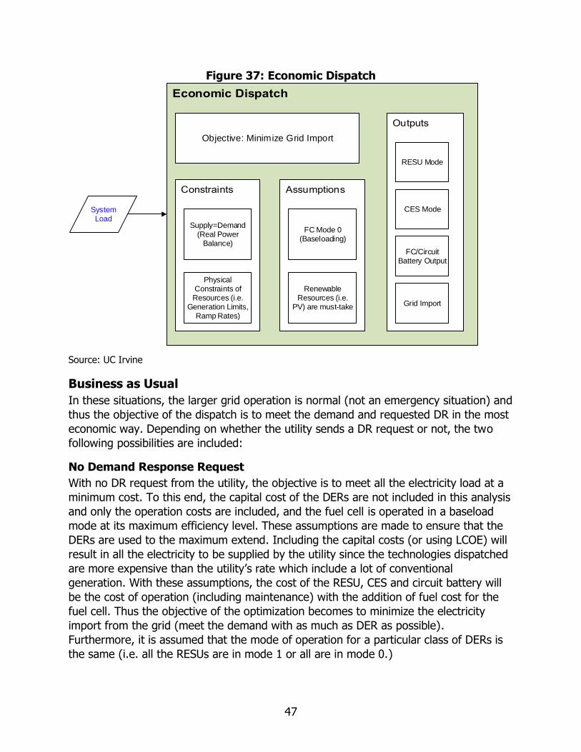
47
Figure 37: Economic Dispatch
Source: UC Irvine
Business as Usual
In these situations, the larger grid operation is normal (not an emergency situation) and
thus the objective of the dispatch is to meet the demand and requested DR in the most
economic way. Depending on whether the utility sends a DR request or not, the two
following possibilities are included:
No Demand Response Request
With no DR request from the utility, the objective is to meet all the electricity load at a
minimum cost. To this end, the capital cost of the DERs are not included in this analysis
and only the operation costs are included, and the fuel cell is operated in a baseload
mode at its maximum efficiency level. These assumptions are made to ensure that the
DERs are used to the maximum extend. Including the capital costs (or using LCOE) will
result in all the electricity to be supplied by the utility since the technologies dispatched
are more expensive than the utility’s rate which include a lot of conventional
generation. With these assumptions, the cost of the RESU, CES and circuit battery will
be the cost of operation (including maintenance) with the addition of fuel cost for the
fuel cell. Thus the objective of the optimization becomes to minimize the electricity
import from the grid (meet the demand with as much as DER as possible).
Furthermore, it is assumed that the mode of operation for a particular class of DERs is
the same (i.e. all the RESUs are in mode 1 or all are in mode 0.)
Objective: Minimize Grid Import
Supply=Demand(Real Power
Balance)
Physical Constraints of Resources (i.e.
Generation Limits, Ramp Rates)
FC Mode 0 (Baseloading)
Renewable Resources (i.e.
PV) are must-take
RESU Mode
CES Mode
FC/Circuit Battery Output
Grid Import
System Load
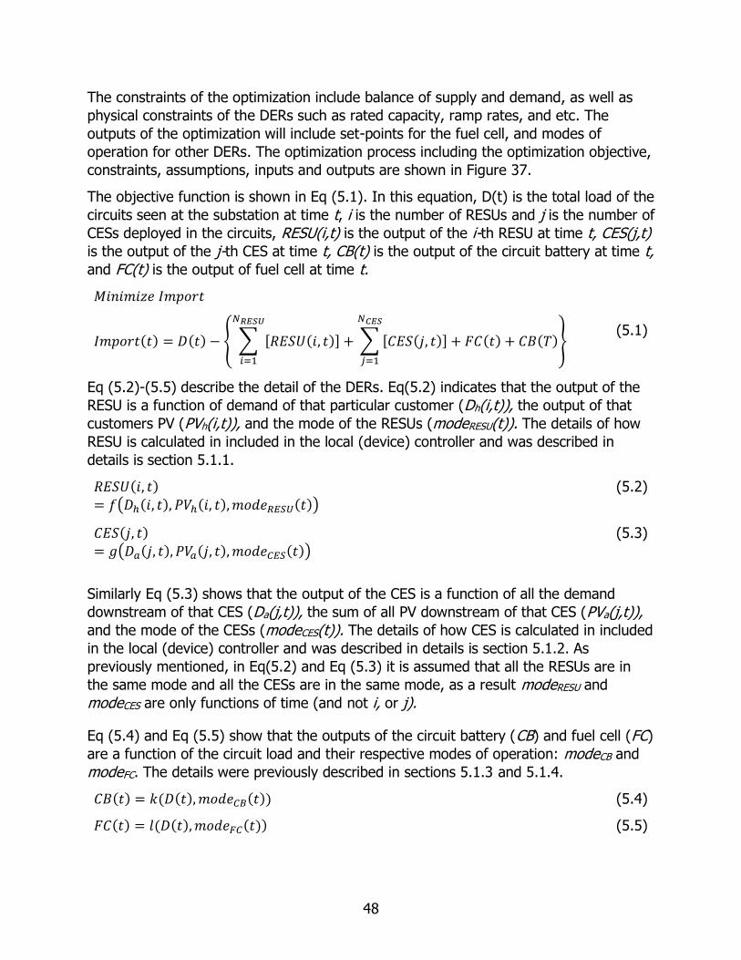
48
The constraints of the optimization include balance of supply and demand, as well as
physical constraints of the DERs such as rated capacity, ramp rates, and etc. The
outputs of the optimization will include set-points for the fuel cell, and modes of
operation for other DERs. The optimization process including the optimization objective,
constraints, assumptions, inputs and outputs are shown in Figure 37.
The objective function is shown in Eq (5.1). In this equation, D(t) is the total load of the
circuits seen at the substation at time t, i is the number of RESUs and j is the number of
CESs deployed in the circuits, RESU(i,t) is the output of the i-th RESU at time t, CES(j,t) is the output of the j-th CES at time t, CB(t) is the output of the circuit battery at time t, and FC(t) is the output of fuel cell at time t.
𝑀𝑖𝑛𝑖𝑚𝑖𝑧𝑒 𝐼𝑚𝑝𝑜𝑟𝑡
𝐼𝑚𝑝𝑜𝑟𝑡(𝑡) = 𝐷(𝑡) − { ∑ [𝑅𝐸𝑆𝑈(𝑖, 𝑡)]
𝑁𝑅𝐸𝑆𝑈
𝑖=1
+ ∑ [𝐶𝐸𝑆(𝑗, 𝑡)] + 𝐹𝐶(𝑡) + 𝐶𝐵(𝑇)
𝑁𝐶𝐸𝑆
𝑗=1
}
(5.1)
Eq (5.2)-(5.5) describe the detail of the DERs. Eq(5.2) indicates that the output of the
RESU is a function of demand of that particular customer (Dh(i,t)), the output of that
customers PV (PVh(i,t)), and the mode of the RESUs (modeRESU(t)). The details of how
RESU is calculated in included in the local (device) controller and was described in
details is section 5.1.1.
𝑅𝐸𝑆𝑈(𝑖, 𝑡)
= 𝑓(𝐷ℎ(𝑖, 𝑡), 𝑃𝑉ℎ(𝑖, 𝑡), 𝑚𝑜𝑑𝑒𝑅𝐸𝑆𝑈(𝑡)) (5.2)
𝐶𝐸𝑆(𝑗, 𝑡)
= 𝑔(𝐷𝑎(𝑗, 𝑡), 𝑃𝑉𝑎(𝑗, 𝑡), 𝑚𝑜𝑑𝑒𝐶𝐸𝑆(𝑡))
(5.3)
Similarly Eq (5.3) shows that the output of the CES is a function of all the demand
downstream of that CES (Da(j,t)), the sum of all PV downstream of that CES (PVa(j,t)), and the mode of the CESs (modeCES(t)). The details of how CES is calculated in included
in the local (device) controller and was described in details is section 5.1.2. As
previously mentioned, in Eq(5.2) and Eq (5.3) it is assumed that all the RESUs are in
the same mode and all the CESs are in the same mode, as a result modeRESU and modeCES are only functions of time (and not i, or j).
Eq (5.4) and Eq (5.5) show that the outputs of the circuit battery (CB) and fuel cell (FC)
are a function of the circuit load and their respective modes of operation: modeCB and
modeFC. The details were previously described in sections 5.1.3 and 5.1.4.
𝐶𝐵(𝑡) = 𝑘(𝐷(𝑡), 𝑚𝑜𝑑𝑒𝐶𝐵(𝑡)) (5.4)
𝐹𝐶(𝑡) = 𝑙(𝐷(𝑡), 𝑚𝑜𝑑𝑒𝐹𝐶(𝑡)) (5.5)
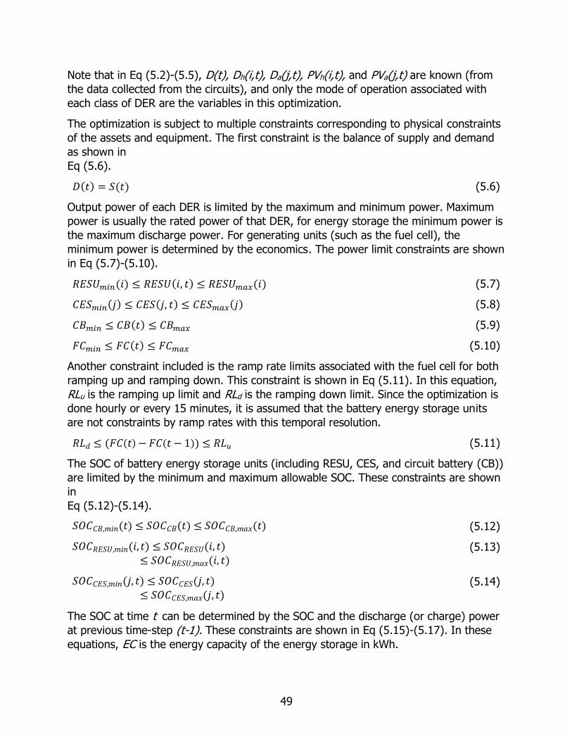
49
Note that in Eq (5.2)-(5.5), D(t), Dh(i,t), Da(j,t), PVh(i,t), and PVa(j,t) are known (from
the data collected from the circuits), and only the mode of operation associated with
each class of DER are the variables in this optimization.
The optimization is subject to multiple constraints corresponding to physical constraints
of the assets and equipment. The first constraint is the balance of supply and demand
as shown in
Eq (5.6).
𝐷(𝑡) = 𝑆(𝑡) (5.6)
Output power of each DER is limited by the maximum and minimum power. Maximum
power is usually the rated power of that DER, for energy storage the minimum power is
the maximum discharge power. For generating units (such as the fuel cell), the
minimum power is determined by the economics. The power limit constraints are shown
in Eq (5.7)-(5.10).
𝑅𝐸𝑆𝑈𝑚𝑖𝑛(𝑖) ≤ 𝑅𝐸𝑆𝑈(𝑖, 𝑡) ≤ 𝑅𝐸𝑆𝑈𝑚𝑎𝑥(𝑖) (5.7)
𝐶𝐸𝑆𝑚𝑖𝑛(𝑗) ≤ 𝐶𝐸𝑆(𝑗, 𝑡) ≤ 𝐶𝐸𝑆𝑚𝑎𝑥(𝑗) (5.8)
𝐶𝐵𝑚𝑖𝑛 ≤ 𝐶𝐵(𝑡) ≤ 𝐶𝐵𝑚𝑎𝑥 (5.9)
𝐹𝐶𝑚𝑖𝑛 ≤ 𝐹𝐶(𝑡) ≤ 𝐹𝐶𝑚𝑎𝑥 (5.10)
Another constraint included is the ramp rate limits associated with the fuel cell for both
ramping up and ramping down. This constraint is shown in Eq (5.11). In this equation,
RLu is the ramping up limit and RLd is the ramping down limit. Since the optimization is
done hourly or every 15 minutes, it is assumed that the battery energy storage units
are not constraints by ramp rates with this temporal resolution.
𝑅𝐿𝑑 ≤ (𝐹𝐶(𝑡) − 𝐹𝐶(𝑡 − 1)) ≤ 𝑅𝐿𝑢 (5.11)
The SOC of battery energy storage units (including RESU, CES, and circuit battery (CB))
are limited by the minimum and maximum allowable SOC. These constraints are shown
in
Eq (5.12)-(5.14).
𝑆𝑂𝐶𝐶𝐵,𝑚𝑖𝑛(𝑡) ≤ 𝑆𝑂𝐶𝐶𝐵(𝑡) ≤ 𝑆𝑂𝐶𝐶𝐵,𝑚𝑎𝑥(𝑡) (5.12)
𝑆𝑂𝐶𝑅𝐸𝑆𝑈,𝑚𝑖𝑛(𝑖, 𝑡) ≤ 𝑆𝑂𝐶𝑅𝐸𝑆𝑈(𝑖, 𝑡)≤ 𝑆𝑂𝐶𝑅𝐸𝑆𝑈,𝑚𝑎𝑥(𝑖, 𝑡)
(5.13)
𝑆𝑂𝐶𝐶𝐸𝑆,𝑚𝑖𝑛(𝑗, 𝑡) ≤ 𝑆𝑂𝐶𝐶𝐸𝑆(𝑗, 𝑡)≤ 𝑆𝑂𝐶𝐶𝐸𝑆,𝑚𝑎𝑥(𝑗, 𝑡)
(5.14)
The SOC at time t can be determined by the SOC and the discharge (or charge) power
at previous time-step (t-1). These constraints are shown in Eq (5.15)-(5.17). In these
equations, EC is the energy capacity of the energy storage in kWh.

50
𝑆𝑂𝐶𝐶𝐵(𝑡) = 𝑆𝑂𝐶𝐶𝐵(𝑡 − 1) −𝐶𝐵(𝑡 − 1) × {𝑡 − (𝑡 − 1)}
𝐸𝐶𝐶𝐵 (5.15)
𝑆𝑂𝐶𝑅𝐸𝑆𝑈(𝑖, 𝑡) = 𝑆𝑂𝐶𝑅𝐸𝑆𝑈(𝑖, 𝑡 − 1)
−𝑅𝐸𝑆𝑈(𝑖, (𝑡 − 1)) × {𝑡 − (𝑡 − 1)}
𝐸𝐶𝑅𝐸𝑆𝑈(𝑖)
(5.16)
𝑆𝑂𝐶𝐶𝐸𝑆(𝑗, 𝑡) = 𝑆𝑂𝐶𝐶𝐸𝑆(𝑗, 𝑡 − 1)
−𝐶𝐸𝑆(𝑗, (𝑡 − 1)) × {𝑡 − (𝑡 − 1)}
𝐸𝐶𝐶𝐸𝑆(𝑗)
(5.17)
Other physical constraints such as rated power of the inverters, are included in the local
(device) controllers and the details are provided in section 5.1.
The problem is linear with integer variables (mode of operation of DERs which can be
represented by binary values). This constitutes a Mixed-Integer Linear Programming
(MILP) problem. This MILP optimization problem is solved using MATLAB Optimization
Toolbox (intlinprog specifically), as well as CPLEX.
After the optimization, the results are checked against system constraints (such as
voltage limits, and transformer capacity). If any of the system constraints are violated,
a demand response sequence will be initiated to meet the demand without violating any
system constraints. Note that this is included as a contingency, and the system (and
DERs added to the system) are designed in a manner so that the system constraints are
not violated even in a worst case scenario.
Demand Response Request from Utility
In this situation, a DR signal is sent to the controller from the utility, and the controller
initiates a DR response by sending signals to the DR devices as discussed in Section
2.5, the new system load is calculated and will be sent as an input to the economic
dispatch and the dispatch will be done the same as explained in the previous section
(but with the updated system load).
Circuit-Independent
In this situation, the utility sends an emergency signal which can be due to congestion,
lack of generation resources, or an outage. The objective here is to prevent any import
from the utility, and serve the load only with DERs (which can result in dropping loads
through DR). The RESU, and CES will be in PV capture mode, the fuel cell in load-
following mode and the circuit battery will discharge if necessary. If the demand cannot
be met, the required amount of load to be shed will be calculated and a DR sequence
will be initiated to balance supply and demand. If the load is met without any DR event
and the fuel cell is not at full capacity, the fuel cell will be used to charge the circuit
battery in anticipation of the situation continuing to the next time step.
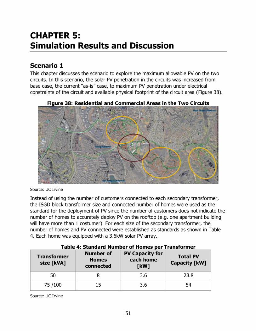
51
CHAPTER 5: Simulation Results and Discussion
Scenario 1 This chapter discusses the scenario to explore the maximum allowable PV on the two
circuits. In this scenario, the solar PV penetration in the circuits was increased from
base case, the current “as-is” case, to maximum PV penetration under electrical
constraints of the circuit and available physical footprint of the circuit area (Figure 38).
Figure 38: Residential and Commercial Areas in the Two Circuits
Source: UC Irvine
Instead of using the number of customers connected to each secondary transformer,
the ISGD block transformer size and connected number of homes were used as the
standard for the deployment of PV since the number of customers does not indicate the
number of homes to accurately deploy PV on the rooftop (e.g. one apartment building
will have more than 1 costumer). For each size of the secondary transformer, the
number of homes and PV connected were established as standards as shown in Table
4. Each home was equipped with a 3.6kW solar PV array.
Table 4: Standard Number of Homes per Transformer
Transformer
size [kVA]
Number of
Homes
connected
PV Capacity for
each home
[kW]
Total PV
Capacity [kW]
50 8 3.6 28.8
75 /100 15 3.6 54
Source: UC Irvine

52
For the commercial customers/buildings, the physical footprint of the rooftops was
estimated using “Google Earth View”, and the average solar panel measurements of 39
x 65 inch per 265 watts were used to determine the capacity that the available footprint
can host. Figure 39 shows the available rooftop spaces in one section of circuits.
Figure 39: Building Rooftop Footprint (One Section)
Source: Google Earth
With all the PV deployed on the circuit with the standardized number of homes, the
residential sector could host 8.697MW of PV and the commercial sector could host
2.66MW of PV. This resulted in a total of 11.36MW of solar PV on the entire circuit. This
was the capacity the circuits can host merely based on the available footprint and
rooftop spaces.
The system model previously developed was used to run simulations to determine if
any electrical constraints were violated with the deployment of maximum PV established
previously solely based on footprint. The simulation was conducted as a worst case
scenario where the PV production is at its highest and the load profile at its lowest. This
situation led to high gradients in the net load (similar to the famous duck curve) and
resulted in abnormal voltage on 13 phase C node points in the system. Figure 40 is a
plot of the voltage in a 24 hour period. While the voltage contraint is +/- 5% from the
nominal voltage, as can be seen in Figure 40, the voltage shot over +5% at peak PV
power generation. After such simulations, the PV capacity was adjusted at each of the
13 nodes (identified previously with volatege violations) and reduced by a total of
1.4MW PV capacity to avoid any violations. Figure 41 is a plot of the voltage at the
same node as Figure 40. It is shown that no voltage violations occurred with the new
PV capacity.

53
The results show that the maximum PV hosting capacity of the two circuits is 7.235MW
on residential housing and 2.66 MW on commercial buildings. Thus a total of 9.89MW of
solar PV can be installed on these circuits which leads to great gradients in the power
profile (duck curves) but is manageable since the voltage remained within the normal
voltage range on all the nodes. This is equivalent to 85.1% PV penetration (based on
maximum load on the circuits) on the two circuits given the maximum power at the
substation was 11.626MW.
Figure 40: Overvoltage at a Node with Max Photovoltaic Based on Footprint
Source: UC Irvine
Figure 41: Voltage at a Node with a New Adjusted Photovoltaic Penetration
Source: UC Irvine
54
Scenario 2 As previously discussed, battery energy storage was added as another DER to the
circuits having maximum PV penetration previously determined in order to assess the
impact of energy storage in scenarios with high PV penetration. The PV penetration is
increased to determine whether addition of energy storage helps increase the feasible
PV penetration on these circuits and ultimately the distribution system. The PV capacity
increased from 3.6 kW determined in the previous scenario without energy storage to a
maximum of 7kW per home which is consistent with data collected in California.
Although the U.S. average residential PV has been reported as 5.5kW6 in the state of
California 858 MW of residential solar PV was added in 2017 with an average size of 7
kW per residence7.
This scenario was divided into three groups, inspired by the ISGD project: 1) Residential
Energy Storage Unit (RESU), 2) Community Energy Storage (CES) and 3) Circuit
Battery. In this project, the data collected from the ISGD Project were utilized. The load
and PV profiles were extracted from the data set associated with a high load and high
PV day. May 15th, 2014 data of the ZNE block (9 homes), shown in Figure 42 were then
chosen for the simulations. The load in Figure 42 also includes the EV load. The EV
charge times were included according to the charge pattern determined from the ISGD
project. Out of the 9 homes in one block on average, 2 homes charge their EVs in the
morning, 1 home in the midday, 4 homes in the afternoon/evening and 2 homes at
midnight as shown in Figure 43.
6 “Solar Photovoltaic Technology,” Solar Energy Industries Association. [Online]. Available:
https://www.seia.org/research-resources/solar-photovoltaic-technology.
7 J. PYPER, “It’s Official. All New California Homes Must Incorporate Solar,” greentechmedia, 2018.
[Online]. Available: https://www.greentechmedia.com/articles/read/solar-mandate-all-new-california-
homes#gs.h2lwiSJC.

55
Figure 42: Block Load and Phovoltaic Profile – 5/15/2014
Source: UC Irvine
Figure 43: Average Electric Vehicle Charging Schedule per Home
Source: UC Irvine
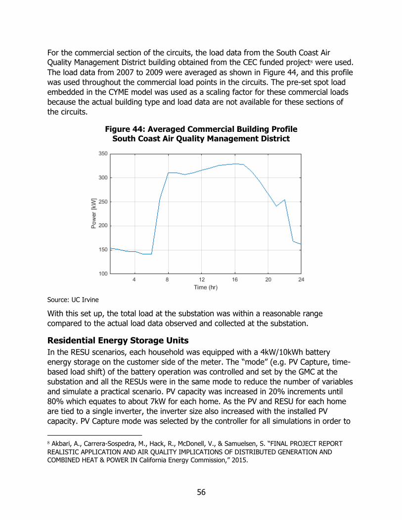
56
For the commercial section of the circuits, the load data from the South Coast Air
Quality Management District building obtained from the CEC funded project8 were used.
The load data from 2007 to 2009 were averaged as shown in Figure 44, and this profile
was used throughout the commercial load points in the circuits. The pre-set spot load
embedded in the CYME model was used as a scaling factor for these commercial loads
because the actual building type and load data are not available for these sections of
the circuits.
Figure 44: Averaged Commercial Building Profile South Coast Air Quality Management District
Source: UC Irvine
With this set up, the total load at the substation was within a reasonable range
compared to the actual load data observed and collected at the substation.
Residential Energy Storage Units
In the RESU scenarios, each household was equipped with a 4kW/10kWh battery
energy storage on the customer side of the meter. The “mode” (e.g. PV Capture, time-
based load shift) of the battery operation was controlled and set by the GMC at the
substation and all the RESUs were in the same mode to reduce the number of variables
and simulate a practical scenario. PV capacity was increased in 20% increments until
80% which equates to about 7kW for each home. As the PV and RESU for each home
are tied to a single inverter, the inverter size also increased with the installed PV
capacity. PV Capture mode was selected by the controller for all simulations in order to
8 Akbari, A., Carrera-Sospedra, M., Hack, R., McDonell, V., & Samuelsen, S. “FINAL PROJECT REPORT
REALISTIC APPLICATION AND AIR QUALITY IMPLICATIONS OF DISTRIBUTED GENERATION AND
COMBINED HEAT & POWER IN California Energy Commission,” 2015.

57
minimize grid import in order to reduce costs and maximize use of DERs. Figure 45
shows the total power profile at the substation, both circuits A and B, with different PV
capacities, and Figure 46and Figure 47 show the two circuits separately. In all three
figures, the “duck curve”9 can be identified which refers to the dip in the middle of the
day when PV production is at its highest and the steep ramping in the afternoon.
Figure 45: Total Power Profile at Substation
Source: UC Irvine
9 P. Denholm, M. O’Connell, G. Brinkman, and J. Jorgenson, “Overgeneration from Solar Energy in
California. A Field Guide to the Duck Chart,” November, 2015.

58
Figure 46: Circuit A Power Profile at Substation
Source: UC Irvine
Figure 47: Circuit B Power Profile at Substation
Source: UC Irvine
The two circuits consist of different building/load types as depicted in load profiles in
Figure 46 and Figure 47. Circuit A is mainly composed of residential loads with PVs and
RESUs, whereas Circuit B is mainly composed of commercial loads, with PV only on 10
buildings and no RESUs. For that reason, circuit A exports electricity to the grid during

59
the day as the PV capacities of the homes are increased to simulate and assess the
effects of the RESU in increasing renewable DER penetration. Circuit B shows a “dip” in
net load during the day as well, but it does not result in export to the grid since it does
not have a high penetration of DERs. Table 5 lists the results of the simulations which
shows that addition of RESUs increase the PV hosting capacity of the circuits. This table
also shows voltage violations at some nodes within the systems at 80% PV capacity
increase. For maximum PV, the PV capacity at the nodes with voltage violations were
reduced until there were no more violations. Voltage violations (>1.05p.u) at 5 nodes
close to the substation were also identified as shown in Figure 48. Voltage rise can be
caused by two factors, reverse power flow and decrease in line impedance. Due to the
over generation at peak PV production, as shown in Figure 49, it is expected that the
voltage rises beyond 1.05p.u. around the nodes closer to the substation, since the base
voltage is higher near the substation than the node points further away from the
substation. This is depicted in Figure 50and Figure 51, the voltage profiles presented for
the Scenario 1 PV and max case PV. In both figures, there are differences in the voltage
profiles for the closest and furthest nodes from the substation. The decrease in voltage
with the increase in distance from substation can be explained by voltage drop or line
drop, a phenomenon in circuits due to line current and line impedance.
Table 5: Result of Simulations – Residential Energy Storage Unit
PV Increase (%) Voltage Violations Total PV Capacity (MW)
0% (Scenario 1) None 9.89
20% None 11.342
40% None 10.129
60% None 12.789
80% Yes, 5 Nodes 15.683
Max None 15.29
Total Battery Capacity: 8.439MW/21.097MWh
Source: UC Irvine

60
Figure 48: Voltage Violation Node Location
Source: UC Irvine
Figure 49: Over Voltage at Node
Source: UC Irvine

61
Figure 50: Voltage Profile for Base Case Photovoltaic at Two Nodes
Source: UC Irvine
Figure 51: Voltage Profile for Max Photovoltaic Increase at Two Nodes
Source: UC Irvine
Community Energy Storage
In this scenario, each block (corresponding to each transformer) was equipped with a
25kW/50kWh battery energy storage (Community Energy Storage or CES). The
operation of these resources was controlled by the GMC. PV capacity was increased in
the same manner as the RESU scenarios. The initial conditions for the two CES modes
are shown in Table 6 and Table 7. The time intervals for Mode 1 were selected based

62
on the load stress at the transformer and the load limiting set points were selected in
order to reduce peak loads at the transformer node in order to relieve stress on the
infrastructure and assets. Similar to the RESU simulations, Mode 0, load limiting mode,
was selected by the controller during the simulations to minimize grid import and
reduce operation costs.
Table 6: Community Energy Storage Mode 1, Time based Permanent Load Shifting
Charging Time Interval Discharging Time Interval
1:00 ~ 4:00 17:00 ~ 22:00
Source: UC Irvine
Table 7: Community Energy Storage Mode 0, Load Limiting
Load Limit (kW) Generation Limit (kW)
5 0
Source: UC Irvine
Figure 52, Figure 53, and Figure 54 show the power profiles at the substation with
different PV capacities with CES, for Total, as well as circuit A, and circuit B separately.
Similar to the RESU scenarios, the net load at the substation resembles the famous
duck curve showing that addition of PV even with energy storage integration
exacerbates the duck curve. As previously mentioned, because most of the residential
housing is on circuit A, the impact of PV increase is more visible in Figure 53 associated
with circuit A compared to circuit B. Due to the difference in the battery capacity, circuit
A starts exporting electricity to the grid at 40% PV increase compared to 60% PV
increase associated with the RESU scenario.
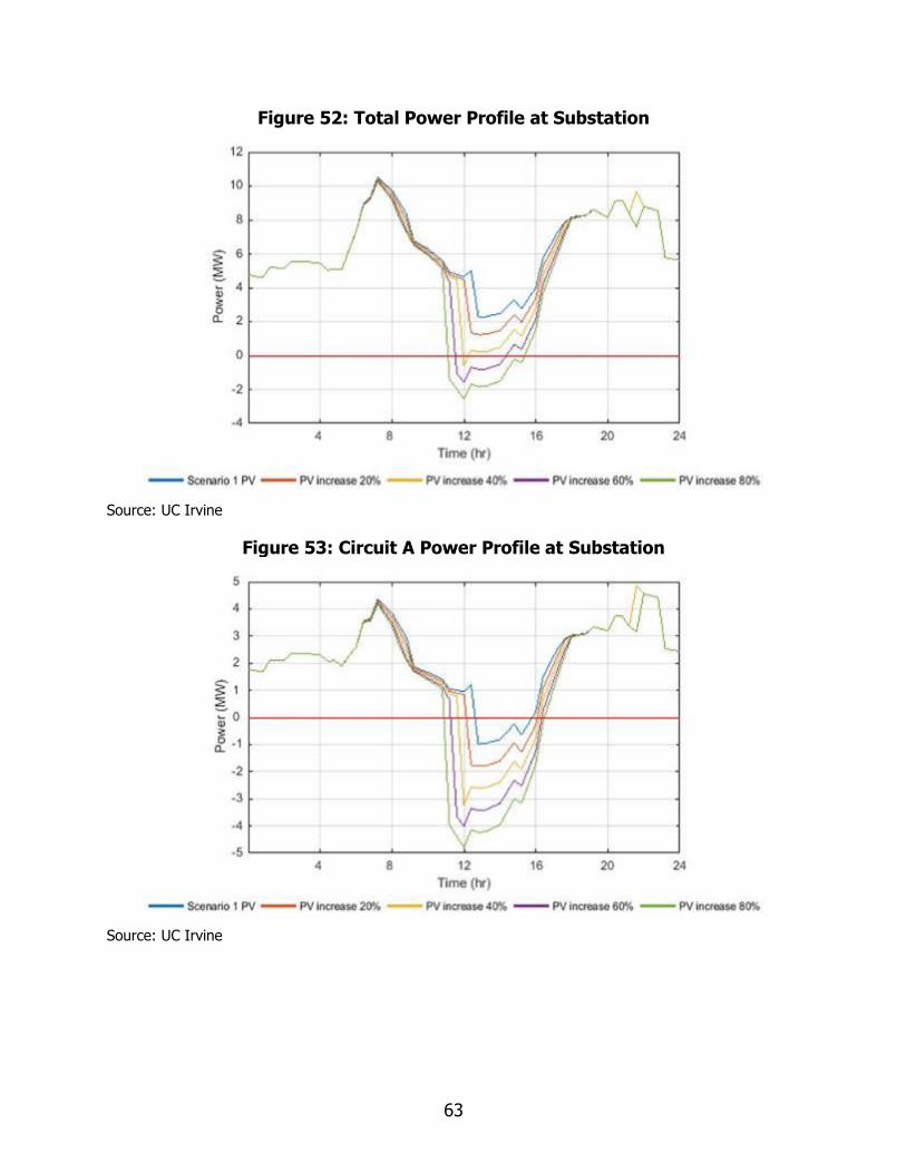
63
Figure 52: Total Power Profile at Substation
Source: UC Irvine
Figure 53: Circuit A Power Profile at Substation
Source: UC Irvine
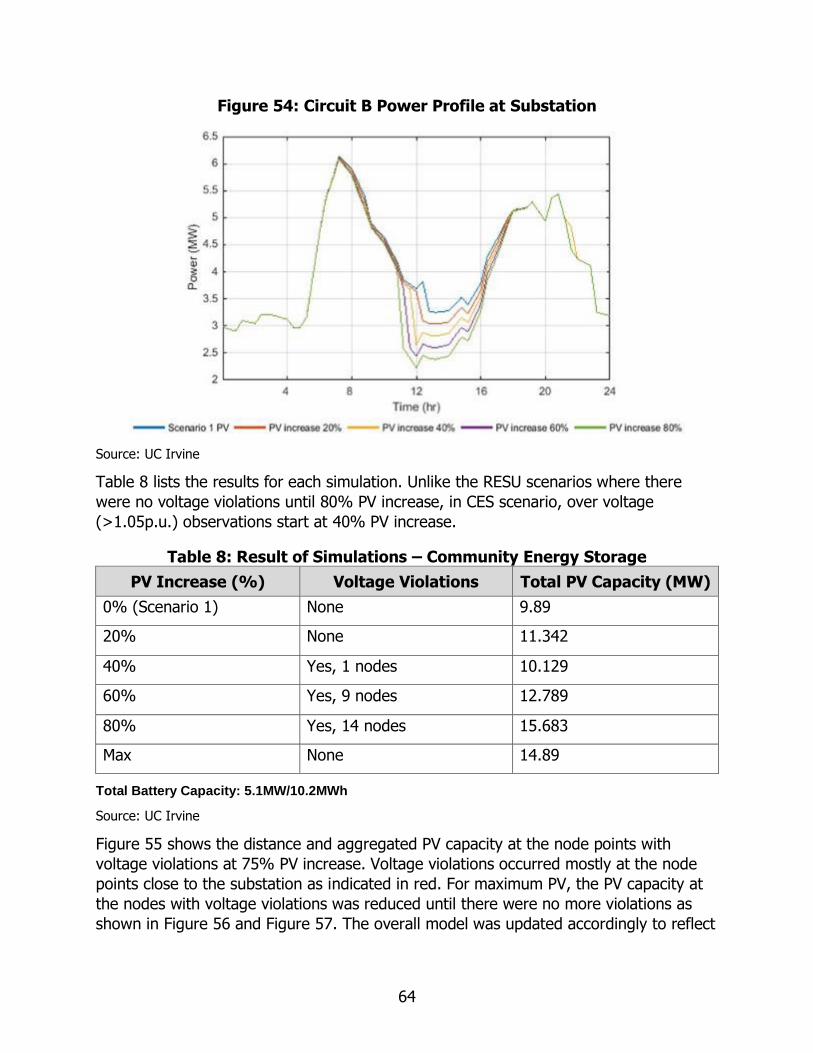
64
Figure 54: Circuit B Power Profile at Substation
Source: UC Irvine
Table 8 lists the results for each simulation. Unlike the RESU scenarios where there
were no voltage violations until 80% PV increase, in CES scenario, over voltage
(>1.05p.u.) observations start at 40% PV increase.
Table 8: Result of Simulations – Community Energy Storage
PV Increase (%) Voltage Violations Total PV Capacity (MW)
0% (Scenario 1) None 9.89
20% None 11.342
40% Yes, 1 nodes 10.129
60% Yes, 9 nodes 12.789
80% Yes, 14 nodes 15.683
Max None 14.89
Total Battery Capacity: 5.1MW/10.2MWh
Source: UC Irvine
Figure 55 shows the distance and aggregated PV capacity at the node points with
voltage violations at 75% PV increase. Voltage violations occurred mostly at the node
points close to the substation as indicated in red. For maximum PV, the PV capacity at
the nodes with voltage violations was reduced until there were no more violations as
shown in Figure 56 and Figure 57. The overall model was updated accordingly to reflect

65
these changes. Figure 58 shows the voltage profiles at the closest and furthest nodes
from the substation for maximum PV penetration.
The voltage violation node points near the substation were the same as the RESU
scenario, however, in the CES scenario, additional violation node points are present
near the end of the distribution circuit. Along with the closest node having the highest
voltage rise rate shown from section 0, this shows that the voltage rise rate was also
high with high penetrations at the end of the distribution line. This confirms the findings
from the ideal four bus model study included in the California Solar Initiative final
report10 performed by Advanced Power and Energy Program which studied the voltage
rise rate for high PV penetration at different locations in the distribution system:
beginning, middle and end, and concluded that high PV penetration fixed at the end
point of the distribution circuit results in the highest voltage rise rate. Therefore, high
voltage rises at node points near the substation and far node points of the substation
are as expected.
Figure 55: Voltage Violation Node Location
Source: UC Irvine
10 Final Report, “California Solar Initiative RD & D Program Process Evaluation,” 2017.
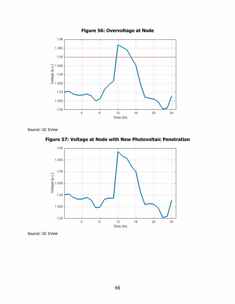
66
Figure 56: Overvoltage at Node
Source: UC Irvine
Figure 57: Voltage at Node with New Photovoltaic Penetration
Source: UC Irvine
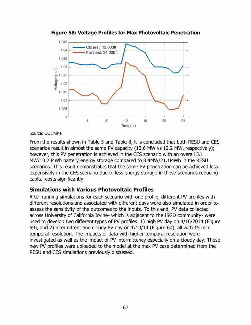
67
Figure 58: Voltage Profiles for Max Photovoltaic Penetration
Source: UC Irvine
From the results shown in Table 5 and Table 8, it is concluded that both RESU and CES
scenarios result in almost the same PV capacity (12.6 MW vs 12.2 MW, respectively);
however, this PV penetration is achieved in the CES scenario with an overall 5.1
MW/10.2 MWh battery energy storage compared to 8.4MW/21.1MWh in the RESU
scenarios. This result demonstrates that the same PV penetration can be achieved less
expensively in the CES scenario due to less energy storage in these scenarios reducing
capital costs significantly.
Simulations with Various Photovoltaic Profiles
After running simulations for each scenario with one profile, different PV profiles with
different resolutions and associated with different days were also simulated in order to
assess the sensitivity of the outcomes to the inputs. To this end, PV data collected
across University of California Irvine- which is adjacent to the ISGD community- were
used to develop two different types of PV profiles: 1) high PV day on 4/16/2014 (Figure
59), and 2) intermittent and cloudy PV day on 1/10/14 (Figure 60), all with 15 min
temporal resolution. The impacts of data with higher temporal resolution were
investigated as well as the impact of PV intermittency especially on a cloudy day. These
new PV profiles were uploaded to the model at the max PV case determined from the
RESU and CES simulations previously discussed.

68
Figure 59: Normalized University of California Irvine Photovoltaic Profile – High Photovoltaic Day (4/16/14)
Source: UC Irvine
Figure 60: Normalized University of California Irvine Photovoltaic–
Intermittent Photovoltaic PV Day (1/10/14)
Source: UC Irvine

69
The results of the simulations for the RESU and CES cases were similar. Figure 61 to
Figure 64 show the power profiles at the substation for various PV profiles studied.
Figure 61: Power Profile with High University of California Irvine Photovoltaic Profile – Residential Energy Storage Unit
Source: UC Irvine
Figure 62: Profile with Intermittent University of California Irvine
Photovoltaic Profile – Residential Energy Storage Unit
Source: UC Irvine

70
Figure 63: Power Profile with High University of California Irvine Photovoltaic Profile – Community Energy Storage
Source: UC Irvine
Figure 64: Power Profile with Intermittent University of California Irvine
Photovoltaic Profile – Community Energy Storage
Source: UC Irvine

71
After running all four simulations, 4 nodes from the CES scenario and 9 nodes from the
RESU scenarios experience over voltages at high PV penetrations. These nodes are the
same nodes seen for the previous CES scenarios from section 0 with ISGD PV profile
data.
Renewable Penetration
In order to determine the renewable penetration (based on energy), the averaged load
and PV data are used for one whole year of the ZNE block (Figure 65). The overall
power seen at the substation, was comparable to the actual substation power data
recorded during the ISGD project.
Figure 65: Annual Average Load and Photovoltaic Profile
Source: UC Irvine
The 𝑅𝑒𝑛𝑒𝑤𝑎𝑏𝑙𝑒 𝑃𝑒𝑛𝑒𝑡𝑟𝑎𝑡𝑖𝑜𝑛𝑇𝑜𝑡𝑎𝑙 is 39% (associated with 15.29 MW of PV) when all the
PV generated electricity was used and not curtailed, equation 5.1. However, the two
circuits are not able to consume all the PV generated electricity and exported to the grid
as shown in
Figure 45 and Figure 52. Exporting can be limited due to the interconnection
agreements, and as the exporting hours coincide with the belly of the “duck curve,” it is
likely that the grid is unfavorable of such export, resulting in negative prices or
curtailment.
𝑅𝑒𝑛𝑒𝑤𝑎𝑏𝑙𝑒 𝑃𝑒𝑛𝑒𝑡𝑟𝑎𝑡𝑖𝑜𝑛𝑇𝑜𝑡𝑎𝑙 = Total Annual PV Generation
Total Annual Load (6.1)
To determine the renewable penetration solely for the two circuits, taking into account
the curtailment, the below equation was used.

72
𝑅𝑒𝑛𝑒𝑤𝑎𝑏𝑙𝑒 𝑃𝑒𝑛𝑒𝑡𝑟𝑎𝑡𝑖𝑜𝑛𝑆𝑢𝑏𝑠𝑡𝑎𝑡𝑖𝑜𝑛 = Total PV Generation − Curtailed Energy
Total Load (6.2)
As shown in Table 9, the no storage case has over a 6.4 MWh of curtailed energy and
the renewable penetration is 35.8%. By adding energy storage, the renewable
penetration increases to 37.5% for the RESU case and 35.3% for the CES case. For
both cases, there was only a slight difference in the maximum total PV capacity which
resulted in small renewable penetration difference.
Table 9: Renewable Penetration
Scenario Total PV Capacity
(MW)
PV Energy for 1 day (MWh)
Curtailed Energy (MWh)
Load for 1 day
(MWh)
Renewable Penetration
(%)
No Storage 15.29
(RESU) 81.1 6.4 208.1 35.8
No Storage 14.89 (CES)
78.0 4.7 208.1 35.2
All RESU 15.29 81.1 3.1 208.1 37.5
All CES 14.89 78.0 4.2 208.1 35.4
Source: UC Irvine
Circuit Battery
A 2MW/500kWh battery energy storage was simulated at the substation, referred to as
the “circuit battery” since it served the entirety of the two circuits. During the
simulation, the controller set the mode of the circuit battery to mode 0, load limiting
mode, in order to minimize grid import at the substation and maximize the use of DERs
and reduce costs. The parameters were set as Table 10.
Table 10: Circuit Battery Parameters – Mode 0
Parameter Value
Initial SoC 50%
Efficiency 96%
Load Limit 9 MW
Generation Limit 0 MW
Source: UC Irvine

73
Figure 66 shows the power profile at the substation without and without the circuit
battery. Given the low energy capacity of the battery, there are minor impacts on the
two circuits.
Figure 66: Circuit Battery Impact on Power Profile
Source: UC Irvine
To further assess the impact of a larger battery energy storage, a series of different
sized batteries were simulated with a new load limiting set point of 7MW. As shown in
Figure 67, 2MW battery energy storage with 2, 4, 6 MWh capacities were simulated.
With the 2MW/6MWh battery, nearly zero export of electric was possible at the
substation by charging the battery using all excess solar generated electricity and
discharging to shave the peak loads. This can help alleviate the duck curve issues in the
overall grid.

74
Figure 67: Circuit Battery Impact on Substation – 2MW Battery
Source: UC Irvine
Scenario 3 For this scenario, all homes were assumed to be equipped with smart appliances and
energy management system capable of responding to DR requests. DR signals were
sent to homes from the controller to resolve any system violations that occur in the
system. Simulations with different DR load shed percentage, and different participation
rate were conducted. The DR signal was sent from the grid operator from 5PM to 9PM.
This time block is the super peak block from the CAISO Proposed TOU Periods11 and
reflects the high peak load and steep ramp up curve resulting from PV generation (the
duck curve). The simulation was done on both maximum scenarios of CES and RESUs
from the previous section. DR signals were sent to reduce 20% and 40% of the total
load consumed from each home. Also for each corresponding percentage and signal,
different participation percentage was simulated. After looking at the ISGD data for
homes, it was reasonable to reduce up to 40% of the home load which is equivalent to
turning off 75% of the lights and reducing the air conditioning load to half (or other
combinations). For EVSEs, a DR signal of 50% reduction in charge rate was sent. Figure
68 shows the maximum CES case with 20% DR and Figure 69 shows the same case
with 40% DR. It is observed that only a small difference in the load reduction occurred
between 50% and 100% participation. This was due to the fact that all the homes
which had the EV charging during those hours participated to reduce 50% of the EV
charge capacity, and the other non-participating homes did not have EV charging
11 “CAISO time-of-use periods analysis,” 2016.

75
scheduled during this time. This shows that DR on EV charging, which is a large load
compared to other residential loads, has a large impact on reducing load.
Figure 68: 20 Percent Demand Response Results
Source: UC Irvine
Figure 69: 40 Percent Demand Response Results
Source: UC Irvine

76
Figure 70: Net Load at Substation With and Without Demand Response
Source: UC Irvine
These results show that using DR can help relieve the ramping requirements in the
duck curve in the afternoon by reducing demand during these intervals as shown in
Figure 70.
Scenario 4 In the circuit independent scenarios, the circuit was equipped with a 2MW/500kWh
circuit battery and a 2.8MW PAFC at the substation with the given parameters in Table
11. The current substation does not have the required footprint to host a fuel cell of
this size and a battery. However, this scenario was simulated and investigated to study
the possible impacts of a fuel cell at a substation on reliability and outage reduction12.
Table 11: Fuel Cell Parameters13
Capacity
[kW]
Ramp Up Rate [kW/s]
Ramp Down Rate [kW/s]
Base Load
[%]
400 10 -20 56
Source: UC Irvine
12 B. Shaffer, B. Tarroja, and S. Samuelsen, “Dispatch of fuel cells as transmission integrated grid energy
resources to support renewables and reduce emissions,” Appl. Energy, vol. 148, no. x, pp. 178–186, 2015.
13 Clear Edge Power, “Electric Load - Following Capability of the PureCell ® Model 400 Fuel Cell System,”
no. January, 2013.
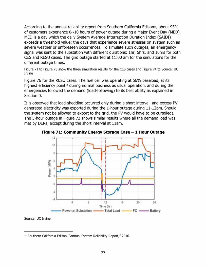
77
According to the annual reliability report from Southern California Edison14, about 95%
of customers experience 0~10 hours of power outage during a Major Event Day (MED).
MED is a day which the daily System Average Interruption Duration Index (SAIDI)
exceeds a threshold value; the days that experience severe stresses on system such as
severe weather or unforeseen occurrences. To simulate such outages, an emergency
signal was sent to the substation with different durations: 1hr, 5hrs, and 10hrs for both
CES and RESU cases. The grid outage started at 11:00 am for the simulations for the
different outage times.
Figure 71 to Figure 73 show the three simulation results for the CES cases and Figure 74 to Source: UC Irvine
Figure 76 for the RESU cases. The fuel cell was operating at 56% baseload, at its
highest efficiency point13 during normal business as usual operation, and during the
emergencies followed the demand (load-following) to its best ability as explained in
Section 0.
It is observed that load-shedding occurred only during a short interval, and excess PV
generated electricity was exported during the 1-hour outage during 11-12pm. Should
the system not be allowed to export to the grid, the PV would have to be curtailed).
The 5-hour outage in Figure 72 shows similar results where all the demand load was
met by DERs, except during the short interval at 11am.
Figure 71: Community Energy Storage Case – 1 Hour Outage
Source: UC Irvine
14 Southern California Edison, “Annual System Reliability Report,” 2016.

78
Figure 72: Community Energy Storage Case – 5 Hour Outage
Source: UC Irvine
During the 10 hour outage which goes on until the evening, significant load-shedding
was required after 4pm to ensure supply/demand balance and system stability. About
70% of the load was dropped in order to match the local electricity generation and the
demand load. While dropping this much of the electricity demand seems excessive; the
alternative is for the system to experience a complete outage and lose critical loads.
Figure 73: CES Case – 10 Hr Outage
Source: UC Irvine

79
For the RESU cases, the overall results are similar; however, due to the difference in
operation and size of energy storage units, significant load shedding was required from
11am to 12pm as shown in Figure 74.
Figure 74: RESU Case – 1 Hr Outage
Source: UC Irvine
Both the 5 hour and 10 hour outage simulations, depicted in Figure 75 and Source: UC Irvine
Figure 76 respectively, are similar to the CES cases requiring significant load-shedding
during the evening hours when there is no PV generation and only the fuel cell and
energy storage units are available for electricity generation.

80
Figure 75: RESU Case – 5 Hr Outage
Source: UC Irvine
Figure 76: RESU Case – 10 Hr Outage
Source: UC Irvine
For a 24-hour emergency zero import situation, an emergency signal was sent to the
substation and the controller switched the modes of the DERs in the circuit to
accommodate the grid outage as described in Section 0 and Figure 36.
During the CES scenario simulation, the two circuits were kept “live” with heavy load
shedding for periods of high loads and zero PV. Zero load was dropped and excess PV

81
generated electricity was available during high solar hours but up to 70% load shedding
was required during the evening. Figure 77 shows the 24 hour power profiles for the
two circuits.
Figure 77: CES 24 Hour Power Outage Profile
Source: UC Irvine
For the RESU scenario, the grid was also “live” during the 24hour outage. As the
controller sends each home the demand response based on the total load, the total
output load is harder to manage because each home’s net load depends on the battery
storage dispatch associated with that home. With the current model, the total load was
managed as depicted in Figure 78. The figure shows spikes of power export due to the
mismatch of the fuel cell ramp down rate and immediate load drop from DR.

82
Figure 78: RESU 24 Hour Power Outage Profile
Source: UC Irvine

83
CHAPTER 6: Task 5: Retail/Distribution Market
Electricity Markets and Market Participation for Distributed Energy Resources
The generation, transmission, distribution, and sale of electrical energy has been
undergoing a major transformation. Driven by the promise of lower prices from
competition, the traditional regulated monopoly, vertically integrated utility is being
disaggregated into a system of competitive markets. This transformation has been
taking place in three main arenas:
1. Wholesale Markets and Transmission
2. Retail Markets
3. Distribution
Wholesale Markets involve the sale of bulk energy (MWH) and capacity (MW) between
large generators and retail Load Serving Entities (and sometimes large industrial
customers). The construction and ownership of transmission lines has also been opened
to competition. This has been the first and most common area for transition to a market
structure. About 2/3 of US customers now receive power from wholesale markets and
about 1/3 from vertically integrated regulated monopolies. While the transmission
systems themselves are still mostly owned by the utilities that built them, who are
referred to as Transmission Owners (TO), the transmission system and the
energy/capacity markets are operated by an independent entity called either an
Independent System Operator (ISO) or Regional Transmission Organization (RTO).
Retail Markets in many states allow customers to choose their retail Energy Services
Provider (ESP) which in turn purchases energy on the wholesale market. Where this
function has been separated from the regulated utility, the entity retaining ownership
and operation of the physical distribution “wires” system is called the Utility Distribution
Company (UDC) or Distribution Owner (DO). Metering and billing can also be separated
or retained by either the ESP or UDC. If a customer does not pick an alternative ESP,
the UDC fills this role as a default Provider of Last Resort (POLR) also known as
Standard Offer Service (SOS) or “bundled service.” Retail markets are available in
thirteen states and the District of Columbia. They also exist in the UK and some other
foreign countries. Retail choice is most used by industrial customers, then by
commercial customers, and least (often none) by residential customers. This makes
sense since larger consumers have more bargaining power and regulators often
artificially keep rates down for residential customers (voters). Benefits to consumers
have been marginal or unclear, in general.

84
A more recent trend has been to try and create a Distribution Market to increase the
opportunity for DERs including generation, storage or demand response, to sell to other
parties. Three subcategories of distribution markets are:
1. Value of DER Markets, where DER sells services to the UDC in lieu of traditional
wires solutions,
2. Aggregator Role, where the Distribution System Operator (DSO) to aggregate
DER output and sell it into the wholesale market, and
3. Direct Access, where DER can sell to any customer over the distribution system.
As in transmission, the physical distribution system is owned by the UDC/DO
which is a regulated monopoly utility. The DSO would have to operate a market
and oversee distribution planning to ensure transparency and fairness. Whether
the UDC/DO can perform these DSO functions with regulatory oversight or
whether an independent DSO (IDSO) similar to the ISO/RTO model is up for
debate.
DER Wholesale Market Participation Benefits (Existing Opportunities) If a resource is connected to the transmission system, it can connect to CAISO grid (see
Appendix B for details) and go through new resource implementation and participate in
CAISO markets that it qualifies for via a scheduling coordinator.
For resources that are in the distribution system (and sub-transmission system), CAISO
accepts bids for Energy and Ancillary Services from Distributed Energy Resource
Aggregations only if they are represented by a Distributed Energy Resource Provides
(DERP) which has entered into a Distributed Energy Resource Provider Agreement with
the CAISO to comply with all applicable provisions of the CAISO Tariff. A Distributed
Energy Resource Aggregation consists of 1 or more DERs and it need to be at least 0.5
MW, and it must be located in a single Sub-LAP (Load Aggregation Point). A map of the
sub-LAPs is shown in Figure 79. If DERs are located at different P-Nodes, the
Distributed Energy Resource Aggregation needs to be smaller than 20 MW. Each
Distributed Energy Resource should then provide a net response at P-Node (or P-
Nodes) in a single Sub-LAP consistent with CAISO dispatch instructions. Note that a
DER participating in a Distributed Energy Resource Aggregation cannot participate in a
retail net metering program or participate in CAISO markets separate. Thus, both net-
metering and wholesale market participation cannot be counted simultaneously towards
the benefits of DERs.
In order to access the P-Nodes, transmission system and ultimately CAISO markets,
DERs need to use the distribution system and the infrastructure owned by the utility
and thus they require to have a WDAT(details included in Appendix B). DERs must be
directly metered with a meter complaint with the utility company for the purpose of
settlement. However, if the DER aggregation is larger than 10MW or it provides

85
ancillary services, the information should be provided to the CAISO EMS through
telemetry complying with CAISO standards for direct telemetry. In summary, for DERs
to participate in CAISO wholesale markets, they need to have a WDAT with the utility
and be part of a Distributed Energy Resource Aggregation represented by a DERP and
the bids need to be submitted by a scheduling coordinated. Details of requirements and
responsibilities of DERPs, Distributed Energy Resource Aggregations, and other entities
can be found in CAISO Tariff15.
Figure 79: CAISO Sub-LAP Map
Source: California Independent System Operator, Proxy Demand Resource (PDR) &Reliability Demand Response Resource (RDRR) Participation Overview.
https://www.caiso.com/Documents/PDR_RDRRParticipationOverviewPresentation.pdf
15 California Independent System Operator. California Independent System Operator Corporation Fifth
Replacement FERC Electric Tariff. November 2018. http://www.caiso.com/Documents/ConformedTariff-asof-
Nov15-2018.pdf

86
There are several CAISO products available for Distributed Energy Resource
Aggregation that include not only distributed generation but also energy storage and
controllable loads. One of these products is Non-Generating Resources or NGRs. NGRs
can provide all services. (Note that CAISO has another resource model for storage,
Pump Storage, as well which does not apply to the discussions in this section).
Others product available are Proxy Demand Resource (PDR) and Reliability Demand
Response Resource (RDRR). PDG can provide Energy, Non-Spinning Reserve, and
Residual Unit Commitment (RUC), while RDRR can provide only Energy. Note that these
two products are both similar to demand response and thus reduce/curtail demand and
thus do not inject any power into the system and thus will not require a WDAT with the
utility. PDRs can bit into day-ahead energy market, day-ahead and real-time non-
spinning reserve market and 5-minute real-time energy market and must have a
minimum load curtailment of 100kW for energy market and 500MW for non-spinning
reserve, and smaller loads can be aggregated to meet the minimum.
RDRR can submit bids to day-ahead energy market but cannot submit ancillary services
bids and must respond to a reliability event, RDRR should have a minimum load
curtailment of 500kW and deliver reliability energy in real-time reaching full curtailment
within 40 minutes and should be able to run a minimum of 1 hour and maximum of 4.
DERs have several benefits including reduced costs, avoided transmission and
distribution losses, reduced emissions and reduced RPS procurements which have been
discussed in several previous studies.16 17 18 Participating in electricity market, can further
increase the benefit to cost ratio of DERs making them more attractive to investors and
ultimately help increase their penetration which will have societal benefits in terms of
reduced emissions and higher reliability. To demonstrate this, a 2MW/4MWh battery
energy storage previously used as the circuit battery is simulated at the distribution
system and its benefit to cost ratio of the battery was determined including participation
in wholesale market using EPRI StorageVet.19 This analysis takes into account all PV
production and all the loads in the two circuits and the battery is operated in a manner
to optimize the benefits during the project lifetime. The cost/benefit results are shown
in Figure 80. The costs include capital costs, replacements costs, and O&M costs. Note
that for this analysis it is assumed that the battery is controlled by the utility and the
16 Razeghi, G., Gu, F., Neal, R., Samuelsen, S. A generic microgrid controller: concept, testing, and
insights. Applied Energy. 2018; 229:660-671.
17 Li, M., Zhang, X., Li, G., Jiang, C. A feasibility study of microgrids for reducing energy use and GHG
emissions in an industrial application. Applied Energy. 2016;176:138-48.
18 Conti, S., Nicolosi, R., Rizzo, SA, Zeineldin, HH. Optimal Dispatching of Distributed Generators and
Storage Systems for MV Islanded Microgrids. IEEE Transactions on Power Delivery. 2012;27:1243-51
19 Electric Power Research Institute. https://www.storagevet.com/

87
customer load and PV profile are that of the total of the two circuits. This approach
treats the two circuits as one single entity (similar to a microgrid). As it can be
concluded from Figure 80, market participation (including day-ahead and real-time
energy, various ancillary services such as non-spinning reserve and frequency
regulation, and resource adequacy) increases the benefits of the circuit battery
considerably.
The hourly operation of the circuit battery resulting in cost/benefit shown in Figure 80,
for the first seven day of August is shown in Figure 81. Each plot represents one day.
Operation for the entire month of August is shown in Figure 82.
Figure 80: Cost/Benefit Analysis for the Circuit Battery (2MW/4MWh)
Source: UC Irvine

88
Figure 81: Circuit Battery Operation for the First Week of August
Source: UC Irvine
Figure 82: Circuit Battery Operation for the Month of August
Source: UC Irvine
Note that the benefit of market participation needs to be analyzed for each DER and
depends on the type and characteristics of the DER, customer load and other
generation/DER behind the meter, and location of the DER (in terms of LMP, and utility
rates and available programs). For example, the analysis was repeated for several ZNE
homes, using the home demand and solar generation. Constraints used are similar to
those used in the simulation of the circuit, with the roundtrip efficiency set as 96% and
state of charge (SOC) limited between 20% and 90%. It is further assumed that the
system is owned and controlled by the customer, and the battery (4kw/10kWh RESU)
participates in SGIP (Self-Generation Incentive Program), and SCE demand response

89
programs. SCE TOU tariffs and rates20 are used for this analysis. The cost/benefit results
for one of these homes is shown in Figure 83 . As it can be seen from this figure, the
majority of the RESU benefits is associated with shifting load and providing demand
response as well as frequency regulation. However other markets such as spinning and
non-spinning reserve provide small and insignificant financial benefits to the RESU. This
result is different from the circuit battery for which the market participation proved
more beneficial compared to demand response and retail load-shifting. These results
demonstrate that the benefits of market participation and various program for the DERs
depend on size, characteristics and location of the DER. The results associated with
other homes, using their load and PV profiles are similar as well.
The hourly operation of the RESU, associated with home #1 in ZNE block for 31 days of
August is shown in Figure 84.
Figure 83: Cost/Benefit Analysis Associate with a RESU (ZNE Home 1)
Source: UC Irvine
20 Southern California Edison. Schedule TOU-D, Time of Use, Domestic. https://www1.sce.com/NR/sc3/tm2/pdf/ce360.pdf

90
Figure 84: Battery Operation for the Month of August (ZNE Home 1)
Source: UC Irvine
Cost/benefit analysis was repeated for another case in which the operation of the
battery energy storage is controlled by the utility (instead of customer). In this case,
there is a slight reduction in benefits of load-shifting but the rest are almost identical
showing that for a small behind the meter battery energy storage, whether or not its
operation is controlled by the utility has little impact on the benefit to cost ratio of the
system.
From the analysis and results shown in this section, it can be concluded that market
participation can be beneficial to the DERs and increase their benefit to cost ratio.
However, the extent and significance of these benefits depend on location of the DERs,
size and characteristics of the resource and available programs.
Possible Future Opportunities: Distribution/Retail Markets So far in this chapter, a brief discussion of DER interconnection and tariffs were
provided along with benefits of wholesale market participation for the DERs used in this
project such as the RESU and circuit battery. Wholesale market participation contributes
to and is in response to system (overall grid) needs which at times might not align with
local needs of the distribution system. Furthermore, process of qualifying for CAISO
market participation is complicated, time-consuming and has financial risks associated
with it. As the penetration of DERs increases, the grid will experience a paradigm shift
from a more centralized generation to distributed generation in which load and
generation are located close to one another and some generation resources are owned
by the customer and located behind the meter. Figure 85 shows the future smart grid
including both centralized and distributed generation as well as microgrids and
advanced technologies.

91
With increased DER penetration, ISO requires more distribution grid real-time visibility,
forecasting of DER impacts at the transmission interface, and coordination between the
ISO, utility, and DER aggregators in order to ensure a reliable and economic grid. With
this added complexity, there has been renewed interest in distribution markets and
concept of Distribution System Operator or DSO, comparable to ISO or TSO but
responsible for the distribution system and serving the local needs.
Figure 85: Future Smart Grid
Source: UC Irvine
To facilitate participation of DERs in the market, one option is to basically expand the
ISO to include the distribution system and its resources. Note that currently the DERPs
provide a net response at a P-Node and CAISO does not optimize or take into account
the individual operation of DERs. To this end, ISO needs to add a full network model of
the distribution system and include all the DERs in the centrally optimized ISO markets.
DSO (which can be the utility) in the case act as the entity responsible for reliability of
the distribution system as well as coordinating the reliability at the transmission-

92
distribution (T-D) interface. This approach has been referred to as “Minimal DSO”21 22 23.
In addition to requiring a complete model of the distribution system, this approach
requires real-time monitoring of all DERs by the ISO, as well as communication and
telemetry. This approach is shown in Figure 86. As it is shown in this figure, as the
number of DERs increases, the operation and central optimization of ISO becomes
increasingly more complicated and the network and distribution models needs to be
updated, thus making this approach very complicated and not suitable for scaling to
cover the entire ISO territory not be mention the computational power required to solve
a mixed-integer non-linear optimization with this many variables.
Figure 86: Option 1: ISO Managing DERs (Minimal DSO)
Source: UC Irvine
Another option is to set up a market in the distribution system which is similar to the
ISO wholesale market. This market will be run and operated by the DSO and DERs will
have the option to participate in this market. In addition to T-D interface reliability,
energy (or other services and products) transaction at the T-D interface will be the
responsibility of the DSO as well as scheduling and dispatch of resources in the
21 De Martini, P., Kristov, L. Distribution systems in a high distributed energy resources future. 2015.
https://emp.lbl.gov/sites/all/files/lbnl-1003797.pdf
22 De Martini, P., Kristov, L. 21st Century Electric Distribution System Operations. 2014. http://resnick.caltech.edu/docs/21st.pdf
23 Kristov, L. Policy, Technology and Architecture for a 21st Century Electric System. 2017

93
distribution system. This approach also known as Total or Full DSO is shown in Figure
87. In this approach the only information crossing the T-D interface is the net load (+
or 1) and the marginal price of the distribution market (or the market clearing price
associated with each DSO). This considerably reduces the number of variables in the
ISO central optimization and result in:
• Reduced complexity
• Balancing supply and demand locally
• Serving local needs of higher reliability and increased renewable penetration
• Scalability
• Possible active and direct participation of demand (see section 0)
• Facilitating participation of microgrids and DERs (without the need for
aggregation and distributed energy resources providers)
Figure 87: Option 2: Distribution Market (Total or Full DSO)
Source: UC Irvine
The objective of the DSO optimization will be to minimize the overall system cost similar
to the ISO; however, this system is limited to the distribution system under DSO
authority. This optimization is constraint also to ensure the reliability of the distribution
system as well as T-D interface. This cost includes the cost associated with the DERs
inside the territory of the DSO (includes production cost, and start-up cost depending
on the technology), and the cost associated with import/export from/to other DSOs and
the ISO. The general objective function is shown in Eq(7.1). In this equation, the first
part is associated with the DER generation cost in which Ng is the total number of DERs,

94
Ci is the cost function of i-th DER, and S(i,t) is the start-up cost of this unit at time t while P(i,t) is how much this DER is generating (or consuming in case of storage). The
second term in Eq(7.1) is associated with transactions with other DSOs. NDSO is the
number of DSOs that do transaction with the DSO under study, TPDSO(j,t) is the
transaction price with j-th DSO at time t and ImpDSO(j,t) is the amount of import (or
export) with the j-th DSO. The last term in Eq(7.1) is associated with transaction with
the ISO. The price of energy transactions between this DSO and the ISO is set as the
locational marginal pricing (LMP(t)) at a P-Node corresponding to the DSO, and ImpISO(t) represents the amount of import (or export) with at the T-D interface.
Minimize
{∑[𝐶𝑖 𝑃(𝑖, 𝑡) + 𝑆(𝑖, 𝑡)]
𝑁𝑔
𝑖=1
} + { ∑ [𝑇𝑃𝐷𝑆𝑂(𝑗, 𝑡) 𝐼𝑚𝑝𝐷𝑆𝑂(𝑗, 𝑡)]
𝑁𝐷𝑆𝑂
𝑗=1
} + 𝐿𝑀𝑃(𝑡)𝐼𝑚𝑝𝐼𝑆𝑂(𝑡) (7.1)
The optimization is subject to several constraints. The first and most obvious constraint
is balance of supply and demand shown in Eq(7.2). In this equation D(t) represents
demand within the DSO at time t.
𝐷(𝑡) = {∑ 𝑃(𝑖, 𝑡)
𝑁𝑔
𝑖=1
} + { ∑ 𝐼𝑚𝑝𝐷𝑆𝑂(𝑗, 𝑡)
𝑁𝐷𝑆𝑂
𝑗=1
} + 𝐼𝑚𝑝𝐼𝑆𝑂(𝑡) (7.2)
Several constraints are associated with physical limits of the resources. These include
generation limits (charge/discharge limit for energy storage), ramping up and down
limits, SOC limits, and thermal unit minimum start-up time and minimum down times.
Other constraints such as minimum on/off times are economic constraints. Another
group of constraints are used to ensure the required ancillary services are available.
These constrains associated with energy storage were previously discussed and are
detailed in several previous publications24 25 26.
24 Razeghi, G., Brouwer, J., & Samuelsen, S. A spatially and temporally resolved model of the electricity
grid – Economic vs environmental dispatch. Applied Energy 2016; 178, 540–556.
25 Razeghi, G. The Development and Evaluation of a Highly-Resolved California Electricity Market Model to
Characterize the Temporal and Spatial Grid, Environmental, and Economic Impacts of Electric Vehicles. Ph.D. Dissertation. University of California, Irvine. 2013
26 Razeghi, G., & Samuelsen, S. Impacts of plug-in electric vehicles in a balancing area. Applied
Energy.2016; 183, 1142–1156

95
Depending on the location of the DSO, there might be limit associated with specific
pollutants and emissions. This constraint is shown in Eq(7.3). In this equation, EM(i.j) is the emission factor for pollutant j of unit i, and SE(i,j,t) is the start-up emission of unit i. REL(j) is a specific region’s limit for the same pollutant.
∑ ∑[𝐸𝑀(𝑖, 𝑗)(𝑃(𝑖, 𝑡)) + 𝑆𝐸(𝑖, 𝑗, 𝑡)] ≤ 𝑅𝐸𝐿(𝑗)
𝑁𝑡
𝑡=1
𝑁𝑔
𝑖∈𝐴
(7.2)
Other constraints are associated with the electrical system such as the possible
restriction at the T-D interface. Since the current system is designed based on central
generation, it is expected that all the distribution load can be served by the ISO;
however, if the upgrades to the transmission system in the future take into account the
increasing DER penetration, there will be a limit at the T-D interface.
Overall this problem is a non-linear problem and taking the unit commitment approach,
it is a mixed-integer non-linear problem which is difficult to solve. Moreover, for the
current project, since the size of the DSO encompassing the two circuits is much
smaller than the ISO territory, it is expected that the operation of the DSO in general
will not have significant impact on the result of the ISO market (the LMP variable shown
in Eq(7.1). However, as the number of DERs and DSOs grow, the ISO market prices
and LMP will be affected by the operation of the DSOs and as a result LMP in Eq(7.1) is
not known anymore and becomes a variable itself. This means that the ISO
optimization and DSO optimization will be coupled and even more complicated to solve.
In the next section, a simple approach is taken for the DSO in which the ISO prices are
considered known, solar PV (and other renewables) are considered must-take resources
in the market, and the behavior and benefits of the DSO market for the retail customer
are assessed.
Participation of Retail Customers (Retail Market)
The focus of the distribution market so far has been on the resources and their
providing services through the DSO market. The buyer in this market can be utilities,
entities representing a group of customers, or retail customers. Direct participation of
retail customers is referred to as retail market. Several states already allow customers
to choose the entity they want to buy electricity from and that entity (ESP) interacts
directly with the wholesale market, and they pay a fee to use the infrastructure (to the
utility or distribution owner). Distribution markets provide another option for the
customers and that is their direct participation in the market. Benefits of community
choice aggregation include increased local control over rates, possible savings for the
customer, and possible increase in DER and renewable penetration. However, so far
benefits to the customer have been marginal and unclear and EIA (Energy Information
Administration) reports that electricity residential retail choice participation has declined
since 2014 peak (from 17.2 million customers in 2014 to 16.2 million customers in

96
2016)27 28. While the benefits to the customers are in doubt, it is widely believed that
participation of retail customers in the market will result in flexibility of the demand
side. This is anticipated because of the fact that the wholesale prices or distribution
market prices will flow down to the retail customer and thus the customer will have
visibility in the real-time prices which encourages the customer to high prices by
reducing demand and overall increase the flexibility of the electricity demand. To assess
this, a RESU home previously described and used in this project, is assumed to be
directly involved with the market. The average market prices for the CAISO in 2017 are
used for this purpose and the values are normalized in order to get an average daily
price profile29. This price profile is shown in Figure 88a. It is assumed that for prices
higher than 0.7., the customer tries to reduce its demand by first discharging the
battery and second do demand response (with a maximum of 40%) if necessary to
reduce its demand as much as possible. Note that a maximum demand response is
used since it is expected that even with very high prices, the electricity demand will not
be zero. For prices lower than 0.3, the customer chooses to use the grid power to
charge the energy storage. The results for a RESU customer are shown in Figure 88b.
In this figure, the original customer load is shown which includes a plug-in electric
vehicle as well as the customer net load after the dispatch of DERs (both battery and
solar) and response to the price signal as mentioned above which is the net load of
such customer both selling and buying from a distribution market (distribution/retail
market). This figure indicates that seeing the price signal results in the customer to
reduce its net consumption during high price interval (from 6-10pm) by discharging the
battery as well as dropping loads). Furthermore, during highest price signal, the
customer discharges the battery and drops the load to a point of exporting power and
selling to the market at this high price point. This figure also shows that the customer is
exporting at times of low prices. This is due to the fact the customer has extra PV that
will be otherwise curtailed (battery is fully charged), as a result selling it at a low price
is still beneficial. Combining Figure 88a and Figure 88b, it can be calculated that without
any DERs, this customer would pay an average of 465 units (note that the price signal
was normalized) per day for electricity, including all the DERs and distribution market
participation, the customer bill is reduced to 180 units. Therefore providing a saving of
61% for the customer in electricity bill (which translates to roughly $2500 annual
savings for this particular customer). Therefore, retail market benefits both the
customer and the grid (by providing demand flexibility).
27 U.S. Energy Information Administration. 2018. https://www.eia.gov/todayinenergy/detail.php?id=37452
28 U.S. Energy Information Administration. 2018. Annual Electric Power Industry Report
29 U.S. Energy Information Administration. 2017. https://www.eia.gov/todayinenergy/detail.php?id=32172

97
Figure 88: (a) Price Signal, (b)Customer Net Load After Retail Market Participation (includes DERs)
Source: UC Irvine
Battery power and state of charge (SOC) associated with this customer, are shown in
Figure 89a, and Figure 89b, respectively. This figure demonstrates that the battery
charges with the PV or during low-price intervals, and discharges during high-price
intervals. Note that the battery only operates between SOC of 20 and 90%.
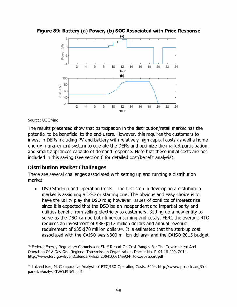
98
Figure 89: Battery (a) Power, (b) SOC Associated with Price Response
Source: UC Irvine
The results presented show that participation in the distribution/retail market has the
potential to be beneficial to the end-users. However, this requires the customers to
invest in DERs including PV and battery with relatively high capital costs as well a home
energy management system to operate the DERs and optimize the market participation,
and smart appliances capable of demand response. Note that these initial costs are not
included in this saving (see section 0 for detailed cost/benefit analysis).
Distribution Market Challenges
There are several challenges associated with setting up and running a distribution
market.
• DSO Start-up and Operation Costs: The first step in developing a distribution
market is assigning a DSO or starting one. The obvious and easy choice is to
have the utility play the DSO role; however, issues of conflicts of interest rise
since it is expected that the DSO be an independent and impartial party and
utilities benefit from selling electricity to customers. Setting up a new entity to
serve as the DSO can be both time-consuming and costly. FERC the average RTO
requires an investment of $38-$117 million dollars and annual revenue
requirement of $35-$78 million dollars30. It is estimated that the start-up cost
associated with the CAISO was $300 million dollars31 and the CAISO 2015 budget
30 Federal Energy Regulatory Commission. Staff Report On Cost Ranges For The Development And
Operation Of A Day One Regional Transmission Organization, Docket No. PL04-16-000. 2014. http://www.ferc.gov/EventCalendar/Files/ 20041006145934-rto-cost-report.pdf
31 Lutzenhiser, M. Comparative Analysis of RTO/ISO Operating Costs. 2004. http://www. ppcpdx.org/Com
parativeAnalysisTWO.FINAL.pdf
99
provides for a revenue requirement of $198.5 million showing an increase of
0.6% a year since 200732. It is expected that DSOs will cost much less than
RTO/ISOs but they will still require significant investment as well as rules and
regulations that will govern these entities.
• Metering and Gathering Data: Since the DERs can each participate in this
market, metering is required for billing and settlement purposes as well as
developing and improving a full distribution system model.
• Control Equipment: For DERs including demand response and microgrids, in
order to be able to be competitive in such markets, they will require
sophisticated control systems capable of responding to market signals and local
needs of the system.
• Tariffs and Interconnection Agreement: In this new paradigm, there needs to be
a change in how the current tariffs and interconnection agreement work
• Protecting the Customer: There might still be a need for a different type of
regulation in order to protect the customer from unreasonably high prices.
• Pricing: The pricing suggested previously is based on the DSO clearing price
which indirectly includes the ISO price; however, there are other pricing schemes
for the retail customers suggested in the literature such as static (flat or time-of
use) and dynamic (real-time pricing, critical peak pricing) pricing.
• Ensure Competitiveness: This issue is related to the overall concept of
deregulation and whether it actually helps reduce prices. FERC analysis showed
that the RTO/ISO impact on the customer bill should be less than 0.5% and
several studies have shown that deregulation might not be the reason for
reduction in electricity prices. Ensuring competitiveness to the extent that results
in lower prices is even a more complicated issue at a distribution level especially
at the start of this new market when the benefits of market participation might
not be evident to investors.
• Narrow Profit Margins: In previous sections, it was shown that DERs can benefit
from ISO market participation. If the DSO market actually results in lower prices,
the profit margin of the DERs will be lower than what previously showed unless
the DSO introduces new products and new markets aimed at responding to local
32 Razeghi, G., Shaffer, B., Samuelsen, S. Impact of electricity deregulation in the state of California.
Energy Policy. 2017; 103: 105-115

100
needs and improving the resiliency of the community for instance use of DERs
for quick and efficient system restoration and black-start of substations33 34.
Suggested Changes In short to medium term, some changes are required to facilitate integration of DERs.
These include simplifying current processes for interconnection agreements with the
utility that also allow export of electricity to the grid that are more economically
beneficial to the customer than existing net-metering. These changes should also cover
microgrids and allow them to export and sell the extra electricity (especially renewable
generation) to the utility, ISO markets, or other retail customers.
Another change that will increase the value of DERs and facilitate their integration is
associated with IEEE 1547. These resources will disconnect from the grid during
outages or fluctuations; however, they can be used during these occurrences to
energize an entire circuit (if large enough), just serve the critical loads through opening
and closing switches or through a dedicated line. These three options are shown in
Figure 90. These resources can also be used to optimize and facilitate system
restoration.
Figure 90: DERs and Microgrids Used During Grid Outages
Source: UC Irvine
33 Xu, Y., Liu, C., Schneider, K. P., Tuffner, F. K., & Ton, D. T. Microgrids for Service Restoration to
Critical Load in a Resilient Distribution System. IEEE Transactions on Smart Grid 2018; 9, 426–437.
34 Xu, Y., Liu, C., Wang, Z., Mo, K., Schneider, K. P., Tuffner, F. K., & Ton, D. T. DGs for Service
Restoration to Critical Loads in a Secondary Network. IEEE Transactions on Smart Grid. 2018; 1.

101
New ISO products and interconnection agreements that facilitate DER integration are
also required which include the “value” of DER instead of their price/cost. This means
that benefits of the DERs (direct and indirect) be included in their bid. For instance, use
of DERs eliminates the 6% transmission losses and defers investments in transmission
upgrades; however, these benefits to the grid do not impact the LCOE of the unit itself.
Using value of the service which includes the benefits to the system (and society)
further increases the penetration and integration of DERs. Cost and benefits of DERs
and microgrids are summarized below.
Costs
• Equipment Capital Costs
• Equipment Operating & Maintenance Costs
• Fuel Input Costs
• Site Preparation Costs
• Increased Market Participation Costs
• Increased Controller Costs
Benefits
• Avoided Criteria Pollutants
• Avoided Greenhouse Gas Emissions
• PV Smoothing
• Increased Renewable Resource Integration
• Optimized DER Dispatch
• Operating Efficiencies
• Reduced Operating Costs
• Reduced Water Usage/Costs
• Peak Shaving/Load Shifting/Demand Charge Reduction
• Energy Charge Reduction
• Reduced Grid Congestion
• Deferred T&D Capacity Investment
• Provision of Ancillary Services & Voltage Support
• Islanding Capability
• Increased Reliability
• Reduced Number and Duration of Outages
• Increased Resiliency
• Reduced Cost of System Restoration after Outages

102
In long-term and in order to have a distribution/retail market, there needs to be new
products and markets in the ISO to include participation of DSOs. There needs to be
rules and regulations for the interactions between DSO and other DSOs, ISO, ESPs and
retail customers, as well as new interconnection agreements between DERs and utility
(which will become the distribution owner) and possible orders and rules to ensure that
the DERs have non-discriminatory access to the distribution system (similar to open
access rule).

103
CHAPTER 7: Benefits of the Project
In this chapter, the benefits of the project for the state of California and especially IOU
ratepayers are discussed. The main benefit of this project is producing a methodology
and strategy that increases, through a systematic use of utility substation resources,
the penetration of distributed energy resources including renewable resources and
energy storage, makes full use of smart grid technologies, and implements automation
and control. Several benefits of the project stem from increased penetration of
distributed energy resources (especially renewable resources such as solar PV) include
reduced criteria pollutants emission, reduced greenhouse gas emissions, increased grid
reliability and increased energy security (due to decreased dependence on foreign oil
and fossil fuels).
Reduced Emissions Optimal dispatch of resources through utility substation automation results in more
efficient operation and ultimately in reduction of the emissions intensity of the grid.
Better grid management by the deployment and application of microgrid control on
distribution circuits emanating from utility substations also results in increased
penetration of renewable resources and complementary technologies further reducing
the emissions from the electricity sector.
Use of distributed energy resources eliminates delivery losses. Energy Information
Administration (EIA) estimates that the average delivery losses (including transmission
and distribution losses) are about 5% in the United States35.For the state of California
the delivery losses are estimated to be 6.58%36. Using distributed energy resources to
replace central generation eliminates this 6.58% energy loss reducing both emissions
and fossil fuel use. .
Furthermore, the electricity generated from the DERs have lower emission factors
compared to the grid (due to high penetration of PV, energy storage, and low emission
factors of the fuel cell). For scenarios simulated, the emission reductions compared to
the base case are calculated.
In order to determine GHG emission reduction due to integration of DERs, the NREL
PVWatts tool37 is used to estimate the year around total electricity production of a grid
35 Energy Information Administration. https://www.eia.gov/tools/faqs/faq.php?id=105&t=3
36 California Public Utilities Commission (CPUC). System Efficiency of California’s Electric Grid. 2017
37 National Renewable Energy Laboratories. PVWatts Calculator. https://pvwatts.nrel.gov/pvwatts.php

104
connected photovoltaic system. The calculator requires the system location and basic
design parameters such as size, module type, and system losses to estimate monthly
and annual electricity production of PV system using an hour by hour simulation over a
period of one year. Table 12 shows the result from the PVWatts calculator for the total
PV installation of 9.89MW associated with scenario 1 results.
Table 12: Annual Electricity Production of 9.89 MW PV
Month AC Energy ( kWh )
January 1,073,450
February 1,094,330
March 1,445,488
April 1,538,395
May 1,599,889
June 1,596,346
July 1,647,779
August 1,632,193
September 1,428,239
October 1,290,149
November 1,096,369
December 992,895
Total 16,435,522
Source: UC Irvine
The emission data were extracted from the Emissions & Generation Resource
Integrated Database (eGRID)38 released by the EPA. It is a comprehensive source of
data on the environmental characteristics of electric power generated in the United
States. From the eGRID2016, California grid average emission rates were found as
shown in Table 13 and the total emissions offset by the PV installation was calculated.
Table 13: Annual Average Emission Factors for CA (kg/MWh)
NOx SOx CO2 CH4 N2O CO2 equivalent
0.257 0.024 239.437 0.015 0.002 240.356
Source: U.S. Environmental Protection Agency (EPA). Emissions & Generation Resource Integrated Database (eGRID) 2016
The GHG reduction associated with deployment of 9.89 MW of PV on the two circuits is
equal to 4,229 mTCO2eq (metric Ton of CO2 equivalent) annually assuming that the
38 U.S. Environmental Protection Agency (EPA). Emissions & Generation Resource Integrated Database
(eGRID). https://www.epa.gov/energy/emissions-generation-resource-integrated-database-egrid.

105
excess PV generation is exported to the grid for full usage and not curtailed. The
transmission loss of 6.58% is also accounted in the offset emissions.
Following the same approach, annual GHG reduction from installation of 15.29 MW of
PV (max RESU results) is equal to 6,537 mTCO2eq. This only accounts for the PV
installation and avoiding delivery losses, and does not take into account the impact of
energy storage operation on reducing emissions. To further investigate the impact of
the different energy storage units (RESU and CES), hourly emission factors of the
average CA grid are used.
An hourly metric ton CO2 per MWh was calculated with the demand data and emissions
data from CAISO39. Each month and year were averaged starting April until mid-
December of 2018 as shown in Figure 91. The midday drop in emissions reflects the PV
deployment and electricity generation. Accounting the dynamics of emissions for 24
hours can give a more accurate and detailed emissions analysis. The 2018 average day
hourly emission factor is shown in black in Figure 91. This profile is used to estimate the
emissions for the 24 hour simulation of the RESU max case and the CES max case in
order to assess the impact of energy storage on shifting the load from high to low
emission intervals.
Figure 91: Average GHG Emission Factor for 2018
Source: UC Irvine
39 California Independent System Operator (CAISO).
http://www.caiso.com/TodaysOutlook/Pages/emissions.aspx

106
The electricity profile without DER, the red profile in Figure 92, is used to determine the
GHG emissions of the baseline using average hourly emission factors shown in Figure
91. The electricity demand profiles with RESUs and CESs from Figure 92 is used to
determine the emissions for two different storage cases. The transmission loss of
6.58% was added to the calculation to account for delivery loss.
Figure 92: Electricity Demand
Source: UC Irvine
The Baseline, RESU case and CES case CO2eq emissions are as listed in Table 14. Given
that the RESU case has more storage (both in terms of power and energy), RESU case
resulted in less CO2eq emissions compared to the CES case. A maximum of 19.7 mTCO2
per day is offset (associated with RESU scenario) and this results in 7,712 mTCO2
reduction per year including the transmission loss of 6.58%. This results in a 34 %
reduction in GHG emissions from these two circuits for the RESU case and 32%
reduction for the CES case. Figure 93 shows the different GHG emission profiles for an
average day for different cases. There is significant reduction in emissions during
midday due to PV electricity generation and the highest emission points during the
evening hours are reduced due to the energy storage operation shifting the loads to
intervals with lower emission intensity.
Table 14: Annual GHG Emission
Baseline CO2eq
Emissions
RESU case CO2eq
Emissions
CES case CO2eq
Emissions
20,971 mTCO2 13,766 mTCO2 14,237 mTCO2
Source: UC Irvine

107
Figure 93: Average Daily GHG Emission Profile
Source: UC Irvine
This analysis further shows the impact and importance of integrating energy storage
with renewable resources to further decrease GHG emissions.
Improved Reliability The reduction in outage duration due to availability of DERs and the controller is
calculated from the results of the circuit-independent test cases. This is then used to
calculate a new SAIDI (System Average Interruption Duration Index), this new SAIDI
number is then compared to the base case SAIDI numbers shown in Table 15 for SCE
territory.
Table 15: SCE Total System Reliability Indices
Year SAIDI SAIFI MAIFI CAIDI
2017 139.73 1.19 1.84 117.19
10 Year Avg(2007-
2017)
130.99 1.00 1.52 130.71
SAIDI = System Average Interruption Duration Index; SAIFI = System Average Interruption
Frequency Index; MAIFI = Momentary Average Interruption Frequency Index; CAIDI = Customer
Average Interruption Duration Index
Source: Southern California Edison. Annual System Reliability Report, Prepared for California Energy Commission. 2017. https://www.sce.com/sites/default/files/inline-files/SCE_2017_Annual_Reliability_Report.pdf
Results of the two emergency scenarios simulated are summarized in Table 16. The
total unserved load was calculated using the original base case demand and the new
demand after load shedding necessary to balance demand and supply during a grid

108
outage. 44% and 43% of the total load was dropped (unserved load) in the CES and
RESU cases, respectively. The loads that were dropped, experience the same outage
duration as the rest of grid while the rest of the load which was served by the DERs do
not experience any interruption. Thus, 60% of the load was not subject to an outage
during the circuit independent operation simulations.
Table 16: 24 Hours Emergency Operation Result
Scenario Demand
(MWh)
New
Demand
(MWh)
Unserved
Load (%)
New
SAIDI
New
SAIFI
CES 210.59 117 44.44 62.09 0.5288
RESU 210.59 120.6 42.73 59.71 0.5085
Source: UC Irvine
The new SAIDI and SAIFI for the two circuits were calculated using Eq (8.1) and Eq
(8.2):
𝑆𝐴𝐼𝐷𝐼𝐴&𝐵 = 𝑆𝐴𝐼𝐷𝐼2017 × 𝑂𝑃𝐴&𝐵 (8.1)
𝑆𝐴𝐼𝐹𝐼𝐴&𝐵 = 𝑆𝐴𝐼𝐹𝐼2017 × 𝑂𝑃𝐴&𝐵 (8.2)
In these equations, 𝑂𝑃𝐴&𝐵is the outage percentage outcome from the 24 hour
simulations. The total interruption duration will reduce by 𝑂𝑃𝐴&𝐵 and the total
interruption frequency will also reduce by 𝑂𝑃𝐴&𝐵. The new SAIDI and SAIFI show an
improvement of over 60% and with a more sophisticated energy management system
per home, it is possible to achieve higher improvements.
The Interruption Cost Estimate (ICE)40 calculator tool is utilized to estimate the
economic benefit of reliability improvement resulted from integration of DERs. The ICE
calculator is a tool developed for those that are interested in estimating interruption
costs and benefits associated with reliability improvements. First the interruption cost
using the 2017 average SAIDI and SAIFI was calculated assuming that the customers
are all residential. Then, the interruption cost using the improved SAIDI and SAIFI are
calculated and compared to the original value. Table 17 shows the results of the
calculation and the economic benefit drawn from the reliability improvement per event
associated with the customers located in the system under study. The interruption cost
is almost halved due to reliability improvement achieved due to deployment of DERs
including the fuel cell.
40 Lawrence Berkeley National Laboratory. Interruption Cost Estimate Calculator.
https://eaei.lbl.gov/tool/interruption-cost-estimate-calculator

109
Table 17: Interruption Cost Estimate
Item Cost
Old Index Interruption Cost $30,846.30
New Index Interruption Cost $13,180.93
Outage Cost Reduction $17,665.37
Source: UC Irvine
Lower Costs An EPRI report41 has shown that the benefits of smart grid technologies outweigh the
required costs with the cost to benefit ratio of 2.8 to 6 for the entire U.S. The main
functionality of the controller is dispatch the resources available to meet the demand.
For business as usual operations which is the majority of the time, the controller
optimizes dispatch of the available resources on the distribution system. This
optimization by definition should result in lower operation costs and a low cost option
for dealing with the intermittencies introduced in the grid by renewable resources. This
is in the context of meeting energy and environmental goals, thus the results are not
compared the least cost generation (such as coal or nuclear).
Modeling and analysis of distribution circuits prior to DER deployment, will also result in
developing a robust strategy on locating the DER across the distribution network and as
a result the assets will neither be stranded nor underutilized. As previously mentioned,
achieving 5% improvement in operation is achievable through optimized dispatch,
which can lower the system cost. If implemented throughout the state, the efficiency of
the grid operation will increase an average of 5% saving almost 13 TWh annually42.
Furthermore, depending solely on distributed resources will eliminate transmission and
distribution losses saving another 15.5 TWh annually for the entire state of California.
As previously mentioned, integration of DERs as described in this project result in
reliability improvement. Using the new calculated SAIDI and SAIFI (Table 16) as inputs
to the ICE calculator demonstrate that this reliability improvement has a benefit of $4.5-
$5.5 per residential customer and has the potential to save $67M-$82M for SCE
customers in total.
Reduced restoration costs is another benefit of smart grid equipped with controller. In
the case of an outage, the controller can help bring the assets up in the most efficient
manner while contributing to overall grid restoration.
41 http://www.epri.com/abstracts/Pages/ProductAbstract.aspx?ProductId=000000000001022519
42 U.S. Department of Energy. State of California Energy Sector Risk Profile.
http://energy.gov/sites/prod/files/2015/05/f22/CA-Energy%20Sector%20Risk%20Profile.pdf

110
Other Benefits In this section, other benefits of this project are described.
Reduced Fossil Fuel Usage
With the integration of DERs, up to 28.5GWh of energy is generated annually in the two
circuits. This implies that less electricity is required from centralized generating units.
California reported state average heat rate for natural gas-fired generating units is 8513
Btu/kWh 43. Using this heat rate and accounting for delivery losses, integration of DERs
in the system under study in this project will result in a reduction of 2.5E11 Btu of
natural usage annually.
Reduced Energy Demand
Results of the project have shown that integration of DERs including distributed
generation, energy storage, energy efficiency, and demand response, all reduce the net
load seen at the substation and reduce the overall electricity demand. This is in addition
of the 6% reduction in load due to avoiding delivery losses. The extent of this reduction
depends on the technology and was described in detail in result of each scenario
simulation in Chapter 6.
Increased Safety
Enhancing automation and control capabilities of the substation, and communication
between the controller and DERs allows for quick resolution and response to faults,
outages, and other issues which results in increased safety for both customers and
utility personnel/workers.
Controlling load further allows for ensuring that the critical loads are being served in
case of an emergency.
Energy Security
Use of renewable energy resources, energy storage, and demand management, reduce
the need for conventional generation and thus reduce the dependence on foreign oil
and gas.
Enhanced Resiliency
Use of DERs, especially if they are allowed to operate during grid outages, can help
improve the resiliency of the grid. These resources can help achieve an optimized and
quick system restoration by energizing part of the grid and help black-start utility
assets. As previously mentioned, used of DERs and microgrids in system restoration has
been covered in multiple studies.
43 Nyberg, M. Thermal Efficiency of Natural Gas-Fired Generation in California: 2017 Update.
2018.California Energy Commission CEC-200-2018-001

111
Reduced RPS Procurement
Implementation of demand response, energy efficiency measures, and energy storage
help reduce the overall net demand or peak net demand and thus reducing the RPS
procurement which is based on demand which can further lower prices. This will result
in reduced purchases and procurement of renewable generation above market prices
solely to meet RPS goals.
Avoided Transmission Upgrade Costs
Retail electricity prices include generation, transmission and distribution costs. Between
59% and 67% of the price is associated with generation of electricity44 and the
remaining 41% to 33% is associated with transmission and distribution costs.
Furthermore, transmission costs are projected to increase 1.2% annually between 2013
and 204044 (compared to 0.6% associated with distribution costs).
Due to increased integration of renewables and the necessity to increase the reliability
and resiliency of the electric grid, utilities continue to increase spending on
transmission. In 2016, total transmission expenditures by utilities included in the FERC
data reached $35 billion, with investment in transmission infrastructure making up 61%
of that total45. With increased penetration and use of DERs, the net load is reduced and
thus the use and stress on the transmission system will be reduced which results in less
frequent upgrades to the transmission system (or at least defer the investment).
44 U.S. Energy Information Administration. Annual Energy Outlook 2015 with projections to 2040. 2015.
https://www.eia.gov/outlooks/aeo/pdf/0383(2015).pdf
45 U.S. Energy Information Administration. Federal Energy Regulatory Commission Financial Reports
112
CHAPTER 8: Conclusions
In this project, the GMC software specifications, established under a U.S. Department of
Energy program, were used to develop a controller which was simulated on two 12kV
distribution circuits at a Southern California Edison (SCE) substation using the OPAL-RT
simulation platform. The two distribution circuits were previously part of the DOE Irvine
Smart Grid Demonstration (ISGD) project led by SCE in collaboration with APEP as the
research partner and project host. The data collected from the ISGD project were used
to validate and inform the models developed.
Developed models of the distribution circuits and the controller were used to simulate
future viable scenarios in order to assess the impact of high PV penetration, energy
storage, electric vehicles, and demand response on the operation of the distribution
system and improving reliability. Furthermore, the viability of a distribution/retail
electricity market was assessed and the fundamentals of such markets introduced.
Major Findings
• Higher DER (including PV) penetration can be achieved with substation control
and automation. Results of the simulations demonstrated that using the
controller to manage the operation of DERs in distribution circuits in an optimized
manner increases the PV hosting capacity of the distribution system without any
upgrade. Addition of energy storage units and optimizing their operation can
further increase PV penetration in the distribution system as was demonstrated
in the RESU and CES cases.
• CES is a more economic approach for achieving high PV penetration and GHG
reduction that residential storage. RESU and CES cases simulated and assessed
in this project, resulted in similar PV penetration (37.5% and 35.4%,
respectively). However, using CES units, this PV penetration was achieved with
less battery energy storage deployed both in terms of power and energy
capacity, and this represents a more economic approach since battery energy
storage is capital intensive. The RESU case includes more energy storage and
has slightly higher PV penetration, it results in more GHG reduction (34% versus
32% for the CES). However, RESU cases result in 355 mTCO2eq reduction per
MWh of installed energy storage, while CES cases result in 660 mTCO2eq
reduction per MWh of installed energy storage demonstrating that CES approach
is a superior approach in terms of GHG reduction (and cost).
• DERs can be used to serve the needs of the larger grid. Although DERs mainly
serve the local needs of the distribution system, they can be used to serve the
needs of the larger grid, and help alleviate the duck curve in the state of

113
California particularly. The results of the simulations showed that a large battery
deployed at the distribution substation helps reduce the depth of the duck curve
by curbing PV export to the grid. Demand response, on the hand, helps the duck
curve by reducing the demand later in the afternoon and reducing the need for
high ramping rates during these times.
• Fuel cell deployment at the substation improves reliability of the system. As
demonstrated by the results of the simulations, having a source of firm power at
the substation helps better manage supply and demand, and reduce unserved
load during grid outages. This results in significant improvement of SAIDI and
SAIFI of the system.
• DER market participation is beneficial to the grid as well as DER
owner/aggregator. Cost/benefit analysis performed in this project showed that
overall market participation increases the benefit to cost ratio of DERs making
them more attractive to investors. The extent of the benefits and most lucrative
markets for DERs depends on the size of the resource, its location, and its
ownership. For example, for RESUs that are behind the meter and owned by a
residential customer, the majority of DER benefits were associated with retail
load-shifting and frequency regulation. For the circuit battery, however, which is
much larger than a RESU and it is on the utility side, the benefits were
associated with wholesale day-ahead market participation, non-spinning reserve,
as well as frequency regulation. Both of these resources were able to serve the
grid needs since they were cleared and used various wholesale markets.
• Participation of retail customers in distribution electricity markets can benefit
them financially. By directly participating in a distribution market, retail
customers will see the real-time electricity market prices and will be able to
respond to such prices accordingly to reduce their overall energy bill. Results of
the simulation demonstrated that this distribution/retail market can indeed help
reduce the electricity bill of retail customers. Furthermore, with real-time flowing
down to the retail customer, the flexibility of electricity demand is increased
providing another benefit to the overall grid.
Recommendations and Future Work
• Use of distribution circuits as microgrids should be further investigated. In this
project, although emergency cases were studied, they were focused on
balancing supply and demand without any electricity import from the grid.
Transition to an islanded mode operation and resynchronization should be
further studied.
• Use of fuel cells in system restoration and recovery can be further studied which
requires a detailed analysis of fuel cell operation in grid-forming.

114
• Standardize, simplify, and streamline the process for interconnection
agreements, and allow export of electricity to the grid that is more economically
beneficial to the customer than allowed by existing net-metering rules.
• Allow DERs to export and sell the electricity to the utility, ISO markets, or retail
customers.
• Rethink anti-islanding requirements and allow for intentional islands.
• Establish ISO products that are specific to DERs and microgrids enabling DERs
with direct and indirect benefits included in the bid.
• Legislation is required in order to establish competitive distribution/retail markets
which requires more research on the impact of such markets in long term on
prices.

115
LIST OF ACRONYMS
Term Definition
APEP Advanced Power and Energy Program
AS Ancillary Services
BA Balancing Authority
BC Breaker Controller
CAISO California Independent System Operator
CCA Community Choice Aggregation
CES
Community Energy Storage. This is a battery energy storage units
deployed close to the transformer and serving all the customers
served by that particular transformer
DAM Day-Ahead Market
DER Distributed Energy Resource
DERP Distributed Energy Resource Provider
DNU Delivery Network Upgrade
DR Demand Response
DSO Distribution System Operator
eGRID Emissions & Generation Resource Integrated Database
EMS Energy Management System
EMT Electromagnetic Transient
EPIC (Electric
Program
Investment
Charge)
The Electric Program Investment Charge, created by the California
Public Utilities Commission in December 2011, supports
investments in clean energy technologies that benefit electricity
ratepayers of Pacific Gas and Electric Company, Southern California
Edison Company, and San Diego Gas & Electric Company.
EVSE Electric Vehicle Service Equipment
FERC Federal Energy Regulatory Commission
GC Generation Controller
GHG Greenhouse Gas
GIA Generator Interconnection Agreement

116
Term Definition
GIDAP Generator Interconnection and Deliverability Allocation Procedure
GIP Generator Interconnection Procedure
GMC Generic Microgrid Controller.
HIL Hardware-in-the-Loop
IEEE 2030.7 IEEE standard for microgrid controller development
IC Interconnection Customer
IOU Investor-Owned Utility
IR Interconnection Request
IS Interconnection Service
ISGD Irvine Smart Grid Demonstration.
ISO Independent System Operator
LC Load Controller
LCR Local Capacity Requirement
LMP Locational Marginal Price
LSE Load Serving Entity
MCP Market Clearing Price
Microgrid
A group of interconnected loads and distributed energy resources
within clearly defined electrical boundaries that acts as a single
controllable entity with respect to the grid. A microgrid can connect
and disconnect from the grid to enable it to operate in both grid-
connected or island-mode.’’
MILP Mixed Integer Linear Programming
MMC Master Microgrid Controller
MRTU Market Redesign and Technology Upgrade
NEM Net Energy Metering
Nested
Microgrid
Interconnection one or more nanogrids to a microgrid representing
themselves as a single controllable entity to the microgrid
NGR Non-Generating Resource
PAFC Phosphoric Acid Fuel Cell

117
Term Definition
PDR Proxy Demand Resource
PEV Plug-in Electric Vehicle
PNode Price Node
POI Point of Interconnection
PV Photovoltaic
RA Resource Adequacy
RESU
Residential Energy Storage Unit. This system refers to a PV/battery
combination on the same inverter deployed on the customer side
of the meter
RPS Renewable Portfolio Standard
RTM Real-Time Market
RTO Regional Transmission Operator
RTUC Real-Time Unit Commitment
RUC Residual Unit Commitment
SAIDI
System Average Interruption Duration Index which is commonly
used as a reliability indicator by electric power utilities. SAIDI is the
average outage duration for each customer served
SAIFI
System Average Interruption Frequency Index is the average
number of sustained interruptions per consumer during the year. It
is the ratio of the annual number of interruptions to the number of
consumers.
SC Storage Controller/ Scheduling Coordinator
SCE Southern California Edison. One of three Investor Owned Utilities in
the state of California
SCUC Security Constraint Unit Commitment
SGIP Self-Generation Incentive Program
Smart grid
Smart grid is the thoughtful integration of intelligent technologies
and innovative services that produce a more efficient, sustainable,
economic, and secure electrical supply for California communities.
SOC State of Charge
TEV Testing, Evaluation, and Verification

118
Term Definition
TOT Transmission Owner’s Tariff
TOU Time of Use
TP Transmission Plan
TPP Transmission Planning Process
TSO Transmission System Operator
UCI University of California, Irvine
UCIMG University of California, Irvine Microgrid
VNM Virtual Net Metering
WDAT Wholesale Distribution Access Tariff
ZNE Nero Net Energy

119
REFERENCES
Akbari, A., Carrera-Sospedra, M., Hack, R., McDonell, V., & Samuelsen, S. (2015). Final
Project Report Realistic Application and Air Quality Implications of distributed
generation and combined heat and power. California Energy Commission.
Retrieved from https://www.energy.ca.gov/2015publications/CEC-500-2015-
032/CEC-500-2015-032.pdf
California Independent System Operator. (2012). Appendix EE: Large generator
interconnection agreement for interconnections requests processed under the
generator interconnection and deliverability allocation procedures. Retrieved
from https://www.caiso.com/Documents/TariffAppendixEE_Nov5_2012.pdf
California Independent System Operator. (2013). Appendix FF: Small generator
interconnection agreement for interconnection requests under the generator
interconnection and deliverability allocation procedures. Retrieved from
http://www.caiso.com/Documents/AppendixFF_SmallGeneratorInterconnetionAgr
eement-GIDAP_Dec3_2013.pdf
California Independent System Operator. (2014). Appendix DD: Generator
Interconnection and Deliverability Allocation Procedures (GIDAP). Retrieved from
http://www.caiso.com/Documents/AppendixDD_GeneratorInterconnection_Deliv
erabiltyAllocationProcessDec19_2014.pdf
California Independent System Operator (2016). CAISO time-of-use periods analysis.
Retrieved from
http://docs.cpuc.ca.gov/PublishedDocs/Efile/G000/M157/K905/157905349.PDF
California Public Utilities Commission. (2012). Decision adopting a code of conduct and
enforcement mechanisms related to utility interactions with community choice
aggregators, pursuant to Senate Bill 790. Retrieved from
http://www.cpuc.ca.gov/general.aspx?id=2567
California Public Utilities Commission. (2017). System efficiency of California’s electric
grid. Retrieved from
http://www.cpuc.ca.gov/uploadedFiles/CPUC_Public_Website/Content/About_Us/
Organization/Divisions/Policy_and_Planning/PPD_Work/PPD_Work_Products_(20
14_forward)/System_Efficiency_Report PPD_May_24_Final.pdf
California Public Utilities Commission. (2019). Registered Electric Service Providers.
Retrieved from https://apps.cpuc.ca.gov/apex/f?p=511:1
Clear Edge Power (2013). Electric Load - Following Capability of the PureCell ® Model
400 Fuel Cell System, (January). Retrieved from
120
http://www.clearedgepower.com/downloads/files/whitepapers/Electric_Load_Foll
owing.pdf
Conti, S., Nicolosi, R., Rizzo, S. A., & Zeineldin, H. H. (2012). Optimal Dispatching of
Distributed Generators and Storage Systems for MV Islanded Microgrids. IEEE
Transactions on Power Delivery, 27(3), 1243–1251.
https://doi.org/10.1109/TPWRD.2012.2194514
De Martini, P., & Kristove, L. (2014). 21st Century Electric Distribution System
Operations. Retrieved from http://resnick.caltech.edu/docs/21st.pdf
De Martini, P., & Kristove, L. (2015). Distribution system in a high distributed energy
resources future. Retrieved from https://emp.lbl.gov/sites/all/files/lbnl-
1003797.pdf
De Martini, P., & Kristove, L. (2014). 21st Century Electric Distribution System
Operations. Retrieved from http://resnick.caltech.edu/docs/21st.pdf
Denholm, P., O’Connell, M., Brinkman, G., & Jorgenson, J. (2015). Overgeneration from
Solar Energy in California. A Field Guide to the Duck Chart, (November).
https://doi.org/10.2172/1226167
Electric Power Research Institute. (2011). Estimating the Costs and Benefits of the
Smart Grid. Retrieved from
https://www.epri.com/#/pages/product/000000000001022519/?lang=en-US
Electric Power Research Institute. Storage Value Estimation Tool (StorageVET).
Retrieved from https://www.storagevet.com/
Environmental Protection Agency. (2018). Emissions & Generation Resource Integrated
Database (eGRID). Retrieved from https://www.epa.gov/energy/emissions-
generation-resource-integrated-database-egrid
Lawrence Berkeley Lab. Interruption Cost Estimate Calculator. Retrieved from
https://eaei.lbl.gov/tool/interruption-cost-estimate-calculator
Li, M., Zhang, X., Li, G., & Jiang, C. (2016). A feasibility study of microgrids for reducing
energy use and GHG emissions in an industrial application. Applied Energy, 176,
138–148. https://doi.org/10.1016/J.APENERGY.2016.05.070
National Renewable Energy Laboratory. PVWatts Calculator. Retrieved from
https://pvwatts.nrel.gov/pvwatts.php
Nyberg, M. (2018). Thermal Efficiency of Natural Gas-Fired Generation in California:
2018 Update. California Energy Commission. CEC-200-2018-011

121
Pyper, J. (2018). It’s Official. All New California Homes Must Incorporate Solar.
Retrieved from https://www.greentechmedia.com/articles/read/solar-mandate-
all-new-california-homes#gs.h2lwiSJC
Razeghi, G., Shaffer, B., & Samuelsen, S. (2017). Impact of electricity deregulation in
the state of California. Energy Policy, 103.
https://doi.org/10.1016/j.enpol.2017.01.012
Razeghi, G. (2013). The Development and Evaluation of a Highly-Resolved California
Electricity Market Model to Characterize the Temporal and Spatial Grid,
Environmental, and Economic Impacts of Electric Vehicles. University of
California, Irvine.
Razeghi, G., Brouwer, J., & Samuelsen, S. (2016). A spatially and temporally resolved
model of the electricity grid—Economic vs environmental dispatch. Applied
Energy, 178, 540–556. https://doi.org/10.1016/j.apenergy.2016.06.066
Razeghi, G., Gu, F., Neal, R., & Samuelsen, S. (2018). A generic microgrid controller:
Concept, testing, and insights. Applied Energy, 229, 660–671.
https://doi.org/https://doi.org/10.1016/j.apenergy.2018.08.014
Razeghi, G., Neal, R., & Samuelsen, S. (2016). Generic Microgrid Controller
Specifications. Technical Report to the US Department of Energy. Retrieved from
http://www.apep.uci.edu/Research/PDF/Microgrid/Generic_Microgrid_Controller_
Specifications_Oct_2016_Razeghi_Neal_Samuelsen_032318.pdf
Razeghi, G., & Samuelsen, S. (2016). Impacts of plug-in electric vehicles in a balancing
area. Applied Energy, 183, 1142–1156.
https://doi.org/10.1016/j.apenergy.2016.09.063
Report, F. (2017). California Solar Initiative RD & D Program Process Evaluation.
Retrieved from
file:///C:/Users/jjl/Desktop/Papers/CSI_RDD_Evaluation_Report_FINAL_051117.p
df
Samuelsen, S., & Brouwer, J. (2013). Development and analysis of a progressively
smarter distribution system, Final Report, Submitted to CSI RD&D Program
Administrator.
Shaffer, B., Tarroja, B., & Samuelsen, S. (2015). Dispatch of fuel cells as transmission
integrated grid energy resources to support renewables and reduce emissions.
Applied Energy, 148(x), 178–186.
https://doi.org/10.1016/j.apenergy.2015.03.018

122
Southern California Edison. (2016). Annual System Reliability Report. Retrieved from
ftp://ftp.cpuc.ca.gov/ElecReliabilityAnnualReports/2016/SCE_2016_
Annual_Reliability_Report.pdf
Southern California Edison. (2016). Final Technical Report: Irvine Smart Grid
Demonstration, a Regional Smart Grid Demonstration Project. Retrieved from
https://www.energy.gov/sites/prod/files/2017/01/f34/ISGD Final Technical
Report_20160901_FINAL.pdf
U.S. Department of Energy. State of California Energy Sector Risk Profile. Retrieved
from http://energy.gov/sites/prod/files/2015/05/f22/CA-Energy Sector Risk
Profile.pdf
U.S. Energy Information Administration. (2017). California wholesale electricity prices
are higher at the beginning and end of the day. Retrieved from
https://www.eia.gov/todayinenergy/detail.php?id=32172
U.S. Energy Information Administration. (2018). Electric Power Annual. Retrieved from
https://www.eia.gov/electricity/annual/
U.S. Energy Information Administration. (2018). Electricity residential retail choice
participation has declined since 2014 peak. Retrieved from
https://www.eia.gov/todayinenergy/detail.php?id=37452
U.S. Energy Information Administration. (2019). How much electricity is lost in
electricity transmission and distribution in the United States? Retrieved from
https://www.eia.gov/tools/faqs/faq.php?id=105&t=3
Xu, Y., Liu, C., Schneider, K. P., Tuffner, F. K., & Ton, D. T. (2018). Microgrids for
Service Restoration to Critical Load in a Resilient Distribution System. IEEE
Transactions on Smart Grid, 9, 426–437.
https://doi.org/10.1109/tsg.2016.2591531
Xu, Y., Liu, C., Wang, Z., Mo, K., Schneider, K. P., Tuffner, F. K., & Ton, D. T. (2018).
DGs for Service Restoration to Critical Loads in a Secondary Network. IEEE
Transactions on Smart Grid, 1. https://doi.org/10.1109/tsg.2017.2743158

A-1
APPENDIX A: Test Case Templates
This appendix provides the test case templates.

A-2
Template A-1: Scenario (test case) template

A-3

A-4
Template A-2: High PV Scenarios
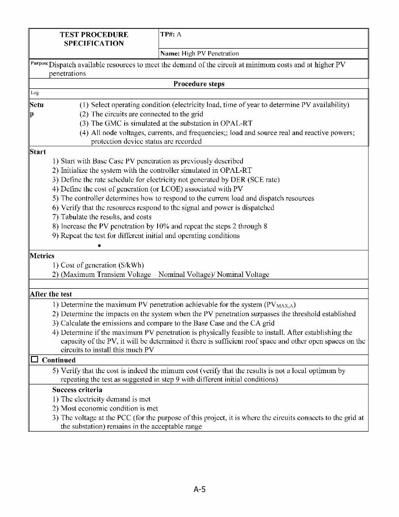
A-5
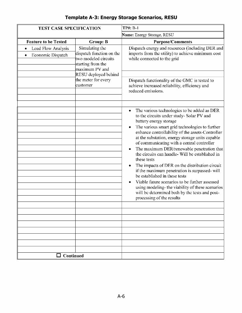
A-6
Template A-3: Energy Storage Scenarios, RESU

A-7

A-8

A-9
Template A-4: Energy Storage Scenarios, CES

A-10

A-11

A-12
Template A-5: Energy Storage Scenarios, Substation Battery

A-13

A-14

A-15
Template A-6: Demand Response Scenarios, HVAC and Smart Appliances

A-16

A-17
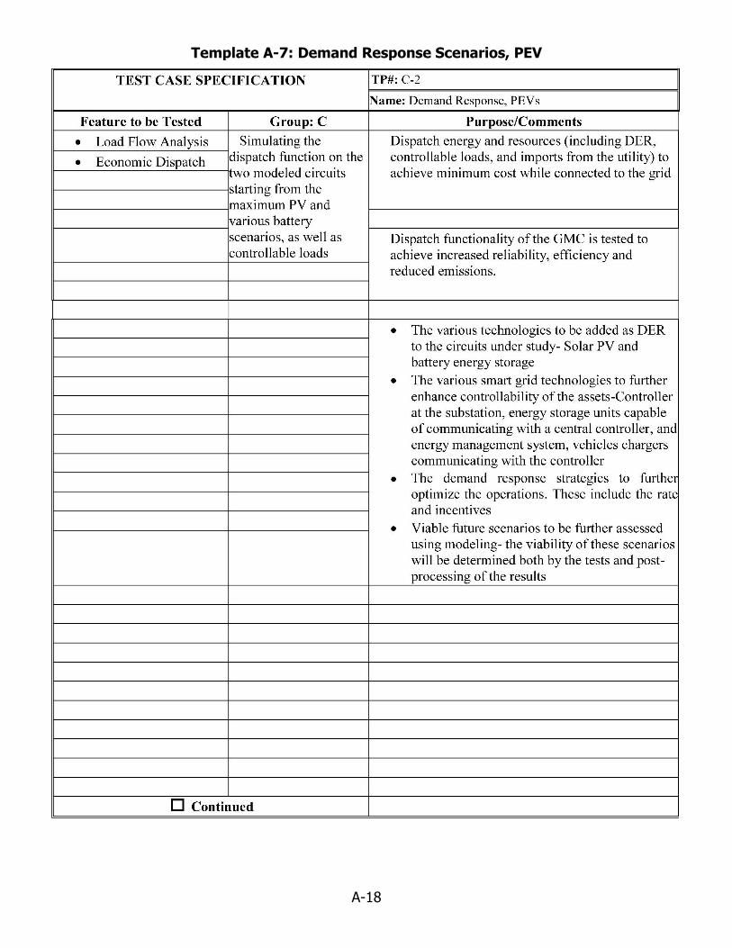
A-18
Template A-7: Demand Response Scenarios, PEV

A-19

A-20

A-21
Template A-8: Circuit-Independent

A-22

A-23

B-1
APPENDIX B: Interconnection/Market Overview
Generator/Resource Interconnection Overview This section provides an overview of the generator interconnection processes in
Southern California Edison (SCE) territory. Understanding these processes requires
some background in the electric power system and its market structure, as well as in
the procedural requirements for such interconnections.
In the past, Investor Owned Utilities (IOU) such as SCE were vertically integrated
monopolies, owning and responsible for all generation, transmission, and distribution
assets, as well as for metering, crediting and billing retail customers. The IOUs were
(and are) regulated by the California Public Utilities Commission (CPUC). Under what
has been called deregulation, the generation business was largely removed from the
monopoly and opened to competition. Many functions which were previously internal
coordinated activities at SCE such as generation and transmission planning had to be
transitioned to open market based processes overseen by either the CPUC or the newly
created California Independent System Operator (CAISO). The CAISO operates the
transmission systems owned by SCE, PG&E, SDG&E, and Nevada’s VEA. The CAISO
borders define one Control Area (CA) in the Western Interconnect for which CAISO is
the Balancing Authority (BA). A BA is responsible to manage internal load and
generation so as to maintain the scheduled power interchanges at its Points of
Interconnection (POI) to other CAs, such as LADWP. These power interchanges are
scheduled on an hourly step-change basis.
Retail customers are served by Load Serving Entities (LSE) including, in the CAISO area,
the three Investor Owned Utilities (IOU) PG&E, SCE and SDG&E, some 2446 Energy
Service Providers (ESP) and by Community Choice Aggregators (CCA)47. Each LSE is
required by the CPUC to prove they have under contract sufficient generating capacity
for Resource Adequacy (RA) which is defined as 115% of their Load Forecast on a 1 in
2 year basis. In addition, they must procure energy to meet their actual load on an
economic basis. Most of these RA and energy needs are obtained via bilateral contracts
(following an open RFO solicitation) and the remainder are obtained on the market
operated by the CAISO. Each LSE submits both an annual and a Long Term
Procurement Plan (LTPP) to the CPUC to prove they meet these and other
requirements.
46 https://apps.cpuc.ca.gov/apex/f?p=511:1:
47 http://www.cpuc.ca.gov/general.aspx?id=2567

B-2
A capacity contract (satisfying RA requirements) pays the generator for having, for
example, 100 MW of deliverable capacity online at a given time, and pays them a
certain rate for energy actually delivered during that time. However the LSE may
actually buy the energy it uses during that time from a more economic generator, or
from a renewable generator to meet its RPS requirements, meaning that our RA
generator with 100 MW capacity available may be delivering substantially less power
during that time. At the same time, LSEs may prefer energy contracts with generators
able to meet RA requirements. Being a more-or-less free market process, a wide variety
of purchase contracts can exist.
The CAISO market defines generator power delivery as occurring at “Pricing Nodes” or
PNodes which are substations at which transmission becomes distribution. Load is
priced at an energy weighted average of all the delivery nodes of the LSE. The price of
power offered at one of these Pnodes must include three components: (1) power
delivered at the PNodes, (2) I2R losses caused by the power exchange, and (3) a
charge related to transmission system congestion occasioned by the power exchange in
question. This method puts remote and local resources on an even playing field. The
whole market scheme is based on the concept of Locational Marginal Price (LMP). If there
was no transmission congestion and any buyer could access any seller, then the LMP
would be the same everywhere (neglecting the I2R losses which are small). However,
transmission limits prevent the next cheapest available power from getting just
anywhere on the grid. The LMP reflects the cost of the next MWh at a given node when
that power is provided with a generator dispatch that results in the lowest overall
system cost, consistent with system physical constraints and security requirements and
thus the terms “security-constrained unit commitment” and “security constrained
economic dispatch (SCED)”.
The CAISO area is divided into ten local areas (Figure B-1) based on significant
transmission constraints between major pockets of load. A portion of the RA procured
by the LSEs must be within these local areas due to transmission constraints as
determined by the CAISO conservatively based on a 1 in 10 year load with certain
transmission contingencies. That portion is referred to as Local Capacity Requirement
(LCR).
California is, in general, a net importer of power, and the capacity of the interchanges
to other BAs and other states is allocated to the LSEs for purposes of meeting their RA
requirements from generators outside of CAISO.

B-3
Figure B-1: CAISO's Local Areas
Source: California Independent System Operator, 2019 Local Capacity Area Technical Study
(https://www.caiso.com/Documents/2019LocalCapacityRequirementsFinalStudyManualdocx.pdf)
Generators count for RA based on their Net Qualifying Capacity (NQC) which includes
transmission deliverability, “technical factors” for renewables, performance history and
other factors.
In addition to the energy and RA markets of the LSEs, the CAISO identifies and
determines the quantity of ancillary services (AS) required for reliability48 and the AS
48 CAISO reliability requirements comply with those of NERC, WECC and the NRC.
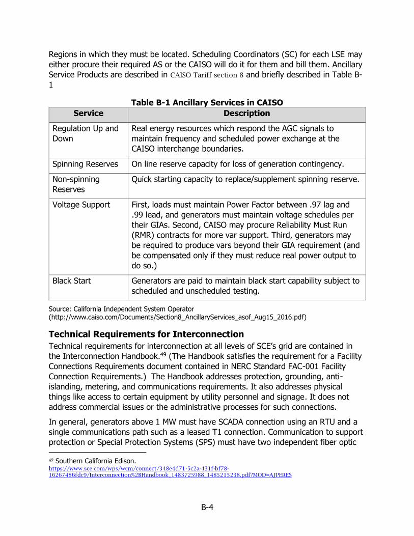
B-4
Regions in which they must be located. Scheduling Coordinators (SC) for each LSE may
either procure their required AS or the CAISO will do it for them and bill them. Ancillary
Service Products are described in CAISO Tariff section 8 and briefly described in Table B-
1
Table B-1 Ancillary Services in CAISO
Service Description
Regulation Up and
Down
Real energy resources which respond the AGC signals to
maintain frequency and scheduled power exchange at the
CAISO interchange boundaries.
Spinning Reserves On line reserve capacity for loss of generation contingency.
Non-spinning
Reserves
Quick starting capacity to replace/supplement spinning reserve.
Voltage Support First, loads must maintain Power Factor between .97 lag and
.99 lead, and generators must maintain voltage schedules per
their GIAs. Second, CAISO may procure Reliability Must Run
(RMR) contracts for more var support. Third, generators may
be required to produce vars beyond their GIA requirement (and
be compensated only if they must reduce real power output to
do so.)
Black Start Generators are paid to maintain black start capability subject to
scheduled and unscheduled testing.
Source: California Independent System Operator (http://www.caiso.com/Documents/Section8_AncillaryServices_asof_Aug15_2016.pdf)
Technical Requirements for Interconnection
Technical requirements for interconnection at all levels of SCE’s grid are contained in
the Interconnection Handbook.49 (The Handbook satisfies the requirement for a Facility
Connections Requirements document contained in NERC Standard FAC-001 Facility
Connection Requirements.) The Handbook addresses protection, grounding, anti-
islanding, metering, and communications requirements. It also addresses physical
things like access to certain equipment by utility personnel and signage. It does not
address commercial issues or the administrative processes for such connections.
In general, generators above 1 MW must have SCADA connection using an RTU and a
single communications path such as a leased T1 connection. Communication to support
protection or Special Protection Systems (SPS) must have two independent fiber optic 49 Southern California Edison. https://www.sce.com/wps/wcm/connect/348e4d71-5c2a-431f-bf78-16267486fdc9/Interconnection%2BHandbook_1483725988_1485215238.pdf?MOD=AJPERES

B-5
lines to the SCE point of connection. These can also support the required SCADA
communications.
Procedures for Interconnecting Generators to SCE’s Grid
A generator seeking an interconnection is called an Interconnection Customer (IC) who
makes an Interconnection Request (IR) to receive Interconnection service (IS) via
Interconnection Facilities (IF) under a Generator Interconnection Agreement (GIA). An
IR from an IC traditionally results in a study process to determine the impact of the
interconnection on the system and the facilities necessary to make a safe
interconnection and mitigate such impacts. The study process will to ensure an
adequate but not excessive level of study for the particular IR.
In California and most states, the grid is divided into a distribution system under state
jurisdiction (CPUC) for serving retail customers and a transmission system under federal
jurisdiction (FERC) for interstate commerce in wholesale bulk power. The
subtransmission system may fall into either category depending on whether it creates a
parallel path to the transmission system or a separate system just for distribution to
customers. SCE’s subtransmission system is almost all part of CPUC jurisdiction while
PG&E and SDG&E’s subtransmission systems are predominantly FERC/CAISO
jurisdictional.
Generator interconnection processes depend on which part of the system the
connection is made and to whom the power is sold. In SCE territory there are three
major processes:
A. The CAISO TOT GIDAP for connection to the transmission system for wholesale
power
B. The SCE WDAT GIP for connection to the distribution or subtransmission system
for wholesale power
C. SCE Rule 21 for connection to the distribution or subtransmission system for self-
generation or for Net Energy Metering at any voltage level
These three processes are discussed in the following sections.
CAISO TOT
Connecting to the SCE’s FERC jurisdictional CAISO controlled transmission grid for
purposes of sale on FERC Jurisdictional CAISO market is governed by the CAISO
Transmission Owner’s Tariff (TOT). Appendix DD Generator Interconnection and
Deliverability Allocation Procedure (the GIDAP)50 describes this in details.
50 California Independent System Operator.
http://www.caiso.com/Documents/AppendixDD_GeneratorInterconnection_DeliverabiltyAllocationProcess
Dec19_2014.pdf

B-6
As shown in Figure B-2, the process of interconnection to the CAISO grid is divided into
four phases: (1) The Interconnection Request, (2) The interconnection Study, (3) The
Generator Interconnection Agreement, and (4) New Resource Implementation.
Figure B-2 CAISO Interconnection Process Overview
Source: California Independent System Operator. http://www.caiso.com/planning/Pages/GeneratorInterconnection/Default.aspx
For transmission level interconnection, four tracks are available within this process: (1)
The Queue Cluster Process, (2) The Independent Study Process, (3) The Fast Track
Process, and (4) the 10 kW Inverter Process. Their applicability is provided in Table B-2.
Table B-2: Tracks within the TOT interconnection process
Track Submit IR Applicable to Length
Queue Cluster In April All 28 months
Independent
Study
Anytime Electrically
independent of
other
generators
8 months for
EO
Fast Track Anytime <=5MW 10 weeks
10 kW Inverter Anytime 10 kW
Inverters with
UL 1741
10 weeks
Source: California Independent System Operator. http://www.caiso.com/planning/Pages/GeneratorInterconnection/Default.aspx
A comparison of the timelines associated with the three tracks is given in Figure B-3
below. (The 10 kW Inverter process is a subset of the Fast Track.) Note that
throughout the various processes, there are requirements for financial security postings
to make sure the IR remains real and to fund ongoing study activity. Similarly, there are
requirements to show “Site Exclusivity” meaning the generator has the right to build on
a site, and similar showings of progress.

B-7
Figure B-3: Interconnection Timelines Summary
Source: California Independent System Operator. Interconnection Application Options and Process. https://www.caiso.com/Documents/1-2018InterconnectionApplicationRequirements-Options.pdf
The main difference between these tracks is the degree of study required. In general,
every generator impacts the common grid and may contribute to the need for grid
upgrades. This leads to the need for IRs to be studied together which has led to the
Cluster study process as the default way of performing the required studies. If,
however, a particular generator can demonstrate “Electrical Independence” as to
reliability and local deliverability concerns, it may be interconnected as an Energy Only
generator under the Independent Study Process (ISP). If Full or Partial Deliverability
Status is desired, that will be assessed later as part of the Cluster Study then in
progress. The Fast Track and 10 kW Inverter tracks are limited to small EO generators.
Deliverability Status
An understanding of interconnection requires an understanding of “Deliverability
Status.” Generators may have one of three Deliverability Status designations: Full
Capacity, Partial Capacity, or Energy Only (EO). Only generators with full or partial
deliverability status may participate in the capacity (RA) market. Any generator can
participate in the energy market.
“Deliverability” refers to the ability of generated power to be delivered to customers
over the transmission network. Generators under study may be able to do this with
capacity in the existing transmission plan or may require network upgrades. Network
upgrades may be classified as driven by reliability concerns, mostly short circuit and
stability but also some load flow. Deliverability network upgrade (DNU) is further

B-8
divided into local (LDNU) and area (ADNU). LDNU involves transmission facilities near
the point of interconnection (POI) which are typically overloaded by one or a few
generators. ADNU are typically overloads between major CAISO local areas and are
driven by contributions of 20 or more generators.
The Transmission Planning Process (TPP) proceeds annually in parallel with the GIDAP
resulting in a current Transmission Plan (TP) at all times. This transmission plan
includes some excess area delivery capability which is allocated to those ICs whose IR
requests full or partial deliverability so as to participate in the capacity market. The
allocation is based on the interconnection customer’s progress in terms of permitting,
financing, and siting.
Because the transmission planning process is repeated annually, there is an opportunity
to reassess available TP deliverability every year.
The Interconnection Request Process
The forms for making a generator interconnection request under the TOT and
submitting associated data can be found in CAISO forms and documents51. The
preferred method of submitting IRs is via the online Resource Interconnection
Management System (RIMS)52. The IR application requires fairly extensive technical
information about the proposed resource. RIMS is used to track the status of all of the
steps involved between application and commercial operation. Once an IR is accepted,
it is assigned a queue position. A listing of all IRs by queue position (which does not
provide the name of the requesting entity) can be found by searching the CAISO
Website for the title “Interconnection Queue” and selecting the document with a title of
“ISO Generator Interconnection Queue.
The Study Process
The main track involving the most generators is the Queue Cluster study process. The
studies include all IRs in the Queue, which is open from April 1 to April 30 each year.
Since the overall process takes 28 months, there will be a number of staggered studies
going on at any time.
The studies are divided into a Phase I and Phase II. Phase I determines a good faith
estimate of IF, a cap on RNU and LDNU costs, and an informational estimate of ADNU
costs. Phase I is followed by meetings at which minor changes can be made and at
which the IC must choose between Option A and Option B as to ADNU costs if full or
partial deliverability status was requested in the IR.
51 California Independent System Operator.
https://www.caiso.com/Pages/documentsbygroup.aspx?GroupID=055cb684-2a53-4a98-9657-40cbd1d87ba2
52 California Independent System Operator. http://www.caiso.com/Documents/RIMSUserGuide.pdf

B-9
“Option A” is a choice to rely on TP capacity allocation, which, if inadequate, drops the
interconnection customer to energy only deliverability status. Option B means
committing to funding (with eventual repayment via TAC53) of their share of the actual
cost of ADNU.
If a generator can show that it is electrically independent of other generators such that
there will be no sharing of RNU and LDNU, it is eligible for the Independent Study
Process (ISP). An ISP Interconnection Request can be submitted at any time. An ISP
study consists of a System Impact Study (SIS) and a Facilities Study (FS). (These were
the traditional parts of an interconnection study before the Cluster Study approach.) It
results in the interconnection customer being assigned EO deliverability status with Full
or Partial deliverability, if requested, being rolled into the deliverability assessment of
whichever Cluster Study is appropriate based on timing. The normal time for the ISP is
8 months (to EO status) as opposed to 28 months for the Cluster process.
A Fast Track process, including the 10 kW Inverter process, is available for small (5 MW
or less) generators and can be accomplished in as little as ten weeks.
Generator Interconnection Agreement
The Generator Interconnection Agreement (GIA) follows the format provided in either
CAISO Tariff Appendix EE54 for large generators or FF55 for small (<20 MW) generators.
A draft agreement is then provided to the interconnection customer for negotiations.
There is a process for dispute resolution if necessary.
The agreement covers responsibilities of each party for the construction, testing,
operation, and maintenance of the generating and interconnection facilities. It
formalizes the results of the studies and governs the subsequent physical
implementation.
New Resource Implementation
The Interconnection Request, Study and Generator Interconnection Agreement are, in a
way, just paper. There still needs to be an actual process for connecting the physical
generator and making it available for CAISO market operations. The CAISO identifies six
“buckets” of required submittals to get to actual synchronous connection to their grid
and to the ultimate goal of the Commercial Operation Date (COD). The dates for CAISO
53 The Transmission Access Charge (TAC) is the part of the customer’s bill that pays for transmission
costs.
54 California Independent System Operator. https://www.caiso.com/Documents/TariffAppendixEE_Nov5_2012.pdf
55 California Independent System Operator.
http://www.caiso.com/Documents/AppendixFF_SmallGeneratorInterconnetionAgreement-
GIDAP_Dec3_2013.pdf

B-10
approval of the buckets are keyed off of the Synchronization Date as shown in Figure B-
4.
Figure B-4: CAISO New Resource Implementation Timeline
Source: California Independent System Operator.
http://www.caiso.com/participate/Pages/NewResourceImplementation/Default.aspx
The content of these six buckets are summarized as follows:
1. Bucket 1, Full Network Model of the Generator
2. Bucket 2, Regulatory contracts, model testing, and Forecasting information (for
wind and solar)
3. Bucket 3, Market preparation
4. Bucket 4, Trial operations approval
5. Bucket 5, Trial operations
6. Bucket 6, COD
Wholesale Distribution Access Tariff (WDAT)
Connecting to SCE’s CPUC jurisdictional distribution and subtransmission grid for
purposes of sale on FERC jurisdictional CAISO market is governed by SCE’s Wholesale
Distribution Access Tariff (WDAT) which is detailed in Appendix I Generator
Interconnection Procedure (the GIP)56. With a WDAT, one can interconnect facilities to
SCE’s distribution system and deliver energy and capacity services to the CAISO-
controlled grid, or deliver energy or capacity services from the CAISO controlled grid to
their customers.
Interconnection to the CPUC jurisdictional distribution or subtransmission grid for
purposes of selling into the wholesale market very closely parallels the process for
interconnections to the transmission grid. It is, however, governed by the utility’s FERC
approved tariff instead of the CAISO’s FERC approved tariff. It includes the following
additional considerations:
• For purposes of an independent study process (ISP), electrical independence
with respect to the distribution grid is also required
56 Southern California Edison. https://www.sce.com/nrc/openaccess/WDAT/eTariff_Z-
WDAT_Attachment_I_5.0.0.pdf

B-11
• Distribution upgrades with attendant costs may be required in addition to the
other costs in the CAISO tariff
• Includes consideration of distributed generation deliverability for resource
adequacy
• There is an option in some cases to choose a Rule 21 generator interconnection
agreement
Rule 21
Connecting to SCE’s CPUC jurisdictional distribution and subtransmission grid for
purposes of either self-generation or Net Energy Metering (NEM) is governed by SCE’s
Rule 2157.
The CPUC controlled Rule 21 generator interconnection process addresses three areas
not considered in the TOT and WDAT processes. These are emergency backup
generators, Net Energy Metering (NEM), and self-generation (non-exporting).
Emergency Backup Generators
Emergency backup generators either do not operate in parallel with the grid at all or
only do so “momentarily” (one second or less) to allow for transfer of loads.
Requirements are minimal, mostly to make sure the utilities know of their existence.
Net Energy Metering
NEM is allowed for some cases where the generation uses certain preferred renewable
power sources and is below a certain size. NEM allows a generator to float on the
system, importing and exporting energy as self-generation and load fluctuate. When
power flows out into the system the meter “turns backwards” and sells energy to SCE
at the same retail rate as SCE sells to the customer. This is a form of subsidy to
encourage the deployment of environmentally preferred resources such as solar PV and
wind. There are a number of programs under NEM with differing interconnection
requirements.
Since the original NEM tariff was seen by some as too generous and shifting too much
cost to other customers, a slightly less generous Successor Tariff (ST) was approved by
the legislature to replace the original tariff beginning July 1, 2017. The original NEM is
often called NEM-1 and the replacement NEM tariff NEM-2. NEM-2 tariffs often have a –
ST suffix such as NEM-ST.
There are a large number of variants under the concept of NEM. NEM is most
commonly a solar generator at a single customer with a single meter. There is also the
concept of Virtual Net Metering (VNM) which allows aggregation under two schemes:
NEM-V allows a single owner with multiple metered facilities on adjacent or contiguous
land to allocate a single metered generator’s output over all the load. MASH-VNM allows
57 Southern California Edison. https://www.sce.com/NR/sc3/tm2/pdf/Rule21_1.pdf

B-12
similar solar power aggregation for Multifamily Affordable Solar Housing. There is also a
provision for military bases allowing a higher MW limit for self-generation with only
uncompensated minimal exports. Finally, there is FC-NEM which allowed renewable fuel
based fuel cell generation under NEM-1, but for which the door closed January 1, 2015.
A further expansion of the NEM idea is the Renewable Energy Self-generation-Bill Credit
Transfer (RES-BCT). This tariff allows the aggregation of bills for a single customer with
many non-contiguous properties against a single solar generator, all with separate
meters, provided that customer is a local government.
This large number of variations for NEM also resulted in various rules, costs, and limits
for interconnection which are tabulated in Rule 21.
Non-Exporting
The primary purpose of Rule 21 is for self-generation. That is, generation on the
customer side of the meter only to supply part or all of that customer’s loads. This
generation operates in parallel with the utility such that if the generator is lost, the
utility instantly continues to supply the load. Such generation is not allowed to export
any power to the utility. This restriction applies to all self-generation not qualifying for
NEM because they use non-renewable fuel or because they are too big.
Two ways are recognized to enforce the non export rule:
1) Minimum import. In this scheme, the interconnection breaker will trip if imported
power drops below a certain level or if reverse power is detected. This scheme
does double duty in that it also disconnects the generator from the utility in the
event of a fault on the utility system, providing a necessary protection feature.
2) Inadvertent export. This scheme allows up to 60 seconds of inadvertent export
to allow some time for the generator to reduce power when site load has
suddenly decreased. This allows self-generation to run closer to 100% which is
advantageous if self-generated power is cheaper than utility power. However, it
also requires a separate protection scheme to clear utility side faults. In some
cases this protection scheme can add significant cost.
Rule 21 Study Process
The Rule 21 Study Process achieves the same goals as that for the TOT and WDAT
tariffs, but is arranged somewhat differently and makes extensive use of screens. A
simplified version is presented in Figure B-5 while the more detailed flow chart can be
found in the Rule 21 documentation58. The Initial Review and (if necessary)
Supplemental Review are referred to as the “Fast Track” because, if all screens are
passed, the Detailed Studies can be avoided.
58 Southern California Edison. Rule 21, Generating Facilities Interconnections.
https://www1.sce.com/NR/sc3/tm2/pdf/Rule21_1.pdf
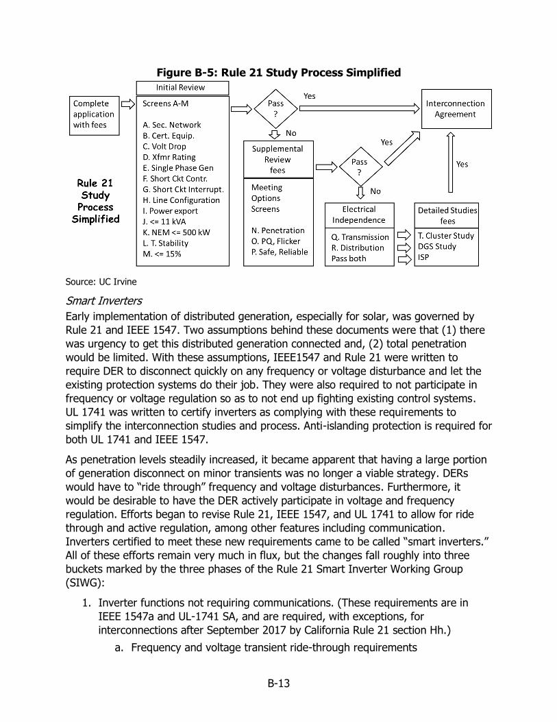
B-13
Figure B-5: Rule 21 Study Process Simplified
Source: UC Irvine
Smart Inverters
Early implementation of distributed generation, especially for solar, was governed by
Rule 21 and IEEE 1547. Two assumptions behind these documents were that (1) there
was urgency to get this distributed generation connected and, (2) total penetration
would be limited. With these assumptions, IEEE1547 and Rule 21 were written to
require DER to disconnect quickly on any frequency or voltage disturbance and let the
existing protection systems do their job. They were also required to not participate in
frequency or voltage regulation so as to not end up fighting existing control systems.
UL 1741 was written to certify inverters as complying with these requirements to
simplify the interconnection studies and process. Anti-islanding protection is required for
both UL 1741 and IEEE 1547.
As penetration levels steadily increased, it became apparent that having a large portion
of generation disconnect on minor transients was no longer a viable strategy. DERs
would have to “ride through” frequency and voltage disturbances. Furthermore, it
would be desirable to have the DER actively participate in voltage and frequency
regulation. Efforts began to revise Rule 21, IEEE 1547, and UL 1741 to allow for ride
through and active regulation, among other features including communication.
Inverters certified to meet these new requirements came to be called “smart inverters.”
All of these efforts remain very much in flux, but the changes fall roughly into three
buckets marked by the three phases of the Rule 21 Smart Inverter Working Group
(SIWG):
1. Inverter functions not requiring communications. (These requirements are in
IEEE 1547a and UL-1741 SA, and are required, with exceptions, for
interconnections after September 2017 by California Rule 21 section Hh.)
a. Frequency and voltage transient ride-through requirements

B-14
b. Active voltage regulation
2. Communications for smart inverters
a. Expected to require compliance with IEEE 2030.5 (Smart Energy 2.0
protocol)
3. Inverter functions requiring communications (These are the subject of a full
revision of IEEE 1547 and further revision of Rule 21, both are in progress
a. Monitor key DER data
b. Disconnect and reconnect
c. Active power limitations
d. Frequency Watt regulation
e. Volt Watt regulation
f. Volt-var regulation
g. Scheduling
Electricity Market Fundamentals The ideal objective of deregulation is to achieve lower costs due to competition
introduced by markets. However, electricity is different from other commodities (such
as natural gas) because of its physical characteristics that require supply and demand
match at each point and instant in the system in the absence of economically viable
massive energy storage and considering that even with demand response programs,
electricity demand is still quite rigid and does not respond to price signals like other
commodities. Thus in practice, the demand curve is largely inelastic. Buyers need a
certain amount of electricity for their customers and in the short term at least will
accept a wide range of prices. Furthermore, retail consumers of electricity lack
information and control to respond to short term changes in price, a condition smart
meters and smart grid technology is trying to remedy. Better demand response to price
is widely seen as important to the satisfactory functioning of the electricity market.
Energy market is where the competitive trading of electricity occurs. Those who wish to
buy or sell power (SCs in the case of the CAISO) submit their bids one day ahead of the
actual dispatch into a day-ahead market. Previously, the intersection of the supply and
demand curves was declared as the market clearing price (MCP). With the inclusion of
congestion, an adjustment would be done to the price in the form of congestion or
capacity charge. In a restructured market, the ISO uses a security-constrained unit
commitment (SCUC) to clear the day-ahead energy market. The objective of this market
is to maximize social welfare while complying with all the physical constraints of the
system. In a day-ahead energy market, the bid-in supply is cleared against the bid-in
demand. Those generating units cleared, are then committed to participate in the real-
time market (thus the term unit commitment). In the real-time market, the ISO makes

B-15
sure that there is enough supply to meet the demand and if not it uses ancillary
services to procure more energy.
In some markets, generators are allowed to enter a single bid, while in others such as
the CAISO, a multi-bid approach is used which include start-up, minimum load, and
energy bids. These energy bids are shown in Figure B-6.
Figure B-6: Energy Bids (a) Multipart (b) Single-part
Source: UC Irvine
To ensure supply and demand balance and the reliability of the system, the ISO needs
to procure ancillary services. In a deregulated market, however, the ancillary services
are procured by the ISO through a competitive market. There are two approaches for
settling ancillary services markets: sequential approach, and simultaneous approach. In
the sequential approach, the market is cleared for the highest quality service first, then
the next highest, and so on until all the reliability requirements are met. The alternative
is to clear all ancillary services simultaneously by introducing a rational buyer. In a
rational buyer auction, all the ancillary services are cleared together and the
substitution of lower quality services with higher quality ones, is done automatically by
the ISO.
There are also several methods to pay the cleared generators. One way is to pay them
what they had bid in, pay as bid pricing. The other option is to pay everyone a uniform
price witch is known as uniform pricing. In uniform pricing, all providers are paid the
market clearing price. In ancillary services markets, there are various options for
uniform pricing: marginal pricing, demand substitution, and supply substitution pricing.
In marginal pricing, the marginal cost of a service is chosen as its price. In demand
substitution pricing, the demand for a lower quality service can be substituted by a
higher quality service and the price is set to the highest accepted bid for that service. In

B-16
a supply substitution pricing, the supply for a higher quality service can be used for a
lower quality service and the price is set to the highest accepted bid of that service59.
CAISO Markets Overview
Between 1998 and 2001, the CAISO did not allow bilateral contracts by Investor Owned
Utilities (IOU) and the majority of the load had to go through the forward spot market
which was run by CalPX (California Power Exchange). After the crisis and CalPX being
out of business, it was clear that bilateral forward contracts must be allowed to
minimize exposure to spot market prices. Today, the majority of the electricity demand
in California is served through long-term bilateral contracts. The CPUC requires all LSEs
to procure enough capacity to meet 115% of their forecast load. LSEs meet 80-90% of
their projected load by means of bilateral contracts with energy suppliers via
competitive RFPs. This procurement process has to be open and possibly overseen by a
neutral third party monitor. These contracts are for both energy and capacity and
consider both economic and non-economic factors. Capacity purchases are based on
the supplier’s Net Qualifying Capacity (NQC) which considers transmission deliverability
and performance track record. The remaining energy and capacity is purchased on the
CAISO market in a two-step process consisting of a Day ahead Market (DAM) and a
Real Time Market (RTM).
Prior to Market Redesign and Technology Upgrade (MRTU) in April 2009, CAISO
balancing area was separated into three zones and the network model used these three
zones for market clearing and managing congestion. After MRTU, CAISO adopted a
nodal system in which the full network model is solved and the transmission constraints
are solved between various nodes on the system. In this new approach, there is no
distinction between inter- and intra-zonal congestions, but the competitive and non-
competitive paths are distinguished from one another in order to mitigate the local
market power, and also provide incentives to invest in congested paths. This distinction
is done through introducing the Locational Marginal Pricing (LMP) at each node of the
system instead of the previously used zonal pricing.
In DAMs energy, ancillary services, congestion and losses are optimized simultaneously
as Integrated Forward Market (IFM), all in one single optimization. After all bids are
submitted, and before running the IFM, the CAISO performs a Reliability Requirement
Determination and Local Market Power Mitigation in order to validate the bids and make
sure that none of the parties are exercising market power and if they are, they will be
subject to a bid adjustment. After the IFM, the CAISO performs a reliability run. The
generators that have not been cleared in the IFM, are then eligible to participate in the
59 Razeghi, G. The Development and Evaluation of a Highly-Resolved California Electricity Market Model to
Characterize the Temporal and Spatial Grid, Environmental, and Economic Impacts of Electric Vehicles.
Ph.D. Dissertation. University of California, Irvine. 2013

B-17
Residual Unit Commitment (RUC). The RUC is performed to match the generation with
the CAISO forecast of the next day’s demand to ensure reliability.
Real-time market (RTM) includes several processed such as Short Term Unit
Commitment (STUC) to commit units with medium or short startup requirements, Hour-
Ahead Scheduling Process (HASP) which results in an advisory schedule for P-Nodes
and firm schedule for import/export to CAISO, Real-time Unit Commitment (RTUC)
every fifteen minutes, Security-Constrained Economic Dispatch (SCED) on a five-minute
basis, and Real-Time Contingency Dispatch and Exceptional (Manual) Dispatch in case
of contingencies and unforeseen occurrences. The details of these processes as well as
Full Network Model (FNM) can be found in various CAISO documents and websites
some provided in the References section.