statics and dynamics simulation of a multi- tethered...
TRANSCRIPT

Statics and Dynamics Simulation of a Multi-
Tethered Aerostat System by
Xiaohua Zhao B.Sc., Nanjing University of Aeronautics & Astronautics, 1994
A Thesis Submitted in Partial Fulfillment of the
Requirements for the Degree of
MASTER OF APPLIED SCIENCE
in the Department of Mechanical Engineering
We accept this thesis as conforming
to the required standard
Dr. M. Nahon, Supervisor (Dept. of Mechanical Engineering)
Dr. Z. Dong, Departmental Member (Dept. of Mechanical Engineering)
Dr. B. Buckham, Departmental Member (Dept. of Mechanical Engineering)
Dr. W.-S. Lu, External Member (Dept. of Electrical & Computer Engineering)
© Xiaohua Zhao, 2004
University of Victoria
All right reserved. This thesis may not be reproduced in whole or in part, by photocopy or
other means, without the permission of the author.

ii
Supervisor: Dr. M. Nahon
Abstract
A new radio telescope composed of an array of antennas is under development at
the National Research Council. Each antenna includes a large scale multi-tethered
aerostat system to hold the telescope receiver at the reflector focus. This receiver is
located at the confluence point of the tethers.
Starting from a previously developed dynamics simulation of the triple-tethered
aerostat system, an existing statics model of the same system is incorporated into the
simulation to provide an initial equilibrium condition for the dynamics. A spherical
aerostat is used in both models. The two models show a very good match with each other
after being merged together. This combined computer model is further developed to
study the use of six tethers and the use of a streamlined aerostat instead of a spherical one.
In the case of the six-tethered system, two topics were investigated: using the six tethers
to control the position of the airborne receiver only; and using the six tethers to control
the orientation of the receiver as well as its position. A streamlined aerostat is also
modelled by a component breakdown method and incorporated into the triple-tethered
system to replace the spherical one.
The main findings from the simulation results are as follows: (1) the six-tethered
system with reductions in the tether base radius and the tether diameter exhibited
increased stiffness compared to the triple-tethered system when used to control the
receiver position only; (2) the six-tethered system showed difficulty achieving

iii
satisfactory control for both the position and orientation of the receiver; (3) the
streamlined aerostat showed no oscillations typical of a spherical one but the system
requires more power to control in the presence of wind turbulence.
Examiners:
Dr. M. Nahon, Supervisor (Dept. of Mechanical Engineering)
Dr. Z. Dong, Departmental Member (Dept. of Mechanical Engineering)
Dr. B. Buckham, Departmental Member (Dept. of Mechanical Engineering)
Dr. W.-S. Lu, External Member (Dept. of Electrical & Computer Engineering)

iv
Table of Contents
Abstract ………………………………………………………………………………… ii
Table of Contents ............................................................................................................. iv
List of Tables ................................................................................................................... vii
List of Figures................................................................................................................. viii
Acknowledgements ............................................................................................................x
Dedication……………………………………………………………………………… xii
Chapter 1 Introduction................................................................................................... 1
1.1 Background ......................................................................................................... 1
1.2 Related Work ...................................................................................................... 5
1.3 Research Focus ................................................................................................... 8
Chapter 2 Kinematics ................................................................................................... 10
2.1 Reference Frames.............................................................................................. 10
2.2 Translational Kinematics .................................................................................. 12
2.3 Orientations and Rotational Transformations................................................... 13
2.3.1 The Z-Y-X Euler Angle Set and its Transformations ................................ 14
2.3.2 The Z-Y-Z Euler Angle Set and its Transformations ................................ 16
Chapter 3 Statics ........................................................................................................... 18
3.1 Model Overview and Problem Description ...................................................... 18
3.1.1 The Aerostat Model .................................................................................. 19
3.1.2 The Payload Platform Model .................................................................... 20
3.1.3 The Cable Model....................................................................................... 20
3.2 Fitzsimmons’ Statics Solution .......................................................................... 22
3.3 Implementation and Modifications of Fitzsimmons’ Solution ......................... 36
3.4 Verification of the Statics Model...................................................................... 38

v
Chapter 4 Six-Tethered System ................................................................................... 42
4.1 Dynamics of the Triple-Tethered System......................................................... 42
4.2 Redundantly Actuated System.......................................................................... 47
4.2.1 Actuation Redundancy.............................................................................. 48
4.2.2 Redundancy in Statics............................................................................... 49
4.2.3 Constrained Optimization Problem........................................................... 50
4.2.4 Nonlinear Optimizer CFSQP .................................................................... 50
4.2.5 Implementation in the Statics.................................................................... 52
4.2.6 Dynamics of the Six-Tethered System ..................................................... 55
4.2.7 Statics Results and Verification ................................................................ 55
4.2.8 Optimization Results and Discussion ....................................................... 57
4.2.9 Dynamics Results and Discussion ............................................................ 64
4.3 Determinate System.......................................................................................... 68
4.3.1 Purpose...................................................................................................... 69
4.3.2 The 6-DOF Payload Platform Model........................................................ 69
4.3.2.1 Statics.................................................................................................... 70
4.3.2.2 Dynamics .............................................................................................. 71
4.3.3 Results and Discussion ............................................................................. 74
Chapter 5 Incorporation of a Streamlined Aerostat.................................................. 83
5.1 Vehicle Introduction ......................................................................................... 83
5.2 Modelling the TCOM 71M Aerostat ................................................................ 86
5.2.1 Reference Frames...................................................................................... 87
5.2.2 Scaled Parameters ..................................................................................... 88
5.2.2.1 Moments and Products of Inertia.......................................................... 89
5.2.2.2 The Center of Mass............................................................................... 91
5.2.2.3 The Leash Attachment Point................................................................. 91
5.2.3 Estimated Center of Buoyancy ................................................................. 92
5.2.4 Aerostat Component Breakdown.............................................................. 93
5.2.4.1 The Hull ................................................................................................ 93
5.2.4.2 The Fins ................................................................................................ 97

vi
5.2.4.3 The Bulge.............................................................................................. 98
5.2.5 Added Mass and Moments........................................................................ 99
5.3 Model Validation ............................................................................................ 101
5.4 Implementation and Incorporation.................................................................. 103
5.4.1 Statics...................................................................................................... 104
5.4.2 Dynamics ................................................................................................ 106
5.5 Results & Discussions..................................................................................... 108
Chapter 6 Conclusions................................................................................................ 116
6.1 Conclusions..................................................................................................... 116
6.2 Future Work .................................................................................................... 118
Bibliography …………………………………………………………………………..121

vii
List of Tables
Table 3.1 Spherical aerostat properties............................................................................ 19
Table 3.2 Cable properties ............................................................................................... 21
Table 3.3 Conditions of simulation cases ......................................................................... 39
Table 4.1 Parameter changes ............................................................................................ 55
Table 4.2 Objective functions for no-wind analysis ........................................................ 57
Table 4.3 Case number definitions for Figure 4.7 ........................................................... 61
Table 4.4 Payload position errors for the redundantly actuated system .......................... 65
Table 4.5 Simulation conditions ....................................................................................... 74
Table 5.1 The TCOM 71M aerostat parameters [17], [36].............................................. 85
Table 5.2 Balloon properties [39] .................................................................................... 88
Table 5.3 Ratios between the two vehicles...................................................................... 90
Table 5.4 Moments and product of inertia....................................................................... 90
Table 5.5 Parameters of the fins and the bulge................................................................ 99
Table 5.6 Aerostat pitch angles under different conditions ........................................... 105
Table 5.7 Payload position errors .................................................................................. 109

viii
List of Figures
Figure 1.1 An example of present-day steerable telescope................................................. 2
Figure 1.2 LAR Portrait View [5]...................................................................................... 3
Figure 1.3 LAR Concept [7] .............................................................................................. 4
Figure 2.1 Reference frames ............................................................................................. 11
Figure 2.2 The body-fixed frame for a streamlined aerostat ........................................... 12
Figure 2.3 Z-Y-X Euler Angles [25]................................................................................. 14
Figure 3.1 Cable segment model (statics)......................................................................... 21
Figure 3.2 Flowchart of statics solution by Fitzsimmons ................................................ 24
Figure 3.3 The strained cable profile ............................................................................... 25
Figure 3.4 Tethers in a 3-D space .................................................................................... 27
Figure 3.5 Tether segment analysis ................................................................................. 29
Figure 3.6 Tether profile calculation (Block D in Figure 3.2)......................................... 30
Figure 3.7 Approximation used in tether analysis ............................................................ 32
Figure 3.8 Leash analysis................................................................................................. 33
Figure 3.9 Wind models................................................................................................... 37
Figure 3.10 Errors of the CP when using statics solution as the initial states ................. 40
Figure 4.1 Cable segment model (dynamics) .................................................................. 43
Figure 4.2 The tethered aerostat system model in 2-D [24] ............................................ 44
Figure 4.3 Controller 2-D illustration [24] ...................................................................... 46
Figure 4.4 Matching simulations for the six-tethered spherical aerostat system............. 56
Figure 4.5 Tether tensions in statics using different objective functions ........................ 59
Figure 4.6 Results for different objective functions, θza = θza = 0................................... 60
Figure 4.7 Dynamics simulation results of the payload position using different objective
functions for the statics initial condition................................................................... 62
Figure 4.8 Dynamics simulation results of the tether tensions using different objective
functions for the statics initial condition................................................................... 63
Figure 4.9 Payload motion for θza = θaz = 0..................................................................... 66

ix
Figure 4.10 Tether tension forθza = θaz = 0 ..................................................................... 66
Figure 4.11 Playload motion for θza = 60°, θaz = 0 .......................................................... 67
Figure 4.12 Tether tension for θza = 60°, θaz = 0 ............................................................. 67
Figure 4.13 The Airborne platform view [5] ................................................................... 68
Figure 4.14 2-D illustration of the winch controller ........................................................ 73
Figure 4.15 Payload platform orientation ........................................................................ 76
Figure 4.16 Payload position error.................................................................................. 77
Figure 4.17 Tether tensions.............................................................................................. 79
Figure 4.18 Top view of the six-Tether configuration..................................................... 80
Figure 5.1 The TCOM 71M aerostat [35]........................................................................ 84
Figure 5.2 The structure of the TCOM 71M aerostat ...................................................... 87
Figure 5.3 Reference frames of the aerostat .................................................................... 87
Figure 5.4 Tethered balloon layout [39] .......................................................................... 89
Figure 5.5 Modelling the hull .......................................................................................... 94
Figure 5.6 Center of pressure of the hull ......................................................................... 96
Figure 5.7 Center of pressure of the fin ........................................................................... 98
Figure 5.8 Normal force coefficient and pitching moment coefficient about the nose of
the TCOM 71M....................................................................................................... 102
Figure 5.9 Aerodynamic model of [36] compared with wind tunnel data [36] ............. 103
Figure 5.10 External forces applied to the aerostat........................................................ 107
Figure 5.11 Aerostat translational motion for θza = θaz = 0 .......................................... 110
Figure 5.12 Aerostat rotational motion for θza = θaz = 0............................................... 110
Figure 5.13 Payload position error for θza = θaz = 0 ..................................................... 111
Figure 5.14 Tether tensions for θza = θaz = 0 ................................................................ 111
Figure 5.15 Aerostat translational motion for θza = 60°, θaz = 0.................................... 112
Figure 5.16 Aerostat rotational motion for θza = 60°, θaz = 0 ......................................... 112
Figure 5.17 Payload position error for θza = 60°, θaz = 0............................................... 113
Figure 5.18 Winch tensions for θza = 60°, θaz = 0.......................................................... 113

x
Acknowledgements
I would like to thank many people who helped me fulfill my M.A.Sc. study. First,
and above all, Dr. Meyer Nahon for his enthusiastic and extraordinary supervision and
guidance during these years. I have learnt a great deal from him. I would also express my
heartfelt gratitude to Dr. Zuomin Dong, Dr. Brad Buckham and Dr. Wu-Sheng Lu for
being in my thesis committee and offering their observations and suggestions. Their
efforts added new insights into my work. I would like to extend my sincere appreciation
to Dr. Joeleff Fitzsimmons for his contribution to my work.
I am very grateful to Prof. Yuncheng Xia, Prof. Yongzhang Shen, Prof. Daiye Lin
and Prof. Zhenqiu Yang. Not only did they teach me academic knowledge during my
years in Nanjing, but also taught me to be a better person by their own examples, and
gave me fatherly moral support ever since I lost my father in 1998.
I would also like to thank Juan Carretero, Gabriele Gilardi, Casey Lambert, Sheng
Wan, Rong Zheng, Xiang Diao, Lu Liu and Ruolong Ma, Andy Yu and Kevin Deane-
Freeman for sharing their knowledge and helping on many occasions. Thanks to Lei
Hong, Nina Ni, Huiyan Zhou, Juan Liu, Shaun Georges and Richard Barazzuol for
cheering me on and helping me get through hard times. Special thanks to Manjinder
Mann for his immense patience and support.
I am forever indebted to my parents. My father, Chuanyuan Zhao, had always
encouraged and fully supported me. I will always have him in my heart. As well, my
mother has always been extremely patient and supportive in all my endeavors. Their love

xi
has always been the greatest inspiration for me. I am also thankful to my brother Bo and
sister Xiaoyu for their constant support.
Apart from the people mentioned above, many others have helped along the way.
I cannot name all here, but I remain indebted to them.
My deep thanks to all for making my life so much fuller!

xii
Dedication
To those who have loved me so much…

Chapter 1 Introduction
1.1 Background
The latest developments in astronomy have motivated astronomers worldwide to
plan for the next generation of radio telescopes. It is now believed that a new radio
telescope with unprecedented sensitivity will be needed to study the earliest universe.
This proposed revolutionary radio telescope will have an effective collecting area of one
million square metres, much greater than that of the largest radio telescope in service.
The astronomy community around the globe has aimed to build such a radio telescope in
the next decade. This international project is known as the Square Kilometre Array (SKA)
[1]. A Memorandum of Agreement on this international SKA project has been signed by
a number of organizations from several countries including Australia, Canada, China,
India, the Netherlands, and the U.S.A. [2].
The SKA will consist of an array of stations, spread over an area one thousand
kilometres in diameter. Each station of the array will be a telescope in its own right, with
an aperture up to 200 metres.
The size of each telescope will be much larger than the present-day fully steerable
radio telescopes (Figure 1.1 shows the 25 m dishes of the Very Large Array in New

2
Mexico [3]). For this reason, it would not be cost effective to build the Square Kilometre
Array with conventional technology. A new means must be established to construct a
very large aperture radio telescope like this. Research and development activities are
ongoing at several international centres. In Canada, the Large Adaptive Reflector (LAR)
approach is under study as a solution [4]. This development work is funded by National
Research Council, Canada (NRCC), and coordinated by Dominion Radio Astrophysical
Observatory (DRAO) with collaborators in universities and industry [5].
Figure 1.1 An example of present-day steerable telescope (The Very Large Array of fully steerable telescopes in New Mexico [3])
The LAR, proposed by Legg of NRCC’s Herzberg Institute of Astrophysics
(HIA) and shown diagrammatically in Figure 1.2, is a long focal-length (about 500
metres), large diameter (about 200 metres) parabolic reflector which requires an airborne
platform to support the focal receiver [4]. An array of about 50 LARs would be used to
build the SKA. The reflector is composed of many flat panels, which are supported by the

3
ground. The shape of the reflecting surface can be adjusted by actuators under the panels.
Steering is realized by adjusting the shape of the reflector and the position of the airborne
platform where the receiver feed is located. A key challenge to implement the LAR
design is to accurately control the position of the airborne platform. This subsystem is the
focus of this thesis. The receiver’s position will be controlled by three or more cables and
winches, and an aerostat will be used to provide lifting force for the system.
Figure 1.2 LAR Portrait View [5]
Using tensioned cables to support the airborne platform places this system in a
class of structures known as tension structures. The advantages of such a system include
[6]:
1) The structure has a high ratio of payload to structural weight;

4
2) The cables are highly tensioned by the aerostat lift at static equilibrium. This
stiffens the structure, reduces deflection due to perturbations, and stabilizes
the structure;
3) The structure is easily reconfigurable by changing the cable lengths;
4) The environmental loads are efficiently carried by direct tensile stress,
without bending.
Figure 1.3 LAR Concept [7]
Figure 1.3 shows the geometry of the LAR. The airborne platform will be at the
focus of the reflector. The focal plane is the ∆za-∆az plane. θza is the zenith angle of the
airborne platform, and θaz is its azimuth angle. R is the distance from the center of

5
reflector to the focus, and would vary with zenith and azimuth angles. This study focuses
on the performance of the system with a goal of keeping the airborne platform positioned
on the surface of a hemisphere of constant radius R = 500 m. Figure 1.2 illustrates the
portrait view of such a radio telescope antenna system with six tethers and a spherical
aerostat.
A computer simulation of this system will be presented to study the statics and
dynamics of the system. Considering the scale of the system, a computer simulation is an
inexpensive and valuable tool to perform preliminary study of the system when compared
to building prototypes. It can provide good insight into the behaviour of the system and
help with the system design.
1.2 Related Work
Analysing this novel multi-tethered system requires a consideration of the statics
and dynamics of cables and aerostats. Cable structures are considered to be difficult to
analyze because of their nonlinear behaviour. For most realistic problems, it is typically
not considered practical to obtain statics, dynamics and displacement solutions using a
continuous cable model. For this reason the cables are usually analysed numerically using
discrete models such as lumped mass or rod models. A rod model consists of rods
connected by frictionless hinges at the endpoints to form a chain [8]. A lumped mass
model, originally proposed by Walton and Polacheck [9], consists of point masses
connected by weightless rigid or flexible links [9] [10] [11] [12]. Forces acting on each
rod or segment are applied at the endpoints to set up motions equations in three-
dimension. The motion of the system is obtained by integrating the motion equations.
6
Both modelling methods are widely used in study of cable systems. Sanders [8] showed a
finite difference formulation to develop the discretized equations of motion for a towed
system. Kamman et al. [10], [12], and Buckham, et al. [11] employed lumped mass or
lumped parameter models in their simulation of towed cable systems. These results
showed simulation results that were qualitatively and quantitatively reasonable. Lumped
mass modelling is the method used in this work.
Since the decision of whether to use a streamlined or spherical aerostat for LAR
has not yet been finalized, both types of aerostats are studied in this work. The dynamics
of a spherical aerostat are straightforward because of its uniform shape. It is more
difficult to analyze the dynamics characteristics of a streamlined aerostat.
The analysis of the dynamics of aerostats and airships requires knowledge of
aerodynamic forces and moments applied on an aerostat or airship. Aerodynamic forces
and moments of the hull of an aerostat or airship can be calculated based on its geometry
and flow characteristics [13]. This method of analysis was developed by Allen and
Perkins [14] from Munk’s normal-force and potential-flow equations for airship bodies
[15]. Jones and DeLaurier based their estimation techniques of aerostats and airships'
aerodynamic properties [13] on a semiempirical airship model that included a
consideration of the hull-fin mutual interference factors and added mass for greater
accuracy.
Tethered aerostat systems have received limited attention. Previous studies have
been concerned mainly with single-tethered systems. Jones and Schroeder presented
some dynamic simulations of tethered/moored streamlined aerostat system [16], [17],
[18], which were mainly focused on the verification of aerodynamic characteristics of the

7
streamlined aerostat model, with no discussion of the tether’s dynamics or closed loop
control of the tethered system.
Some work was performed in the early 70’s by the US Air Force, comparing a
multi-tethered aerostat system to a single tethered arrangement [19], [20]. They found the
multi-tethered system greatly reduced the motion dispersions of the system.
Some investigations have been carried out during the past a few years on tethered
spheres. Results demonstrate that a tethered sphere will oscillate strongly at a saturation
amplitude of close to two diameters peak-to-peak in a steady fluid flow. The oscillations
induce an increase in drag and tether angle on the order of around 100% over what is
predicted using steady drag measurements. The in-line oscillations vibrate at twice the
frequency of the transverse motion [21], [22].
In Canada, scientists and engineers from research institutes, universities and
industry are working together to develop the LAR concept. Veidt, Dewdney, and
Fitzsimmons of NRCC’s HIA, worked on the steady-state stability analysis of the multi-
tethered LAR aerostat platform [7], [23]. Their steady-state analysis results showed that
this tethered aerostat system will operate reliably in moderate weather condition. Nahon
later performed a dynamics simulation of the triple-tethered spherical aerostat system
[24]. The numerical simulation results presented there indicate that the spherical aerostat
system can be accurately controlled in the presence of disturbances due to turbulence.
These encouraging results have led to this work, which is a further study of the multi-
tethered aerostat system. It is worth noting that Fitzsimmons’ work is used as the basis
for the initial determination of equilibrium state in this study. Detailed descriptions of this

8
will be given in Chapter 3. As well, Nahon’s work is used as the basis for the dynamics
work in this study, and this will be further discussed in Chapter 4.
1.3 Research Focus
The studies presented in this work are intended to provide preliminary insight into
the LAR system, and thus help the design of the system.
The specific topics covered are an analysis of the six-tethered system with a
spherical aerostat and triple-tethered system with a streamlined aerostat. In the six-
tethered system case, two operational modes are studied: redundantly-actuated and
determinate. In the redundantly-actuated mode, the six main tethers are used to control
the payload position only; in the determinate mode, the six tethers are used to control
both the position and orientation of the payload platform. Statics analyses are used to
provide initial states for the dynamics simulation. Dynamics simulations are carried out
for different system configurations.
Studying the dynamics of this complex system involves transforming quantities of
interest between different reference frames. Chapter 2 explains the relationship between
frames and describes the transformations used in this work.
Chapter 3 discusses the statics analysis adopted from Fitzsimmons and the changes
made to it in order to be incorporated into the dynamics work.
The six-tethered system is covered in Chapter 4. We first introduce Nahon’s
dynamics model of the triple-tethered system with a spherical aerostat. Then the
redundantly-actuated six-tethered system is discussed and a variety of objective functions
are evaluated to solve the underdetermined statics problem. Dynamics simulation results

9
are presented as well. In addition, we study the determinate six-tethered system in which
the position and orientation of the payload platform are controlled by changing the length
of the tethers. Some results are shown to illustrate the findings. It is worth mentioning
that the vortex-induced oscillations typical of the spherical aerostat are not included in
the spherical aerostat model.
In Chapter 5, we deal with the incorporation of a streamlined aerostat to replace the
spherical one in the triple-tethered system. Modelling of the streamlined aerostat is
covered and validation results are presented. Simulation results are then discussed.
Finally, Chapter 6 gives an overview the work accomplished. Conclusions and
recommendations for future work are presented there.

10
Chapter 2 Kinematics
When formulating mechanics problems, a number of reference frames must be used
to specify relative positions and velocities, components of vectors (e.g. forces, velocities,
accelerations). As well, formulae for transforming quantities of interest from one frame to
another must be available.
2.1 Reference Frames
An inertial reference frame is essential to dynamic problems, while other frames are
usually also defined for the convenience of the problem at hand. In this study, the
reference frames include an inertial frame and a number of body-fixed frames. All frames
used are right-handed.
The inertial reference frame, OIXIYIZI, shown in Figure 2.1, is fixed to the ground
with its origin OI at the center of the reflector, and OIZI directed vertically up. OIXIYI
defines the horizontal plane, with OIXI pointing to the base of the first tether and OIYI
defined to complete a right-handed coordinate system.
The body-fixed frames are defined to describe motions of bodies such as tether
elements, the payload platform, and the aerostat in the system. Figure 2.1 illustrates

11
body-fixed frames for various moving bodies. Frame OtiXtiYtiZti is attached to tether
element i, while frame OaXaYaZa moves with the aerostat, and frame OpXpYpZp is
embedded in the payload platform.
Figure 2.1 Reference frames
Frame OtiXtiYtiZti is the body-fixed frame for tether i element, where i = 1, …, nt
where nt is the total number of tether elements. Oti is located at the lower end of the
element, axes OtiXti and OtiYti are the local normal and binormal direction, and axis OtiZti
is tangent to the element.
Frame OaXaYaZa, when used with a spherical aerostat, is defined such that when the
aerostat is in its equilibrium condition directly above the center of reflector OI, the axes
XI
ZI
YI
OI
Tether number increases
Tether #1
Reflector
Tether #2
Tether #3
Xp
Yp Zp
Op
Oti Xti
Yti Zti
Za
Ya
Aerostat
Payload
Xa

12
OaXa, OaYa and OaZa are aligned with those of the inertial frame.
When a streamlined aerostat is used, the body-fixed frame is defined as shown in
Figure 2.2, with its origin at the center of mass of the aerostat. The Xa-axis points forward,
the Ya-axis points left and the Za-axis points upwards. Also shown in Figure 2.2 are the
components of the aerostat’s angular velocity p, q, r.
Figure 2.2 The body-fixed frame for a streamlined aerostat
The payload platform’s body-fixed frame OpXpYpZp has its origin at the center of
mass, OpZp is directed upwards and perpendicular to the disk plane OpXpYp. Axes OpXp
and OpYp are aligned with OIXI and OIYI respectively, when the disk is in its equilibrium
configuration above the center of reflector as shown in Figure 2.1.
2.2 Translational Kinematics
The position of an object is usually expressed in terms of the relation of a particular
reference point on the object to the origin of a reference frame. For example, the position
of the payload platform is expressed by the position vector of its center of mass with
⊗
Za Ya
Xa
p
qr
Oa

13
respect to the origin of the inertial frame OIXIYIZI (Figure 2.1), and expressed as
components in the inertial frame, i.e.,
⎥⎥⎥
⎦
⎤
⎢⎢⎢
⎣
⎡
=
zI
yI
xI
I
rrr
r
Similarly, position vectors expressed in the inertial frame are used to denote the positions
of the aerostat, and all the cable nodes. In some cases, it is more convenient to express the
position of an object in a local body-fixed frame. For example, the position of the above-
mentioned point on the payload platform may be expressed in the aerostat body-fixed
frame as
⎥⎥⎥
⎦
⎤
⎢⎢⎢
⎣
⎡
=
zB
yB
xB
B
rrr
r
The leading superscript ‘B’ stands for the Body-fixed frame.
The translational velocities can be naturally expressed by the time derivatives of
position vectors. As well, the translational accelerations would be represented by second
time derivatives of the position vectors.
2.3 Orientations and Rotational Transformations
The orientation of one reference frame with respect to another can be represented
using Euler angles. For convenience, two sets of angles, Z-Y-X and Z-Y-Z Euler angles
[25], are chosen to describe the orientations. The orientation of the body-fixed frame of
the payload platform is represented by a set of Z-Y-Z Euler angles. In all other cases, a Z-
Y-X Euler angle set is used.

14
2.3.1 The Z-Y-X Euler Angle Set and its Transformations
The Z-Y-X Euler angles describing the orientation of a body-fixed frame with respect
to the inertial frame are obtained by the following three rotations (Figure 2.3), starting
with a frame coincident with the inertial frame:
1) A rotation by ψ about the Z-axis;
2) A rotation by θ about the Y-axis which results from the previous rotation;
3) A rotation by φ about the X-axis resulting from the last rotation.
Figure 2.3 Z-Y-X Euler Angles [25]
The resulting rotation matrix which maps vector components in the body-fixed frame
to components in the inertial frame is as follows:
⎥⎥⎥
⎦
⎤
⎢⎢⎢
⎣
⎡
−−++−
=θφθφθ
ψφψθφψφψθφψθψφψθφψφψθφψθ
coscoscossinsincossinsinsincoscoscossinsinsinsincossinsincossincossincoscossinsincoscos
ZYXIBT (2.1)
A feature of rotation matrices is that they are orthogonal, and the inverse is therefore

15
simply given by the transpose.
TZYX
IBZYX
BI TT =−1
When applied to the tether element local frame, the Euler angle ψ is set to zero since
the torsion of the tether is not considered in the tether model. We then get a simpler form
of the rotation matrix
⎥⎥⎥
⎦
⎤
⎢⎢⎢
⎣
⎡
−−−=
θφθφθφφ
θφθφθ
coscoscossinsinsincos0
sincossinsincos
ZYXIBT (2.2)
Transformations between the angular velocities p, q, r (see Figure 2.2) and time
derivatives of Euler anglesθ& , φ& and ψ& are necessary for the dynamics analysis. When
employing a Z-Y-X Euler angle set, the kinematic relations are:
φ& = p + (sinφ tanθ ) q + (cosφ tanθ) r
θ& = (cosφ) q – (sinφ) r
ψ& = (sinφ secθ ) q + (cosφ secθ) r
Or, in matrix form
⎥⎥⎥
⎦
⎤
⎢⎢⎢
⎣
⎡
⎥⎥⎥
⎦
⎤
⎢⎢⎢
⎣
⎡−=
⎥⎥⎥
⎦
⎤
⎢⎢⎢
⎣
⎡
rqp
θφθφφφ
θφθφ
ψθφ
cos/coscos/sin0sincos0
tancostansin1
&
&
&
(2.3)
Based on this transformation matrix, we see that this Euler angle set becomes
degenerate when θ = 90°. However, this condition is never reached in our simulations.
It should be noted that this transformation is not orthogonal. The corresponding
inverse transformation is as follows:

16
⎥⎥⎥
⎦
⎤
⎢⎢⎢
⎣
⎡
⎥⎥⎥
⎦
⎤
⎢⎢⎢
⎣
⎡
−
−=
⎥⎥⎥
⎦
⎤
⎢⎢⎢
⎣
⎡
ψθφ
φθφφθφ
θ
&
&
&
coscossin0sincoscos0
sin01
rqp
(2.4)
2.3.2 The Z-Y-Z Euler Angle Set and its Transformations
The Z-Y-Z Euler angles are obtained by the following three rotations, starting with a
frame coincident with the inertial frame:
1) A rotation by α about the Z-axis;
2) A rotation by β about the Y-axis which results from the previous rotation;
3) A rotation by γ about the Z-axis resulting from the last rotation.
The resulting rotation matrix which maps vector components in the body-fixed frame
to components in the inertial frame is as follows:
⎥⎥⎥
⎦
⎤
⎢⎢⎢
⎣
⎡
−+−+−−−
=βγβγβ
βαγαγβαγαγβαβαγαγβαγαγβα
cossinsincossinsinsincoscossincossinsincoscoscossinsincoscossinsincoscossinsincoscoscos
ZYZIBT
(2.5)
The transformations between the angular velocities in the body-fixed frame and the
time derivative of Euler angles are as follows:
⎥⎥⎥
⎦
⎤
⎢⎢⎢
⎣
⎡
⎥⎥⎥
⎦
⎤
⎢⎢⎢
⎣
⎡
−
−=
⎥⎥⎥
⎦
⎤
⎢⎢⎢
⎣
⎡
rqp
1tan/sintan/cos0cossin0sin/sinsin/cos
βγβγγγ
βγβγ
γβ
α
&
&
&
(2.6)
and

17
⎥⎥⎥
⎦
⎤
⎢⎢⎢
⎣
⎡
⎥⎥⎥
⎦
⎤
⎢⎢⎢
⎣
⎡−=
⎥⎥⎥
⎦
⎤
⎢⎢⎢
⎣
⎡
γβ
α
βγβ
γγβ
&
&
&
10cos0cossinsin0sincossin
γrqp
(2.7)
The Z-Y-Z Euler angles were used for the payload platform because they are well
suited to its movements: the first two angles represent “pointing” of the axis of symmetry
of the platform, and the last angle represents rotations about that axis. This Euler angle
set becomes degenerate when β = 0, which is in the system’s workspace. To avoid this
condition, we used β = 10-4 deg instead for those cases.

18
Chapter 3 Statics
Statics consists of the study of bodies in equilibrium, while dynamics is concerned
with their motion. In order to design and control a system, it is important to understand
the system’s dynamic behaviour. In this work, dynamics simulation is carried out to study
the system’s response to certain inputs and/or disturbances. Since a system will not only
respond to inputs (disturbances are a kind of input), but also to its initial condition, it is
necessary to separate the effects of the initial condition from the motion response. Thus,
we are interested in obtaining a solution to the statics equilibrium, which can be used as a
stable initial condition for the dynamics simulation.
3.1 Model Overview and Problem Description
The multi-tethered aerostat system, as shown in Figure 1.2, consists of:
1) The payload platform;
2) A spherical or streamlined aerostat; and
3) Cables, including a leash tying the aerostat to the payload platform, and a
group of tethers (three or six in this work) attaching the payload platform to
the ground.
19
The focal length of the reflector is fixed at R = 500 metres in this study. Thus, the zenith
angle and the azimuth angle define the desired payload platform position (Figure 1.3).
Determination of the system's equilibrium for a given position of the payload platform
(and given orientations when applicable) requires us to obtain the equilibrium
configuration of all the bodies in the system. Before explaining the solution procedure for
this problem, the system model is first explained.
3.1.1 The Aerostat Model
The aerostat is modelled as a body with six degrees of freedom (DOFs), three
translational DOFs and three rotational DOFs. The translational DOFs are represented by
the position of the mass center of the aerostat in the inertial frame; the rotational DOFs
are represented by the Z-Y-X Euler angle set. The aerostat is subject to gravity,
aerodynamic forces and buoyancy provided by the lighter-than-air gas, which is helium
in this study.
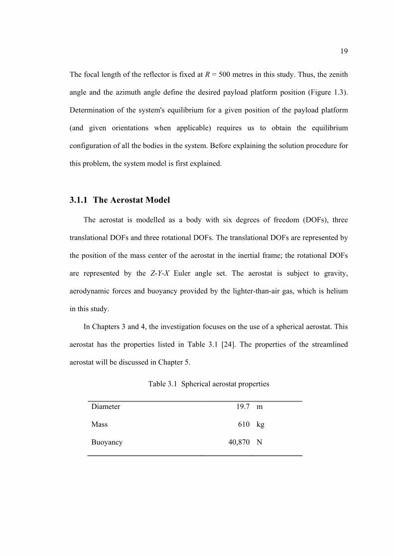
In Chapters 3 and 4, the investigation focuses on the use of a spherical aerostat. This
aerostat has the properties listed in Table 3.1 [24]. The properties of the streamlined
aerostat will be discussed in Chapter 5.
Table 3.1 Spherical aerostat properties
Diameter 19.7 m
Mass 610 kg
Buoyancy 40,870 N

20
3.1.2 The Payload Platform Model
The payload platform is subject to gravity, aerodynamic drag and tensions in the
tethers attached to it. It is treated differently in different simulation cases. In the triple-
tethered system or the six-tethered redundantly actuated system which will be discussed
later, it is modelled as a point mass with three translational DOFs, specified by the X, Y, Z
position of the platform in the inertial frame. In the six-tethered determinate system, it is
modelled as a 6-DOF body with both translational and rotational DOFs. The three
rotational DOFs are defined by the three Z-Y-Z Euler angle set: α, β, γ. The aerodynamic
forces are calculated by modelling the payload platform as a sphere of 6 m diameter, with
a mass of 500 kg and a drag coefficient of 0.15.
3.1.3 The Cable Model
When modelling the cables, it is assumed that the effects of bending and torsion are
small and need not be included in the model. The cable model consists of straight-line but
elastic segments joined by frictionless revolute joints, as shown in Figure 3.1. The
unstretched lengths of the main tethers are to be solved for in the statics while the leash
has a prescribed unstretched length of 100 m. Each main cable is modelled to have 10
segments and the leash is modelled to have 2 segments. These segments are treated as the
combination of a spring and a damper, with the mass lumped at the center. Forces applied
to each segment, including tension, weight, aerodynamic drag are considered in the
equilibrium calculation.

21
Figure 3.1 Cable segment model (statics)
The cable properties in this study for the triple-tethered system are listed as in Table
3.2 [24]. The cable properties for the six-tethered system will be discussed later in
Chapter 4.
Table 3.2 Cable properties
Diameter 0.0185 m
Young’s modulus 16.67×10⁹ N/m2
Leash length 100 m
Density 840 kg/m3
Normal drag coefficient 1.2
In the statics problem, every mass of the cable, the payload platform and the aerostat
must be in equilibrium. This equilibrium requires that the vector resultant of all forces
Segment i+1
mass lumped at the center of the segments
Segment i
spring and damper
Joint i
Joint i-1

22
acting on each body is zero ( 0F =Σ ). In addition, for any bodies with rotational DOFs,
such as the payload platform in a six-tethered system and the aerostat, the vector resultant
of all moments must also be zero ( 0M =Σ ). The force equilibrium equations, and the
moment equilibrium equations when applicable, constitute the statics problem for the
system.
Fitzsimmons, et al. [23] presented a steady-state analysis of the LAR system using
this model. Part of the code developed in that work has been adopted and modified for
the purposes of this work. In the following section, Fitzsimmons’ statics solution is
discussed, as it relates to the triple-tethered aerostat system with a spherical aerostat.
Later, in Chapters 4 and 5, the extension of this solution to other cases will be discussed.
3.2 Fitzsimmons’ Statics Solution
The first attempt to solve the statics problem for this system was based on simply
writing the force/moment balance equations for all masses in the system, and then using a
nonlinear equation solver to find the mass positions. This proved to yield an ill-
conditioned Jacobian matrix and could only be solved for very elastic tethers. After some
fruitless effort in this direction, this approach was abandoned and instead Fitzsimmons’
statics solution was used.
Fitzsimmons [23] solved the statics problem for a triple-tethered system
configuration by finding the tether profiles under a prescribed steady wind condition. In
the configuration considered, all tethers, including the leash, meet at the confluence point
(CP) --- the center of mass of the payload platform. The information to be determined
includes the unstretched tether lengths, positions of all objects in the system. To do this

23
requires that we first specify the necessary system information, which are the desired CP
position, tether winch positions, tether properties, numbers of nodes in each tether,
aerostat characteristics etc.
Fitzsimmons’ approach obtains the tether profiles one by one. For each tether, a no-
wind analysis is used to provide an initial guess of unstretched lengths and winch forces.
The winch force is then adjusted to achieve position coincidence of the tether top node
and the CP. Once this is accomplished for all tethers, the resultant force at the CP is
checked. If it is not zero, the unbalanced resultant force is used to adjust the unstretched
lengths of tethers, and the tether profile calculations are repeated. This process continues
until the algorithm has converged (i.e., the resultant force at the CP is close enough to
zero).
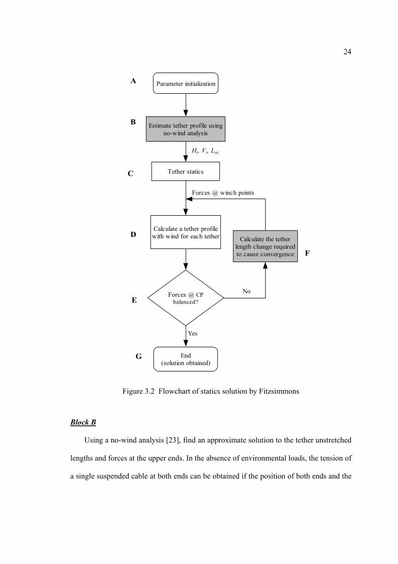
Figure 3.2 illustrates this procedure. The shadowed blocks in the diagram are the
main parts that will later require modifications in order to adapt Fitzsimmons’ approach
to the six-tethered aerostat system. The steps (blocks in Figure 3.2) are explained in more
detail as follows:
Block A
Initialize parameters. These parameters include: the number of tethers; tether
properties; the length of the leash; locations of the base of each tether from the origin
(center of reflector); payload properties; the specified CP position defined by a zenith
angle, an azimuth angle, and a focal length R; the steady wind condition; and the aerostat
characteristics.
24
Parameter initialization
Estimate tether profile usingno-wind analysis
Tether statics
Calculate a tether profilewith wind for each tether
Forces @ CPbalanced?
Calculate the tetherlength change requiredto cause convergence
End(solution obtained)
Hi, Vi, Loi
Forces @ winch points
No
Yes
A
B
C
D
E
F
G
Figure 3.2 Flowchart of statics solution by Fitzsimmons
Block B
Using a no-wind analysis [23], find an approximate solution to the tether unstretched
lengths and forces at the upper ends. In the absence of environmental loads, the tension of
a single suspended cable at both ends can be obtained if the position of both ends and the

25
unstretched length of the cable are prescribed [26].
Figure 3.3 shows the i-th elastic cable suspended in a vertical plane, which is the
configuration we are interested in. Assuming that the unstretched length of the cable is L0i,
the cross-sectional area of the unstretched cable is Α0, the Young’s modulus of the cable
is Ε, and the cable end positions are (0, 0) and (li, hi) in a reference frame as shown in
Figure 3.3, the solutions for the horizontal and the vertical components of the tension at
the top end, Hi and Vi respectively, can be obtained from the following two nonlinear
algebraic equations [26]:
Figure 3.3 The strained cable profile
⎪⎭
⎪⎬⎫
⎪⎩
⎪⎨⎧
⎥⎥⎦
⎤
⎢⎢⎣
⎡⎟⎟⎠
⎞⎜⎜⎝
⎛ −+−
⎥⎥⎦
⎤
⎢⎢⎣
⎡⎟⎟⎠
⎞⎜⎜⎝
⎛++⎟⎟
⎠
⎞⎜⎜⎝
⎛−=
=⎥⎦
⎤⎢⎣
⎡⎟⎟⎠
⎞⎜⎜⎝
⎛ −−+= −−
2/122/12
0
0
0
110
0
0
1121
3 2, 1,,sinhsinh
i
ii
i
i
i
ii
i
iiii
i
ii
i
i
i
iiiii
HWV
HV
WLH
WV
EALW
h
iH
WVHV
WLH
EALH
l
(3.1)
where Wi is the weight of the tether which is a function of L0i.
Vi
Ηi
Ti Wi
(li, hi)
(0, 0) X
Z
O

26
The equilibrium requires that the resultant of all forces acting at the CP is zero. This
leads to three equilibrium force equations at the CP
0=Σ xF , 0=Σ yF , 0=Σ zF
We can expand these as components in the inertial frame OIXIYIZI as follows:
0
0
0
3
1
3
1
3
1
=++
=
=
∑
∑
∑
=
=
=
lzpi
i
iyi
ixi
TWV
H
H
(3.2)
where Hxi, Hyi, are the components of Hi along XI- and YI-directions; Wp is the payload
weight; and Tlz is the ZI-component of the leash tension which is purely vertical in the no-
wind case. It should be noted that Tlz can be easily obtained as the weight and lift of the
aerostat and weight of the leash are known. Assembling the three force equilibrium
Equations (3.2) and the tether static equilibrium Equations (3.1) together --- nine
equations in total, we can solve for the nine unknowns, Hi, Vi and L0i (i = 1, 2, 3) of the
tethers, using a Newton-Raphson nonlinear equation solver [27].
The Newton-Raphson solver must be given an initial guess for the unknowns
before it begins iterating. The initial guess for the variables Hi and Vi (i = 1, 2, 3) was
found by first solving for an approximation to the tether tensions Ti (i = 1, 2, 3) using
⎥⎥⎥
⎦
⎤
⎢⎢⎢
⎣
⎡
−−=
⎥⎥⎥
⎦
⎤
⎢⎢⎢
⎣
⎡
⎥⎥⎥⎥⎥⎥⎥
⎦
⎤
⎢⎢⎢⎢⎢⎢⎢
⎣
⎡
plzzzz
yyy
xxx
WTTTT
dd
dd
dd
dd
dd
dd
dd
dd
dd
00
3
2
1
3
3
2
2
1
1
3
3
2
2
1
1
3
3
2
2
1
1
(3.3)

27
Figure 3.4 Tethers in a 3-D space
where (dxi, dyi, dzi) is the ground end position of tether i, i = 1, 2, 3, in the inertial frame
with its origin at the center of payload (Figure 3.4) and 222ziyixii dddd ++= . Then,
using those values of Ti, the horizontal and vertical components were found from
⎥⎥⎥
⎦
⎤
⎢⎢⎢
⎣
⎡
⎥⎥⎥⎥⎥⎥⎥
⎦
⎤
⎢⎢⎢⎢⎢⎢⎢
⎣
⎡
=⎥⎥⎥
⎦
⎤
⎢⎢⎢
⎣
⎡
3
2
1
3
3
2
2
1
1
3
3
2
2
1
1
3
3
2
2
1
1
321
321
321
TTT
dd
dd
dd
dd
dd
dd
dd
dd
dd
VVVHHHHHH
zzz
yyy
xxx
yyy
xxx
(3.4)
The initial guess for the unstretched lengths L0i (i = 1, 2, 3) are assumed to be
ii dL 99.00 = i = 1, 2, 3 (3.5)
Block C
We can now find the winch force, Ti, for each tether. This is done by considering the
winch #1 (dx1, dy1, dz1)
CP X
Y Z
d1
winch #3 (dx3, dy3, dz3)
winch #2 (dx2, dy2, dz2)
dz3
dx3 dy3
d3

28
equilibrium of external forces acting on each tether (see Figure 3.3):
0WVHT =+++ iiii (3.6)
where Ti, Hi, Vi and Wi are the vector form of the scalar forces Ti, Hi, Vi and Wi
respectively. The forces Hi and Vi, acting at the top node are known from Block B, while
the weight of the tether Wi is known from the tether properties and unstretched length L0i
calculated from Block B.
Block D
Using the unstretched length from the no-wind analysis of Block B and the winch
force from Block C, we can now calculate the profile of each tether in the presence of the
prescribed wind. Each tether profile, including the profile of the leash is solved
independently, segment by segment starting from the far-from-CP end and ending at the
CP end (all tethers meet at the CP). The tether profile calculation is illustrated in the
flowchart shown in Figure 3.6.
The steps shown in Figure 3.6 are explained as follows:
D1. For each segment, we use the known tension at the segment end far from the CP to
calculate the tension at the segment end close to the CP, as well as the orientation
of the segment.
Figure 3.5 shows the forces acting on the first segment of a tether attached
to the ground. Since the unstretched length of the tether is fixed, the unstretched
length of each segment is known; the weight W1 is known; D1, the aerodynamic
drag of the first segment, is a function of the tether position and orientation, when
the wind is known. Angles β1, Γ1 as shown in Figure 3.5 define the orientation of

29
the tether segment (a third angle is not necessary as we ignore the torsion in the
segment). Thus, when Twinch (with components Tx0, Ty0, Tz0) is known, T1 (with
components Tx1, Ty1, Tz1), and β1, Γ1 can be derived from the equilibrium condition.
Summing up all the forces applied to the segment and moments about the center of
mass (CM in Figure 3.5) of the segment in the inertial frame, we have
Figure 3.5 Tether segment analysis
0coscossincoscoscossincos0sincoscossincoscos
0
00
11111010
111010
110
110
110
=+−−=+−−
=++
=++=++
ββββββ
1y1x1y1x
1x1z1x1z
zz
yyy
xxx
ΓTΓTΓTΓTΓTΓTΓTΓT
WTT
DTTDTT
(3.7)
where the distance from the winch to the center of mass and that from node 1 to
the center of mass are equal and cancel out in the moment equations. The drag
forces Dx1 and Dy1 are nonlinear functions of β1 and Γ1. The 5 unknowns: Tx1, Ty1,
Tz1, β1, Γ1 can then be solved from the 5 nonlinear equations in Equations (3.7)
using the Newton-Raphson nonlinear equation solver [27].
node 1D1 CM
Twinch (Tx0, Ty0, Tz0)
Y
T1 (Tx1, Ty1, Tz1)
β1Γ1
X
Z
W1
Vwind

30
Single-segmentcalculation (Figure 3.5)
Lastsegmentreached?
No
Top nodecoincideswith CP?
Modify winch tensionaccording to the
position error of thetop node of the tether
Tension @ the far-from-CPend of the segment
Tension @ the close-to-CPend and orientation ofthe segment
Yes
Yes
Yes
Is the tethera maintether?
No
It is the leash
No
Set the base(aerostat) position
Winch forces,Aerostat lift and drag
D1
D2
D3
D4
D5
D6
Block D
Figure 3.6 Tether profile calculation (Block D in Figure 3.2) D2. Starting from the end which is the farthest from the CP, the single-segment
calculation of Block D1 is repeated until the segment connected to the CP is
reached. With tensions at all ends and the orientations of all segments obtained, the

31
tether profile is known, and the position of the end attached to the CP, can be
calculated from the unstretched length solved from the no-wind analysis and the
Young’s modulus of the tether.
D3. Check whether the tether is a main tether or the leash --- the leash is a special case
as its unstretched length is known a priori.
D4. If the tether is a main tether, check whether the position of its top end, denoted as
(xi, yi, zi) for the i-th tether, coincides with that of the CP (xCP, yCP, zCP) within a
certain tolerance:
pCPiCPiCPi zzyyxx ε≤−+−+− 222 )()()( (3.8)
where εp is set to 0.001 m, which is about one millionth of the distance from the
winch to the CP.
Because the no-wind solution of the tension at the base end was used, the
position of the top end of the tether will probably not coincide with the position of
the CP at the first iteration.
D5. Adjust the winch tension according to the position error. The adjustment made at
the winch relies on an approximation of the relation between the tether tension and
the change of tether length after being stretched. This approximation is based on
the assumption that the tether is straight.
Under this assumption, tether i with an unstretched length of L0i and a
straight-line distance between the two ends of di will have a tension of
⎟⎟⎠
⎞⎜⎜⎝
⎛−=
−= 1
00
0
00
i
i
i
iii L
dEA
LLd
EAT (3.9)

32
Figure 3.7 illustrates the rationale of the algorithm. The top end of the
tether in this step is shown as point P. The tension in the tether can be expressed in
vector form as
Figure 3.7 Approximation used in tether analysis
||||
1|||||||| 0
0i
i
i
i
i
iii L
EATPPP
PPT ⎟⎟
⎠
⎞⎜⎜⎝
⎛−−=−= (3.10)
where Pi is the position vector from winch location i to P. When point P does not
coincide with its desired position --- the CP, an adjustment is made to the winch
tension. This adjustment is intended to move the top end to point Q, which is
between point P and the CP. If the position vector from the winch i to the CP is P0i,
then the position vector from the winch location i to Q, can be expressed as
Qi = Pi + α (P0i – Pi) = α P0i + (1 – α) Pi (3.11)
where α is a number between 0 and 1. Therefore, we know the resulting change in
the tension when we move the top node from P to Q:
winch i
P
CP
Q
di

33
⎭⎬⎫
⎩⎨⎧
⎟⎟⎠
⎞⎜⎜⎝
⎛−−⎟⎟
⎠
⎞⎜⎜⎝
⎛−=∆
||||1
||||||||
1||||
000
i
i
i
i
i
i
i
ii LL
EAQQQ
PPP
T (3.12)
In Fitzsimmons’ statics solution, α in Equation (3.8) is set to 0.75 initially. If the
convergence proceeds smoothly, this will allow point P to reach the CP after a
number of iterations. Some rules are used to increase or decrease α during the
iterations if the convergence is not smooth. These rules improve convergence and
robustness of the algorithm.
Figure 3.8 Leash analysis
D6. For the leash, the solution is not iterative. Figure 3.8 illustrates the leash analysis.
The leash is modelled as two segments. The aerostat’s lift, La, and drag, Da, can be
obtained from the prescribed wind condition and the aerostat properties. Similar to
the tethers attached to the ground, we start the calculation at the segment farthest
from the CP. Once the tether segment calculation is completed, the tensions at the
CP
Aerostat
La
Da

34
CP end and the leash profile are obtained. The aerostat position in the inertial
frame can be obtained from the CP position and the relative position of the aerostat
end from the CP.
Block E
At the output of Block D, the top end of all three tethers and the lower end of the
leash now all meet at the CP. The tension that each cable exerts on the CP is also known.
In equilibrium, the resultant force at the CP should be zero within a certain tolerance:
fzyx FFF ε≤Σ+Σ+Σ 222 )()()( (3.13)
where εf is set to 1.5 N, and relaxed to 5.0 N when the number of iterations has exceeded
50.
Since each tether has been analyzed independently, using a value of the unstretched
length determined from the no-wind analysis, the resultant force will, in general, not be
zero at the first iteration.
Block F
The resultant force at the CP is used to generate a length adjustment for each tether.
The algorithm used relies on an approximation of the relation between the change in
tension due to a change in the unstretched length of a tether, based on the assumption that
the tether is straight --- without considering the effects of weight and wind.
If a tether in Figure 3.4 has an unstretched length of L0i, and a straight-line distance
between its two ends of di, then a change in the unstretched length of ∆L0i, will lead to a
change in the tension in the tether ∆Ti of

35
)()(
000
00
0
0
00
000
iii
ii
i
ii
ii
iiii LLL
LdEA
LLd
LLLLd
EAT∆+
∆−=⎟⎟
⎠
⎞⎜⎜⎝
⎛ −−
∆+∆+−
=∆ (3.14)
In this analysis, a reference frame with its origin at the CP (Figure 3.4) is employed.
For each tether, the winch point is located at (dxi, dyi, dzi). When the unstretched length
has a change of ∆L0i, the force changes in the X-, Y- and Z-directions as in Figure 3.4,
∆Txi, ∆Tyi, ∆Tzi, are
)(
)(
)(
000
00
000
00
000
00
iii
izizi
iii
iyiyi
iii
ixixi
LLLLdEAT
LLLLd
EAT
LLLLdEAT
∆+∆
−=∆
∆+∆
−=∆
∆+∆
−=∆
(3.15)
Therefore, when the resultant force at the CP is not zero, we assume that we can
adjust the unstretched length of tether i by an amount ∆L0i, so that the resultant force
change corresponding to the length changes will cancel out the unbalanced force at the
CP. The desired unstretched length changes are found from the following equations:
∑∑
∑∑
∑∑
==
==
==
=∆+
∆−++
=∆+
∆−++
=∆+
∆−++
3
1 000
00
3
1
3
1 000
00
3
1
3
1 000
00
3
1
0)(
0)(
0)(
i iii
izilzp
ii
i iii
iyilypy
iyi
i iii
ixilx
ipxxi
LLLLd
EATWV
LLLLd
EATDH
LLLLd
EATDH
(3.16)
where Hxi, Hyi, Vi are the XI-, YI- and ZI-components of the tension of tether i, Dpx and Dpy
are the XI- and YI-components of the aerodynamic drag on the payload, and Tlx, Tly and Tlz
are the XI-, YI- and ZI-components of the leash tension. This is a system of 3 nonlinear
equations in 3 unknowns ∆L01, ∆L02 and ∆L03.

36
This problem is solved by the same Newton-Raphson algorithm as was used in
Block B [27]. The program returns to Block D with the new unstretched lengths of the
tethers Loi+ ∆L0i.
Block G
Once the resultant force at the CP satisfies Inequality (3.13), we have a solution for
the equilibrium. The obtained tether profile information can then be used to provide an
initial condition for the dynamics simulation.
3.3 Implementation and Modifications of Fitzsimmons’ Solution
Fitzsimmons’ statics solution was incorporated into our simulation for the case of a
triple-tethered system. In doing so, Block A (parameter initialization) in Figure 3.2 was
modified to accept parameters already defined in our main program and the result of
Block G was modified to provide initial condition for the dynamics simulation which will
be discussed in Chapter 4.
Some other modifications to Fitzsimmons’ model were needed to incorporate his
solution into our work, and these are now discussed.
Wind Model
The wind model in Fitzsimmons’ work was modified to match the one used in the
dynamics model [24]. In Fitzsimmons’ wind model, illustrated on the left of Figure 3.9,
the wind speed is constant with height. By contrast, the wind model in the dynamics,
illustrated on the right of Figure 3.9, uses a power law profile [24] defined by

37
19.0
⎟⎟⎠
⎞⎜⎜⎝
⎛=
gg z
hUU (3.17)
The constant profile used in Fitzsimmons’ work was therefore replaced by the
power-law profile which is a more reasonable representation of the wind conditions over
rural terrain. Unless otherwise mentioned, this power-law wind profile is used throughout
this study and sometimes only the full wind speed Ug is mentioned.
Figure 3.9 Wind models
Jacobian Matrix Calculations
In Blocks B, D (D1 in Figure 3.6) and F of the solution procedure (Figure 3.2), a
Newton-Raphson method [27] is used to solve a system of nonlinear algebraic equations.
This requires a calculation of the Jacobian matrix of the system of equations.
Boundary layer thickness zg = 500m
Wind speed Ug Wind speed Ug Height h
Fitzsimmons’ wind model Our wind model

38
In Fitzsimmons’ implementation, this Jacobian matrix was approximated using a
finite difference scheme. To improve the robustness and speed of the solution, the finite
difference approximations of the Jacobian matrices were replaced by exact analytical
calculations in our implementation of the Newton-Raphson algorithm.
Further changes to Fitzsimmons’ statics solution will be discussed in Chapter 4 and
5 as they are related to configurations other than the three-tether spherical aerostat
configuration --- specifically, the six-tether spherical aerostat or the three-tether
streamlined aerostat configurations.
3.4 Verification of the Statics Model
Model verification is of great importance for simulation studies, as conclusions
based on an inaccurate model will be flawed. Fitzsimmons verified his work by
comparing results from different methods of analysis [23]. When incorporating his work
into ours, we had to ensure that we did not introduce errors. Our verification was done in
a few ways.
The first verification was done to compare the statics results after incorporation into
our software to those from Fitzsimmons’ original version for the same set of conditions.
This verification work was done without introducing the modifications discussed in
Section 3.3. The comparison between the statics results, showed the two sets of results to
be identical to 8 significant figures. This gives us confidence that errors were not
introduced when incorporating Fitzsimmons’ work into ours.
Our next validation consisted of running the open-loop dynamic simulations [24] (to
be discussed in Chapter 4) with the initial conditions generated by the statics analysis,

39
including the modifications of Section 3.3. This allowed us to see whether the statics
analysis generates a true equilibrium condition for the specified set of parameters. If it
does, the dynamics simulations should show the system staying at that equilibrium,
within acceptable errors; otherwise, the system will deviate from the statics solution,
presumably toward the true equilibrium. The conditions of configurations tested are listed
in Table 3.3. The wind condition used in all cases is identical. The power-law wind
profile defined by Equation (3.17) is used. The mean wind speed is 10 m/s, and the wind
angle of 180° is defined as the angle from the positive X-axis to the wind vector in the
horizontal XY-plane. The initial conditions for the dynamics simulation are the results
obtained from the statics solver.
Table 3.3 Conditions of simulation cases
Case No. Zenith angle (°) Azimuth angle (°) Wind condition
1 0 0
2 60 0
3 60 60
Power-law wind profile with a
mean wind speed of 10 m/s
and a wind angle of 180°
Figure 3.10 shows the resulting errors, plotted as errors of the CP position in and
out of the focal plane --- the plane tangent to the hemisphere (shown as the ∆za-∆az plane
in Figure 1.3). From the results, we can see that:
1) In the focal plane, the worst case is Case 2 with about 1.5 mm error; the error
out of the focal plane is worst for Case 3 at about 3 mm. It should be noted
that the scale of the multi-tethered aerostat system is on the order of 1 km, and

40
the expected positioning accuracy is to be about 1 m, therefore these errors are
very small.
2) The position errors are slightly higher for the asymmetrical Cases 2 and 3
than for the symmetric Case 1, and the error oscillations are worse for Cases 2
and 3 as well. This is likely due to the higher stiffness of the system in Case 1.
0 10 20 30 40 50 60 70 800
0.5
1
1.5
2
2.5x 10⁻³
Erro
r in
foca
l pla
ne (m
)
Payload position error
0 10 20 30 40 50 60 70 80-4
-3
-2
-1
0
1
2x 10⁻³
Time (s)
Erro
r out
of f
ocal
pla
ne (m
)
case 1case 2case 3
Figure 3.10 Errors of the CP when using statics solution as the initial states
The dynamics and statics models demonstrate a very good match. The slight
differences can be explained by the remaining model differences between the two models.
For example, in the dynamics model, the mass of each segment is split into two halves
and lumped at the segment ends. By contrast, the statics model lumps the segment’s mass

41
at the midpoint of the segment. The close match between the results of the dynamics and
statics models, each of which was developed by different people, gives us confidence that
both models are good representations of the system.

42
Chapter 4 Six-Tethered System
The computer model of a triple-tethered system developed by Nahon [24] showed
that the payload platform position could be controlled accurately by three tethers in the
presence of disturbances. However, there are some advantages to using more than three
tethers. For example, six tethers might allow us to also control the orientation of the
airborne platform. Alternatively, six tethers could be used for redundant control of the
position of the platform. These are the issues studied in this chapter.
4.1 Dynamics of the Triple-Tethered System
In Section 3.1, a statics model of the triple-tethered aerostat system with a spherical
aerostat was described. In Nahon's work [24], a similar physical model of the triple-
tethered spherical aerostat system was used to obtain the system’s dynamic equations of
motion and solve for the time histories of the system’s motion. The only difference
between the two models is in the way in which the mass of each cable segment is lumped.
Figure 4.1 shows how this is done in the dynamics simulation of [24]. The key difference
from the approach shown in Figure 3.1 is that the mass of each element is split in half and

43
each half is lumped at the end points of the element. Motion equations are formulated for
the nodes where the mass is lumped.
Figure 4.1 Cable segment model (dynamics)
A wind model is also incorporated in [24] to determine the effect of the turbulent
wind on the tethered aerostat system. This wind model consists of a mean wind profile
(as shown in right half of Figure 3.9) with turbulent gusts superimposed.
All bodies in the system model, including the cable nodes, the payload platform,
and the aerostat, are modelled as bodies with only translational DOFs. The motion
equations governing the motion of the system are set up by applying Newton’s second
law of motion ( aF m=Σ ) to each body to relate its acceleration vector and the vector
resultant of all forces applied to it [24].
In Nahon’s work [24], the spherical aerostat is modelled as a point mass with three
translational DOFs (Figure 4.2). Forces applied to the aerostat include weight Wa,
Node i (lumped mass)
Segment i
spring and damper
Node i-1 (lumped mass)

44
buoyancy Ba, aerodynamics drag Da and the leash tension Tl and damping force Pl which
are the internal forces of the top most segment of the leash. Considering added mass, its
motion equation can be expressed as:
aaaallaaa mm aPTDWB )( +=++++ (4.1)
where ma and maa are the mass and added mass of the aerostat.
Figure 4.2 The tethered aerostat system model in 2-D [24]
The payload is also modelled as a point mass. Forces applied to it include its
weight Wp, aerodynamic drag Dp and cable forces from the segments attached to it which
Aerostat
Payload
Leash
YI
XI
ZI
OI
Tether
node 1
node 2 segment 1
segment n
node 3
node n-1
node n+1
segment n-1
segment 2
node n
45
are the tensions Ti and damping forces Pi, where i = 1, …, 4, from all 4 cables, including
the leash. The motion equation can be summed up as
pappi
iipp mm aPTDW )()(4
1
+=+++ ∑=
(4.2)
where mp and map are the mass and added mass of the payload.
Forces applied to each node of each tether include gravity, aerodynamic drag and
internal tensions and damping forces. Damping force is created by the friction between
braids of the cable [24]. It is assumed to be linear with the strain rate and calculated using
[24]
)( 1zi
ziv
zii C −−== vvPP (4.3)
where Cv is the damping coefficient, 10,000 N⋅s/m for this application, and ziv is the
velocity of the i-th node in the tangential Zti-direction (Figure 2.1).
Summing up all the forces in the inertial frame, the motion equation for node i can
be written as
iaiiiiiiiiii mm aDWDWPTPT )()(21)( 1111 +=+++++−+ −−−− (4.4)
where Wi, Di, Ti and Pi are the weight, drag, tension and damping force in the i-th
segment respectively, mi and mai are the lumped mass and its added mass at node i, while
ai is the acceleration of the node.
The above Equations (4.1), (4.2) and (4.4) contain 90 motion equations set up at 30
node points: each main tether is discretized into 10 segments and the leash is modelled
using 2 segments. Thus each of the main tethers has 11 nodes and the leash has 3 nodes.
The motion equations are set up at each node except the base node of the main tethers.
The top nodes of the tethers and the bottom node of the leash are the same point as the

46
payload node. The top node of the leash is also the aerostat node. These 90 motion
equations are second-order ordinary differential equations (ODEs). In order to use a
conventional numerical integrator, each of the motion equations is rewritten as two first
order differential equations, thus resulting in 180 first-order ODEs.
Moreover, PID controllers are implemented to control the winches, which are
assumed to be located at the base of tethers. The winches adjust the unstretched length of
each tether and thus control the position the payload platform. In particular, the winch
controllers operate on the position errors of the CP [24]. A 2-D illustration of the control
scheme is shown in Figure 4.3. Assuming the desired location of the CP is at pd (xd, yd,
zd), its actual location is at p (x, y, z), and the i-th winch (i = 1, 2, 3) is at wi (xwi, yw
i, zwi),
we can define the desired and actual distances from each winch to the CP as [24]
Ldi = || pd - wi ||, Li = || p - wi || (4.5)
Figure 4.3 Controller 2-D illustration [24]
Desired location
P
Pd
Actual location
Wi Wj
Ldi
Li

47
And the winch controller operates according to [24]
∫ −−−−−−= dtLLkLLkLLkll iidi
iidp
iidd
iu
iu )()()(101
&& (4.6)
where iul 1 is the unstretched length of the first (lowermost) segment of tether i, while i
ul 10
is its initial unstretched length, and kd, kp and ki are the PID controller gains. In order to
integrate the error, 3 more first order differential equations are added to the system.
These 183 first order differential equations are solved using a fourth order Runge-
Kutta integrator [27], which gives accurate solutions to a wide range of scientific
problems.
Some main findings of the dynamics simulation are [24]:
1) The system is less well behaved at large zenith angles of the payload platform
while it is not very sensitive to changes of the azimuth angle;
2) The system acts as a low-pass filter to turbulent gusts; and
3) The motion response of the payload platform may be controlled within
centimeters of its desired position in the presence of turbulent gusts.
In this chapter, we are interested in extending the prior work on a triple-tethered system
[24] to a six-tethered system.
4.2 Redundantly Actuated System
In the LAR multi-tethered system, the tethers, the payload platform and the
ground form a closed-link mechanism. If we are only interested in controlling the
position of the payload platform, the system is redundantly actuated if there are more
than three adjustable tethers.

48
4.2.1 Actuation Redundancy
Redundancy is a feature of systems in a variety of fields, such as aerospace
engineering, electrical engineering, and mechanical engineering. Redundancy can be
primarily used to improve the reliability of a system. In many applications, redundancy
also improves the system performance. In mechanical systems, there exist two kinds of
redundancy: kinematic redundancy and actuation redundancy [28].
Kinematic redundancy implies a mechanism has more degrees of freedom (DOFs)
than the number of DOFs needed to accomplish the task. Generally speaking, kinematic
redundancy improves manipulability, is used to avoid obstacles, structural limitations or
to optimize various performance criteria [28], [29].
Actuation redundancy implies that the system has more actuators than DOFs. It is
found only in closed-loop mechanisms, and has an important effect on the determination
of the forces and moments. The difference between the number of actuators and the
number of DOFs is the degree of actuation redundancy.
In the LAR multi-tethered system, when six tethers are used to control the
position of the playload platform, we say the system has three degrees of actuation
redundancy. The actuation redundancy brings some advantages to the system:
1) The reliability of the system is increased. That is, even if one of the tethers
fails, the system stays controllable and can continue to operate;
2) The tension in each of the tethers can be decreased and the loading made more
uniform among the tethers, even in the presence of asymmetric wind
conditions.
3) The size of tethers can be smaller since the tensions in the tethers are smaller.
49
4) The accuracy of positioning the receiver may be improved, such that the
system becomes more stable in the presence of wind turbulence.
However, concurrently, some disadvantages are introduced:
1) The total tether weight is increased;
2) The number of winches is increased;
3) The total cost to build the system is increased;
4) The system becomes more complicated. The amount of necessary
computation increases. In particular, substantial complexity is also added in
finding the static equilibrium configuration and, possibly, in controlling the
system because the forces in the system cannot be determined uniquely.
4.2.2 Redundancy in Statics
The system has three degrees of actuation redundancy, i.e., there are three more
tethers than the minimum number necessary to maintain its equilibrium. When
considering the force balance at the confluence point, the number of force equilibrium
equations is three, but we have to find the tensions in six tethers. Thus the tension in each
tether can not be determined uniquely, and the problem is considered to be statically
indeterminate. The redundancy gives us the opportunity to utilize optimization techniques
to solve the problem.
Fitzsimmons had an alternative solution for six-tether configuration. However,
that solution was not general and could not handle arbitrary zenith and azimuth angles of
the six-tethered system. It is more desirable to consider a more general solution. Looking
back at Fitzsimmons’ statics solution for the three-tether configuration of the system

50
(Section 3.2), we find that only two of the main steps need to be modified to extend the
solution to a six-tether configuration. These are the shadowed blocks, B and F, in Figure
3.2. In both of these blocks, for the six-tether case, we will have more unknowns than
equations, and we therefore have a choice of solutions.
Optimization techniques are used to find the best tension distribution among all
the solutions to achieve the desired performance. The statically indeterminate problem
then becomes a constrained optimization problem. The formulation and solution of the
problem are now discussed in more detail.
4.2.3 Constrained Optimization Problem
In a general mathematical form, a constrained optimization problem is to
determine an unknown vector x* that solves the problem
minimize f(x)
subject to:
ai(x) = 0 i = 1, 2, …, p
bj(x) ≤ 0 j = 1, 2, …, q
where f(x) is called the objective function, it is a scalar quantity which can assume
different forms; the equations ai(x) = 0 are the equality constraints, while bj(x) ≤ 0 are the
inequality constraints.
4.2.4 Nonlinear Optimizer CFSQP
The software CFSQP (C code for Feasible Sequential Quadratic Programming)
[30] is a set of C functions for the optimization of a set of smooth objective functions

51
subject to general smooth constraints. It was originally developed at the Institute for
Systems Research, University of Maryland. We obtained the non-profit version in late
1999 at no cost. Since then, the software has been further developed and transferred to
AEM Design, Atlanta [31].
In the case as our problem, CFSQP tackles optimization problems of the form
minimize max{fi(x)} i = 1, 2, …, p
where x must satisfy the lower and upper bounds
bl ≤ x ≤ bu
and constraints:
Nonlinear inequalities: gj(x) ≤ 0 j = 1, 2, …, ni
Linear inequalities: gj (x) ≤ 0 j = ni+1, …, ti
Nonlinear equalities: hj (x) = 0 j = ti +1, …, ne
Linear equalities: hj (x) = 0 j = ne +1, …, te
All the functions, including fi(x), gj(x), hj(x) must be smooth.
Use of this solver does not require a feasible initial guess, i.e., a value of x, which
satisfies all constraints. If the initial guess provided by the user is infeasible, CFSQP first
generates a feasible point for these constraints; subsequently the successive iterates
generated by CFSQP all satisfy these constraints. The user must provide software
functions that define the objective functions and constraint functions. Further, the user
may either provide software functions to compute the respective gradients of fi(x), gj(x)
and hj(x) or require that CFSQP estimate them by forward finite differences [30].

52
4.2.5 Implementation in the Statics
When using Fitzsimmons’ approach to obtain the statics solution, it is difficult to
implement a single global performance measure for the problem because the statics
problem has been split into sub-problems, two of which (Blocks B and F) need
modification. We must therefore choose the objective functions in these sub-problems
with caution. The approach taken to do this is now described.
Block B: No-wind Analysis
In the sub-problem of Block B in Figure 3.2, we choose to minimize the sum of
the tether tensions squared, with the intention of minimizing the internal forces. This is
chosen after comparing the results from different objective functions, as will be shown in
Section 4.2.8.
Thus, the objective function to be minimized is
∑=
++=6
1
222 )(i
iyixiB VHHf (4.7)
while the constraints are the force equilibrium equations at the CP:
0
0
0
6
1
6
1
6
1
=++
=
=
∑
∑
∑
=
=
=
ilzpi
iyi
ixi
TWV
H
H
(4.8)
where Hxi and Hyi are the components of Hi; Wp is the weight of the payload platform; Tlz
is the leash tension under the no-wind condition.

53
The Equations (3.1) relating tension components Hi, Vi and the unstretched
lengths L0i also become equality constraints, two for each tether (repeated here for
convenience):
⎪⎭
⎪⎬⎫
⎪⎩
⎪⎨⎧
⎥⎥⎦
⎤
⎢⎢⎣
⎡⎟⎟⎠
⎞⎜⎜⎝
⎛ −+−
⎥⎥⎦
⎤
⎢⎢⎣
⎡⎟⎟⎠
⎞⎜⎜⎝
⎛++⎟⎟
⎠
⎞⎜⎜⎝
⎛−=
=⎥⎦
⎤⎢⎣
⎡⎟⎟⎠
⎞⎜⎜⎝
⎛ −−+= −−
2/122/12
0
0
0
110
0
0
1121
6,...,1,sinhsinh
i
ii
i
i
i
ii
i
iiii
i
ii
i
i
i
iiiii
HWV
HV
WLH
WV
EALW
h
iH
WVHV
WLH
EALH
l
(4.9)
where Wi is the weight of the tether, li and hi are the horizontal and vertical components
of the distance between the two endpoints of a tether (see Figure 3.3). Thus, equations
(4.8) and (4.9) constitute 15 equations in 18 unknowns (Hi, Vi and L0i for i = 1, …, 6), and
the optimal solution will be found by minimizing the objective function Equation (4.7).
Furthermore, in order to avoid obtaining a solution with slack tethers, we place a
constraint on each tether, to ensure that the vertical tension Vi at the top end of the tether
is greater than the weight of the tether Wi. Therefore, we include six more constraints as
follows:
0≤− ii VW i = 1, ..., 6 (4.10)
Thus, the underdetermined problem noted previously with 18 unknowns and 15
equality constraints is augmented to include these 6 inequality constraints.
Block F: Unstretched Tether Length Adjustment
The sub-problem of Bock F in Figure 3.2, in which we must determine the
unstretched tether length changes, also becomes indeterminate. This problem consists of

54
finding six unknowns, ∆L0i for i = 1, ..., 6, while satisfying the three equality constraints
which are the force equilibrium equations at the CP:
∑∑
∑∑
∑∑
==
==
==
=∆+
∆−++
=∆+
∆−++
=∆+
∆−++
6
1 000
00
6
1
6
1 000
00
6
1
6
1 000
00
6
1
0)(
0)(
0)(
i iii
izilzp
ii
i iii
iyilypy
iyi
i iii
ixilx
ipxxi
LLLLd
EATWV
LLLLd
EATDH
LLLLd
EATDH
(4.11)
In general, for the triple-tethered system, we find that the winch forces and the
unstretched lengths of the tethers in the final statics solution are very close to those in the
no-wind analysis. This implies that the effect of the wind on the tether equilibrium is not
very significant. For this reason, in this sub-problem, we choose to minimize the sum of
the length change squared as
∑=
∆=6
1
20
iiF Lf (4.12)
in the expectation that the optimal solution thus obtained will be close to the solution of
the no-wind analysis. This makes the minimization of the tension norms in Block B
approximately global.
When implementing CFSQP in the existing program to solve this problem, we
again provide the exact analytical form for the Jacobian matrix instead of using a finite
difference method which might slow down the convergence.
It should be noted that the optimizer can also be used for cases in which there
exists a unique solution (e.g. the triple-tethered case). In the interest of consistency, we
use this optimization solver to solve the determinate statics problem of the triple-tethered
systems as well.

55
4.2.6 Dynamics of the Six-Tethered System
The tethered aerostat dynamics model in [24] was set up in such a way that it is
very easy to expand the model from a three-tether configuration to a six-tether
configuration. In Nahon’s model, forces exerted on each segment of the tethers, tension
and drag, are calculated in generic subroutines. Except for some minor changes, the
dynamics model of the tethered aerostat system stays almost untouched when simulating
the six-tethered aerostat system. It should be noted that the controller used, described in
Section 4.1, is purely kinematically based. Normally, we would expect that a
redundantly-actuated system should also include some form of force control.
4.2.7 Statics Results and Verification
We are now interested in seeing how the statics and dynamics solutions
correspond to each other, as we did in the case of 3 tethers. Some parameter changes used
for the six-tether cases are listed in Table 4.1. They include a decrease in the tether base
radius and the cable diameter. These are indicative of one advantage that the 6-tether
configuration brings to the system: with more tethers employed in the system, the system
size can be reduced [23].
Table 4.1 Parameter changes
Parameter
Configuration Base radius (m) Cable diameter (m)
3-tether configuration 1200 0.0185
6-tether configuration 635 0.0142

56
Figure 4.4 shows the dynamic simulation results for the six-tethered system with
the new statics solution as the initial condition. The same simulation cases are used as
those in Table 3.1 for easy comparison. From Figure 4.4, we can see that the largest
steady-state error in the focal plane is about 1.1 mm which occurs in Case 2; the largest
error out of the focal plane is close to 2.1 mm which occurs in Case 3.
The mismatch is of the same order as that in the three-tether configuration (Figure
3.10). This verifies the correctness of the statics and dynamics models of the six-tethered
aerostat system.
0 10 20 30 40 50 60 70 800
0.5
1
1.5x 10⁻³
Erro
r in
foca
l pla
ne (m
)
Payload position error
0 10 20 30 40 50 60 70 80-3
-2
-1
0
1
2x 10⁻³
Time (s)
Erro
r out
of f
ocal
pla
ne (m
)
case 1case 2case 3
Figure 4.4 Matching simulations for the six-tethered spherical aerostat system

57
4.2.8 Optimization Results and Discussion
A few different objective functions were evaluated in the no-wind analysis, Block
B in Figure 3.2, before deciding on the objective function described in Section 4.2.5.
Some results of the study are presented and discussed in this section. The different
objective functions evaluated are shown in Table 4.2, where Ti is the magnitude of the
tension at the top node of tether i, Ti = 22ii VH + , di is the straight line distance
between the base node (winch point) and the top node of tether i (Figure 3.4). Objective
functions 1 and 2 are chosen with the intention to minimize the internal forces; objective
functions 3 and 4 are chosen with the intension to maximize the stiffness of the system
since the shorter L0i, the higher tension in tether i, and the stiffer the system.
Table 4.2 Objective functions for no-wind analysis
No. Objective Function Note
1 ∑=
6
1iiT To minimize the sum of tensions
2 ∑=
6
1
2
iiT To minimize the sum of tensions squared
3 ∑=
6
1
20
iiL To minimize the sum of unstretched tether lengths squared
4 ∑=
⎟⎟⎠
⎞⎜⎜⎝
⎛6
1
2
0
i i
i
dL
To minimize the sum of squared ratios between the
unstretched length and the straight-line distance between
the two ends of the tether
Figure 4.5 shows the resulting tensions in the tethers with different objective

58
0
1000
2000
3000
4000
5000
6000
7000
8000
9000
1 2 3 4 5 6
Obj 1Obj 2Obj 3Obj 4
functions used in Block B (the no-wind analysis) as discussed in Section 4.2.5 and with
the consideration of the wind. Again, the cases shown are the same as described in Table
3.1.
From the statics results shown in Figure 4.5, we can see:
1) The same result is obtained for the case with zero zenith angle and azimuth
angle with all the objective functions tested.
2) The results with objective function 2 show the most evenly distributed
tensions among all tethers in all the cases tested. The most tensioned tether,
tether 1 in Case 2 or tether 2 in Case 3, has the smallest tension; the least
tensioned tether, tether 6 in Case 2 or tether 3 in Case 3, has the highest
tension. This more even distribution led us to select objective function 2 for
the no-wind analysis.
(a) Case 1: θza = θaz = 0
(N)
Tether No.
Tension

59
0
5000
10000
15000
20000
25000
30000
1 2 3 4 5 6
Obj 1Obj 2Obj 3Obj 4
(b) Case 2: θza = 60°, θaz = 0
(c) Case 3: θza = θaz = 60°
Figure 4.5 Tether tensions in statics using different objective functions
(Conditions: wind speed = 10 m/s, wind angle = 180°)
0
5000
10000
15000
20000
25000
30000
1 2 3 4 5 6
Obj 1Obj 2Obj 3Obj 4
Tether No.
Tension
(N)
Tether No.
Tension
(N)

60
The results for Case 1 led to the question whether the solution for the
configuration θza = θaz = 0° is unique. We notice that in all the objective function in Table
4.2, all tethers are treated equally. We therefore choose an asymmetric objective function
in which we only minimize the square of the tension in tether 1, i.e., f = T12. The result
using this objective function is shown in Figure 4.6, marked as “Obj 5” in the graph, and
compared to that from objective function 2. This result was then used as an initial state
for the dynamics simulation. The steady state payload position error was less than 1 mm
and can therefore be considered be a true equilibrium. Since the results for these two
objective functions are different, we conclude that the solution we previously obtained is
not unique for this system configuration.
Figure 4.6 Results for different objective functions, θza = θza = 0
0
2000
4000
6000
8000
10000
12000
14000
1 2 3 4 5 6
Obj 5Obj 2
Tether No.
Tension
(N)

61
Dynamics simulations with a wind speed of 10 m/s and wind direction of 180°
and different zenith and azimuth angles were also performed with these different
objective functions. The results are shown in Figure 4.7 and 4.8. The case numbers in
those figures are defined in Table 4.3. The objective function numbers in Table 4.3
correspond to those in Table 4.2.
Table 4.3 Case number definitions for Figure 4.7
θza = θaz = 0 θza = 60°, θaz = 0 θza = θaz = 60°
No. 1 2 3
1 11 12 13
2 21 22 23
3 31 32 33
Objective
function
4 41 42 43
Notes Case 1 in Figure 4.4 Figure 4.7 (a) Figure 4.7 (b)
From the dynamics results shown in Figure 4.7 and 4.8, we can see:
1) The maximum payload position error in the focal plane is 6.8 mm for
objective function 1, zenith angle 60° and azimuth angle 60°. The maximum
error out of the focal plane is 2.3 mm for the same objective function with the
same system configuration.
2) Objective functions 1 and 4 result in similar magnitude of errors in both
configurations, and these are worse than objective functions 2 and 3.

62
0 10 20 30 40 50 60 70 800
0.2
0.4
0.6
0.8
1
1.2
1.4x 10⁻³
Erro
r in
foca
l pla
ne (m
)
Payload position error
0 10 20 30 40 50 60 70 80-3
-2
-1
0
1
2x 10⁻³
Time (s)
Erro
r out
of f
ocal
pla
ne (m
)
case 12case 22case 32case 42
(a) θza = 60°, θaz = 0
0 10 20 30 40 50 60 70 800
0.002
0.004
0.006
0.008
0.01
Erro
r in
foca
l pla
ne (m
)
Payload position error
0 10 20 30 40 50 60 70 80-3
-2.5
-2
-1.5
-1
-0.5
0
0.5x 10
-3
Time (s)
Erro
r out
of f
ocal
pla
ne (m
)
case 13case 23case 33case 43
(b) θza = θaz = 60°
Figure 4.7 Dynamics simulation results of the payload position using different objective
functions for the statics initial condition

63
0 20 40 60 802.2
2.4
2.6
2.8
3x 10⁴
T 1 (N)
0 20 40 60 800
2000
4000
6000
8000
T 2 (N)
0 20 40 60 802000
3000
4000
5000
T 3 (N)
0 20 40 60 800
2000
4000
6000
8000
T 4 (N)
0 20 40 60 802000
3000
4000
5000
Time (s)
T 5 (N)
0 20 40 60 800
2000
4000
6000
8000
Time (s)
T 6 (N)
case 12case 22case 32case 42
(a) θza = 60°, θaz = 0
0 20 40 60 802000
4000
6000
8000
10000
T 1 (N)
0 20 40 60 802.2
2.4
2.6
2.8x 10⁴
T 2 (N)
0 20 40 60 800
2000
4000
6000
8000
T 3 (N)
0 20 40 60 801000
2000
3000
4000
5000
T 4 (N)
0 20 40 60 802000
4000
6000
8000
10000
12000
Time (s)
T 5 (N)
0 20 40 60 803500
4000
4500
5000
5500
6000
Time (s)
T 6 (N)
case 13case 23case 33case 43
(b) θza = θaz = 60°
Figure 4.8 Dynamics simulation results of the tether tensions using different objective
functions for the statics initial condition

64
3) The tension seems to stay at their initial values throughout the simulation for
all cases. The fluctuations are so small that they are not apparent in the graphs.
The errors in some cases are larger than those previously shown in Figures 3.10 and
4.4. Besides the contribution from the model differences between the statics and
dynamics model, this is largely due to the bigger error tolerance εf in Inequality (3.13)
when smaller εf can not be satisfied within 50 iterations. Nevertheless, these errors are
still quite small in comparison with the system scale. The results shown in Figure 4.7
further verify the correctness of our system model including both the statics and
dynamics components.
4.2.9 Dynamics Results and Discussion
Dynamics simulation results are further investigated for the redundantly actuated
system in order to examine its performance with and without control. As discussed in
Section 4.2.5 and 4.2.8, Objective function 2 in Table 4.2 is selected for the no-wind
analysis. A turbulence model presented in [24] was superimposed on the wind profile for
all the simulations. All simulations shown used the same wind condition: a mean wind
speed of 10 m/s and a wind angle of 180°.
Figures 4.9 and 4.10 present the simulation results with and without a controller for
zero zenith angle and zero azimuth angle (θza= θaz = 0). Figures 4.11 and 4.12 present the
simulation results with and without a controller for 60° zenith angle and 0 azimuth angle
(θza= 60°, θaz = 0). The controllers in these cases are the same as those used in Nahon’s
triple-tethered system simulation [24], which are kd = 2 s, kp = 5, ki = 5 s-1 for θza= θaz = 0

65
and kd = 4 s, kp = 1, ki = 1 s-1 for θza= 60°, θaz = 0 for easy comparison. The position errors
for the triple-tethered system are also shown along with those for the six-tethered system
in Figures 4.9 and 4.11.
Table 4.4 lists the payload position errors for the cases considered (see also Figures
4.9 and 4.11). It is interesting to see that the payload position errors are relatively small
even in the uncontrolled cases with compared to those for the triple-tethered system. For
the controlled cases, results for θza= θaz = 0 show similar magnitude of payload position
error for the 3-tether and 6-tether cases; for θza= 60°, θaz = 0, the maximum error in the
focal plane is about 0.02 m for the six-tethered system and 0.28 m for the triple-tethered
system, the maximum error out of the focal plane is 0.12 m for the six-tethered system
and 0.23 m for the triple-tethered system. The errors for the six-tethered system may be
further reduced by tuning the controller gains. These results suggest that the six-tethered
system is much stiffer than the triple-tethered system.
Table 4.4 Payload position errors for the redundantly actuated system
Conditions Maximum position error
for uncontrolled system
Maximum position error
for controlled system
Payload
position
Wind
condition
in the focal
plane (m)
out of the focal
plane (m)
in the focal
plane (m)
out of the focal
plane (m)
θza = 0
θaz = 0 0.26 0.14 0.02 0.04
θza = 60°
θaz = 0
Ug = 10 m/s
θw = 180° 0.09 0.35 0.02 0.12

66
0 10 20 30 40 50 60 70 800
0.1
0.2
0.3
0.4Payload position error
Erro
r in
foca
l pla
ne (m
)
0 10 20 30 40 50 60 70 80-0.2
-0.1
0
0.1
0.2
0.3
Erro
r out
of f
ocal
pla
ne (m
)
Time (s)
6-tether without control6-tether with control3-tether without control3-tether with control
Figure 4.9 Payload motion for θza = θaz = 0
0 20 40 60 807000
8000
9000
10000
T 1 (N)
0 20 40 60 807000
7500
8000
8500
9000
9500
T 2 (N)
0 20 40 60 805000
5500
6000
6500
7000
T 3 (N)
0 20 40 60 804000
4500
5000
5500
6000
T 4 (N)
0 20 40 60 805000
5500
6000
6500
7000
T 5 (N)
Time (s)0 20 40 60 80
7000
7500
8000
8500
9000
T 6 (N)
Time (s)
Without controlWith control
Figure 4.10 Tether tension forθza = θaz = 0

67
0 10 20 30 40 50 60 70 800
0.1
0.2
0.3
0.4
0.5
0.6
Payload position error
Erro
r in
foca
l pla
ne (m
)
0 10 20 30 40 50 60 70 80-0.6
-0.4
-0.2
0
0.2
0.4
Erro
r out
of f
ocal
pla
ne (m
)
Time (s)
6-tether without control6-tether with control3-tether without control3-tether with control
Figure 4.11 Playload motion for θza = 60°, θaz = 0
0 20 40 60 802.2
2.25
2.3
2.35
2.4x 10⁴
T 1 (N)
0 20 40 60 806500
7000
7500
8000
8500
9000
T 2 (N)
0 20 40 60 802500
3000
3500
4000
4500
T 3 (N)
0 20 40 60 801000
2000
3000
4000
T 4 (N)
0 20 40 60 802500
3000
3500
4000
4500
T 5 (N)
Time (s)0 20 40 60 80
6500
7000
7500
8000
8500
T 6 (N)
Time (s)
Without controlWith control
Figure 4.12 Tether tension for θza = 60°, θaz = 0
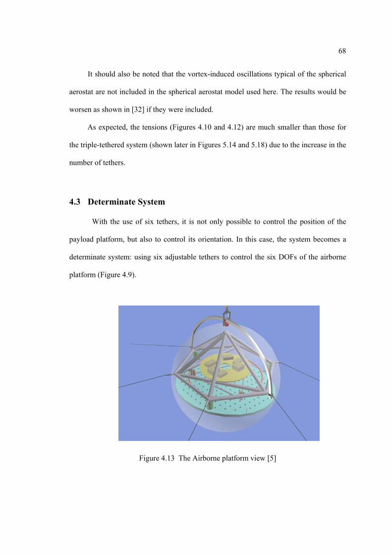
68
It should also be noted that the vortex-induced oscillations typical of the spherical
aerostat are not included in the spherical aerostat model used here. The results would be
worsen as shown in [32] if they were included.
As expected, the tensions (Figures 4.10 and 4.12) are much smaller than those for
the triple-tethered system (shown later in Figures 5.14 and 5.18) due to the increase in the
number of tethers.
4.3 Determinate System
With the use of six tethers, it is not only possible to control the position of the
payload platform, but also to control its orientation. In this case, the system becomes a
determinate system: using six adjustable tethers to control the six DOFs of the airborne
platform (Figure 4.9).
Figure 4.13 The Airborne platform view [5]

69
4.3.1 Purpose
The airborne payload platform of the telescope contains the LAR feed which
receives the radio signal from the reflector on the ground. The axis of symmetry of the
feed has to remain pointed to the center of the reflector [33], thus requiring feed
orientation control. We are therefore interested in knowing how well we can achieve the
desired orientation by adjusting the tether length alone, without using any additional
orienting mechanism. This will give us the information needed to later design a
mechanism to fine tune the feed orientation.
4.3.2 The 6-DOF Payload Platform Model
The payload platform is subject to gravity, aerodynamic forces and tensions from
the tethers attached to it as presented in Section 3.1. When modelling the platform’s 6
degrees of freedom, it is assumed that the six main tethers are attached to the payload
platform at the edge of a disk, evenly distributed, 60° apart from each other (Figure 4.9).
The leash is assumed to be attached at the mass center of the payload platform. The
orientation of the payload platform is defined by a Z-Y-Z Euler angle set (α, β, γ)
discussed in Section 2.3.2.
In this study, we set the desired orientation of the airborne platform to be (α = θaz,
β = θza, γ = -θaz) where θza and θaz are the zenith and azimuth angles of the airborne
platform respectively (Figure 1.3). The first two angles (α = θaz, β = θza) ensure that the
axis of symmetry of the payload (the feed) points to the center of the reflector. Keeping
the third angle at γ = -θaz will keep each attachment point approximately aligned with the
winch to which it is connected.
70
As we did for the redundantly actuated system, we would like to start the
dynamics simulation from a static equilibrium. In the next section, we discuss how the
statics solution was modified to handle the determinate system.
4.3.2.1 Statics
As discussed in Section 4.2.5, Blocks B and F in Figure 3.2 have been modified to
use the CFSQP optimization solver to accommodate the six-tethered redundantly-
actuated system. In order to add the consideration of the payload platform orientation into
the statics solution, we need to make some modifications to the procedure detailed in
Figure 3.2.
When the payload platform is modelled as an object with 6-DOF, not only should
the resultant force acting on it be zero in equilibrium, but also the resultant moment
should be zero. We therefore added the moment equations in Blocks B and F, which
made Block B a determinate problem with 18 unknowns and 18 equality constraints and
Block F with 6 unknowns and 6 equality constraints. As well, we added a check for the
resultant moment about the mass center in Block E. With these modifications, the
optimization solver CFSQP employed in Blocks B and F should yield a unique solution
that would satisfy all the constraints. However, tests showed that the solver would not
converge when the zenith angle of the payload platform becomes large (>45°). This result
was verified by also trying to find a solution using Matlab’s ‘fsolve’ command, which
had similar difficulties.
The reason we have difficulty in obtaining a static equilibrium for some cases
may be due to the approach used in Fitzsimmons’ solution. It may also be because of

71
system limitations. Even though we have six tethers to control the six degrees of freedom
of the payload platform, the orientation workspace may be quite limited.
As a compromise solution, we chose to ignore the payload platform moment
equations in the statics solution. Instead, we simply changed the positions of the tether
top nodes from the CP to the positions of the attachment points on the payload platform.
Everything else in the statics remained unchanged from the redundantly-actuated system.
Thus we did not include the moment equations of the payload platform in Block B or F,
nor did we check the resulting moment in Block E. Therefore, Block B remains a
redundant problem with 15 equations and 18 unknowns as discussed in Section 4.2.5, the
objective function used for the redundant problem is the same as fB in Equation (4.7);
Block F remains the same as for the redundantly-actuated case with 3 equations and 6
unknowns, and using objective function fF as in Equation (4.12). In this approach,
although the moment about the CP is not accounted for, the desired attachment points are
a function of the desired payload platform orientation. Therefore, we can expect to
observe an initial transient motion in the dynamics since this solution is not a true
equilibrium. That transient should occur primarily in the payload platform rotational
motion. The translational motion should be reasonably steady since the forces are
balanced by the statics solver.
4.3.2.2 Dynamics
There are two main modifications to the dynamics model for this determinate
system relative to that for the redundantly actuated system.

72
Firstly, the rotational motion equations of the payload platform are added in the
dynamics model. The moments of all forces are summed up about the center of the
payload in the body-fixed frame of the payload platform. The vector form of the moment
equation can be written as
pppppp ωIωωIM ×+= & (4.13)
where Mp is the sum of moments applied to the payload platform about its center of mass;
Ip is the moment of inertia tensor; ωp is the angular velocity vector. There is no added
moment of inertia tensor considered in Equation (4.10) since the added moment of inertia
for a sphere is zero [34]. The external forces that contribute to the sum of moments are
the tether tensions from the six main tethers. All other forces including the aerodynamic
drag and tension from the leash are applied to the center of mass, thus have no
contribution to the sum of moments. Therefore, Mp can be expressed as
∑=
×=6
1iiip TrM (4.14)
where ri is the position of the i-th attachment point from the payload mass center, and Ti
is the tension at the top node of tether i.
Secondly, the winch controllers have to be modified since our control objective is
no longer the CP position only, but also includes the desired orientation of the payload
platform. Winch controllers similar to those discussed in Section 4.1 are implemented to
achieve this.
Instead of using the CP as the desired position of the top nodes of the tethers, the
desired positions of the top nodes of the tethers become the attachment points on the
payload platform. The attachment points are fixed in the body-fixed frame of the payload.

73
They become functions of the desired position and orientation of the payload platform
when mapped into the inertial frame OIXIYIZI (Figure 2.1) by the transformation matrix
zyzIBT which is a function of the Z-Y-Z Euler angle set (α, β, γ) of the payload platform as
defined in Equation (2.5).
Figure 4.14 depicts this approach. The desired top node position of the i-th tether
can be calculated by
izyzIBCP
id rTpp += i = 1, …, 6 (4.15)
where idp is the position vector of the desired top node position of the i-th tether in the
inertial frame; CPp is the center of payload position in the inertial frame.
Figure 4.14 2-D illustration of the winch controller
Assuming Tid
id
ic
id zyx ),,(=p , the actual location of the top node of the i-th tether
is at pi (xi, yi, zi), and the i-th winch is at wi (xwi, yw
i, zwi), we can define the desired and
actual distances from each winch to idp as
Wi Wj
Actual CP
idP
jdP
jdL
idL
Desired CP
iP jP
jL
iL

74
iiiiid
id LL wpwp −=−= , (4.16)
The same control scheme as Equation (4.6) can be applied to this case, which is
rewritten here for the i-th winch controller:
∫ −−−−−−= dtLLkLLkLLkll iidi
iidp
iidd
iu
iu )()()(101
&& (4.17)
The motivation of this approach is that when positions of the top nodes of all
tethers are controlled to their desired positions, the payload platform would be at its
desired position and with its desired orientation.
4.3.3 Results and Discussion
To investigate the performance of the determinate 6-tether solution, dynamics
simulations were performed for configurations with different zenith and azimuth angles
with the same wind conditions as in previous simulations: a gradient wind speed of 10
m/s and a wind angle of 180°.
Figures 4.15 – 4.17 show the results of dynamics simulations for the conditions
shown in Table 4.5 for each of the three cases of Table 3.3.
Table 4.5 Simulation conditions
Condition Turbulence Winch controller Plot line style
i No No Dotted
ii No Yes Dashed
iii Yes No Dash-dotted
iv Yes No Solid

75
0 50 100 150-10
-5
0
5
10
α ( °
)
Payload orientation
0 50 100 1500
5
10
15
20
β ( °
)
0 50 100 150-10
-5
0
5
10
γ ( °
)
Time (s)
iiiiiiiv
(a) Case 1: θza = θaz = 0
0 50 100 150-2
-1
0
1
α ( °
)
Payload orientation
0 50 100 15040
45
50
55
60
β ( °
)
0 50 100 150-0.5
0
0.5
1
γ ( °
)
Time (s)
iiiiiiiv
(b) Case 2: θza = 60°, θaz = 0

76
0 50 100 15050
55
60
α ( °
)
Payload orientation
0 50 100 15040
45
50
55
60
β ( °
)
0 50 100 150-62
-60
-58
-56
-54
γ ( °
)
Time (s)
iiiiiiiv
(c) Case 3: θza = θaz = 60°
Figure 4.15 Payload platform orientation
0 50 100 1500
0.2
0.4
0.6
0.8
1
Erro
r in
foca
l pla
ne (m
)
Payload position error
0 50 100 150-0.3
-0.2
-0.1
0
0.1
0.2
Erro
r out
of f
ocal
pla
ne (m
)
Time (s)
iiiiiiiv
(a) Case 1: θza = θaz = 0

77
0 50 100 1500
0.05
0.1
0.15
0.2E
rror i
n fo
cal p
lane
(m)
Payload position error
0 50 100 150-0.6
-0.4
-0.2
0
0.2
0.4
Erro
r out
of f
ocal
pla
ne (m
)
Time (s)
iiiiiiiv
(b) Case 2: θza = 60°, θaz = 0
0 50 100 1500
0.1
0.2
0.3
0.4
Erro
r in
foca
l pla
ne (m
)
Payload position error
0 50 100 150-0.6
-0.4
-0.2
0
0.2
0.4
Erro
r out
of f
ocal
pla
ne (m
)
Time (s)
iiiiiiiv
(c) Case 3: θza = θaz = 60°
Figure 4.16 Payload position error

78
0 50 100 1507000
7500
8000
8500
9000
9500
T 1 (N)
0 50 100 1507000
7500
8000
8500
T 2 (N)
0 50 100 1505000
5500
6000
6500
7000
T 3 (N)
0 50 100 1504000
4500
5000
5500
6000
T 4 (N)
0 50 100 1505000
5500
6000
6500
7000
T 5 (N)
Time (s)0 50 100 150
7000
7500
8000
8500
9000
T 6 (N)
Time (s)
iiiiiiiv
(a) Case 1: θza = θaz = 0
0 50 100 1502.1
2.2
2.3
2.4x 10⁴
T 1 (N)
0 50 100 1507000
8000
9000
10000
T 2 (N)
0 50 100 1502000
2500
3000
3500
4000
T 3 (N)
0 50 100 1501000
2000
3000
4000
T 4 (N)
0 50 100 1502000
2500
3000
3500
4000
T 5 (N)
Time (s)0 50 100 150
7000
8000
9000
10000
11000
T 6 (N)
Time (s)
iiiiiiiv
(b) Case 2: θza = 60°, θaz = 0

79
0 50 100 1500.9
1
1.1
1.2
1.3x 10⁴
T 1 (N)
0 50 100 1502
2.1
2.2
2.3x 10⁴
T 2 (N)
0 50 100 1506000
7000
8000
9000
10000
T 3 (N)
0 50 100 1502000
2500
3000
3500
4000
T 4 (N)
0 50 100 1501000
1500
2000
2500
3000
3500
T 5 (N)
Time (s)0 50 100 150
2000
2500
3000
3500
4000
4500
T 6 (N)
Time (s)
iiiiiiiv
(c) Case 3: θza = θaz = 60°
Figure 4.17 Tether tensions
In the absence of control and turbulence, we can see from the dotted lines in
Figures 4.15-4.17 (in Figure 4.15 (a), (b) and Figure 4.16 (a) the dashed lines overlay the
dotted lines) that the system deviates from the initial condition (the statics solution) and
stabilizes to a steady states condition in 10- 20 seconds. The transition is reasonable since
the statics solutions were not true equilibria of the system but compromise solutions that
ignored the moment equilibrium condition as discussed in Section 4.3.2.1. If we define
orientation errors as the difference between the desired angles (α = θaz, β = θza, γ = -θaz)
and the rotational angles α, β, γ at the end of the simulation, then β shows significant
errors of 12°, 14° and 14° respectively for Cases 1, 2 and 3, while Cases 1 and 2 show no
error in α or γ. The zero error in α and γ is due to the symmetry of the system (Figure

80
4.18) in these cases. The wind vector is directed from Tether #1 to Tether #4 while
Tethers #2, #3 oppose Tethers #5, #6. As mentioned previously, the moment equations
were ignored in the statics. In the dynamics, the resultant moments cause the payload
platform to rotate and settle in true equilibria with steady-state errors in orientation and
position. The tensions show some fluctuations before settling. Less clear from Figure
4.17 due to scaling, the steady-state tensions are very close to those obtained from the
statics with the maximum difference being about 200 N. This is consistent with the small
CP position errors shown in the figures.
Figure 4.18 Top view of the six-Tether configuration
When turbulence is introduced, the simulation results (dash-dotted lines in Figures
4.15-4.17) show that in the first 5 seconds or so, the evolution of each variable is still
dominated by the transition from the initial conditions to the true equilibria from the
dynamics. Beyond that initial transition, the orientations in Case 1 show more
Winch #1
Winch #2 Winch #3
Winch #4
Winch #5 Winch #6
XI
YI
OI
vwind

81
fluctuations than the other two cases, and in particular, α and γ show fluctuations of
about ±5°. The position errors are substantially larger for the cases with turbulence in
comparison to those without turbulence. Tether tensions exhibit fluctuations due to
turbulence as well. The tensions in Tethers #3, #4 and #5 in Case 2, and those in Tethers
#4, #5 and #6 in Case 3 show much less fluctuations than those in the other tethers. Those
tethers are longer than the others, and also have the lowest tensions, which seems to make
them more robust than others. Generally, it is important to note that the uncontrolled
system is well behaved and all tethers remain taut.
As mentioned earlier, the system has a transient period of about 10-20 seconds.
Therefore, when controllers are considered, we wait 20 seconds for the system to stabilize
from its initial condition before introducing the controllers. In addition, the controller
gains are ramped from zero to their full values in 100 seconds. This ramp time was
determined after examining the system performance through simulations. It was found
that bigger the gains or smaller the ramp time would cause slack tethers in the system.
The winch controllers in all closed-loop cases have the same controller gains: kd = 4 s, kp
= 5, ki = 0. The gains are carefully chosen to make sure that all tethers are maintained at a
tension of at least 1,000 N.
When winch controllers are introduced in the absence of the turbulence, we can
see a reduction of errors of about 3° by the end of the simulation for β in Case 2 and all
angles in Case 3 from the dashed lines in Figures 4.15-4.17. By contrast, the 12° error in
β in Case 1 remains nearly unchanged. Overall the position errors of the payload platform
are still small (<0.2 m). The controlled Cases 2 and 3 show small improvements in the
position errors in the focal plane. Tether tension changes are smooth and moderate (less

82
than 20%).
When the controllers are used in the presence of turbulence, we can see from the
results (solid lines in Figures 4.15-4.17) that the winch controllers have little effect on the
orientation oscillations due to turbulence. However, the improvements in orientation error
observed in the controlled cases without turbulence remain in these results. The
oscillations due to turbulence in payload platform errors are significantly reduced.
Fluctuations in tether tensions are reasonable since the tethers are actively controlled to
regulate the effects of the turbulence in the system, but we can see that the controllers
have introduced more high frequencies in these tensions
Overall, we can see that the controllers can exert some moderate control on the
position error of the payload platform, but have only a small effect on the orientation of
the payload platform.
If better control is required, a number of options exist: (1) a better controller
design may improve control authority or, (2) a rearrangement of the tether attachment
points at the payload and/or on the ground could improve matters. If these options are
still ineffective, orientation control via the tethers may have to be abandoned.

83
Chapter 5 Incorporation of a Streamlined Aerostat
An aerostat is used to provide lift for the entire tethered system in the LAR design.
Of the two main types of aerostat available, streamlined and spherical, the spherical
aerostat is a cheaper option. However, recent studies show that a tethered sphere has
significant oscillations in a steady fluid flow [21], [22]. As a result, a streamlined aerostat
may perform better than a spherical one. There are a number of possible advantages to a
streamlined aerostat. A streamlined aerostat with the same lift as that of a spherical one
will have much less drag due to its lower drag coefficient and lower frontal area. As well,
a tethered streamlined aerostat may not introduce the oscillations typical of the spherical
one [21], [22]. In this chapter, we will study the use of a streamlined aerostat and
compare its performance to that of the spherical one.
5.1 Vehicle Introduction
The streamlined aerostat used in this study is the TCOM 71M aerostat. TCOM has
been a pioneer in tethered aerostat system for decades [35]. The TCOM 71M aerostat
(Figure 5.1) is the largest aerostat in the TCOM aerostat family, with a length of 71
metres, a hull volume of about 16,000 cubic metres, and a fineness ratio of 3.3. The

84
TCOM 71M is typically used as a long endurance high altitude platform for long range
radars, passive surveillance payloads and communications relay [35].
Figure 5.1 The TCOM 71M aerostat [35]
There is a great deal of information on this aerostat’s characteristics in the open
literature [16], [17], [18], [36], thus making it possible to validate our computer model to
some degree.
The TCOM 71M structure includes the hull, the inverted-Y-shaped fins, and the
bulge under the hull (Figure 5.1). Inside the hull, there is a helium compartment which
makes up most of the volume and contains the helium gas which gives the aerostat its
lifting capability. The three fins at the aft end of the aerostat provide aerodynamic
stability and additional lift. The round bulge at the underside of the aerostat is typically

85
used to protect payload equipment from environmental exposure. Table 5.1 lists the
characteristics of the 71M taken from reference [17] and [36].
Table 5.1 The TCOM 71M aerostat parameters [17], [36]
Volume 15,688 m3
Overall Length 71 m
Fineness ratio 3.3
Helium lift 88,964 N
Gross structural weight 52,355 N
Mass (including gases) 17,688 kg
Fin half-span 17 m
Fin dihedral 45 deg
Single fin area 180 m2
In our model, the buoyancy of the aerostat is defined as difference between the
weight of the air displaced by the helium gas and helium gas weight. The weight is
defined as being the aerostat gross structural weight; while the mass used in the motion
equations is the mass including the structure and all gases. By crosschecking with [37],
we believe the mass provided by [17] and [36] (i.e. 17688 kg) includes the gases and also
the payload mass. However, that payload will not be installed in our application, and so
we subtract the mass of the payload from the mass listed in Table 5.1 for our purposes.

86
The helium lift given by [17] and [36] is used to obtain the helium volume in the aerostat
and we then use this volume to calculate the aerostat buoyancy.
The TCOM 71M provides about the same amount of lift as the spherical aerostat
discussed in previous chapters. The net lift (defined as the helium lift minus the gross
structural weight) of the TCOM 71M is 35806 N, while the spherical aerostat discussed
in previous chapters had 34895 N of net lift at 600 m altitude.
5.2 Modelling the TCOM 71M Aerostat
Before incorporating the aerostat model into our system, we first model it alone and
validate the model against published data.
Since the TCOM 71M is a streamlined aerostat, a component breakdown method,
proposed by Nahon [38] for streamlined underwater vehicles, can be used to model it. In
this method, the aerodynamic characteristics of each component (the hull, fins, etc) are
represented by a resultant aerodynamic force applied at its center of pressure. The force
and center of pressure of each component are determined by well-known relations based
on its geometry. The summation of all component effects determines the total forces and
moments acting on the vehicle. Some techniques developed especially for aerostats and
airships in [13], such as the hull-fin effect and the choice of the fin’s center of pressure,
can also be used when modelling the aerostat.
Figure 5.2 shows the structure of the aerostat [36]. In the aerodynamic model, the
aerostat is broken down into components including the hull, the three aft fins, and the
bulge. We now discuss the modelling of the TCOM 71M aerostat in more detail.

87
Figure 5.2 The structure of the TCOM 71M aerostat
5.2.1 Reference Frames
Two body-fixed reference frames are used to when describing the modelling process
in the following sections (Figure 5.3).
Figure 5.3 Reference frames of the aerostat
The body-fixed frame OaXaYaZa in Figure 5.3, as discussed in Chapter 2 and also
shown in Figure 2.2, is used to sum all the forces acting on the TCOM 71M aerostat. The
vertical fin
bulge
hull
nose
Sfh
hull-fin intersection
Xa Yan
Xan
Zan Za
Ya
Oa (center of mass)
Oa

88
origin of frame OaXaYaZa is fixed at the mass center of the aerostat, with OaXa pointing
forward, OaZa pointing upwards and OaYa pointing left to complete this right-handed
reference frame (Figure 5.3).
Frame OanXanYanZan, shown in Figure 5.3, is used in later sections to describe the
location of the center of mass of the aerostat and the center of buoyancy. This frame is
parallel to the body-fixed frame OaXaYaZa with its origin at the nose of the aerostat.
5.2.2 Scaled Parameters
Most of the information about the TCOM 71M aerostat was available from open
sources [17], [36]. However, some parameters such as the location of the center of mass
and the magnitude of the moments of inertia of the aerostat were not available from these
papers. We therefore estimated these properties by scaling those of a similarly-shaped
balloon shown in Figure 5.4 [39]. This tethered balloon is smaller but looks very similar
to the TCOM 71M except that it has four aft fins while the TCOM 71M has three. Its
main properties are listed in Table 5.2.
Table 5.2 Balloon properties [39]
Hull volume 5,663 m3
Maximum hull length 49.5 m
Maximum hull diameter 16.1 m
Total mass 5,641 kg

89
Figure 5.4 Tethered balloon layout [39]
The scaled parameters are the center of mass, the moments of inertia and the leash
attachment location in the model. The scaling procedure is elaborated as follows.
5.2.2.1 Moments and Products of Inertia
From the TCOM 71M aerostat figures [30] [36], it can be assumed that the
aerostat has a longitudinal plane of symmetry, the XaZa-plane. Therefore, we have the
products of inertia Ixy = Iyz = 0. The moments and product of inertia that remain to be
determined are Ixx, Iyy, Izz and Ixz.
We first need to find the scale factor by which the balloon’s moments of inertia
should be scaled. The parameters pertaining to the moments of the two vehicles are listed
in Table 5.3.

90
Table 5.3 Ratios between the two vehicles
TCOM
71M
Balloon
[39] Ratio Notes
Hull Volume (m3) 15,688 5,663 1.40 Size ratio =
(volume ratio)1/3
Length (m) 71 49.5 1.43 Size ratio
Maximum Diameter (m) 21.5 16.1 1.34 Size ratio
Mass (kg) 15,200 5,641 2.69 Mass ratio
The middle value 1.40 is used for the size ratio. The mass ratio is 2.69. The
moments of inertia are proportional to mass and distance squared. A scale factor for the
moments and product of inertia is therefore determined by combining the mass ratio and
size ratio as 2.69*1.402 = 5.3.
The moments and product of inertia of the TCOM 71M aerostat are thus obtained
as shown in Table 5.4.
Table 5.4 Moments and product of inertia
Balloon [39] Scale
factor TCOM 71M
Ixx (kg⋅m2) 120,749.1 639,970
Iyy (kg⋅m2) 648,094.4 3,434,900
Izz (kg⋅m2) 572,900.8 3,036,374
Ixz (kg⋅m2) 77,024.0
5.3
408,227

91
5.2.2.2 The Center of Mass
Reference [39] gives the mass center of the balloon in the OanXanYanZan coordinate
system, as -22.14 m in the Xan-direction, and -1.88 m in the Zan-direction.
If the size ratio 1.40 is used, the mass center of the TCOM 71M aerostat would be
located at
Xan-direction -22.14 m * 1.40 = -31.00 m
Zan-direction -1.88 m * 1.40 = -2.63 m
An alternative is to use the length ratio to obtain the mass center location in the
Xan-direction, and maximum diameter ratio to obtain its location in the Zan-direction.
Using this method, the center of mass would be located at
Xan-direction -22.14 m * 1.43 = -31.66 m
Zan-direction -1.88 m * 1.34 = -2.52 m
Taking a median value, the location of center of mass in the OanXanYanZan frame
for the aerostat is chosen to be -31.3 m in the Xan-direction, and -2.6 m in the Zan-
direction.
5.2.2.3 The Leash Attachment Point
It is assumed that the leash attaches to the aerostat at a point with coordinates ( la x ,
0, la z ) in the body-fixed frame OaXaYaZa. This leash attachment point in our model is
deemed as a point on a rigid body extension of the TCOM 71M aerostat. As a result, its
motion can be found, using kinematic relations from the motion of the aerostat.
The tethered balloon has its attachment point position available in Frame

92
OanXanYanZan as (-16.76 m, 0, -18.90 m) [39]. As we did for the determination of the
location of the mass center, we scale the attachment point location by the size ratio of
1.40,
Xan-direction -16.76 m * 1.40 = -23.46 m
Zan-direction -18.90 m * 1.40 = -26.46 m
And also use the length ratio of 1.43 for the Xan-direction and the diameter ratio of 1.34
for the Zan-direction to find,
Xan-direction -16.76 m * 1.43 = -23.97 m
Zan-direction -18.90 m * 1.34 = -25.33 m
Taking the median values, the leash attachment point is chosen to be at (-23.7m, 0, -25.9
m) in Frame OanXanYanZan. Therefore, the location in the body-fixed frame OaXaYaZa
would be (7.6 m, 0, -23.3 m).
5.2.3 Estimated Center of Buoyancy
The location of the center of buoyancy of the TCOM 71M is not available in the
open literature, and that of the balloon is not specified in [39]. Therefore, the location of
the center of buoyancy has to be estimated using other means. It is assumed that the
center of buoyancy is located on the longitudinal symmetric Xan-axis. The exact location
on the Xan-axis is chosen in order to have the aerostat settle at a small nose-up pitch angle
under different wind conditions. Simulations with different center of buoyancy locations
on the Xan-axis were carried out with these considerations in mind. This resulted in a
choice of the location of the center of buoyancy at (4.5 m, 0, 2.6 m) in the body-fixed
frame OaXaYaZa for the center of buoyancy of the aerostat.

93
5.2.4 Aerostat Component Breakdown
The aerostat is modelled by a component breakdown method introduced by
Nahon [38]. It consists of the hull, three aft fins, and a bulge. The aerodynamics
characteristics of these components are represented by forces acting at their center of
pressure.
5.2.4.1 The Hull
The hull of the aerostat is a body of revolution. There are a few methods for
modelling the aerodynamics for bodies of revolution. One of the first attempts to use
potential flow theory to estimate the lift and moment for bodies of revolution was made
by Munk [15]. Several methods were developed thereafter [14] [40] [41], which also
accounted for the effects of viscosity.
Jones and DeLaurier presented an analytical model for finned axisymmetric bodies
which showed good agreements with wind tunnel data on five aerostats and airships [9].
That model is used to model the hull in this work. The aerodynamics equations given by
Jones and DeLaurier include the effects of the hull and fins, but we only use their
formulation for the hull effects.
Due to the hull-fin interaction, the aerodynamic forces acting on the hull are
calculated based on the geometry of the main part of the hull only, i.e., the part of the hull
from the nose to the hull-fin intersection point (Figure 5.2). The section behind the fin
leading edge is considered as part of the fin’s aerodynamic forces. Therefore, we use the
following equations for the hull forces (see Figure 5.5 for reference):

94
Figure 5.5 Modelling the hull
normal force, Nh,
}sinsin)()2/cos()2sin(){( 11130 ααααη JCdIkkqN hckh +−= (5.1)
axial force, Dh,
)}2/sin()2sin()(cos){( 1132
00 ααηα IkkSCdqD khch −−= (5.2)
moment about the nose (positive nose up), Mnose,
}sinsin)()2/cos()2sin(){( 23130 ααααη JCdIkkqM hcknose +−−= (5.3)
where
q0 = steady state dynamic pressure = ρU02/2, where U0 is the flow speed
α = angle of attack of the hull
k1, k3 = axial and lateral apparent-mass coefficients respectively, k3 - k1 = 0.71
as k3 is 0.82, k1 is 0.11 for this aerostat which has a fineness ratio of
U0
α
Mnose
Nh
Dh
lh
ξ r
l

95
3.3 [15]
Sh = hull reference area, the frontal area, πdmax2/4 = 363 m2
ηk = hull efficiency factor accounting for the effect of the fins on the hull,
1.12 [13]
(Cdc)h = hull cross-flow drag coefficient, referenced to J1, 0.23 [13], [40], [41]
(Cdh)0 = hull zero-angle axial drag coefficient, referenced to Sh, 0.035 [42]
Also,
∫
∫
∫
∫=
=
=
=
h
h
h
h
l
l
l
l
drJ
dddAI
rdJ
dddAI
02
03
01
01
2
,2
,
ξξ
ξξ
ξ
ξ
ξξ
where lh is the hull length, A is the cross-sectional area, r is the hull radius, ξ is the axial
distance along the hull from the nose (Figure 5.5). The values are estimated based on the
geometry of the aerostat shown in Figure 5.2, and come to
I1 = 129 m2, I3 = -6700 m3
J1 = 912 m2, J2 = 22804 m3
In order to conveniently use Nahon’s component breakdown method, we would like
to transform the aerodynamic characteristics of the hull to forces at its center of pressure.
As a slender body of revolution, we assume the center of pressure is on the
longitudinal Xan-axis as defined in Figure 5.3. We have Equations (5.1), (5.2) and (5.3)
representing the aerodynamics characteristics and we know that
cphnose xNM =
where xcp is the location of the center of pressure. Therefore,
hnosecp NMx /=

96
The solid line in Figure 5.6 is the plot of xcp/l as a function of the angle of attack α
in degrees, where l is the hull length as shown in Figure 5.5. We derive a linearized
relation between xcp and α from the solid line in Figure 5.6:
α94.076.0/ −=lxcp (5.4)
where α is the angle of attack in radians. This relation is plotted in Figure 5.6 as the solid
line.
-20 -10 0 10 200.4
0.5
0.6
0.7
0.8
α (°)
x cp /
l
calculatedapproximation
Figure 5.6 Center of pressure of the hull
The actual relation implemented in the simulation is
lxcpa )94.076.0(34 α−+= (5.5)

97
where xcp along the Xan-axis is transformed to cpa x in the body-fixed frame OaXaYaZa of
the aerostat. Therefore, we have the center of pressure of hull located at ( cpa x , 0, 5.8 m).
5.2.4.2 The Fins
The three fins are all the same size with an inverted ‘Y’ configuration. Each of the
two lower fins has an anhedral angle of 45 degrees. In the model, the planform area of
one fin includes the fin’s actual planform area and the planform area of the rear part of
the hull, denoted as Sfh in Figure 5.2. However, referring to [13], the position of the center
of pressure is that of the fin without considering the hull area Sfh that is, on the quarter-
chord line, half-way between the fin’s root and tip (Figure 5.7).
The lift and drag of each fin are calculated using equations [42], [43]:
D
L
SCqDSCqL
0
0
==
(5.6)
where
AeC
CC
CAAA
ACC
LDD
LlL
π
αα αα
2
0
)2/()4(2
+=
=+++
= (5.7)
and
A = aspect ratio of the fin, the square of the fin span divided by the fin
reference area, 2.4
S = the fin reference area, which is the planform area of each fin
including Sfh (Figure 5.2), 243 m2
Clα = the slope of the 2-D section lift curve, 2π [42], [43]

98
CD0 = the parasite drag coefficient, 0.012 for this study
e = Oswald efficiency factor, 0.86 in this study [42]
Substituting all the parameters in to Equation (5.7), we have 8.2=αLC . Since the fins
operate in a region where the flow is disturbed by the hull, the 3-D lift coefficient of the
fins is further reduced to about 70% of its calculated value, 0.2=αLC [44].
Figure 5.7 Center of pressure of the fin
5.2.4.3 The Bulge
The bulge is rounded and small. It is modelled as a low aspect ratio plane for
simplicity. Thus the Equations (5.6) for calculating lift and drag of a plane are applied to
the bulge. As well, the center of pressure is chosen to be the quarter-chord line, half-way
ctip/4
croot/4
center of pressure
croot
ctip
hull surface
hull centerline
half of the fin span

99
between the bulge’s root and tip. The bulge parameters are listed in Table 5.5 along with
those of the fins:
Table 5.5 Parameters of the fins and the bulge
Parameters Fin Bulge
Reference area S (m2) 243 67
Aspect Ratio A 2.4 1
Parasite drag coefficient CD0 0.012 0.012
Oswald efficiency factor e 0.86 0.86
Calculated 3-D lift coefficient CLα 2.8 1.5
Actual 3-D lift coefficient CLα 2.0 1.0
5.2.5 Added Mass and Moments
When an object moves in a fluid, there exist forces and moments, which are
proportional to the acceleration of the body and the amount of displaced fluid. They are
usually expressed as added mass and moments of inertia in the motion equations [34].
For a 6-DOF body, the added mass and moments of inertia can be described by an added
mass and moment of inertia tensor:
[mij]: i, j = 1, 2, 3, 4, 5, 6
where mij relates the force on the body in the i-direction to the acceleration in the j-
direction. The indices 1, 2, 3 correspond to the Xa-, Ya- and Za-axis translational

100
acceleration directions in the aerostat body-fixed frame; and indices 4, 5, 6 correspond to
the rotational acceleration directions about the Xa-, Ya- and Za-axis as illustrated in Figure
2.2.
For the TCOM 71M aerostat model, an approximation of the added mass and
moments of inertia is made based on the hull shape with consideration of the fins. The
hull of the aerostat is regarded as an ellipsoid of revolution with a fineness ratio of 3.3,
the fins are equivalent to plates. Using the coefficients and formula provided in [34], and
ignoring the coupling between the principal modes of motion, we then have
fiiifhiihii VkVkm ρρ += , i = 1, …, 6 (5.8)
where Vh is the hull volume, Vfi is the equivalent volume of the fins normal to the motion
axis i. The coefficient kiih is the added mass coefficient along motion axis i for the hull
which can be found in [34] based on the fineness ratio of the hull, and kiif is the added
mass coefficient along motion axis i for the fins which is approximated using a strip
theory synthesis discussed in [34]. Therefore, we have the added mass tensor as:
⎥⎦
⎤⎢⎣
⎡=
acm
aa I0
0mM
where
2
66
55
44
33
22
11
27816000002691900000151650
000000
14142000142680001797
000000
mkgm
mm
kgm
mm
acm
a
⋅⎥⎥⎥
⎦
⎤
⎢⎢⎢
⎣
⎡=
⎥⎥⎥
⎦
⎤
⎢⎢⎢
⎣
⎡=
⎥⎥⎥
⎦
⎤
⎢⎢⎢
⎣
⎡=
⎥⎥⎥
⎦
⎤
⎢⎢⎢
⎣
⎡=
I
m
This added mass tensor is added to the inertia tensor of the aerostat when setting up the
motion equations.

101
5.3 Model Validation
The normal force coefficient and pitch moment coefficient for the entire aerostat
can now be validated by comparing them with those shown in [36].
Figure 5.8 shows the results of our model. Cn in Figure 5.8 is the normal force
coefficient as a function of the angle of attack; Cm is the pitching moment coefficient
about the nose as a function of the angle of attack. They are nondimensionalized using
the following relations:
)/(
)/(
0
0
SlqMCSqNC
m
n
==
where
N = the total normal force, includes the normal force of the hull and those
of the port and starboard fins, positive downward as in [36]
M = the total pitching moment, includes the effects from the hull, the 3
fins and the bulge, positive nose up
q0 = dynamic pressure
S = (hull volume)2/3
l = hull length
Figure 5.9 shows the graphs of the same coefficients from [36], the circles are data
points from wind tunnel tests, the lines are from their dynamic model. 0Z)
in Figure 5.9(a)
is the vertical force coefficient, Cn, in our notation; 0M)
in Figure 5.9(b) is the pitching
moment coefficient, Cm, in our notation. The coefficients shown in Figure 5.8 for our
model match those from [36] very well.

102
-20 -10 0 10 20-0.4
-0.2
0
0.2
0.4
Cn
-20 -10 0 10 20-0.2
-0.1
0
0.1
0.2
α (°)
Cm
Figure 5.8 Normal force coefficient and pitching moment coefficient about the nose of
the TCOM 71M
(a) Normal force coefficient

103
(b) Pitching moment coefficient about the nose
Figure 5.9 Aerodynamic model of [36] compared with wind tunnel data [36]
5.4 Implementation and Incorporation
The TCOM 71M aerostat model was incorporated into the existing multi-tethered
aerostat system to replace the spherical aerostat for our study. In the original work [24],
the spherical aerostat was modelled as a point mass attached to the top of the leash
(Figure 4.2). That was appropriate for the spherical aerostat because it is spherically
symmetric and has straightforward aerodynamics. In the case of the streamlined aerostat,
we must model it as a rigid body with translational and rotational DOFs. To make the
code more generic, the rotational DOFs are also applied to the spherical aerostat in the
dynamics. It is implemented in such a way that switching between the spherical or
streamlined aerostat is easily achieved by turning on or off a predefined variable in the
code.

104
The incorporation was done in both the statics and dynamics components of the
simulation.
5.4.1 Statics
The statics solution described in Chapter 3 relates to a spherical aerostat. In the
case of a spherical aerostat, the drag and lift do not vary with its orientation due to its
spherical symmetry, and this was the reason why its orientation was not considered. For a
streamlined aerostat, the aerodynamic forces change with orientation. This implies that
we have extra unknowns in the statics problem, and we must solve for the orientation of
the aerostat.
In an equilibrium condition we know that the aerostat will be facing into the wind
with zero roll angle and possibly a small nonzero pitch angle. Thus, we only need to
solve for the pitch angle in the statics solution. We used an approximate solution to
avoid making too many changes in the statics. We used the dynamics simulation to find
the steady state pitch angle for different wind speeds and zenith angles. The zenith angle
affects the wind applied to the aerostat because we use a boundary layer wind profile
(Figure 3.9), and it also affects the air density at the aerostat height. These factors have a
small effect on the resulting pitch angle of the aerostat. The magnitude of the wind speed
used has a more significant effect. Table 5.6 shows the resulting pitch angles under a
range of conditions.
It is noted that at zenith angles 0 and 30°, the steady state pitch angles are very
close to each other for a given wind speed. In the case of a zenith angle of 0, the aerostat
altitude is about 623 m; in the case of a zenith angle of 30°, the aerostat altitude is about

105
556 m. These altitudes are above the boundary layer of the wind model which is 500 m
(Figure 3.9), which means the aerostat would experience the same wind speed in these
two cases. This then implies that the air density effect is very small. In the case of 60°
zenith angle, the aerostat altitude is about 373 m, and the actual wind speed for the
aerostat is
gg
g UhhUU 946.0
19.0
=⎟⎟⎠
⎞⎜⎜⎝
⎛= (5.9)
Table 5.6 Aerostat pitch angles under different conditions
Wind speed Ug (m/s) Zenith angle(°) Pitch angle(°) Average pitch angle (°)
0 -7.70
30 -7.70 10
60 -7.63
-7.70
0 -7.40
30 -7.40 8
60 -7.35
-7.40
0 -7.13
30 -7.13 6
60 -7.10
-7.13
0 -6.91
30 -6.91 4
60 -6.90
-6.91

106
Due to the minimal effect of the zenith angle, we chose to only consider the
variation of pitch angle with wind speed. At each wind speed, we use the average pitch
angle for the 0 and 30° zenith angle cases. An approximate relationship is calculated
based on the wind speeds and average pitch angles from Table 5.6:
32 0003958.001375.00005833.0716.6 UUUss +−−−=θ (5.10)
where θss is the steady state pitch angle in degrees.
The pitch angles obtained using Equations (5.9) and (5.10) are checked against
their exact values in Table 5.6, and the maximum difference is 0.01°, which is very small.
5.4.2 Dynamics
In the dynamics, the forces and moments of all components, calculated using the
methods discussed in Section 5.3, are summed up at the center of mass. The aerostat
motion is governed by [38]
ωIωωIIMvmmF
cmacmcmcm
cmacm
×++=+=
&
&
)()(
(5.11)
where
Fcm = the sum of external forces applied to the aerostat, including aerodynamic
forces, buoyancy, weight, and tether tension (Figure 5.10)
m = aerostat mass matrix, mI
ma = the added mass matrix as described in section 5.2.4
vcm = the velocity of its mass center with respect to the inertial frame OIXIYIZI
Mcm = the sum of external moments applied to the aerostat about its center of mass,
including moments due to aerodynamic forces, buoyancy, and tether tension

107
Icm = the inertia tensor of the aerostat about its center of mass
Iacm = the added moments of inertia matrix as described in section 5.2.4
ω = the aerostat’s angular velocity vector
The sum of external forces Fcm (Figure 5.10) and the sum of external moments Mcm
can be expressed as
tufsfpflbhBcm
ufsfpflbhcm
MMMMMMMM
TFFFFFWBF
++++++=
+++++++= (5.12)
where
Figure 5.10 External forces applied to the aerostat
leash attachment point
center of pressure of the hull
Ya
YI
XI
ZI
OI
center of pressure of the upper fin
center of pressure of the port fin
center of pressure of the lower bulge
the leash
T
W
Za
Xa Oa (center of mass)
Fh
center of buoyancy
center of pressure of the hull
Fuf
FpfFlb
B

108
B, MB = buoyancy of the aerostat and resulting moment
W = weight of the aerostat
Fh, Mh = aerodynamic force and moment of the hull
Flb, Mlb = aerodynamic force and moment of the lower bulge
Fpf, Mpf = aerodynamic force and moment of the port fin
Fsf, Msf = aerodynamic force and moment of the starboard fin
Fuf, Muf = aerodynamic force and moment of the upper fin
T, Mt = tension from the leash and its resulting moment
Figure 5.10 depicts external forces applied to the aerostat except for Fsf.
5.5 Results & Discussions
The simulations for this streamlined aerostat were all performed with the same
system parameters as for the spherical aerostat discussed in chapter 3. A turbulence
model presented in [24] was superimposed on the wind profile for all the simulations.
Figures 5.11 - 5.14 present the simulation results with and without a controller, a
zenith angle of zero and an azimuth angle of zero (θza= θaz = 0). Figures 5.15 - 5.18
present the simulation results with and without a controller for a zenith angle of 60° and
an azimuth angle of zero (θza= 60°, θaz = 0). The wind condition used in all cases is the
same: a mean wind speed of 10 m/s and a wind angle of 180°. The winch controllers in
all cases use the same gains of kd = 6 s, kp = 30 and ki = 3 s-1 using the strategy
previously discussed in Section 4.1. Position errors and tensions for the spherical aerostat
case are also shown in Figures 5.13, 5.14 and 5.17, 5.18 for easy comparison.

109
From the results (Figures 5.11 - 5.18), we can see that the uncontrolled cases do not
show much response to high-frequency turbulent wind gusts. This is consistent with the
spherical aerostat studied in [24]. This large scale tethered system acts as a low-pass filter
and rejects the high-frequency disturbances applied to the system. It is also apparent that,
without control, the streamlined aerostat leads to much larger confluence point error than
does the spherical aerostat.
Table 5.7 lists the payload position errors in the cases considered (see also Figures
5.13 and 5.17). The payload position errors exhibit more oscillation at a zenith angle of
60° (Figure 5.17) than at a zenith angle of zero (Figure 5.13). This is consistent with the
results obtained with the spherical aerostat. In separate tests not shown here, it was also
obvious that the wind speed has a large effect on the system behaviour. The higher the
wind speed, the worse the system control precision.
Table 5.7 Payload position errors
Conditions Maximum position error
for uncontrolled system
Maximum position error
for controlled system
Payload
position
Wind
condition
in the focal
plane (m)
out of the focal
plane (m)
in the focal
plane (m)
out of the focal
plane (m)
θza = 0
θaz = 0 0.55 3.0 0.012 0.41
θza = 60°
θaz = 0
Ug = 10 m/s
θw = 180° 3.4 2.6 0.38 0.28

110
0 10 20 30 40 50 60 70 80-18
-16
-14
-12Aerostat position
x I (m)
0 10 20 30 40 50 60 70 80-10
-5
0
5
y I (m)
0 10 20 30 40 50 60 70 80620
622
624
626
628
z I (m)
Time (s)
Without controlWith control
Figure 5.11 Aerostat translational motion for θza = θaz = 0
0 10 20 30 40 50 60 70 80-4
-2
0
2
4Aerostat orientation
φ ( °
)
0 10 20 30 40 50 60 70 80-9
-8
-7
-6
θ ( °
)
0 10 20 30 40 50 60 70 80-2
0
2
4
ψ ( °
)
Time (s)
Without controlWith control
Figure 5.12 Aerostat rotational motion for θza = θaz = 0

111
0 10 20 30 40 50 60 70 800
0.2
0.4
0.6
0.8Payload position error
Erro
r in
foca
l pla
ne (m
)
0 10 20 30 40 50 60 70 80-2
-1
0
1
2
3
Erro
r out
of f
ocal
pla
ne (m
)
Time (s)
Streamlined without controlStreamlined with controlSpherical without controlSpherical with control
Figure 5.13 Payload position error for θza = θaz = 0
0 10 20 30 40 50 60 70 800
2
4
6x 10⁴
T 1 (N)
0 10 20 30 40 50 60 70 800
2
4
6x 10⁴
T 2 (N)
0 10 20 30 40 50 60 70 800
2
4
6x 10⁴
T 3 (N)
Streamlined without controlStreamlined with controlSpherical without controlSpherical with control
Figure 5.14 Tether tensions for θza = θaz = 0

112
0 10 20 30 40 50 60 70 80418
419
420
421
422Aerostat position
x I (m)
0 10 20 30 40 50 60 70 80-5
0
5
y I (m)
0 10 20 30 40 50 60 70 80365
370
375
380
z I (m)
Time (s)
Without controlWith control
Figure 5.15 Aerostat translational motion for θza = 60°, θaz = 0
0 10 20 30 40 50 60 70 80-2
-1
0
1Aerostat orientation
φ ( °
)
0 10 20 30 40 50 60 70 80-9
-8
-7
-6
θ ( °
)
0 10 20 30 40 50 60 70 80-2
-1
0
1
ψ ( °
)
Time (s)
Without controlWith control
Figure 5.16 Aerostat rotational motion for θza = 60°, θaz = 0

113
0 10 20 30 40 50 60 70 800
1
2
3
4Payload position error
Erro
r in
foca
l pla
ne (m
)
0 10 20 30 40 50 60 70 80-2
-1
0
1
2
3
Erro
r out
of f
ocal
pla
ne (m
)
Time (s)
Streamlined without controlStreamlined with controlSpherical without controlSpherical with control
Figure 5.17 Payload position error for θza = 60°, θaz = 0
0 10 20 30 40 50 60 70 804
5
6
7
8x 10⁴
T 1 (N)
0 10 20 30 40 50 60 70 800
2
4
6x 10⁴
T 2 (N)
0 10 20 30 40 50 60 70 802
3
4
5
6x 10⁴
T 3 (N)
Streamlined without controlStreamlined with controlSpherical without controlSpherical with control
Figure 5.18 Winch tensions for θza = 60°, θaz = 0

114
From the figures of aerostat motions (Figures 5.11, 5.12, 5.15, 5.16), we can see
that the aerostat exhibits moderate lateral displacement, the maximum y-axis
displacements are 6.1 m, and 4.7 m for (θza= θaz = 0) and (θza= 60°, θaz = 0) respectively;
the controller has little effect on the aerostat’s lateral motions. By contrast, the payload
position is effectively controlled, thus demonstrating the stiffness of the cable structure.
The tensions (Figures 5.14 and 5.18) in the uncontrolled cases with 10 m/s mean
wind speed are slightly higher in magnitude compared to those in the spherical aerostat
system although the net helium lifts of the two aerostats are close. The reason is that the
hull and fins of the TCOM 71M aerostat provide extra lift to the system at a non-zero
pitch angle which is around -7° (nose up) in our cases. The tension variations are much
bigger than those in the spherical aerostat system, due to the higher controller gains. It
was found that higher gains had to be used to effectively control the payload positions.
As mentioned earlier, the gains used for the system with the TCOM are kd = 6 s, kp = 30
and ki = 3 s-1 for all cases, and those for the system with the spherical aerostat are kd = 2 s,
kp = 5, ki = 5 s-1 for θza= θaz = 0 and kd = 4 s, kp = 1, ki = 1 s-1 for θza= 60°, θaz = 0. For the
controlled system, the payload errors shown with the streamlined aerostat are similar in
magnitude to those in the spherical aerostat system. The higher control gains indicate that
the use of a streamlined aerostat requires more power to control the system under
turbulence. The simulation results show that the maximum power is about 92 and 65 kW
for (θza= θaz = 0) and (θza= 60°, θaz = 0) respectively.
Lambert presented some vortex shedding study results in [32] with a one-third
scale model of the LAR system with a spherical aerostat. His scaled system results
showed that the system has lateral oscillations at a frequency at about 0.2 Hz. Results of

115
our simulation do not show such oscillations at all. This verifies that one of the
advantages of the streamlined aerostat is that it does not introduce the oscillations typical
of a spherical one.

116
Chapter 6 Conclusions
6.1 Conclusions
The research reported in this thesis dealt with the dynamics and control of a multi-
tethered aerostat system. An existing statics model of the triple-tethered aerostat system
developed by Fitzsimmons [23] was incorporated into the dynamics model developed by
Nahon [24]. This provided a convenient means of obtaining an initial equilibrium for
dynamics simulations. Some changes to the wind model and an improvement of the
Jacobian matrix calculations were made in order to make the two models more consistent.
There were minor differences in the way the cables were modelled in the statics and
dynamics models. In the statics model, the mass is lumped at the center of the segments
when discretizing, while in the dynamics model, it is lumped at the ends of the segments.
Despite this difference, simulation results which were generated by starting the dynamics
simulation from initial conditions obtained from the statics analysis demonstrated very
good matches between the two models. This gave us confidence that both models are
good representations of the system under study. The coalesced model was then used as a
new base for further development of the multi-tethered aerostat system.

117
The model of the combined triple-tethered aerostat system was further developed to
simulate a six-tethered aerostat system. As shown by Fitzsimmons [23], the use of six
tethers allows a reduction of the tether base radius as well as the tether diameter. The
study of the six-tethered system was divided into two topics: the redundantly actuated
system using six tethers to control the payload platform position only, and the determinate
system using six tethers to control both the position and orientation of the payload
platform.
The redundancy in actuation gives us a statically indeterminate system in the statics
solver. We used optimization techniques to obtain an optimum statics solution.
Simulation results of the redundantly actuated system showed that we were able to
achieve similar magnitude of payload position error between the statics model and the
dynamics model for the six-tethered system. The dynamics simulation results showed that
the six-tethered system is much stiffer than the triple-tethered system with much smaller
payload position errors both with and without controllers.
The study of the determinate system raised some issues. We had difficulty in
obtaining a static equilibrium for some cases. This may be due to the matter in which we
break down the statics problem in order to fit into Fitzsimmons’ existing structure. It may
also be because of limitations of the system. Although we have six tethers to manipulate
the six degrees of freedom of the payload platform, the orientation workspace may be
quite limited. Due to the difficulty in obtaining a statics solution, we developed a
compromise statics solution which neglects the moment balance of the payload platform.
In the dynamics solution, PID winch controllers were used to control the desired positions
of the top nodes of the tethers which include a consideration of the desired payload

118
platform position and orientation. The dynamics simulation showed that we can
effectively control the position error of the payload platform, but have only a small effect
on the orientation of the payload platform. Therefore, it may be undesirable to use the
tethers to control the payload platform orientation. An orientation adjustment mechanism
installed at the payload platform may be more practical.
The investigation of a streamlined aerostat was done to investigate the possible
benefits of replacing the spherical aerostat in the original model. A streamlined aerostat
TCOM71M which provides the same magnitude of lift to the system was modelled using
a component breakdown method [38] and incorporated into the triple-tethered aerostat
system. Results showed no oscillations which would be typical of a spherical aerostat
present in the system. This indicates that a streamlined aerostat may perform better than a
spherical one in some respects. We also found that the gains of the winch controllers had
to be quite large in order to maintain the same magnitude of payload position errors as
that of the system with a spherical aerostat in the presence of turbulence. This then
implies we would need more power to control the system with a streamlined aerostat than
with a spherical one.
6.2 Future Work
Suggested future research work would include the improvement of the winch
controllers for the multi-tethered system. The current simulation uses simple PID
controllers and the same gains for all winches. Since the lengths and tensions vary
significantly between the tethers when the desired payload platform position changes,
having different gains for each winch might achieve better system performance.

119
Investigation of adaptive model-based controllers might also be desirable for such a
large-scale complex system. It is also recommended to have the vortex-induced
oscillation effects included in the spherical aerostat model.
Actuation redundancy can also be exploited to make the system fail-safe. It would
be interesting to simulate the failure of one of the tethers in the redundantly actuated
system to evaluate the controllability and performance of the system in this case.
In the current determinate system model, the leash is attached to the center of mass
of the payload platform, which implies it does not contribute to the moment balance of
the payload platform. It may be worthwhile to investigate the potential benefits of
different leash attachment points on the payload platform. It is recommended to move the
leash attachment position away from the center of mass to investigate this configuration
for the determinate six-tethered system. A rearrangement of the main tether attachments
at the payload platform and/or on the ground could also be investigated. It would also be
interesting to simulate the case with more than six tethers in the system. This would yield
a redundantly actuated system for controlling both the position and orientation of the
payload platform. It might lead to a better ability to control the payload orientations.
In the streamlined aerostat system, we were not able to obtain all necessary
parameters of the aerostat we incorporated, and so some of them were estimated. It
would be the best if we could have the accurate parameters for a streamlined aerostat for
the simulation. Further work can also be done to study the reasons why higher gains were
required to achieve good control accuracy of the payload platform position.

120
As is true for all simulations, validation is of great importance. Although this work
has some degree of numerical validation, it would be of great benefit if an experimental
system could be built to further validate the simulation results.

121
Bibliography
[1] The Square Kilometre Array Home Page, http://www.skatelescope.org/
[2] “Memorandum of Agreement to Cooperate in a Technology Study Program
Leading to a Future Very Large Radio Telescope”, signed by participants from
Australia, Canada, China, India, the Netherlands, the USA,
http://www.atnf.CSIRO.AU/SKA/archive/moa.html
[3] The web site of the National Radio Astronomy Observatory / Associated
Universities, Inc. / National Science Foundation, http://www.nrao.edu/
[4] T. H. Legg, “A proposed New Design for a Large Radio Telescope”, Astronomy &
Astrophysics Supplement Series 130, pp. 369-379, 1998.
[5] The Large Adaptive Reflector Web Site at http://www.drao.nrc.ca/science/ska/
[6] J. W. Leonard, Tension Structures, Behaviour and Analysis, McGraw-Hill, 1988.
[7] B. Veidt and P. Dewdney, “Steady-State Stability Analysis of a Triple Tethered
Balloon Platform”, available at http://www.drao.nrc.ca/science/ska/statics_report/,
Sept 1996
[8] J. V. Sanders, “A Three-Dimensional Dynamic Analysis of a Towed System”,
Ocean Engineering, Vol. 9, No. 5, pp. 483-499, 1982.

122
[9] T. S. Walton and H. Polacheck, “Calculation of Transient Motion of Submerged
Cables”, Mathematics of Computation, Vol. 14, No. 69, 1960, pp. 27-46.
[10] J. W. Kamman, T. C. Nguyen, and J. W. Crane, “Modeling Towed Cable Systems
Dynamics”, Proceedings of Oceans '89, Published by IEEE Piscataway NJ USA, pp.
1484-1489, 1989.
[11] B. Buckham, M. Nahon, and M. Seto, “Three-Dimensional Dynamics Simulation of
a Towed Underwater Vehicle”, Proceedings of OMAE’99, OMAE99/99-3068, 1999.
[12] J. W. Kamman and R. L. Huston, “Modeling of Variable Length Towed and
Tethered Cable Systems ”, Journal of Guidance, Control, and Dynamics, Vol. 22,
No. 4, pp. 602-608, 1999.
[13] S. P. Jones and J. D. DeLaurier, “Aerodynamic Estimation Techniques for
Aerostats and Airships”, Journal of Aircraft, Vol. 20, No. 2, 1983.
[14] H. J. Allen and E. W. Perkins, “A study of Viscosity on Flow Over Slender Inclined
Bodies of Revolutions”, NACA Rep. 1048, 1951.
[15] M. M. Munk, “Aerodynamics of Airships”, Aerodynamic Theory, Vol.6, W.F.
Durand, Julius Springer, Berlin, pp. 32-48, 1936.
[16] S. P. Jones and J. A. Krausman, “Nonlinear Dynamic Simulation of a Tethered
Aerostat”, AIAA Journal of Aircraft, Vol. 19, No. 8, pp. 679-686, 1982.
[17] S. P. Jones, “Nonlinear Dynamic Simulation of a Moored Aerostat”, AIAA-87-
2505, 1987.
[18] S. P. Jones and L. D. Schroeder, “Nonlinear Dynamic Simulation of a Tethered
Aerostat: A Fidelity Study”, AIAA-99-4325, 1999.

123
[19] R. C. Leclaire and C. B. Rice, “The Local Motions of a Payload Supported by a Tri-
tethered Natural Shape Balloon”, US Air Force Report AFCRL-TR-73-0748, 1973.
[20] R. C. Leclaire and H. L. Schumacher, “Local Motions of a Payload Supported by a
Nolaro Tri-Tethered Balloon”, Proceedings of the Eighth AFCRL Scientific Balloon
Symposium, pp. 233-255, 1974.
[21] C. H. K. Williamson and R. Govardhan, “Dynamics and Forcing of a Tethered
Sphere in a Fluid flow”, Journal of Fluids and Structures, Vol. 11, pp. 293-305,
1997.
[22] R. Govardhan and C. H. K. Williamson, “Vortex-Induced Motions of a Tethered
Sphere”, Journal of Wind Engineering and Industrial Aerodynamics, Vol. 69-71, pp.
375-385, 1997.
[23] J. Fitzsimmons, B. Veidt, and P. Dewdney, “Steady-State Stability Analysis of the
Multi-Tethered Aerostat Platform for the Large Adaptive Reflector Telescope”,
Proceedings of SPIE Vol. 4015, pp. 476-487, 2000.
[24] M. Nahon, “Dynamics and Control of a Novel Radio Telescope Antenna”, AIAA-
99-4120, 1999.
[25] J. J. Craig, Introduction to Robotics Mechanics and Control, Addison Wesley,
Second Edition, pp. 19-67, 1989.
[26] M. Irvine, Cable Structures, Dover Publications, New York, pp. 16-20, 1992.
[27] W. H. Press, S. A. Teukolsky, W. T. Vetterling, and Brian P. Flannery, Numerical
Recipes in C, The Art of Scientific Computing, Second Edition, Cambridge
University Press, 1992.

124
[28] Y. Nakamura, Advanced Robotics Redundancy and Optimization, Addison Wesley,
1991.
[29] T. Yoshikawa, Foundations of Robotics, Analysis and Control, The MIT Press,
1990.
[30] C. Lawrence, J. L. Zhou, and A. L. Tits, “User's Guide for CFSQP Version 2.5: A
C Code for Solving Constrained Nonlinear Optimization Problems, Generating
Iterates Satisfying All Inequality Constraints”, University of Maryland, College
Park, MD, 1999.
[31] AEM Design web site: http://gachinese.com/aemdesign/
[32] C. M. Lambert, “Dynamics Modeling and Conceptual Design of a Multi-tethered
Aerostat System”, M.A.Sc. Thesis, Department of Mechanical Engineering,
University of Victoria, 2002.
[33] The LAR Group, “White Paper, the Large Adaptive Reflector Concept”, available
at: http://www.skatelescope.org/documents/, 2002
[34] J. N. Newman, Marine Hydrodynamics, MIT press, 1977.
[35] TCOM L.P. web site, http://www.tcomlp.com/
[36] S. Badesha and S. P. Jones, “Aerodynamics of the TCOM 71M Aerostat”, AIAA-
93-4036-CP, 1993.
[37] S. P. Jones, and L. D. Schroeder, “Nonlinear Dynamic Simulation of a Tethered
Aerostat: A Fidelity Study”, AIAA Journal of Aircraft, Vol. 38, No. 1, pp. 64-68,
2001.
[38] M. Nahon, “A Simplified Dynamics Model for Autonomous Underwater Vehicle”,
Proceedings of AUV’96, pp. 373-379, 1996

125
[39] J. D. DeLaurier, “A Stability Analysis for Tethered Aerodynamically Shaped
Balloons”, AIAA Journal of Aircraft, Vol. 9, No. 9, pp. 646-651, 1972.
[40] L. H. Jorgensen, “Prediction of Static Aerodynamic Characteristics for Space-
Shuttle-Like and Other Bodies at Angles of Attack from 00 to 1800”, NASA TN D-
6996, 1973.
[41] H. J. Allen, “Estimation of the Forces and Moments Acting on Inclined Bodies of
Revolution of High Fineness Ratio”, NACA RM A9I26, 1949.
[42] B. W. McCormick, Aerodynamics, Aeronautics and Flight Mechanics, John Wiley
& Sons, 1995.
[43] R. S. Shevell, Fundamentals of Flight, Prentice Hall, 2nd Edition, 1989.
[44] D. Hopkin, and V. den Hertog, “The Hydrodynamic Testing and simulation of an
Autonomous Underwater Vehicle”, Proceedings of the Second Canadian Marine
Dynamics Conference, pp. 274-281, 1993.

Vita
Surname: Zhao Given Name: Xiaohua
Place of Birth: Hengshan, Hunan, China
Educational Institutions Attended:
University of Victoria 1998 to 2004
Nanjing University of Aeronautics & Astronautics 1990 to 1994
Degree Awarded:
B.Sc. (Honours) Nanjing University of Aeronautics & Astronautics 1994
Honours and Awards:
University of Victoria Fellowship 1998 to 2000
2nd Ministerial Prize of Science and Technology Advancement, Aviation Industries of
China 1997, 1998
3rd Class Personal Merit, Aviation Industries of China 1997
Nanjing University of Aeronautics & Astronautics Scholarship 1990 to 1994
1st Provincial Prize in Physics Contest, Chinese Physical Society 1990
Publication:
B. Buckham, M. Nahon, M. Seto, X. Zhao, C. Lambert. “Dynamics Simulation of Towed
Underwater Vehicle System”, Ocean Engineering, Vol. 30, pp. 453-470, 2003.

University of Victoria Partial Copyright License
I hereby grant the right to lend my thesis to users of the University of Victoria Library,
and to make single copies only for such users or in response to a request from the Library
of any other university, or similar institution, on its behalf or for one of its users. I further
agree that permission for extensive copying of this thesis for scholarly purposes may be
granted by me or a member of the University designated by me. It is understood that
copying or publication of this thesis for financial gain by the University of Victoria shall
not be allowed without my written permission.
Title of Thesis:
Statics and Dynamics Simulation of a Multi-Tethered Aerostat System
Author ______________________
Xiaohua Zhao
Aug 15, 2004