STATIC PRESSURE LOSS IN 12”, 14”, AND 16”

NON-METALLIC FLEXIBLE DUCT

A Thesis

by

David Lee Cantrill, Jr.

Submitted to the Office of Graduate Studies Texas A&M University

in partial fulfillment of the requirements for the degree of

MASTER OF SCIENCE

Chair of Committee, Charles Culp Committee Members, David Claridge Jeff Haberl Head of Department, Andreas Polycarpou

August 2013

Major Subject: Mechanical Engineering

Copyright 2013 David Lee Cantrill, Jr.

ii

ABSTRACT

This study was conducted to determine the effects of compression on pressure

drops in non-metallic flexible duct. Duct sizes of 12”, 14” and 16” diameters were

tested at a five different compression ratios (maximum stretch, 4%, 15%, 30% and 45%)

following the draw through methodology in ASHRAE Standard 120 -1999 – Methods of

Testing to Determine Flow Resistance of Air Ducts and Fittings. With the pressure drop

data gathered, equations were developed to approximate the pressure loss at a given air

flow rate for a given duct size. The data gathered showed general agreement with

previous studies showing an increase in compression ratio leads to an increase in static

pressure loss through the duct. It was determined that pressure losses for compression

ratios greater than 4% were over four times greater than maximum stretched flexible

duct of corresponding duct size. The increased static pressure losses can lead to

decreased performance in HVAC systems. The findings of this study add to the existing

ASHRAE and industry data for flexible duct with varying compression ratios.

iii

ACKNOWLEDGEMENTS

I would like to thank my advisor, Dr. Charles Culp, for his guidance and

direction throughout this study. I would also like to thank Dr. David Claridge and Dr.

Jeff Haberl for their service as part of my advisory committee. Credit is due to Mr. Jon

Hale, Mr. Daniel Farmer, Mr. Ian Nelson and Ms. Patricia Stroud for assistance with data

collection and Mr. Kevin Weaver with assistance with software and testing setup.

I would also like to thank the Air Distribution Institute and the ASHRAE for their

funding of this study.

iv

TABLE OF CONTENTS

Page

ABSTRACT ...................................................................................................................... ii

ACKNOWLEDGEMENTS ............................................................................................. iii

TABLE OF CONTENTS ..................................................................................................iv

LIST OF FIGURES ...........................................................................................................vi

LIST OF TABLES .......................................................................................................... viii

CHAPTER I INTRODUCTION ........................................................................................ 1

CHAPTER II LITERATURE REVIEW ............................................................................ 3

CHAPTER III CHAMBER AND DUCT SUPPORT SETUP ......................................... 10

CHAPTER IV ELECTRONICS/SENSOR SETUP ......................................................... 18

CHAPTER V VISUAL BASIC MONITOR, FLOW CALCULATOR, AND TEST

VERIFICATION ......................................................................................... 26

CHAPTER VI AIRFLOW EQUATIONS ........................................................................ 32

Inputs ..................................................................................................... 32

Equations ............................................................................................... 33

CHAPTER VII TEST METHODOLOGY ....................................................................... 37

Nozzle Board Leak Test ........................................................................ 37

Preassembly of Duct ............................................................................. 40

System Leak Testing ............................................................................. 42

Flexible Duct Compression Setup ......................................................... 44

Operation ............................................................................................... 47

CHAPTER VIII ANALYSIS METHODOLOGY ............................................................ 50

v

Page

CHAPTER IX NON-METALLIC FLEXIBLE DUCT COMPRESSION

EXPERIMENTAL RESULTS ..................................................................... 59

Duct Size Comparisons ......................................................................... 60

Compression Comparisons .................................................................... 64

CHAPTER X ERROR ANALYSIS ................................................................................. 70

CHAPTER XI COMPARISON WITH PREVIOUS WORK........................................... 73

Lawrence Berkeley National Laboratory (LBNL) Research................. 73

Texas A&M University Research .......................................................... 73

Trane Ductulator .................................................................................... 74

CHAPTER XII DEVELOPMENT OF PRESSURE DROP CORRECTION

FACTORS ................................................................................................... 76

CHAPTER XIII DISCUSSION ....................................................................................... 79

CHAPTER XIV CONCLUSIONS ................................................................................... 80

REFERENCES ................................................................................................................. 81

APPENDIX A .................................................................................................................. 84

vi

LIST OF FIGURES

Page

Figure 1: Nozzle Board .................................................................................................... 11

Figure 2: Completed Chamber ......................................................................................... 14

Figure 3: Blower (left) and VFD (right) ........................................................................... 15

Figure 4: Duct Support without Lower Legs ................................................................... 17

Figure 5: Piezometer Ring (left) and Temperature Sensor (right) Mounted .................... 21

Figure 6: Sensor Circuit Diagram .................................................................................... 23

Figure 7: Differential Pressure Sensor Array ................................................................... 24

Figure 8: DAQ Board Wiring ........................................................................................... 25

Figure 9: Visual Basic Monitor Window .......................................................................... 26

Figure 10: Flow Calculator Spreadsheet .......................................................................... 28

Figure 11: Test Verification Spreadsheet (Left: SETUP - Right: TEST) ......................... 30

Figure 12: Flow Measurement Device ............................................................................. 38

Figure 13: Barbed Air Hose Connection .......................................................................... 38

Figure 14: Flexible Duct – Entrance Section Joint .......................................................... 41

Figure 15: Example Photograph of Test Setup Entrance Section..................................... 45

Figure 16: Example Photograph of Test Setup from Above ............................................ 45

Figure 17: Example Photograph of Test Setup from Side ................................................ 46

Figure 18: Example Photograph Showing Length of Test Section .................................. 46

Figure 19: VFD Interface ................................................................................................. 48

vii

Page

Figure 20: Example of Averaged Row ............................................................................. 51

Figure 21: Example of Analysis Spreadsheet ................................................................... 53

Figure 22: Example of Analysis Chart ............................................................................. 56

Figure 23: Example of Multiple Series Analysis Spreadsheet ......................................... 57

Figure 24: Example of Multiple Series Analysis Chart .................................................... 58

Figure 25: 12" Duct Results ............................................................................................. 60

Figure 26: 14” Duct Results ............................................................................................. 61

Figure 27: 16” Duct Results - 45% 3-Sections ................................................................ 62

Figure 28: 16” Duct Results - 45% 2-Sections ................................................................ 64

Figure 29: Maximum Stretch Results ............................................................................... 65

Figure 30: 4% Compression Results ................................................................................ 66

Figure 31: 15% Compression Results .............................................................................. 67

Figure 32: 30% Compression Results .............................................................................. 68

Figure 33: 45% Compression Results .............................................................................. 69

Figure 34: Pressure Drop Correction Factors ................................................................... 78

viii

LIST OF TABLES

Page

Table 1: Sensor Specifications ......................................................................................... 18

Table 2: Analysis Spreadsheet Column Descriptions ....................................................... 52

Table 3: Ductulator Comparison ...................................................................................... 75

Table 4: 12” Duct Equations ............................................................................................ 84

Table 5: 14” Duct Equations ............................................................................................ 84

Table 6: 16” Duct Equations ............................................................................................ 85

1

CHAPTER I

INTRODUCTION

As energy costs continue to rise, efficient usage of the HVAC system in

commercial buildings offers a cost saving solution. Efficient usage of the system cannot

be achieved, however, unless the system is installed properly. During the installation of

the ductwork, contractors often use non-metallic flexible duct due to its ease of

installation and relatively lower cost compared to rigid sheet metal ductwork. The non-

metallic flexible duct allows an installing contractor to bend and compress the duct into

whatever shape they need for a given area.

The enhanced flexibility of the flexible duct presents several problems to the

efficiency of the whole building HVAC system. A significant problem can come from

the unnecessary compressing of the flexible duct when it is installed. The Air

Conditioning Contractors of America (ACCA) Manual D sets guidelines for the proper

installation of non-metallic flexible duct. The ACCA guideline for installation of

flexible duct calls for the duct to be fully extended along the straightest path possible. It

is typical to observe installed flexible ductwork in commercial buildings that have

compression ranging from 4% to 30% of the fully stretched length. The higher

compression of the ductwork can lead to higher static pressure drop values. The higher

static pressure losses increase the system’s supply fan usage and the increase in the

system’s supply fan usage leads to higher energy bills for the consumer. In some cases,

increased compression of the ductwork can lead to reduced comfort levels in rooms

served by the compressed duct.

2

This study examines the effects of compression on the static pressure loss in 12”,

14”, and 16” diameter non-metallic flexible ducts. This study also intends to increase

the design knowledge base for flexible duct installation and maintenance for commercial

buildings. Proper knowledge of the effects of compression on static pressure loss will

help designers and installers understand the negative effects compression can have on

energy efficiency in buildings.

3

CHAPTER II

L ITERATURE REVIEW

In preparation for this research project, it was necessary to review the literature

related to this area of research to determine the existing level of the knowledge base for

compression effects. To accomplish this, literature related to testing and research

dealing with pressure measurements in ducts and duct systems was obtained and

reviewed. In the review of this research, five sources were found which discussed

material pertinent to the proposed project in the area of static pressure loss and non-

metallic flexible duct compression. The first source for static pressure loss and flexible

duct was the Air Conditioning Contractors of America (ACCA) Manual D (ACCA

2009)4. This source contains calculations for flexible duct, but does not discuss

compression. The second source, “Residential Ductwork and Plenum Box Bench Tests”

from IBACOS Burt Hill Project (Kokayko et al. 1996)16 reported the first data that took

into account compression in flexible duct up to 10%. The third source was Abushakra et

al.’s (2001, 2002, 2004)1,2,3 laboratory study of pressure losses in residential air

distribution systems for the Lawrence Berkeley National Laboratory Report as well as

“Compression Effects on Pressure Loss in Flexible HVAC Ducts” in the International

Journal of Heating, Ventilating, Air-Conditioning and Refrigeration Research. The

efforts from these sources increased the previous flexible duct compression data up to

30%. The fourth source, “Static Pressure Loss in Nonmetallic Flexible Duct” is from

ASHRAE Transactions, V. 113, from Weaver and Culp (2007)25, investigated similar

compressions as Abushakra while increasing the compression data up to 45%. The fifth

4

source is from the ASHRAE Handbook of Fundamentals (2009)7. In the “Duct Design”

chapter, methods to calculate pressure loss are provided along with a discussion on

correction factors based upon percent compression of flexible duct.

ACCA Manual D (ACCA 2009)4 gives the procedures for sizing complete duct

systems. Manual D also contains static pressure loss charts for flexible duct. These

charts do not include effects of compression. The source of the data used by ACCA was

unknown and attempts to determine the origin of the data were unsuccessful. The rigid

sheet metal duct data is taken from the American Society of Heating, Refrigerating, and

Air Conditioning Engineers (ASHRAE) Handbook of Fundamentals Chapter 35-Duct

Design (ASHRAE 2009)7.

Integrated Building and Construction Solutions (IBACOS) conducted research

on flexible duct as part of the Burt Hill Project (Kokayko et al. 1996)16. This research

covered the static pressure losses in straight run flexible duct, duct board triangle plenum

boxes, and flexible duct elbows. These tests were performed on 6” 8”, 10”, and 12”

diameter ducts. The straight run flexible duct tests were done using maximum stretched

and 10% compression configurations in lengths of 25 feet on a flat surface. This testing

showed the values of the 10% compression were 35% to 40% higher than that of the

maximum stretched values. Triangular plenum boxes were tested with inlet diameters of

6”, 8” and 10” and outlet diameters between 6” and 10”. These boxes were tested in

three different sizes: small, medium, and large. A small box had a minimum area for

attaching the inlet duct of 2” greater than the inlet diameter. A medium box was 4”

greater and a large box was 8” greater. It was found that the large boxes showed the

5

highest pressure loss, while the medium boxes showed the lowest. IBACOS tested

flexible duct elbows of 6”, 8”, 10” and 12” over a range of radius to diameter from 0 to

2. It found that the “published data for flexible duct work elbows reasonably

approximated the measured pressure losses for all ducts except 12” diameter” (Kokayko

et al. 1996)16.

Abushakra at the Lawrence Berkeley National Laboratory (LBNL) investigated

the effects of compression in non-metallic flexible ducts on static pressure loss

(Abushakra et al. 2001, 2002, 2004)1,2,3. This research included tests on three sizes of

flexible duct: 6”, 8”, and 10”. These tests were conducted in three different compression

ratios: maximum stretched, 15% and 30%. The researchers used a draw-through method

of testing on the flexible duct as it rested on a flat floor surface. Through these tests the

researchers discovered the published static pressure calculated values (ASHRAE 2009)7

were 70% in error. The actual static pressure losses were higher than calculated values.

Abushakra found the values used in the Air Conditioning Contractors of America

(ACCA) Manual D for static pressure loss in flexible ducts were 17% to 24% lower than

the measured values.

Weaver and Culp at Texas A&M University also investigated the effects of

compression in non-metallic flexible ducts on static pressure in the report “Static

Pressure Loss in Nonmetallic Flexible Duct” published in ASHRAE Transactions

(Weaver and Culp 2007)25. As with the research by Abushakra, Weaver and Culp tested

three sizes of flexible duct: 6”, 8” and 10”. The compression ratios investigated were

increased in this research to 5 different compression ratios: maximum stretched, 4%,

6

15%, 30% and 45%. The test configuration for this research utilized a blow-through

configuration as opposed to previous research which utilized a draw-through

configuration. The research found correlation between previous research by Abushakra

et al. and this research.

Prior to this work, researchers had looked at the idea of overall system testing

using a balancing method for metal ducts, but not methods for deriving static pressure

loss in flexible ducts. In 1961, Bricker’s work testing for air systems and developing a

proportional balancing method using the absolute branch values is detailed in the

ASHRAE Journal publication “Field Checking and Testing of Ventilation and Air

Conditioning Systems” (Bricker 1961)12. The article “Balancing Air Flow in Ventilating

Duct Systems” published by Harrison in the Institution of Heating and Ventilation

Engineers (IHVE) Journal in 1965 discusses concerns about various balancing methods

and instrumentation (Harrison 1965)15. In “Duct System Pressure Gradient Diagrams

and the Beer Cooler Problem” (Graham 1996)14, Graham discussed utilizing pressure

gradient diagrams to look at pressure loss characteristics of HVAC systems.

Fellows, in his paper, “Power Savings through Static Pressure Regain in Air

Ducts” (Fellows 1939)13 discussed savings in power by using a static regain method to

design air systems. Subsequent papers like Shieh Chun-Lun’s “Simplified Static-Regain

Duct Design” (Shieh Chun-Lun 1983)19 and Scott’s “Don’t Ignore Duct Design for

Optimized HVAC Systems” (Scott 1986)18 revised the static regain method. In 1986,

Tsal and Behls compared the commonly used duct design methods at the time (equal

friction, static regain, velocity reduction and constant velocity) to optimal conditions to

7

determine the parameters that were necessary to design low life cycle cost systems (Tsal

and Behls 1986)21. The static regain method was later challenged by Tsal and Behls in

“Fallacy of the Static Regain Duct Design Method” (Tsal and Behls 1988a)22 and the T-

method was developed for system design. This T-method development was published in

an ASHRAE Transactions paper (Tsal et al. 1988b)23.

Moody’s “Friction Factor for Pipe Flow” (Moody 1944)17 described his research

into friction factors for water flow through pipes and airflow through ducts. From this

research, friction factors using a surface roughness variable were defined for each case.

This research produced the Moody diagram which allows the user to determine the

coefficient of the friction factor using the Reynold’s number and surface roughness.

This friction factor is used as an input into the Darcy equation (2.1) to provide the head

loss (Moody 1944)17.

2

1097****12

=∆ V

D

LfP

h

ρ (IP Units) (2.1)

where:

P = Pressure (in H2O)

F = Friction Factor (dimensionless)

L = Length (ft)

Dh = Hydraulic Diameter (ft)

ρ = Density (lb/ft3)

8

V = Velocity (ft/s)

The Darcy equation allowed for the calculations of pressure loss through pipes

and rigid ductwork but is not valid for flexible duct due to inconsistencies in the internal

geometry which are dependent on installed conditions.

Further research into the calculation of the friction factor lead to the Altshul-Tsal

equation (2.2). This equation calculates the friction factor using surface roughness,

diameter and the Reynold’s number. This equation was derived from the research of

Altshul and Kiselev in Hydraulics and Aerodynamics (Altshul and Kiselev 1975)6 and

Tsal in HPAC ( Tsal 1989)24 and eliminates the need to use the Moody diagram to

calculate the friction factor.

25.0

Re68*12*11.0

+=

hDf

ε (IP Units) (2.2)

Data from the proposed research project could be included in a “ductulator.” In

1976, Trane introduced the Explanation of the Trane Air-Conditioning Ductulator. A

“ductulator” is a device commonly used by industry as a source for pressure drop values.

These devices are put out by manufacturers. These “ductulators” are available in both

rigid and flexible duct versions (Trane Company 1976)20. The flexible duct versions only

are valid for duct compressed to roughly 4%. They do not include compressions greater

than 4% (Trane Company 1976)20.

Through prior research, ASHRAE has developed many standards that will be

applicable to the proposed research. ASHRAE Standard 120-1999 provides the method

of testing for determining flow resistances in ducts and fittings. This standard includes

9

design parameters for the construction of airflow chambers, for airflow testing setup and

for analysis of data gathered during testing (ASHRAE 1999)8. This version of the

standard was utilized for this study. At the time of this paper, this standard was updated

in 2008. Review of the updated standard found that this study also meets the updated

standard version. Standard 42.1 (ASHRAE 1986)9 provides parameters for temperature

measurements during testing. Similarly Standard 42.2 (ASHRAE 1987)10 and Standard

42.3 (ASHRAE 1989)11 provide parameters for airflow and pressure measurement,

respectively.

Through this literature survey, it was discovered that there is a necessity for

testing and validating static pressure losses in installed large diameter (12”, 14”, and

16”) flexible duct. The research by LBNL (Abushakra et al. 2002)2 tested smaller sized

duct diameters and used a draw-through, negative pressure setup. Work by IBACOS

(Kokayko et al. 1996)16 only tested 10% compression and only tested with the duct fully

supported. The research done in the area of whole system design methods only deals

with a whole air system and not the static pressure losses in lengths of flexible duct.

Ductulators have been found to only contain static pressure loss values up to roughly 4%

compression. Static pressure loss testing which includes variable compression ratios for

duct sizes greater than 10” has not been found in available published literature.

10

CHAPTER III

CHAMBER AND DUCT SUPPORT SETUP

For the testing of air flow resistance in ducts and fittings, ASHRAE Standard

120-1999 utilizes a flow measuring system. This study used an inlet multiple-nozzle

chamber as the primary flow measuring system. To satisfy the requirements of this

study, the chamber needed to be able to accommodate between 200 and 2500 cubic feet

per minute (CFM) of air flowing through it.

To satisfy the air flow range requirement, multiple aluminum air flow nozzles

were needed. The chamber used seven parallel nozzles to achieve the necessary air flow

range. One 7” diameter nozzle, two 6” diameter nozzles, two 4” diameter nozzles, and

two 3” diameter nozzles were mounted on to a 1/8” thick, 64” diameter piece of

galvanized cold rolled steel. Seven holes of varying diameters were cut into the piece of

galvanized steel to house the aluminum nozzles and 1/16” nitride rubber gaskets were

placed between the interface of the nozzles and the steel to achieve a tight seal around

the nozzle. The nozzles were attached to the steel plate using ¼”- 20 x ¾” socket cap

head screws and ¼”- 20 grade C lock nuts. A bead of silicon caulking was laid around

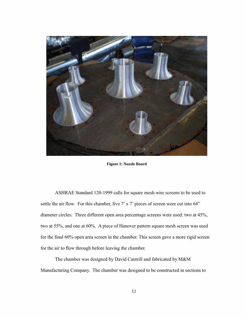
the edge of the interface to complete the seal. Figure 1 shows the nozzle board after

completion.

11

Figure 1: Nozzle Board

ASHRAE Standard 120-1999 calls for square mesh wire screens to be used to

settle the air flow. For this chamber, five 7’ x 7’ pieces of screen were cut into 64”

diameter circles. Three different open area percentage screens were used: two at 45%,

two at 55%, and one at 60%. A piece of Hanover pattern square mesh screen was used

for the final 60% open area screen in the chamber. This screen gave a more rigid screen

for the air to flow through before leaving the chamber.

The chamber was designed by David Cantrill and fabricated by M&M

Manufacturing Company. The chamber was designed to be constructed in sections to

12

allow the user to fix problems in the chamber without dismantling the whole chamber.

Each section of the chamber was made from sixteen (16) gauge cold rolled galvanized

steel and was painted with a black latex enamel to give the chamber a corrosion resistant

outer layer. The chamber was cylindrical with an inner diameter of 60”. Two inch high,

¼” thick steel flanges were attached to each of the sections to allow for the sections to be

attached to each other. A circular ¼” bolt hole pattern was cut into each flange utilizing

12 holes in the pattern. Each section was attached to the next section of the chamber

using ¼” hex head bolts and ¼” nuts. At each flange-flange interface, a flat circular

piece of red silicon gasket was used to seal the chamber. The nine sections used to

construct the chamber were as follows: two endcap-ring sections, three 36” long

cylindrical sections, four 6” long cylindrical sections and one 36” cylindrical section

with a door cutout. For the endcap-ring sections, a 30” diameter ring was attached to a

60” diameter endcap. The endcap-ring section allows various transition pieces to be

attached at the entrance and exit of the chamber. The cylindrical section with a door

cutout was designed with an interface fabricated into the section for a door to be placed

in this section. This door was used to access the nozzles after the chamber was

completely together.

The chamber was constructed in the following order (from entrance to exit):

entrance endcap-ring section, 36” long section, 45% open area wire mesh screen, 6” long

section, 55% open area wire mesh screen, 6” long section, 60% open area wire mesh

screen, 36” long section, nozzle board, cylindrical section with door cutout, 45% open

area wire mesh screen, 6” long section, 55% open area wire mesh screen, 6” long

13

section, 60% open area Hanover pattern screen, 36” long section, and an exit endcap-

ring section. After bolting the chamber sections together, silicon caulking was placed

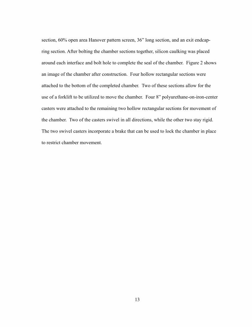
around each interface and bolt hole to complete the seal of the chamber. Figure 2 shows

an image of the chamber after construction. Four hollow rectangular sections were

attached to the bottom of the completed chamber. Two of these sections allow for the

use of a forklift to be utilized to move the chamber. Four 8” polyurethane-on-iron-center

casters were attached to the remaining two hollow rectangular sections for movement of

the chamber. Two of the casters swivel in all directions, while the other two stay rigid.

The two swivel casters incorporate a brake that can be used to lock the chamber in place

to restrict chamber movement.

14

Figure 2: Completed Chamber

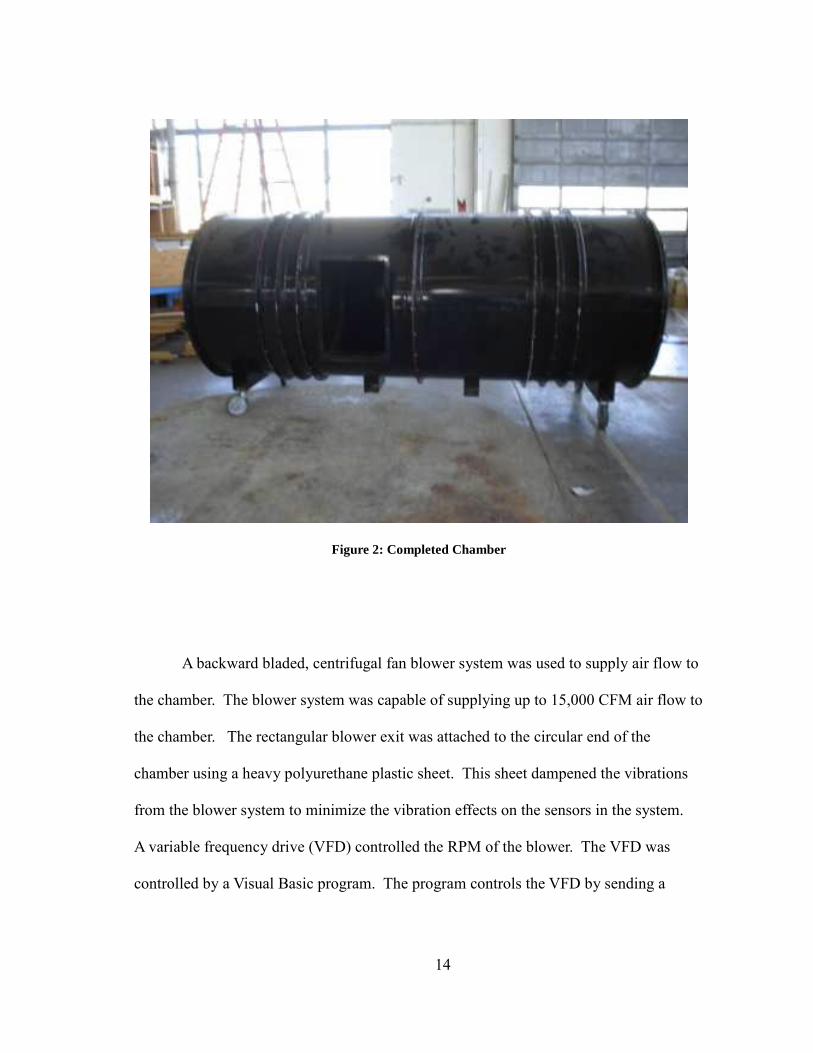
A backward bladed, centrifugal fan blower system was used to supply air flow to

the chamber. The blower system was capable of supplying up to 15,000 CFM air flow to

the chamber. The rectangular blower exit was attached to the circular end of the

chamber using a heavy polyurethane plastic sheet. This sheet dampened the vibrations

from the blower system to minimize the vibration effects on the sensors in the system.

A variable frequency drive (VFD) controlled the RPM of the blower. The VFD was

controlled by a Visual Basic program. The program controls the VFD by sending a

15

voltage to the VFD which is proportional to the RPM of the blower. Figure 3 shows the

blower and the VFD used.

Figure 3: Blower (left) and VFD (right)

A twenty (20) gauge galvanized steel duct transition piece was mounted to the

exit of the chamber. This transition piece gradually changed the diameter of the system

from the 30” diameter ring to the diameter of the duct to be tested. The slope of the

transition cannot be greater than 7.5° as specified in ASHRAE Standard 120-1999. For

this study, three transition pieces were manufactured with exit diameters of 12”, 14” and

16”.

16

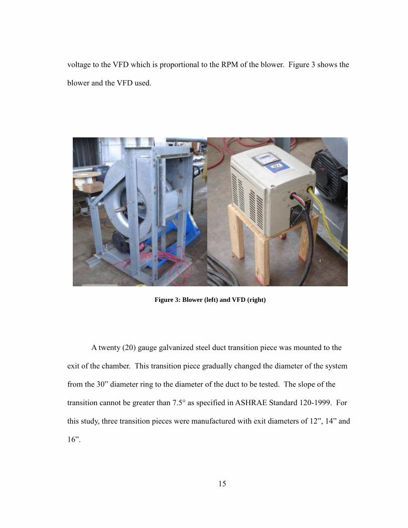
The duct used for testing sat upon duct supports. The duct supports were made

from 2” x 4” pine pieces cut to length. The supports consisted of three sections: a top

section and two legs. The top section measured 6’ in length and 24.5” in width. Starting

from the front, 2” x 4” pieces are placed 24” apart on centers. Five lengths of 2” x 4”

pine were used to make each leg. Each side of the leg used one 30” long piece and one

18” long piece. Two sets of three holes were drilled into each of the pieces used for the

side of the leg. These holes allowed the support to be moved up or down to allow the

duct to match the height of the transition piece attached to the chamber. An 18.5” long

piece of 2” x 4” attached perpendicularly to each of the 30” long pieces to provide

rigidity for the leg. The 30” and 18” long pieces attached to each other using a carriage

bolt placed through one of the holes in each piece. Each leg assembly attaches to the top

section with 2” wood screws. Twelve support sections were constructed to match the

longest length of duct to be tested. Figure 4 shows a support without the lower legs

attached.

17

Figure 4: Duct Support without Lower Legs

The rigid duct testing entrance and exit sections are fabricated before any testing

occurs. The entrance and exit section lengths do not change during the testing of a duct

diameter. The entrance section was constructed from galvanized sheet metal duct. The

length of the section must be greater than ten duct diameters to be in compliance with

ASHRAE Standard 120-1999. The exit section was constructed from galvanized sheet

metal duct with a length greater than four duct diameters. An entrance and exit section

was constructed for each diameter of duct tested.

18

CHAPTER IV

ELECTRONICS/SENSOR SETUP

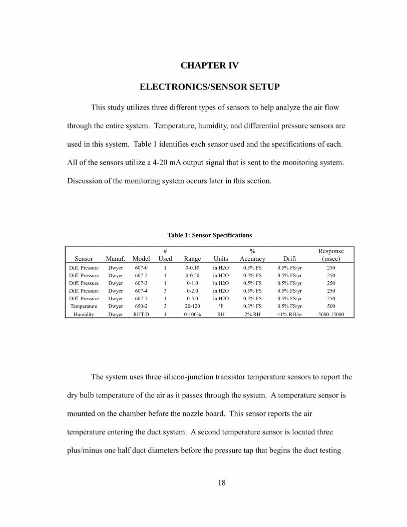
This study utilizes three different types of sensors to help analyze the air flow

through the entire system. Temperature, humidity, and differential pressure sensors are

used in this system. Table 1 identifies each sensor used and the specifications of each.

All of the sensors utilize a 4-20 mA output signal that is sent to the monitoring system.

Discussion of the monitoring system occurs later in this section.

Table 1: Sensor Specifications

Sensor Manuf. Model #

Used Range Units %

Accuracy Drift Response

(msec) Diff. Pressure Dwyer 607-0 1 0-0.10 in H2O 0.5% FS 0.5% FS/yr 250 Diff. Pressure Dwyer 607-2 1 0-0.50 in H2O 0.5% FS 0.5% FS/yr 250 Diff. Pressure Dwyer 607-3 1 0-1.0 in H2O 0.5% FS 0.5% FS/yr 250 Diff. Pressure Dwyer 607-4 3 0-2.0 in H2O 0.5% FS 0.5% FS/yr 250 Diff. Pressure Dwyer 607-7 1 0-5.0 in H2O 0.5% FS 0.5% FS/yr 250 Temperature Dwyer 650-2 3 20-120 °F 0.3% FS 0.5% FS/yr 500

Humidity Dwyer RHT-D 1 0-100% RH 2% RH <1% RH/yr 5000-15000

The system uses three silicon-junction transistor temperature sensors to report the

dry bulb temperature of the air as it passes through the system. A temperature sensor is

mounted on the chamber before the nozzle board. This sensor reports the air

temperature entering the duct system. A second temperature sensor is located three

plus/minus one half duct diameters before the pressure tap that begins the duct testing

19

section. The third temperature sensor is located three plus/minus one half duct diameters

after the pressure tap that ends the duct testing section. These two sensors report the

entrance and exit temperature of the air in the test section, respectively.

The humidity sensor used in this system reports the relative humidity value.

Although the sensor has the ability to report both humidity and temperature, for this

study, the sensor reports only humidity. The sensor uses a capacitance effect polymer

element.

The system utilizes multiple differential pressure sensors to report the static

pressures at multiple spots along the system. These pressure sensors use a diaphragm in

the sensor housing to report the pressure readings. This diaphragm deflects under

pressure which sends a voltage from the sensor to the monitoring system in proportion to

the amount of deflection. The first use of the sensors measures the differential pressure

across the nozzle board. The user uses this pressure reading to determine the amount of

air flowing into the ducts. Three sensors are used to find the pressure across the nozzles.

One sensor reads the pressure on the entrance side of the nozzles. This sensor reads the

difference between the moving air static pressure and the standard air in the area of

testing. Another sensor reads the same type of difference, but on the exit side of the

nozzles. The third sensor reports the difference in pressure between the entrance side and

the exit side of the nozzles. For the duct testing section, a similar system is used to

measure the pressure loss through the test section. One sensor measures the difference in

the static pressure entering the section against the standard air in the testing area.

20

Another sensor reads a same differential pressure at the exit of the test section. A third

sensor measures the difference in the entrance static pressure and the exit static pressure.

The system uses piezometer rings attached to the pressure sensor by a length of

silicon tubing to measure the pressure in the system. The piezometer rings used follow

the specifications for piezometer rings in ASHRAE Standard 120-1999, Section 6.2.

Section 6 of ASHRAE Standard 120-1999 also shows a figure of a piezometer as an

example. This device functions as an averaging device for the four static pressure

readings where installed. The monitoring system uses this one averaged value as the

reported pressure reading. The piezometer ring is made of silicon tubing and mounts to

the duct using four pressure taps. ASHRAE 120-1999, Section 6.3 and Figure 1 in

Section 6 give the acceptable dimensions needed. The taps were made from 24 gauge

copper plate and ¼” outer diameter copper tubing. The copper plate is cut into sixteen

3” by 3” square pieces. Sixteen 1 inch pieces are cut from the copper tubing. The

copper tubing pieces are soldered to the copper plate in the center of one side. After

soldering the assembly is quenched in a water bath to cool and harden the soldered area.

Once the assembly is cooled, a 1/8” hole is drilled through the copper plate. The center

of the drilled hole is drilled at the center of the copper tube. The process repeats until all

sixteen assemblies are finished. Before mounting the taps to the duct, four 3/32” holes

are drilled into the duct at four equidistant spots around the duct. These four holes must

be in a single plane. The tap assemblies mount to the duct using a layer of silicon

caulking. The hole in the duct must line up with the tubing. The plate of the tap

assembly contours to the shape of the duct. To secure the tap to the duct and to seal the

21

tap, aluminum duct tape is used. Once the taps are mounted to the duct, the piezometer

ring attaches to each of the four taps. The single output of the ring attaches to the

pressure sensor with a length of ¼” silicon tubing. The temperature sensors also mount

using silicon caulking and aluminum duct tape. Figure 5 gives an example of the

piezometer ring and temperature sensor mounted to the duct.

Figure 5: Piezometer Ring (left) and Temperature Sensor (right) Mounted

All of the sensors attach to the data acquisition (DAQ) system through a DAQ

board. A piece of wire connects the negative terminal of the sensor to a designated

channel of the DAQ board. A wire connects the next associated channel to the negative

22

terminal of the 12 volt – 1 amp power supply. To attach all of the sensors to the one

negative power supply terminal, a piece of wire runs from the negative power supply

terminal to a wing nut. The wires from the associated channels for each sensor run to

this same wing nut. This cluster of wiring in the wing nut allows for multiple

connections to the one power supply terminal. The positive side of the loop uses the

same method with the wing nut. A single wire comes from the positive power supply

terminal and meets with the wires from the positives of each sensor at the wing nut. A

250Ω (.05%) precision resistor placed between the two channels on the DAQ board

completes the sensor loop for each sensor. This resistor converts the current output of

the sensor to a voltage input to the DAQ system. A NEMA 1 case houses the pressure

sensors, wiring, and DAQ board. The case protects its contents from dust and other

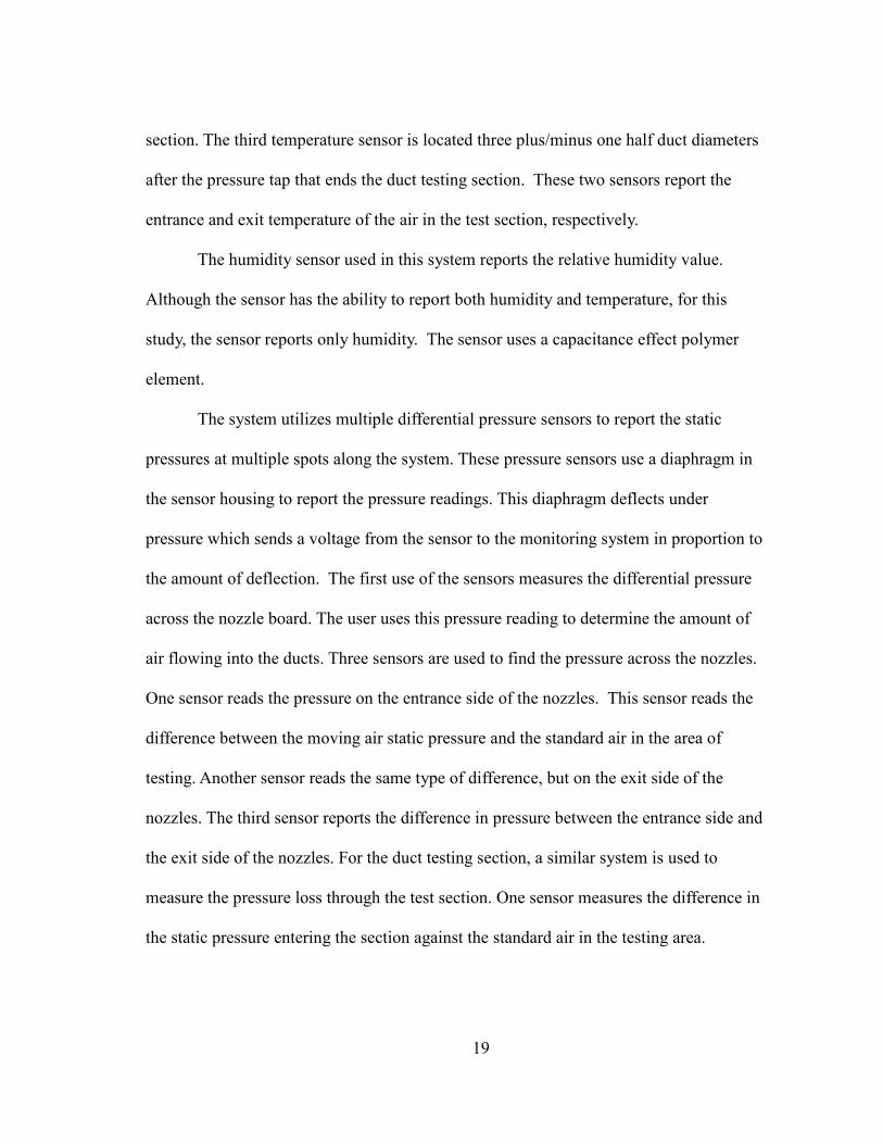
contaminants. Figure 6 shows the sensor wiring diagram. Figure 7 shows a picture of

the pressure sensors and Figure 8 shows the DAQ board wiring. The DAQ board

connects to a DAQ card mounted in a computer. The board sends the voltage readings to

the card which the computer uses to report the readings to the user.

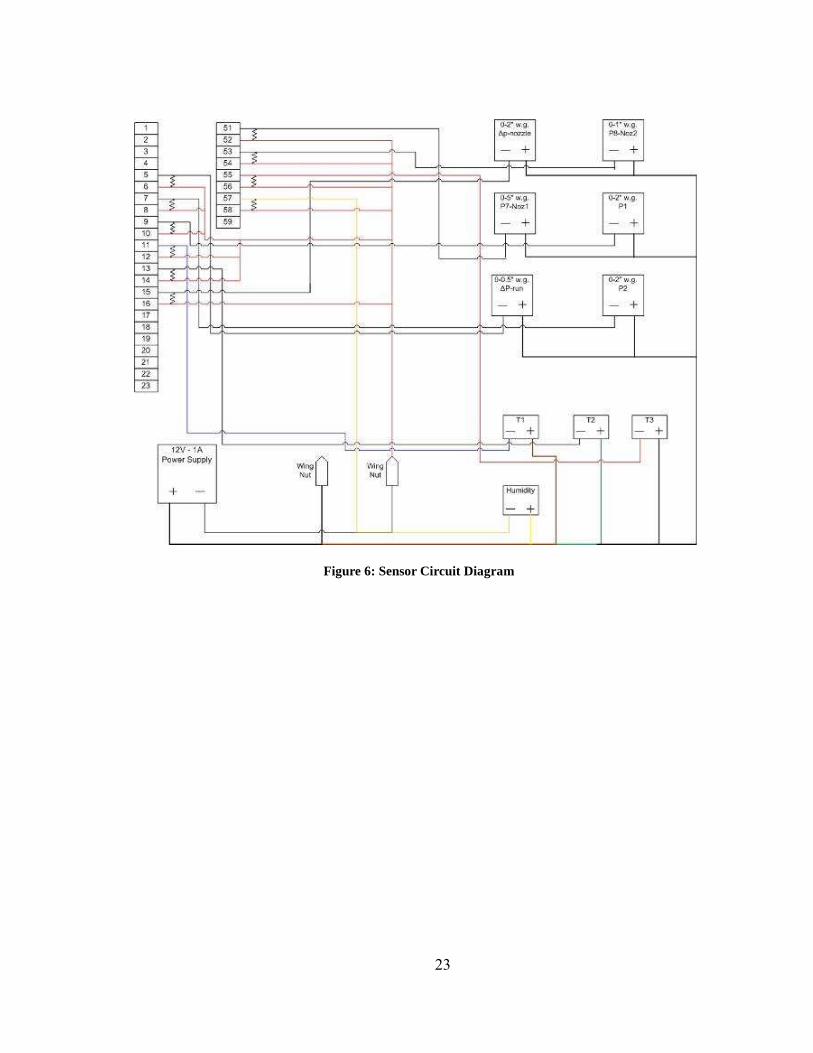
23

Figure 6: Sensor Circuit Diagram

24

Figure 7: Differential Pressure Sensor Array

25

Figure 8: DAQ Board Wiring

26

CHAPTER V

VISUAL BASIC MONITOR, FLOW CALCULATOR, AND TEST

VERIFICATION

To control the measurements and operation of the system, a Visual Basic

program was written. Figure 9 gives an example screenshot of the monitor window

which gives the user control of the system.

Figure 9: Visual Basic Monitor Window

27

The program setup allows for the VFD to be controlled with a slider. The

movement of this slider changes the voltage sent to the VFD. The first column of the

program allows for each sensor to be given a name. This allows the user to easily

identify what each sensor outputs. The channel in which the sensor connects to the DAQ

board goes into the second column. The third column identifies the minimum voltage

outputted by the sensor. Because all of the sensors are on a 4-20 mA circuit with a 250Ω

resistor, every sensor has a minimum voltage value of 1. The next column contains the

maximum voltage output of the sensor. For the same reason as the minimum voltage,

this voltage is 5. The scalar column allows the user to input the factor which scales the

voltage value to give a true unit reading. For pressure sensors, the maximum pressure

value of the sensors is inputted in the column. For the temperature sensors, 1 is inputted.

For the humidity sensor, 100 is inputted. The 100 scalar converts the RH value from a

decimal to a percentage. The next column reports the voltage outputted from the sensor

itself. The final column gives the value outputted by the sensor in a true unit form

except for the temperature sensors. For pressure the true unit is in H2O and for humidity

it is %RH. The top button on the right of the monitor window allows the user to start

and stop the monitor window’s real-time sensor reporting. The next button exports the

reported real-time values to an Excel spreadsheet for storage until data analysis.

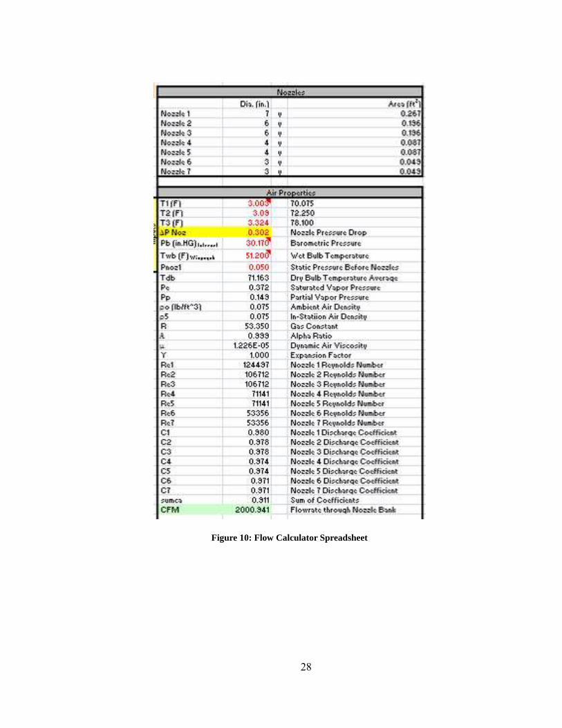
An important tool used in the study is the flow calculator spreadsheet. This

spreadsheet calculates the pressure drop across the nozzles necessary to achieve a certain

air flow rate. Figure 10 shows an example of the spreadsheet used.

28

Figure 10: Flow Calculator Spreadsheet

29

The top box of this spreadsheet contains information about the nozzles used in

each test. A “Y” is placed in the appropriate column for each nozzle that is open for the

test. The next box contains the information concerning the air flow through the system.

The user inputs values for the three temperature sensors, the barometric pressure, the

static pressure before the nozzles, the wet bulb temperature, and the differential pressure.

The three inputted temperature values average to give the dry bulb temperature. The

spreadsheet uses these values in conjunction with formulas located in ASHRAE

Standard 120-1999, Section 9 to find and output an air flow rate. The spreadsheet also

reports each of the values calculated and subsequently used in the calculation of the air

flow rate. From this spreadsheet, the user takes the differential nozzle pressure and uses

it in conjunction with the monitor window to control the VFD.

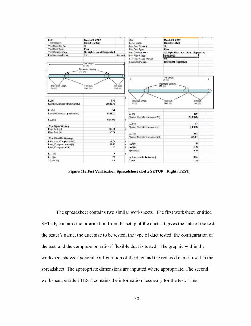
The next tool used in this study comes in the form of the test verification

spreadsheet (TVS). This spreadsheet contains all of the descriptive information about

each test. Figure 11 shows an example of the test verification spreadsheet.

30

Figure 11: Test Verification Spreadsheet (Left: SETUP - Right: TEST)

The spreadsheet contains two similar worksheets. The first worksheet, entitled

SETUP, contains the information from the setup of the duct. It gives the date of the test,

the tester’s name, the duct size to be tested, the type of duct tested, the configuration of

the test, and the compression ratio if flexible duct is tested. The graphic within the

worksheet shows a general configuration of the duct and the reduced names used in the

spreadsheet. The appropriate dimensions are inputted where appropriate. The second

worksheet, entitled TEST, contains the information necessary for the test. This

31

worksheet contains the basic dimensions from the SETUP worksheet. This worksheet

differs from the other by the addition of the flow range, the flow range interval, and the

applicable pictures taken for the test. A TVS is made for each test configuration that is

tested. This allows individuals to recreate the tests if necessary.

32

CHAPTER VI

AIRFLOW EQUATIONS

The air flow rates used in the system were determined by measuring the static

pressure loss across flow nozzles mounted on a nozzle board in the chamber. The flow

calculator spreadsheet discussed in Chapter 5 was used to calculate the desired air flow

rate using the measured static pressure drop across the nozzles. All equations used in the

flow calculator spreadsheet are taken from ASHRAE Standard 120-1999, Section 9. The

following are the user inputs into the flow calculator spreadsheet and the equations used

to calculate air flow rates from the static pressure drop across the nozzles.

Inputs

The following variables are either measured using the air flow test setup or are

visually determined. IP units shown in parenthesis. SI units shown in brackets.

Diai Diameter of each nozzle used in test. (in) [cm]

Ani Area of each nozzle used in test. (ft2) [m2]

∆Pnoz Measured static pressure drop through nozzle bank. (in-H2O) [Pa]

Tdb Dry bulb temperature of air within test duct. Calculated as average of T1

and T2. (°F) [°C]

Pb Barometric pressure. Taken from weather data for Easterwood Airport,

which is located 8 miles from the test location. (in-Hg) [kPa]

33

Twb Wet bulb temperature of air within test system. Calculated using

psychrometric properties for air with inputs of dry bulb temperature (Tdb)

and relative humidity (RH) from monitor program. (°F) [°C]

Pnoz1 Static pressure in in-H2O recorded before nozzle bank (in-H2O) [Pa]

Equations

Pe Saturated Vapor Pressure (6.1)

(IP) 41.0)10*59.1()10*96.2( 223 ++= −−wbwb TT )20( Hin −

(SI) 692.0)10*86.1()10*25.3( 223 ++= −−wbwb TT )(kPa

Pp Partial Vapor Pressure (6.2)

(IP) 2700

))(( wbambbe

TTPP

−−= )20( Hin −

(SI) 1500

))(( wbambbe

TTPP

−−= )(kPa

ρo Ambient Density of Air (6.3)

(IP) )67.459(35.53)378.0(75.70

+−

=amb

pb

T

PP )( 3ft

lb

(SI) )2.273(287.0

)378.0(−

−=

amb

pb

T

PP )( 3m

kg

34

ρ5 Density of air within chamber (6.4)

(IP)

+

++

=b

bnoz

db

ambo P

PP

T

T

63.1363.13

67.45967.459 1ρ )( 3ft

lb

(SI)

+

++

=b

bnoz

db

ambo P

PP

T

T

10001000

2.2732.273 1ρ )( 3m

kg

Α Alpha ratio (6.5)

(IP)

+∆

−=b

noz

PP

P

63.131

5

(SI)

+∆

−=b

noz

PP

P

10001

5

µ Dynamic air viscosity (6.6)

(IP) 65 10)018.011( −+= T

)*

(sft

lbm

(SI) 65 10)048.023.17( −+= T )*( sPa

Yn Expansion factor (6.7)

(IP) 5.0286.0

43.1

115.3

−−=

ααα

35

(SI) 5.0286.0

43.1

115.3

−−=

ααα

Re Reynolds Number of air within chamber (6.8)

(IP) ( ) 5.0512

000,363,1 nozPd ∆

= ρ

(SI) ( ) 5.05900,70 nozPd ∆= ρ

Ci Discharge Coefficient (6.9)

(IP) dRe

1000653.09965.06

−=

(SI) Re1000653.09965.0

6

−=

ΣCa Sum of coefficients

ii CAnCAnCAn *....** 2211 +++= (6.10)

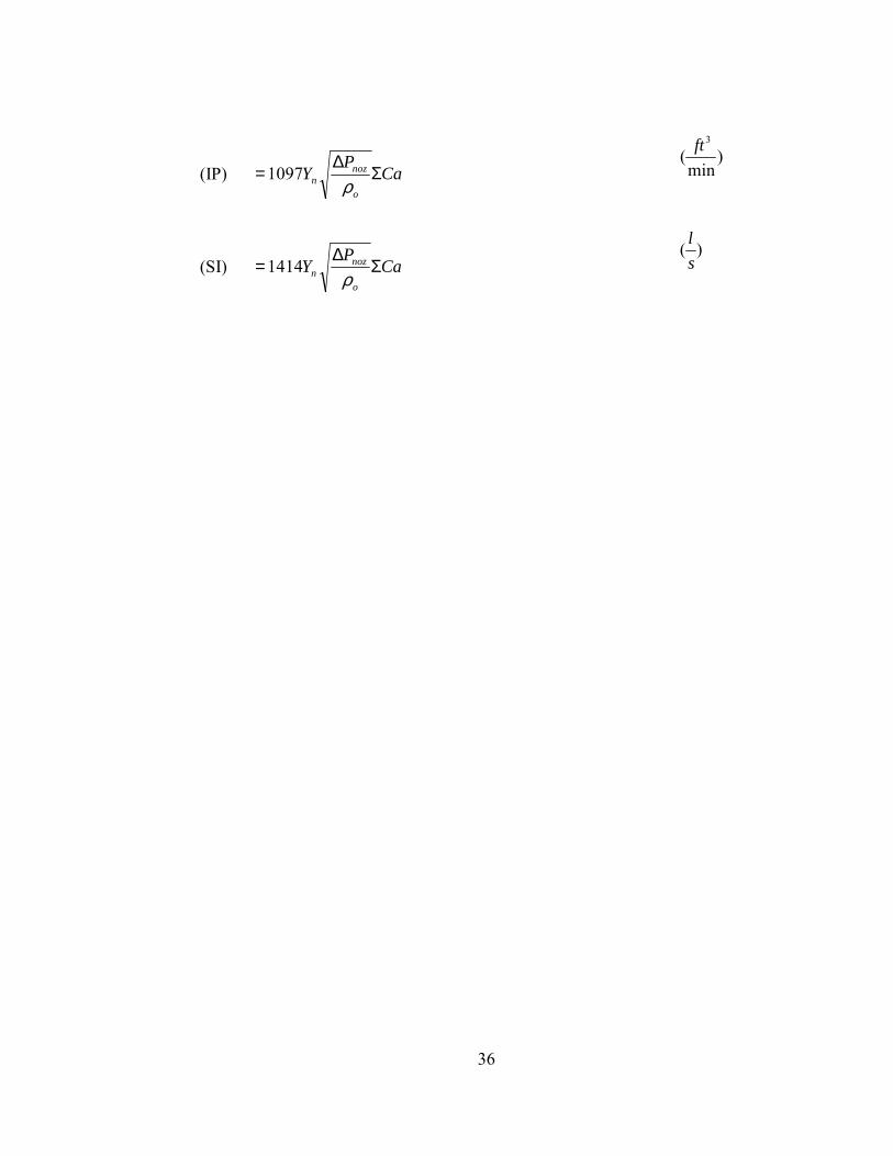
CFM Volumetric flow rate (6.11)

36

(IP) CaP

Yo

nozn Σ

∆=

ρ1097

)min

(3ft

(SI) CaP

Yo

nozn Σ

∆=

ρ1414

)(s

l

37

CHAPTER VII

TEST METHODOLOGY

Nozzle Board Leak Test

Prior to assembly of the complete test setup, the nozzle board requires leak

testing to ensure that leakage from seals and nozzles does not exceed allowable

tolerances. The leak testing procedure is outlined in the following steps:

1. Leak testing is to occur on a monthly basis.

2. Seal blower end of chamber.

a. Use object cut to fit exit diameter.

b. Apply blue painter’s tape to completely seal opening.

3. Open door to outlet side of nozzle board.

4. Seal all nozzles inside chamber.

a. Use nozzle caps to cover each nozzle outlet.

b. Apply tape to junction where cap and nozzle intersect with blue

painter’s tape to ensure a tight seal.

5. Attach air hose from flow measurement device (shown in Figure 12) to

barbed air hose connection on chamber (shown in Figure 13).

38

Figure 13: Barbed Air Hose Connection

Figure 12: Flow Measurement Device

39

6. Attach other end of flow measurement device to hose connected to air

supply (air compressor) using the quick release connection.

7. Open Monitor Window Program from computer desktop.

8. Press “Scan” button.

9. Turn knob on flow measurement device until the differential pressure

sensor located on the inlet side of the nozzle board displays a value of

approximately 0.100” H2O.

10. Once the pressure reaches approximately 0.100” H2O, record the height

of the top of the red ball within the flow measurement device cylinder.

11. This value is equivalent to the amount of air flow that is entering the

system to maintain the described pressure. This value also represents the amount

of leakage in the section tested.

12. This value is displayed in units of cubic feet per hour of Argon (CFH).

13. This value needs to be converted to cubic feet per hour of air.

14. A value of 1 is used to convert from cubic feet per hour of Argon to cubic

feet per hour of air, given that the precise conversion factor from Argon to Air is

0.999.

15. The value is further converted to units of cubic feet per minute of air

(CFM) using the conversion factor of 1 CFH = 60 CFM.

16. ASHRAE Standard 120 - 1999 does not state a maximum amount of

leakage across the nozzle board.

40

17. Air leakage rates less than 1 CFM shall be considered acceptable for

testing purposes, based on rule of thumb criteria.

18. There is an inversely proportional relationship between the air leakage

rate and the accuracy of future readings during duct testing and thus lower

leakage rates are desirable.

19. If the tested leakage value is below the maximum allowable leakage rate,

testing may begin.

20. If the leakage is found to be greater than the maximum acceptable rate,

sources of air leakage should be identified and sealed until the measured air

leakage for the nozzle board falls below the maximum allowable rate.

Preassembly of Duct

Upon completion of the nozzle board leak test, the remainder of the test

apparatus can be assembled. The preassembly of the duct only needs to be done when

ready to test a new duct diameter. First, select the sheet metal transition piece that

changes the duct diameter from the 30” diameter of the endcap-ring piece to the

diameter of the duct to be tested. Slide the transition piece onto the collar of the

chamber and screw the transition piece and collar together with self-tapping sheet metal

screws. Using aluminum duct tape, tape the lateral joint where the collar and transition

piece meet. Smooth out the tape to remove any air bubbles in the tape. Next, apply

another layer of tape to this lateral joint staggered with the first layer and smooth out the

tape to remove any air bubbles. Then, slide the premade duct entrance section for the

41

correct duct diameter onto the end of the transition piece. Tape the lateral joint using the

same procedure used to tape the transition piece to the endcap-ring.

For rigid duct testing, slide the necessary length of rigid duct required for testing

(minimum of 25 diameters) and tape each lateral joint in the manner used above. For

flexible duct testing, attach the appropriate length of flexible duct required for testing

(minimum 25 diameters) to the end of the entrance section. Tape the end of the plastic,

flexible duct material to the end of the rigid entrance section. Figure 14 shows an

example of the flexible duct connected to the entrance section.

Figure 14: Flexible Duct – Entrance Section Joint

42

If multiple lengths of flexible duct are required, use a sheet metal collar to

connect the lengths end to end and tape them onto the collar using aluminum tape. Next,

fully stretch the entire length of flexible duct and mark equal, one foot sections. After

placing the last length of duct (rigid or flexible) for testing, attach the premade duct exit

section of the correct diameter. Tape the lateral joint in the manner used above.

System Leak Testing

After completing the preassembly of the duct, the system needs to be leak tested.

The leak test considers the chamber, transition piece, and duct sections as one complete

system. This leak testing follows a similar procedure as the nozzle board leak test as

follows:

1. This test should be done with each change of configuration.

a. Examples are rigid testing and flexible testing

b. Done any time there is a break in the setup.

2. Seal blower end of chamber and duct exit end of chamber.

a. Use object cut to diameter of exit.

b. Tape with blue painter’s tape to ensure it is sealed.

3. Make sure chamber door is closed and sealed.

4. Attach air hose from flow measurement device (shown in Figure 12) to

barbed air hose connection on chamber (shown in Figure 13).

43

5. Attach other end of flow measurement device to hose connected to air

supply (air compressor) using the quick release connection.

6. Open Monitor Window Program from desktop.

7. Press “Scan” button.

8. Turn knob on flow measurement device until all pressure sensors are

displaying a value of about 0.100” H2O.

9. Once pressures reach about 0.100” H2O, record the height of the top of

the red ball in the cylinder of the flow measurement device.

10. This value is the amount of air flow that is entering the system to

maintain the described pressure. This value also equals the amount of leakage in

the system.

11. This value is displayed in units of cubic feet per hour of Argon (CFH).

12. This value needs to be converted to cubic feet per hour of air.

13. Because the multiplier to convert from Argon to air is 0.999, the

multiplier used is 1.

14. The value is converted to units of cubic feet per minute of air (CFM)

using the relationship of 1 CFH = 60 CFM

15. ASHRAE Standard 120 - 1999 requires that the maximum amount of

leakage in the system is 0.5% of the minimum air flow that will be tested.

44

16. For example, if the lowest air flow to be tested is 200 CFM, the

maximum amount of leakage for the system is 1 CFM.

17. If the tested leakage value is within the acceptable range, testing may

begin.

18. Otherwise leak sources should be identified and sealed until the standard

leak rate is no longer exceeded.

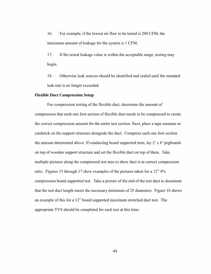
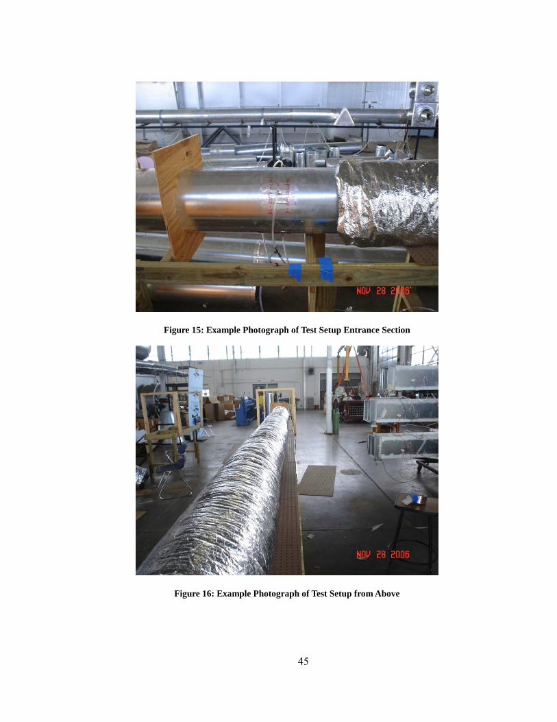
Flexible Duct Compression Setup

For compression testing of the flexible duct, determine the amount of

compression that each one foot section of flexible duct needs to be compressed to create

the correct compression amount for the entire test section. Next, place a tape measure or

yardstick on the support structure alongside the duct. Compress each one foot section

the amount determined above. If conducting board supported tests, lay 2’ x 8’ pegboards

on top of wooden support structure and set the flexible duct on top of them. Take

multiple pictures along the compressed test area to show duct is at correct compression

ratio. Figures 15 through 17 show examples of the pictures taken for a 12” 4%

compression board supported test. Take a picture of the end of the test duct to document

that the test duct length meets the necessary minimum of 25 diameters. Figure 18 shows

an example of this for a 12” board supported maximum stretched duct test. The

appropriate TVS should be completed for each test at this time.

45

Figure 15: Example Photograph of Test Setup Entrance Section

Figure 16: Example Photograph of Test Setup from Above

46

Figure 17: Example Photograph of Test Setup from Side

Figure 18: Example Photograph Showing Length of Test Section

47

Operation

To start the testing process, turn on the data acquisition PC and open the Visual

Basic monitor program and the flow calculator spreadsheet. Next, determine the air flow

range to be tested. Determine which nozzles need to be used for the set of tests using the

flow calculator spreadsheet. Input an upper limit for the differential pressure and vary

the nozzles that are opened until the upper limit of the intended air flow range is given.

The author used a differential pressure of no greater than 2.5” w.g. when determining the

nozzles to be used. Once the necessary nozzles are found, open and remove the chamber

door. Place nozzle endcaps on the nozzles that will not be used. Place blue painter’s

tape around the joint where the caps and the nozzles meet to seal the nozzles. Replace

and close the chamber door ensuring an airtight seal. Next, plug the VFD into a 480V

outlet and turn the outlet on. Press the RUN MODE button on the VFD until the green

“manual” light lights up. Next, press the RUN button on the VFD. This will cause the

blower to start rotating at a low RPM. Figure 19 shows the interface of the VFD and the

buttons used above.

48

Figure 19: VFD Interface

Next, press the “Scan” button in the monitor window. Using the flow calculator

spreadsheet, determine the pressure drop that corresponds with the air flow rate to be

tested. Input the temperature voltage readings from the monitor window. Input the

correct nozzles used for the test. Input the barometric pressure found on the NOAA

website for Easterwood Airport in College Station, TX:

(http://www.srh.noaa.gov/ifps/MapClick.php?CityName=College+Station&state=TX&si

te=HGX). Using the dry bulb temperature given in the calculator and the humidity value

49

from the monitor window, calculate the wet bulb temperature using a psychrometric

computer program. This program is a simple psychrometric calculation program that

determines wet bulb temperature using dry bulb temperature and relative humidity as

inputs. Input the wet bulb temperature from the psychrometric program into the flow

calculator spreadsheet. Input values for the nozzle differential pressure until the air flow

rate is at the desired flow rate to be tested.

Using the nozzle differential pressure value from the flow calculator spreadsheet,

move the VFD slider bar on the monitor window until the value for the differential

pressure across the nozzles on the monitor matches the value of the nozzle differential

pressure from the flow calculator spreadsheet. Once the value of the nozzle differential

pressure becomes stable (varies less than ±0.005” w.g.), press the “Export” button. This

opens an Excel spreadsheet and exports sensor values for each time step. For this study,

the time step used was one second. After the required number of data points has been

taken (50), press the “Stop” button that used to read “Export” in the monitor window.

This button will return to reading “Export.” Press the “Save As” button and name the

file and place it in the appropriate folder of the PC’s hard drive. Next, close the Excel

file. Repeat the process beginning with the flow calculator for the next flow rate to be

tested. Repeat until all flow rates in the desired range are tested. If testing rigid duct,

this ends the testing procedure. For flexible duct testing, the compression amount of the

duct needs to be changed to the next compression to be tested. Then, the process is

repeated beginning with the test flexible duct test setup section above.

50

CHAPTER VIII

ANALYSIS METHODOLOGY

After the data collection phase ended, the data was analyzed and trended. To

begin the analysis, the Excel spreadsheet that contains the lowest flow rate for the

compression ratio tested was opened. The data points for each column of data which

contained approximately 50 values were averaged to one value for each column. The

spreadsheet was resaved to include the averaged values. Figure 20 provides an example

of the averaged value row. The next flow rate spreadsheet in the range was opened and

averaged as above. This process was repeated until each flow rate in the range was

averaged.

Another spreadsheet was created to contain the averaged values from each set of

approximately 50 flow rate measurements collected in the range tested. The spreadsheet

contains the averaged data. Figure 8-2 shows the setup of this spreadsheet. The first two

rows of the spreadsheet contain the conversion factors used to convert the pressure drop

across the test section and the air flow rate from IP units to SI units. These spreadsheets

contain data in both units. The fourth row includes the length of duct tested associated

with the test range being analyzed. The fifth row contains the length of rigid sheet metal

duct contained in the total test length. The seventh row of the spreadsheet contains the

sensor names, flow rate in both sets of units, and the differential pressure across the test

section in both IP and SI units. Rows 8 and higher contain the averaged and analyzed

data in ascending order starting with the lowest flow rate in the test range. Table 2

describes the organization of columnar data from the spreadsheet in Figure 21.

51

Figure 20: Example of Averaged Row

52

Table 2: Analysis Spreadsheet Column Descriptions

Column Value Comment

A Blank

B CFM Air flow rate in IP units

C DP-100 Differential pressure drop per 100 feet of duct in IP units The value of this column is calculated by taking the differential pressure measured across the test section and subtracting the calculated pressure drop across the rigid length.

D L/s Airflow rate in SI units

E Pa/m Differential pressure drop in SI units

F P1 Static pressure measurement at entrance of test section

G DP-.5 Differential pressure measurement across test section with 0.5 in wg maximum sensor

H DP-.1 Differential pressure measurement across test section with 0.1 in wg maximum sensor

I P2 Static pressure measurement at exit of test section

J P7-Noz 1 Static pressure measurement at entrance of nozzle bank

K P5-DP Noz Differential pressure across nozzle bank

L P8-Noz 2 Static pressure measurement at exit of nozzle bank

M T1 Voltage reading of temperature probe at entrance of test section

N T2 Voltage reading of temperature probe at exit of test section

O T3 Voltage reading of temperature probe at airflow chamber

P Humidity Humidity reading in airflow chamber

Q Blank

R Rigid-100 Differential pressure drop per 100 feet of rigid duct in IP units

S Rigid Differential pressure drop per length of rigid duct in IP units

53

Figure 21: Example of Analysis Spreadsheet

After the analysis spreadsheet has been completely filled in, a chart was created

in Microsoft Excel to describe the flow rate as a function of pressure drop per unit

length. The “Scatter with only Markers” type of chart was used for the analysis. The

first data series contains data in IP units with the flow rate plotted on the x-axis and the

pressure drop plotted on the y-axis. The second data series contains the data in SI units.

The flow rate values were input on the x-axis and the pressure drop values were included

on the y-axis. A set of dual unit axes was then established. The IP axes were set with

the x-axis labeled as “CFM” and the y-axis labeled “H2O/100 ft.” A second set of axes

was established in the SI units with the upper x-axis labeled as “L/s” and the right side y-

axis labeled as “Pa/m”. The chart was placed in a separate worksheet within the

spreadsheet. It was necessary to plot the second data series onto a secondary set of axes

to create a dual unit chart. The process was as follows:

1. Select the second data series.

54

2. Under format data series options, select the data to be plotted on the

secondary axis. This introduces another vertical axis on the right side of the

chart. This axis was named “Pa/m”.

3. Add another horizontal axis to the chart. This axis is displayed at the top

of the chart. The name of this axis will be “L/s”.

4. Change the secondary axes’ value range to match that of the primary

axes’ values. For the vertical axis, right click on the axis and select “format

axis.” In the option windows, change the minimum and maximum values to be

the minimum and maximum values of the primary axis multiplied by the

appropriate conversion factor. Select the option that the horizontal axis crosses at

the maximum axis value.

5. Repeat step 4. for the secondary horizontal axis.

6. Select the second data series. In the data series options, select the options

for the line and markers to be none. This will “hide” the secondary data series as

it will overlap the primary data series.

7. Trend the data to show the relationship between flow rate and pressure

drop. Select the primary data series, right click to bring up the options menu and

select “add trend line.” In the add trend line window, select the trend type to be

“Power” and select the option to display the equation on the chart. Once the

trend line is plotted, right click on the trend line equation and select “format trend

line label.” In the “numbers” category, select “scientific” and set the decimal

places to four. This trend line equation gives the relationship in a mathematical

55

form of ∆p=C*Qn. In this equation, ∆p refers to the pressure drop, C is a

coefficient, Q is the flow rate, and n is an exponent. The value for n is assumed

to be 2, but it fluctuates in actual applications. Figure 22 shows an example of

the chart plotting the relationship between flow rate and pressure drop. Tables 5,

6 and 7 in Appendix A provide the approximated equation of the data for all duct

sizes and compression ratios. The table also provides the coefficient of

determination or “R-squared” value for each equation. This value shows how

“well” the curve fits the actual data.

8. The analysis spreadsheet is saved into a new folder entitled “Analysis.”

This process was repeated until each compression ratio was analyzed and

charted. The analysis data for each compression ratio was then plotted on the same

graph to allow for comparison of each compression ratio. A new spreadsheet was

created to plot the data together in a single chart. The spreadsheet’s first two rows

consist of the same conversion factors as in the individual compression ratio analysis

spreadsheet. The rest of the spreadsheet consists of the analyzed data from each tested

duct setup. The first set gives the rigid duct data. The next set gives the maximum

stretched flexible duct data. The remaining sets of data give the 4%, 15%, 30% and 45%

compression ratio data. All of the data sets are presented in both IP and SI units. Figure

23 shows an example of the spreadsheet.

56

Figure 22: Example of Analysis Chart

57

Figure 23: Example of Multiple Series Analysis Spreadsheet

The complete sets of data are then plotted in a new chart. The process for setting

up the chart is similar to the setup of the individual compression ratio chart. The chart

type remains the “Scatter with Straight Lines and Markers” chart type. For each of the

flexible duct data sets, the 45% compression plotted data is the data in SI units. The

primary axes names stay the same as before. For this chart, the legend was placed at the

bottom of the chart. Every flexible duct data set was selected and chosen to be plotted

on the secondary axes. The secondary axes’ names are the same as the individual

58

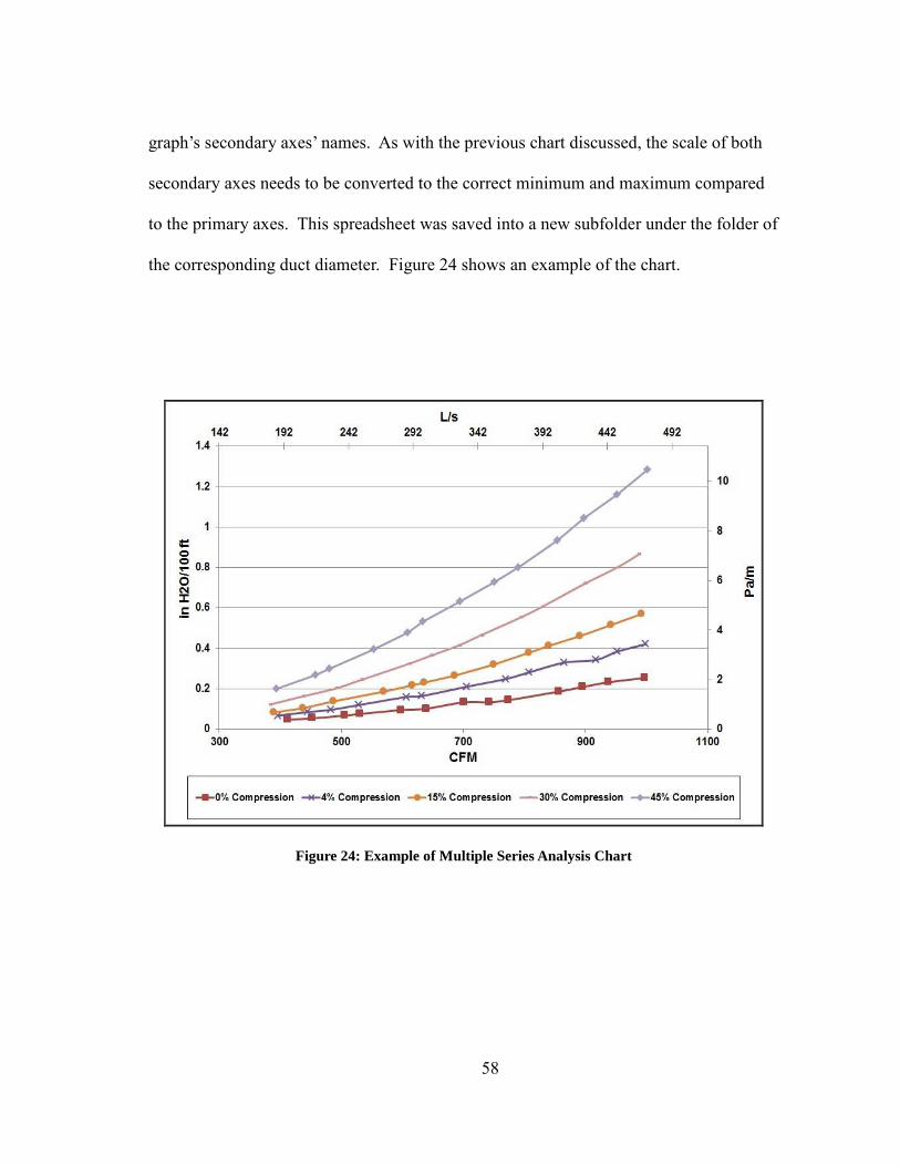
graph’s secondary axes’ names. As with the previous chart discussed, the scale of both

secondary axes needs to be converted to the correct minimum and maximum compared

to the primary axes. This spreadsheet was saved into a new subfolder under the folder of

the corresponding duct diameter. Figure 24 shows an example of the chart.

Figure 24: Example of Multiple Series Analysis Chart

*Part of data reported in this chapter is reprinted with permission from “Pressure Losses in 12”, 14” and 16” Non-Metallic Flexble Ducts with Compression and Sag” C. Culp and D. Cantrill, 2009. ASHRAE Transactions, V. 115, Pt. 1. Copyright 2009 by ASHRAE.

59

CHAPTER IX

NON-METALLIC FLEXIBLE DUCT COMPRESSION

EXPERIMENTAL RESULTS *

The results of this study are presented as the static pressure drop across the

tested duct as a function of the flow rate for each of the three duct sizes tested. The

static pressure loss through a rigid sheet metal duct is given as a baseline for comparison

in each of the graphs with pressure loss of flexible ducts of the same diameter. The

testing consisted of the following six configurations: rigid sheet metal, maximum

stretched flexible duct, 4% (natural) compressed flexible duct, 15% compressed flexible

duct, 30% compressed flexible duct, and 45% compressed flexible duct. The test flow

rates for each configuration were developed based on manufacturer recommendations.

Each comparison chart shows both the board supported and joist supported results for

each flexible duct compression. Figures 25, 26 and 27 each illustrate the variation in

pressure loss as a function of flow rate for a given duct diameter; while Figures 28

through 33 illustrate the relationship between pressure loss and flow rate for a given duct

compression.

60

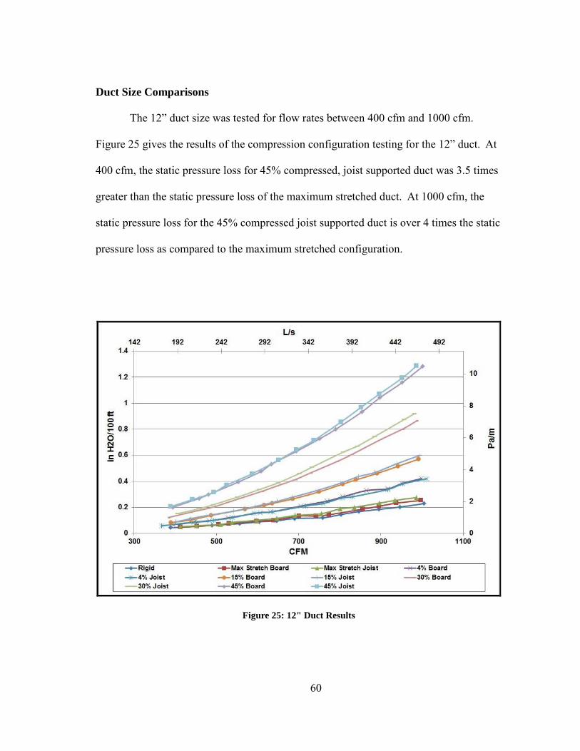
Duct Size Comparisons

The 12” duct size was tested for flow rates between 400 cfm and 1000 cfm.

Figure 25 gives the results of the compression configuration testing for the 12” duct. At

400 cfm, the static pressure loss for 45% compressed, joist supported duct was 3.5 times

greater than the static pressure loss of the maximum stretched duct. At 1000 cfm, the

static pressure loss for the 45% compressed joist supported duct is over 4 times the static

pressure loss as compared to the maximum stretched configuration.

Figure 25: 12" Duct Results

61

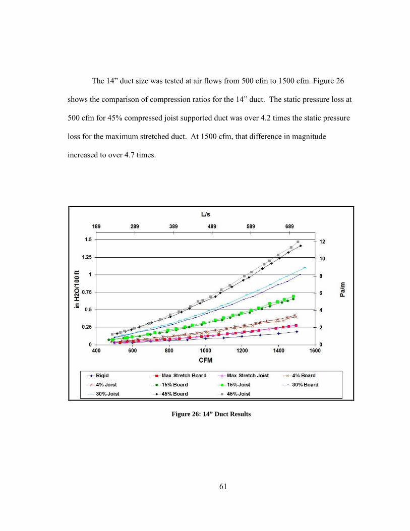
The 14” duct size was tested at air flows from 500 cfm to 1500 cfm. Figure 26

shows the comparison of compression ratios for the 14” duct. The static pressure loss at

500 cfm for 45% compressed joist supported duct was over 4.2 times the static pressure

loss for the maximum stretched duct. At 1500 cfm, that difference in magnitude

increased to over 4.7 times.

Figure 26: 14” Duct Results

62

The testing for the 16” duct was performed at an air flow rate range of 1000 cfm

to 2000 cfm. The 16” duct testing results are presented in Figure 27. The 45%

compression data for this duct size consists of two different configurations. The first

configuration used three sections of flexible duct to comply with the minimum test

length of 25 duct diameters as required by ASHRAE 120-1999. All other tests

performed on this duct size used only two sections. After performing the test and

analyzing the data, the 45% compression static pressure results were less than the 30%

compression static pressure results.

Figure 27: 16” Duct Results - 45% 3-Sections

63

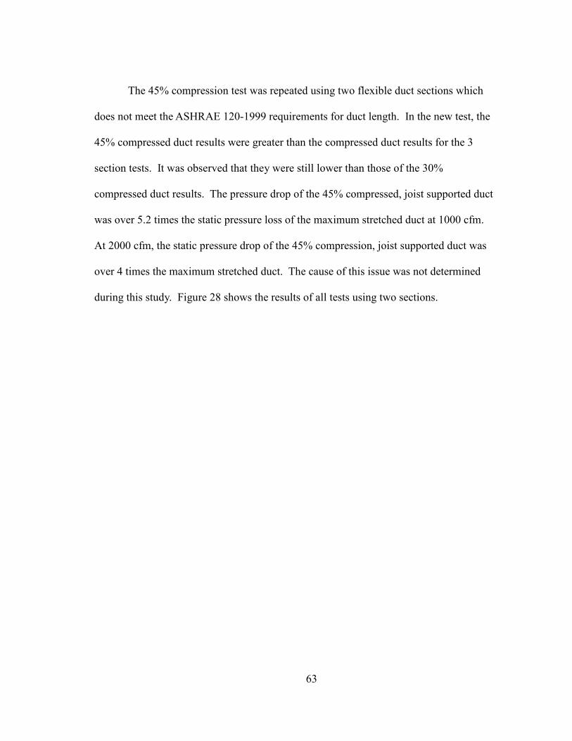
The 45% compression test was repeated using two flexible duct sections which

does not meet the ASHRAE 120-1999 requirements for duct length. In the new test, the

45% compressed duct results were greater than the compressed duct results for the 3

section tests. It was observed that they were still lower than those of the 30%

compressed duct results. The pressure drop of the 45% compressed, joist supported duct

was over 5.2 times the static pressure loss of the maximum stretched duct at 1000 cfm.

At 2000 cfm, the static pressure drop of the 45% compression, joist supported duct was

over 4 times the maximum stretched duct. The cause of this issue was not determined

during this study. Figure 28 shows the results of all tests using two sections.

64

Figure 28: 16” Duct Results - 45% 2-Sections

Compression Comparisons

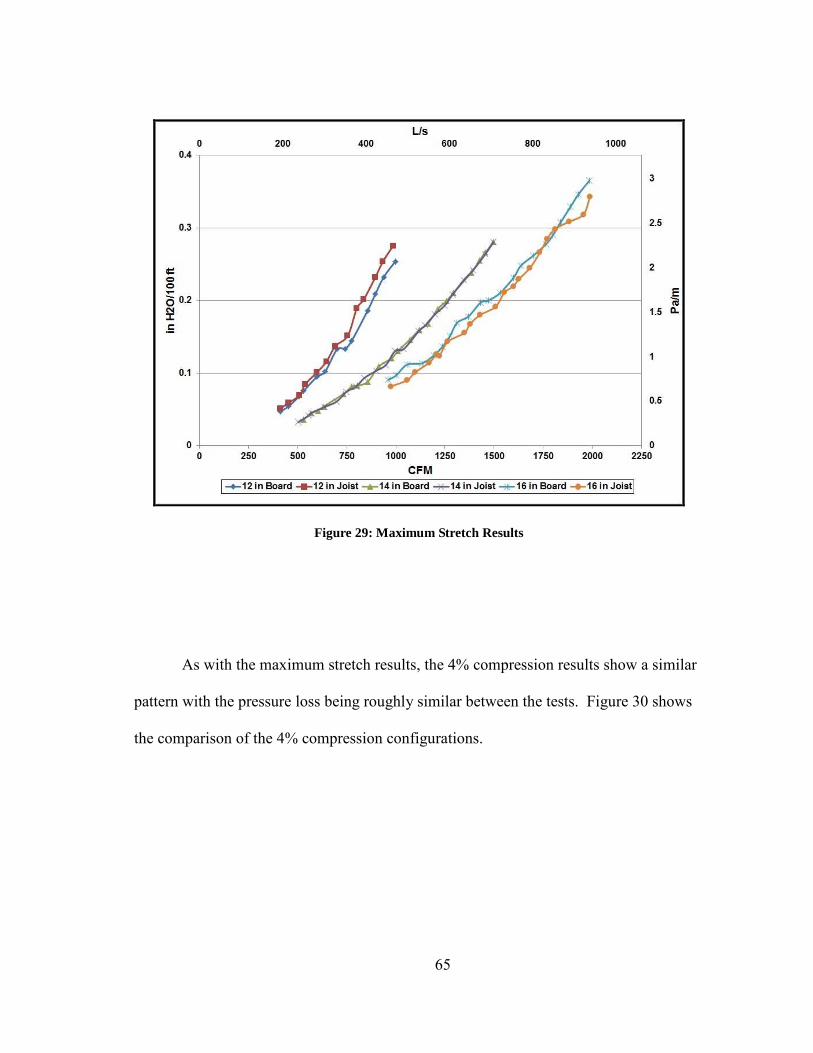
For this comparison, the results of the maximum stretch flexible duct tests are

shown for each duct size. It can be seen that the pressure drop for each flow range is

similar between the three duct sizes. The difference comes from the flow ranges. As the

duct size increases, the flow rate range increases to maintain the same pressure drop.

Figure 29 shows the comparison of the maximum stretch configurations for each duct

size.

65

Figure 29: Maximum Stretch Results

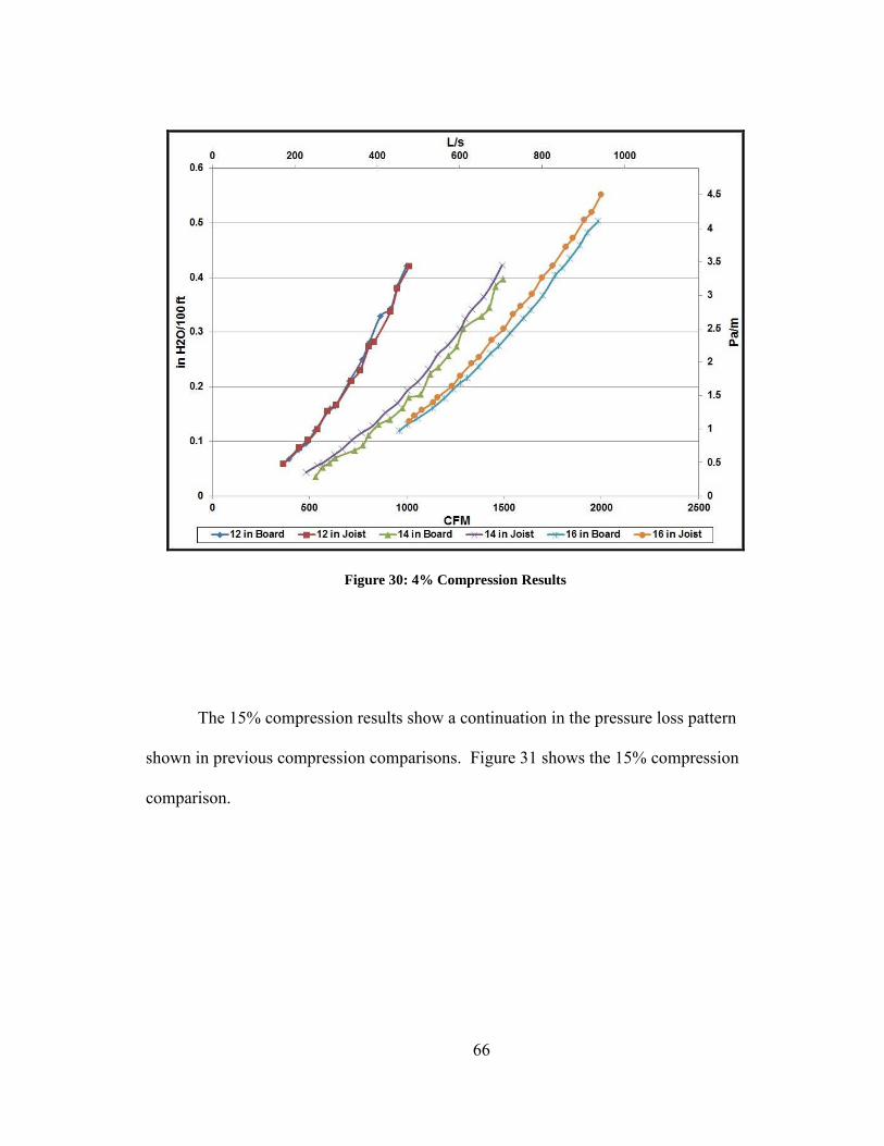
As with the maximum stretch results, the 4% compression results show a similar

pattern with the pressure loss being roughly similar between the tests. Figure 30 shows

the comparison of the 4% compression configurations.

66

Figure 30: 4% Compression Results

The 15% compression results show a continuation in the pressure loss pattern

shown in previous compression comparisons. Figure 31 shows the 15% compression

comparison.

67

Figure 31: 15% Compression Results

The pressure loss pattern continues to be seen in the 30% compression

comparisons. Figure 32 shows the 30% compression comparison.

68

Figure 32: 30% Compression Results

For the final compression comparison, the pressure loss pattern continues to be

present and is consistent with the previous compression comparisons. Figure 33 shows

the 45% compression comparison.

69

Figure 33: 45% Compression Results

70

CHAPTER X

ERROR ANALYSIS

Potential errors in this study arise from multiple sources including sensor

inaccuracies, excessive air leakage in system, compression irregularities, random error

and various other sources. Multiple measures were undertaken during the design, setup

and data collection phases in an effort to minimize errors in the study.

For sensor accuracy error minimization, all sensors selected to be used in the test

setup had an accuracy of no greater than 2% of full scale. Relevant specifications for all

the sensors utilized in this study can be found in Table 1. All sensors came with NIST-

traceable calibration certificates. An analysis of the sensor accuracies was performed to

review their contribution to the errors in the data.

The following inputs were utilized in the analysis:

∆Pnoz Measured pressure differential across nozzle board (in H2O) (Pa)

Sensor accuracy – 0.5% FS

Sensor error - ±.0025 in H2O

Tdb Dry bulb temperature determined by average of T1 and T2. (°F) (°C)

Sensor accuracy – 0.3% FS

Sensor error - ±0.6°F

Pb Barometric pressure collected from weather data from Easterwood

Airport (in-Hg) (kPa)

Sensor accuracy – unknown

Assumed sensor error – 1 in-Hg

71

Twb Wet bulb temperature determined using pyschrometric properties of air

using dry bulb temperature and relative humidity (°F) (°C)

Sensor accuracy – Based upon error of humidity sensor – 2% FS

Sensor error - ±1.6°F

Tamb Ambient temperature of testing area at time of test. (°F) (°C)

Sensor accuracy - 0.3% FS

Sensor error - ±0.6°F

Pnoz1 Static pressure prior to nozzle board. (in H2O) (Pa)

Sensor accuracy – 0.5% FS

Sensor error - ±.0025 in H2O

Applying these sensor errors to the input values in the Flow Calculator

Spreadsheet presented in Chapter 4, minimum and maximum CFM error is found. These

CFM values are then inputted into the curve-fit approximation equations to find

maximum and minimum pressure drop per 100 ft. The differences between the

maximum pressure drop and the measured press drop and the minimum pressure drop

and the measured pressure drop are found. These values are then divided by the

measured pressure drop to find the estimated error. For all of the data collected over all

compressions and duct sizes, the maximum calculated error was never greater than

±3.8%. The largest observed pressure loss in any of the tested configurations was 1.47

in H2O/100 ft. which corresponds to a calculated error of 0.056 in H2O/100 ft.

72

Error potential from excessive air leakage was minimized by performing total system air

leakage tests prior to data collection. This process was previously detailed in Chapter 7

– Test Methodology.

To minimize the potential impact of random error during the data collection

phase, the DAQ board registers values for each sensor based upon the individual

sensor’s response time as shown in Table 3. For each flow rate, the DAQ board reports

values every second for a total of 50 seconds. The average of these 50 values provides

the data points used in the data analysis.

It is believed that the majority of the error in this study fell into the category of

compression irregularities. As discussed earlier, the amount of compression in the

ductwork was based upon the length of duct at a maximum stretch position. For a 30

foot maximum stretch piece of flexible duct, the length of the flexible duct after 45%

compression was 16.5 feet. Approximate uniformity of the flexible duct’s vapor barrier

along the length of the compressed ductwork was observed during the setup.

Unfortunately, there was not a way to verify the uniformity of the single-helix duct liner.

This uncertainty in the uniformity of the interior duct liner leads to variations in

repeatability and the potential for error in the testing.

73

CHAPTER XI

COMPARISON WITH PREVIOUS WORK

Lawrence Berkeley National Laboratory (LBNL) Research

Research performed at Lawrence Berkeley National Laboratory (LBNL)

examined the effects of compression on the static pressure loss in flexible duct

(Abushakra et al., 2004)3. This research utilized a draw-through configuration to test

compression ratios of maximum stretch, 15% and 30%. This research tested these

compression ratios for 6”, 8” and 10” duct diameters. Due to the tested duct sizes and

the draw-through configuration, the data from LBNL and this study cannot be directly

compared. Review of the results for the three compression ratios tested at LBNL provide

evidence for increased pressure loss with increasing compression ratio, which was

consistent with the results of this study.

Texas A&M University Research

Research performed at Texas A&M University also examined the effects of

compression on static pressure loss in flexible duct (Weaver and Culp, 2007)25. Two

main differences in this research as compared to the LBNL research are the use of a

blow-through configuration in place of a draw-through configuration and the addition of

two compression ratios (4% and 45%). The setup and compression ratios in this

previous Texas A&M research is similar to the setup and compression ratios of this

study. Because this previous research also utilized the three smaller duct diameters,

direct comparison of results could not be performed. As with the LBNL research, review

74

of the data from the Texas A&M research also shows increased pressure loss at increased

compression ratios.

Trane Ductulator (Trane Co. 1976)20

The data from this study was also compared to the values included in a Trane

ductulator, which is commonly used in industry. The ductulator uses inputs of flow rate

and duct size to calculate estimated static pressure loss. Compression of ductwork was

not a variable in the most ductulators. Based upon the data from this study and the study

by Kevin Weaver, recent ductulators have incorporated some flexible duct compression

as a variable. Excessive errors are possible when using this method for flexible duct

design due to its inability to account for the duct compression ratio. Table 4 compares

the ductulator values with data from this study at representative flow rates along with an

error factor. Error between the ductulator values and the measured values is determined

using the following equation:

Ductulator

Measured

P

PError

∆∆= (11.1)

75

Table 3: Ductulator Comparison

Flow Maximum

Stretch 4%

Compression 15%

Compression 30%

Compression 45%

Compression

CFM in H2O in H2O in H2O in H2O in H2O

Ductulator

12" 500 0.055

14" 800 0.064

16" 1200 0.070

Measured

12" 500 0.068 0.106 0.139 0.216 0.320

14" 800 0.083 0.117 0.194 0.280 0.409

16" 1200 0.133 0.178 0.279 0.408 0.402

Error

12" 500 1.236 1.927 0.527 3.927 5.818

14" 800 1.297 1.828 3.031 4.375 6.391

16" 1200 1.900 2.543 3.986 5.829 5.743

76

CHAPTER XII

DEVELOPMENT OF PRESSURE DROP CORRECTION FACTORS

The currently accepted method to determine the pressure loss through flexible

duct includes estimating the compression amount and applying a correction factor for the

flexible duct. This method can be found in the ASHRAE Handbook of Fundamentals

(ASHRAE, 2009)7. The results of this research are intended to provide additional

information to be incorporated into this current methodology.

Research performed at LBNL (Abushakra et al., 2004)3 developed correction

factors for 6”, 8” and 10” duct diameters for compression ratios of maximum stretch,

15% and 30%. This research will add correction factors for 12”, 14” and 16” duct for

the five compression ratios tested.

The first step in the development of pressure drop correction factors (PDCF) for

this study was to develop power-law models for each compression ratio for each duct

size. This was done by plotting the pressure loss per 100 ft. values versus their

corresponding flow rate. Once all values of pressure loss versus flow rate at plotted for a

given compression ratio, a power equation trend line is mapped onto the plotted data.

This trend line’s equation represents the power-line model for the given compression and

duct size. The power-line model can be utilized to estimate the pressure loss per 100 ft.

for a given flow rate and is characterized by the following general equation:

nFlowCP *= (12.1)

77

The equation contains a coefficient of C, the flow rate in CFM, and an exponent, n. The

value of the exponent (n) is typically assumed to be two. In actual applications, this

value fluctuates around the value of two.

Once these equations are determined, they can be used to develop the PDCF.

The PDCF is a multiplier which can be used to estimate the static pressure loss in

flexible duct under compression. The PDCF is calculated, for a given flow rate, as the

ratio of the compressed pressure loss to the maximum stretched pressure loss:

MSP

PPDCF

∆∆= (12.2)

where ∆P is the pressure loss at a particular compression and ∆PMS is the pressure loss at

a maximum stretched position. For this study, a representative flow rate was chosen for

each duct size to develop the PDCFs for each compression ratio. For 12” duct, the

PDCFs were developed based upon a flow rate of 400 cfm. For 14” duct, the PDCFs

were developed based upon a flow rate of 600 cfm. For 16” duct, the PDCFs were

developed based upon a flow rate of 1000 cfm. Figure 34 shows the PDCFs developed

in this study. These PDCFs were incorporated into the existing PDCFs in the ASHRAE

Handbook of Fundamentals (ASHRAE, 2009)7.

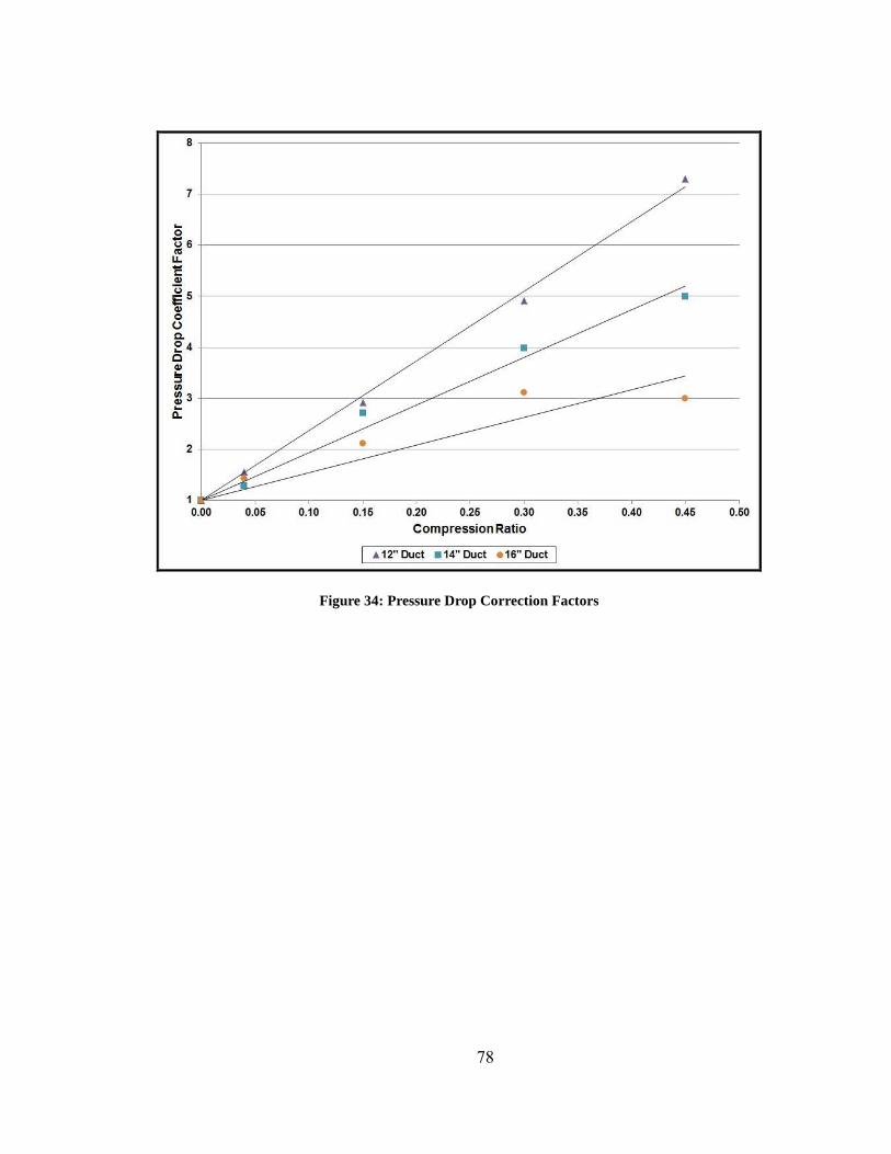
78

Figure 34: Pressure Drop Correction Factors

79

CHAPTER XIII

DISCUSSION

The results from this study demonstrate the importance of proper installation of

non-metallic flexible duct in actual applications. The compression of flexible duct has

the potential to increase the duct static pressure loss by as much as five times that of

fully stretched duct. This demonstrates that proper installation of duct systems becomes

just as important as duct system design.

A factor that was found to affect the amount of pressure drop was the geometric

configuration of the duct. Industry standards call for the duct to be installed straight.

Any amount of change in the duct from being completely straight will increase the

pressure loss through the duct. A straight duct introduces the air flow to the minimal

amount of surface area. Any change in that path of air flow results in exposure to greater

interior surface areas. The compression amount changes the effective diameter of the

duct. With an increase in compression ratio comes a decrease in the diameter that the air

flow encounters. This decrease in diameter directly increases the static pressure loss.

This effect is less noticeable in larger duct diameters as compared to smaller duct

diameters.

The compression of the flexible duct creates small pockets in the geometry of the

inner duct between the metal wire helix. The air flow into these pockets can create

vortices within the air stream which causes greater turbulence in the air flow. This

increase in turbulence within the air stream results in increased pressure loss in the duct.

80

CHAPTER XIV

CONCLUSIONS

This research collected static pressure loss values for various compression

configurations for 12”, 14”, and 16” non-metallic flexible duct. Conclusions gathered

from this research are as follows:

1. Installation of non-metallic flexible duct in straight run configurations

should be as close to a fully stretched manner as possible. If the flexible duct

cannot be installed fully stretched, it should have no greater than 4%

compression as set forth in the installation instructions by the ADC (ADC 2003)5.

2. For duct compression greater than 4%, flexible duct can have pressure

drops four to ten times the pressure drop in rigid sheet metal ducts.

3. Flexible duct installed at compressions greater than 4% demonstrate

potential for decreased airflow and system performance in commercial HVAC

systems.

4. Any time flexible duct is utilized in a HVAC system, the duct should be

properly sealed using the methods specified by the ADC. Proper sealing of the

ductwork will reduce the amount of air leakage in the system which will in turn

lower the supply fan usage in the HVAC system.

81

REFERENCES

1. Abushakra, B., D. Dickerhoff, I. Walker and M. Sherman. 2001. Laboratory

Study of Pressure Losses in Residential Air Distribution Systems. Lawrence

Berkeley National Laboratory Report LBNL-49293, Berkeley, CA.

2. Abushakra, B., D. Dickerhoff, I. Walker and M. Sherman. 2002. A Study of

Pressure Losses in Residential Air Distribution Systems. Proceedings of the ACEEE

Summer Study 2002, American Council for an Energy Efficient Economy,

Washington, D.C., Lawrence Berkeley National Laboratory Report LBNL-49700,

Berkeley, CA.

3. Abushakra, B., I. S. Walker, M. H. Sherman. 2004. Compression Effects on

Pressure Loss in Flexible HVAC Ducts. International Journal of Heating,

Ventilating, Air-Conditioning and Refrigeration Research, V. 10 (3), pp. 275-289.

4. ACCA. 2009. Residential Duct Systems. Manual D. Air Conditioning

Contractors of America, Washington, DC.

5. ADC. 2003. Flexible Duct Performance and Installation Standards, 4th Edition.

Air Diffusion Council, Shaumburg, IL.

6. Altshul, A.D. and P.G. Kiselev. 1975. Hydraulics and Aerodynamics. Stroisdat

Publishing House, Moscow, USSR.

7. ASHRAE. 2009. ASHRAE Handbook of Fundamentals. American Society of

Heating, Refrigerating and Air-Conditioning Engineers, Atlanta, GA.

82

8. ASHRAE. 1999. ASHRAE Standard 120, Methods of Testing to Determine Flow

Resistance of HVAC Air Ducts and Fittings, June 1999. American Society of

Heating, Refrigerating and Air-conditioning Engineers, Atlanta, Georgia.

9. ASHRAE. 1986. ASHRAE Standard 42.1, Standard Method for Temperature

Measurement, June 1986. American Society of Heating, Refrigerating and Air-

Conditioning Engineers, Atlanta, GA.

10. ASHRAE. 1987. ASHRAE Standard 42.2, Standard Methods for Laboratory

Airflow Measurement, June 1987. American Society of Heating, Refrigerating and

Air-Conditioning Engineers, Atlanta, GA.

11. ASHRAE. 1989. ASHRAE Standard 42.3, Standard Method for Pressure

Measurement, January 1989. American Society of Heating, Refrigerating and Air-

Conditioning Engineers, Atlanta, GA.

12. Bricker, E.J. 1961. Field Checking and Testing of Ventilation and Air

Conditioning Systems, ASHRAE Journal, May, pp. 10-72

13. Fellows, J.R. 1939. Power Savings through Static Pressure Regain in Air Ducts,

HPAC, V.11 (4) pp. 219-222

14. Graham, J.B. 1996. Duct System Pressure Gradient Diagrams and the Beer

Cooler Problem, Heating, Piping and Air Conditioning, August, pp. 63-66, 80.

15. Harrison, E. 1965. Balancing Air Flow in Ventilating Duct Systems, IHVE

Journal, V. 33, pp. 201-226

83

16. Kokayko, M., J. Jolton, T. Beggs, S. Walthour, and B. Dickson. 1996. Residential

Ductwork and Plenum Box Bench Tests. IBACOS Burt Hill Project 95006.-13.

Pittsburgh, PA

17. Moody, L.F. 1944. Friction Factor for Pipe Flow. ASME Transactions, Vol. 66,

pp. 671-678.

18. Scott K.B., 1986. Don't Ignore Duct Design for Optimized HVAC Systems,

Specifying Engineer, No. 62, January, 1986.

19. Shieh Chun-Lun. 1983. Simplified Static-Regain Duct Design Procedure,

ASHRAE Transactions. V.89 (2a), pp. 78-94.

20. Trane Company. 1976. Explanation of the Trane Air Conditioning Ductulator.

Product Explanation. Trane Co, Carrollton, TX.

21. Tsal, R.J. and H.F. Behls, 1986. Evaluation of Duct Design Methods. ASHRAE

Transactions, Vol. 92 (1A), pp. 347-361.

22. Tsal, R.J. and H.F. Behls. 1988a. Fallacy of the Static Regain Duct Design

Method, ASHRAE Technical Data Bulletin, ASHRAE, Atlanta, GA

23. Tsal, R.J., H.F. Behls, and R. Mangel 1988b. T-Method Duct Design Part I:

Optimization Theory ASHRAE Transactions, V. 92, Part 1A

24. Tsal, R.J. 1989. Altshul-Tsal Friction Factor Equation. Heating, Piping and Air

Conditioning, July, 1989.

25. Weaver, K., and C. Culp. 2007. Static Pressure Loss in Nonmetallic Flexible

Duct, ASHRAE Transactions, V. 113, Part 2.

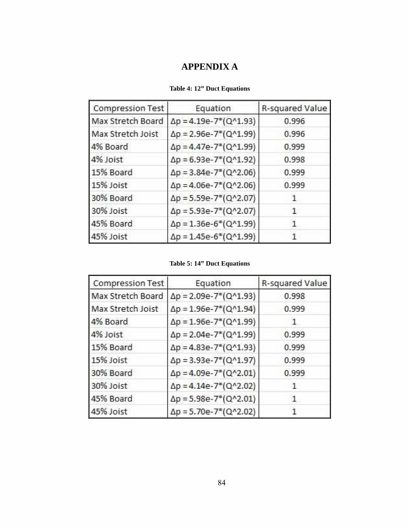
84

APPENDIX A

Table 4: 12” Duct Equations

Table 5: 14” Duct Equations

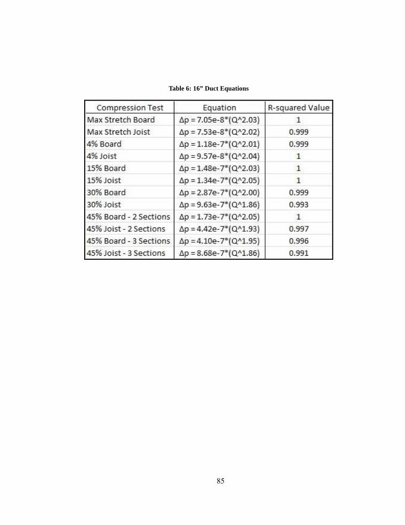
85

Table 6: 16” Duct Equations