static and dynamic moments for any plane within a straight

1

Static and Dynamic Moments for any Plane within a Straight Solid Slab Bridge Caused

by the Crossing of a Truck

Omar Mohammed 1,3 *, Arturo González 2,3

1 Researcher, email: [email protected]

2 Associate Professor, email: [email protected]

3 School of Civil Engineering, University College Dublin, Ireland

* Corresponding author. Postal address: School of Civil Engineering, University College Dublin,

Newstead, Belfield, Dublin 4, Ireland.

Phone number: +353 1 7163229.

Email address: [email protected], [email protected]

Abstract

A lot of research has been carried out to explain the manner in which longitudinal moments of

a bridge respond to traffic. The total longitudinal bending moment is made of ‘static’ and

‘dynamic’ components, which vary with time as a result of the inertial forces of the bridge and

changes in value and point of application of the forces of the vehicle. However, there is limited

evidence about how bending moments at planes other than longitudinal, or twisting moments,

act in response to a moving vehicle. For the first time in the literature, this paper analyses the

total resultant moments (‘static’ + ‘dynamic’) for any plane orientation (from 0 to 360°) at any

location of a solid slab deck due to the crossing of a vehicle. The bridge is modelled as a simply

supported straight orthotropic plate and the vehicle is modelled as a three-dimensional 5-axle

articulated system composed of interconnected sprung and unsprung masses. Simulations are

performed for three vehicle transverse paths and three speeds. Using Wood and Armer

equations, the resultant moment at any plane orientation can be obtained from equilibrium of

bending and twisting moments acting on longitudinal and transverse planes. Maximum twisting

mailto:[email protected]

2

moments develop in planes at 45° with longitudinal and transverse planes. Bending moments

reach maximum and minimum values at longitudinal and transverse planes. Nevertheless, the

moments acting on other plane orientations cannot be ignored in order to accurately assess

whether the moment capacity of the bridge provides adequate safety. Therefore, the amount of

slab reinforcement will be sufficient provided that the moment capacity exceeds the applied

moment for any location and plane. Critical locations with highest values of sagging, hogging

and twisting are identified in the bridge, and the dynamic amplification associated to the

applied moments is evaluated. Bridge codes such as the Eurocode employ a unique built-in

dynamic amplification factor for moment that depends only on the bridge length and the

number of lanes. This paper shows how to perform an improved assessment allowing for

changes in dynamic behaviour with location and plane orientation, which may prevent needless

expense in bridge rehabilitation.

Key words: Vehicle Bridge Interaction; Bridge slab; Dynamic Amplification Factor;

Moments; Traffic loading; Bridge dynamics

1. Introduction:

Solid slab deck sections are commonly found in short span bridges, spanning to about 21 m

[1,2]. These are made of in-situ or a mix of precast inverted T-beams and in-situ concrete [3].

For medium-span bridges, there is a substantial increase in the self-weight of the solid slab and

the challenges of construction; hence, beam-and-slab decks are generally preferred. The

thickness of the solid slab deck is significantly smaller than the width and length. Solid slab

decks carry out vertical loads to the supports by a combination of moments and shear forces.

Thin plate theory is commonly accepted for modelling the bending behaviour of these decks.

The deck is assumed to be uncompressible and the deflection of the plate is attributed to

3

bending alone (i.e., shear distortion makes no substantial contribution to deflection). These

assumptions are a simplification of the true behaviour, but are justified by the fact that the

performance of these bridge slabs, being relatively thin, is dominated by bending rather than

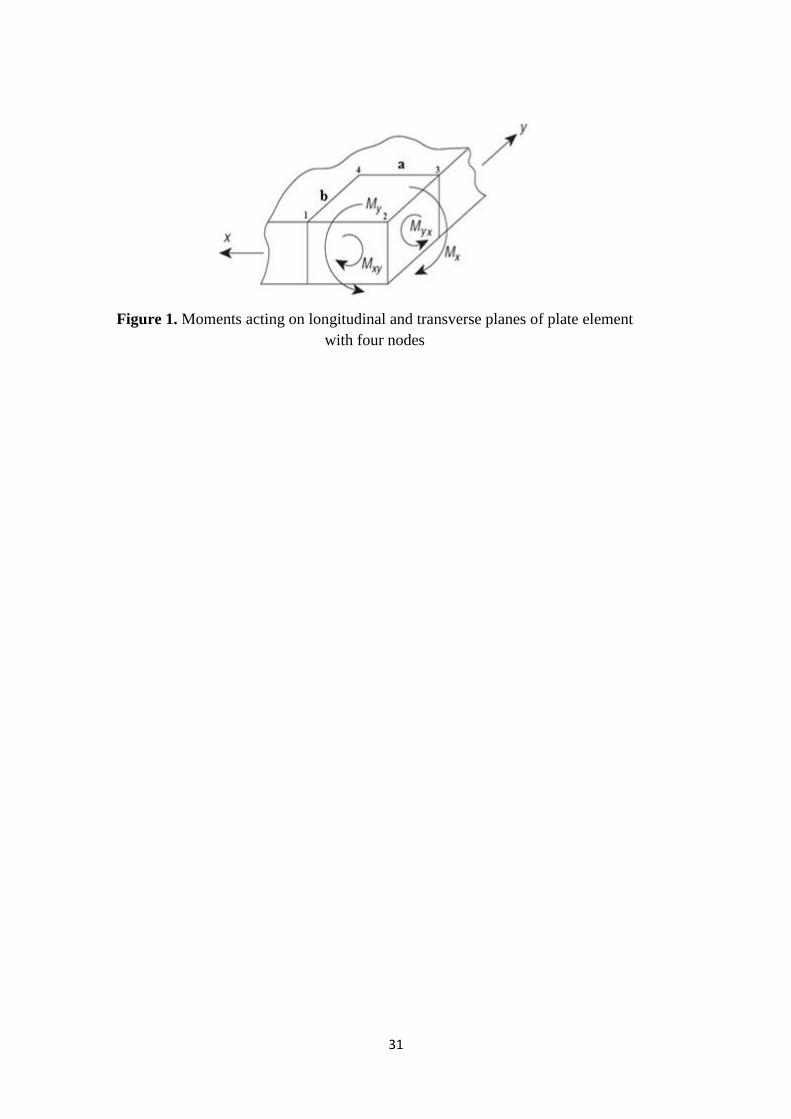
shear deformation [5]. Figure 1 shows the total moments acting about mid-depth of a plate

element with longitudinal dimension ‘a’ and transverse dimension ‘b’.

The bending capacity of the slab must be sufficient to withstand not only the maximum bending

moments at longitudinal and transverse planes, but any moment regardless of the plane. For

that purpose, the total moments, Mx and My, acting in longitudinal and transverse planes

respectively, can be considered as vectors and combined to attain the resultant moment for a

plane at any specific angle from imposing equilibrium. Here, it is worth to mention the role

played by Wood and Armer in slab design, who suggest an expression to determine the bending

moment capacity per unit breadth in longitudinal and transverse directions (orthogonal

reinforcement) necessary to withstand the maximum applied bending moment irrespective of

plane orientation [4]. The notation mx (= Mx / b) refers to bending moment per unit breadth

acting on a plane of normal the longitudinal direction x (i.e., perpendicular to the boundary

delimited by the bridge supports). Similarly, the transverse bending and twisting moments per

unit breadth are represented by the symbols my (= My / a) and mxy (= Mxy / b) respectively.

Therefore, mxy is equal to myx due to equilibrium. There are numerical and experimental

investigations on how these perpendicular moments affect the static response of a concrete slab

[5-9]. Longitudinal stresses 𝜎𝑥 due to mx, are found to be larger than transverse stresses 𝜎𝑦, due

to my, with first cracks developing at 45°. As the span of the slab gets longer, it is evident that

the static longitudinal bending becomes more dominant. In the case of a concrete slab bridge

traversed by a vehicle, there will be a ‘dynamic’ component in addition to the ‘static’

component [10]. Bakht and Pinjarkar [11], Inbanathan and Wieland [12] and Wang and Deng

[13] quantify this ‘dynamic’ component with a term named dynamic Impact Factor (IM), which

4

takes into account the maximum of the two responses (‘dynamic’ and ‘static’). Dynamic Load

Allowance (DLA) [14–16] and Dynamic Amplification Factor (DAF) [17–19] are other

popular definitions to characterize the ‘dynamic’ component. DAF is defined as the ratio of

maximum total (‘static’ plus ‘dynamic’ components) response to the maximum ‘static’

response at a specific bridge location. Cantero et al. [20] put forward a new definition, i.e., Full

Dynamic Amplification Factor (FDAF), to cover for the fact that the selected bridge location

may not hold the worst possible scenario. FDAF is given by the ratio of the maximum total

response taking into account all bridge sections to the maximum ‘static’ response at a particular

section taken as reference (typically mid-span). By definition, FDAF is always equal or greater

than DAF for a given section. A considerable amount of information is provided by earlier

authors on DAF or equivalent terms due to a moving load. However, most of existing literature

investigate deflections or the longitudinal bending moment/strains (i.e., mx), and only a few

publications have examined DAF associated to other load effects (i.e., DAF of shear by [21]).

Therefore, there is a need in the literature to address the dynamic impact experienced by

moments in planes other than longitudinal as a result of the moving traffic. Without this

information, it is not possible to gather an accurate picture of the true moment capacity needed

to ensure the safety of a slab. For this purpose, Section 2 describes the mathematical models

that will be employed to calculate the response of the bridge to a moving vehicle. The slab deck

is modelled using thin plate Finite Element (FE) theory and the truck is represented by a 5-axle

tractor and semitrailer configuration. Section 3 calculates bending and twisting moments acting

on longitudinal and transverse planes for a 9m long bridge, three transverse vehicle paths

(travelling centred over the bridge centreline and at other two eccentricities) and three vehicle

speeds (15, 20 and 25 m/s). Section 4 calculates moments (‘static’ and total) for any plane

orientation , where is the angle that the normal to the plane makes with the x-direction (i.e.,

= 0 is the longitudinal plane where mx is acting, and = 90 is the transverse plane where my

5

is acting). Finally, the critical locations holding the largest moments are discussed and Section

6 provides conclusions.

2. Simulations Models

2.1. Bridge Model

A simply supported solid slab deck of 9 m width and 9 m span length is considered. The bridge

is modelled as an orthotropic thin plate discretized using the FE method into a mesh made of

0.5 m × 0.5 m plate elements. The standard Kirchoff plate element [22,23] contains four nodes

and three Degrees Of Freedom (DOFs) per node: the vertical displacement and the rotations

about the x and y axes. This discretization of the displacement field results in a third-order

polynomial containing 12 terms. Zienkiewicz [22] and Reddy [23] explain in detail why such

a discretization can lead to a discontinuity of the slope across inter-element boundaries. One

solution to the problem of the non-conforming plate element is to impose continuity conditions

as an additional DOF, such that the fourth DOF at each node is the second derivative of w with

respect to x and y. This fourth DOF is also known as nodal twist. Bogner et al [24] first proposed

this method for isotropic plates, where the interpolation functions for the DOFs were defined

as the products of the Hermite shape functions for an Euler-Bernoulli beam. The full derivation

of the 16 DOF orthotropic C1 plate element employed in this paper can be found in Rowley

[25]. Vertical displacements are prevented at each node of end sections above supports. In total,

the bridge has 1444 DOFs. The properties of the bridge are presented in Table 1 based on

[26,27].

6

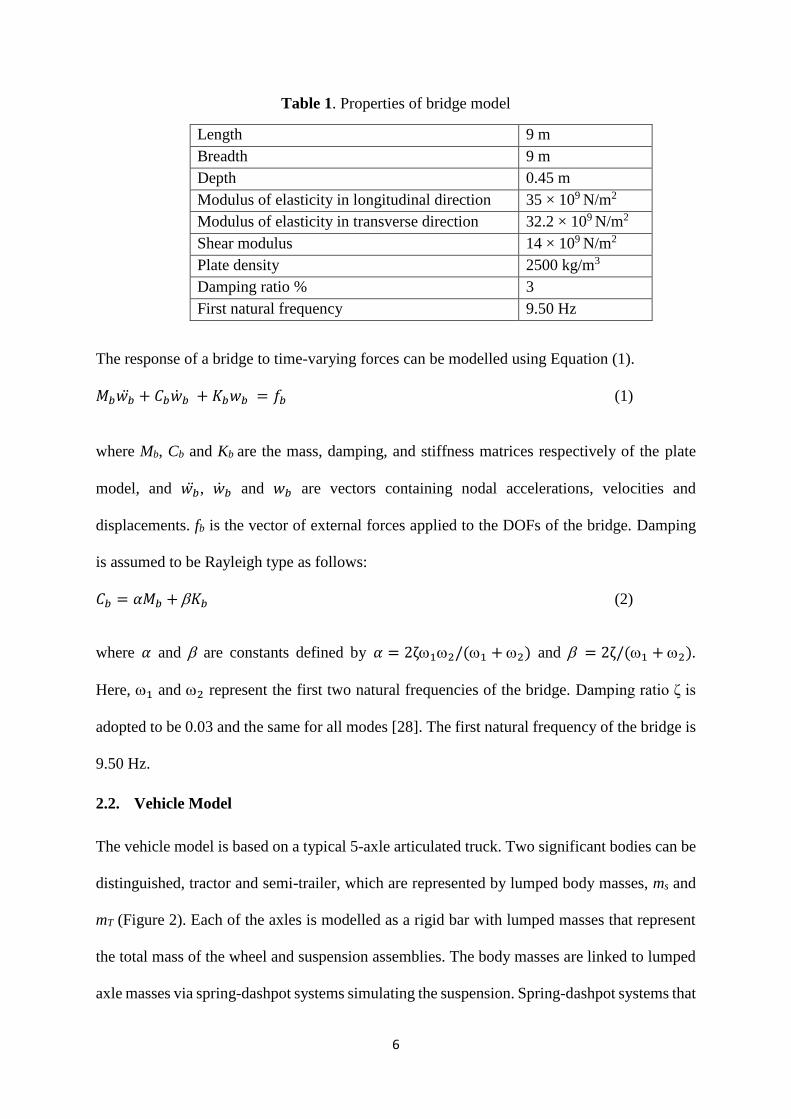
Table 1. Properties of bridge model

Length 9 m

Breadth 9 m

Depth 0.45 m

Modulus of elasticity in longitudinal direction 35 × 109 N/m2

Modulus of elasticity in transverse direction 32.2 × 109 N/m2

Shear modulus 14 × 109 N/m2

Plate density 2500 kg/m3

Damping ratio % 3

First natural frequency 9.50 Hz

The response of a bridge to time-varying forces can be modelled using Equation (1).

𝑀𝑏𝑤�̈� + 𝐶𝑏�̇�𝑏 + 𝐾𝑏𝑤𝑏 = 𝑓𝑏 (1)

where Mb, Cb and Kb are the mass, damping, and stiffness matrices respectively of the plate

model, and 𝑤�̈�, �̇�𝑏 and 𝑤𝑏 are vectors containing nodal accelerations, velocities and

displacements. fb is the vector of external forces applied to the DOFs of the bridge. Damping

is assumed to be Rayleigh type as follows:

𝐶𝑏 = 𝛼𝑀𝑏 + 𝐾𝑏 (2)

where 𝛼 and are constants defined by 𝛼 = 2ζ12/(1 + 2) and = 2ζ/(1 + 2).

Here, 1 and 2 represent the first two natural frequencies of the bridge. Damping ratio ζ is

adopted to be 0.03 and the same for all modes [28]. The first natural frequency of the bridge is

9.50 Hz.

2.2. Vehicle Model

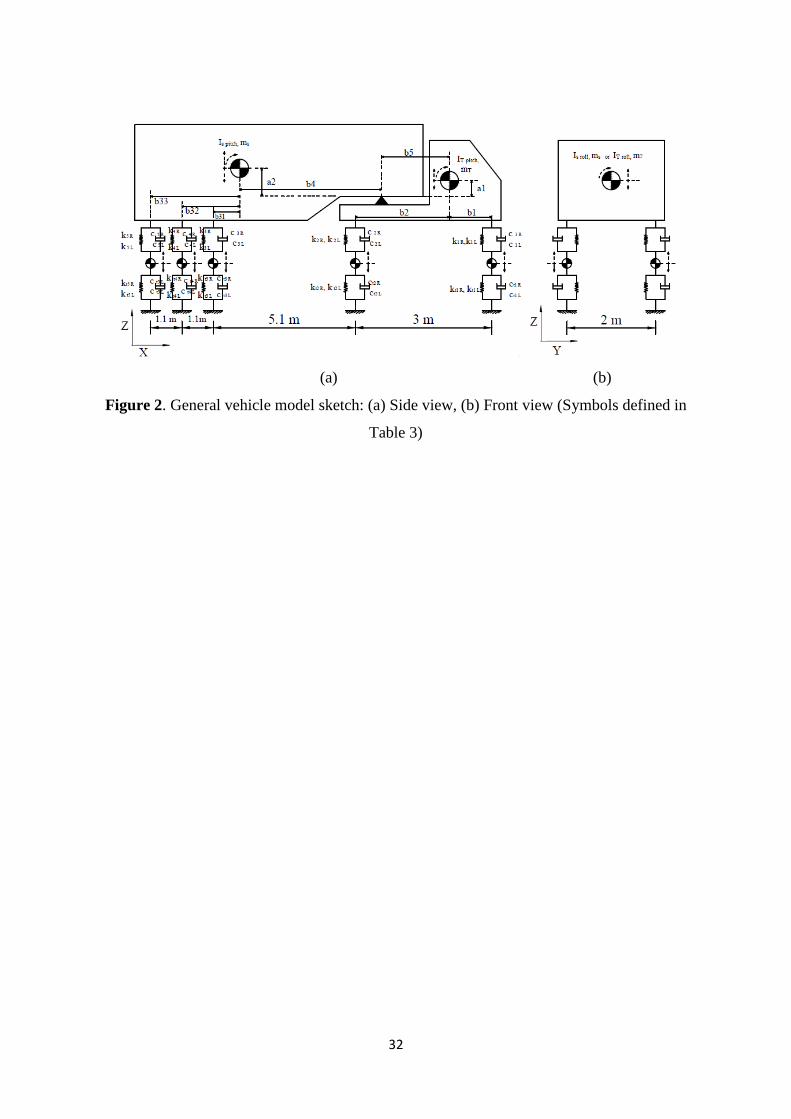
The vehicle model is based on a typical 5-axle articulated truck. Two significant bodies can be

distinguished, tractor and semi-trailer, which are represented by lumped body masses, ms and

mT (Figure 2). Each of the axles is modelled as a rigid bar with lumped masses that represent

the total mass of the wheel and suspension assemblies. The body masses are linked to lumped

axle masses via spring-dashpot systems simulating the suspension. Spring-dashpot systems that

7

resemble the tyres are used to connect the axle masses to the road surface. In total, the model

has 15 DOFs. Tables 2 and 3 provide the geometry and the mechanical properties of the vehicle

respectively, based on the work by [20,29].

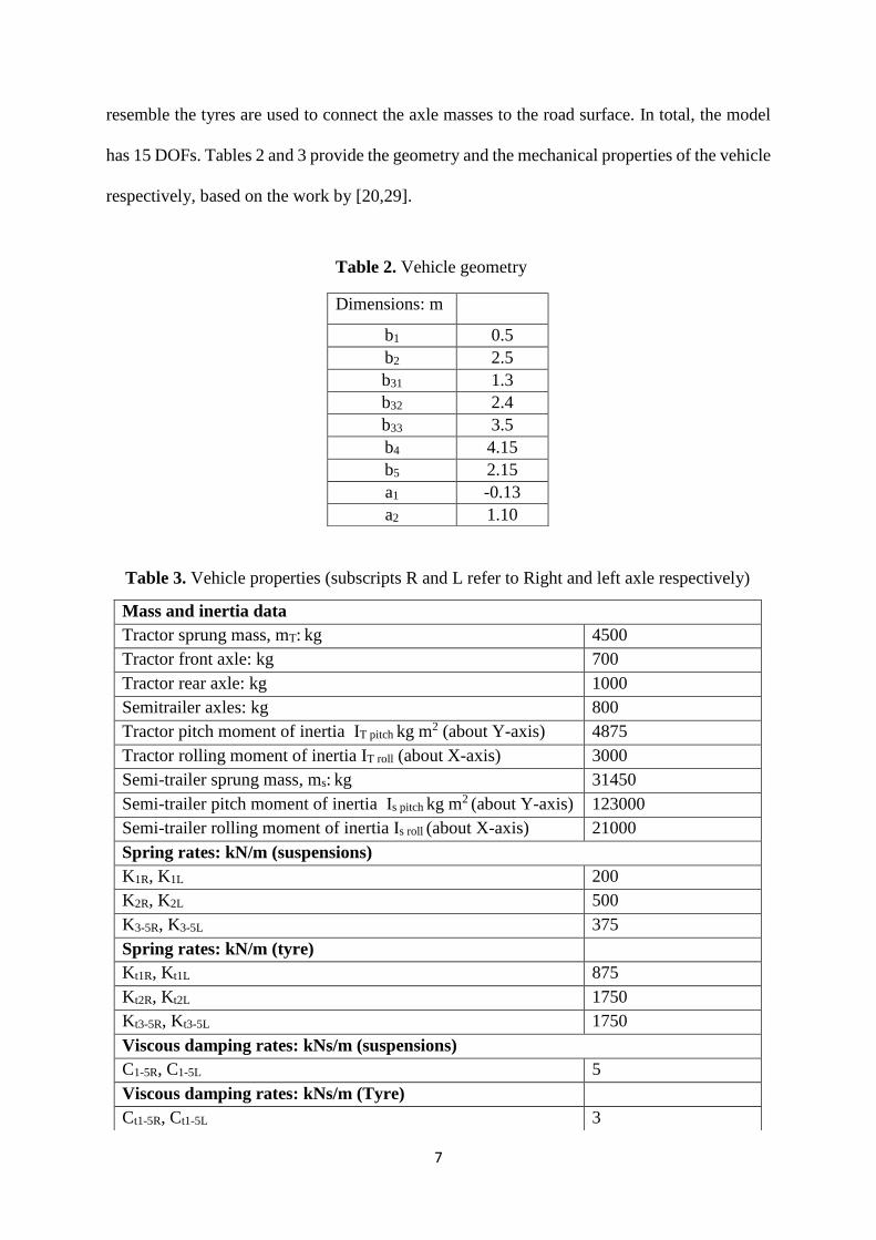
Table 2. Vehicle geometry

Dimensions: m

b1 0.5

b2 2.5

b31 1.3

b32 2.4

b33 3.5

b4 4.15

b5 2.15

a1 -0.13

a2 1.10

Table 3. Vehicle properties (subscripts R and L refer to Right and left axle respectively)

Mass and inertia data

Tractor sprung mass, mT: kg 4500

Tractor front axle: kg 700

Tractor rear axle: kg 1000

Semitrailer axles: kg 800

Tractor pitch moment of inertia IT pitch kg m2 (about Y-axis) 4875

Tractor rolling moment of inertia IT roll (about X-axis) 3000

Semi-trailer sprung mass, ms: kg 31450

Semi-trailer pitch moment of inertia Is pitch kg m2 (about Y-axis) 123000

Semi-trailer rolling moment of inertia Is roll (about X-axis) 21000

Spring rates: kN/m (suspensions)

K1R, K1L 200

K2R, K2L 500

K3-5R, K3-5L 375

Spring rates: kN/m (tyre)

Kt1R, Kt1L 875

Kt2R, Kt2L 1750

Kt3-5R, Kt3-5L 1750

Viscous damping rates: kNs/m (suspensions)

C1-5R, C1-5L 5

Viscous damping rates: kNs/m (Tyre)

Ct1-5R, Ct1-5L 3

8

The range of pitching and rolling body frequencies falls within 1.5 Hz to 4.5 Hz and the

hopping axle frequencies go from 9 Hz to 16 Hz (Table 4), in agreement with values published

by [30].

The static gross vehicle weight is distributed amongst axles 1 to 5 based on the percentages

given by [31]: 12.70 % (front axle), 27.70 % (2nd axle) and 19.87 % (any of the axles in the

rear tridem). Static wheel weights are given in Table 5.

Table 5. Static wheel weights (kN) (subscripts

R and L refer to right and left axle respectively) P1R, P1L 24.93

P2R, P2L 54.39

P3R, P3L 38.99

P4R, P4L 39.01

P5R, P5L 39.01

Table 4. 5-axle vehicle frequencies in Hz

symbol property value

fv1 Tractor bounce 1.48

fv2 Tractor pitch 2.3

fv3 Tractor roll 3.0

fv4 Semitrailer pitch 1.49

fv5 Semitrailer roll 1.58

fv6 1st axle hop left wheel 8.9

fv7 1st axle hop right wheel 8.9

fv8 2nd axle hop left wheel 10.7

fv9 2nd axle hop right wheel 10.7

fv10 3rd axle hop left wheel 11.6

fv11 3rd axle hop right wheel 11.6

fv12 4th axle hop left wheel 11.6

fv13 4th axle hop right wheel 11.6

fv14 5th axle hop left wheel 11.6

fv15 5th axle hop right wheel 11.6

9

The equations of motion of a vehicle model can be obtained imposing equilibrium of all forces

and moments that act on the masses. The terms in these equations can be ordered according to

the DOFs and placed in matrix form as follows:

𝑀𝑣𝑤�̈� + 𝐶𝑣�̇�𝑣 + 𝐾𝑣𝑤𝑣 = 𝑓𝑣 (3)

where Mv, Cv and Kv are mass, damping and stiffness matrices of the vehicle respectively, and

𝑤�̈�, �̇�𝑣 and 𝑤𝑣 are the vectors corresponding to nodal accelerations, nodal velocities and nodal

displacements. 𝑓𝑣 is a vector containing the time-varying forces imposed on the vehicle’s

DOFs. This model assumes negligible lateral and yaw movement.

2.3. Road Profile

The roughness of the road surface is a major cause of dynamic excitation in vehicle-induced

bridge vibrations [32–36]. An artificial road profile can be generated using the Power Spectral

Density (PSD) of vertical irregularities along with the inverse fast Fourier transform technique

explained by [37]. For each spatial wave frequency, a random phase angle ∅𝑖 is sampled from

a uniform probabilistic distribution in the range 0-2𝜋. An ‘A’ class road carpet, i.e. ‘very good’

according to the International Organization for Standardization (ISO 1995)[38], is produced

using a geometric spatial mean of 16 × 10−6 m3/cycle [39]. Finally, a moving average filter is

applied to the road irregularities across a distance of 0.24 m to simulate the tyre contact patch

[40,41]. Figure 3 shows the resulting class ‘A’ carpet used for the surface of the bridge. This

bridge surface is preceded by a 100 m approach generated using the same procedure. The

purpose of the road approach is to induce vibrations in the vehicle prior to entering the bridge

that will simulate initial conditions of dynamic equilibrium.

10

2.4. Uncoupled VBI Algorithm

An uncoupled Vehicle-Bridge Interaction (VBI) algorithm is employed for calculating the

response of the plate model to the crossing of the 5-axle truck at uniform speed. The equations

of motion of the vehicle (Equation (3)) and the bridge (Equation (1)) are treated as two separate

subsystems. These equations are solved via application of the Newmark-Beta direct integration

method with a time increment of 0.002 s and values for the integration constants of delta = 0.5

and beta = 0.25. An iterative process is carried out at each time step as follows. Initially, forces

acting on the DOFs of the vehicle (fv) are calculated using Equation (3) based on the road

profile ‘only’. The wheel forces defined by 𝑓𝑣 need to be converted to equivalent forces acting

on the bridge nodes (𝑓𝑏) before calculating the bridge response. Equation (4) is used to

distribute each wheel force from its point of application to the nodes of the plate element

directly underneath.

𝑓𝑏 = 𝐿 × 𝑓𝑣 (4)

where fb is a matrix p x 1, fv is a vector pf x 1, and L is an p × pf location matrix that relates the

pf wheel forces to equivalent forces acting on the p DOFs of the bridge. Each column of the

location matrix L maps one of the pf forces to the DOFs associated with the particular

underlying element as a product of the numerical value of the shape functions for that point in

time. In this way, the time-varying location matrix L becomes a function of the shape functions

of a 2D plate element as follows:

11

1 1 1

2 1 1 1 2 2

2 2 2 1

16 1 1 2 1 10 10

16 2 2 2 10 10

16

16 10 10

0 0 ... 0 ... 0

. . ... . ... .

( , ) . ... . ... .

( , ) ( , ) ... . ... .

. ( , ) ... ( , ) ... .

( , ) . ... ( , ) ... ( , )

. ( , ) ... . ... ( , )

. . ... ( , ) ... .

. . ... . ... ( , )

. .

i i

i i

i i

N x y

N x y N x y

N x y N x y

L N x y N x y N x y

N x y N x y

N x y

N x y

... . ... .

0 0 ... 0 0 0

(5)

where N1( xi ,yi) to N16( xi ,yi) are the shape functions corresponding to the 16 DOFs of the plate

element. Here, column i represents the distribution of the wheel force i to the DOFs of the

element that the force is acting on, and xi and yi are the time-varying longitudinal and transverse

distances from the wheel force i to a node of the element. I.e., columns 1, 2, 3 … and 10

distribute the first, second, third … and tenth wheel forces of the vehicle respectively to the

DOFs of the bridge. The four shape functions corresponding to the vertical displacement, the

rotations about the x- and y- directions and the twist of one node of the plate element are given

by Equations (6), (7), (8) and (9) respectively.

2

1 3 3

1( , ) ( 2 )( ) ( 2 )( )i i i i i iN x y b y b y a x x a

a b (6)

2 2

2 3 2

1( , ) ( ) ( 2 )( )i i i i i iN x y y b y a x x a

a b (7)

3 2 3 2 2 2 2 2

3

2 2 2 2 2 2 2 2 2 2 2

2 4

( , ) ( )( 2 2

114 10 2 18 12 )

i i i i i i i i i i

i i i i i i i i i i

N x y x b y x ab x b a b x y ab x y b

y a b x y ab x y b y a b x y a x y aa b

(8)

2 2 2 2 2

4

2 2 2 2

2 3

( , ) ( )( 2 7

15 9 6 )

i i i i i i i i

i i i i i i i

N x y x y b y x ab x b a b x y ab

x y b y a b x y a x y aa b

(9)

where a and b are the dimensions of the plate element.

12

The vector fb is then employed in Equation (1) to calculate bridge displacements (wb), which

are subsequently employed together with the road profile to recalculate the vehicle forces fv in

a 2nd iteration, and so on. The stopping criterion employed here is based on [42], who specify

that the variation between the bridge deflections, wb, of two consecutive iterations must be less

than 2% of the highest bridge deflection. Once the criterion is achieved, the forces of the vehicle

are positioned at new coordinates on the bridge and the iterative process is carried out again.

Cantero et al. [2, 29, 43] provide further details on this uncoupled algorithm. The latter is coded

with the help of MATLAB because of the flexibility it offers. The program has been validated

against alternative VBI approaches and experimental data [30]. The simulations are carried out

using a computer with 32 GB RAM memory, i7-3770 core processor and CPU @ 3.4 Hz

running MATLAB 2014 on a Windows 7 platform. The computational time to obtain the

responses at all FE nodes for one crossing of the vehicle is less than one minute.

Figure 4 depicts the three transverse positions that are considered for the path of the vehicle.

There is an equal distance between the centre of gravity of the vehicle’s body mass and the

outer and inner wheels (Figure 2(b)). The paths of this centre of gravity are at a distance of 0

m (path ‘2’), 1.5 m (path ‘1’) and 3 m (path ‘3’) from the bridge longitudinal centreline. If the

bridge had two traffic lanes situated symmetrically with respect to the bridge centreline, path

‘1’ would approximately correspond to the vehicle travelling in the middle of the lane, path ‘2’

to the vehicle travelling in the middle of the bridge, and path ‘3’ to a rare situation where the

vehicle is travelling partially on the shoulder. The distribution of moments in the slab are

calculated for nine vehicle scenarios covering these three transverse paths and three speeds:

15, 20 and 25 m/s.

13

3. Moments in Longitudinal and Transverse Planes

The total (‘static’ + ‘dynamic’) values of the FE DOFs are calculated using the procedure

described in Section 2.4. mx, my and mxy are then determined for each node of the bridge FE

based on the shape functions and constitutive equations of the plate element [22]. ‘Static’

displacements and rotations can be obtained using Equation (1) for every position of the truck,

assuming vehicle axle forces equal to static axle weights and null acceleration and velocity

vectors.

Figure 5 illustrates the longitudinal bending moment per unit breadth (mx) in kNm/m at the

mid-span section, when the vehicle is moving at 20 m/s over path ‘2’ (i.e., centred on the

bridge). The variation of total and ‘static’ mx with the position of the 1st axle of the truck on the

bridge are shown in Figures 5(a) and 5(b) for the node at 3.5 m from the bridge’s left edge and

for the node at the right edge respectively. It can be seen that the total bending moment

oscillates about its ‘static’ component and that total and ‘static’ moments reach a maximum

value for the same truck location, i.e., first axle at 13.7 m from the 1st support of the bridge.

The maximum ‘static’ and total values are plotted in Figure 5(c) for all FE nodes across the

mid-span section. Two peaks of moments can be observed to take place under the paths of the

wheels, i.e., at 3.5 m and 5.5 m from the bridge edge. The ratio of total to ‘static’ moment is

relatively larger at the edges than at the centre of the section. As a result, DAF of mx for the

mid-span node at 3.5 m from the edge is equal to 61.92/60.08 = 1.03, and DAF of mx for the

node at the right edge is equal to 43.85/40.77 = 1.07.

The maximum ‘static’ and maximum total values of mx shown in Figure 5(c) for the mid-span

nodes due to the vehicle travelling along path ‘2’, are obtained for the remaining bridge nodes

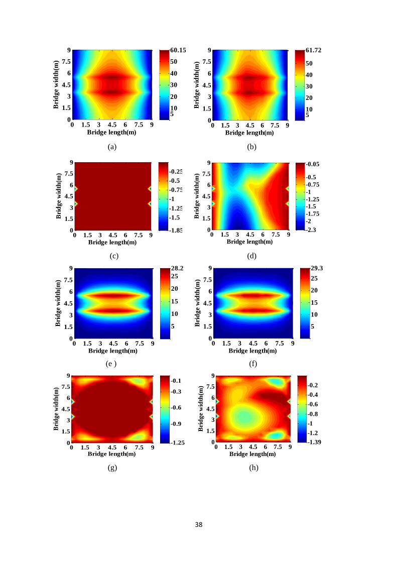
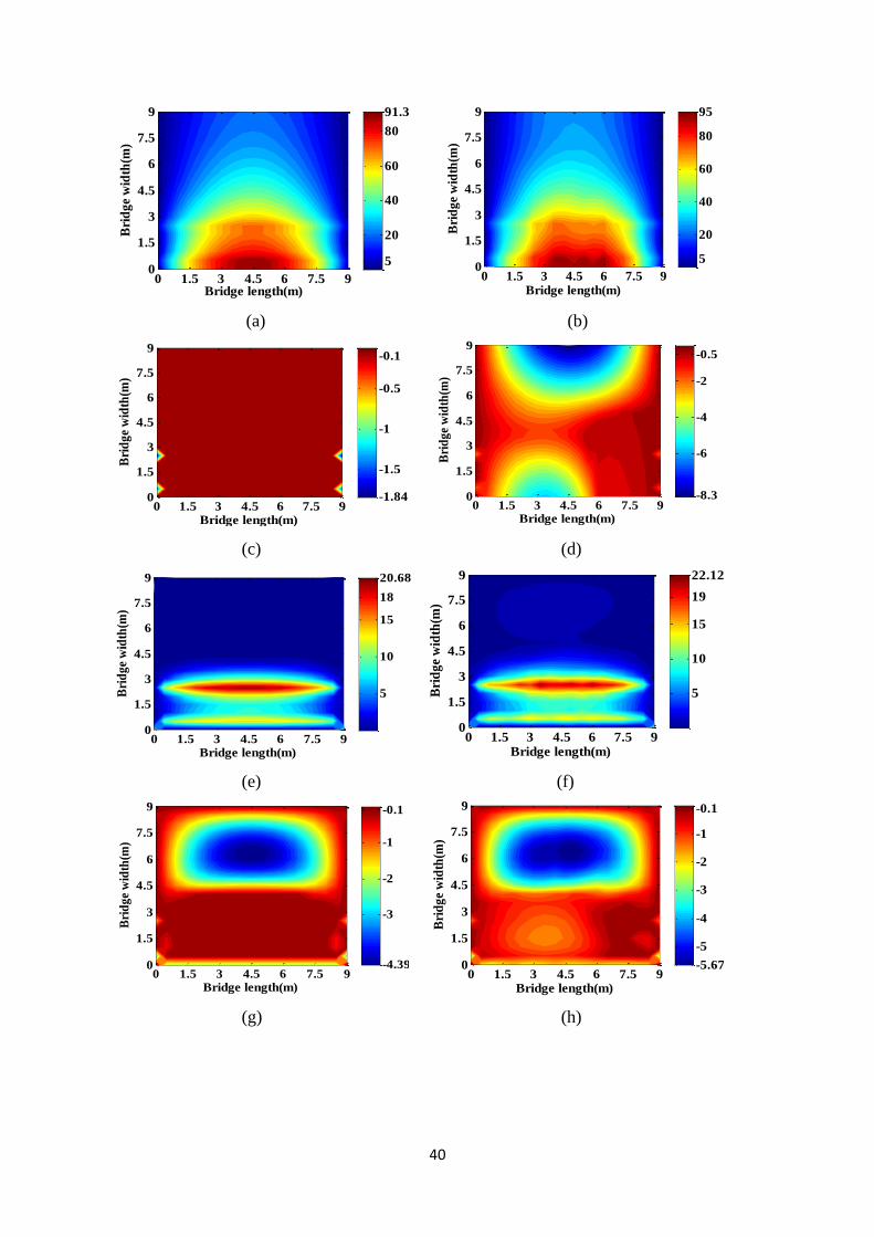
and the other two vehicle paths, together with the values of mxy and my. Figures 6 to 8 provide

contour plots for these moments at every node for the three paths of the vehicle travelling at 20

14

m/s. Both positive (i.e., sagging) and negative (i.e., hogging) mx and my, as well as positive and

negative mxy, are shown in the contour plots. The horizontal and vertical axes indicate the

longitudinal and transverse coordinates respectively of the node in a plan view of the bridge,

and the values of the colours represent the moments in kNm/m at each node location. Different

contour shapes and values of local bending moments emerge as a result of changes in vehicle

paths.

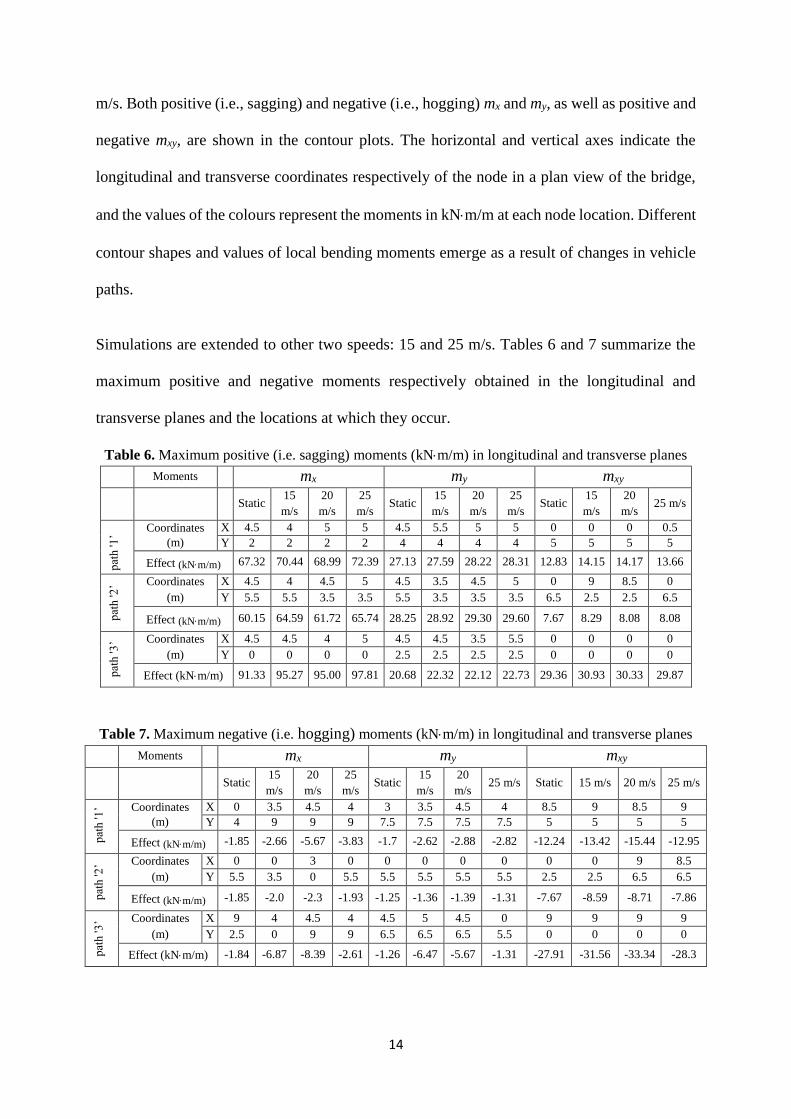
Simulations are extended to other two speeds: 15 and 25 m/s. Tables 6 and 7 summarize the

maximum positive and negative moments respectively obtained in the longitudinal and

transverse planes and the locations at which they occur.

Table 6. Maximum positive (i.e. sagging) moments (kNm/m) in longitudinal and transverse planes

Moments mx my mxy

Static 15

m/s

20

m/s

25

m/s Static

15

m/s

20

m/s

25

m/s Static

15

m/s

20

m/s 25 m/s

pat

h '1

’

Coordinates

(m)

X 4.5 4 5 5 4.5 5.5 5 5 0 0 0 0.5

Y 2 2 2 2 4 4 4 4 5 5 5 5

Effect (kNm/m) 67.32 70.44 68.99 72.39 27.13 27.59 28.22 28.31 12.83 14.15 14.17 13.66

pat

h '2

’ Coordinates

(m)

X 4.5 4 4.5 5 4.5 3.5 4.5 5 0 9 8.5 0

Y 5.5 5.5 3.5 3.5 5.5 3.5 3.5 3.5 6.5 2.5 2.5 6.5

Effect (kNm/m) 60.15 64.59 61.72 65.74 28.25 28.92 29.30 29.60 7.67 8.29 8.08 8.08

pat

h '3

’ Coordinates

(m)

X 4.5 4.5 4 5 4.5 4.5 3.5 5.5 0 0 0 0

Y 0 0 0 0 2.5 2.5 2.5 2.5 0 0 0 0

Effect (kNm/m) 91.33 95.27 95.00 97.81 20.68 22.32 22.12 22.73 29.36 30.93 30.33 29.87

Table 7. Maximum negative (i.e. hogging) moments (kNm/m) in longitudinal and transverse planes

Moments mx my mxy

Static 15

m/s

20

m/s

25

m/s Static

15

m/s

20

m/s 25 m/s Static 15 m/s 20 m/s 25 m/s

pat

h '1

’ Coordinates

(m)

X 0 3.5 4.5 4 3 3.5 4.5 4 8.5 9 8.5 9

Y 4 9 9 9 7.5 7.5 7.5 7.5 5 5 5 5

Effect (kNm/m) -1.85 -2.66 -5.67 -3.83 -1.7 -2.62 -2.88 -2.82 -12.24 -13.42 -15.44 -12.95

pat

h '2

’ Coordinates

(m)

X 0 0 3 0 0 0 0 0 0 0 9 8.5

Y 5.5 3.5 0 5.5 5.5 5.5 5.5 5.5 2.5 2.5 6.5 6.5

Effect (kNm/m) -1.85 -2.0 -2.3 -1.93 -1.25 -1.36 -1.39 -1.31 -7.67 -8.59 -8.71 -7.86

pat

h '3

’ Coordinates

(m)

X 9 4 4.5 4 4.5 5 4.5 0 9 9 9 9

Y 2.5 0 9 9 6.5 6.5 6.5 5.5 0 0 0 0

Effect (kNm/m) -1.84 -6.87 -8.39 -2.61 -1.26 -6.47 -5.67 -1.31 -27.91 -31.56 -33.34 -28.3

15

As expected, the maximum positive value of mx is considerably higher than the positive values

of my and mxy. While maximum positive mx occurs around the mid-span section, the maximum

positive my and maximum positive mxy develop under the wheel path and close to the supports

respectively. The exact transverse location of the maximum mxy varies with the vehicle path,

i.e., around the middle of the lane for path ‘2’ scenario (Figure 7) and at the bottom corner for

the path ‘3’ (Figure 8). As the path of the vehicle moves away from the bridge centreline, the

maximum longitudinal bending moment increases both in absolute value and in relative terms

compared to the maximum transverse bending moment. While maximum ‘static’ longitudinal

sagging and ‘static’ twisting moments of 91.33 and 29.36 kNm/m respectively take place for

path ‘3’, a maximum ‘static’ transverse sagging moment of 28.25 kNm/m takes place for path

‘2’. The maximum total longitudinal sagging moment is 35% and 49% higher for path ‘3’ than

for paths ‘1’ and ‘2’ respectively. The ratio of maximum longitudinal to maximum transverse

sagging moment is 2.22, 2.55 and 4.30 in vehicle paths ‘2’, ‘1’ and ‘3’ respectively.

The maximum negative values of bending moment (Table 7) are considerably smaller than the

positive values, but in the case of twisting moment, it is important to calculate both signs given

that the maximum twisting could take place in any of the two directions. The ratio of maximum

longitudinal sagging to maximum absolute twisting moment is 7.55, 4.69 and 2.93 in vehicle

paths ‘2’, ‘1’ and ‘3’ respectively. For path ‘3’, values of twisting moment exceed those of

transverse sagging moment. For path ‘2’, absolute ‘static’ values of negative and positive mxy

are naturally equal, but they vary slightly in the dynamic simulations due to randomness of the

road profile. Therefore, critical locations of maximum ‘static’ negative and positive mxy are

symmetrical with respect to the bridge centre line.

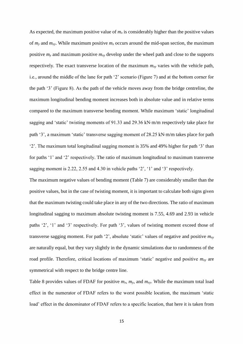
Table 8 provides values of FDAF for positive mx, my, and mxy. While the maximum total load

effect in the numerator of FDAF refers to the worst possible location, the maximum ‘static

load’ effect in the denominator of FDAF refers to a specific location, that here it is taken from

16

the worst possible static scenario given in Table 6 for positive values and in Table 7 for negative

values. The highest FDAF of positive bending moment for the three speeds being tested is 1.09

at 25 m/s, which takes place in path ‘2’ for the longitudinal plane and in path ‘3’ for the

transverse plane. A maximum FDAF of 1.10 is found for the positive twisting moment mxy

when the vehicle travels on path ‘1’ at speeds of 15 m/s and 20 m/s. A minimum FDAF of 1.01

is found for mxy, when the vehicle is travelling on path ‘3’ at a speed of 25 m/s.

Table 8. FDAF of positive (i.e. sagging) mx, my and mxy

FDAF of mx FDAF of my FDAF of mxy

Vehicle

path 15 m/s 20 m/s 25 m/s 15 m/s 20 m/s 25 m/s 15 m/s 20 m/s 25 m/s

path ‘1’ 1.04 1.02 1.07 1.01 1.04 1.04 1.10 1.10 1.06

path ‘2’ 1.07 1.02 1.09 1.02 1.03 1.04 1.08 1.05 1.05

path ‘3’ 1.04 1.04 1.07 1.07 1.06 1.09 1.05 1.03 1.01

Table 9 provides FDAF of hogging moments, which are generally much higher than those

provided in Table 8 for sagging ones. Nevertheless, the total hogging moment remains small

given the low values of maximum negative ‘static’ mx and my (Table 7).

Table 9. FDAF of negative (i.e. hogging) mx, my and mxy

FDAF of mx FDAF of my FDAF of mxy

Vehicle

path 15 m/s 20 m/s 25 m/s 15 m/s 20 m/s 25 m/s 15 m/s 20 m/s 25 m/s

path ‘1’ 1.44 3.06 2.07 1.54 1.69 1.66 1.10 1.26 1.06

path ‘2’ 1.08 1.24 1.04 1.09 1.11 1.05 1.12 1.14 1.02

path ‘3’ 3.73 4.56 1.42 5.13 4.5 1.04 1.13 1.19 1.02

In the case of twisting moments, FDAF of negative mxy should not be overlooked as mxy can

reach significant values with both signs. There is a FDAF of 1.26 for negative mxy when the

vehicle drives on path ‘1’ at 20 m/s. It is possible to define a global FDAF considering all

vehicle paths rather than use a FDAF for each path. For example, global FDAFs of 1.07, 1.05

and 1.14 can be obtained for longitudinal sagging, transverse sagging, and twisting moments

respectively. The next section extends the analysis of moments from the longitudinal and

17

transverse planes to any plane orientation. This analysis aims to stablish the bridge moment

capacity needed to withstand the applied total (‘static’ + ‘dynamic’) moment regardless of the

plane orientation.

4. Bending Moments Acting at any Plane

A slab deck has infinite points, and infinite number of planes passing through each point. This

section establishes the magnitude of the highest moments, and the node location and plane

orientation at which they occur. Figure 9 shows a plan view of the moments acting on a portion

of the slab delimited by three edges: BC of length L, AB of length Lcos, and AC of length

Lsin. AB, AC and BC are contained in planes of normal x, y and n respectively, and is the

angle between x- and n- directions. On each of these planes, there are two moments: a bending

moment (where the subscript denotes the direction of the normal to the plane on which the

moment is acting) that produces normal stresses, and a twisting moment (where the first and

second subscripts represent the direction of the normal to the plane on which the moment is

acting, and the direction of the shear stresses respectively) that produces shear stresses.

By imposing equilibrium of moments in the n-direction (Equation (10)) and in a direction

perpendicular to n (Equation (11)), it is possible to obtain the bending moment, mn, and twisting

moment, mnt, per unit breadth acting on a plane of normal n [4,26].

𝑚𝑛 = 𝑚𝑥 cos2𝜃 + 𝑚𝑦 sin2𝜃 − 2 𝑚𝑥𝑦 sin𝜃 cos𝜃 (10)

𝑚𝑛𝑡 = (𝑚𝑥 − 𝑚𝑦) sin𝜃 cos𝜃 + 𝑚𝑥𝑦(cos2𝜃 − sin2𝜃) (11)

where is the angle that the normal to the plane (n) makes with the horizontal x-axis.

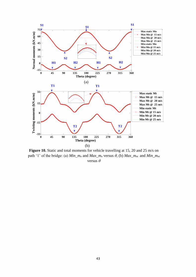
mx, my and mxy obtained in Section 3 are substituted into Equation (10) to calculate mn for every

node of the FE model. values are varied in 1 degree increment from 0 to 360°. The maximum

18

positive (Max_mn, i.e., sagging) and minimum negative (Min_mn, i.e., hogging) of ‘static’ and

total (15, 20 and 25 m/s) values of mn are plotted versus in Figure 10(a) for the vehicle

travelling on path ‘1’. Similarly, moments mx, my and mxy are replaced into Equation (11) to

obtain the maximum (Max_mnt) and minimum (Min_mnt) twisting moments per unit breadth

for every node. The latter are shown in Figure 10(b) for the vehicle travelling on path ‘1’.

Highest values of Max_mn take place at longitudinal planes ( values of 0°, 180° and 360° -

points labelled ‘S1’ in the figure -), whereas minimum values of Max_mn are found at

transverse planes ( values of 90° and 270° - points labelled ‘S2’-). Minimum values of Min_mn

develop for planes at 45° with horizontal and vertical planes ( values of 45° and 225 - points

labelled ‘H1’ -, and 225° and 315° - points labelled ‘H2’ -). Figure 10(b) shows that the most

positive and most negative twisting moments also occur in planes at 45° with horizontal and

vertical planes ( values of 45° and 225° for largest positive mnt - points labelled ‘T1’ -, and

values of 135° and 315° for largest negative mnt - points ‘T2’ -). In summary, longitudinal and

transverse bending moments are the maximum and minimum bending moments respectively.

Besides, critical twisting moments occur in planes at 45 with respect to the longitudinal and

transverse planes.

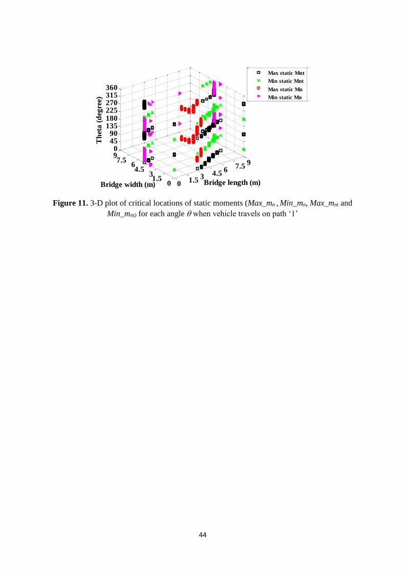
Figure 11 shows a 3-dimensional plot that locates the FE node that leads to maximum ‘static’

bending moments (negative ‘Min_mn’ labelled as purple triangles and positive ‘Max_mn’

labelled as red circles) and maximum ‘static’ twisting moments (maximum ‘Max_mnt’ labelled

as black squares and minimum ‘Min_mnt’ labelled as green crosses) for each plane orientation

. The locations holding these maximum and minimum moments vary for each value, but are

placed predominantly around midspan for Max_mn, and spread throughout the bridge for

Min_mn, Max_mnt and Min_mnt. The largest sagging moment occur in a longitudinal plane at

or near midspan, where the bending curvature of the deflected shape is highest. Bending

curvatures in other directions also increase the closer to midspan. For twisting and hogging

19

moments, the critical locations for each plane orientation are more variable due to the influence

of local effects. Maximum hogging appears in the half of the bridge where the vehicle is not

travelling, and largest absolute twisting moments tend to be found near the edges at midspan

and in the corners.

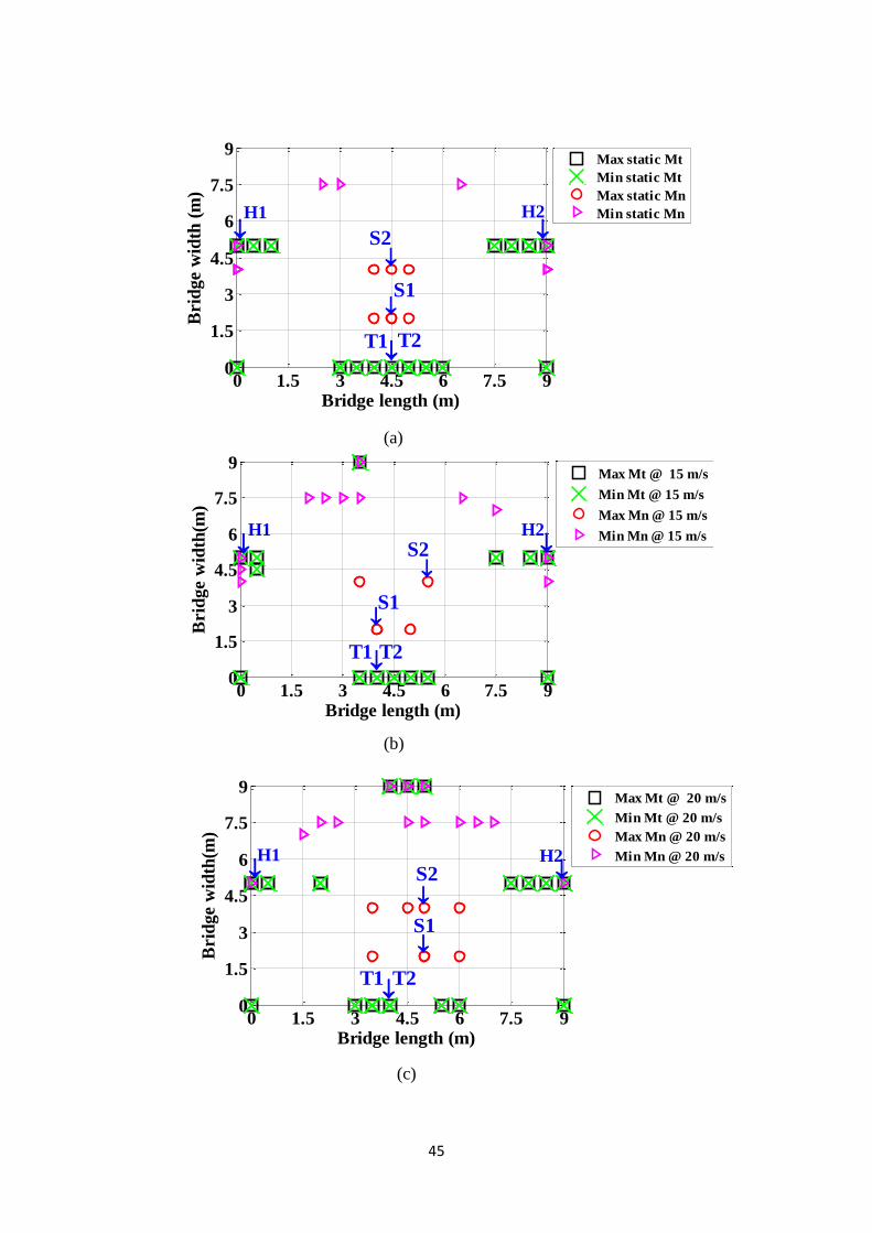
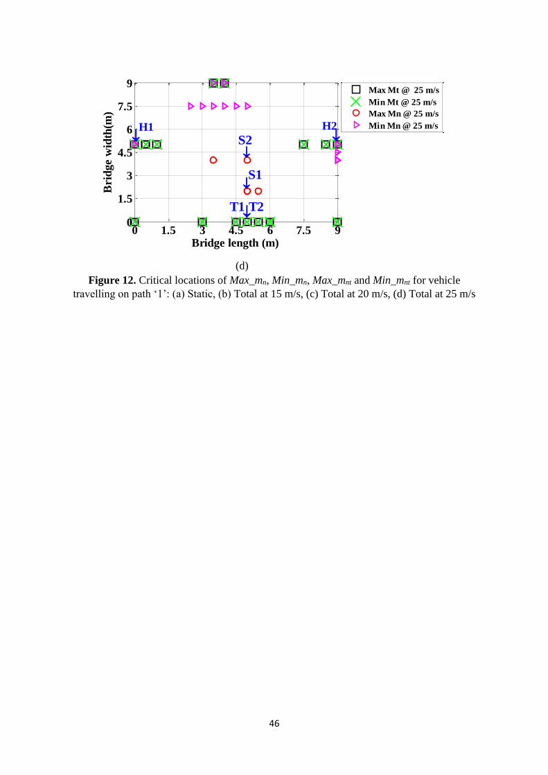
The coordinates of the critical locations cannot be clearly visualized in the 3-dimensional graph

of Figure 11. For this reason, horizontal sections for orientations equal to 45°, 90°,135° and

180° holding maximum ‘static’ and total moments are obtained. Figure 12 provides the X-

(horizontal axis, i.e. bridge span length) and Y- (vertical axis, i.e. bridge width) coordinates of

the critical locations for the four selected orientations, and how they vary with speed. For

instance, Figures 12(b) for 15 m/s and 12(d) for 25 m/s show 4 red circles which represent the

critical locations holding the maximum sagging for plane orientations equal to 45°, 90°, 135°

and 180°. However, Figures 12(a) (‘static’) and 12(c) for 20 m/s show 6 red circles, given that

the maximum sagging is reached at more than one critical location for some orientations. Here,

the points ‘S1’ (at Ɵ values of 0°, 180° and 360° in Figure 10(a)), ‘S2’ (at Ɵ values of 90°

and 270°), ‘H1’ (at Ɵ values of 45° and 225°) and ‘H2’ (at Ɵ values of 135° and 315°)

represent the locations with maximum and minimum sagging and hogging moments. Point ‘T1’

corresponds to the coordinates of the largest positive twisting moment (Max_mnt at = 45° and

225° in Figure 10(b)) and ‘T2’ to the largest negative twisting moment (Min_mnt at = 135°

and 225° in Figure 10(b)). It can be seen that maximum sagging moments develop near the

mid-span section in the half of the bridge traversed by the vehicle. The largest sagging moment

for path ‘1’ takes place at coordinates X = 5 m and Y = 2 m for a speed of 25 m/s (point S1 in

Figure 12(d)). The ‘dynamic’ component of the total response will not reach a peak

simultaneously with the ‘static’ component at midspan, except for a critical speed causing a

high DAF. As a result, the locations of maximum total sagging moments (Figures 12(b), (c)

20

and (d)) appear more scattered than the locations of maximum ‘static’ sagging moments (Figure

12(a)).

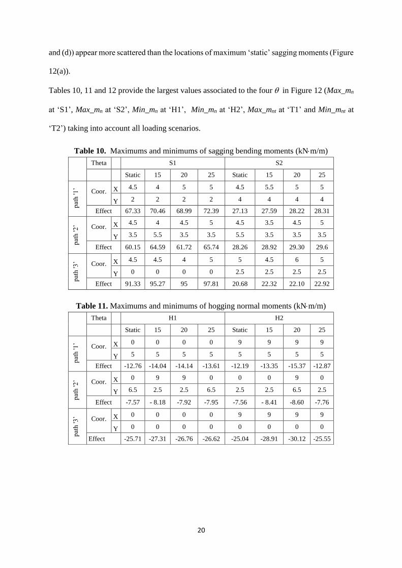
Tables 10, 11 and 12 provide the largest values associated to the four in Figure 12 (Max_mn

at ‘S1’, Max_mn at ‘S2’, Min_mn at ‘H1’, Min_mn at ‘H2’, Max_mnt at ‘T1’ and Min_mnt at

‘T2’) taking into account all loading scenarios.

Table 10. Maximums and minimums of sagging bending moments (kNm/m)

Theta S1 S2

Static 15 20 25 Static 15 20 25

pat

h '1

’

Coor. X 4.5 4 5 5 4.5 5.5 5 5

Y 2 2 2 2 4 4 4 4

Effect 67.33 70.46 68.99 72.39 27.13 27.59 28.22 28.31

pat

h '2

’ Coor. X 4.5 4 4.5 5 4.5 3.5 4.5 5

Y 3.5 5.5 3.5 3.5 5.5 3.5 3.5 3.5

Effect 60.15 64.59 61.72 65.74 28.26 28.92 29.30 29.6

pat

h '3

’ Coor. X 4.5 4.5 4 5 5 4.5 6 5

Y 0 0 0 0 2.5 2.5 2.5 2.5

Effect 91.33 95.27 95 97.81 20.68 22.32 22.10 22.92

Table 11. Maximums and minimums of hogging normal moments (kNm/m)

Theta H1 H2

Static 15 20 25 Static 15 20 25

pat

h '1

’

Coor. X 0 0 0 0 9 9 9 9

Y 5 5 5 5 5 5 5 5

Effect -12.76 -14.04 -14.14 -13.61 -12.19 -13.35 -15.37 -12.87

pat

h '2

’ Coor. X 0 9 9 0 0 0 9 0

Y 6.5 2.5 2.5 6.5 2.5 2.5 6.5 2.5

Effect -7.57 - 8.18 -7.92 -7.95 -7.56 - 8.41 -8.60 -7.76

pat

h '3

’ Coor. X 0 0 0 0 9 9 9 9

Y 0 0 0 0 0 0 0 0

Effect -25.71 -27.31 -26.76 -26.62 -25.04 -28.91 -30.12 -25.55

21

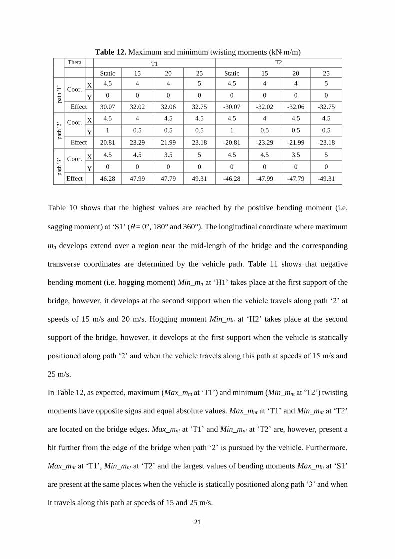
Table 12. Maximum and minimum twisting moments (kNm/m)

Theta T1 T2

Static 15 20 25 Static 15 20 25

pat

h '1

’

Coor. X 4.5 4 4 5 4.5 4 4 5

Y 0 0 0 0 0 0 0 0

Effect 30.07 32.02 32.06 32.75 -30.07 -32.02 -32.06 -32.75

pat

h '2

’ Coor. X 4.5 4 4.5 4.5 4.5 4 4.5 4.5

Y 1 0.5 0.5 0.5 1 0.5 0.5 0.5

Effect 20.81 23.29 21.99 23.18 -20.81 -23.29 -21.99 -23.18

pat

h '3

’ Coor. X 4.5 4.5 3.5 5 4.5 4.5 3.5 5

Y 0 0 0 0 0 0 0 0

Effect 46.28 47.99 47.79 49.31 -46.28 -47.99 -47.79 -49.31

Table 10 shows that the highest values are reached by the positive bending moment (i.e.

sagging moment) at ‘S1’ ( = 0°, 180° and 360°). The longitudinal coordinate where maximum

mn develops extend over a region near the mid-length of the bridge and the corresponding

transverse coordinates are determined by the vehicle path. Table 11 shows that negative

bending moment (i.e. hogging moment) Min_mn at ‘H1’ takes place at the first support of the

bridge, however, it develops at the second support when the vehicle travels along path ‘2’ at

speeds of 15 m/s and 20 m/s. Hogging moment Min_mn at ‘H2’ takes place at the second

support of the bridge, however, it develops at the first support when the vehicle is statically

positioned along path ‘2’ and when the vehicle travels along this path at speeds of 15 m/s and

25 m/s.

In Table 12, as expected, maximum (Max_mnt at ‘T1’) and minimum (Min_mnt at ‘T2’) twisting

moments have opposite signs and equal absolute values. Max_mnt at ‘T1’ and Min_mnt at ‘T2’

are located on the bridge edges. Max_mnt at ‘T1’ and Min_mnt at ‘T2’ are, however, present a

bit further from the edge of the bridge when path ‘2’ is pursued by the vehicle. Furthermore,

Max_mnt at ‘T1’, Min_mnt at ‘T2’ and the largest values of bending moments Max_mn at ‘S1’

are present at the same places when the vehicle is statically positioned along path ‘3’ and when

it travels along this path at speeds of 15 and 25 m/s.

22

Table 13 gives the FDAF for sagging moments Max_mn at ‘S2’ and Max_mn at ‘S1’.

Table 13. FDAF of sagging bending moments

FDAF FDAF of mn at ‘S1’ FDAF of mn at ‘S2’

Path 15 m/s 20 m/s 25 m/s 15 m/s 20 m/s 25 m/s

path ‘1’ 1.04 1.02 1.07 1.01 1.04 1.04

path ‘2’ 1.07 1.02 1.09 1.02 1.03 1.04

path ‘3’ 1.04 1.04 1.07 1.07 1.06 1.09

Table 14 presents the FDAF for hogging moments Min_mn at ‘H1’ and Min_mn at ‘H2’.

Table 14. FDAF of hogging bending moments

FDAF FDAF of mn at ‘H1’ FDAF of mn at ‘H2’


path ‘1’ 1.1 1.11 1.07 1.09 1.26 1.05

path ‘2’ 1.08 1.05 1.05 1.11 1.13 1.02

path ‘3’ 1.06 1.041 1.04 1.15 1.20 1.02

Table 15 gives the FDAF for twisting moments Max_mnt at ‘T1’ and Min_mnt at ‘T2’.

Table 15. FDAF of maximum and minimum twisting moments (kNm/m)

FDAF FDAF of mnt at ‘T1’ FDAF of mnt at ‘T2’


path ‘1’ 1.06 1.06 1.09 1.06 1.06 1.09

path ‘2’ 1.12 1.05 1.11 1.12 1.05 1.11

path ‘3’ 1.03 1.03 1.06 1.03 1.03 1.06

The majority of FDAF values for twisting moments and hogging moments are larger than those

of sagging moments (Max_mn at ‘S1’ and ‘S2’). The largest FDAF value is 1.26 for hogging

bending moment Min_mn at ‘H2’ when the vehicle is travelling on path ‘1’ at 20 m/s.

On the one hand, the critical sagging moment mn at ‘S1’ in Table 13 has the same associated

FDAFs than mx in Table 8, the reason being that the plane with largest sagging moment is the

longitudinal plane. Similarly, the sagging moment mn at ‘S2’ refers to the transverse plane, and

consequently, it has the same FDAFs as my in Table 8. On the other hand, FDAFs at ‘T1’ and

‘T2’ (at 45 with vertical and horizontal planes) in Table 15 are different from FDAFs for mxy

in Table 8, given that they refer to different planes. Largest FDAF associated to mnt ( = 45)

is 1.12.

23

The location, amount and strength of steel reinforcement and the section dimensions will

determine the moment capacity of the bridge in kNm/m. The latter must have a value

exceeding the applied moment. If orthogonal reinforcement was to be provided in X- and Y-

directions, i.e., mx* and my*, it is necessary to ensure that moment capacities in other directions

are also sufficiently large to prevent failure. For this purpose, the moment capacity at any plane

mn* can be estimated from replacing mn by mn*, mx by mx*, my by my* and mxy by 0 in Equation

(10), leading to ‘mx* = mx + mxy’ and ‘my* = my + mxy’. For example, the values of the sagging

capacities in longitudinal and transverse planes needed to withstand moments caused by the

vehicle travelling in path ‘1’ at 25 m/s are estimated next for the point X = 5 m and Y = 2 m

(where the maximum longitudinal bending moment of mx = 72.39 kNm/m takes place). The

contour plot in Figure 13(a) illustrates the variation of bending moment at this point with plane

orientation for each point in time (t = 0 seconds when the first axle of the truck is at the entrance

support). A concentration of high bending moments takes place for t = 0.57 seconds. Figure

13(b) shows how the capacities ‘mx* = mx + mxy’ and ‘my* = my + mxy’ required at the point

(X = 5 m, Y = 2 m) vary with mx, my and mxy for each instant. Maximum bending capacities of

mx* = 73.37 kNm/m and of my*= 27.33 kNm/m are necessary to withstand the moments

experienced at t = 0.57 seconds. While only the action of the vehicle is investigated in this

paper, combinations of actions (i.e., including self-weight) need to be taken into consideration

when calculating Max_mn in a practical situation. Other vehicle paths and a full range of

potential speeds (i.e., including critical speeds causing highest DAFs) also need to be checked

to ensure mx* and my* cover all possible failure scenarios.

5. Conclusions

This paper has investigated how a moving vehicle affects the ‘static’ and total moment acting

on any plane orientation of a short-span straight solid slab bridge. The crossing of a 5-axle

24

articulated truck over a FE plate model of the bridge on a class ‘A’ road carpet has been

simulated for nine loading scenarios including three vehicle speeds (15, 20 and 25 m/s) and

three transverse paths. For all scenarios, positive and negative bending and twisting moments

per unit breadth have been obtained in longitudinal and transverse planes. It has been found

that longitudinal sagging (mx) exhibits considerably larger values than transverse sagging (my)

or twisting (mxy). Maximum values occur most frequently over the middle portion of the bridge

for mx, over the bridge centreline for my, and at the bridge edges for mxy. Bridge codes such as

the Eurocode, propose traffic load models with built-in DAFs that quantify the increase that

the total response experiences as a result of dynamic VBI. For a two-lane 9 m bridge, this DAF

value is 1.26 [21]. However, built-in DAFs are necessarily conservative and do not allow for

changes in DAF for different moments. For the bridge scenarios under investigation, FDAF of

mx and my in sagging have had similar values with a maximum of 1.09 (vehicle travelling at 25

m/s, either along middle of the bridge for worst mx or partially on the shoulder for worst my),

but a maximum FDAF of negative mxy have reached 1.26 (vehicle travelling at 20 m/s along

the middle of the lane).

Furthermore, total (‘static’ + ‘dynamic’) bending (mn) and twisting (mnt) moments acting on

any plane of normal n have been analysed. From the point of view of sagging moments, the

plane orientations leading to largest values have taken place at longitudinal planes, i.e.,

largest Max_mn = mx. The plane orientations leading to smallest values of Max_mn have

occurred at transverse planes, i.e., smallest Max_mn = my. Largest values of hogging and

twisting moments have developed at 45° with respect to longitudinal and transverse planes.

Even though bending moments will be largest at longitudinal planes, this paper has shown that

bending failure may occur at orientations other than longitudinal. Therefore, the maximum total

applied moment (Max_mn) must be calculated and compared to the available moment capacity

of the bridge (mn*) for every plane orientation. An accurate assessment taking into account

25

these subtleties is clearly justified if an existing bridge could be saved from unnecessary

strengthening or replacing.

ACKNOWLEDGEMENTS

The authors wish to express their gratitude for the financial support received from Al-Anbar

University and Iraqi ministry of higher education towards this research.

References

[1] DIVINE. Dynamic interaction of heavy vehicles with roads and bridges, Canada. DIVINE

Concluding Conference; OCED; Ottawa; Technical report; 1997.

[2] OBrien EJ, Cantero D, Enright B, González A. Characteristic Dynamic Increment for extreme

traffic loading events on short and medium span highway bridges. Eng Struct 2010;32:3827–

35.

[3] Tarmac. Prestressed beams technical guide 2009.

[4] Wood RH. The Reinforcement of Slabs in Accordance with a Pre-Determined Field of

Moments. Concrete 1968;2:69–76.

[5] Zararis PD. State of Stress in RC Plates under Service Conditions. J Struct Eng

1986;112:1908–27.

[6] Zararis PD. Failure Mechanisms in R/C Plates Carrying In‐Plane Forces. J Struct Eng

1988;114:553–74.

[7] Ghoneim MG, MacGregor JG. Behavior of Reinforced Concrete Plates Under Combined

Inplane and Lateral Loads. Struct J 1994;91:188–97.

[8] Ghoneim MG, Macgregor JG. Prediction of the Ultimate Strength of Reinforced Concrete

Plates Under Combined Inplane and Lateral Loads. Struct J 1994;91:688–96.

[9] Ghoneim MG, McGregor JG. Tests of Reinforced Concrete Plates Under Combined Inplane

and Lateral Loads. Struct J 1994;91:19–30.

[10] Frýba L. Vibration of solids and structures under moving loads. Groningen, The Netherlands:

Noordhoff International Publishing; 1972.

26

[11] Bakht B, Pinjarkar S. G. Dynamic testing of highway bridges—A review. Transportation

Research Record 1223, Transportation Research Board, Washington, DC, 93–100. 1989.

[12] Inbanathan MJ, Wieland M. Bridge Vibrations Due to Vehicle Moving Over Rough Surface. J

Struct Eng 1987;113:1994–2008.

[13] Wang W, Deng L, Asce M. Impact Factors for Fatigue Design of Steel I-Girder Bridges

Considering the Deterioration of Road Surface Condition. J Bridg Eng 2016;21:04016011.

[14] Park YS, Shin DK, Chung TJ. Influence of road surface roughness on dynamic impact factor

of bridge by full-scale dynamic testing. Can J Civ Eng 2005;829:825–9.

[15] Senthilvasan J, Thambiratnam D., Brameld G. Dynamic response of a curved bridge under

moving truck load. Eng Struct 2002;24:1283–93.

[16] Moghimi H, Ronagh HR. Impact factors for a composite steel bridge using non-linear dynamic

simulation. Int J Impact Eng 2008;35:1228–43.

[17] Rezaiguia A, Ouelaa N, Laefer DFF, Guenfoud S. Dynamic amplification of a multi-span,

continuous orthotropic bridge deck under vehicular movement. Eng Struct 2015;100:718–30.

[18] Mohammed O, Cantero D, González A, Al-Sabah S. Dynamic amplification factor of

continuous versus simply supported bridges due to the action of a moving load, Civil

engineering research in Ireland (CERI 2014) , Queen’s Univ, Belfast, 28-29 August, 2014.

2014-08-29: 2014.

[19] Pesterev AV, Bergman LA, Tan CA, Yang B. Application of the pothole DAF method to

vehicles traversing periodic roadway irregularities. J Sound Vib 2005;279:843–55.

[20] Cantero D, González A, OBrien EJ. Maximum dynamic stress on bridges traversed by moving

loads. Proc ICE - Bridg Eng 2009;162:75–85.

[21] González A, Cantero D, OBrien EJ. Dynamic increment for shear force due to heavy vehicles

crossing a highway bridge. Comput Struct 2011;89:2261–72.

[22] Zienkiewicz OC, Taylor RL, Zhu JZ, OCZ, Rlt, Jzz. The Finite Element Method Set. Elsevier;

2005.

[23] Reddy JN. Energy Principles and Variational Methods in Applied Mechanics. John Wiley &

Sons; 2002.

[24] Bonger FK, Fox RL, Schmit LA. The generation of inter-element-compatible stiffness and

mass matrices by the use of interpolation formulas. Proceeding’s 1st Conf. matrix methods

Struct. Mech. Air Force Inst Tech, Wright Patterson A.F. Base, Ohio, 397-443, 1965.

27

[25] Rowley C. Moving force identification of axle forces in bridges. PhD thesis. School Civ Eng,

University College Dublin, Ireland, 2007.

[26] OBrien EJ, Keogh D, O,Connor A. Bridge deck Analysis. CRC Press ; 2015.

[27] Li YC. Factors affecting the dynamic interaction of bridges and vehicle loads. PhD Thesis,

Dep Civ Eng, University College Dublin,Ireland, 2006.

[28] Clough RW and Penzien J. Dynamics of structures. 2nd editio. McGraw-Hil; 1993.

[29] Cantero D, González A, OBrien EJ. Comparison of bridge dynamic amplification due to

articulated 5-axle trucks and large cranes. Balt J Road Bridg Eng 2011;6:39–47.

[30] Cebon D. Handbook of vehicle-road interaction. Swets & Zeitlinger Lisse, The Netherlands;

1999.

[31] González A, OBrien EJ, Cantero D, Li Y, Dowling J, Žnidarič A. Critical speed for the

dynamics of truck events on bridges with a smooth road surface. J Sound Vib 2010;329:2127–

46. doi:10.1016/j.jsv.2010.01.002.

[32] Deng L, Cai CSS. Development of dynamic impact factor for performance evaluation of

existing multi-girder concrete bridges. Eng Struct 2010;32:21–31.

[33] Kim C-W, Kawatani M, Kwon Y-R. Impact coefficient of reinforced concrete slab on a steel

girder bridge. Eng Struct 2007;29:576–90.

[34] Broquet C, Bailey SF, Fafard M, Brühwiler E. Dynamic behavior of deck slabs of concrete

road bridges. J Bridg Eng, 9 (2) (2004), pp. 137–146.

[35] Huang DZ, Wang TL, Shahawy M. Dynamic behavior of horizontally curved I-girder bridges.

Comput Struct 1995;57:703–14.

[36] Huang DZ, Wang TL, Shahawy M. Impact analysis of continuous multigirder bridges due to

moving vehicles. J Struct Eng 1992;118:3427–43.

[37] Cebon D, Newland DE. Artificial generation of road surface topography by the inverse FFT

method. Veh Syst Dyn 1983;12:160–5.

[38] ISO 8608:1995, Mechanical Vibration-road Surface Profiles-reporting of Measured Data’,

International Standards Organisation. 1995.

[39] Keenahan J, OBrien EJ, McGetrick PJ, Gonzalez A. The use of a dynamic truck-trailer drive-

by system to monitor bridge damping. Struct Heal Monit 2013;13:143–57.

[40] Harris NK, OBrien EJ, González A. Reduction of bridge dynamic amplification through

28

adjustment of vehicle suspension damping. J Sound Vib 2007;302:471–85.

[41] Sayers M, Karamihas S. Interpretation of road roughness profile data. Tech rep, Univ of

Michigan Transportation Research Institute (UMTRI) Report 96–19, 1996.

[42] Green MF, Cebon D. Dynamic interaction between heavy vehicles and highway bridges.

Comput Struct 1997;62:253–64.

[43] Cantero D, OBrien EJ, González A. Modelling the vehicle in vehicle-infrastructure dynamic

interaction studies. Proc Inst Mech Eng Part K J Multi-Body Dyn 2010;224:243–8.

29

Figure captions:

Figure 1. Moments acting on longitudinal and transverse planes of plate element with four

nodes

Figure 2. General vehicle model sketch: (a) Side view, (b) Front view (Symbols defined in

Table 3)

Figure 3. Road profile carpet

Figure 4. Plan view showing location of vehicle paths on bridge plate model

Figure 5: Longitudinal bending moment per unit breadth mx: (a) Total and static mx versus

truck location for node at 3.5 m from left edge of the bridge, (b) Total and static mx versus

truck location for node at right edge of the bridge, (c) Envelope of maximum static and total

mx at section A-A.

Figure 6. Envelope of maximum positive and negative moments for vehicle travelling on

path ‘1’ of the bridge at 20 m/s: (a) Maximum static positive mx (kNm/m), (b) Maximum

total positive mx (kNm/m), (c) Maximum static negative mx (kNm/m), (d) Maximum total

negative mx (kNm/m), (e) Maximum static positive my (kNm/m), (f) Maximum total positive

my (kNm/m), (g) Maximum static negative my (kNm/m), (h) Maximum total negative my

(kNm/m), (i) Maximum static positive mxy (kNm/m), (j) Maximum total positive mxy

(kNm/m), (k) Maximum static negative mxy (kNm/m), (l) Maximum total negative mxy

(kNm/m)








(kNm/m)




30





(kNm/m)

Figure 9. Plan view of moments acting on a plate slice

Figure 10. Static and total moments for vehicle travelling at 15, 20 and 25 m/s on path ‘1’ of

the bridge: (a) Min_mn and Max_mn versus , (b) Max_mnt and Min_mnt versus

Figure 11. 3-D plot of critical locations of static moments (Max_mn , Min_mn, Max_mnt and

Min_mnt) for each angle when vehicle travels on path ‘1’

Figure 12. Critical locations of Max_mn, Min_mn, Max_mnt and Min_mnt for vehicle travelling

on path ‘1’: (a) Static, (b) Total at 15 m/s, (c) Total at 20 m/s, (d) Total at 25 m/s

Figure 13. Moments acting on point of coordinates (X = 5 m,Y = 2 m) due to the vehicle

travelling along path ‘1’ at 25 m/s: (a) Bending moment mn versus time and plane orientation

(0 to 360 degrees), (b) mx, my, mxy, mx* and my* versus time

31

Figure 1. Moments acting on longitudinal and transverse planes of plate element

with four nodes

32

(a) (b)

Figure 2. General vehicle model sketch: (a) Side view, (b) Front view (Symbols defined in

Table 3)

33

Figure 3. Road profile carpet

34

( ) Centreline of the vehicle

Figure 4. Plan view showing location of vehicle paths on bridge plate model

35

(a) (b)

(c)

Figure 5. Longitudinal bending moment per unit breadth mx: (a) Total and static mx versus

truck location for node at 3.5 m from left edge of the bridge, (b) Total and static mx versus

truck location for node at right edge of the bridge, (c) Envelope of maximum static and

total mx at section A-A.

0 5 10 15 20-5

20

40

60

70

Position of 1st axle from bridge 1st support (m)

mx (

kN

.m/m

)

Total

Static

0 5 10 15 20-5

5

15

25

35

45

Position of 1st axle from bridge 1st support (m)

mx (

kN

.m/m

)

Total

Static

0 1 2 3 4 5 6 7 8 940

45

50

55

60

65

Distance to left edge (m)

mx (

kN

.m/m

)

Transverse midspan BM when 2nd axle at midspan

Static

TotalLocation: 3.5 m

Left edge Right edge

36

(a) (b)

(c) (d)

(e) (f)

(g) (h)

Bridge length(m)

Bri

dg

e w

idth

(m)

static Mx 1st path

0 1.5 3 4.5 6 7.5 90

1.5

3

4.5

6

7.5

9

10

20

30

40

50

6067.33

Bridge length(m)

Bri

dg

e w

idth

(m)

Total Mx 1st path

0 1.5 3 4.5 6 7.5 90

1.5

3

4.5

6

7.5

9

10

20

30

40

50

60

68.99

Bridge length(m)

Bri

dg

e w

idth

(m)

Static negative Mx 1st path

0 1.5 3 4.5 6 7.5 90

1.5

3

4.5

6

7.5

9

-1.85

-1.5

-1

-0.5

-0.1

Bridge length(m)

Bri

dg

e w

idth

(m)

Total negative Mx 1st path

0 1.5 3 4.5 6 7.5 90

1.5

3

4.5

6

7.5

9

-5.67

-5

-4

-3

-2

-1

Bridge length(m)

Bri

dg

e w

idth

(m)

Static My 1st path

0 1.5 3 4.5 6 7.5 90

1.5

3

4.5

6

7.5

9

5

10

15

20

27.13

Bridge length(m)

Bri

dg

e w

idth

(m)

Total My 1st path

0 1.5 3 4.5 6 7.5 90

1.5

3

4.5

6

7.5

9

5

10

15

20

28.22

Bridge length(m)

Bri

dg

e w

idth

(m)

Static negative My 1st path

0 1.5 3 4.5 6 7.5 90

1.5

3

4.5

6

7.5

9

-1.69

-1.5

-1.25

-1

-0.75

-0.5

-0.25

Bridge length(m)

Bri

dg

e w

idth

(m)

Total negative My 1st path

0 1.5 3 4.5 6 7.5 90

1.5

3

4.5

6

7.5

9

-2.88

-2.5

-2

-1.5

-1

-0.5-0.25

37

(i) ( j )

(k) (l)



total positive mx (kNm/m), (c) Maximum static negative mx (kNm/m), (d) Maximum

total negative mx (kNm/m), (e) Maximum static positive my (kNm/m), (f) Maximum total

positive my (kNm/m), (g) Maximum static negative my (kNm/m), (h) Maximum total

negative my (kNm/m), (i) Maximum static positive mxy (kNm/m), (j) Maximum total

positive mxy (kNm/m), (k) Maximum static negative mxy (kNm/m), (l) Maximum total

negative mxy (kNm/m)

Bridge length(m)

Bri

dg

e w

idth

(m)

Static Mxy 1st path

0 1.5 3 4.5 6 7.5 90

1.5

3

4.5

6

7.5

9

2

4

6

8

10

12.83

Bridge length(m)

Bri

dg

e w

idth

(m)

Total Mxy 1st path

0 1.5 3 4.5 6 7.5 90

1.5

3

4.5

6

7.5

9

2

4

6

8

10

12

14.17

Bridge length(m)

Bri

dg

e w

idth

(m)

Static negative Mxy 1st path

0 1.5 3 4.5 6 7.5 90

1.5

3

4.5

6

7.5

9

-12.24

-10

-8

-6

-4

-2

Bridge length(m)

Bri

dg

e w

idth

(m)

Total negative Mxy 1st path

0 1.5 3 4.5 6 7.5 90

1.5

3

4.5

6

7.5

9

-15.2

-13.5-12

-10

-8

-6

-4

-2

38

(a) (b)

(c) (d)

(e ) (f)

(g) (h)

Bridge length(m)

Bri

dg

e w

idth

(m)

Static Mx 2nd path

0 1.5 3 4.5 6 7.5 90

1.5

3

4.5

6

7.5

9

510

20

30

40

50

60.15

Bridge length(m)

Bri

dg

e w

idth

(m)

Total Mx 2nd path

0 1.5 3 4.5 6 7.5 90

1.5

3

4.5

6

7.5

9

510

20

30

40

50

61.72

Bridge length(m)

Bri

dg

e w

idth

(m)

Static negative Mx 2nd path

0 1.5 3 4.5 6 7.5 90

1.5

3

4.5

6

7.5

9

-1.85

-1.5

-1.25

-1

-0.75

-0.5

-0.25

Bridge length(m)

Bri

dg

e w

idth

(m)

Total negative Mx 2nd path

0 1.5 3 4.5 6 7.5 90

1.5

3

4.5

6

7.5

9

-2.3

-2

-1.75

-1.5-1.25

-1

-0.75

-0.5

-0.05

Bridge length(m)

Bri

dg

e w

idth

(m)

Static My 2nd path

0 1.5 3 4.5 6 7.5 90

1.5

3

4.5

6

7.5

9

5

10

15

20

25

28.2

Bridge length(m)

Bri

dg

e w

idth

(m)

Total My 2nd path

0 1.5 3 4.5 6 7.5 90

1.5

3

4.5

6

7.5

9

5

10

15

20

25

29.3

Bridge length(m)

Bri

dg

e w

idth

(m)

Static negative My 2nd path

0 1.5 3 4.5 6 7.5 90

1.5

3

4.5

6

7.5

9

-1.25

-0.9

-0.6

-0.3

-0.1

Bridge length(m)

Bri

dg

e w

idth

(m)

Total negative My 2nd path

0 1.5 3 4.5 6 7.5 90

1.5

3

4.5

6

7.5

9

-1.39

-1.2

-1

-0.8

-0.6

-0.4

-0.2

39

(i) ( j )

(k) (l)

Figure 7. Envelope of maximum positive and negative moments for vehicle

travelling on path ‘2’ of the bridge at 20 m/s: (a) Maximum static positive mx

(kNm/m), (b) Maximum total positive mx (kNm/m), (c) Maximum static negative

mx (kNm/m), (d) Maximum total negative mx (kNm/m), (e) Maximum static

positive my (kNm/m), (f) Maximum total positive my (kNm/m), (g) Maximum static

negative my (kNm/m), (h) Maximum total negative my (kNm/m), (i) Maximum

static positive mxy (kNm/m), (j) Maximum total positive mxy (kNm/m), (k)

Maximum static negative mxy (kNm/m), (l) Maximum total negative mxy (kNm/m)

Bridge length(m)

Bri

dg

e w

idth

(m)

Static Mxy 2nd path

0 1.5 3 4.5 6 7.5 90

1.5

3

4.5

6

7.5

9

0.5

2

4

6

7.67

Bridge length(m)

Bri

dg

e w

idth

(m)

Total Mxy 2nd path

0 1.5 3 4.5 6 7.5 90

1.5

3

4.5

6

7.5

9

2

4

6

8.08

Bridge length(m)

Bri

dg

e w

idth

(m)

Static negative Mxy 2nd path

0 1.5 3 4.5 6 7.5 90

1.5

3

4.5

6

7.5

9

-7.67

-6

-4

-2

-0.5

Bridge length(m)

Bri

dg

e w

idth

(m)

Total negative Mxy 2nd path

0 1.5 3 4.5 6 7.5 90

1.5

3

4.5

6

7.5

9

-8.7

-6

-4

-2

-0.5

40

(a) (b)

(c) (d)

(e) (f)

(g) (h)

Bridge length(m)

Bri

dg

e w

idth

(m)

Static Mx 3rd path

0 1.5 3 4.5 6 7.5 90

1.5

3

4.5

6

7.5

9

5

20

40

60

80

91.33

Bridge length(m)

Bri

dg

e w

idth

(m)

Total Mx 3rd path

0 1.5 3 4.5 6 7.5 90

1.5

3

4.5

6

7.5

9

5

20

40

60

80

95

Bridge length(m)

Bri

dg

e w

idth

(m)

Static negative Mx 3rd path

0 1.5 3 4.5 6 7.5 90

1.5

3

4.5

6

7.5

9

-1.84

-1.5

-1

-0.5

-0.1

Bridge length(m)

Bri

dg

e w

idth

(m)

Total negative Mx 3rd path

0 1.5 3 4.5 6 7.5 90

1.5

3

4.5

6

7.5

9

-8.3

-6

-4

-2

-0.5

Bridge length(m)

Bri

dg

e w

idth

(m)

Static My 3rd path

0 1.5 3 4.5 6 7.5 90

1.5

3

4.5

6

7.5

9

5

10

15

18

20.68

Bridge length(m)

Bri

dg

e w

idth

(m)

Total My 3rd path

0 1.5 3 4.5 6 7.5 90

1.5

3

4.5

6

7.5

9

5

10

15

19

22.12

Bridge length(m)

Bri

dg

e w

idth

(m)

Static negative My 3rd path

0 1.5 3 4.5 6 7.5 90

1.5

3

4.5

6

7.5

9

-4.39

-3

-2

-1

-0.1

Bridge length(m)

Bri

dg

e w

idth

(m)

Total negative My 3rd path

0 1.5 3 4.5 6 7.5 90

1.5

3

4.5

6

7.5

9

-5.67

-5

-4

-3

-2

-1

-0.1

41

(i) ( j )

(k) (l)

Figure 8. Envelope of maximum positive and negative moments for vehicle travelling

on path ‘3’ of the bridge at 20 m/s: (a) Maximum static positive mx (kNm/m), (b)

Maximum total positive mx (kNm/m), (c) Maximum static negative mx (kNm/m), (d)

Maximum total negative mx (kNm/m), (e) Maximum static positive my (kNm/m), (f)

Maximum total positive my (kNm/m), (g) Maximum static negative my (kNm/m), (h)

Maximum total negative my (kNm/m), (i) Maximum static positive mxy (kNm/m), (j)

Maximum total positive mxy (kNm/m), (k) Maximum static negative mxy (kNm/m), (l)

Maximum total negative mxy (kNm/m)

Bridge length(m)

Bri

dg

e w

idth

(m)

Static Mxy 3rd path

0 1.5 3 4.5 6 7.5 90

1.5

3

4.5

6

7.5

9

5

10

15

20

25

29.36

Bridge length(m)

Bri

dg

e w

idth

(m)

Total Mxy 3rd path

0 1.5 3 4.5 6 7.5 90

1.5

3

4.5

6

7.5

9

5

10

15

20

25

30.32

Bridge length(m)

Bri

dg

e w

idth

(m)

Static negative Mxy 3rd path

0 1.5 3 4.5 6 7.5 90

1.5

3

4.5

6

7.5

9

-27.91

-25

-20

-15

-10

-5

Bridge length(m)

Bri

dg

e w

idth

(m)

Total negative Mxy 3rd path

0 1.5 3 4.5 6 7.5 90

1.5

3

4.5

6

7.5

9

-33.34

-30

-25

-20

-15

-10

-5

42

Figure 9. Plan view of moments acting on a plate slice

43

(a)

(b)

Figure 10. Static and total moments for vehicle travelling at 15, 20 and 25 m/s on

path ‘1’ of the bridge: (a) Min_mn and Max_mn versus , (b) Max_mnt and Min_mnt

versus

0 45 90 135 180 225 270 315 360-15

0

15

30

45

60

75 S1

Theta (degree)

No

rma

l m

om

ents

(k

N.m

/m)

normal bending moments versus theta of the plane of 9X9 along the 1st path

Max static Mn

Max Mn @ 15 m/s

Max Mn @ 20 m/s

Max Mn @ 25 m/s

Min static Mn

Min Mn @ 15 m/s

Min Mn @ 20 m/s

Min Mn @ 25 m/s

S1 S1

S2S2

H1 H2 H1 H2

0 45 90 135 180 225 270 315 360-33

-15

0

15

33

Theta (degree)

Tw

isti

ng

mo

men

ts (

kN

.m/m

)

Twisting bending moments versus theta of the plane of 9X9 along the 1st path

Max static Mt

Max Mt @ 15 m/s

Max Mt @ 20 m/s

Max Mt @ 25 m/s

Min static Mt

Min Mt @ 15 m/s

Min Mt @ 20 m/s

Min Mt @ 25 m/s

T1 T1

T2 T2

44

Figure 11. 3-D plot of critical locations of static moments (Max_mn , Min_mn, Max_mnt and

Min_mnt) for each angle when vehicle travels on path ‘1’

01.5

3 4.56

7.59

01.5

34.5

67.5

90

4590

135180225270315360

Bridge length (m)

Loc of twis and norm mom vs theta plane of 9X9 1st path

Bridge width (m)

Th

eta

(d

egre

e)

Max static Mnt

Min static Mnt

Max static Mn

Min static Mn

45

(a)

(b)

(c)

0 1.5 3 4.5 6 7.5 90

1.5

3

4.5

6

7.5

9

T1 T2

S2

S1

H1

H2

Bridge length (m)

Brid

ge

wid

th (

m)

Loc of static twis and norm mom vs theta plane of 9X9 1st path

Max static Mt

Min static Mt

Max static Mn

Min static Mn

0 1.5 3 4.5 6 7.5 90

1.5

3

4.5

6

7.5

9

T1

S2

S1

H1

H2

Bridge length (m)

Brid

ge w

idth

(m)

Loc of totat @ 15 twis and norm mom vs theta plane of 9X9 1st path

T2

Max Mt @ 15 m/s

Min Mt @ 15 m/s

Max Mn @ 15 m/s

Min Mn @ 15 m/s

0 1.5 3 4.5 6 7.5 90

1.5

3

4.5

6

7.5

9

T1

S2

S1

H1

H2

Bridge length (m)

Bri

dge

wid

th(m

)


T2

Max Mt @ 20 m/s

Min Mt @ 20 m/s

Max Mn @ 20 m/s

Min Mn @ 20 m/s

46

(d)

Figure 12. Critical locations of Max_mn, Min_mn, Max_mnt and Min_mnt for vehicle

travelling on path ‘1’: (a) Static, (b) Total at 15 m/s, (c) Total at 20 m/s, (d) Total at 25 m/s

0 1.5 3 4.5 6 7.5 90

1.5

3

4.5

6

7.5

9

T1 T2

S2

S1

H1

H2

Bridge length (m)

Brid

ge w

idth

(m)


Max Mt @ 25 m/s

Min Mt @ 25 m/s

Max Mn @ 25 m/s

Min Mn @ 25 m/s

47

(a)

(b)

Figure 13. Moments acting on point of coordinates (X = 5 m,Y = 2 m) due to the

vehicle travelling along path ‘1’ at 25 m/s: (a) Bending moment mn versus time and

plane orientation (0 to 360 degrees), (b) mx, my, mxy, mx* and my* versus time

Time (s)

Th

eta

(d

eg

ree)

Normal Moment at single point

0 0.2 0.4 0.6 0.7720

45

90

135

180

225

270

315

360

0

20

40

60

72.39

0 0.2 0.4 0.6 0.772

0

20

40

60

80

Time(s)

Mo

men

t (k

N.m

/m)

NormalM

oment at single point

m

x

my

mxy

m*x

m*y

static and dynamic moments for any plane within a straight

Documents