Stated Choice design variables:Do they play a role on valuation estimates?

Subcommittee meetingTRB

Washington - 12th January, 2015

Manuel Ojeda Cabral

Research Fellow in Travel Behavior Modelling

Institute for Transport Studies, University of Leeds 1

Introduction: The value of a good

• Stated Choice experiments are a popular tool to estimate the value of a good.

• In transport economics: the Value of Travel Time

2

Assumption: We can find it in people’s choices that involve a trade-off

between money and time.

• Valuation of a good varies:• For different people

• Even for the same person

3

Introduction: The value of a good

Introduction: The value of a good

4

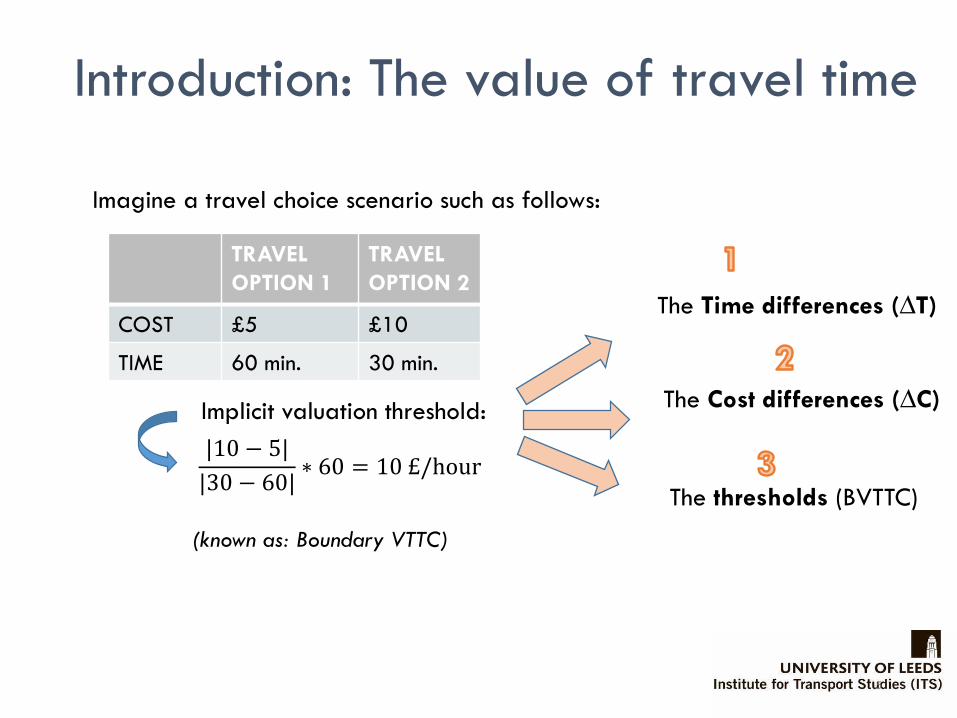
Imagine a travel choice scenario such as follows:

TRAVEL

OPTION 1

TRAVEL

OPTION 2

COST £5 £10

TIME 60 min. 30 min.

Implicit valuation threshold:

|10 − 5|

|30 − 60|∗ 60 = 10 £/hour

(known as: Boundary VTTC)

The thresholds (BVTTC)

The Time differences (∆T)

The Cost differences (∆C)

Introduction: The value of travel time

5

Objective: the role of SC design variables

• Stated Choice experiment

6

• Set of VTTC

𝐵𝑜𝑢𝑛𝑑𝑎𝑟𝑦𝑉𝑇𝑇𝐶 =∆𝐶𝑜𝑠𝑡

∆𝑇𝑖𝑚𝑒- Mean VTTC

- Income elasticity

- Distance elasticity

- Etc.

A) Influence of BVTTC, ∆T & ∆C: part of individuals’ true preferences? UNKNOWN. B) In any case, if model estimates are different in different settings, then by focussing the survey on specific settings, our sample level results will be affected accordingly.

Analysing the role of design variables

• SC design for many European VTTC studies:• Simple money-time trade-offs; 4 types:

7

Details on the UK design:

Design variable Values used for the SC experiment

Δt (minutes) -20, -15, -10, -5, -3, +5, +10, +15, +20

Δc (pence) -300, -250, -225, -150, -140, -125, -105, -100, -75, -70, -50, -35, -30, -25,-20, -15, -10, -5, 5, 10,

15, 20, 25, 30, 35, 50, 70, 75, 100, 105,125, 140, 150, 225, 250, 300

Boundary VTTC

(pence/minute)

1, 2, 3.5, 5, 7, 10, 15, 25

Analysing the role of design variables

• Ideally: observe the same people’s responses from different SC surveys. Not available.

• What we did: Partial analysis of the data.• 1) Split the UK dataset into sub-samples, based on levels of:

• BVTTC

• ∆T

• ∆C

• 2) Run the same model on each sub-sample (various exercises)

• 3) Compare results. Do the variables levels affect model estimates?

8

• General model employed:

9

Analysing the role of design variables

𝛽𝑋𝑗′𝑋𝑗 = β𝐵𝐶 ln

𝐶

𝐶0+ β𝐵𝑇 ln

𝑇

𝑇0+ β𝐼 ln

𝐼

𝐼0+β∆𝑐 ln

∆𝐶

∆𝐶0+ β∆𝑡 ln

∆𝑇

∆𝑇0

VTTC = 𝑒𝛽0+𝛽𝑋𝑗

′ 𝑋𝑗 +𝑢

𝑈1 = μ ∗ ln(𝐵𝑉𝑇𝑇𝐶) + 𝜀1 = μ ∗ ln(−∆𝑐

∆𝑡) + 𝜀1

𝑈2= μ ∗ ln 𝑉𝑇𝑇𝐶 + 𝜀2=μ ∗ ln (𝛽𝑡𝛽𝑐) + 𝜀2

Where the Value of travel time changes can vary with observed (X) and unobserved (u)

heterogeneity:

And where observed heterogeneity includes the following variables:

Current cost Current time Income Cost diff. Time diff.

Analysing the role of design variables

• Overview of the exercises:• Split data by BVTTC:

• i) RV accounting for VTTC variation with Δt (βΔt) and random heterogeneity

• ii) RV accounting for VTTC variation with Δt (βΔt)

• iii) RV accounting for VTTC variation with Δc (βΔc).

• Split data by ∆T

• Split data by ∆C

10

Results

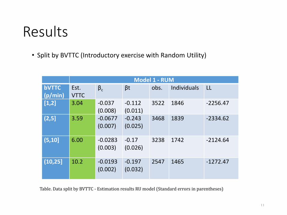
• Split by BVTTC (Introductory exercise with Random Utility)

11

Table. Data split by BVTTC - Estimation results RU model (Standard errors in parentheses)

Model 1 - RUMbVTTC (p/min)

Est. VTTC

βc βt obs. Individuals LL

[1,2] 3.04 -0.037 (0.008)

-0.112 (0.011)

3522 1846 -2256.47

(2,5] 3.59 -0.0677 (0.007)

-0.243 (0.025)

3468 1839 -2334.62

(5,10] 6.00 -0.0283 (0.003)

-0.17 (0.026)

3238 1742 -2124.64

(10,25] 10.2 -0.0193 (0.002)

-0.197 (0.032)

2547 1465 -1272.47

RV model + Random heterogeneity

BVTTC

range

Est. VTTC

p/minβwtp βwta βel βeg βI βBC βBT β∆T β∆C μ σ obs Indiv. LL

[1,2] 4.29 0.403 (0.17) 2.75 (0.58) 1.11 (0.24) 1.44 (0.36) 0.502 (0.14) 0.274 (0.1) -0.236 (0.15) 0.704 (0.3) - 0.743 (0.17) -0.248 (0.38)* 3452 1846 -2049.9

(2,5] 4.77 1.2 (0.06) 2.08 (0.17) 1.35 (0.04) 1.57 (0.09) 0.231 (0.06) 0.299 (0.08) -0.239 (0.09) 0.284 (0.15) - 1.72 (0.4) 0.16 (0.24)* 3468 1839 -2025.6

(5,10] 4.73 0.818 (0.34) 2.51 (0.13) 1.19 (0.23) 1.68 (0.09) 0.291 (0.09) 0.311 (0.1) -0.317 (0.13) 0.336 (0.21)* - 1.14 (0.3) 0.0884 (0.27)* 3238 1742 -1875.5

(10,25] 41.8 -0.522 (1.14)* 1.97 (0.35) 0.0932 (0.98)* 1.58 (0.47) 0.475 (0.2) 0.586 (0.25) -0.473 (0.27) 0.334 (0.35)* - 3.36 (1.32) 2.43 (0.87) 2547 1465 -944.7

ALL data 6.93 0.276 (0.08) 2.29 (0.07) 0.763 (0.07) 1.29 (0.06) 0.452 (0.05) 0.429 (0.06) -0.417 (0.08) 0.664 (0.07) - 1.03 (0.04) 1.25 (0.06) 12705 1874 -6856.1

ALL data 6.05 0.985 (0.06) 2.2 (0.04) 1.28 (0.04) 1.6 (0.04) 0.272 (0.03) 0.258 (0.04) -0.251 (0.05) - 0.399 (0.02) 1.72 (0.08) 0.753 (0.04) 12705 1874 -6856.1

RV model (β∆C = 0)

[1,2] 2.91 0.0431 (0.14) 2.39 (0.45) 0.747 (0.14) 1.09 (0.22) 0.502 (0.14) 0.274 (0.1) -0.235 (0.15) 0.703 (0.3) - 0.737 (0.38) - 3452 1846 -2049.9

(2,5] 4.25 1.1 (0.09) 1.98 (0.12) 1.24 (0.07) 1.47 (0.06) 0.232 (0.06) 0.3 (0.08) -0.24 (0.09) 0.284 (0.15) - 1.69 (0.38) - 3468 1839 -2025.6

(5,10] 3.98 0.65 (0.43)* 2.34 (0.07) 1.03 (0.32) 1.51 (0.15) 0.291 (0.09) 0.311 (0.1) -0.317 (0.13) 0.336 (0.21)* - 1.14 (0.3) - 3238 1742 -1875.5

(10,25] 2.84 -0.567 (1.11)* 2.05 (0.4) 0.428 (1.01)* 1.75 (0.49) 0.531 (0.23) 0.535 (0.24) -0.401 (0.28)* 0.424 (0.42)* - 0.806 (0.3) - 2547 1465 -959.4

ALL data 3.18 0.264 (0.08) 2.3 (0.07) 0.766 (0.07) 1.3 (0.06) 0.466 (0.05) 0.426 (0.06) -0.422 (0.08) 0.695 (0.07) - 0.795 (0.02) - 12705 1874 -6963.7

RV model (β∆T = 0)

[1,2] 1.81 0.873 (0.19) 2.25 (0.23) 1.29 (0.18) 1.49 (0.22) 0.295 (0.05) 0.161 (0.05) -0.138 (0.08) - 0.413 (0.1) 1.26 (0.12) - 3452 1846 -2049.9

(2,5] 4.85 1.31 (0.05) 1.99 (0.1) 1.42 (0.04) 1.6 (0.07) 0.18 (0.03) 0.233 (0.04) -0.186 (0.05) - 0.221 (0.09) 2.17 (0.27) - 3468 1839 -2025.6

(5,10] 4.71 1 (0.2) 2.27 (0.06) 1.29 (0.14) 1.64 (0.08) 0.218 (0.05) 0.233 (0.06) -0.237 (0.07) - 0.252 (0.12) 1.52 (0.22) - 3238 1742 -1875.5

(10,25] 3.83 0.572 (0.45)* 2.05 (0.28) 0.912 (0.43) 1.84 (0.29) 0.373 (0.11) 0.375 (0.14) -0.282 (0.14) - 0.298 (0.21)* 1.15 (0.2) - 2547 1465 -959.4

ALL data 4.59 0.998 (0.06) 2.2 (0.4) 1.29 (0.04) 1.61 (0.04) 0.275 (0.03) 0.251 (0.04) -0.249 (0.05) - 0.41 (0.03) 1.35 (0.06) - 12705 1874 -6963.7

* Not significant at the 90% level of confidence

• Data split by BVTTC (3 exercises with Random Valuation model)

• Data split by ∆t & Data split by ∆c

RV model (β∆T = 0, β∆C = 0)

∆t

Est.

VTTC

p/min

βwtp βwta βel βeg βI βBC βBT β∆T μ obs Indiv. LL

3 1 -0.597 (0.405) - - 0.602 (0.205) 0.519 (0.145) 0.488 (0.142) -0.231 (0.19)* - 0.65 (0.09) 2141 1100 -1067.9

5 2.89 0.285 (0.145) 2.13 (0.107) 0.487 (0.132) 1.34 (0.108) 0.389 (0.074) 0.365 (0.079) -0.265 (0.104) - 0.841 (0.05) 4485 1369 -2102.8

10 3.45 0.181 (0.125) 2.26 (0.088) 0.963 (0.084) 1.55 (0.103) 0.505 (0.071) 0.395 (0.085) -0.446 (0.11) - 0.834 (0.042) 4343 1565 -2440.6

15 4.89 0.0451 (0.51) 3.26 (0.34) 1.37 (0.16) 1.67 (0.21) 0.437 (0.15) 0.37 (0.2) -0.534 (0.24) - 0.967 (0.15) 684 298 -348.99

20 7.6 1.58 (0.27) 3.12 (0.29) 1.51 (0.25) 1.9 (0.32) 0.493 (0.17) 1.38 (0.3) -1.38 (0.39) - 0.766 (0.1) 1051 286 -628.88

ALL data 3.45 0.288 (0.08) 2.43 (0.07) 0.99 (0.06) 1.24 (0.06) 0.448 (0.05) 0.454 (0.06) -0.22 (0.07) - 0.827 (0.02) 12705 1874 -7034.3

RV model (β∆C = 0)

∆c range

Est.

VTTC

p/min

βwtp βwta βel βeg βI βBC βBT β∆T μ obs Indiv. LL

(5-15] 2.89 0.054 (0.16) 2.36 (0.46) 0.721 (0.16) 1.12 (0.33) 0.46 (0.13) 0.246 (0.1) -0.2 (0.14)* 0.748 (0.36) 0.722 (0.15) 3593 1523 -1989.3

(16-35] 3.82 0.544 (0.23) 2.44 (0.42) 0.986 (0.14) 1.39 (0.11) 0.556 (0.16) 0.562 (0.2) -0.478 (0.16) 0.558 (0.48)* 0.713 (0.21) 3455 1773 -2102.8

(35-75] 4.85 1.06 (0.26) 2.32 (0.12) 1.24 (0.19) 1.7 (0.12) 0.298 (0.09) 0.35 (0.11) -0.338 (0.1) 0.252 (0.27)* 1.29 (0.31) 2972 1586 -1552.1

(75-300] 2.3 -0.44 (0.63) 2.11 (0.19) 0.303 (0.5) 1..37 (0.28) 0.469 (0.14) 0.669 (0.19) -0.755 (0.22) 0.825 (0.35) 0.774 (0.14) 2685 1214 -1278.2

ALL data 3.18 0.264 (0.08) 2.3 (0.07) 0.766 (0.07) 1.3 (0.06) 0.466 (0.05) 0.426 (0.06) -0.422 (0.08) 0.695 (0.07) 0.795 (0.02) 12705 1874 -6963.7

* Not significant at the 90% level of confidence

Results

• What we observed splitting the data by BVTTC• VTTC = f(BVTTC)? X But… When BVTTC is closer to the underlying VTTC, precision increases.

14

• SC design settings influence model estimation of the Set of VTTC.

• Random heterogeneity: to capture the distribution, a wide range of BVTTC is needed.

• CovariatesIncome: stable effect

Current levels of Time & Cost: counteract each other (no journey length effect)

• What we observed splitting the data by ∆T & ∆C• VTTC = f(∆T)? YES Positive impact.

• VTTC = f(∆C)? Unclear

∆T & ∆C: Their role as explanatory variables vary! (i.e. VTTC = f(∆T, ∆C) not stable)

• Modelling issues: in a RV model, only one can be included as a covariate. Not obvious choice:

• Different mean VTTC

• Wider set of VTTC if ∆T is used as covariate.

Results

15

• SC design settings influence model estimation of the value of travel time.

By focussing the survey on specific settings, our sample level results will be affected…

…But some questions are left open.

• What are the roles of ∆C and ∆T? How should we model them?

• How would these results affect the way we design SC experiments?

• To what extent ∆T and ∆C effects are part of true preferences?

• Trade-off between wide BVTTC range VS focusing on the expected mean VTTC?

Thanks

16

Manuel Ojeda Cabral

Research Fellow