statecomplexesformetamorphicrobots ...ghrist/preprints/ijrr.pdfstatecomplexesformetamorphicrobots⁄...

STATE COMPLEXES FOR METAMORPHIC ROBOTS∗

A. ABRAMS† AND R. GHRIST‡

Abstract. A metamorphic robotic system is an aggregate of homogeneous robot units which canindividually and selectively locomote in such a way as to change the global shape of the system. Weintroduce a mathematical framework for defining and analyzing general metamorphic robots. With thisformal structure, combined with ideas from geometric group theory, we define a new type of configurationspace for metamorphic robots — the state complex — which is especially adapted to parallelization.We present an algorithm for optimizing an input reconfiguration sequence with respect to elapsed time.A universal geometric property of state complexes — non-positive curvature — is the key to provingconvergence to the globally time-optimal solution obtainable from the initial path.

1. Introduction. In recent years, several groups in the robotics community havebeen modeling and building reconfigurable or, more specifically,metamorphic robots

(e.g., [7, 8, 15, 17, 19, 23, 27, 28]). Such a system consists of multiple identical roboticcells in an underlying lattice structure which can disconnect/reconnect with adjacentneighbors, and slide, pivot, or otherwise locomote to neighboring lattice points followingprescribed rules: see Fig. 1.1. There are as many models for such robots as there areresearchers in the sub-field: 2-d and 3-d lattices; hexagonal, square, and dodecahedralcells; pivoting or sliding motion: see, e.g., [8, 15, 16, 17, 18, 6, 20, 27, 28] and the refer-ences therein. The common feature of these robots is an aggregate of lattice-based cellshaving prescribed local transitions from one shape to another.

Fig. 1.1. Metamorphic systems may be built on a variety of lattice structures with sliding orpivoting motion.

The primary challenge for such systems is shape-planning: how to move from oneshape to another via legal moves. One centralized approach [9, 10, 22] is to build atransition graph whose vertices are the various shapes and whose edges are elementarylegal moves from one shape to the next. It is easily demonstrated that the size of thisgraph is exponential in the number of cells.

This paper extends the notion of a configuration space to metamorphic robots in a novelmanner. The idea: consider the transition graph described above as a one-dimensionalskeleton of a higher-dimensional cubical complex, the state complex. Assume thatfrom a given state there are two legal moves which are physically independent (or, moresuggestively, “commutative”): i.e., these moves can be executed simultaneously. In

∗AA SUPPORTED BY NATIONAL SCIENCE FOUNDATION GRANT DMS-0089927. RG SUP-PORTED BY NATIONAL SCIENCE FOUNDATION GRANT DMS-0134408.

† Department of Mathematics, University of Georgia, Athens, GA 30602, USA‡ Department of Mathematics, University of Illinois, Urbana, IL 61801, USA

1

2 AARON ABRAMS & ROBERT GHRIST

the transition graph, this corresponds to the four edges of a square. For any pair ofcommutative moves, fill in the four edges of the graph with an abstract square 2-cell.Continue inductively adding k-dimensional cubes corresponding to k-tuples of physicallyindependent motions. The result is a cubical complex which has several advantages overthe transition graph:

1. Simplicity. The state complex, though larger than the (already large) tran-sition graph, is often topologically much simpler: e.g., the 1-d graph of ann-dimensional cube has n2n−1 edges. The number of edges is not necessarily thebest measure of complexity: it belies the simplicity of the single cube.

2. Speed. Geodesics on this complex cut across the diagonals of cubes wheneverpossible. One performs all possible commutative motions simultaneously, maxi-mizing parallelization and yielding a speed-up by a factor equal to the numberof coordinated motions.

3. Shape. The global geometry/topology of the state complex carries informa-tion about the metamorphic system. For certain examples, the topology of thestate complex “converges” upon refining the lattice. In addition, only specialgeometries can be realized as the state complex of a local metamorphic system:commutativity in reconfiguration leads to an abhorrence of positive curvature inthe state complex.

Sections 2 through 4 give definitions and examples of [abstract] metamorphic systemsand their state complexes. The next two sections (Sections 5-6) detail topological andgeometric features of the state complex.

For large systems, the problem of computing the state complex and designing geodesics inorder to perform shape planning is computationally infeasible, primarily because the sizeof the complex is often exponential in the number of robot cells. In addition, any controlscheme induced by geodesic construction is necessarily centralized. Several researchershave begun building decentralized control algorithms for shape planning [5, 25, 24, 26,29, 30]. Such algorithms have the advantage of speed and scalability; however, thereconfiguration paths are typically not optimal.

We present an algorithm which works in conjunction with these fast planners to optimizetheir paths. In Sections 7-8, we present an algorithm for trajectory optimization whichtakes as its argument an arbitrary edge path in the transition graph. Algorithm 8.2then performs a type of curve shortening within the state complex. A deep theoremabout the curvature of all state complexes (Theorem 6.2) is then used to prove that thisalgorithm returns a shape trajectory which is the global minimum obtainable from thispath with respect to elapsed time.

Our definitions and theorems are phrased for systems involving “discrete” reconfigura-tion. More general types of robots which employ continuous reconfiguration for locomo-tive gaits (such as the Polybot developed by M. Yim’s lab at PARC) are not coveredby our definitions. We note, however, that certain locomotive reconfigurable robots canbe thought of as lattice-based tiles by amalgamating subsystems [16]. In addition, ourdefinitions can easily be extended to more general non-lattice reconfigurable systems [3].

2. A mathematical definition. While it is easy to generate examples of what ismeant by a metamorphic robot, it is more challenging to write a clean mathematicaldefinition. We propose a set of definitions which is broad enough to include some non-

STATE COMPLEXES 3

obvious examples. The paper [6] suggests a similar type of structure using cellularautomata rule sets.

A local metamorphic system is a collection of states on a lattice (or, more generally, agraph), where each state is thought of as a labeling function for the aggregate. In mostexamples, the alphabet of labels will be {0, 1} and will be used to denote the absence orpresence (resp.) of a module at that lattice point. Any state can be modified by localrearrangements, these local changes being coordinated by a catalogue of models realizedunder the actions of isometries into the workspace. The adjective “local” refers to legalitycriteria: anywhere in the workspace at which a local change from the catalogue can beapplied, it is legal to do so. To incorporate obstacles and basepoints into our systems,we distinguish between the amount of information needed to determine the legality ofan elementary move (the “support” of the move) and the precise place in which modulesare actually in motion (the “trace” of the move).

Definition 2.1. Let L denote a lattice in Rk, let W ⊂ L denote a compact workspace,and let A denote an alphabet of labels. The catalogue C for a local metamorphic systemon W is a collection of generators. Each generator φ ∈ C consists of (1) the support,sup(φ) ⊂ L; (2) the trace of the move, tr(φ) ⊂ sup(φ); and (3) an unordered pair oflocal states U0,1 : sup(φ)→ A satisfying1

U0

∣

∣

∣

sup(φ)−tr(φ)= U1

∣

∣

∣

sup(φ)−tr(φ).(2.1)

Otherwise said, the local states are equal on sup(φ)− tr(φ).

Definition 2.2. An action of a generator φ ∈ C is a rigid translation Φ : sup(φ) ↪→W. Given a state U :W → A, an action Φ is said to be admissible at U if U0 = U ◦Φ.In this case, we write

φ[U ] :=

{

U : on W −Φ(sup(φ))

U1 ◦Φ−1 : on Φ(sup(φ))

.

(Note that Φ is left out of the notation.)

Definition 2.3. A local metamorphic system on W is a collection of states{Uα :W → A} closed under all possible admissible actions of generators in the catalogueC.

To repeat, the catalogue and the workspace are the “seeds” for a local metamorphicsystem. From this pair, all possible translations of the supports intoW yield the actions.Then, a collection of states on the workspace is a local metamorphic system if, wheneveran action Φ of a generator φ on a state U is admissible, then the corresponding stateφ[U ] is also included.

A metamorphic system with obstacles O ⊂ W satisfies in addition

Φ(tr(φ)) ∩ O = ∅,(2.2)

for each φ ∈ C. Obstacle sets count as legal positions for determining the admissibilityof a move (the support of an action may intersect O), but no motion of metamorphicagents may incorporate the obstacle sites (the trace of an action must not intersect O).

1All generators are assumed to be nondegenerate in the sense that U0 6= U1.


3. Examples. Some of the following examples are inspired by metamorphic robotsalready developed; other examples are more abstract. Unless otherwise noted, the al-phabet A is {0, 1}, denoting unoccupied or occupied cells.

Example 3.1. [2-d hex with pivots] We present two slightly different catalogues, eachwith six generators (or one, up to discrete rotations), in Fig. 3.1. Both of these systems,modeled after that of [8], have local moves which pivot a planar hexagon about a neigh-bor. For all generators presented, the trace is equal to the two central hexagons. In thefirst system, the support is chosen so that the aggregate does not change its topologybut only its shape. The slightly smaller support of the second catalogue allows for localtopology changes. To model a fixed “base” cell (which is, say, affixed to a power sourceas in [20]), one establishes this cell as an obstacle O.

Fig. 3.1. Two different catalogues for a 2-d hexagonal lattice system with pivots. Black cells areoccupied, white are unoccupied. The local states U0 and U1 are shown for each generator.

Example 3.2. [2-d square lattice] In Fig. 3.2, we display a generator for a planarsystem in which rows [as pictured] and columns [not pictured] of an aggregate of squarecells can slide. There are in fact several generators represented in “shorthand,” one foreach k ≥ 0. A dot inside a cell indicates that it can be either occupied or unoccupied,but if occupied, then its neighbor (indicated by an arrow) must also be occupied. Thiscondition guarantees that the aggregate does not disconnect (even locally) under slides.The trace of this set of generators is the entire middle row except the two endpoints. Tokeep the catalogue finite, one would include only those generators with k ≤ N , where Nis the number of occupied cells in any state.

PSfrag replacements

kk

01

Fig. 3.2. The row-sliding generators for a sliding-squares system.

Example 3.3. [2-d articulated planar arm] Consider as a workspace W the set ofedges in the planar integer lattice. The catalogue consists of two generators, pictured inFig. 3.3. Beginning with a state having N vertical edges end-to-end, the metamorphicsystem thus generated models the position of an articulated robotic arm with fixed basewhich can (1) rotate at the top end and (2) flip corners as per the diagram.

If one includes rotations of these generators, more intricate types of configurations arepossible, including deadlocked configurations. Examples with multiple interacting armscan be realized by adding new generators: an “attach-detach” generator which allowsendpoints of arms to merge (thus yielding a “marked point” at the attachment); and a“sliding” generator which allows this marked point to slide, having the effect of allowing

STATE COMPLEXES 5

Fig. 3.3. A positive articulated robot arm [left]. One generator [center] flips corners and has asits trace the central four edges. The other generator [right] rotates the end of the arm, and has traceequal to the two activated edges.

the attached arms to trade segments. These generators are pictured (up to Euclideansymmetries) in Fig. 3.4.

Fig. 3.4. Additional generators allow for attachment and detachment of arm endpoints [left, center]and sliding of the coupling points [right].

Example 3.4. [2-d expansion-compression square system] Consider a planar squarelattice workspace. This system will use an alphabet of labels A = {0, 1,=, ‖} whoseinterpretation is as follows: “0” means that a cell is unoccupied; “1” means that the cellis occupied by one module; “=” and “‖” imply that the cell is occupied by two modulescompressed together in a horizontal or vertical orientation (resp.). The catalogue consistsof six generators, illustrated in Fig. 3.5 (the lower two generators are only representedup to flips). The trace is equal to the support for the top two generators illustrated;for the bottom two generators, the trace is equal to the support minus the single squarewhich remains unoccupied (label “0”).

This example is a local system based on the Crystalline robots of Rus et al. [23]. Ex-tensions to 3-d cubical systems and more elaborate motions can be accommodated withminor modifications.

One of the benefits of writing down a rigorous definition of a metamorphic system is thediscovery of systems which have little resemblance to the systems of, say, Fig. 1.1. Inparticular, our definitions easily extend to metamorphic systems which are not lattice-based. The following example is especially interesting.

Example 3.5. Consider a finite graph Γ in which every edge is assigned a length ofone. (Every graph can be embedded in some Rk so as to have this property.) Thecatalogue consists of a single generator whose support and trace are precisely the closureof a single abstract edge. The local states of this generator consist of the pair U0 andU1 which evaluate to 1 on one of the endpoints and 0 on the other. The actions in thiscase are length-preserving maps from the abstract edge into Γ. The metamorphic system


Fig. 3.5. Generators for a simple compression-expansion system on the square planar lattice [left];an example of a typical state [right].

generated from a state U on Γ with N vertices evaluating to 1 mimics an ensemble of Nunlabeled non-colliding Automated Guided Vehicles on Γ, cf. [13]. To work with labeledvehicles, one need merely increase the alphabet A to accommodate the different labels.

More abstract examples of metamorphic examples include spaces of triangulations ofpolygons with edge-flipping as the generator, examples arising from word representationsin group theory, and certain multi-step assembly processes [3].

4. The state complex. In the robotics literature, one often models a configurationspace for a metamorphic system with a transition graph which represents actions ofelementary moves on states. That is, the vertex set is the collection of all states {Uα},and the edges are unoriented pairs of states which differ by the action of one generator.Transition graphs are discussed for shape-planning in several particular cases in theliterature (planar hex case: [9, 22]). Our departure is to make the transition graph the1-skeleton of a cubical complex (an analogue of a simplicial complex, but made out ofabstract cubes) which coordinates parallel or “commutative” motions.

Definition 4.1. In a local metamorphic system, a collection of actions of (not neces-sarily distinct) generators {(φαi

,Φαi)} is said to commute if

Φαi(tr(φαi

)) ∩Φαj(sup(φαj

)) = ∅ ∀i 6= j.(4.1)

Example 4.2. Two simple examples suffice to illustrate the difference between com-muting and noncommuting actions. First, consider the pair of commuting moves for aplanar hexagonal pivoting system, as represented in Fig. 4.1 [left]. Compare this with aplanar sliding block example as illustrated in Fig. 4.1 [right]. Although the pair of movesillustrated forms a square2 in the transition graph, this particular pair of actions doesnot commute. Physically, it is obvious why these moves are not independent: sliding thecolumn part-way obstructs sliding a transverse row. Mathematically, this is captured bythe traces of the actions intersecting.

The state complex has an abstract k-cube for each collection of k admissible commutingactions:

2The individual robotic cells are not labeled: only the shape of the aggregate is recorded.

STATE COMPLEXES 7

Fig. 4.1. Examples of commuting [left] and noncommuting [right] actions in planar systems.

Definition 4.3. The state complex S of a local metamorphic system is the fol-lowing abstract cubical complex. Each abstract k-cube e(k) of S is an equivalence class[U ; (Φαi

)ki=1] where

1. (Φαi)ki=1 is a k-tuple of commuting actions of generators φαi

;2. U is some state for which all the actions (Φαi

)ki=1 are admissible; and3. [U0; (Φαi

)ki=1] = [U1; (Φβi)ki=1] if and only if the list (βi) is a permutation of

(αi) and U0 = U1 on the set W −⋃

iΦαi(sup(φαi

)) .

The boundary of each abstract k-cube is the collection of 2k faces obtained by deletingthe ith action from the list and using U and φαi

[U ] as the ambient states. Specifically,

∂[U ; (Φαi)ki=1] =

k⋃

i=1

(

[U ; (Φαj)j 6=i] ∪ [φαi

[U ]; (Φαj)j 6=i]

)

.(4.2)

It follows easily that the k-cells are well-defined with respect to admissibility of actions.The proof of the following obvious lemma is given in detail to flesh out the previousdefinition.

Lemma 4.4. (a) The 0-dimensional skeleton of S, S (0), is the set of states in the recon-figurable system. (b) The 1-dimensional skeleton of S, S (1), is precisely the transitiongraph.

proof: (a) Vertices of S consist of equivalence classes consisting of zero (i.e., no)actions of generators up to permutation, together with a state defined on the complementof the supports of the actions. As there are no actions, each 0-cell is precisely a singlestate of the reconfigurable system.

(b) A 1-cell of S is an equivalence class of the form [U ; (Φ)]. The only other representativeof the equivalence class is [φ[U ]; (Φ)]; hence, the 1-cells are precisely the edges in thetransition graph. Clearly, the boundary of [U ; (Φ)] is the pair of 0-cells [U ; (·)] and[φ[U ]; (·)]. ¦

For small numbers of cells, it is easy to illustrate the state complex.

Example 4.5. Consider the 2-d square lattice row/column sliding system whose cata-logue is illustrated in Fig. 3.2. If we consider a system with fixed obstacles in the form of


PSfrag replacements

p

q

Fig. 4.2. The planar sliding square example [left] with two movable blocks [in grey] and a p-by-qobstacle set [in black] yields a state complex S that is topologically a circle [right]. Sample configurationsin the state complex are illustrated.

a p-by-q rectangle generated from the state of Fig. 4.2 [left], one obtains a planar transi-tion graph with 4(pq+1)+ 2(p+ q) vertices and 8(pq+1)− 2(p+ q) edges. In contrast,the state complex is that of Fig. 4.2 [right]: this is topologically a circle, correspondingto the fact that the pair of free squares can circulate about the obstacle set througha sequence of slides. The large 2-d regions correspond to states in which the two freesquares are on separate (but adjacent) sides of the obstacle set.

Example 4.6. Consider the planar hex system of Fig. 3.1 [left] with a workspace Wconsisting of a long channel of four rows with a line of occupied cells attached to a fixedobstacle at the right. This line of cells can “climb” on itself from the left and migrate tothe right, one by one. The entire state complex is illustrated in Fig. 4.3[right]. Althoughthe transition graphs appear complicated, this state complex is contractible for anylength channel.

Fig. 4.3. For a line of hexagons filing out of a constrained tunnel [left], the state complex iscontractible [right]. Black cells represent obstacle sets. A short tunnel is shown: for longer tunnels, thestate complex has higher dimension, but is still contractible.

Example 4.7. The state complex associated to the positive articulated robot arm ofExample 3.3 in the case N = 5 is given in Fig. 4.4. Note that there can be at most threeindependent motions (when the arm is in a “staircase” configuration); hence the statecomplex has top dimension three. Notice also that although the transition graph for thissystem is complicated, the state complex itself is topologically trivial (contractible).

Example 4.8. In the system of Example 3.5 with the graph being a K5 (the completegraph on five vertices) and N = 2, the state complex is a two-dimensional closed surface.A simple combinatorial argument (as in [1, 2]) reveals that the Euler characteristic is−5, implying that the state complex is non-orientable. If the AGV’s are labeled, thestate complex becomes a closed orientable surface of genus 6.

STATE COMPLEXES 9

Fig. 4.4. The state complex of a 5-link positive arm has one cell of dimension three, along withseveral cells of lower dimension.

5. The topology of S. If one looks at a transition graph without knowing theparticulars of the metamorphic system, very little information can be extracted. Thispaper argues that completing the transition graph to the state complex is “natural” —the state complex simplifies the transition graph and endows it with topological andgeometric content.

Our first example of naturality is motivated by the desire to build metamorphic systemswith large numbers of micro- or nano-scale cells. While large numbers of cells would yielda type of continuum-limit convergence on the dynamics of shape change, the resultingtransition graphs have no such convergence. The size of the transition graph goes upexponentially in the number of cells; more ominous is that the topology of the transitiongraph (the number of basic cycles) blows up as well. This is not always so with the statecomplex: in certain key examples, the topology of S is either invariant or converges to alimiting type.

We have already seen one such example of this stabilization. In Example 4.5, the statecomplex of a pair of squares sliding along a rectangular obstacle of size p-by-q is topolog-ically a circle, independent of p and q. This can be interpreted as a type of convergence:consider the effect of refining the underlying lattice structure, increasing p and q whilemaintaining a pair of sliding squares. Then the dimension of the state complex remainsthe same, as does the topological type of the space. Intuitively speaking, the “limit” asthis refining process is repeated yields a “topological” configuration space of two pointssliding smoothly along the boundary of a rectangle, which can dock or un-dock at thecorners.

Example 5.1. Recall the state complex associated to the metamorphic system of Npoints on a graph Γ, Example 3.5. Consider a refinement of Γ which inserts additionalvertices along edges. It follows from the techniques of [1] that the state complex ofthis refined system has the same topological type (up to homotopy equivalence) aftera fixed bound on the refinement (N additional vertices per edge). Furthermore, this“stabilized” state complex is in fact homotopic to the topological configuration space ofN non-colliding points of Γ — precisely what one expects as the number of refinementsgoes to infinity.

Example 5.2. Recall the positive articulated robot arm of Example 3.3. Consider arefinement of the underlying lattice which shrinks the lattice by a factor of two (or,equivalently, which inserts an additional joint in the middle of each edge). This is amore dramatic change since the dimension of the state complex doubles. Nevertheless,the topological type is invariant: the state complex remains contractible.

Proposition 5.3. Let SN denote the state complex of the positive articulated arm from


Example 3.3 with N segments. The complexes SN are all contractible.

proof: For these articulated arms, there is a nice inductive structure on the statecomplexes. Fixing N , each state (vertex) in SN is represented as a length N word inthe symbols x and y, where x denotes the arm going to the right and y denotes the armgoing up. In this language, the two generators are (1) transposing a subword xy ↔ yx,and (2) changing the last letter of the word.

Consider the subcomplex X ⊂ SN consisting of all cells whose vertices have wordsbeginning with the letter x. Likewise, let Y denote the subcomplex all of whose verticesbegin with the letter y. These subcomplexes are each a copy of SN−1 which we mayassume inductively is contractible. One passes between the subcomplexes X and Y onlywhen a move exchanges the initial two letters of the word from xy to yx. The connectingset is thus homeomorphic to SN−2 × [0, 1] and attached to X and Y along SN−2 × {0}and SN−2 × {1} respectively. Again, by induction, these sets are contractible. A pair ofcontractible sets joined along contractible subsets is contractible. ¦

This should come as no surprise: in the limit as N → ∞, the metamorphic system ap-proximates the configuration space of a smooth curve of fixed length which is positivein the sense that the curve is always nondecreasing in the horizontal and vertical com-ponents. That the (infinite dimensional) space of such smooth curves is contractible iseasily demonstrated: given any such curve with endpoint fixed at the origin in the plane,pull the other end along the straight line connecting it to the origin until the strand istaut. Then, rotate the line segment rigidly until it is, say, vertical. This is a continuousdeformation on the space of all smooth positive curves of fixed length to a single verticalsegment.

It is certainly not the case that an arbitrary reconfigurable system possesses such con-vergence properties: the manner in which one refines the states is important. Still, itappears that state complexes can often be viewed as “discretizations” of some underlyingsmooth configuration space. This is an important focus for future inquiry.

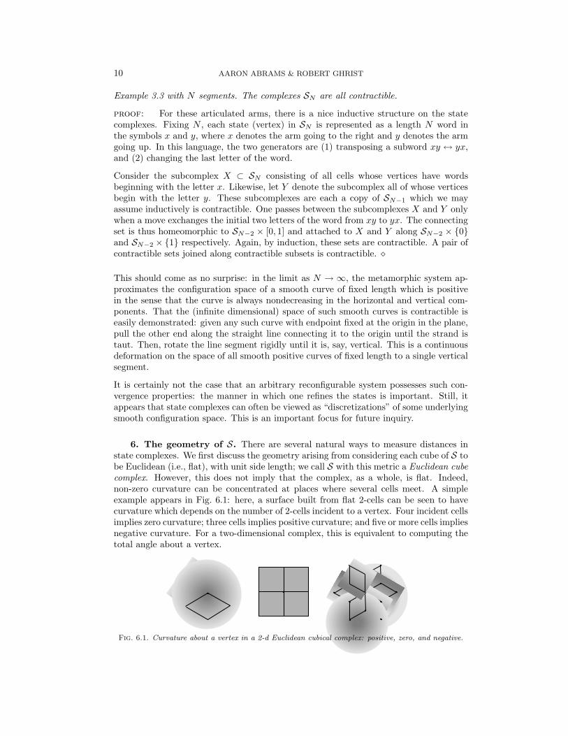
6. The geometry of S. There are several natural ways to measure distances instate complexes. We first discuss the geometry arising from considering each cube of S tobe Euclidean (i.e., flat), with unit side length; we call S with this metric a Euclidean cubecomplex. However, this does not imply that the complex, as a whole, is flat. Indeed,non-zero curvature can be concentrated at places where several cells meet. A simpleexample appears in Fig. 6.1: here, a surface built from flat 2-cells can be seen to havecurvature which depends on the number of 2-cells incident to a vertex. Four incident cellsimplies zero curvature; three cells implies positive curvature; and five or more cells impliesnegative curvature. For a two-dimensional complex, this is equivalent to computing thetotal angle about a vertex.

Fig. 6.1. Curvature about a vertex in a 2-d Euclidean cubical complex: positive, zero, and negative.

STATE COMPLEXES 11

Such an extension of curvature to general metric spaces is made precise in Gromov’s workon curved metric spaces [14] (extending the classical work of Alexandrov, Busemann, andothers) in which triangles with geodesic edges are used to measure curvature bounds. Inbrief, let X be a metric space and p ∈ X a point. To bound the curvature of X at p,consider a small triangle T about p with geodesic edges of length a, b, and c. Build acomparison triangle T ′ in the Euclidean plane whose sides also have length a, b, andc respectively. Choose a geodesic chord of T and measure its length d. In T ′, measurethe length d′ of the chord whose endpoints correspond to those of the chord in X.

Definition 6.1. A metric space X is nonpositively curved (or NPC) if for everysufficiently small geodesic triangle T and for every chord of T , it follows that d ≤ d′.

PSfrag replacements

ab

c

d

a b

c

d′

X R2

Fig. 6.2. Comparison triangles measure curvature bounds.

In other words, geodesic chords are no longer than Euclidean comparison chords. Itshould be stressed that the NPC property is very special and highly desirable. Indeed,being NPC implies a variety of topological consequences reminiscent of smooth nonpos-itively curved manifolds.

Despite the variety of (local) metamorphic systems, all state complexes share this specialgeometric property.

Theorem 6.2. The state complex S of any local metamorphic system is nonpositivelycurved.

The proof of this theorem is simple, but requires some additional machinery.

Definition 6.3. Let X denote a complex (either simplicial or cubical) and let v denotea vertex of X. The link of v, `k[v], is defined to be the abstract complex which hasone k-dimensional simplex for each (k + 1)-dimensional cube in X incident to v. Theboundary relations are those inherited from X: namely, the boundary of a k-simplex in`k[v] represented by a (k + 1)-cube in X is the set of all simplices represented by thefaces of the (k + 1)-cube.

Links can be thought of as a simplicial version of the locus of points a small fixed distancefrom the vertex v.

Definition 6.4. A Euclidean cube complex X satisfies the link condition if, for eachvertex v ∈ X, `k[v] satisfies the following: for each k, if any k + 1 vertices in `k[v] arepairwise connected by edges in `k[v], then those vertices bound a unique k-simplex in`k[v].

An important and deep theorem of Gromov [14] asserts that a Euclidean cube complexis nonpositively curved if and only if it satisfies the link condition. This criterion makesit easy to prove Theorem 6.2.


proof of theorem 6.2: Let U denote a vertex of S. Consider the link `k[U ]. The 0-cells of the `k[U ] correspond to all edges in S incident to U ; that is, actions of generatorsadmissible at the state U . A k-cell of `k[U ] is thus a commuting set of k + 1 of theseactions based at U . The interpretation of the link condition for a state complex is asfollows: if at U one has a set of k + 1 admissible actions, {(φαi

,Φαi)}k+1i=1 , of which

each pair commutes, then the full set of k+1 generators must commute [existence of thek-simplex in the link]. Furthermore, they must commute in a unique manner [uniquenessof the k-simplex in the link].

The proof of existence follows directly from Definition 4.1: any collection of pairwisecommutative actions is totally commutative. We therefore have a (k + 1)-dimensionalcell in S which is the equivalence class [U ; (Φαi

)k+1i=1 ]. This is the representative in S of

the k-simplex in `k[U ]. To show uniqueness, consider any other k-simplex in `k[U ] whichhas the same vertex set. This must correspond to a (k + 1)-dimensional cube in S withactions (φαi

,Φαi)k+1i=1 (up to some permutation) based at U . From Definition 4.3, this

cell must be the same equivalence class, namely [U ; (Φαi)k+1i=1 ]. ¦

Example 6.5. To see how the NPC property can fail, consider the following non-localmetamorphic system. Recall the generator for the planar hexagonal system presentedin Fig. 3.1[right] which (along with its rotations) allows for local disconnection of theaggregate. If we add to this system a global rule that requires the aggregate to beconnected (for, say, considerations of power transmission), then we no longer have alocal system, and positive curvature may exist. Fig. 6.3 shows a configuration in whichthree actions of local generators act to disconnect the aggregate locally but not globally.These actions commute pairwise, and any two do not disconnect globally. However,performing all three actions disconnects the space and leads to an illegal state. Therefore,the corresponding state complex for this non-local system has a “corner” of positivecurvature as a local factor. Note: the state complex will not be two-dimensional here,but will be locally a product of this with another cubical complex. The positive curvaturepersists.

Fig. 6.3. A generator which allows for local disconnection [left] admits configurations [center]for which pairs of actions leave the aggregate connected, but triples do not; this non-local system haspositive curvature in the state complex at this vertex [right].

7. Geodesics and time on S. Besides displaying a unifying geometric feature, thenonpositive curvature has implications for path-planning, and, hence, the shape-planningproblem.

Corollary 7.1. Each homotopy class of paths connecting two given points of a statecomplex contains a unique shortest path.

STATE COMPLEXES 13

proof: This is well-known for NPC spaces. The only difficulty lies in proving thatthe d ≤ d′ inequality for sufficiently small triangles implies the d ≤ d′ inequality for allgeodesic triangles which are contractible in the space: see [4]. Assume, then, that thisinequality holds in general, and consider a pair of distinct homotopic shortest paths frompoints p to q in S. Choose any point r on one of the two paths. The two halves of thispath bisected by r are themselves shortest paths from p to r and r to q respectively.Thus, there is a geodesic triangle in S whose comparison triangle in the Euclidean planeis a degenerate straight line from p′ to q′. The d ≤ d′ inequality applied to the segmentfrom r to its corresponding point on the other geodesic shows that these points coincide;therefore the two shortest paths from p to q in S are identical. ¦

Fig. 7.1[left] gives a simple example of a 2-d cubical complex with positive curvature forwhich the above corollary fails.

This corollary is a key ingredient in the applications of NPC geometry to path-planningon a configuration space, since one expects geodesics on S to coincide with optimalsolutions to the shape planning problem. However, in the context of robotics applications,the goal of solving the shape-planning problem is not necessarily coincident with thegeodesic problem on the state complex. Fig. 7.2[left] illustrates the matter concisely.Consider a portion of a state complex S which is planar and two-dimensional. To getfrom point p to point q in S, any edge-path which is weakly monotone increasing in thehorizontal and vertical directions is of minimal length in the transition graph. The truegeodesic is, of course, the straight line, which is not well-positioned with respect to thediscrete cubical structure.

Fig. 7.1. [left] A 2-d cube-complex (with positive curvature) possessing two distinct homotopicshortest paths between a pair of marked points; [right] a 2-d cube-complex (with positive curvature)possessing an edge path (the thick line on the boundary) which is a locally (but not globally) shortestpath. Any cube path near this path is strictly longer. Note: for both of these complexes, all edges areassigned unit length.

Given the assumption that each elementary move can be executed at a uniform maximumrate, it is clear that the true geodesic on S is time-minimal in the sense that the elapsedtime is minimal among all paths from p to q. However, there is an envelope of non-geodesic paths which are yet time-minimizing. Indeed, the true geodesic in Fig. 7.2[left]“slows down” some of the moves unnecessarily in order to maintain the constant slope.

This leads us to define a second metric on S, one which measures elapsed time. Namely,instead of the Euclidean metric on the cells of S, consider the space S with the `∞

norm on each cell. (This is also called the supremum norm: a vector is measured bythe maximum of its components in each coordinate direction.) The geodesics in thisgeometry represent reconfiguration paths which are time minimizing. Using the resultsof [21], one can prove that these geodesics are easily described using the notion of a cube


Fig. 7.2. [left] The true geodesic lies within an envelope of time-minimizing paths. No minimaledge-paths are time-minimizing; [right] a normal cube-path in an NPC complex (after [21]).

path.

Definition 7.2. A cube path from a vertex v0 to a vertex vN is an ordered sequenceof closed cubes {Ci}

N1 in S which satisfy (1) Ci ∩ Ci+1 = vi for some vertex vi; and (2)

Ci is the smallest cell of S containing vi−1 and vi. A cube path is said to be normal ifin addition, (3) for all i, St(Ci) ∩ Ci+1 = vi, where St(Ci) is the star of Ci (the unionof all closed cubes, including Ci, which have Ci as a face).

Roughly speaking, a normal cube path is one which uses the highest dimensional cubesas early as possible in the path.

Theorem 7.3. In any state complex S, there exists a unique normal cube path from pto q in each homotopy class. The chain of diagonals through this cube path minimizestime among all paths in its homotopy class.

This result follows from Theorem 6.2 and a result of [21] (or, see the constructive algo-rithm of Section 8 below for a proof of existence).

This result also implies that, in the category of homotopic cube-paths, there is no suchthing as a strictly local minimum for length. See Fig. 7.1[right] for a simple example ofa cube complex with some positive curvature that has a cube path which is locally ofminimal length among cube paths, but not globally so.

This is very significant. Beginning with any path in the state complex, say, one obtainedvia a fast distributed algorithm for shape-planning, one can employ a gradient-descentcurve shortening on the level of cube paths. The above results imply that any algorithmwhich monotonically reduces length must converge to the shortest path (in that homo-topy class) and cannot be hung up on a locally minimal cube path. The presence oflocal minima is a persistent problem in optimization schemes: nonpositive curvature isa handy antidote.

8. Optimizing paths. In cases where the state complex is sparse — local principalcells being of high dimension with few neighbors — it is possible to compress the com-plex significantly. However, shape-planning via constructing all of S and determininggeodesics is, in general, computationally infeasible: the total size of the state complex isoften exponential in the number of cells in the aggregate. We therefore assume that someshape trajectory has been determined (perhaps by one of the many excellent decentral-ized planners available [5, 6, 24, 25, 26, 29]) and turn to the problem of optimizing thistrajectory. The nonpositive curvature of S allows for a time-optimization which does notrequire explicit construction of S. We detail an algorithm for transforming any given

STATE COMPLEXES 15

edge-path to a time-optimal normal cube path.

From Definition 4.3, an n-dimensional cube C of S can be represented by a set of ncommutative actions {Φi} along with an admissible state U . In the following algorithm,we suppress the state for notational convenience and consider C as the set of actions.Addition and subtraction is defined by adding or taking away admissible commutativeactions to the list.

Algorithm 8.1 (TimeGeodesic). Given: a cube path C = {Ci}i=1..N in S.

1: Let N := Length(C).2: Call ShrinkCubePath(C).3: If Length(C) < N then 1: else stop.

Algorithm 8.2 (ShrinkCubePath). Given: a cube path C = {Ci}i=1..N in S.

1: Let i = 1.2: Let X := Commute(Ci;Ci+1).3: Update Ci := Ci +X;

4: Update Ci+1 := Ci+1 −X.

5: Call ExciseTrivial(Ci+1).6: Call CommonEdge(Ci−1, Ci).7: Call ExciseTrivial(Ci−1;Ci).8: If X = ∅ then i = i+ 1.9: If Ci+1 6= ∅ then 2: else stop.

Subroutine 8.3 (Commute). Given: a pair of cubes Cj = {Φjαi}i=1..m and Cj+1 =

{Φj+1βi}i=1..n,

1: Let S :=⋃

i sup(Φjαi)

2: Let T :=⋃

i tr(Φjαi)

3: For i = 1..n return Φj+1βi

if

3.1: S ∩ tr(Φj+1βi

) = ∅ ; and

3.2: T ∩ sup(Φj+1βi

) = ∅.

Subroutine ExciseTrivial checks a cube for an empty list, removes these from thepath, and re-indexes the cube path, thus reducing the length. Subroutine CommonEdge

checks a cube against adjacent cubes in the sequence for common edges and deletes these,returning a genuine cube path (recall Definition 7.2).

Subroutine Commute takes as its argument a pair of cubes Ci and Ci+1 and returns thoseelements of Ci+1 which commute with all elements of Ci. The following lemma is amanipulation of the definitions.

Lemma 8.4. The result of Commute(Ci;Ci+1) is precisely the set of edges in St(Ci) ∩Ci+1.

Theorem 8.5. Given a cube path C, Algorithm 8.1 computes a globally time-optimalpath in the homotopy class of C.

proof: Recall that in this setting, the length of a cube path refers to the number ofcubes in the path; this equals the time required to execute the reconfiguration.

Repeated calls to Algorithm ShrinkCubePath eventually leave a cube path fixed. To


PSfrag replacements

C 1

2 3

Fig. 8.1. Three rounds of shortening an edge path C. Cube path length stabilizes after two calls toShrinkCubePath. Three more calls produces a normal cube path.

show this, note that the integer-valued function f(C) :=∑

i i · dim(Ci) decreases in eachcall to ShrinkCubePath which changes the path. Lemma 8.4 implies that ShrinkCubePathleaves a cube path fixed if and only if it is a normal cube path. From Theorem 7.3, thisyields a time-optimal path.

However, Algorithm TimeGeodesic calls ShrinkCubePath only until the length of thecube path is unchanged. Thus it remains to show that once the length of a cube pathin unchanged by a call to ShrinkCubePath, this is equal to the length of the associatednormal cube path. To show this, assume that ShrinkCubePath stops without excisingany trivial cubes (i.e., shortening the length). We show that further calls merely redis-tribute actions earlier in the list C without deleting any permanently. Without a lossof generality, assume that the first call to ShrinkCubePath does not change the lengthof the cube path, but that in the subsequent call, the cube Ci+1 is eliminated via Cicommuting with a portion of Ci−1: see the schematic of Fig. 8.2.

PSfrag replacements

Ci+1Ci+1

Ci−1Ci−1

Ci−1

CiCiCi =

Fig. 8.2. Schematic of exchanging actions in sequential rounds. Each dimension in this cartoonrepresents a multi-dimensional cube.

Since Ci+1 is not eliminated in the first call, there must have been actions in Ci whichdid not commute with those of Ci−1 but which are subsequently pushed backward in thesecond call. In addition, all the actions of Ci+1 are contained in (“parallel to” in thefigure) the subset of Ci−1 which commutes with Ci in the second call. This being the case,the commutativity of Ci+1 with Ci would have occurred in the first call: contradiction.¦

It is not surprising that Algorithm 8.1 converges to a locally time-minimal solution. Theinteresting implication is that the cube-path obtained is the global minimum for all pathsobtainable from the initial: there is no way to get a quicker reconfiguration path by first

STATE COMPLEXES 17

lengthening the path and then shortening. This is the boon of nonpositive curvature.

In Fig. 8.1, we illustrate the effect of Algorithm 8.1 on an initial edge-path in a (verysimple Euclidean) state complex. Here, the two types of path-improvement are displayed:(1) commutative moves are executed simultaneously, resulting in higher dimensionalcubes being utilized; (2) redundant “backtracking” is eliminated.

Example 8.6. Consider a decentralized shape-planning algorithm which takes any con-nected aggregate of planar hex cells and simplifies it (using the catalogue of Fig. 3.1[right])to a straight line by moving cells one at a time. This yields a shape-planner by com-posing a path from the initial shape to the straight line with the inverse of the pathfrom the final shape to the straight line. See Fig. 8.3[top] for a path which translatesa small “pile” of three hexes across a long fixed base of N hexes in this manner. Thistype of reconfiguration path requires precisely 3N +13 edges (or time-steps). Using thisedge-path as an input to Algorithm 8.1 yields a path of length N + 2: as illustrated inFig. 8.3[bottom], commutative motions are performed simultaneously and backtrackingis eliminated. The speed-up in elapsed time from 3N + 13 to N + 2 is, roughly, a factorof three — the “average” dimension of the state complex near the initial edge path. Thiscorresponds to the fact that most of the steps involve simultaneous motion of all threehexes.

Fig. 8.3. An example of a planar hex system reconfiguration under the action of Algorithm 8.1:[top] an unsimplified edge path; [bottom] the simplified reconfiguration path. The horizontal coordinatedenotes time. Dark hexes correspond to fixed cells.

The complexity of Algorithm 8.1 depends on both the catalogue of generators for thesystem and the length N of the input edge path. However, the dependence on thecatalogue arises only in Subroutine Commute, which tests various pairs of subsets of theworkspace for disjointness; the sizes of these subsets are governed by the generators.Assuming a fixed catalogue, then, there is a constant bound on the time required for asingle call to Commute, and we may analyze the complexity of Algorithm 8.1 as a functionof N alone.


Notice that Algorithm 8.1 calls ShrinkCubePath at most N times, since it stops assoon as the length of the cube path fails to decrease. Each time an individual loopof ShrinkCubePath is executed, the quantity

∑

dim(Cj) decreases. Since this quantityequals N initially, ShrinkCubePath calls the subroutines Commute, ExciseTrivial, andCommonEdge each at most N times. Each of these has a constant running time, withCommute being the only one depending on the particulars of the metamorphic system.Therefore the complexity of the entire Algorithm 8.1 is O(N 2), with the constant deter-mined by the running time of Commute.

The worst case for Algorithm 8.1 seems to be achieved in a totally flat 2-d state complexby a path consisting of two perpendicular segments of length N/2. (This case requiresN2/2 runs of ShrinkCubePath.) The presence of true negative curvature in a statecomplex greatly increases the speed of convergence.

9. Discussion. Our principal contributions are:

1. A mathematical definition of a metamorphic system which encompass manymodels currently studied and suggests seemingly unrelated (and often simpler)systems. Given the difficulty of building large metamorphic systems, simplerexamples possessing the same formal structure may be valuable.

2. The state complex, whose naturality is manifested on the level of its topology(S can be homotopically simple) and its geometry (non-positive curvature isuniversal, mathematically helpful, and highly desirable for proving theorems).

3. An algorithm for path-optimization which does not require construction of theentire state complex, and thus is compatible with decentralized planners.

There are drawbacks to this approach. Primary among them are the dual dilemmas thatshape planning is inherently complex, and that there are many types of reconfigurationpossible. A state complex approach is not meant for all systems. Indeed, it is possibleto design degenerate metamorphic systems with little to no commutativity. Neverthe-less, paying attention to the geometry lurking behind our higher-dimensional versions oftransition graphs leads to a nontrivial result on the optimality of path-shortening.

It remains an important computational question to determine whether the homotopyclass of the initial path (given, say, from a distributed algorithm) is optimal in the sensethat its geodesic is the shortest among all homotopy classes. This problem becomes moredifficult in the presence of negative curvature: a breadth-first search in the state compleximplicates volumes which grow exponentially with the radius. Interestingly, whereas ouralgorithm runs better in the presence of more negative curvature, searching for the besthomotopy class gets easier as the complex gets flatter.

Finally, in this initial work, we have focused only on the first-order problem of shapeplanning. We hope that the mathematical framework here suggested finds uses in moresophisticated task-planning problems for metamorphic and reconfigurable robots.

Appendix A. Shape complexes.

State complexes, despite their relative simplicity over the transition graph, neverthelesstypically contain a large number of cells. For lattice-based systems, and in some othercases as well, a smaller complex called the shape complex can be used to encode all of thelocal reconfigurations, without losing any essential information from the state complex.The idea is to exploit the symmetries of the domain.

STATE COMPLEXES 19

Consider the (lattice-based) pivoting hex system of Example 3.1. The underlying latticehas translational symmetry; for instance, in the idealized case where the workspace is theentire (infinite) lattice with no obstacles, the state complex S shares these symmetries. Ifwe take a quotient of S by the actions of these translations, we obtain the shape complexSh. (The precise definition follows shortly.)

Observe that Sh is much smaller than S; indeed, even if the workspace is infinite, thecomplex Sh is compact (provided the system consists of connected sets of, say, N cells).Yet, Sh carries substantially the same information as S. Whereas S keeps track of boththe shape and the location of the aggregate, the quotient Sh ignores the location.

Note that no information about the system is lost in the process of forming the quotient;S can be completely reconstructed from Sh. Indeed, S is a covering space of Sh (withcovering transformation group equal to the group of symmetries of the lattice). Inparticular Sh and S share the same universal covering space, so Sh (just like S) isnon-positively curved.

Here is the definition of the shape complex; compare with Definition 4.3.

Definition A.1. The shape complex Sh of a (lattice-based) local reconfigurablesystem is the abstract cube complex whose k-dimensional cubes are equivalence classes[U ; (Φαi

)ki=1] where

1. (Φαi)ki=1 is a k-tuple of commuting actions of generators φαi

;2. U is some state for which all the actions (Φαi

)ki=1 are admissible; and3. [U0; (Φαi

)ki=1] = [U1; (Φβi)ki=1] if and only if there is a translation T : L → L

such that the list (Φβi◦ T ) is a permutation of (Φαi

), and U0 = U1 ◦ T on theset W −

⋃

i Φαi(sup(φαi

)) .

The boundary of a k-cube is obtained just as it is in S.

Example A.2. The shape complex for the system of Example 3.1 (with the generatorof Fig. 3.1[left]) having a total of N = 3 occupied cells is shown in Fig. A.1. There arenine square cells. Two pairs of edges are identified according to the matching arrows,yielding a Mobius strip; additionally, the three black vertices are identified to one, as arethe three white vertices. The shape complex is therefore a Mobius strip with some ofthe boundary points identified.

Fig. A.1. The shape complex for a pivoting hex system consisting of three cells.

Macros. The most obvious advantage of the shape complex is that the discovery of asingle shortest path in Sh simultaneously solves several state-changing problems in thecomplex S. This is particularly helpful in systems which require frequent transportation


within the workspace (perhaps to perform various tasks in different areas). For instance,suppose the workspace includes several narrow corridors through which the robot musttravel at various times. At each encounter with such a corridor, it must change to ashape which is skinny enough to navigate the passageway. But this is the same problemat each corridor, even though it occurs in different places in the state complex: the threehexagons in Example A.2 can move from a triangular shape to a linear shape by thesame sequence of moves, wherever the problem may arise in L.

In the shape complex, we view this as a single shortest-path problem, whose solution wemay lift to various locations in the domain. In this sense a shortest path P in Sh canbe viewed as a macro for solving state-changing problems in S.

A drawback to the shape complex is that it neglects the shape of the workspace W. Inthe presence of obstacles or at the edge of W, a path P in Sh may fail to lift to a pathin S. Thus before lifting a path P one must check that the actions are admissible at theappropriate locations in W.

REFERENCES

[1] A. Abrams, Configuration spaces and braid groups of graphs. Ph.D. thesis, UC Berkeley, 2000.[2] A. Abrams and R. Ghrist, Finding topology in a factory: configuration spaces, Amer. Math. Monthly

(109), 140–150, 2002.[3] A. Abrams and R. Ghrist, Cubical complexes for reconfigurable systems, in preparation.[4] M. Bridson and A. Haefliger, Metric Spaces of Nonpositive Curvature, Springer-Verlag, Berlin, 1999.[5] Z. Butler, S. Byrnes, and D. Rus, Distributed motion planning for modular robots with unit-

compressible modules, in Proc. IROS 2001.[6] Z. Butler, K. Kotay, D. Rus, and K. Tomita, Cellular automata for decentralized control of self-

reconfigurable robots, in Proc. IEEE ICRA Workshop on Modular Robots, 2001.[7] A. Castano, W.M. Shen, and P. Will, CONRO: Towards deployable robots with inter-robots meta-

morphic capabilities, Autonomous Robots 8(3): 309-324, 2000.[8] G. Chirikjian, Kinematics of a metamorphic robotic system, in Proc. IEEE ICRA, 1994.[9] G. Chirikjian and A. Pamecha, Bounds for self-reconfiguration of metamorphic robots, in Proc.

IEEE ICRA, 1996.[10] G. Chirikjian, A. Pamecha, and I. Ebert-Uphoff, Evaluating efficiency of self-reconfiguration in a

class of modular robots, J. Robotics Systems 13(5): 317-338, 1996.[11] D. Epstein et al., Word Processing in Groups. Jones & Bartlett Publishers, Boston MA, 1992.[12] R. Ghrist, Configuration spaces and braid groups on graphs in robotics, AMS/IP Studies in Math-

ematics volume 24, 29-40, 2001.[13] R.W. Ghrist and D.E. Koditschek, Safe cooperative robot dynamics on graphs, SIAM J. Cont. &

Opt. 40(5), 1556–1575, 2002.[14] M. Gromov, Hyperbolic groups, in Essays in Group Theory, MSRI Publ. 8, Springer-Verlag, 1987.[15] K. Kotay and D. Rus, The self-reconfiguring robotic molecule: design and control algorithms, in

Proc. WAFR, 1998.[16] C. McGray and D. Rus, Self-reconfigurable molecule robots as 3-d metamorphic robots, in Proc.

Intl. Conf. Intelligent Robots & Design, 2000.[17] S. Murata, H. Kurokawa, and S. Kokaji, Self-assembling machine, in Proc. IEEE ICRA, 1994.[18] S. Murata, H. Kurokawa, E. Yoshida, K. Tomita, and S. Kokaji, A 3-d self-reconfigurable structure,

in Proc. IEEE ICRA, 1998.[19] S. Murata, E. Yoshida, A. Kamikura, H. Kurokawa, K. Tomita, and S. Kokaji, M-TRAN: Self-

reconfigurable modular robotic system, IEEE-ASME Trans. on Mechatronics 7(4), 431-441, 2002.[20] A. Nguyen, L. Guibas, and M. Yim, Controlled module density helps reconfiguration planning, in

Proc. WAFR, 2000.[21] G.A. Niblo and L.D. Reeves, The geometry of cube complexes and the complexity of their funda-

mental groups, Topology, 37(3), 621-633, 1998.[22] A. Pamecha, I. Ebert-Uphoff, and G.S. Chirikjian, Useful metric for modular robot motion planning,

IEEE Trans. Robotics & Automation, 13(4), 531-545, 1997.[23] D. Rus and M. Vona, Crystalline robots: Self-reconfiguration with unit-compressible modules, Au-

STATE COMPLEXES 21

tonomous Robots, 10(1), 107-124, 2001.[24] J. Walter, J. Welch, and N. Amato, Distributed reconfiguration of metamorphic robot chains, in

Proc. ACM Symp. on Distributed Computing, 2000.[25] J. Walter, E. Tsai, and N. Amato, Choosing good paths for fast distributed reconfiguration of

hexagonal metamorphic robots, In Proc. IEEE ICRA, 2002.[26] J.E. Walter, J.L.Welch, and N.M. Amato, Concurrent metamorphosis of hexagonal robot chains

into simple connected configurations, IEEE Trans. Robotics & Automation 15(6), 1035-1045,1999.

[27] M. Yim, A reconfigurable robot with many modes of locomotion, in Proc. Intl. Conf. Adv. Mecha-tronics, 1993.

[28] M. Yim, J. Lamping, E. Mao, and J. Chase, Rhombic dodecahedron shape for self-assembling robots,Xerox PARC Tech. Rept. P9710777, 1997.

[29] M. Yim, Y. Zhang, J. Lamping, and E. Mao, Distributed control for 3-d metamorphosis, Au-tonomous Robots J., 41-56, 2001.

[30] E. Yoshida, S. Murata, K. Tomita, H. Kurokawa, and S. Kokaji, Distributed formation control ofa modular mechanical system, in Proc. Intl. Conf. Intelligent Robots & Sys., 1997.

statecomplexesformetamorphicrobots ...ghrist/preprints/ijrr.pdfstatecomplexesformetamorphicrobots⁄...

Documents