state taxes and spatial misallocation - booth school of...
TRANSCRIPT
State Taxes and Spatial Misallocation
Pablo Fajgelbaum, Eduardo Morales, Juan Carlos Suarez Serrato, Owen Zidar
UCLA, Princeton, Duke, Chicago Booth
February 2016
Motivation
Regional fiscal autonomy varies considerably across countries, e.g.,
I France, Japan, United Kingdom: regional entities do not set tax policyI Canada, Spain, Italy: regions have large tax autonomyI U.S. state tax autonomy is similar to the later group
What are the aggregate consequences of regional di↵erences in taxes?
I Misallocation logic suggests potentially negative e↵ects
F Restuccia and Rogerson (2008); Hsieh and Klenow (2009)
I This paper: quantify the aggregate e↵ects of dispersion in tax rates
across U.S. states
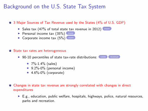
Background on the U.S. State Tax System
3 Major Sources of Tax Revenue used by the States (4% of U.S. GDP)
I Sales tax (47% of total state tax revenue in 2012) more
I Personal income tax (35%) more
I Corporate income tax (5%) more
State tax rates are heterogeneous
I 90-10 percentiles of state tax-rate distributions: rates revenue
F 7%-1.4% (sales)F 9.2%-0% (personal income)F 4.6%-0% (corporate)
Changes in state tax revenue are strongly correlated with changes in directexpenditures
I E.g., education, public welfare, hospitals, highways, police, natural resources,parks and recreation.
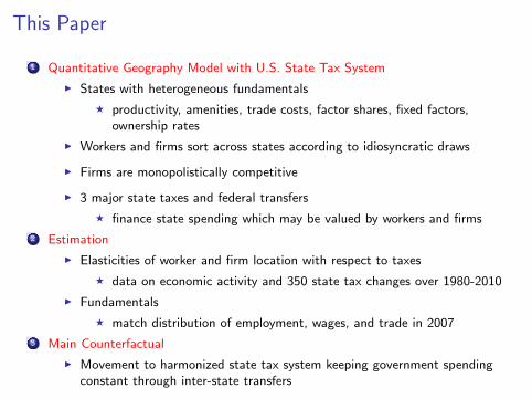
This Paper
1 Quantitative Geography Model with U.S. State Tax System
I States with heterogeneous fundamentals
F productivity, amenities, trade costs, factor shares, fixed factors,ownership rates
I Workers and firms sort across states according to idiosyncratic draws
I Firms are monopolistically competitive
I 3 major state taxes and federal transfers
F finance state spending which may be valued by workers and firms
2 Estimation
I Elasticities of worker and firm location with respect to taxes
F data on economic activity and 350 state tax changes over 1980-2010
I Fundamentals
F match distribution of employment, wages, and trade in 2007
3 Main Counterfactual
I Movement to harmonized state tax system keeping government spendingconstant through inter-state transfers

Literature
Misallocation
I Across firms: Restuccia and Rogerson (2008), Hsieh and Klenow (2009)I Across cities: Brandt et al. (2013), Desmet and Rossi-Hansberg (2013), Moretti
and Hsieh (2015)I Rural-Urban gaps: Gollin et al. (2013), Lagakos and Waugh (2013), Bryan and
Morten (2015)
Trade/Economic Geography
I Spatial equilibrium models: Roback (1982), Krugman (1991), Krugman andVenables (1995), Helpman (1998), Tabuchi and Thisse (2002)
I Quantitative geography model: Allen and Arkolakis (2014), Caliendo et al. (2014),Ramondo et al. (2015), Redding (2015), Gaubert (2015)
Public Finance/Urban
I Fiscal competition: Flatters et al. (1973), Gordon (1983), Oates (1999), Keen andKonrad (2013), Ossa (2015)
I Factor Mobility and Policy Changes: Bartik (1991), Holmes (1998), Moretti andWilson (2014), Suarez Serrato and Zidar (2015)
I General Equilibrium: Shoven et al. (1972), Ballard et al. (1985), Altig et al.(2001), Albouy (2009)

Model

Worker Utility and Location
Fraction of workers who choose region n :
Ln =⇣vnv
⌘"W
State-specific “appeal”:
vn = un
✓
Gn
L�Wn
◆↵W ,n✓
(1� Tn)wn
Pn
◆1�↵W ,n
where
1� Tn ⌘ (1� tyn ) (1� tyfed)� twfed1 + tcn
Representative worker’s utility:
v ⌘
X
n
v"Wn
!1/"W

Firms Profits and Location
Fraction of firms who choose region n:
Mn =
⇡n
�
z1n�
⇡
!
"F��1
where z1n = z1�↵F,nn
⇣
Gn
M�Fn
⌘↵F,n
Profits of firm with productivity z located in i :
⇡i (z) = max (1� t i )
NX
n=1
xni �NX
n=1
⌧niciz
qni
!
where t i = tcorpfed + t li +PN
n=1 txn sni
I Dispersion in sales apportionment leads to price distortion more
Immobile capital owners in state n own a fraction bn of a portfolio that includes allfirms and fixed factors
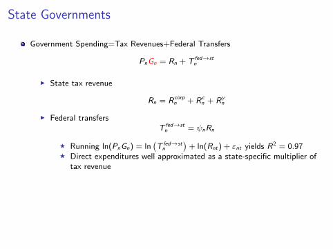
State Governments
Government Spending=Tax Revenues+Federal Transfers
PnGn = Rn + T fed!stn
I State tax revenue
Rn = Rcorpn + Rc
n + Ryn
I Federal transfersT fed!st
n = nRn
F Running ln(PnGn) = ln�
T fed!stn
�
+ ln(Rnt) + "nt yields R2 = 0.97F Direct expenditures well approximated as a state-specific multiplier of
tax revenue
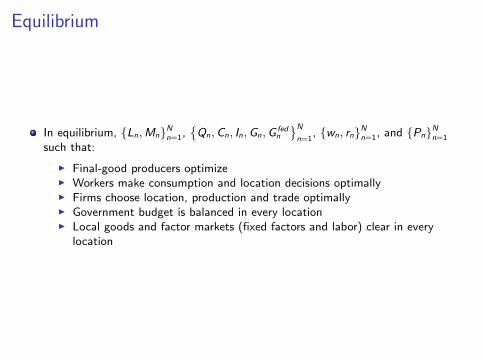
Equilibrium
In equilibrium, {Ln,Mn}Nn=1,�
Qn,Cn, In,Gn,G fedn
N
n=1, {wn, rn}Nn=1, and {Pn}Nn=1
such that:
I Final-good producers optimizeI Workers make consumption and location decisions optimallyI Firms choose location, production and trade optimallyI Government budget is balanced in every locationI Local goods and factor markets (fixed factors and labor) clear in every
location
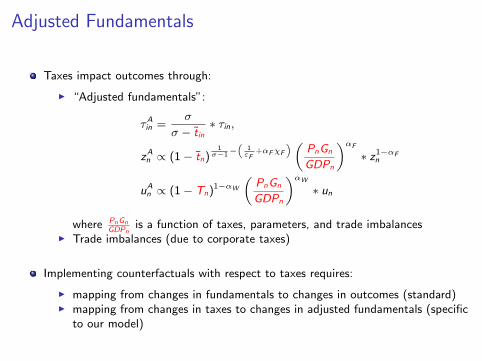
Adjusted Fundamentals
Taxes impact outcomes through:
I “Adjusted fundamentals”:
⌧Ain =�
� � tin⇤ ⌧in,
zAn / (1� tn)1
��1�⇣
1"F
+↵F�F
⌘ ✓PnGn
GDPn
◆↵F
⇤ z1�↵Fn
uAn / (1� Tn)
1�↵W
✓
PnGn
GDPn
◆↵W
⇤ un
where PnGnGDPn
is a function of taxes, parameters, and trade imbalancesI Trade imbalances (due to corporate taxes)
Implementing counterfactuals with respect to taxes requires:
I mapping from changes in fundamentals to changes in outcomes (standard)I mapping from changes in taxes to changes in adjusted fundamentals (specific
to our model)

Impact of Tax Dispersion on Worker Welfare
What is the e↵ect of eliminating dispersion in taxes {Tn} on worker welfare v keeping
{Gn} constant?
I Assume
F no trade frictions (⌧in = 1), perfect substitutes (� = 1), homogeneous firms("F= 1),
F no cross-state dispersion in income shares (�n = �) or in preferences forspending (↵W ,n = ↵W )
I Let Zn /�z0n/�n
�1/�n H�n�unG
↵Wn
�1/(1�↵W )and ⇣ ⌘ 1�↵W
1/"W+↵W�W+(1�↵W )�
Eliminating dispersion in{Tn} while keeping spending constant increases (decreases)
worker welfare if corr⇣Z⇣n , (1� Tn)
⇣⌘
is low (high) enough
Intuition
I Workers gain from dispersion in state-specific appeals, {vn}I State-specific appeal depends on both taxes and fundamentals (through prices)I High correlation between keep rates and fundamentals implies high dispersion
Consider corr⇣Z⇣n , (1� Tn)
⇣⌘= 0. Eliminating dispersion increases welfare if
(1� ↵W ) (1� �) > 1/"W + ↵W
I Holds for ↵W , �, �W large, "W small

Impact of Tax Dispersion on Real Income
Eliminating dispersion in {Tn} while keeping spending constant:
I may increase or decrease aggregate real income depending on the joint distributionof Tn, un, and Gn
I increases it under perfect mobility ("W ! 1), no public goods (↵W = 0), and nodispersion in amenities (un = 0)
F In this case, the model is the same as Hsieh and Klenow (2009)
Intuition
I Real income maximized under no dispersion of MPL.I But labor mobility is a↵ected by compensating di↵erentials,
v = unG↵Wn ((1� Tn)(MPLn))1�↵W

Key Forces
Agglomeration
I Home market e↵ects due to trade costs (final consumption andintermediates): {"W , "F ,�, {�n}}
I Returns to public spending: {↵F ,n,↵W ,n,�F ,�W }
Congestion
I Fixed factor used in production (land and structures): {�n}I Dispersed ownership of fixed factors: {bn}
Heterogeneity in productivity, endowments, amenities, trade costs: {zn,Hn, un, ⌧in}

Data and Estimation
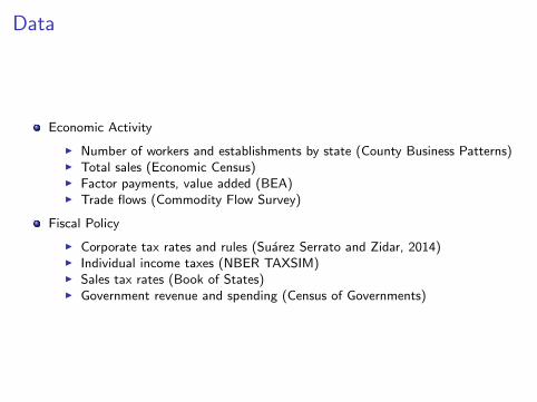
Data
Economic Activity
I Number of workers and establishments by state (County Business Patterns)I Total sales (Economic Census)I Factor payments, value added (BEA)I Trade flows (Commodity Flow Survey)
Fiscal Policy
I Corporate tax rates and rules (Suarez Serrato and Zidar, 2014)I Individual income taxes (NBER TAXSIM)I Sales tax rates (Book of States)I Government revenue and spending (Census of Governments)

Estimation Strategy
Elasticities of firm and worker location estimated from data on economic activityand taxes from 1980-2010
I {"W ,↵W ,n} estimated from labor-supply equationI {"F ,↵F} estimated using firm-mobility equation
Fundamentals, technologies, and ownership rates calibrated to (exactly) matchdata in 2007
I {zn,Hn, un, ⌧in} chosen to match spending shares, sales shares, employment,and wages details
I {�n,�n} match input and labor shares details
I {bn} match trade deficits details
Other parameters:
I Demand elasticity: � = 4 (Head et al., 2013)I {�W ,�F} 2 {{0, 0} , {1, 1}} (re-estimate in each case)

Estimation of {"W ,↵W}
Labor share in state n at time t:
ln (Lnt) ="W
�1� ↵W ,n
�
1 + �W "W↵W ,nln
✓(1� Tnt)
wnt
Pnt
◆+
"W↵W ,n
1 + �W "W↵W ,nln
✓Rnt
Pnt
◆+ L
t +⇠Ln+⌫
Lnt
I Identification assumption:
E[⌫Lnt | L, ⇠L,ZLnt ] = 0
I We use other-state taxes as instruments: ZLnt = (t⇤cnt , t
⇤xnt , t
⇤ynt )
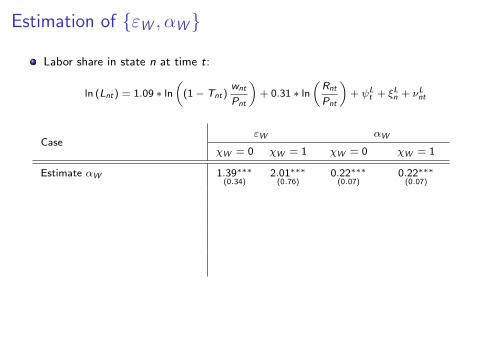
Estimation of {"W ,↵W}
Labor share in state n at time t:
ln (Lnt) = 1.09 ⇤ ln
✓(1� Tnt)
wnt
Pnt
◆+ 0.31 ⇤ ln
✓Rnt
Pnt
◆+ L
t + ⇠Ln + ⌫Lnt
Case"W ↵W
�W = 0 �W = 1 �W = 0 �W = 1
Estimate ↵W 1.39⇤⇤⇤(0.34)
2.01⇤⇤⇤(0.76)
0.22⇤⇤⇤(0.07)
0.22⇤⇤⇤(0.07)
Estimate ↵W ,n = ↵0 + ↵1POLn 1.24 3.08 [0.14, 0.18] [0.16, 0.17]
Assume ↵W = 0 1.04⇤⇤⇤(0.31)
1.04⇤⇤⇤(0.31)
Assume ↵F = 0.05 = 1N
Pn
RnGDPn
1.15⇤⇤⇤(0.32)
1.22⇤⇤⇤(0.36)
Assume ↵W ,n = RnGDPn
1.25⇤⇤⇤(0.36)
1.4⇤⇤⇤(0.49)

Estimation of {"W ,↵W}
Labor share in state n at time t:
ln (Lnt) = 1.09 ⇤ ln
✓(1� Tnt)
wnt
Pnt
◆+ 0.31 ⇤ ln
✓Rnt
Pnt
◆+ L
t + ⇠Ln + ⌫Lnt
Case"W ↵W
�W = 0 �W = 1 �W = 0 �W = 1
Estimate ↵W 1.39⇤⇤⇤(0.34)
2.01⇤⇤⇤(0.76)
0.22⇤⇤⇤(0.07)
0.22⇤⇤⇤(0.07)
Estimate ↵W ,n = ↵0 + ↵1POLn 1.24 1.57 [0.21, 0.22] [0.21, 0.23]
Assume ↵W = 0 0.93⇤⇤⇤(0.28)
0.93⇤⇤⇤(0.28)
Assume ↵F = 0.05 = 1N
Pn
RnGDPn
1.09⇤⇤⇤(0.31)
1.15⇤⇤⇤(0.35)
Assume ↵W ,n = RnGDPn
1.19⇤⇤⇤(0.35)
1.33⇤⇤⇤(0.45)

Estimation of {"F ,↵F}
Firm share in state n at time t:
lnMnt = 0.89 ⇤ ln ((1� tn)MPnt) + 0.14 ⇤ ln
✓Rnt
Pnt
◆� 2.69 ⇤ ln cnt + M
t + ⇠Mn + ⌫Mnt
Case"F ↵F
�F = 0 �F = 1 �F = 0 �F = 1
Estimate ↵F 2.70⇤⇤⇤(0.33)
3.15⇤⇤⇤(0.77)
0.05(0.06)
0.05(0.06)
Assume ↵F = 0 2.70⇤⇤⇤(0.61)
3.12⇤⇤⇤(0.45)
Assume ↵F = 0.05 2.67⇤⇤⇤(0.32)
2.67⇤⇤⇤(0.32)
details

Counterfactuals
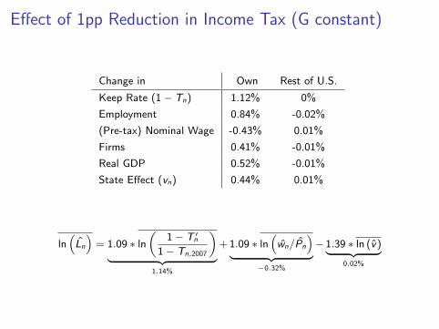
E↵ect of 1pp Reduction in Income Tax (G constant)
Change in Own Rest of U.S.
Keep Rate (1� Tn) 1.12% 0%
Employment 0.84% -0.02%
(Pre-tax) Nominal Wage -0.43% 0.01%
Firms 0.41% -0.01%
Real GDP 0.52% -0.01%
State E↵ect (vn) 0.44% 0.01%
ln⇣
Ln
⌘
= 1.09 ⇤ ln✓
1� T 0n
1� Tn,2007
◆
| {z }
1.14%
+1.09 ⇤ ln⇣
wn/Pn
⌘
| {z }
�0.32%
� 1.39 ⇤ ln (v)| {z }
0.02%

1pp Reduction in California’s Income Tax (G constant)
Figure : Employment Change (% points)
�������−��������������−��������������−��������������−��������������−��������������−�������&$� �����

Implementing Spending-Constant Counterfactuals
Goal: assess the impact of tax dispersion keeping government spending constant
I Replace�
tyn,2007, tcn,2007, t
ln,2007, t
xn,2007
withn
(ty )0 , (tc)0 ,�
t l�0, (0tx)
o
s.t.
⇣
t jn⌘0
= aj + b ⇤ t jn,2007
for n = 1, ..,N, j = y , c, l , x and aj , b � 0. fig.
I Keep government spending {Gn} constant through an inter-state transfersystem. I.e., for each b, find
�
aj
such that
NX
n=1
P 0nGn,2007 =
NX
n=1
R 0n +
⇣
T fed!stn
⌘0
Compute the change in aggregate real income and worker welfare,
bv =
X
n
Ln,2007bv"Wn0
!
1"W

Eliminating Tax Dispersion
Parametrization Constant Spending Variable Spending
↵W ,n ↵F Welfare GDP Welfare GDP
0.22 0.04 0.15% 0.12% 0.98% 0.92%
↵0 + ↵1POLn 0.04 0.15% 0.12% 0.96% 0.93%Rn
GDPn0.04 0.17% 0.12% 0.39% 0.94%
Rn0GDPn0
of random n0 6= n 0.04 0.17% 0.11% 0.38% 0.95%
0.00 0.00 0.20% 0.10% 0.16% 0.10%
0.22 0.00 0.16% 0.10% 0.48% -0.05%
0.00 0.04 0.19% 0.11% 0.44% 0.93%
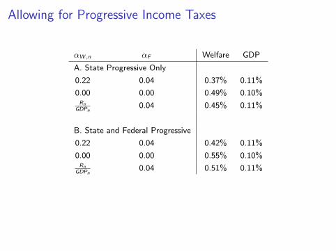
Allowing for Progressive Income Taxes
↵W ,n ↵F Welfare GDP
A. State Progressive Only
0.22 0.04 0.37% 0.11%
0.00 0.00 0.49% 0.10%Rn
GDPn0.04 0.45% 0.11%
B. State and Federal Progressive
0.22 0.04 0.42% 0.11%
0.00 0.00 0.55% 0.10%Rn
GDPn0.04 0.51% 0.11%
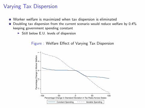
Varying Tax Dispersion
Worker welfare is maximized when tax dispersion is eliminated
Doubling tax dispersion from the current scenario would reduce welfare by 0.4%keeping government spending constant
I Still below E.U. levels of dispersion
Figure : Welfare E↵ect of Varying Tax Dispersion
-1-.5
0.5
1Pe
rcen
tage
Cha
nge
in W
orke
r Wel
fare
-100 -50 0 50 100Percentage Change in Standard Deviation in Tax Rates Across States
Constant Spending Variable Spending
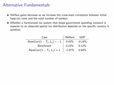
Alternative Fundamentals
Welfare gains decrease as we increase the cross-state correlation between initialkeep-tax rates and the total number of workers
Whether a harmonized tax system that keeps government spending constant issuperior to an observed spatial tax distribution depends on the specific country inquestion.
Case Welfare GDP
RankCorr(1� Tn, Ln) = �1 0.42% -0.14%
Benchmark 0.15% 0.12%
RankCorr(1� Tn, Ln) = 1 -1.07% 0.64%
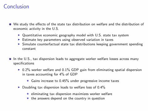
Conclusion
We study the e↵ects of the state tax distribution on welfare and the distribution ofeconomic activity in the U.S.
I Quantitative economic geography model with U.S. state tax systemI Estimate key parameters using observed variation in taxesI Simulate counterfactual state tax distributions keeping government spending
constant
In the U.S., tax dispersion leads to aggregate worker welfare losses across manyspecifications
I 0.2% worker welfare and 0.1% GDP gain from eliminating spatial dispersionin taxes accounting for 4% of GDP
F Gains increase to 0.45% under progressive income taxes
I Doubling tax dispersion leads to welfare loss of 0.4%
F eliminating tax dispersion maximizes worker welfareF the answers depend on the country in question

Distribution of Tax Rates Across States
0.1
.2.3
.4D
ensi
ty
0 5 10State Tax Rates in 2010
Sales Individual IncomeCorporate Sales Apportioned Corporate
back

Tax Revenue as Share of GDP Across States
90-10 percentiles of the distribution of sales, personal income, and corporate tax revenueshares: 76%-30%, 49%-0%, 8%-0%
0.0
2.0
4.0
6.0
8S
tate
Tax
Rev
enue
as
Sha
re o
f GD
P in
201
0
AK
DE
NH
WY TX SD
CO LA NV
OR
GA
TN VA
OK
MT IL
MO
WA
ND FL AZ
NE
UT
SC AL
OH IA NM
MD
NC PA
KS IN ID NJ
MA RI
CA
KY MI
CT
NY WI
VT
MN
AR
MS
ME
WV HI
Income Sales
Corporate
back

Dispersion in Sales Tax Rates Across States
Sales tax rates:
5 Highest Rates Rate 5 Lowest Rates Rate
California 8.25% Delaware 0%
New Jersey 7% Montana 0%
Mississippi 7% New Hampshire 0%
Tennessee 7% Alaska 0%
Indiana 7% Oregon 0%
Only final consumption is subject to sales taxes
I Firms do not pay sales taxes when buying intermediates
back
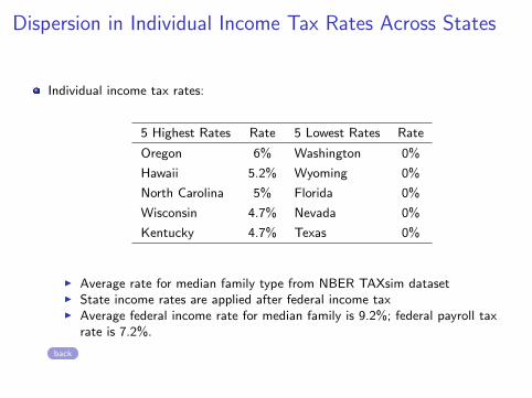
Dispersion in Individual Income Tax Rates Across States
Individual income tax rates:
5 Highest Rates Rate 5 Lowest Rates Rate
Oregon 6% Washington 0%
Hawaii 5.2% Wyoming 0%
North Carolina 5% Florida 0%
Wisconsin 4.7% Nevada 0%
Kentucky 4.7% Texas 0%
I Average rate for median family type from NBER TAXsim datasetI State income rates are applied after federal income taxI Average federal income rate for median family is 9.2%; federal payroll tax
rate is 7.2%.
back

Dispersion in Corporate Tax Rates Across States
Corporate tax rates:
5 Highest Rates Rate 5 Lowest Rates Rate
Iowa 12% Washington 0%
Pennsylvania 10% Wyoming 0%
Minnesota 10% Florida 0%
New Jersey 9% Nevada 0%
Rhode Island 9% Texas 0%
Applied on profits and apportioned through sales, payroll, and capital
I A single-plant firm j from i with export share s jni to state n pays:
F t li ⇡ji to state i , where t li = tcorpi ⇥ ✓li
F s jni txn⇡
ji to state n, where txn = tcorpn ⇥ ✓xn
F t j⇡ji in total, where t j = tcorpfed + t li +
P
n sjni t
xn
Internal trade matters for determining the corporate tax rate.
Federal corporate tax rate is 18%.
back
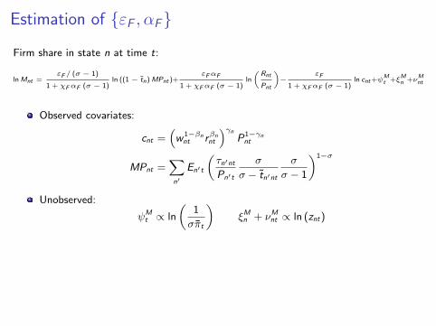
Estimation of {"F ,↵F}
Firm share in state n at time t:
lnMnt ="F / (� � 1)
1 + �F↵F (� � 1)ln ((1 � tn)MPnt )+
"F↵F
1 + �F↵F (� � 1)ln
✓Rnt
Pnt
◆�
"F
1 + �F↵F (� � 1)ln cnt+
Mt +⇠Mn +⌫Mnt
Observed covariates:
cnt =⇣
w 1��nnt r�nnt
⌘�nP1��nnt
MPnt =X
n0
En0t
✓
⌧n0ntPn0t
�
� � tn0nt
�� � 1
◆1��
Unobserved:
Mt / ln
✓
1�⇡t
◆
⇠Mn + ⌫Mnt / ln (znt)

Estimation of {"F ,↵F}
Firm share in state n at time t:
lnMnt ="F / (� � 1)
1 + �F↵F (� � 1)ln ((1 � tn)MPnt )+
"F↵F
1 + �F↵F (� � 1)ln
✓Rnt
Pnt
◆�
"F
1 + �F↵F (� � 1)ln cnt+
Mt +⇠Mn +⌫Mnt
Identification assumption:
E[⌫Mnt ⇤ (ZLnt ,MP⇤
nt , ⇠M , M)0] = 0
where
MP⇤nt =
X
n0 6=n
E⇤n0t
✓
⌧n0ntP⇤n0t
�
� � t⇤n0nt
�� � 1
◆1��
,
back
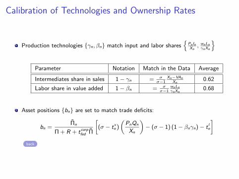
Calibration of Technologies and Ownership Rates
Production technologies {�n,�n} match input and labor sharesn
PnInXn
, wnLn�nXn
o
Parameter Notation Match in the Data Average
Intermediates share in sales 1� �n = ���1
Xn�VAnXn
0.62
Labor share in value added 1� �n = ���1
wnLn�nXn
0.68
Asset positions {bn} are set to match trade deficits:
bn =⇧n
⇧+ R + tcorpfed ⇧
(� � txn )
✓
PnQn
Xn
◆
� (� � 1) (1� �n�n)� t ln
�
back
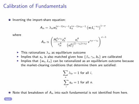
Calibration of Fundamentals
Inverting the import-share equation:
Ain = �inw(��1)1�1n L(��1)2n�1
n
�
wiL�3i
�1��
where
Ain /
H�n�nn zAn⌧Ain
uAi
�
uAn
�(1��n)+↵Fv↵F��n
!��1
I This rationalizes �in as equilibrium outcomeI Implies that sin is also matched given how {�n, �n, bn} are calibratedI Implies that {wn, Ln} can be rationalized as an equilibrium outcome because
the market-clearing conditions that determine them are satisfied:X
n
�in = 1 for all i ,
X
i
sin = 1 for all n.
Note that breakdown of Ain into each fundamental is not identified from here.
back
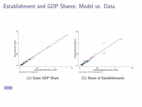
Establishment and GDP Shares: Model vs. Data
ALAZ
AR
CA
COCT
DE
FL
GA
HIID
IL
IN
IAKSKY LA
ME
MD
MAMI
MN
MS
MO
MTNE
NVNH
NJ
NM
NY
NC
ND
OH
OKOR
PA
RISC
SD
TN
TX
UTVT
VAWA
WV
WI
WY0.0
5.1
.15
Mod
el S
tate
GDP
Sha
re
0 .05 .1 .15Actual State GDP Share in 2007
Note: Slope is 1 (0). R-squared is 1.
(a) State GDP Share
AL AZAR
CA
COCT
DE
FL
GA
HIID
IL
IN
IAKS
KYLA
ME
MDMA
MI
MN
MS
MO
MTNENV
NH
NJ
NM
NY
NC
ND
OH
OKOR
PA
RI
SC
SD
TN
TX
UTVT
VAWA
WV
WI
WY0.0
5.1
.15
Mod
el E
stab
lishm
ent S
hare
0 .05 .1 .15Actual Establishment Share in 2007
Note: Slope is 1.01 (.04). R-squared is .92.
(b) Share of Establishments
back
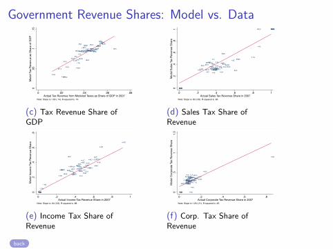
Government Revenue Shares: Model vs. Data
AL
AZ
ARCA
CO
CT
DEFL
GA
HI
ID
IL
IN
IA
KS
KY
LA
MEMD
MA
MI
MN
MS
MO
MT
NE
NV
NH
NJNMNYNCND OHOK
OR
PARI
SC
SD
TN
TX
UTVT
VA
WA
WV
WI
WY
0.0
5.1
.15
Mod
el T
ax R
even
ue a
s Sh
are
of G
DP
0 .02 .04 .06 .08Actual Tax Revenue from Modeled Taxes as Share of GDP in 2007
Note: Slope is 1.65 (.14). R-squared is .74.
(c) Tax Revenue Share ofGDP
AL
AZ
AR
CA
CO
CT
DE
FL
GA HI
ID
IL
IN
IA
KSKY
LAME
MD
MA
MI
MN
MS
MO
MT
NE
NV
NH
NJ NM
NYNC
ND
OHOK
OR
PA
RISC
SD
TN
TX
UT
VTVA
WA
WVWI
WY
0.2
.4.6
.81
Mod
el S
ales
Tax
Rev
enue
Sha
re
0 .2 .4 .6 .8 1Actual Sales Tax Revenue Share in 2007
Note: Slope is .83 (.05). R-squared is .85.
(d) Sales Tax Share ofRevenue
AL
AZ
AR
CA
CO
CT
DE
FL
GA
HI
ID
ILIN
IAKSKY
LA
ME
MDMA
MIMN
MS
MO
MT
NE
NV
NH
NJ
NM
NYNC
ND
OH
OK
OR
PA
RI
SC
SD
TN
TX
UT
VT
VA
WA
WV WI
WY0.2
.4.6
.8M
odel
Inco
me
Tax
Reve
nue
Shar
e
0 .2 .4 .6 .8 1Actual Income Tax Revenue Share in 2007
Note: Slope is .64 (.03). R-squared is .88.
(e) Income Tax Share ofRevenue
AL
AZAR CACOCT
DE
FLGA
HIID IL
INIA
KS KY
LA
MEMD
MA
MI
MN
MS
MO
MTNE
NV
NH
NJNM
NYNC
NDOH
OKORPA
RISC
SD
TN
TX
UT
VT
VA
WA
WVWI
WY0.5
11.
5M
odel
Cor
pora
te T
ax R
even
ue S
hare
0 .2 .4 .6 .8Actual Corporate Tax Revenue Share in 2007
Note: Slope is 1.29 (.21). R-squared is .45.
(f) Corp. Tax Share ofRevenue
back

Price Distortion
Sales apportionment leads to price distortion:
pni (z) = ⌧ni�
� � tni
�� � 1
ciz, where
where
tni =txn �
P
n0 txn0sn0 i
1� ti
I tni = 0 under no dispersion in sales apportionment across states (txn = tx forall n) back
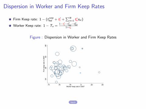
Dispersion in Worker and Firm Keep Rates
Firm Keep rate: 1� (tcorpfed + t li +PN
n=1 txn sni )
Worker Keep rate: 1� Tn =1�ttn�tyfed�twfed
1+tcn
Figure : Dispersion in Worker and Firm Keep Rates
.54
.58
.62
.66
Firm
kee
p ra
te in
200
7
.74 .76 .78 .8 .82 .84Worker keep rate in 2007
back