General rights Copyright and moral rights for the publications made accessible in the public portal are retained by the authors and/or other copyright owners and it is a condition of accessing publications that users recognise and abide by the legal requirements associated with these rights.

• Users may download and print one copy of any publication from the public portal for the purpose of private study or research. • You may not further distribute the material or use it for any profit-making activity or commercial gain • You may freely distribute the URL identifying the publication in the public portal

If you believe that this document breaches copyright please contact us providing details, and we will remove access to the work immediately and investigate your claim.

Downloaded from orbit.dtu.dk on: Jul 03, 2018

State-space solutions to the h_inf/ltr design problem

Niemann, Hans Henrik

Published in:International Journal of Robust and Nonlinear Control

Publication date:1993

Document VersionPublisher's PDF, also known as Version of record

Link back to DTU Orbit

Citation (APA):Niemann, H. H. (1993). State-space solutions to the h_inf/ltr design problem. International Journal of Robust andNonlinear Control, 3, 1-45.

INTERNATIONAL JOURNAL OF ROBUST AND NONLINEAR CONTROL, VOL. 3,1-45 (1993)

STATE-SPACE SOLUTIONS TO THE %/LTR DESIGN PROBLEM

JAKOB STOUSTRUP AND HANS HENRIK NIEMANN Mathematical Institute, Technical University of Denmark, Building 303, DK-2800 Lyngby, Denmark

SUMMARY The LTR design problem using an JC optimality criterion is presented for two types of recovery errors, the sensitivity recovery error and the input-output recovery error. For both errors two different approaches are presented. First, following the classical LTR design philosophy, a Luenberger observer based approach is proposed, where the Z part of the controller is appended to a standard full-order observer. Second, allowing for general controllers, an JC state-space problem is formulated directly from the recovery errors. Both approaches lead to controller orders of at most 2n. In the minimum phase case, though, the order of the controllers can be reduced to n in all cases. The control problems corresponding to the various controller types are given as four different singular state-space problems, and the solutions are given in terms of the relevant equations and inequalities.

KEY WORDS Loop transfer recovery Singular 25% theory Luenberger observer Youla parameterization

1. INTRODUCTION

In the last decade the concept of loop transfer recovery (LTR) has emerged as an important approach to the design of robust feedback controllers. The attractive theoretical properties of such controllers in combination with its conceptual and computational simplicity has motivated its popularity and spread in the control community for continuous time systems L45,8,11.18.19,?.4,25 and for discrete time system^.^"^.'^ The LTR philosophy establishes a systematic two-step method for the design of dynamical measurement feedback controllers. The first step is to design a static state feedback which performs according to the specifications. The second step is to design a dynamical measurement feedback controller, which ‘behaves almost’ like the static state feedback. In the two steps entirely different design methodologies can be applied, which make LTR an attractive alternative to ‘one-shot’ methods. The objective of this paper is to provide a complete % design method for the second step.

Design methods as LQGILTR, ES/LTR (i.e. eigenstructure assignment LTR) and singular perturbation LTR are all based on sufficient conditions for obtaining recovery. Further, practically only controllers based on full-order or minimal-order observers have been used for recovery design. As a result of these two drawbacks no guarantee can be given that the best controller type is selected for a given problem.

This work is supported in part by the Danish Technical Research Council, under grant no. 16-4885-1.

This paper was recommended for publication by editor M, J. Grimble

1O49-8923/93/01ooO1-45$27.50 0 1993 by John Wiley & Sons, Ltd.

Received 6 November 1990 Revised 20 February 1992

2 J. STOUSTRUP AND H. H. NIEMANN

A first step towards a more systematic description of conditions for obtaining recovery has been done by Goodman' by the introduction of the open loop recovery error for full order observer based controllers. In Reference 14 the recovery error concept has been extended to both open and closed loop recovery errors and more general controllers have been investigated: the Luenberger observed based controller and the output feedback controller (the unknown input observer based controller). In this work, it was shown that a certain matrix-valued function, the so-called recovery matrix, plays a crucial role in the LTR problem. In the asymptotic recovery case, it turns out that both recovery error types tend to zero if and only if the recovery matrix does. Accordingly, both necessary and sufficient conditions for achieving asymptotic recovery were obtained by the study of the recovery matrix.

Methods as LQG/LTR, ES/LTR and singular perturbation LTR are mainly ad hoc, in the sense that they try to reduce a more or less unspecified part of the system. In References 21 and 23 an Z / L T R problem is formulated in order to reduce the norm of the recovery matrix. We shall refer to this method as an indirect design method. One significant problem caused by using indirect design methods is that no guarantee exists that the norm of the recovery errors decreases when the norm of the recovery matrix decreases (except in the asymptotic recovery case-see above). In fact, in the course of this paper we shall study an example, where the recovery errors even increase when the norm of the recovery matrix decreases.

Moreover, for non-minimum phase systems, most contributions so far deal only with analysis. 17~1929 Hence, there is a need for systematic design procedures. A more advantageous approach to LTR controller design is therefore to use the recovery errors directly in the recovery design problem formulation, which we shall call the direct LTR design method. Till this point, only one such method has been investigated. l2 This recovery method imposes an Z constraint on the sensitivity recovery error. The method is based on coprime factorizations of the sensitivity recovery error for a system where the direct feedthrough term is assumed to have full rank. This method has two drawbacks: first, the order of the final observer based controllers is 2n for square system and 3n - 1 otherwise in the minimum phase case. However, it is always possible to reduce the Z norm of the recovery errors by nth order controllers in the minimum phase case. 21s23 Second, for non-minimum phase systems, only the minimum phase part is considered in Reference 12 and no norm bounds are guaranteed for the overall system. But, as a matter of fact, the main importance of direct design methods, are their application to non-minimum phase systems, as will appear in the course of this paper.

The key contribution of this paper is to formulate the recovery design problem as a direct Z optimization problem of the recovery errors and to derive the associated Z / L T R controller in state-space form. The basis of this contribution is the general recovery description given in Reference 14 which is summarized in Section 2. Concurrently, two different controller structures are considered for both the sensitivity recovery problem and the input-output recovery problem. First, the so-called Q-observer is considered which is a structure, where the Z part of the controller is appended (in a block-diagram sense) to a standard full order observer based controller. Second, a description is given, where the Z standard problem emerges directly from the recovery errors. 22 Effectively, five different 3% problem formulations are given at the end of Section 2.

The five Z problem formulated in Section 2, are all singular, i.e., they do not fulfil the usual assumptions about the rank of the direct feedthrough term. This problem is often overcome by approximation techniques, but a complete generalization of the Z problem to include singular D matrices have been given by Stoorvogel. 2o The results needed in this presentation are cited in Appendix A, along with some easy corollaries. In Appendix B the relevant algorithms for the singular Z approach are given.

.Xk./LTR DESIGN 3

In the following two sections (Sections 3 and 4) the solutions to the four direct ,% problems are given. State-space formulations of the 4% problems are given; the controllers are given in state-space form and are expressed in terms of certain quadratic matrix inequalities which are generalizations of the matrix Riccati equations known from Reference 3 (and solved by similar techniques).

The results from Sections 3 and 4 are briefly summarized in Section 5. In Section 6 an exhaustive discussion of a non-minimum phase example is given. Finally, some concluding remarks are given in Section 7.

2. THE LTR PROBLEM FORMULATION

In this section we shall shortly describe the significance of LTR and give a brief introduction of the Luenberger observer. Further, Q-parameterized controllers will be introduced, both as Luenberger observer based controllers and as general controllers.

2.1. The principle of recovery design

Loop transfer recovery (LTR) is a tool applied in robust multivariable control. LTR design is the last step in a two-step design procedure for constructing dynamic compensators. The first step in the procedure is a specification of the desired properties for the final feedback control system and the design of a target loop, using a state feedback for which the specifications are satisfied. Then the LTR step follows, where the target loop is ‘recovered’ by an admissible measurement based controller.

Suppose the design specifications are given as bounds on the sensitivity transfer function S( - ) and the complementary sensitivity transfer function T( - ).

where \I - 11- is the 4% norm. The performance specifications (e.g. asymptotic tracking, bandwidth) are expressed by the weight function W1( ) on the sensitivity function.’ The weight WZ( - ) on T( ) reflects system uncertainties such as disturbances, noise and modelling errors. In the sequel, the specifications will always be reflected to the input node. Independent of the selected dynamic controller type, see Sections 2.2-2.6, the systematic LTR design procedure can be applied to the design problem. First a state feedback design, the target design, which satisfies ( l ) , is designed, ‘.19 resulting in the target loop transfer function. Second, the LTR step is performed, where the target design is recovered systematically for each frequency by using a dynamic controller C(s). Often the system is assumed to be minimum phase, which has been shown to be a sufficient condition l4 for achieving asymptotic recovery, i.e. recovering each frequency arbitrarily well. The minimum phase condition is not necessary for asymptotic recovery. Necessary and sufficient conditions are known but rather complicated. The LTR design originated as an approach to design of full order observer based controller^,^'^ but it is possible to design other controller types by the LTR principle. l4 At this point we would like to stress, that the target design can be performed completely independent of the specific LTR procedure chosen. For non-minimum phase systems, though, it might in some cases be beneficial to design a state feedback which facilitates asymptotic recovery. l7

4 J . STOUSTRUP AND H. H. NIEMANN

2.2. Recovery errors

represented by a state-space realization (A, B, C, 0): Let us consider a finite-dimensional, linear, time-invariant (FDLTI) plant model,

=r=h+Bu z=cx with transfer function:

where xE IR", U E IRm,

G ( S ) = C(SI - A)-'B (3) z E R', with m > r and A, B and C are matrices of appropriate

dimensions. The system is assumed to be stabilizable, detectable and left invertible. Moreover, we shall make the technical assumption, that A(A) n 6 = 0. Note, however, that this can always be achieved by applying a preliminary static output feedback. Furthermore, this preliminary static output feedback can be chosen arbitrarily small.

The associated sensitivity and input-output transfer functions for the target design and the full loop design are given by:

(4)

( 5 )

&FL(S) = (I - F(s1- A)-'B)-'

SI(S) = (I - C(s)G(s))-'

where F is the target static state feedback, and C(s) is the controller to be designed. Using these transfer functions, two possible types of recovery errors can be defined.

Dejnition 2.1

The sensitivity recovery error ES and the input-output recovery error EIO are defined by

Es (s) = STFL(S) - SI (s)

EIO(S) = GFL(S) - GIO(S)

(8)

(9) The objective in the rest of this paper is to describe how the norm of these two recovery errors can be made small when applying different kinds of controllers, using methods. The various controller types will be introduced in the following.

2.3. The Luenberger observer based controller Suppose that we wish to control the plant by a control law of the form:

u = F%+ r = w + r (10)

where P is an estimate of the plant state. In the Luenberger observer w = F% is given by the following equations:

(1 1) = DZ + GU + Ey

w = Pz + v y

.%/LTR DESIGN 5

The Luenberger matrices T, D, E, G, P, V have to ~ a t i s f y : ~

(i) A(D)CC- (ii) TA - DT = EC

(iii) G = TB (iv) F =PT+VC

The controller obtained when applying this observer has the following transfer function:

(12)

C(s) = V + P(s1- D - GP)-'(E + GV), C ( s ) : p x m (13)

When the Luenberger observer based controller is applied, the two recovery errors of Definition 2.1 can be written in a more convenient form.

Lemma 2.2

Define

Then

Proof. The prool o

M ~ ( s ) = P(SI - D)-'G

Lemma 2.2 can be found in Reference 14.

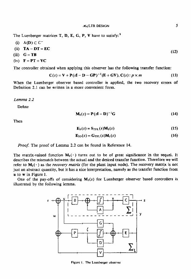
The matrix-valued function MI( * ) turns out to be of great significance in the sequel. It describes the mismatch between the actual and the desired transfer function. Therefore we will refer to MI( - ) as the recovery matrix (for the plant input node). The recovery matrix is not just an abstract quantity, but it has a nice interpretation, namely as the transfer function from u to w in Figure 1.

One of the pay-offs of considering MI (s) for Luenberger observer based controllers is illustrated by the following Iemma.

0 -

Figure 1. The Luenberger observer

6 J . STOUSTRUP AND H. H. NIEMANN

Lemma 2.3 With MI as above, then,

and

where ui( * ) is the ith singular value.

Proof. See Reference 26.

The two norm inequalities in Lemma 2.3 provide two measures of the relative mismatch between the full loop and the target loop, where 11 MI( ) 11.. is a common bound for these two measures (for all i). 11 MI( * ) 11- is therefore in a certain sense a measure for the quality of the recovery design. In 26 the strong dependency of the recovery design on )I MI(.) (1- has bLen used in analysing the trade-off between good recovery (i.e. small 11 MI( - ) and relatively low controller gains, which is inevitable for ‘generic’ systems. Moreover, the two inequalities also suggest that the task of reducing the norm of SI or Gro amounts just to the task of reducing 11 MI( - ) /I-, which is true in the minimum phase case (see 21 and 23). In Section 6, however, we shall give an example to illustrate, that EI or EIO is not always ‘minimized’ when MI is ‘minimized’.

In the following we shall use two special cases of the Luenberger observer, the full-order observer and the Q-observer.

2.4. The full-order observer

appears from the Luenberger expressions by the following selection of matrices: 9,15

The full-order observer is the most commonly used observer type. The full-order observer

D = A + K C G = B P = F E= -K v = o T = I

where K is the observer gain. The recovery matrix becomes:

MI(s) = F(sI - A - KC)-’B

for these Luenberger parameters.

2.5. The Q-observer

The second Luenberger observer based controller type to be considered in this section is the Q-parameterized controller implemented according to the construction in Reference 2. In the sequel we shall consider the reduction of the norm of the recovery errors in an A% framework.

.Y&/LTR DESIGN 7

To that end, we wish to compare the performance of controllers with a certain structure to that of general controllers, i.e., controllers that are only required to be FDLTI and internally stabilizing. One approach to characterize general controllers is the Youla parameterization of all stabilizing controllers. Briefly, the principle in the well-known Youla (or Q-) parameterization is to take any stabilizing controller which is thereafter fixed, and then make a certain interconnection structure. Now, the class of all stabilizing controllers is parameterized by applying the class of all &%, systems at the interconnection nodes. In Reference 2 it is shown that the simple construction shown in Figure 2 is an implementation of the Youla parameterization. In the sequel we shall us this implementation, which we shall denote the Q-observer.

In the following sections, we shall need the following result from Reference 14.

Lemma 2.4

Assume that Q E B%,, with a state-space representation, say,

XG = AQXQ + BQUQ ZQ = CQXQ + DQUQ EQ:

Here X Q E Rq, where q is the order of Q. Then the corresponding Q-observer is a Luenberger observer with the following parameters:

P = [F+ DQC CQ]

V = -DQ

The corresponding recovery matrix becomes:

MI(s) = F(sI - A - KC)-'B + Q(s)C(SI - A - KC)-'B (23)

2.6. The &%, standard setup

The traditional LTR design approach using observer based controllers, especially the Q-observer structure, has been treated in the above section. Alternatively, we can directly formulate the &%,/LTR design problem as an 31% standard problem. The Y& standard philosophy is to define a fictitious plant CT which is a realization of the compound transfer function on which the 3I% constraint is posed, rather than of the plant itself (see, for example, Reference 6).

Consider the closed loop system in Figure 3. Denote the transfer function of the controller C.s by Q(s) E 5W&. Then the closed loop transfer function from w to z becomes:

G d s ) = T d s ) + TZu(s)Q(s)(I - Tyu(~)Q(~))- lTyw(~) (24)

8 J . STOUSTRUP AND H. H. NIEMANN

I I ! w Z!TJ T

I c,! Figure 2. The Q-observer

z

Y U ?:g' Figure 3. The .% standard problem

where Tzw(s), TZU(s), Tyu(s) and Tyw(s) are the open loop transfer function from w - z, u - z, u - y and w - y respectively.

Now, with Gz,(s) being the sensitivity recovery error Es(s) introduced in Definition 2.1, we have:

Lemma 2.5

A linear fractional transformation of Es(s) in the form (24) is given by the following transfer functions:

T,,(s) = (I - F(SI - A ) - ~ B ) - ~ - I TzU(s) = - I Tyu(s) = C(SI - A)-'B T,(s) = C(SI - A)-'B

.%/LTR DESIGN 9

Proof. The proof is omitted. It follows directly from the definition of Es(s).

Similarly, for E~o(s) we have:

Lemma 2.6

A linear fractional transformation of EIO(S) in the form (24) is given by the following transfer functions:

T,,(s) = C(SI - A - BF)-*B - C(SI - A)-'B T,,(s) = -C(SI - A)-'B Tyll(s) = C(SI - A)-'B TYw(s) = C(SI - A)-'B

Proof. The proof is straightforward.

State-space representations for these two models of Es(s) and EIO(S) are given in Sections 3 and 4.

2.7. 3% formulation of the loop transfer recovery problem

turn out to have slightly different answers. The YG version of the LTR design problem can be stated in a number of ways which will

In References 21 and 23 the following problem was treated:

Problem 1

Let y > 0 be given. Find, if possible, a FDLTI system Q(s) such that:

I1 M I ( * llm < Y (27)

(28)

or, equivalently,

1 1 F(s1- A - KC)-'B + Q(s)C(sI - A - KC)-'B l l m < y

is achieved, and the closed loop system is internally stable. Here 11 * (IoD is the &?2, norm.

Thus, using the Q-observer structure in this formulation, the solution will immediately give us a Luenberger observer based controller, with the structure of Lemma 2.4.

For the asymptotic recovery case, any series of controllers which make the norm of MI(s) tend to zero, also make the norms of the two recovery errors in Definition 2.1 tend to zero. Consequently, we can just apply the simple procedure outlined in 21 and 23 for reducing MI( - ), even if the original goal was to reduce Es( * ) or EIO( * ). This will be called indirect design. The resulting controllers turn out to be of dynamic order not greater than n.

It might be, though that in the case where asymptotic recovery is not possible, we are in a situation where the norms of Es( * ) and EIO( - ) are not 'minimized' by the controller which 'minimize' the norm of MI ( * ). An example of this is given in Section 6. Hence, it is of interest to make a problem statement which directly involves the norms of Es( * ) and EIO( - ). This can be formulated either as a standard Z problem, or as a standard 3% problem where we furthermore require the solution to be in the Q-observer form.

10 J. STOUSTRUP AND H . H. NIEMANN

Problem 2

Q-observer the closed loop is internally stable, and: Let y > 0 be given. Find, if possible, a FDLTI system Q(s) such that when applied in a

II Es(- ) llm < Y or, equivalently,

1) (I + F(s1- A - BF)-'B)(F(sI - A - KC)-'B + Q(s)C(sI - A - KC)-'B) 11- < y (30)

The Q-observer expression for Es(s) and the following for Elo(S) has been derived in Reference 14. With no constraints on the controller type we get the following formulation.

Problem 3

a dynamic measurement feedback controller we achieve: Let y > 0 be given. Find, if possible, a FDLTI controller Q(s) such that when applied as

II Ed. ) llm < Y (31) or, equivalently,

( 1 F(sI - A - BF)-'B - Q(s)(I - C(s1- A)-'BQ(s))-'C(sI - A)-'B) < y (32)

is achieved, and the closed loop system is internally stable.

Problems 2 and 3 are treated in Section 3. Correspondingly, we consider the X, problem formulated for E I ~ , both with a Q-observer based controller, and directly as a standard problem.

Problem 4

Q-observer:

or, equivalently,

Let y > 0 be given. Find, if possible, a FDLTI system Q(s) such that when applied in a

(33)

(34)

I 1 EIO(.) l lm c Y

( 1 C(SI - A - BF)-'B(F(sI - A - KC)-'B + Q(s)C(sI - A - KC)-'B) ! I D o < y

is achieved, and the closed loop system is internally stable.

Problem 5

a dynamic measurement feedback controller we achieve:

or, equivalently,

11 C(s1- A - BF)-'B

Let y > 0 be given. Find, if possible, a FDLTI controller Q(s) such that when applied as

(34) II Era(-) llm < Y

- C(SI - A)-'B - C(SI - A)-'BQ(s)(I - C(SI - A)-'BQ(s))-'C(sI - A)-'B < y (36) is achieved, and the closed loop system is internally stable.

Problems 4 and 5 will be treated in Section 4.

.%/LTR DESIGN 11

Note that from the results of Reference 2, it follows that solvability of Problem 2 (resp. 4) is equivalent to solvability of Problem 3 (resp. 5) .

3. THE SENSITIVITY Z / L T R DESIGN PROBLEM

In the following we shall consider the sensitivity recovery problem formulated with an Z optimality criterion. Two different formulations will be considered, which both impose an S4%. norm constraint on the sensitivity recovery error. Following the approach of References 14, 21 and 23, observer based controllers will be studied, which possess the Q-observer structure introduced in Section 2 which is based on the Youla (Q-) parameterization (Problem 2). In Section 3.3, a more direct approach will be taken (Problem 3), where no preliminary compensator is introduced, and the optimization problem is formulated without restrictions on the controller structure. Hence, the latter follows strictly the 'standard problem' philosophy of Z theory, whereas the former is more conceptually clear from an LTR point of view, since the corresponding controllers simply are classical, full state, observer based controllers, augmented (in a block diagram sense) by the required S4%. dynamics. As a drawback this implies that the controller order is initially larger than the 'standard problem' controllers. Fortunately, though, the superfluous controller states can easily be dismissed, as will be shown in the sequel. For the Q-observer based .%, problem, the sensitivity error is affine in the controller, whereas the sensitivity error is a general linear fractional transformation for the Z standard problem formulation. In the course of this section it will turn out that the two controller types, solving the Z / L T R problem in the two formulations, will have significant similarities, and design methods will be given for each controller type.

3.1. Preliminaries and notation

In the following we shall subscribe extensively to the so-called singular 3% theory in the approach of Reference 20. An introduction to this approach as well as a summary of the most important results for our needs is given in Appendix A. The algorithms involved are described in Appendix B.

Briefly the principle in the approach of Reference 20 is the following. First, a certain quadratic matrix inequality is considered, which along with two algebraic constraints (rank conditions) guarantees uniqueness of a solution. Once this solution to the quadratic matrix inequality has been obtained, a new system is constructed through the full information transformation (see Appendix A). For this transformed system another inequality, the dual quadratic matrix inequality is considered, again with two associated rank conditions. Eventually, once the unique solution to the dual quadratic matrix inequality has been determined, the transformed system is itself transformed by a dual transformation, the full control transformation. It so happens that the doubly transformed system (1) has the same controllers as solution to the S4%. problem as the original system, and (2) is minimum phase. These two facts imply that after the two transformations the solution to the original problem is easily obtained - see Appendix A.

For further details of the applied singular X, approach please refer to Appendix A. Here we shall introduce some required concepts and notation. Consider the following dynamic system:

X = AX+ BU + EW X E R",u E IR'", w E IR9

Z E IR' D ~ w yEIRP (37)

z = C ~ X + D ~ u

12 J . STOUSTRUP AND H. H. NIEMANN

where A , B , E , C ~ , D I , C ~ and D2 are matrices of appropriate dimensions. Based on these matrices, we define the following two matrix valued functions:

1 A'P + PA + CTC2 + Y-~PEE'P PB + CFD2 [ B'P + DZC2 D ~ T D ~ AQ + QA' + EE' + -y-'QC;C2Q QC: + ED

C1Q + DIET D ~ D T

F,W =

WQ)= [ (39)

Then we shall say that P 2 0 is a solution to the quadratic matrix inequality if and only if the following three conditions are all satisfied:

F,(P) 2 0 (40)

(41)

["' - A - y-2EE'p - "1 = n + normrank C2(sI - A)-'B + D2, vs E C+ U Co (42) rank

where normrank M( ) is the maximal rank of M(s) over all s E C. An algorithm for finding P satisfying (40-42) is given in Appendix B. We also need to introduce the dual quadratic matrix inequality. We say that Q 2 0 is a solution to the dual quadratic matrix inequality if:

rank F,(P) = normrank C2(sI - A)-'B + D2

FAP)

Gy(Q) 2 0 (43)

rank G,(Q) = normrank Cl(sI - A)-'E + Dt (4)

G,(Q) = n + normrank Cl(s1- A)-'E + D1, Vs E C+ U C'

(45)

1 SI - A - Y - ~ Q C I C ~ - c1

rank [

3.2. Sensitivity recovery using the Q-observer

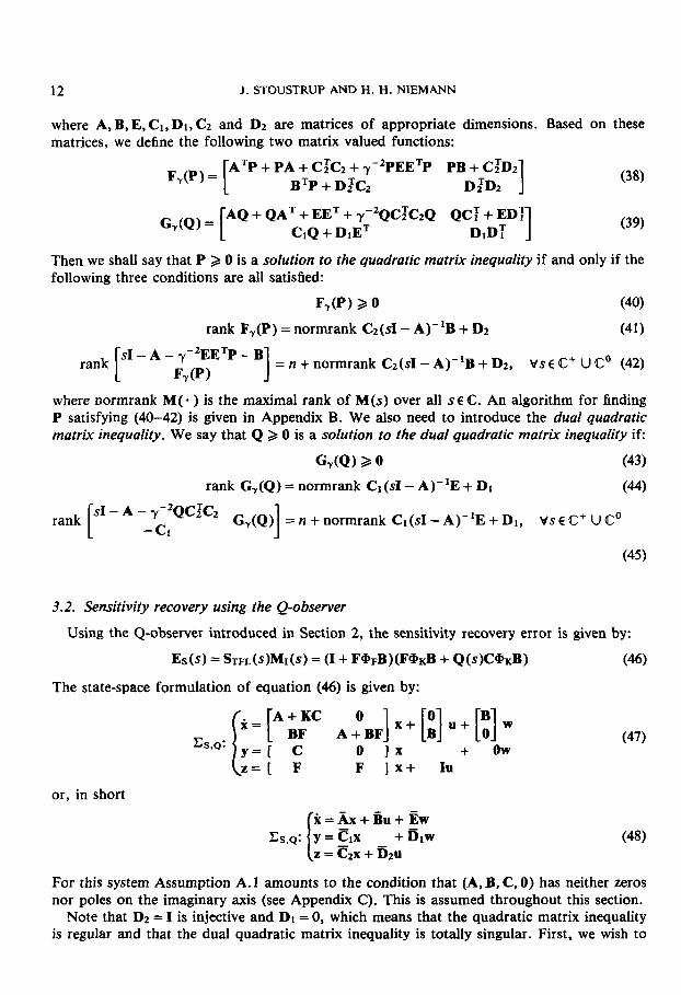
Using the Q-observer introduced in Section 2, the sensitivity recovery error is given by:

Es(s) = STFL(S)MI(S) = (1 + F@FB)(F@KB + Q(s)C@KB) (46)

The state-space formulation of equation (46) is given by:

( z = [ F F ] x + Iu

or, in short

x =Ax + Bu + Ew CS,Q: Y=elx + b l w (48) [ 2 = c2x + b2u

For this system Assumption A.1 amounts to the condition that (A, B, C, 0) has neither zeros nor poles on the imaginary axis (see Appendix C). This is assumed throughout this section.

Note that D2 = I is injective and DI = 0, which means that the quadratic matrix inequality is regular and that the dual quadratic matrix inequality is totally singular. First, we wish to

.%./LTR DESIGN 13

find a solution to the quadratic matrix inequality, so we can perform the full information transformation (see Appendix A). Using injectiveness of DZ to apply Corollary A.3 the solution to the quadratic matrix inequality is found:

Theorem 3.1

For the system CS,Q described by (47), the solution of the quadratic matrix inequality with the associated rank conditions, is:

F=[" O P o] (49)

where P is the unique solution to the algebraic Riccati equation:

A ~ P + PA - P B B ~ P = o (50)

P is given by: P = - llf(IIGJIT)-'ll

Here, G, is the controllability gramian, and ll is the orthogonal projection on to *A)* along Z(A), the space of generalized stable eigenvectors of A. - -

F,(P) factorizes as:

[F B T P + F I] = pp] [ ~ z , P bp] D;

Proof. See Appendix C .

Note that the solution of the quadratic matrix inequality does not depend on y. Further, in the special case when A is stable, F=O is the unique solution, and the resulting full information transformation (see Appendix A) in this case is the identity.

In general, performing the full information transformation (see Appendix A), we get the following matrices:

A p = A C1.P = el

bp = 0 2

(53) C2,p = [F BTP + F]

Now a solution P to the dual quadratic matrix inequality for the transformed system has to be found in order to determine the corresponding full control transformation. Using the dual of Corollary A.4 one can easily see that:

Lemma 3.2

solution of the associated dual quadratic matrix inequality, Let the matrices A P , B , E , E I , P , C ~ , P , ~ % and bp be as in (47), (48) and (53). Then the

14 J . STOUSTRUP AND H. H. NlEMANN

satisfies:

CY11=0 and CYl2=0 - - Gy(Y) factorizes as:

The conditions under which the dual quadratic matrix inequality has the solution P = 0 are different from the conditions under which the (primary) quadratic matrix inequality has the solution P = 0 as it is seen from the following corollary.

Corollary 3.3

Assume that the system (A,B,C,O) is invertible and minimum phase. Then P=O is a solution of the dual quadratic matrix inequality satisfying the involved rank conditions. Conversely, = 0 is a solution of the dual quadratic matrix inequality only if (A,B,C,O) is invertible and minimum phase. In this case no second (full control) transformation is needed.

Proof. See Appendix C.

For %? # 0 the full control transformation proceeds as follows:

with:

A ~ ! Q = AK + y-'YIIFTF + T-~Y]~(PBF + FTF) AsfQ = y-2Yll(FTBTP + F'F) + y-2Yi2(PBBTP + F'F) A$!Q = BF + y-2Yi2FTF + y-'Yi2(PBF + F'F) A~:Q = AF + T - ~ Y I ~ ( F ~ B ~ P + F'F) + ym2Y22(PBBTP + F'F)

and

After the full information and full control transformations (see Appendix A), the controller U = Q(s)y described in Theorem A.5 can now be designed in order to satisfy the two norm inequalities in (A.12) and (A.13). It is readily seen that (A.12) is trivially satisfied for:

L = -C2,p (58)

since this solves an (exact) disturbance decoupling problem.

Lemma 3.4

Let P be given by (51) and let M = [M: MT]' be any matrix satisfying

11 (SI - AP,Q - MCl,P)-'EP,Q 11- < y/ 11 C2.P 11 (59)

.Y&/LTR DESIGN 15

Then an admissible controller for the above a% problem is given by: - 1 SI - A - KC - MIC [ -M2C SI - A: BBTP] [::I Q(s) = [F BTP + F]

= F(s1- A - KC - MlC)-'Ml + (BTP + F)sI - A + BBTP)-'M2C(sI - A - KC - MiC)-'Ml + (BTP + F ) ( d - A + BBTP)-'M2 (60)

Proof. The lemma follows directly by substituting the above matrices in Theorem A.6.

The controller derived in Lemma 3.4 has dynamic order 2n. When inserted in the overall controller structure, as described in Section 2, we get a controller of order 3n, if no reduction is carried out. It turns out, though, that a structural reduction can be performed. The basic idea is to use the remaining freedom in the observer gain K designed in Section 2 to obtain some of the desired controller dynamics. This is done by means of a procedure as follows. First a full (nth-)order observer Cobs with any stabilizing gain K is designed. Using the Q-observer construction we append a dynamic compensator Ex, of order 2n such that the a% constraints are satisfied by the overall compensator. Now the original full order observer is returned, allowing for a dynamic compensator EL of order n to be substituted for CS-, maintaining the same transfer function for the cascade of the two compensators: the modified full order observer Ezbs and the modified a% controller EL, as we achieved for the original full order observer Cobs cascaded with the YG, controller CS&. - see Figure 4. The validity of the method described above, follows from Theorem 3.5.

(a) (b) Figure 4. (a) Original system with Jnth-order controller. (b) Transformed system with 2nth-order controller

Theorem 3.5

Let the transfer function Q * ( s ) for the output feedback compensator system C.>* be given by its transfer function Q*(s) = (B'P + F)(sI - A + BBTP)-'Mz. When applying Z,%- to a Q- observer configuration with observer gain K* = K + MI (see Figure 4(b)), the a% norm of the transfer function from w to z equals the YG, norm obtained when applying C . H ~ described by (47) to a similar system with observer gain K.

Proof. Please refer to Appendix C.

16 J. STOUSTRUP AND H. H. NIEMANN

In the minimum phase case it can be seen that an nth-order admissible controller is obtained by choosing M2 = 0. Mi must then satisfy:

11 (sI - A - KC - MIC)-'B 110. < y/ I( STFL(. IF IIm (61)

which follows directly from the statement of the sensitivity recovery design problem. Luenberger observer parameters in both the minimum phase and the non-minimum phase case is given in the following theorem.

Theorem 3.6

following matrices: The cascade of C:bs and C k (described above) is a

Non-minimum phase systems:

D = [A+KC+MIC M2C A - BBTP O I

P = F B'P+F]

E = [" &yl] v = o

.=[:I

Luenberger observer, described by the

Minimum phase systems:

D = A + KC + MiC

G = B

P = F

E = K + M i

v = o

T = I

Moreover, the closed loop transfer function obtained by applying this Luenberger observer has % norm smaller than y.

Proof. See Appendix C.

Note that the overall controller is of order n in the minimum phase case, and 2n in the non- minimum phase case. The reason, why the controller reduction from 3n to 2n is possible, is the remaining freedom in the preliminary observer design. The dynamics from this observer will be cancelled by the &%, controller and substituted by a more feasible one in the resulting Q-observer structure.

Note that only the output injection M in the %/LTR controller depends on y; L does not.

3.3. Sensitivity recovery in the % standard formulation

in Section 2.2 has the form in Section 2.6: When applying a general controller Q, Q c 5Z?.%, the sensitivity recovery error introduced

E ~ ( s ) = F(sI - A - BF)-'B - Q(s)(I - C(SI - A)-'BQ(s))-'C(sI - A)-'B (62)

which is a linear fractional transformation in Q(s) .

.%/LTR DESIGN 17

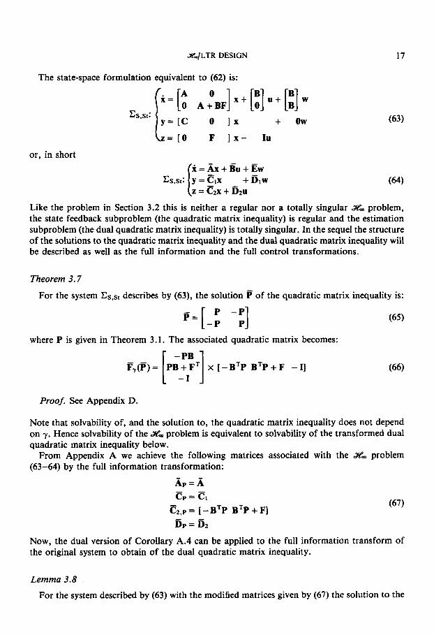
The state-space formulation equivalent to (62) is:

L = [ O F ] x - IU

or, in short x = Ax + Bu + Ew

Cs,st: y = ClX + b l W [ 2 = C2x + 62u

Like the problem in Section 3.2 this is neither a regular nor a totally singular A% problem, the state feedback subproblem (the quadratic matrix inequality) is regular and the estimation subproblem (the dual quadratic matrix inequality) is totally singular. In the sequel the structure of the solutions to the quadratic matrix inequality and the dual quadratic matrix inequality will be described as well as the full information and the full control transformations.

Theorem 3.7

For the system &.st describes by (63), the solution P of the quadratic matrix inequality is:

P - P p = [ - P PI 165)

where P is given in Theorem 3.1. The associated quadratic matrix becomes:

(66) - -

x [-BTP BTP+F -I]

Proof. See Appendix D.

Note that solvability of, and the solution to, the quadratic matrix inequality does not depend on y. Hence solvability of the 3% problem is equivalent to solvability of the transformed dual quadratic matrix inequality below,

From Appendix A we achieve the following matrices associated with the % problem (63-64) by the full information transformation:

& = A ep = e,

bp = 6 2

(67) Q p = [ - BTP BTP + F]

Now, the dual version of Corollary A.4 can be applied to the full information transform of the original system to obtain of the dual quadratic matrix inequality.

Lemma 3.8

For the system described by (63) with the modified matrices given by (67) the solution to the

18 J. STOUSTRUP AND H. H. NIEMANN

dual quadratic matrix inequality:

satisfies

in addition to the conditions (4) and (6) of Theorem A.2. c7(y ) factorizes as:

CYII=O and CY12=0

This time the special case = 0 appears in the following situation:

Corollary 3.9

solution to the dual quadratic matrix inequality, satisfying the involved rank conditions. Assume that the system (A,B,C,O) is invertible and minimum phase. Then i ! = O is a

Proof. Equivalent to the proof of Corollary 3.3.

For % # 0 the full control transformation proceeds as follows:

with:

A$!Q = A + y-2(Y11 - Y12)PBBTP - y-2Y12FTBTP A ~ ! Q = y-'(YT2 - Y22)PBBTP - Y - ~ Y ~ ~ F ~ B ~ P

A~:Q = AF + Y-~(Yzz - YT2)(PBBrP + PBF) + Y - ~ Y ~ ~ ( F ' B ~ P + FTF) A$:Q = ~ - ~ ( Y i z - Yii)(PBB'P + PBF) + y-2Yi2(FTBTP + FTF)

After these two transformations, the final controller Q ( s ) can be designed directly, by means of solutions to the two norm inequalities given by (A.12) and (A.13). It is readily seen that (A. 12) is trivially satisfied for:

L = [-BTP BTP+F] (72) since this choice solves an (exact) disturbance decoupling problem.

Lemma 3.10

Let P be as above and let M = [MT MI]' be an output injection satisfying:

I1 (sI - AP.Q - MG)-'EP,Q 11- < y/ II G,P I1 (73) Then an admissible controller for the above .%, problem is given by:

(74) SI - A + BB'P - MIC -BB'P - BF] -' E:] [ -M2C SI - A - BF

Q(s) = - [ - BTP B'P + F]

. Z / L T R DESIGN 19

Proof. Lemma 3.10 follows by substituting the above matrices in the expression of Theorem A S . The relaxed norm bound in (73) (compared to (A.12)) is achieved by exploiting that L solves an exact disturbance decoupling problem.

Note that the controller depends on Y only indirectly (through M).

is invertible and minimum phase. The following controller results from substituting Theorem A S .

As in Section 3.2 it is possible to obtain an nth-order controller if the system (A, B, C, 0) = 0 in

Lemma 3.11

admissible controller for the above A% problem is given by: Assume that v=O is the solution to the dual quadratic matrix inequality. Then an

(75) Q(s) = F(sI - A - BF - NC)-'N

Proof. See Appendix D.

4. THE INPUT-OUTPUT S&/LTR DESIGN PROBLEM

In this section we shall consider the input-output recovery problem with an ;>I&, optimality criterion. As in Section 3, two different approaches will be taken. In Section 4.1 the A% prob- lem is treated by the Q-observer formulation from Section 2, Problem 4. In Section 4.2 the problem is formulated with no constraints on the imposed controller type, the standard A% setup (Problem 5) .

4.1. Input-output recovery using the Q-observer

becomes: with the Q-observer structure introduced in Section 2, the input-output recovery error

EIO(S) = (;TFL(s)MI(s) = C(SI - A - BF)-'B(F(sI - A - KC)-'B + Q(s)C(sI - A - KC)-'B) (77)

The state-space model of the input-output

or, in short

L=[ 0

recovery error transfer function is:

A + B F O ] x + [ ; ] u + [ 9 w

0 I X + ow

c 3 x + ou

(78)

20 J. STOUSTRUP AND H. H. NIEMANN

The corresponding X2 problem is seen to be totally singular. Now, following the line of Section 3.1, the solutions to the quadratic matrix inequality and the dual quadratic matrix inequality are found, using Corollary A.4 and the associated transformations. For the quadratic matrix inequality we have the following.

Theorem 4.1

The quadratic matrix inequality associated with the system &O,Q has the solution

where P is the unique matrix satisfying:

(i) ATP + PA + CTC = CT,PC~,~ 2 0 (ii) PB = 0

(iii) rank (ATP + PA + CTC) = normrank G(s)

(iv) rank [” - A -”] = n + normrank G(s) , Vs E ct C2.P 0

with G ( s ) = C(s1- A - BF)-’B.

Proof. See Appendix E.

Note, that the quadratic matrix inequality in this case reduces to a dissipation inequality (known from classical LQG theory, see for example, Reference 7) of nth order. This equation can be solved by a much simplified version of the algorithm in Appendix B.

Also in the case the solution of the quadratic matrix inequality is independent of y. Solvability of the %/LTR problem will effectively depend only on solvability of the transformed dual quadratic matrix inequality.

As a consequence of Theorem 4.1 we have the following corollary.

Corollary 4.2

Assume that (A,B,C,O) is minimum phase. Then P=O is the unique solution to the quadratic matrix inequality. Conversely, if P = 0 solves the quadratic matrix inequality (and the associated rank conditions), (A, B, C, 0) is minimum phase.

Proof. Corollary 4.2 follows directly from Theorem 4.1.

In general, however, the full information transformation (see Appendix A) will be non-trivial, and amount to:

Ap= A C1.P = El (82) C2,P = [O C2,pl

On this system, obtained by the full information transformation, the dual version of Corollary A.4 can now be applied to derive the solution of the dual quadratic matrix inequality.

.%/LTR DESIGN 21

Lemma 4.3

modified as in (82), the solution: For the dual quadratic matrix inequality associated with the system CIO,Q with matrices

in addition to the conditions (4) and (6) of Theorem A.2. E,(v) factorizes as:

Er(P)= EQ] x [ETp,Q 01

Proof. The proof of Lemma 4.3 proceeds exactly as the proof of Lemma 3.2.

As in the sensitivity recovery error case, it will be possible to simplify the solution of the dual quadratic matrix inequality in special cases, as it appears from the following Corollary.

Corollary 4.4

to the transformed dual quadratic matrix inequality. If (and only if) the system (A, B, C, 0) is minimum phase and invertible, p = 0 is a solution

More generally, though, the full control transformation will result in the following matrices:

and B ~ , Q = B 1 y -2Y 12CT,PC2,P = [A+KC BF A + BF + y-2YzzCz,~C2,~

Performing both transformations, we eventually obtain the controller, solving the Z problem.

Lemma 4.5

Assume that y has been chosen sufficiently large. Let L = [L1 Lz] be a state feedback satisfying (A.12) and let M = [M: M i l T be an output injection satisfying (A.13). Then a controller, making the closed loop internally stable, and making the 2% norm of the transfer from w to z smaller than y is given by:

Q(s) = - [Li SI - A - KC - MiC - BF - BLI - M2C

- r-2Y '2CT.PC2,P SI - A - BF - y-'Y22CT,pC2,p - BL2 I-' x ["'I M2

(86)

Moreover, whenever a solution exists, it can be seen that L might always be chosen as L = [ - F Lz] . Hence, the problem can always be solved by applying a controller of the form:

[ Lzl X

SI - A - KC - MiC -M2C

- y-2Y12cz,Pc2,P Q W = [F -L21 X [ SI - A - BF - y-'Y22CT,pCz,p - BL2

Proof. (86) follows directly from Theorem A.5. L1 = - F is proven in Appendix E.

22 J . STOUSTRUP AND H. H. NIEMANN

The Q-term, given by (87), of the controller is of dynamic order 2n, which means that the complete controller will be of order 3n. In Section 3 it was possible by careful selection of the preliminary observer gain K to obtain a 2nth-order controller. AIso for the 10-recovery prob- lem, if the preliminary full order observer gain had been chosen as K* = K + MI rather than K, it can be shown that the resulting controller with 3n controller states would have had a transfer function of dynamic order 2n (when selecting M = [O M?] which is admissible in this case). In Section 3 this 2nth-order transfer function could itself be implemented as a Q- observer with an nth-order Q-term. This is not possible for the 10-recovery problem. However, the 2nth-order transfer function can still be implemented as a Luenberger observer based controller, whose parameters are given in Theorem 4.6. In the minimum phase case, Mz = 0 is an admissible choice which reduces the order of the controller to n. The minimum phase controller is now obtained by selecting MI such that:

1) (sI - A - KC - MiC)-'B !IoD < y<ll GTFL(' )F llOD)-' (88)

This is verified directly from the definition of the input-output recovery problem. The minimum phase controller can be implemented as a full order observer based controller with observer gain K*. In comparison we have:

Theorem 4.6

internally stabilizing and makes the S4% norm of EIO( 9 ) smaller than y: The Luenberger observer based controller with the following characteristic matrices is

Non-minimum phase systems: Minimum phase systems:

] D = A + K C + M , C D = [ A + KC + MIC y - 2Y12cT,Pc2,P MzC A + BF + BL2 + y-'Y22CESpC2,p

G = B

P = [F - L2] P = F

v = o v = o T = I

This Luenberger observer based controller, when applied to the system described by (78) makes the Z norm of the closed loop transfer function from w to z smaller than y.

Proof. The proof is given in Appendix E.

4.2. Input-output recovery in the S4% standard formulation

introduced in Section 2.2 has the form: When applying a general controller Q, Q E m,, the input-output recovery error

E , ~ = C(SI - A - BF)-'B - C(SI - A)-]B - C(s1- A)-'BQ(s)(I - C(s1- A)-'BQ(s))-'C(sI - A)-'B (89)

Yi%/LTR DESIGN 23

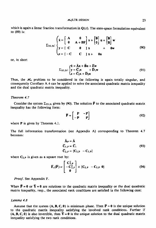
which is again a linear fraction transformation in Q ( s ) . The state-space formulation equivalent to (89) is:

\ Z = [ - C c ] x + ou or, in short

=Ax + Bu + Ew Cr0,st: y=C1x + b l W 1" z = c2x + bzu

Thus, the % problem to be considered in the following is again totally singular, and consequently Corollary A.4 can be applied to solve the associated quadratic matrix inequality and the dual quadratic matrix inequality.

Theorem 4.7

Consider the system 7210,s~ given by (90). The solution to the associated quadratic matrix inequality has the following form:

P -P p=[-P PI

where P is given by Theorem 4.1.

The full information transformation (see Appendix A) corresponding to Theorem 4.7 becomes:

& = A C1.p = c1

C2,P = iC2.P - C2,PI

where C2.p is given as a square root by:

F,(P) = -C;,P x iC2.p - C2.p 01 - - rpl

(93)

(94)

Proof. See Appendix F.

When P = 0 or v = 0 are solutions to the quadratic matrix inequality or the dual quadratic matrix inequality, resp., the associated rank conditions are satisfied in the following case:

Lemma 4.8

Assume that the system (A, B, C, 0) is minimum phase. Then P = 0 is the unique solution to the quadratic matrix inequality satisfying the involved rank conditions. Further if (A, B, C, 0) is also invertible, then = 0 is the unique solution to the dual quadratic matrix inequality satisfying the two rank conditions.

24 J. STOLJSTRUP AND H. H. NIEMANN

Proof. Follows from Theorem 4.7 and Theorem A.2.

These conditions are exactly the same as the conditions derived in Section 4.1. For non-trivial transformations we obtain the following matrices for the transformed system:

where:

Cl,P = El C2,P = K 2 , P -C2,p1

Eventually, an admissible controller, solving the 3iG problem is obtained in terms of these transformed matrices.

Lemma 4.9

Let L = [L1 Lz] be a state feedback satisfying (A.12) and let M = [MT MIIT be an output injection satisfying (A.13). Then, an internally stabilizing controller, making the 3iG norm of the closed loop transfer function from w to z smaller than y is given by:

Proof. Lemma 4.9 follows from (A.14).

In the case where the transfer function C(s1- A)-'B is minimum phase and square with full rank, then = = 0 and we have the following controller reduction.

Lemma 4.10

Assume that P = 0 and P = 0 are the solutions to the quadratic matrix inequality and the dual quadratic matrix inequality, respectively. Then an admissible controller for the above Z problem is given by:

(97) where N satisfies:

Q(s) = F ( d - A - BF - NC)-'N

1) ( ~ 1 - A - NC)-'B 11- < 7/11 Go(. )F 11- (98) with A + NC stable.

Proof. See Appendix F.

&/LTR DESIGN 2s

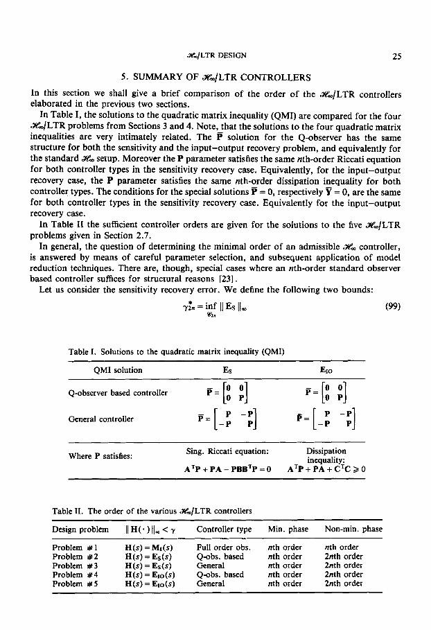
5 . SUMMARY OF Z./LTR CONTROLLERS

In this section we shall give a brief comparison of the order of the %/LTR controllers elaborated in the previous two sections.

In Table I, the solutions to the quadratic matrix inequality (QMI) are compared for the four Z / L T R problems from Sections 3 and 4. Note, that the solutions to the four quadratic matrix inequalities are very intimately related. The P solution for the Q-observer has the same structure for both the sensitivity and the input-output recovery problem, and equivalently for the standard Z. setup. Moreover the P parameter satisfies the same nth-order Riccati equation for both controller types in the sensitivity recovery case. Equivalently, for the input-output recovery case, the P parameter satisfies the same nth-order dissipation inequality for both controller types. The conditions for the special solutions = 0, are the same for both controller types in the sensitivity recovery case. Equivalently for the input-output recovery case.

In Table I1 the sufficient controller orders are given for the solutions to the five %/LTR problems given in Section 2.7.

In general, the question of determining the minimal order of an admissible 3% controller, is answered by means of careful parameter selection, and subsequent application of model reduction techniques. There are, though, special cases where an nth-order standard observer based controller suffices for structural reasons 1231.

= 0, respectively

Let us consider the sensitivity recovery error. We define the following two bounds:

= inf II ES [IDl (99) ra2.

Table I. Solutions to the quadratic matrix inequality (QMI)

QMI solution Es EIO

Q-observer based controller

General controller

P-=b ;] P -P

P-=[-P PI

Where P satisfies: Sing. Riccati equation: Dissipation inequality:

A ~ P + PA - P B B ~ P = o A ~ P + PA + C ~ C 2 o

Table 11. The order of the various &/LTR controllers

Design problem 11 H( * ) 11- < Controller type Min. phase Non-min. phase

Full order obs. nth order nth order Problem #1 Problem # 2 H 0) = Es 0) Q-obs . based nth order 2nth order Problem # 3 H(s) = Es(s) General nth order 2nth order Problem # 4 H(s) = E~o(s) Q-obs. based nth order 2nth order Problem # 5 H(s) = E~o(s) General nth order 2nth order

H (s) = MI (s)

26 J. STOUSTRUP AND H. H. NIEMANN

where the 'inf' is taken over all internally stabilizing FDLTI controllers of order no greater than 2n. Correspondingly, we define:

7; = inf 11 Es 11- (loo) W"

where the 'inf' is taken over all internally stabilizing FDLTI controllers of order no greater than n.

= $, we are guaranteed that an nth- order standard observer based controller will suffice. Otherwise controllers of order higher than n are required for near-optimal performance, in general.

In the special cases of a symptotic recovery, i.e. $n = 0, it can be shown that $= 7:n = 0. Necessary and sufficient conditions for obtaining asymptotic recovery are given in [14].

In Reference 12 the sensitivity recovery case has also been treated as an &2 problem. The approach in Reference 12 is based on frequency-domain methods, using coprime factorizations of the systems, and the solutions are found using the regular &2 theory. However, to make the A% problem regular, it has been necessary to consider plants including direct terms, i.e. plants given by:

Clearly 7:. < 7:. Only in the special case, where

G(s) = C(SI - A)-'B + D (101) where D has full column rank. When D does not have full column rank, only approximative solutions are given, whereas our results give exact answers. Further, the controller order in Reference 12 is 3n - 1 if no model reduction is carried out, whereas the order for the state- space approach based controllers introduced in this paper never exceed 2n. In the minimum phase case, our controllers are of order n, where the controllers in Reference 12 are of order 3n - 1 for non-square systems.

In the rest of this section, we will demonstrate how the presented &2/LTR design very easily can be extended to include non-strictly proper plants as given by (101), except that D is not required to have full column rank. In this case it is easily seen that the recovery matrix is:

M&) = F(SI - A - KC)-'(B + KD) + Q(S)C(SI - A - KC)-'(B + KD) (102) for non-strictly proper plants, when the Q-observer is used, Q E .%%%. The recovery error is then given by the following lemma.

Lemma 5.1

in (102). Then we get: Let the errors Es(s) and EIO(S) be as in Definition 2.1, and the recovery matrix MI(s) as

E ~ ( s ) = (I + F(sI - A - BF)-'B)(F(sI - A - KC)-'(B + KD) + Q(s)C(SI - A - KC)-'@ + KD)) (103)

(104) where Q E L%!%,,.

Solutions to the two more general problems associated with these expressions for Es(s) and EIO(S) can be obtained by straightforward extensions of the results in this paper. Note, that only the dual quadratic matrix inequality are modified. Instead of being totally singular they will be neither regular nor totally singular. For reasons of brevity, we shall not pursue this subject further here.

The standard &2 setup can equivalently be extended to handle non-strictly proper plants.

E ~ ~ ( s ) = (C + DF)(SI - A - BF)-'B(F(SI - A - KC)-'(B + KD) + Q(s)C(sI - A - KC)-'(B + KD))

%/LTR DESIGN 27

6. A NON-MINIMUM PHASE EXAMPLE

In this section we shall study an example of a non-minimum phase system to which the various controllers of this paper will be applied. We shall give comparisons of the recovery achieved by LQG/LTR controllers and %/LTR controllers designed by the four different techniques described in this paper. We shall consider design based on both types of recovery errors, which will also be compared to the %/LTR design which results from considering the recovery matrix, a design method which has been treated in References [21,23]. At this point, we would like to stress that the controller designs carried out in this section only aim to make the % norm for the specified problem 'very small'. Hence, we shall in all cases design controllers having closed loop performance very close to the infimally achievable % norm y*. This will in general have some drawbacks in terms of bandwidth etc., and in practice one wouldn't normally design controllers with y = y*. The example is, however, merely meant to illustrate the theoretical results and design methods outlined in this paper. y* is determined in the sequel by an iteration technique.

6.1. The recovery matrix

We shall consider the system given by the following state-space matrices:

1 , B = ["""I C = [l.ooOO -1.58111 -5 .5000 -0.6325 0.6325 O-oooO 0 . m ' A = [

This system has a right half plane zero, z = 1.0oO. As the target state feedback let us take:

F = [l.ooOO -8.95251

A standard LQG/LTR calculation gives the following observer gain:

- 22 453 .=[ 5797 ] Applying the LQG/LTR controller the maximal singular value of MI (s) becomes 1 - 3 5 - 2.62 dB. For the 3% problem described in References [21, 231, the infimally achievable y&, norm is y* = 0.67 - - 3.36 dB, and we can hence improve the LQG/LTR design by 6 dB by the technique described in References [21, 231. As a bound for the % problem we have to select y > y* so we choose, for example, y = 0-68 - - 3.35 dB.

By the technique outlined in References [21, 231, we find:

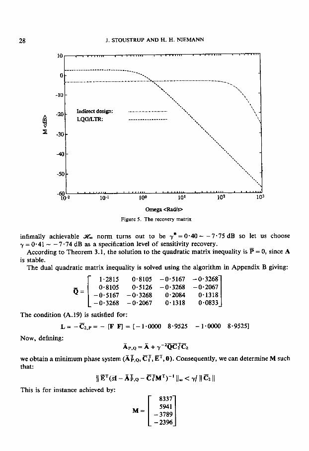
to satisfy the % bound. The recovery matrices achieved by applying these two second-order controllers are shown

in Figure 5 . The % plot has a maximum peak which is 6 dB lower than the maximum peak of the LQG plot. However, because of the restricted freedom of a second-order controller this gain in recovery level is paid for by a higher roll-off frequency.

6.2. The sensitivity recovery error

With the above system, we consider the problem of minimizing the sensitivity recovery error by means of a Q-observer based controller as described in Section 3. For this problem, the

28 J. STOUSTRUP AND H. H. NIEMANN

E

10-2 lo-' 100 10' 102 103 -601 ' ' """' ' ' """' ' ' """' ' ' """' ' '

Omega <Rad/s> Figure 5 . The recovery matrix

infimally achievable Z, norm turns out to be y* = 0.40 - - 7.75 dB so let us choose y = 0.41 - - 7.74 dB as a specification level of sensitivity recovery.

According to Theorem 3.1, the solution to the quadratic matrix inequality is F = 0, since A is stable.

The dual quadratic matrix inequality is solved using the algorithm in Appendix B giving:

I 1.2815 0.8105 -0.5167 -0.3268 0.8105 0.5126 -0.3268 -0.2067

Q = [ -0.5167 -0.3268 0.2084 0.1318 -0.3268 -0.2067 0.1318 0.0833

The condition (A.19) is satisfied for: -

L = -C2,p= - [F F] = [-l.ooOO 8.9525 -1.ooOO 8.95251

Now, defining:

we obtain a minimum phase system (A$,Q, CT, Ef, 0). Consequently, we can determine M such that:

AP*Q = A + y-YjCZC2

I ) ET(d - A$,Q - E:MT)-' 11- < y/ 11 C2 11 This is for instance achieved by:

&/LTR DESIGN 29

and the controller becomes:

Q(s) = C~(SI - A + BC2 - MCi)-'M

Now, let us consider the solution to the same problem in the standard formulation in Section 3.3. Of course the infimally achievable Sf& norm is the same in either formulation so we choose the same y as above as our specification.

Since A is stable, according to Theorem 3.7, P = 0 is the unique solution to the quadratic matrix inequality. For the dual quadratic matrix inequality we apply Algorithm B. 1 to obtain:

1 1.2815 0.8105 0.7648 0.4837 0-8105 0.5126 0.4837 0.3059

Q = [ 0-7648 0.4837 0.4564 0.2887 0.4837 0.3059 0.2887 0.1826

From (72) we obtain:

L = [0 F] = [O*oooO O.oo00 1 .oooO -8.95251

Calculating:

Ap,Q = A + we are able to determine M such that:

Since an almost disturbance decoupling problem is solvable for the transformed system. One possible choice is:

- 1464 M=[-;:3E] The resulting controller is:

Q ( S ) = -C*(SI -A - BE2 - M E ~ M

Figure 6 shows the sensitivity recovery errors achieved by applying these two fourth-order controllers compared to the two second-order controllers given above.

The two fourth-order controllers both have max peaks close to y which is an improvement of 6 dB and 7 dB compared to the LQG controller and the 'MI minimizing' controller, respectively. Note that the discrepancies in achieved Z, norm is not due to the different controller orders, but simply illustrates the fact that, when design is based on an Sf& bound for MI, we are not guaranteed anything about the Z, norm of Es.

6.3. The input-output recovery error For the A% problem described by (78) the corresponding fourth-order quadratic matrix

inequality can by Theorem 4.1 be reduced to a second-order dissipation inequality, which in Algorithm B.l reduces to a scalar quadratic equation. y* equals 0.11 - - 18.6 dB. Let US

30

-50

3. STOUSTRUP AND H. H. NIEMANN

- '. '. \

Q-observec Standard H-inf.: Indinct design: LQG/LTR: __-_-_____-__-___

.._ . . ... . _._........._... , .... . ...

choose y = 0.12 - - 18.4 dB. We get:

0 0 0 .=[o 0 0 0 0 0 i ]

0 0 0 4.9995

The dual quadratic matrix inequality is solved by Algorithm B.l and yields:

0.8172 0.5169 -0.3295 -0.2084 0.5169 0.3269 -0.2084 -0.1318

Q = [ -0.3295 -0.2084 0.1329 0.0840 -0.2084 -0.1318 0.0840 0.0532 1

We perform the transformations and obtain the following solutions to the almost disturbance decoupling problem and the almost disturbance decoupled estimation problem,

L = [-l.ooOO 8.9525 -383.4 -602.21 resp.M=

Note that I, = [ -F I,?] as stated in Lemma 4.5. For the general controller structure of Section 4.2, the 4% problem associated with Ero, the

%/LTR DESIGN

-100

31

-

,

Or 1 1 , 1 ,,,,, , , , , , , . , , , , . . . . . . . , . . . . . . . . . . . _ _ _ _ -

Standard H-inf.: Indirect design:

-80 t

..__ I

\ I

quadratic matrix inequality has the following solution:

0

0 0 0 P -P 0 4.9995 0 -4.9995

0 -4.9995 0 4.9995 P"-P 0 0

which is effectively obtained by solving a scalar quadratic equation, when Theorem 4.7 is applied. The dual quadratic matrix inequality has the following solution:

0-0266 0.0168 0.0159 0.0100 0-0420 0.0266 0.0251 0.0159

Q = [ 0.0251 0.0159 0.0150 0.0095 0.0159 0*0100 0.0095 0.0060 1

We perform the transformation, and achieve the following two gain matrices associated with the controller given by Lemma 4.9:

39 142

L = [ - 1276 - 2024 1277 20151 and M = [ z:] The input-output recovery achieved by these two fourth-order controllers is displayed in

Figure 7. Also the recovery of the two second-order controllers of Section 6.1 is shown. This time the fourth-order controllers have an % norm which is 2.7 dB better than the second- order controller and 5.4 dB better than the LQG controller. Again, the improvement is not

32 J. STOUSTRUP AND H. H. NIEMANN

due to the extra dynamics but is explained by the fact, that the fourth-order controllers aimed directly at a good input-output recovery.

6.4. Conclusions concerning the example

As our main conclusion, let us emphasize that a compensator solving a control problem, performs in accordance with the specifications for which the problem was posed, and the behaviour concerning different specifications might be arbitrarily bad in general. Hence, if we wish a closed loop system to have good sensitivity recovery, for example, the control problem should be stated as a sensitivity recovery problem, since a recovery matrix reduction does not yield any specific guarantees for the sensitivity recovery in the non-minimum phase case.

In the example, a controller which ‘minimizes’ the Z, norm of M,(s) gives a better input-output recovery than the LQG controller, but a (slightly) worse sensitivity recovery. Both controllers, though, behave considerably worse than the dedicated Z, controllers in both cases.

Another matter is the question of controller order. In the authors’ opinion the best way to achieve an nth-order controller, in the case where no specific simplifying conditions such as described in Sections 3 and 4 exist, is to design a 2nth-order dedicated controller and then perform frequency-weighted model reduction. It should be noted, however, that the best approach to this, is to start with a y which is not to close to y*. Otherwise, the states of the 2nth-order controller all tend to get ‘important’, as computing experience with the above example has shown.

7. CONCLUSIONS

In this paper we have given a precise formulation of the Z,/LTR problem based on the sensitivity recovery error and the input-output recovery error, where the & constraint has been imposed directly on these recovery errors.

The &/LTR problem has been treated in two ways: (1) in a straightforward fashion allowing for a general controller structure, and (2) with the constraint that the controller should be a Q-observer based controller as described in Reference 2. The Q-observer structure allows the Z, contribution to the controller to be appended (in a block-diagram sense) to a standard full-order observer based controller, which is appealing from a practical point of view.

The four resulting controllers are given in terms of the unique solution to the dual quadratic matrix inequality of order 2n, and additionally by the solution to an nth-order (singular) matrix Riccati equation (the two sensitivity cases) or, respectively, a nth-order dissipation inequality (the input-output cases). By the algorithms in Appendix B, the quadratic matrix inequality is in turn reduced to a reduced order matrix Riccati equation. Let us emphasize that all resuIts in this paper are completely constructive, and controllers can be found using well- known computational techniques.

Comparing the &%/LTR design methods proposed above to traditional LTR methods, a major advantage is that non-minimum phase systems can be treated by exactly the same techniques as minimum phase systems after a preliminary transformation has been performed. This preliminary transformation involves a state-space transformation and the solution to a reduced order Riccati equation. The preliminary transformation is a one-shot process requiring no iterations.

The four controllers considered in this paper are all of dynamic order at most 2n in the non- minimum phase case. For the controllers, though, a reduction can be carried out if the system

%/LTR DESIGN 33

considered fulfils a minimum phase condition (although the reduction is possible also for certain non-minimum phase systems) yielding an nth-order standard full-order observer based controller structure.

As it has been mentioned in Section 6, nth-order controllers can also be achieved by doing frequency-weighted model order reduction (which should probably emphasize cross-over frequencies). But, if model order reduction is intended from the start, the recovery specification level y should not be chosen too close to the infimally achievable value y*, since this tends to make the condition numbers of the gramians small, i.e. the smallest singular values become important to the design as well as the larger ones.

Not surprisingly the LQG controller does not compete with the a& controllers in the example of Section 6, when the maximal singular values are considered. This is rather obvious, owing to the fact that when a controller is designed with a certain optimality criterion it will behave optimal with respect to that criterion, and arbitrarily bad for other criteria. There are, though, some good reasons for applying the YC, norm as opposed to other norms to LTR prob- lems, since LTR typically is the last step in an overall design procedure, where the first step is robustness loop shaping. But to design for robustness the design objective must be posed in the YC, norm.

On closing, it is important to note some of the limitations of an automatic design procedure such as the one described in this paper. First of all, we have not been dealing with the first part of the design procedure, the state feedback design. For uncertain systems one should pay attention to the fact that not all robustness properties are guaranteed simply by the use of state feedbacks. State feedbacks themselves have to be designed such that the knowledge of the uncertainty structure is exploited. Then in our approach robust stability with respect to unmodelled dynamics is preserved in the dynamic output feedback controller implementation. Other kinds of uncertainties have to be taken care of separately. Finally, in this paper we have studied the a& norm of two recovery errors. In some practical applications, the given control objective is instead to reduce the norm of the recovery errors in certain frequency windows only. Hence, it would be relevant to incorporate weighting functions for the recovery errors in the theory. This can be done of course. However, the price is twofold. First, the order of the controllers will be even higher than 2n. Second, part of the structure of the solutions will vanish, implying that the algorithms will be slightly further complicated. Thus, a subject for further research is to consider weighed recovery errors by lower-order controllers.

APPENDIX A The required preliminaries for the method used in this paper will be introduced in this appendix. The approach taken is based on the results in Reference 20, the so-called singular X2 approach. This is a very general approach which includes the well-known approach by Doyle et

In the state-space approach to SL the standard problem is as follows. Consider a finite-dimensional, linear, time-invariant system:

as a special case.

X = A x + B u + E w xER", u E R m , w € R q y = C l x + Dlw y € R p z = C ~ X + D ~ u X € lRr

We assume that y > 0 has been given. We wish to design, if possible, an internally stabilizing FDLTI compensator u = Q(s)y such that the 3% norm of the resulting closed loop transfer function from w to z is smaller than y.

Assumption A. I

It is assumed that the systems (A, B, Cz, D2) and (A, E, CI, DI ) have no invariant zeros in Co.

34 J . STOUSTRUP AND H. H. NIEMANN

The main result is:

Theorem A.2

Consider the system C above satisfying Assumption A.l. Let y > 0 be given. Then, there exists a FDLTI compensator u = Q(s)y for which the SfL norm of the resulting closed-loop transfer function from w to z is smaller than y, if and only if there exist P a 0 and Q 2 0 for which:

(1) F,(P) 2 0 (2) G,(Q) 2 0 (3) rank F,(P) = normrank G (4) rank G,(Q) = normrank H

(5 ) rank [".". ''1 = n + normrank G , V S € C+ U Co F,(P)

(6) rank [M,(Q, s) G,(Q)] = n + normrank H, VSE C+ U Co (7) p(PQ) < y2

where the notation used is as follows:

1 I

A ~ P + PA + cIc2 + y - 2 ~ ~ ~ T ~ PB + CTDZ F,@) = [ BTP + D;cz D:D~

AQ + Q A ~ + E E ~ + y - Z ~ ~ ; ~ z ~ QCT + ED: G ~ ( Q ) = [ c l Q + DIET D ~ D T

1 SI - A - y-'QCZC2 L,(P, S) = [sI - A - y-'EETP - B] , M,(Q, s) =

(A.3)

('4.4)

G ( s ) = C~(SI - A)-'B + Dz, H(s) = CI(SI - A)-'E + DI (A.5) The proof of Theorem A.2 can be found in Reference 20. We shall refer to condition (1) as the quadratic matrix inequality, and any P a 0 satisfying (1) will be called a solution to the quadratic matrix inequality. Analogously we shall call (2) the dual quadratic matrix inequality, and refer to as solutions to the dual quadratic matrix inequality any Q 3 0 satisfying (2). Conditions (3) and ( 5 ) guarantees that a solution to the quadratic matrix inequality is unique and of minimal rank (and dually for the dual quadratic matrix inequality with (4) and (6)). (7) is a typical % coupling condition, which also appears in Reference 3.

Further, we shall need a couple of corollaries.

Corollary A.3. The regular case Assume that DZ in injective. Then (l), (3) and ( 5 ) are satisfied if and only if

A ~ P +PA + cIcz + y - 2 ~ ~ ~ T ~ - (PB + cTD~) (DTD~) -~ (B~P + DZC~) = o and

A(A + - B(D:D~) -~ (B~P + D%)) c c-

Corollary A.4. The totally singular case Assume DZ = 0. Then (1) is equivalent to:

A ~ P + PA + cTcz + y - z ~ ~ ~ T ~ 2 o where P satisfies PB = 0.

The two corollaries have straightforward duals, which are also used in this paper.

transformations of C. First we defined C2.p and Dp by the following factorization: Expressions for admissible controllers will be given in the following in terms of the matrices for certain

F,(P) = [G.P DplT x [CZ.P DPI (A. 6)

%/LTR DESIGN 35

Moreover, we will need the following matrices:

Ap = A + y-’EETP, CI,P = CI + y-’DIETP (A.7) Y = (1 - r - z ~ ~ ) - l ~ (A.8)

(A. 9) We shall refer to the system where AP, CI.P, CZ,P and DP substitute A, CI, CZ and DZ as the full

information transformation of the system C. The dual quadratic matrix inequality for the system obtained by the full information transformation becomes:

AP,Q = AP + y-zYC:,~Cz,~, BP,Q = B + y-’YC:,pDp

A ~ Y + YA$ + EE’ + y-z~c~ ,pcz ,p~ YC:,~ + C ] , ~ Y + D , E ~ = [ E ~ . Q D$.Q]’ X [E$,Q D$.Q] 2 0

(A.lO)

d,(Y) =

Substituting A ~ , Q , B ~ , Q , EP,Q and DP,Q for the corresponding variables in the previous system will be referred to as the full control transformation. The system obtained by the full control transformation becomes:

X = AP~QX + BP,QU + EP,QW CP,Q: y = c1 ,Px + DP.QW [ z = C2,px + D ~ u

In terms of these transformed system matrices we can compute the desired % controller:

(A. 11)

Theorem A.5

such that: Let AP,Q, Bp,q and C1.p be as above. Let L be a state feedback, such that AP,Q + BP~QL is stable, and

(A.12) I( WZ.P + DpL)(sI - AP,Q - BP,QL)-’ 11- < 7/(3 * 11 EP,Q 11 1 Let M be an output injection, such that AP,Q + MC1.p is stable and further:

I( (sI - AP,Q - M C 1 , ~ ) - ’ ( E p . ~ + MDP,Q) 11- < f (A.13) where

5 = min [y/(3 (I DPL I1 1, 11 EP,Q 11/11 BP.QL 11 I

u = - L(s1- AP,Q - BP,QL - MCI,P)-’MY (A. 14)

makes the .%% norm of the resulting closed loop transform function from w to z in C smaller than y.

The significance of Theorem A S is to transform the original &%. problem to two disturbance attenuation problems, which can be solved by well known methods, see, for example, References 16, 27, and 28.

Then the controller:

APPENDIX B In Appendix A solvability condition were given for the standard .%% ‘singular’ problem, which were used in Sections 3 and 4 in terms of solvability of the quadratic matrix inequality. In this appendix we shall describe an explicit algorithm for solving the quadratic matrix inequality in the case of a totally singular system, i.e. to a system without a ‘D’ matrix. The solution to the quadratic matrix inequality is based on the subspaces 92,’ and 92; which are concepts from geometric control theory.” In Reference 20 the notation %(c) has been used for &, the strongly controllable subspace. For the convenience of the reader, we have listed the complete algorithm for the solution of the quadratic matrix inequality in the totally singular case, in matrix notation.

M I denotes a maximal kernel matrix of M’, i.e., M I is a matrix satisfying MTML = 0, with a maximal number of columns, and having full column Rank.

We shall introduce some notation:

K denotes a right kernel matrix of CZ, i.e.. K = (C:)’.

36 J . STOUSTRUP AND H. H. NIEMANN

Algorithm B. I Inputs: y > 0. System matrices A, By E and CZ. (1) Initializing: & = [KL B I ] *, k = 1. (2) Calculate W = [A& Bl (3) Next iterate: R ~ + I = [K* W * ] I , k = k + l . (4) If k = n proceed to (9, else go to (2). (5) Define Tz=R, and let TI and T3 be matrices such that Im W = I m [Tz Ts], and Rank

[TI TZ T3] = n. In short, T3 consists of columns from W which are linearly independent of the columns in Tz, and T1 consist of arbitrary columns linearly interdependent of W.

(6) Calculate

Theorem B.2

large, i.e. y > y*. Then the output P from Algorithm B.l satisfies: Let matrices A, B, E and CZ be given as input for Algorithm B.l. Assume y has been chosen sufficiently

] = F ] [ S Z 01 2 0 ATP + PA + CTCz + y-’PEETP PB

BTP 0 F,(P) =

rank FJP) = rank CZ = normrank Cz(s1- A)-’B

= n + normrank Ct(s1- A)-’B, V ~ E C+ U Co -B1 0 rank [,, - A - y - Z ~ ~ T ~

S Z

i.e. P is the unique solution to the totally singular quadratic matrix inequality.

Proof. The purpose of steps (1)-(4) is to calculate the subspaces S?: and S?:. The present algorithm is merely matrix interpretations, merging some well-known algorithms in ‘geometrical’ style which can be found, for example, in References 20, 27, and 28. They are:

It is well known that an = and .% = Wb* (in fact fewer iterations will always suffice). The effect of step (5 ) is to define a basis for the strongly controllable subspace a:, the columns of [Tz T3] , and a basis for a complement, the columns of TI. In Reference 20 it has been shown that P only relates to the subsystem corresponding to TI which is then exploited in steps (6) and (7) to generate the reduced order Riccati equation in step (8).

The algorithms in this section and the solution to the reduced-order Riccati equation in Algorithm B.l has been implemented as MATLAB programs, which are available on request (including floppy disk) to the authors.

Z / L T R DESIGN 37

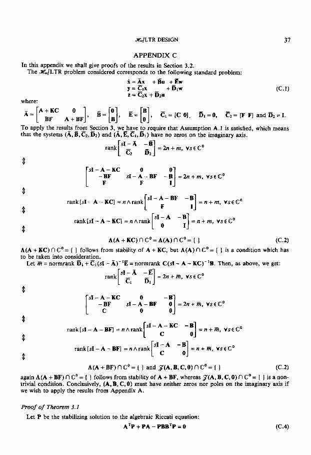
APPENDIX C In this appendix we shall give proofs of the results in Section 3.2.

The %/LTR problem considered corresponds to the following standard problem: X = & +Bu +-Ew Y = C_lX + Dlw (C.1) 2 = czx + Bzu

where: A + K C 0 A = [ BF A+BF] , B = E]. E = c], C I = [C 01, & = O , Cz= [F F] and 6 2 = I .

To apply the results fros ection 3 , _we-ha_ve to require that Assumption A.l is satisfied, which means that the systems (A, B, CZ, Dz) and (A, E, CI, DI) have no zeros on the imaginary axis.

- rank[ SI C~ - A 3 = 2 n + r n , V s € C o

0 -BF s I - A - B F = 2 n + m , VSCC' r-:-, F

8

8

8

rank [sI - A - KC] = n A rank y - y -"I = n + r n , VS€CO I

rank [sI - A - KC] = n A rank

A(A+KC)f lCo=A(A)nCo= [ ] (C.2) A(A + KC) f l Co = to be taken into consi_deratip.

] follows from stability of A + KC, but A(A) n Co = [ ] is a condition which has

Let % = normrank D1 + Cl(sI - A)-% = normrank C(s1- A - KC)-'B. Then, as above, we get:

rank[SIiIA = 2n + T f , Vs € Co

r-:-Kc -B1 0

0

0

$

-BF s I - A - B F 0 = 2 n + R , VsfC'

[,-:-KC -B] = n + f t , VsECo 8

8

8

rank [sI - A - BF] = n A rank 0

rank [sI - A - BF] = n A rank [,,A -3 = n + T f , V S € C O

A ( A + B F ) n C o = ( J and g(A,B,C,O)nCO= ( 1 (C.2) again A(A + BF) f l Co = [ J follows from stability of A + BF, whereas $'(A, B, C, 0) f l Co = [ I is a non- trivial condition. Conclusively, (A,B,C,O) must have neither zeros nor poles on the imaginary axis if we wish to apply the results from Appendix A.

Proof of Theorem 3.1 Let P be the stabilizing solution to the algebraic Riccati equation:

A'P + PA - PBBTP = 0

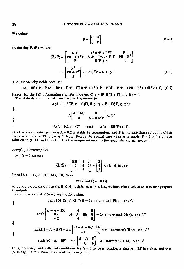
38 J. STOUSTRUP AND H. H. NIEMANN

We define:

- - Evaluating Fy(P) we get:

I

F ~ B ~ P + F ~ F AJP + PAF + F ~ F PB + F~

B'P + F

= PB+F' x [F B T P + F I] 2 0 [ : I (C.6)

The last identity holds because: (A + BF)TP + P(A + BF) + FTF = PBBTP + FTBTP + PBF + FTF = (PB + FT) x (BTP + F) (C.7)

Hence, for the full information transform we get C2.p = [F BTP + FJ and Dp = I. The stability condition of Corollary A.3 amounts to:

A(A + y-*EETP - B(614)-'(BTF + 6TC2)) C C-

A + K C O ] c c -

A[ o A-BBTP

8

8 A(A + KC) c C- and A(A - BBTP) c C-

which is always satisfied, since A + KC is stable by assumption, and P is the stabilizing solution, which exists according to Theorem-A.5. Note, that in the special case when A is stable, P = 0 is the unique solution to (C.4), and thus P = 0 is the unique solution to the quadratic matrix inequality.

Proof of Corollary 3.3

For = 0 we get:

Since H(s) = C(s1- A - KC)-'B, from rank cy(%?) = H(s)

we obtain the condition that (A, B, C, 0) is right invertible, i.e., we have effectively at least as many inputs as outputs.

From Theorem A.2(6) we get the following. - -

rank [By@, s) Gy(Y)] = 2n + normrank H(s), vs c c+ # SI - A - KC 0

-C 0 rank[ BF = 2n + normrank H(s). vsc C'

L

f = n + normrank H(s), vsc c'

0 1 rank[sI - A - BF] = n A

rank[sI-A-BF] = n ~ p--t = n + normrank H(s), VSE c' ~ -

Thus, necessary and sufficient conditions for P = 0 to be a solution is that A + BF is stable, and that (A, B, C, 0) is minimum phase and right-invertible.

&/LTR DESIGN 39

Proof of Theorem 3.5

for the two systems in Figure 4. Utilizing: Theorem 3.5 is proved by showing that the closed loop transfer functions between w to z is the same

Es(s) = STFL(S)MI(S) and

E h ) = STFL(S)M:(S) it is seen, that it suffices to prove that MI@) = M:(s)

MI@) = Ti(s) + Q(s)Tz(s) = F(sI - A - KC)-'B + Q(s)C(SI - A - KC)-'B =F(SI-A-KC)-]B

+ [F(d - A - KC - MIC)-'MI + (BTP + F)(sI - A + BB'P)-'MzC(sI - A - KC - MiC)-'Mi + (BTP + F)(sI - A + BBTP) -*M~]C(~I - A - KC)-'B

+ BTP(sI - A + BBTP)-'M2C(I + (sI - A - KC - MIC)-'MIC)(SI - A - KC)-'B = F(I + (SI - A + BB~P)-~M~c)( I + (SI - A - KC - M~C)-'M~C)(SI - A - KC)-'B

= [F(I + (sI - A + BBTP)-'M2C) + BTP(sI - A + BBTP)-'MzC](~I - A - KC - MiC)-'B = F(s1- A - (K + M')C)-'B + (F + BTP)(sI - A + BBTP)-'M2C(sI - A - (K + Mi)C)-'B

= M ~ ( s ) = T ~ ( s ) + Q*(s)T:(s)

APPENDIX D

Proof of Theorem 3.7 Let P be the stabilizing solution to the algebraic Riccati equation:

ATP + PA - PBBTP = 0

We define P -P

P=[ -P P]

The associated quadratic matrix becomes:

I

(D.4)

PB 1 ATP + PA - A ~ P - PA- PBF F7(F)= -ATP-FTBTP-PA A T P + F T B T P + P A + P B F + F T F -PB-FT [ BTP - B ~ P - F

[ BTP -B'P - F pB I 1 P B B ~ P - PBBTP - PBF = - PBB'P - F ~ B ~ P P B B ~ P + PBF + F ~ B ~ P + F ~ F - PB - F'

= P B + F T x [-BTP B T P + F -I] [ ] The Riccati equation (D. 1) has been exploited to obtain (D.4).

The stability condition of Corollary A.3 amounts to: A(A + y-%ETP - B(nz&-'(BTF+ bTC2)) C 43-

8 h

A-BB'P B ( F - B ~ P ) A + B F

A(A + BF) c C- and A(A - BBTP) c C-

40 J. STOUSTRUP AND H. H. NIEMANN

which is always satisfied, since A + BF is stable by assumption, and P is the stabilizing solution to (D. l), which exists according to Theorem A.2. Note, that in the special case when A is stable, P = 0 is the unique solution to (D. l), and consequently P = 0 is the unique solution to the quadratic matrix inequality.

Proof of Lemma 3.11

Let the observer gain M be given by:

where N satisfies A(A + NC) E 43-. Then N stabilizes A + ME1 since:

] +A(A+NC)tl!A(A+BF)EC- A + N C NC A + B F

A(A + ME') = A

and both A + NC and A + BF are stable by definition. For the norm bound in (73) we have:

( 1 G,P(SI - AP,Q - MG)-'EP,Q IIm

-NC s I -A-BF SI - A - NC

= 11 [ -BTP BTP + F]

= 11 (-B'P + (B'P + F)(SI - A - BF)-'(SI - A))(SI - A - NC)-'B 11- = (1 (F + (B'P + F)(sI - A - BF)-'BF)(sI - A - NC)-'B 11-

(D.7)

Hence, if:

where:

4 = 7/11 F + (B'P + F)(d - A - BF)-'BF )Im (D.lO)

(D.ll)

The existence of N satisfying (D.9) is guaranteed by the hypothesis %? = 0, since it is easily seen that this implies that (A, B, C, 0) is a minimum phase system, i.e. that the i%f& norm of (sI - A - NC)-'B can be made arbitrarily small.

The 2nth-order controller Q ( s ) in (74) with M = [N' NTIT becomes:

SI - A + B B ~ P - NC -BB'P - BF Q(s) = [ -B'P B'P + F] [ -NC $1- A - B F ] [:] (D.12)

By introducing the following similarity transformation of the controller states:

T = [ - I I '1, I T-'=[: ;] (D. 13)

we obtain: S I - A + B B ~ P - N C -BB'P-BF [ -NC SI - A - BF

Q ( s ) = [-B'P BTP+F]T- 'T

sI - A - BF - NC - BB'P - BF ] - ' [i] SI - A + B B ~ P

(D. 14)

= [F BTP + F]

= F(SI - A - BF - NC)-'N

%/LTR DESIGN 41

This is obviously an nth-order controller, actually a standard full-order observer based controller. Applying this controller the sensitivity recovery error becomes:

Es(s) = F(sI - A - BF)-'B - Q(s)[I - C(SI - A)-'BQ(s)] -'C(SI - A)-'B = F(SI - A - BF)-'B - F(SI - A - BF - NC)-'N[I - C ( ~ I - A)-'

X BF(s1- A - BF - NC)-'N] -'C(sI - A)-'B = (I + F(SI - A - BF)-'B)F(SI - A - NC)-'B (D.15)

Since (A, B, C, 0) is minimum phase )I (sI - A - NC)-'B I(- can be made arbitrarily small. Especially we can choose N such that:

)I (sI - A - NC)-'B I(- < y( )I (I + F(s1- A - BF)-'B)F I(oJ)-' (D.16) or

11 Es(.) 11- 6 I( (sI - A - NC)-'B l lw}l (I + F(s1- A - BF)-'B)F 1)- < y (D. 17)

This completes the proof of Lemma 3.11.

APPENDIX E

Proof of Theorem 4.1

We consider the system &,Q described by (78). But first we introduce the following auxiliary system: X = AX + Bu +OW

z = c x + ou

Since this system is stabilizable and detectable, for y sufficiently large the corresponding quadratic matrix inequality has a solution, P. According to Corollary A.4 the quadratic matrix inequality for C* reduced to:

(E.2) A ~ P + PA + C ~ C 2 o

which is independent of 7. Also the associated rank conditions are independent of y:

rank (ATP + PA + CTC) = rank C:,pCz,p = r

and sI-A B

rank[ c2,p = n + r , V S € c'

(E.3)

Hence, the unique solution to the quadratic matrix inequality for all y is the solution to the dissipation inequality for the system C*. (The almost disturbance decoupling problem is solvable for C*, since C* is stabilizable and Im E c Im B). We claim that

- - is a solution to the quadratic matrix inequality for CIO,Q. By evaluating F,(P) we get:

(E.6) 0

F,(P)= 0 ATP+PA+CTC

- - --I 0

For the rank condition (3) in Theorem A.2 we get: rank F,(P) = rank C2.p = r, by (E.3). The other rank

42 J . STOUSTRUP AND H. H. NIEMANN

condition, Theorem A.2(5), amounts to: sI - K rank[ ~ z 2 . p ?] = n + normrank G , VSC c'

SI - A - KC 0 rank [ - B = 2n + normrank(C(s1- A - BF)- 'B), vs C c'

0 C2.P A F

4 rank [sI - A - KC] + rank [" -:,; BF -*] = 2n + normrank(C(s1- A - BF)-'B), Vs 6 c'

0

rank [sI - A - KC] = n A rank iB] = n + r , vs c C+ V

which follows by (E.4) and stability of A + KC.

Proof of Lemma 4.5 Consider the system:

X = (A + BF + Y-~YZ~CI,PCZ.~)X + BU CZ,P x + ou CP,Q:

The system CP,Q is minimum phase" since:

rank [ SI - A - BF - ~-2YzzCT,~Cz,p -"I =rank[ski,pA -9 =#+rank CZ,P V s f C' (E.9) C2.P 0

where the last identity holds according to (81).

A + BF + Y-~YZZC~,PCZ,P + BL is stable, and Thus, by the minimum phase property," ve>O there exists an L such that

11 CZ.P(SI - A - BF - y-2YzzCl,pCz.~ - BL)-' 11 c E

Now substituting LI = - F in: SI - A - KC - BF - BLi

- Y-zYlzcF,Pcz.P SI - A - BF - Y-~YZZCZ,PC~,P - BLz

(E.9)

(E. 10)

we obtain:

(E.ll) The X, norm of this expression can be made arbitrarily small, i.e., especially smaller than 7/(3 - 11 EP.Q 11 ), hence satisfying (A.12) and eventually proving Lemma 4.5.

I -' SI - A - KC - r-2Y IZCF,PCZ.P SI - A - BF - y-2Y2zCI,~C2,~ - BLz

= CZ.P(SI - A - BF - ~-~YzzCT,pCz,p - BL2)-'

Proof of Theorem 4.6

The controller obtained in Lemma 4.5 was; sI- A - KC - MiC ] -' x "1 - Y -zY1zcT,Pcz,P [ -MzC SI - A - BF - Y-~YZZC:,PCZ,P - BLz M2

Q@)= [F - 4 1 x

(E.12)

%/LTR DESIGN 43

where

~ I I = ( S I - A - K C - M ~ C ) - ~ +y-Z(~I-A-KC-M~C)-1Y~~C~,pC~.~A-1M~C(~I-A-KC-M~C)-1 d12 = ~ - ' ( s I - A - KC - MIC)-'Y~ZC;,PCZ,PA-'

= A-'M~C(SI - A - KC - M~C)-' dzz = A-' = (sI - A - BF - y-2YzzC:.p - BLz - y-'MZC(~I - A - KC - M ~ c ) - ~ Y ~ ~ c ; , ~ c ~ , ~ ) - ~

with: = * + ~~z~MzC(~~2Y~zCF.~Cz.p9M~C - (sI - A - KC - M 1c))- 1Y12c:.Pc2.P*

9 = (sI - A - BF - y-2YzzC:,pC2,p - BL2)-' In this notation we have

Q(s) = FdllMl+ Fd~zMz - LzdziMi - LzdzzMz Using this we obtain the following expression for MI: MI(s) = F ~ K B + Q(s)CQKB

=F*KB + FdiiMiC9~B + F ~ ~ z M z C ~ K B - LzdzIMlC+KB - L z ~ z z M ~ C ~ K B = [F + F(s1- A - KC - MIC)-'MIC

+ y-'F(sI - A - KC - MIC)-~Y~ZC;,PCZ,PA-'M*C(~I - A - KC - MIC)-'MIC + y-'F(sI - A - KC - MIC)-~YIZC:,~CZ.PA-~MZC - LzA-'M~C(SI - A - KC - MlC)-'MiC - LZA-~MZCICPKB

= (F + y-'F(sI - A - KC - MIC)-~YIZC:,~C~.PA-~MZC - LzA-'MzC)

= (F + y-'F(sI - A - KC - M~C)-'Y~ZCT,PCZ,PA-~MZC - LzA-'MzC)(sI -A - KC - MIC)-'B = F(sI - A - KC - MlC)-'B + y-'F(sI - A - KC - MIC)-'YIZC:,PCZ.PA-'M~C

X (I + (sI - A - KC - MIC)-lMIC)*KB

x (sI - A - KC - MlC)-'B - LzA-'M2C(sI - A - KC - MIC)-'B = Fdl1B - L~dz1B

= [F - L2] x [ dll d12] x [ 9 d21 dzz SI - A - KC - M1C

-MzC lxE1 - y-2Y1zc:,Pcz,P [ SI - A - BF - y-zYzzC;,pCz,p - BL2 = [F -Lz] X

From this recovery matrix, we can immediately write down the parameters listed in Theorem 4.6.

APPENDIX F

Proof of Theorem 4.7

(A, B, CZJ, 0) is a minimum phase system (see Appendix E). Let P be the unique matrix satisfying ATP + PA + C'C = C:,pCz,p, with rank CZ,P = r, and further that

We claim that - P - P p = [ - P PI

is the solution to the quadratic matrix inequality associated with C1o,st given by (90). Indeed, by substituting this P, F,F) becomes:

ATP+PA+CTC -ATP-PA-CTC O] [ C:p] F,(P) = - ATP - PA - CTC ATP + PA + CTC 0 = - C;,P [CZ,P - CZ.P 01 (F.2) - - [ 0 0 0

which is obviously positive semi-definite. Moreover, we have: - -

rank F,(P) = rank [C2.p - C Z , ~ ] = rank C2.p = r (F.3)

44 J. STOUSTRUP AND H. H. NIEMANN

and

rank ['I-' - "1 =rank[.;. s I - ~ A F !] =rank[ s I -A~] +rank F#) 0 C2,P -C2,p 0

Since P does not depend on y, neither do F.

Proof of Lemma 4.10

First we choose L = [Ll Lz] = F 01 which satisfies (A.12), since then:

sI-A-BF sI- A - BLI

= 1) -C(SI - A - BL&' - C(SI - A - BLI)-'BLz(sI - A - BF)-' + C(SI - A - BF)-' llrn = 0 (F.5) and

-BL2 ] =A(A+BF)kJA(A+BF)cC- SI - A - BF

Hence L = [F 01 is an admissible choice. We shall show that the gain M can be chosen as:

M = [:I where N satisfies A(A + NC) E C, and hence also stabilizes A + MC1:

] =A(A+NC)kJA(A+BF)cQ=- 0 A + B F

a(A + MG) = A

(F.7)

For the left-hand side of the norm bound (A.13) we now have: 11 C~(SI - A - BL)-'BL(sI - A - MCi)-'E 11..

sI-A-NC 0 0 sI-A-BF

c(sI-A)-~B(I-F(sI-A)-~B)-'[F 01 = ll = 11 C(SI - A)-'B(L - F(sI - A)-'B)-'F(sI - A - NC)-'B [Irn = 11 GFL(s)F(sI - A - NC)-'B /Irn < 11 G F L ( ~ ) F )Irn I1 (sI - A - NC)-'B 11- (F.9)

Since (A, B, C, 0) is minimum phase, 11 (sI - A - NC)-'B (Irn can be made arbitrarily small, i.e. we can solve the following optimization problem:

I ( ( ~ 1 - A - NC)-'B IIrn < Y( II GFL(* IF llrn)-l (F. 10) This is guaranteed to satisfy (A.13) by (F.9). The corresponding controller is then given by:

QO)= [F 01 [sI-A-r-NC SI - A O - BF ]-'[:]-=F(sl-A-BF-NC)'N (F.ll)

which is an nth-order controller.

REFERENCES

1. Athans, M., 'A tutorial on the LQG/LTR method', Proc. American Control Conf., Seattle, WA, pp. 1289-12% (1 986).

2. Boyd, S. P., V. Balakrishnan, C. H. Barratt, N. M. Khraishi, X. Li, D. G. Meyer and S . A. Norman, 'A new CAD method and associated architectures for linear controllers', IEEE Trans. Automatic Control, AC-33,

3 . Doyle, J., K. Glover, P. Khargonekar and B. A. Francis, 'State-space solutions to standard M 2 and control

4. Doyle, J., and G. Stein, 'Robustness with observers', IEEE Trans. Automatic Control, AC-24, 607-61 I (1979).

268-283 (1988).

problems', IEEE Trans. Automatic Control, AC-34, 831-847 (1989).

Page number 45 missing