STATE SPACE ANALYSIS AND OPTIMIZATION OF MARX

GENERATOR

BY

NICOLAS NEHME ANTOUN

B.E. Computer Engineering,

Lebanese American University, Lebanon, June 2004

THESIS

Submitted in Partial Fulfillment of the Requirements for the Degree of

Master of Science

Electrical Engineering

The University of New Mexico Albuquerque, New Mexico

July, 2006

© 2006, Nicolas Nehme Antoun

iii

Dedication,

To my dear family

iv

Acknowledgments

I would like to thank my advisor Professor Chaouki Abdallah for his continuous support

through my graduate years as he put his trust in me and gave me the opportunity to

develop both as a student and as a person. I want to express my appreciation to Professor

Peter Dorato who was always available to offer his advice and his perspective of seeing

things which always helped in better understanding the materials in question.

I wan to thank all my dear friends for their continuous support and help.

To my parents, whatever I say or do, I would never be able to express the appreciation

and love I have for you. I want to thank you for everything that you did for me especially

raising me in the best possible way during very hard circumstances.

v

STATE SPACE ANALYSIS AND OPTIMIZATION OF MARX

GENERATOR

BY

NICOLAS NEHME ANTOUN

ABSTRACT OF THESIS

Submitted in Partial Fulfillment of the Requirements for the Degree of

Master of Science

Electrical Engineering

The University of New Mexico Albuquerque, New Mexico

July, 2006

TITLE

STATE SPACE ANALYSIS AND OPTIMIZATION OF MARX GENERATOR

by

Nicolas Nehme Antoun

B.E., Computer Engineering, Lebanese American University, 2004

M.S., Electrical Engineering, University of New Mexico, 2006

ABSTRACT

We introduce in this thesis a set of procedures through which a user is given the ability to

choose a particular desired output behavior from the circuit he is operating and obtain in

return the corresponding set of design parameters that yield the requested output. We will

demonstrate the applicability of these procedures on a Marx generator circuit. We

proceed by introducing a general state space representation algorithm for any stages

Marx generator, then develop a time shifting algorithm that shifts the state trajectories of

the system by the desired amount of time and apply a nonlinear Least-squares

optimization algorithm to determine the set of design parameters.

N

vii

Table of contents

List of Figures x

List of Tables: xiii

Chapter 1 Introduction 1

1.1 Motivation..........................................................................................................1

1.2 Objective ............................................................................................................3

1.3 Methodology ......................................................................................................3

1.4 Conclusions:.......................................................................................................4

Chapter 2 State Space Realization 6

2.1 N-Stages Marx Generator General Characteristics:...........................................6

2.2 N=2-Stage Marx Generator State Space Representation .................................11

2.3 N-Stage Marx Generator general structure state space model.........................19

2.4 Conclusions......................................................................................................22

Chapter 3 System Discretization and Optimization 23

3.1 System discretization .......................................................................................23

3.2 Optimization overview: ...................................................................................24

3.3 Optimization algorithm....................................................................................25

3.3.1 Quasi-Newton Methods:.................................................................... 27

3.3.2 Line Search:....................................................................................... 28

3.3.3 Quasi-Newton Implementation: ........................................................ 29

3.4 Application to the reference model:.................................................................32

viii

3.5 Conclusions......................................................................................................36

Chapter 4 Generating a new reference model 37

4.1 Generating a new reference state model: .........................................................37

4.2 Generating the New Reference Model.............................................................47

4.3 Conclusion: ......................................................................................................49

Chapter 5 Implementation and Results 50

5.1 Case 1: Maximum voltage across fifth capacitor at T= 2.802 seconds ...........50

5.2 Case 2: Maximum voltage across fifth capacitor at T= 3.302 seconds ...........60

5.3 Conclusions:.....................................................................................................69

Chapter 6 Conclusion 71

Appendix A: 74

References: 93

ix

List of Figures

Figure 1 – stages Marx Generator. .................................................................................. 6 N

Figure 2- Generator’s stage discharging process........................................................... 7 thj

Figure 3-1st stage discharge process ................................................................................... 8

Figure 4- A 2-stages Marx Generator ............................................................................... 11

Figure 5- Graph of N=2-stage Marx Generator ................................................................ 12

Figure 6- State trajectory representing the voltage across the parasitic capacitors of a 2-

stage Marx generator................................................................................................. 18

Figure 7- State trajectories obtained using the parasitic capacitor values from the

optimization algorithm.............................................................................................. 33

optX

Figure 8- Relative error between and ................................................................ 34 rX optX

Figure 9- Average error plot between and ........................................................ 35 rX optX .

Figure 10- Voltage across the 5th parasitic capacitor ........................................................ 38

Figure 11- Voltage across the 5th parasitic capacitor up to ....................................... 39 perT

Figure 12- Voltage across the 5th parasitic capacitor up to ft .......................................... 40

Figure 13- Rebuilding up to using symmetry with respect to '5Vc perT ft ......................... 41

Figure 14- Rebuilding up to '5Vc 20totalT = seconds using the periodicity property......... 42

Figure 15- Current across the fifth inductor ..................................................................... 43

Figure 16- Current across the fifth inductor up to .................................................... 44 perT .

Figure 17- Current across the fifth inductor up to ft ....................................................... 45

Figure 18- Rebuilding up to using symmetry with respect to '5Ic perT ft ......................... 46

x

Figure 19- Rebuilding up to '5Ic 20totalT = seconds using the periodicity property ......... 47

Figure 20- New state model ...................................................................................... 51 1nX

Figure 21- Voltage across the fifth parasitic capacitor in lagging the voltage across

the fifth parasitic capacitor in ............................................................................. 52

1nX

rX

Figure 22- State trajectories using the optimal set of parasitic capacitors............... 53 optX

Figure 23- Relative error between and ............................................................. 54 1nX optX

Figure 24- Average error between and ............................................................. 55 1nX optX

Figure 25- Voltage across the first capacitor and the corresponding relative error.......... 57

Figure 26- Voltage across the first capacitor and the corresponding relative error between

for ............................................................................................. 58 .sec16.sec15 ≤≤ T

Figure 27- New state trajectories ............................................................................... 61 2nX

Figure 28- Voltage across the fifth parasitic capacitor in leading the voltage across

the fifth parasitic capacitor in ............................................................................. 62

2nX

rX

Figure 29- State trajectory obtained using the set of optimal parasitic capacitors .. 63 optX

Figure 30- Relative error between and ............................................................ 64 2nX optX .

Figure 31- Average error between and ............................................................ 65 2nX optX

Figure 32- Voltage across the ninth capacitor and the corresponding relative error

between ..................................................................................................................... 66

Figure 33- Voltage across the ninth capacitor and the corresponding relative error

between for .sec12.sec10 ≤≤ T ............................................................................... 67

Figure 34- A N=4-Stage Marx Generator......................................................................... 74

xi

Figure 35- Graph representation of a 4-stage Marx generator.......................................... 75

Figure 36-State trajectory representing the voltage across the parasitic capacitors of a 4-

stage Marx generator................................................................................................. 84

xii

List of Tables:

Table 1- 112M matrix........................................................................................................ 15

Table 2- 122M matrix........................................................................................................ 16

Table 3- 212M matrix........................................................................................................ 16

Table 4- 222M matrix........................................................................................................ 17

Table 5- 114M matrix ........................................................................................................ 80

Table 6- 214M matrix........................................................................................................ 81

Table 7- 124M matrix........................................................................................................ 82

Table 8- 224M matrix........................................................................................................ 82

Table 9- 1111m matrix ......................................................................................................... 86

Table 10- a matrix such that [ ]bam =1211 ..................................................................... 88

Table 11- b matrix such that [ ]bam =1211 ..................................................................... 89

Table 12- 128M matrix ...................................................................................................... 90

Table 13- 1121m matrix ...................................................................................................... 91

Table 14- 1221m matrix...................................................................................................... 92

Table 15- 228M matrix...................................................................................................... 92

xiii

Chapter 1 Introduction

We offer, in this thesis, a circuit operating user with the capability of specifying his

system’s output trajectory and provide him in return with the design parameters whose

output best tracks the desired trajectory or reference model. As an application of this idea

we will use a Marx pulse power generator circuit. Marx generators are based on charging

a number of capacitors in parallel and discharging them in series [1]. Several circuit

representation of a Marx generator exists depending on the manufacturer‘s design and

components used. It was originally described by E. Marx in 1924 and is primarily used

because of its ability to repetitively provide high bursts of voltages especially when the

available voltage sources cannot provide the desired voltage levels [1]. Hence, a voltage

source initially charges the capacitors which are then connected and discharged in series

into the corresponding parasitic capacitors.

1.1 Motivation

The Marx generator is used for a wide range of applications in different research areas

some of which are according to [2]:

Generation of high power microwave using virtual cathode oscillator devices

Lightning testing on cables and insulators.

Material and dielectric testing.

Breaking of raw diamonds in mineralogy.

High voltage and magnetic pulser.

High repetition rate high power CO2 lasers.

1

Generating EMP on parallel plate transmission lines.

Bridge wire exploring.

Electron injection into nuclear reactors.

Electron accelerators.

Kilo amp linear accelerators.

Current injection and generation.

Radiation generation for high voltage steep pulser.

Flash x-ray generation.

Pulsed electron generation.

Short duration luminous flash for ultra high speed photography.

Firing boxes for pyrotechnic substance reliability testing.

Exploding unattended munitions.

Nuclear electromagnetic pulse generator.

Generation of plasma focusing.

Generation of axial plasma for injection purposes.

Remote de-programming of processors used in computers and other control circuitry.

Educational demonstration of electrical pyrotechnics.

However, so far, no one has attempted a state space representation of an stages Marx

generator, and hence no one was able to exploit the simplifications induced by such a

realization to be better design and control the generator. Researchers have attempted to

improve the performance of Marx generators in terms of the electronics and hardware

involved in putting the generator together as was done in [3] and stated in [2]. Hence,

N

2

manufacturers deliver Marx generators with certain specifications and operational

characteristics that the user has to adapt to.

1.2 Objective

The main objective of this thesis is to provide the end user with the ability to specify a

desired behavioral performance from the output of his system, in our case from the Marx

generator he is operating. Consequently, Marx generator models can be standardized, by

providing their users with the ability of specifying the number of stages required for their

application and the instant of time at which the spark should occur. This will eliminate

the need to develop and produce a new generator for each application while freeing the

end user from the constraints involved with some of the manufacturer’s preset

specifications.

1.3 Methodology

To achieve our objective, we decided to first generate an algorithm that determines the

state space model of any stages Marx generator. The next step was to choose a

reference state space trajectory model, so we decided to start from a reference model that

closely approximates the behavior of a Marx generator, but that is by no means ideal.

Now, we want to provide the user with the ability to predefine the time at which the first

spark is to occur. After providing the desired instant of time, we initialize a shifting factor

parameter and develop an algorithm that exploits some of the state trajectory properties to

move the state trajectories by the appropriate amount of time so that the spark occurs at

N

3

the new, user specified time. After obtaining a new state trajectory reference model, we

use a nonlinear least-squares optimization algorithm to determine the values of the design

parameters, in our case the parasitic capacitor values, that best track the reference model.

To show the effectiveness of this technique, we will present a comparison between the

new simulated state trajectories and the corresponding model reference.

Hence, we will start Chapter 2 with the state space realization of an stages Marx

generator and then generalize the results to develop an algorithm that generates the state

space model of for any stages Marx generator. In Chapter 3, we explain the system

discretization process required to successfully apply a nonlinear least-squares algorithm

that we introduce in the same chapter and show its application to a reference state

trajectory model. In the following Chapter 4, we present an algorithm that shifts the

reference state trajectories by a specific shifting factor such that the spark at the

2=N

N

1+N

parasitic capacitor occurs at a user-specified time. In the last chapter, Chapter 5, using

two different shifting factors we apply the state-shifting algorithm of chapter 4 to our

reference model, apply the nonlinear least-squares optimization algorithm to obtain the

corresponding parasitic capacitor values and present the simulation results. Finally, we

conclude this thesis by an overall conclusion summarizing the results that we obtained

and proposing future work and applications.

1.4 Conclusions:

We have described in this chapter how a Marx pulse power generator works and listed

some of the applications for which this generator is used. In addition, we have outlined

4

the procedures that will be used to achieve our objective of providing the users with more

control over their Marx generators.

5

Chapter 2 State Space Realization

We start this chapter by explaining the equations that govern the performance of

any stages Marx generator, then we present an N 2=N stages Marx generator, explain

how it works and derive its corresponding state space model. Extrapolating from the state

space representations of the 2=N stages and 4=N stages (presented in Appendix A)

Marx generators, we develop an algorithm that automatically generates the state space

realization any stages Marx generator. N

2.1 N-Stages Marx Generator General Characteristics:

Figure 1 – stages Marx Generator. N

As explained in Chapter 1, an external voltage source simultaneously charges the

capacitors. After charging these capacitors to the desired initial charge,

the discharging process starts into the corresponding parasitic capacitors through their

respective inductances and load resistances.

1 2 1, , ,NC C C C−L N

For all of the following stages Marx generator models, the load resistances are such

that

N

Ω==== 000,10021 NRRR L , thus the current , for ji Nj ≤≤1 , across the thj

6

resistor will be very small when compared to the corresponding . Hence, we will

assume from now on that the current across the inductor is instead of .

jI

thj jI jj iI −

As a direct consequence of the previous assumption, during the discharging process of

the capacitors, the individual stages can be looked at as: N

The first stage of the circuit

-

Vc1

+

L1

Vc’1+-

I1I2

Figure 2- 1st stage discharge process

the governing voltage law is

21

2

11'1

111

'1

dtVcdLVcVc

dtdILVcVc

+=⇒

−=

7

The remaining stages can be looked at as N

Figure 3- Generator’s stage discharging process thj

By examining Figure 2 we can write any stage voltage equation as: thj

'1

'−+−= j

jjjj Vc

dtdI

LVcVc (1)

where dt

dVcCI jj1−= , hence equation (1) becomes

2' '

12j

j j j j j

d VcVc Vc L C Vc

dt −= + +

Note here that to write the previous two equations we assume the following:

1. at the first stage the stage capacitor discharges into while the next stage

capacitor is not yet connected.

1C '1C

2C

2. For the remaining stages, the parasitic capacitor N '1JC − and discharge into

the corresponding

jC

'JC while the next stages '

1JC +

We now know that at the stage the voltage equation is defined recursively in function

of the previous parasitic capacitors voltages, therefore we can write a general voltage

equation for any of the stages:

thj

N

8

21

2

11121

2

1112

2'

dtVcdCLVc

dtVcd

CLVcdtVcd

CLVcVc jjjj

jjjjj ++++++= −

−−− L (2)

We can simplify the above equation if we have the following assumptions:

LLLL jj ==== − 11 L

CCCC jj ==== − 11 L

Hence, if the previous two constraints are satisfied equation (2) becomes

2 2 21' 1

1 1 2 2 2j j

j j j

d Vc d Vc d VcVc Vc Vc Vc LCdt dt dt

−−

⎛ ⎞= + + + + + + +⎜ ⎟⎜ ⎟

⎝ ⎠L L (3)

Writing the voltage equation at the 1+N parasitic capacitor, we obtain

2 ''' 1

1 11 2

2 '' ' 1

1 1 1 2

NN N NN

NN N N N

d VcVc L CVcdtd VcVc Vc L C

dt

++ ++

++ + +

= −

⇒ = +

(4)

If we replace by in equation (3), we obtain the following equality j N

2 2 2' 1 1

1 1 2 2N N

N N Nd Vc d Vc d VcVc Vc Vc Vc LC

dt dt dt−

−

⎛ ⎞= + + + + + + +⎜ ⎟

⎝ ⎠L L 2 (5)

If we examine equations (4) and (5) in more details we notice that to have a consistent

expression for the resonant frequency at the 1stN + stage, the following equality should

be satisfied

1 1N NL C LC+ + = (6)

When equality (6) is verified, the resonant radiant frequency of the stage capacitors

and the

N

1stN + parasitic capacitor can be expressed by:

LC1

0=ω

9

Using the concept of conservation of energy, we know that all the initial energy stored in

the capacitors must be recovered at the stage, i.e. at . Hence,

knowing that the energy across a capacitor is

NCCC ,,, 21 L thN 1+ 1+NC

2

21 CVcE = , if all the currents and voltages

across stage capacitors are zeros at ft then the following equality must hold

∑=++

N

jjfNN VcCtVcC1

22'1

'1 )0(

21)(

21 (7)

Where represents the initial voltage to which the corresponding capacitor was

charged and is the total voltage discharged into the

)0(jVc thj

)('1 fN tVc + 1+N parasitic capacitor.

Knowing that CCCC NN ==== − 11 L and 011 VVcVcVc NN ==== − L , the above

equation (7) becomes

20

2'1

'1 2

)(21 CVNtVcC fNN =++ (8)

the time ft is such that

0

12ft

f= ,

where 0 0 012

2f f

LCπ ω

π= ⇒ = .

The objective of Marx generators is to have , hence equation (8) becomes 0'

1 )( NVtVc fN =+

20

20

2'1 22

1 CVNVNCN =+

this can only be achieved if

CNCN ⋅=+'

1

this in turn, according to equation (6), implies that

10

NLLN =+1

Note that these results are true for all the stages involved in any stages Marx generator. N

2.2 N=2-Stage Marx Generator State Space

Representation

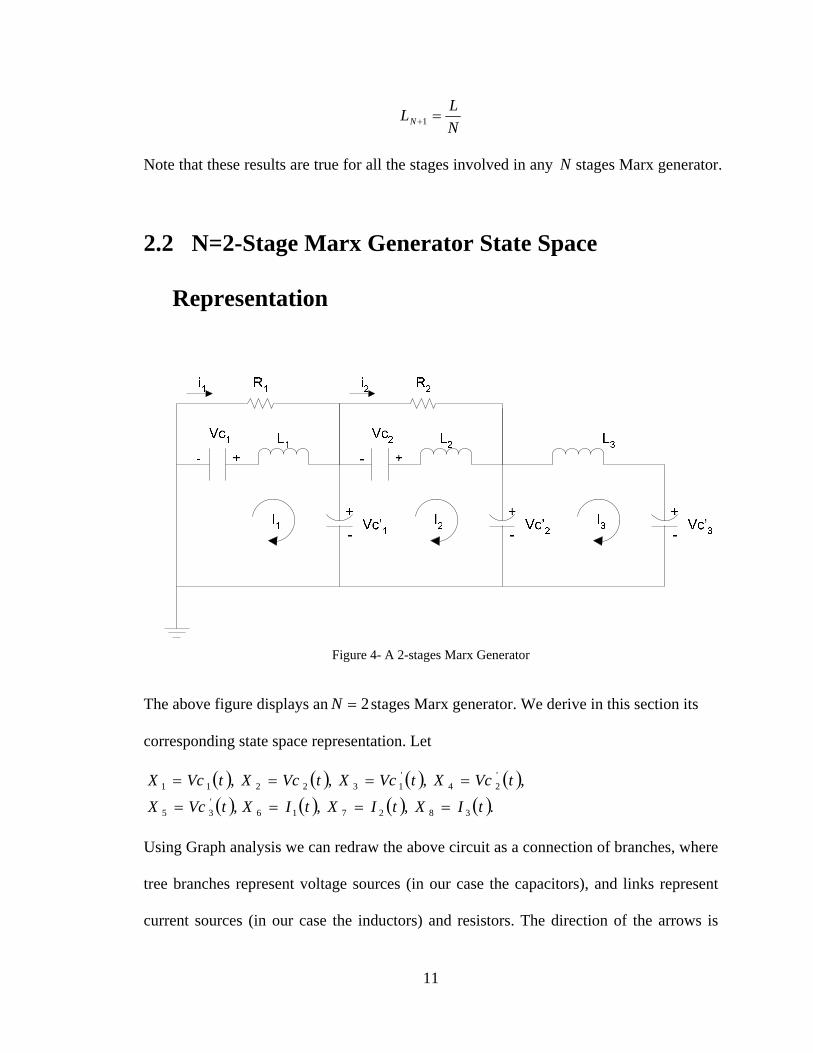
Figure 4- A 2-stages Marx Generator

The above figure displays an 2=N stages Marx generator. We derive in this section its

corresponding state space representation. Let

( ) ( ) ( ) ( )( ) ( ) ( ) ( ).,,,

,,,,

382716'35

'24

'132211

tIXtIXtIXtVcX

tVcXtVcXtVcXtVcX

====

====

Using Graph analysis we can redraw the above circuit as a connection of branches, where

tree branches represent voltage sources (in our case the capacitors), and links represent

current sources (in our case the inductors) and resistors. The direction of the arrows is

11

along the voltage drop in the case of a voltage source, or along the current in the case of a

current source [4]. The corresponding graph representation is therefore:

Figure 5- Graph of N=2-stage Marx Generator

Having chosen the states to be voltages across capacitors and currents across inductors

we follow these two simple rules stated in [4]:

1. Write KCL for every fundamental cut set (i.e. one tree branch and a number of

links) in the network formed by each capacitor in the tree.

2. Write KVL for every fundamental loop (i.e. one link and a number of tree

branches) in the network formed by each inductor in the co-tree (complement of a

tree).

Cut set C1: 11 1 1 1 1 1 60 0dVcC i I C X i X

dt+ + = ⇒ + + =& (9)

Cut set C2: '

' '11 1 1 2 2 1 6 1 3 2 70 0dVci I C i I i X C X i X

dt− − + + + = ⇒ − − + + + =& (10)

12

Cut set C3: ⇒=+⇒=+ 00 72222

2 XXCIdt

dVcC &2 7

2

1X XC

= −& (11)

Cut set C4: '

' '22 2 2 3 2 7 2 4 80 0dVci I C I i X C X X

dt− − + + = ⇒ − − + + =& (12)

Cut set C5: ⇒=−⇒=− 00 85'33

'3'

3 XXCIdt

dVcC &

5 8'3

1X XC

= −& (13)

Loop 1 ( ): 1'11 VcVcI →→

⇒=−+⇒=−+ 00 13611'1

11 XXXLVcVc

dtdIL &

6 11 1

1 13X X

L L= −& X (14)

Loop 2 ( ): 2'1

'22 VcVcVcI →→→

⇒=−−+⇒=−−+ 00 234722'1

'2

22 XXXXLVcVcVc

dtdIL &

7 2 3 42 2 2

1 1 1X X X XL L L

= + −& (15)

Loop 3 ( ): '2

'33 VcVcI →→

⇒=−+⇒=−+ 00 4583'2

'3

33 XXXLVcVc

dtdI

L &8 4

3 3

1 15X X

L L= −& X (16)

Eliminating :, 21 ii

Loop 6 ( ): 1'11 VcVci →→

'1 1 1 1 1 1 3 1 1 1 3

1

10 0 ( )R i Vc Vc R i X X i X XR

+ − = ⇒ + − = ⇒ = − (17)

Loop 7 ( ): '1

'22 VcVci →→

' '2 2 2 1 2 2 4 3 2 3 4

2

10 0 ( )R i Vc Vc R i X X i X XR

+ − = ⇒ + − = ⇒ = − (18)

13

Replacing (17) in (9) we obtain:

⇒=+−+ 01163

11

111 XX

RX

RXC &

1 1 31 1 1 1 1

1 1 16X X X

R C R C C= − + −& X (9)

Replacing (17) and (18) in (11) we obtain:

011

01111

3'

17642

321

211

1

742

32

3'

1631

11

=++−−+

+−⇒

=+−++−+−

XCXXXR

XRR

RRXR

XXR

XR

XCXXR

XR

&

&

1 23 1 3 4 6' ' ' '

1 1 1 2 1 2 1 1 1

1 1 1R R7'

1X X X X XR C R R C R C C C

+= − + + −& X (11)

Replacing (18) in (12) we obtain:

⇒=+++−− 011

4'284

23

27 XCXX

RX

RX &

4 3 4 7' ' '2 2 2 2 2 2

1 1 1 18'X X X X

R C R C C C= − + −& X (12)

Now we have the following set of equations that best describe the state space model of an

N=2-stage Marx generator:

1 1 31 1 1 1 1

1 1 16X X X

R C R C C= − + −& X (9)

2 72

1X XC

= −& (10)

1 23 1 3 4 6' ' ' '

1 1 1 2 1 2 1 1 1

1 1 1R R7'

1X X X X XR C R R C R C C C

+= − + + −& X (11)

4 3 4 7' ' '2 2 2 2 2 2

1 1 1 18'X X X X

R C R C C C= − + −& X (12)

14

5 8'3

1X XC

= −& (13)

6 11 1

1 13X X

L L= −& X (14)

7 2 32 2 2

1 1 14X X X

L L L= + −& X (15)

8 43 3

1 15X X

L L= −& X (16)

Hence, we can now write our state space representation in the following form:

XMX ⋅=2& ,

Where is an ⎥⎥⎦

⎤

⎢⎢⎣

⎡=

222

212

122

112

2

MM

MMM 88× matrix and X is a 1x8 column vector.

112M is a matrix with the following structure: 55×

11

1CR

− 0

11

1CR

0 0

0 0 0 0 0

'11

1CR

− 0 '121

21

CRRRR +

− '12

1CR

0

0 0 '22

1CR

'22

1CR

− 0

0 0 0 0 0

Table 1- matrix 112M

122M is a matrix with the following structure: 35×

15

1

1C

− 0 0

0

2

1C

− 0

'1

1C

'1

1C

− 0

0 '2

1C

'2

1C

−

0 0 '3

1C

Table 2- matrix 122M

212M is a matrix with the following structure: 53×

1

1L

0

1

1L

− 0 0

0

2

1L

2

1L

2

1L

− 0

0 0 0

3

1L

3

1L

−

Table 3- matrix 212M

16

222M is a matrix with the following structure: 33×

0 0 0

0 0 0

0 0 0

Table 4- matrix 222M

Please note for this stages Marx generator structure the following parameters were

used:

2N =

1 2 1FC C C= = = ,

1 2 1HL L L= = = ,

1 2 100 KR R R= = = Ω ,

3 2 1 2H,L N L= × = × =

' '1 20.1578005F, 0.28165FC C= = ,

'5

1 F2

CCN

= =

with resonant frequency, 01 1rad / secLC

ω = = .

During the simulation of this system we initially set 1,2,3 0AI = , and

V, which represents the initial voltage to which the and capacitors were

charged. The following graph represents the voltage trajectories across the parasitic

capacitors:

,1,2,3 0VVc =

12,1 =Vc 1C 2C

17

Figure 6- State trajectory representing the voltage across the parasitic capacitors of a 2-stage Marx generator

Clearly when looking at Figure 6 one can notice that when the voltage across the first two

parasitic capacitors is zero the voltage across the third parasitic capacitor

, where '3 1,2( ) (0) 2 1 2VfVc t N Vc= ⋅ = ⋅ = 2 2 1 3.142

2 2fLCt π π π= = = ≈ seconds. Note

here that at ft the currents across the inductors and voltages across the stage capacitors

are also zero.

18

Please refer to Appendix A for the derivation of the state space model of an stages

Marx generator.

4=N

2.3 N-Stage Marx Generator general structure state

space model

Before delving into the development of the algorithm, it is now clear that the number of

states for an N-stage Marx generator is 23 += NS . This formula was deduced from the

fact that for 2 stages the number of states is 8 and for 4 stages the number of states is 14

(as can be seen in Appendix A).

Going from the state space models of 2N = and 4 stages Marx generator we can

generalize and extrapolate the structure of the MN matrix for any number of stages as

follows:

N

MN can be divided into four blocks as follows:

⎥⎥⎦

⎤

⎢⎢⎣

⎡=

2221

1211

MM

MMM

NN

NNN

is a 11MN ( ) ( 1212 )+×+ NN matrix with the following structure

o , where

⎥⎥⎥⎥⎥⎥

⎦

⎤

⎢⎢⎢⎢⎢⎢

⎣

⎡

+++

+

12,121,12

12,11,1

NNN

N

mm

mm

LLL

MM

MM

MM

LLLLL

o 11

,11,11CR

mm N −=−= , .0122,112,1 == +→+−→ NNN mm

19

o 0121,2 =+→→ NNm

o '11

1,11CR

mN =+ , 0123,12,1 == +→++→+ NNNNN mm , '121

211,1 CRR

RRm NN+

−=++ ,

'12

2,11CR

m NN =++ .

o 0122,1, == +→++→+ NiNiNNiN mm , ')1(,1

iiiNiN CR

m =−++ , '1

1,

iii

iiiNiN CRR

RRm+

+++

+−= ,

'1

)1(,1

iiiNiN CR

m+

+++ = , for Ni →= 2 .

o 0121,12 =+→+ NNm

is a matrix with the following structure 12MN ( ) ( 112 +×+ NN )

o

⎥⎥⎥⎥⎥⎥

⎦

⎤

⎢⎢⎢⎢⎢⎢

⎣

⎡

+++

+

1,121,12

1,11,1

NNN

N

mm

mm

LLL

MM

MM

MM

LLLLL

o i

ii Cm 1

, −= , for Ni ≤≤1 and 0, =jim , for ji ≠ such that and

.

Ni ≤≤1

11 +≤≤ Nj

o '1,,1

jiiii C

mm =−= + for NiN 21 ≤≤+ and . Nj →= 1

o and 01,12 =→+ NNm 01,12 =++ NNm .

is an 21MN ( ) ( )121 +×+ NN matrix with the following structure

20

o

⎥⎥⎥⎥⎥⎥

⎦

⎤

⎢⎢⎢⎢⎢⎢

⎣

⎡

+++

+

1,121,12

1,11,1

NNN

N

mm

mm

LLL

MM

MM

MM

LLLLL

o i

ii Lm 1

, = for Ni ≤≤1 and 0, =jim , for ji ≠ such that and

.

Ni ≤≤1

Nj ≤≤1 0,1 =+ jNm for Nj ≤≤1 .

o 1

1,11L

m N =+ and 0,1 =jm for 122 +≤≤+ NjN .

o j

iiii Lmm 1

1,, =−= + for 12 +≤≤ Ni and 11 +→= Nj , for 0, =jim ji ≠

such that 12 +≤≤ Ni and 121 +≤≤+ NjN .

is an matrix with the following structure 22MN ( ) ( 11 +×+ NN )

o , where all entries

⎥⎥⎥⎥⎥⎥

⎦

⎤

⎢⎢⎢⎢⎢⎢

⎣

⎡

+++

+

1,11,1

1,11,1

NNN

N

mm

mm

LLL

MM

MM

MM

LLLLL

0, =jim for all 11 +≤≤ Ni

and 11 +≤≤ Nj .

As a direct application of this algorithm, we present in Appendix A the state space model

of an stages Marx generator. 8=N

21

2.4 Conclusions

This chapter demonstrated the use of graph theory to determine the state space realization

of an 2 stages Marx generator. By carefully inspecting the state space models of an

and stages Marx generators, we developed an algorithm that generates the

state space model of any stages Marx generator. To this extent, we have also included

in Appendix A the state space model of an

=N

2=N 4=N

N

8=N stages Marx generator using the

algorithm of sectionXX.

22

Chapter 3 System Discretization and

Optimization

We start this chapter with the procedures involved in dicretizing the continuous time

model obtained in the previous chapter. Then we explain the least-squares nonlinear

optimization algorithm and use it in conjunction with the generator’s discrete time model

to determine the values of the parasitic capacitors that will best track a reference state

trajectory model. Please note that from now on, we will be using an stages Marx

generator to explain and demonstrate our work and results.

4=N

3.1 System discretization

Using the state space generation algorithm of 6Chapter 2, we can now determine the

matrix MN such that

)()( tXMtX N ⋅=&

In particular for , we will have the following continuous time state space model: 4=N

)()( 4 tXMtX ⋅=&

where M4 , is the matrix presented in Chapter 2, and is a vector

containing 14 states of the

1414× )(tX 114×

4=N stages Marx generator.

The solution to the above equation is given by

)0()exp()( 4 XtMtX ⋅⋅=

Before applying this optimization scheme, the model was discretized using a time step of

0.002=h seconds, such that the discrete time model representation is of the form

23

)0()()()1(

XGkXkXGkX

k ⋅=⇒

⋅=+

where,

( )244 . . .

2!

MhG I Mh H O T= + + + ,

... TOH are the higher order terms that cancel out as the power of increases i.e.

as and

h

0.. →↑ TOHh I is an identity matrix of size equal to the size of the M4 matrix,

that is . 1414×

3.2 Optimization overview:

Optimization is an approach used to determine the optimal value of a set of design

parameters such that it minimizes or maximizes a defined objective function. Additional

constraints could be defined as lower and upper bounds on the parameters and inequality

or equality constraints on functions of the parameters. In the case where the objective

function and the constraint equations are linear functions of the design variables then the

problem can be solved as a Linear Programming problem. On the other hand, Nonlinear

Programming problem, where the objective function and the constraint equations are

nonlinear in the design variables, the solution is obtained using an iterative process

during which a new direction of search is calculated at each of the iterations [5].

After determining the state space model that best describes the N=4 stages Marx

generator, the objective became to find what values of the parasitic capacitors yield the

desired state behavior. Based on our reference model and as a proof of concept, we will

24

try to track the states’ behavior using a nonlinear least-squares optimization algorithm

and show the effectiveness of this approach when used for our application.

3.3 Optimization algorithm

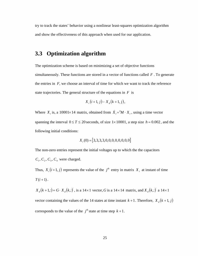
The optimization scheme is based on minimizing a set of objective functions

simultaneously. These functions are stored in a vector of functions called . To generate

the entries in F, we choose an interval of time for which we want to track the reference

state trajectories. The general structure of the equations in is

F

F

( ) ( )jkXjiX dr ,1,1 +−+ ,

Where is, a matrix, obtained from , using a time vector

spanning the interval seconds, of size

rX 1410001× rr XMX ⋅=4&

200 ≤≤ T 100011× , a step size , and the

following initial conditions:

002.0=h

[ ]0,0,0,0,0,0,0,0,3,3,3,3)0( =rX

The non-zero entries represent the initial voltages up to which the the capacitors

were charged. 4321 ,,, CCCC

Thus, represents the value of the entry in matrix at instant of time

.

( jiX r ,1+ )

)

thj rX

)1( +iT

( ) ( ':,:,1 kXGkX dd ⋅=+ , is a 114× vector, is a G 1414× matrix, and a ( )':,kX d 114×

vector containing the values of the 14 states at time instant 1+k . Therefore, ( )jkX d ,1+

corresponds to the value of the state at time step thj 1+k .

25

The algorithm we use is a conjunction of line search procedures and a quasi-Newton

algorithm; the Levenberg-Marquardt method. The function that is minimized is

considered as a sum of squares:

)1()(21)(

21)(min 22

2 ∑==ℜ∈ p

pU

UFUFUfN

where ( ) ( 1, ) ( 1, )p r dF U X i j X k j= + − + .

More accurately, according to [5], we are performing a nonlinear parameter estimation to

fit a model function to data generated in . , has the following structure: rX )(UF

⎥⎥⎥⎥

⎦

⎤

⎢⎢⎢⎢

⎣

⎡

=

)(

)()(

)( 2

1

UF

UFUF

UF

n

M

Please note that in the following, represents the number of stages in the Marx

generator and therefore, for the current case we are studying,

N

4=N . has the

following properties:

)(UF

is an ][ ''2

'1 N

T CCCU LL= N×1 vector containing the values of the design

parameters to be determined.

N

is a )(UJ n N× Jacobian matrix of . )(UF

the gradient vector of . )(UG 1×N )(Uf

the Hessian matrix of . )(UH N N× )(Uf

26

3.3.1 Quasi-Newton Methods:

Quasi-Newton methods are the most popular methods that use gradient information.

These methods formulate the problem as a quadratic problem represented by:

⎟⎠⎞

⎜⎝⎛ ++= bUcUHUUf TT

U 21min)(

where the Hessian matrix, H , is a positive definite symmetric matrix, is a constant

vector, and b is a constant. The optimal solution of this problem occurs when the partial

derivatives of go to zero [5]:

c

)(Uf

0)( =+=∇ ∗∗ cUHUf

Where, according to [6], UHdU

UHUd T

=⎟⎠⎞

⎜⎝⎛

21

, ( ) cdU

Ucd T

= and represents the

optimal solution point.

∗U

The advantage of quasi-Newton methods over Newton methods is the way the Hessian

matrix H is calculated. Newton-type methods calculate H directly and proceed in a

direction of descent to iteratively locate the minimum, which introduces computational

complexities that comes from the numerical generation of H . On the other hand, Quasi-

Newton methods use values of and )(Uf )(Uf∇ to construct curvature information and

generate an approximation of what H should be using the appropriate updating

technique. The most efficient updating method, that proved to guarantee fast convergence

rate and global convergence under the right conditions [13], has been developed by

Broyden [7], Fletcher [8], Goldfarb [9], and Shanno [10], hence its name BFGS:

kkTk

kkTk

Tk

kTk

Tkk

kk sHsHssH

sqqqHH −+=+1

27

where

)()( 1

1

kkk

kkk

UfUfqUUs

∇−∇=−=

+

+

0H , the starting point of the updating technique, can be set to any positive definite

symmetric matrix in particular to the identity matrix. Instead of calculating the inverse of

the Hessian 1−H , the DFP formula, derived by Davidon [11], Fletcher and Powell [12], is

used. The DFP formula uses the same formula as BFGS however while substituting

by :

kq

ks

kkTk

kkTk

Tk

kTk

Tkk

kk qHqHqqH

qsssHH −+= −−

+11

1

Similarly, the gradients of the objective function entries are obtained using a numerical

differentiation method via finite differences based on changing the value of each of the

design parameters and calculating the corresponding rate of change in the objective

function [5].

The direction of search for each iteration can be calculated as follows:

1 ( )k kd H f U−= − ⋅∇ k

3.3.2 Line Search:

Line search is the search method used by the Levenberg-Marquardt algorithm to find the

search direction towards the minimum of the objective function. At each step of the main

algorithm, the line-search method generates a new set of design variables for the next

iteration:

kkk dUU ∗+ += α1

28

where denotes the current iterate, is the search direction and is a scalar step

length parameter.

kU kd ∗α

The line search method attempts to decrease the objective function along the line

by continuously minimizing the objective function. The line search procedure

consists of two phases:

kk dU ∗+α

1. The bracketing phase: corresponding to an interval specifying the range of values

α to be tried-out along the line to be searched such that

.

kkk dUU ∗+ += α1

)()( 1 kk UfUf <+

2. The sectioning phase: dividing the bracket determined in the bracketing phase

into subintervals on which the minimum of the objective function is

approximated by polynomial interpolation.

The resulting step length α satisfies the Wolfe conditions:

( )( ) k

Tkk

Tkk

kT

kkkk

dfcddxf

dfcxfdx

∇≥+∇

∇+≤+

αα

αα

2

1)(

where and are constants with 1c 2c .10 21 <<< cc

These conditions guarantee that we will be using the largest value of α that decreases the

objective function.

3.3.3 Quasi-Newton Implementation:

The quasi-Newton method used consists of two parts:

Determining the direction of search from the updated Hessian matrix using the BFGS

formula;

By looking at the Hessian update formula again:

29

kkTk

kkTk

Tk

kTk

Tkk

kk sHsHssH

sqqqHH −+=+1

where

)()( 1

1

kkk

kkk

UfUfqUUs

∇−∇=−=

+

+

The sign of is dominated by the term : 1+kH kTk sq

( ) ( )( ) ( )( ) ( )kk

Tk

Tkk

Tk

kkkkT

kT

kkTk

kkT

kkkTk

dUfUfsq

UdUUfUfsq

UUUfUfsq

α

α

⋅∇−∇=

−+⋅∇−∇=

−⋅∇−∇=

+

+

++

)()(

)()(

)()(

1

1

11

Knowing that kα is a constant 11× term, we obtain the following expression for : kTk sq

( ) kT

kT

kkkTk dUfUfsq ⋅∇−∇= + )()( 1α

We know that ∑=p

kpk UFUf 2)(21)( , then it is guaranteed that and

. Consequently,

0)( >kUf

0)( >∇ kUf 0)( <− kUf and . From

section XX , hence

0)(0)( <−∇→<∇− Tkk UfUf

)(1kkk xfHd ∇⋅−= − 0<kd :

0)( >∇− kT

k dUf

kT

k dUf )(∇−⇒ α is guaranteed to be positive negative. However, the term

can still be negative. This is where the design of kT

k dUf )( 1+∇−α kα comes into play to

guarantee that is positive definite by guaranteeing: kTk sq

kT

kkT

k

kT

kkT

k

dUfdUf

dUfdUf

)()(

0)()(

1

1

∇−>∇−⇒

>∇−+∇−

+

+

αα

αα

Hence, the Hessian matrix at each iteration is guaranteed to be positive definite so that

the direction of search is always negative and hence in a descent direction. d

30

Consequently, a small step α in the same direction of will decrease the magnitude of

the objective function.

d

The line search procedures;

At each iteration, before a Hessian update is made, the following condition must be

checked:

)()( 1 kk UfUf <+

where dUU kkk α+=+1 .

If does not satisfy the condition above then 1+kU kα is reduced to form a new iteration

step 1+kα . The usual reduction method is a bisection method that involves halving the

current value of α until a reduction in is observed. )(Uf

When a U that satisfies the condition above is found, the Hessian matrix is updated if the

term is positive. If is not positive then further cubic interpolation is performed

such that a valid is found that satisfies the following conditions:

kTk sq k

Tk sq

1kU +

)()( 1 kk UfUf <+

dUf Tk )( 1+∇ is small enough such that 0>k

Tk sq

As approaches the solution point, the procedure goes back to using an kU kα that is close

to unity.

31

3.4 Application to the reference model:

That being said, we applied the nonlinear least-squares optimization algorithm explained

above to the reference state matrix , displayed in Figure 36 of Appendix A. The

results turned out as follows:

rX

0359876.0'1 =C , , , . 06721539.0'

2 =C 02362871.0'3 =C 12467976.0'

4 =C

Looking at the parasitic capacitor values used for the reference model

0359864.0'1 =Cr , , , 067215.0'

2 =Cr 02362875.0'3 =Cr 12467875.0'

4 =Cr

Hence, we have the following differences between the reference model parasitic

capacitors values and the one obtained from the least-squares optimization algorithm:

6'1

'1 102.1 −×−=−CCr , , ,

.

7'2

'2 109.3 −×−=−CCr 8'

3'3 104 −×=−CCr

6'4

'4 1001.1 −×−=−CCr

Which shows that the error between the two sets of parasitic capacitors is relatively small

with an average of 6^1056.2 −×− .

By using the values for the parasitic capacitors obtained from the optimization algorithm

we obtained the following state trajectories stored in : optX

32

Figure 7- State trajectories obtained using the parasitic capacitor values from the optimization algorithm

optX

The relative error between the and , calculated using the following formula: rX optX

),(),(),(

),(jiX

jiXjiXjierr

r

optr −= , for 100011 ≤≤ i and 141 ≤≤ i

Looks as follows:

33

Figure 8- Relative error between and rX optX

Clearly the errors overlap at some of the time intervals. The spikes seen in this graph are

due to the fact that we are plotting the relative error and dividing by which, at

some points in time, when the voltages across the

),( jiXr

51=+N parasitic capacitors are

approaching zero, have very small values that are reflected at spikes in the graph.

For example, the minimum of is , this minimum occurs at index

which corresponds to

)5(:,err 278.6434-

6346=i 69.12)6346( =T seconds. Hence we have

, which corresponds to 6434.278)5,6346( −=err

)5,6346()5,6346()5,6346(

)5,6346(r

optr

XXX

err−

= , where V 007--1.2786e)5,6346( =rX and

34

V 005--3.5755e)5,6346( =optX . We can see that the difference between these two

values is very small and both of them are very close to zero however is of

order and is of order which introduces the spike of

in the relative error plot.

)5,6346(rX

710− )5,6346(optX 510 − 6434.278−

Plotting the average of the error between the two set of states and , we obtain the

following:

rX optX

Figure 9- Average error plot between and rX optX

35

As we can see in the figure, the averages are small having absolute values smaller than

1.1%, more precisely:

1.09%))5(:,( =errmean , %2.0))6(:,( =errmean , 0.0112%))7(:,( =errmean ,

4%-4.8104e))8(:,( =errmean , 0.8729%))9(:,( =errmean .

These results show that the parasitic capacitor values obtained using the least-squares

nonlinear optimization algorithm yield a set of state trajectories that closely follow our

reference model with a relatively negligible error.

3.5 Conclusions

We have seen in this chapter that using the least-squares nonlinear optimization algorithm

yields an optimal set of parasitic capacitor values that, when used for input to the Marx

generator, result in a state model that closely follows the reference model with a

relatively negligible er

rX

ror.

36

Chapter 4 Generating a new reference model

user

4.1 Generating a new reference state model:

It is worth noting that the trajectories of the 14 states have all the following properties:

1. They are periodic with period .

2. Symmetric with respect to, depending on the state in consideration, either their

minimum or maximum value which occurs at

We introduce in this chapter some of the properties associated with the Marx generator

state trajectories and develop a state shifting algorithm that shifts the state trajectories by

a specific shifting factor such that the spark generated by the generator occurs at a

specified time instant.

perT

2per

f

Tt = seconds for each time

interval.

As an illustration of these two properties, consider the voltage across the capacitor,

which corresponds to the 9th state of our model:

perT

1+N

37

Figure 10- Voltage across the 5th parasitic capacitor

Clearly the state trajectory is periodic with period T 6.284= seconds. per

38

perT Figur

The maximum during the first period is 11.9999 at

e 11- Voltage across the 5th parasitic capacitor up to

3.1422per

f

Tt = = seconds,

39

ft Figure 12- Voltage across the 5th parasitic capacitor up to

Having this portion of the state up to t 3.142f = seconds, we can rebuild the state

trajectory for the first period using the symmetrical property with respect to the time

index at which the maximum occurs.

40

e 13- Rebuilding '5Vc up to perT using symmetry with respect to ft Figur

Having rebuilt the data up to the first p full state trajectory can be genera

adding up the rebuilt data for successive multiples of the period up to 20=T seconds

eriod, the ted by

:

41

Figure 14- Rebuilding up to '5Vc 20totalT = seconds using the periodicity property

Having shown the symmetrical and periodical properties of one of the states, in particular

the voltage across the capacitor, we will display one more example of these

properties at the 14th resents the current across the inductor. The

corresponding reference trajectory is displayed in the following figure:

1+N

state which rep 1+N

42

Figure 15- Current across the fifth inductor

Again by looking at Figure 15 we can see that the trajectory is periodic having the same

period as the 9th state, that is 6.284=perT seconds. Displaying the trajectory for the first

period:

43

Figure 16- Current across the fifth inductor up to per

T

T

This trajectory is symmetric with respect to its minimum at 3.1422per

f

3.142ft =

t = = seconds.

Plotting the curve to seconds:

44

Figure 17- Current across the fifth inductor up to ft

Rebuilding the state path up to the first period can be achieved by using the

symmetrical property of the curve with respect to the time index at which the minimum

occurs:

Tper

45

Figure 18 es ect to - Rebuilding 5Ic up to perT using symmetry with r p'ft

The full path can be, hence, built using the peri city of the original curve as is odi

explained for the 9th state trajectory:

46

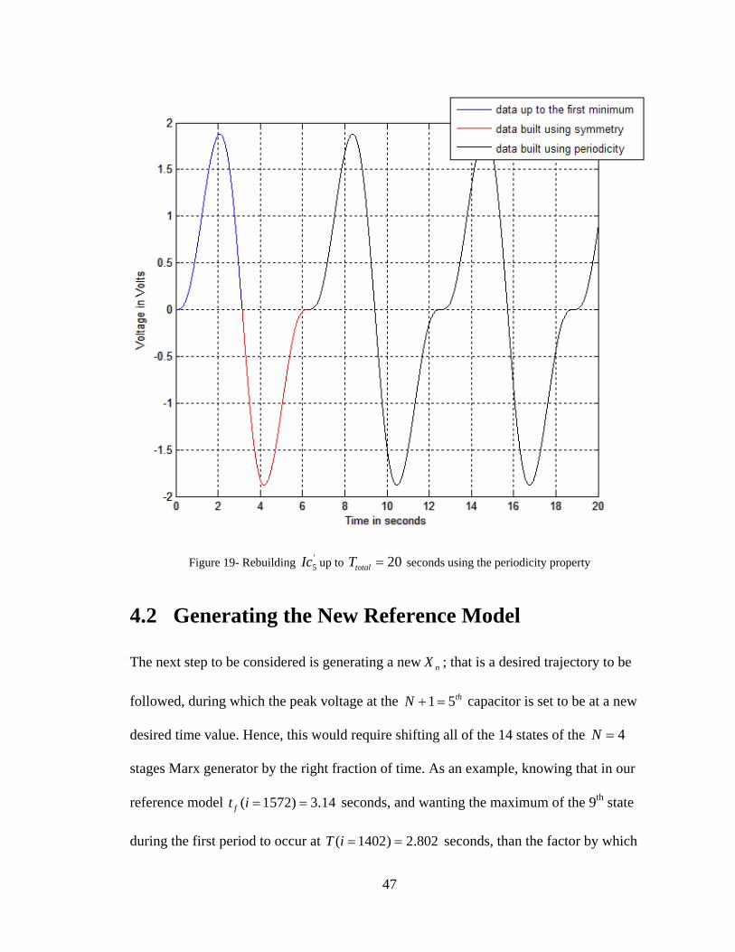
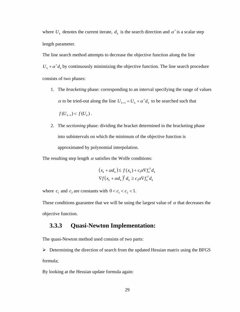
Figure 19- Rebuilding Ic up to ' 20totalT =5 seconds using the periodicity property

4.2 Generating the New Reference Model

The next step to be considered is generating a new ; that is a desired trajectory to be

followed, during which the peak voltage at the capacitor is set to be at a new

desired time value. Hence, this would require shifting all of the 14 states of the

nX

thN 51=+

4=N

stages Marx generator by the right fraction of time. As an example, knowing that in our

reference model seconds, and wanting the maximum of the 9th state ( 1572) 3.14ft i = =

during the first period to occur at 802.2)1402( ==iT seconds, than the factor by which

47

the state trajectories should be shifted by is15721402

=fc

etry

tate shift:

duri

. To this extent and exploiting the

stated state trajectory properties of symm and periodicity, we developed the following

two steps algorithm to reflect the desired s

1st step:

• Define both the maximum and minimum ng the first period and their respective

indices in a variable called temp.

• Define a new array called in which values ranging from 0.01% up to 100%

of the maximum corresponding state variable are stored.

• Go through the entries in and compare them to actual values in in order

to determine their respective indices in . At this stage we consider two scenarios

o The value in is exactly equal to one of the entries of in

this case its entry index would be the same as in

o The value in does not have an exact match in . Therefore it

will eventually be in an interval between a lower and higher bound values

wer

bound entry index of its interval.

The 2nd step:

• We define the shift factor

• We multiply the corresponding maximum value index by , round the result and store

it in

tempXnd _

tempXnd _ dX

dX

tempXnd _ dX

dX .

tempXnd _ dX

in dX . Hence its stored entry index is chosen to be equal to the lo

fc .

fc

inew max__ .

48

• Similarly, we multiply the corresponding value index by fc , round the result

n

minimum

and store it in

• Store at the corresponding maximum value of .

t the corresponding minimum value of

for half a

new period is

inew min__ .

),_max_( jixnewX dX

),min__( jinewX n dX . • Store a

• Move the values stored in tempXnd _ into nX with the corresponding indices being

multiplied by fc .

• Until now we have built nX period, therefore we use the symmetric property

of dX to built nX for a one period duration such that the

min__per ( ) 2)(max__ ×= ineworinewT .

Using the periodicity property of , we fill out the remaining entries of up to •

4.3 Co c

This chapter showed the symmetrical and periodical properties of the states and

presented the algorithm used to generate a new reference trajectory based on these

properties and the reference model , such that the maximum of the parasitic

time.

dX nX

( 10001) 20totalT i = = seconds.

n lusion:

12 +N

nX

rX 1+N

capacitor occurs at a desired point in

49

Chapter 5 Implementation and Results

In this chapter, we apply the state shifting algorithm developed in Chapter 4 to the

reference state model of the 4=N

thN 51 =+

stages Marx generator using two different shifting

nce, we obtain two

tic

squares nonlinear optimization algorithm explained in 23Chapter 3 to obtain the set of

co ari en ults and the

corresponding reference model.

5.1 Case 1: Maximum voltage across fifth capacitor at

T= 2.802 seconds

sing the previous algorithm, we first generated a new where the maximum voltage

tic capacitor occurs at

factors. He new reference state trajectory models with different

voltage peaking times at the parasi capacitor. Next, we apply the least-

parasitic capacitor values that best track the corresponding reference model and present a

mp son betwe the state trajectory obtained using the optimization res

U 1nX

802.2)1402( ==iTacross the thN 51 =+ parasi seconds, i.e.

1572 11402

=fc and .12)9,1402( VX = n

1nX By using the algorithm developed in the previous chapter the new state trajectory

looks as follows:

50

Figure 2 state model

ry. To

will only plot the voltage across the parasitic capacitor in and

:

1nX 0- New

The subsequent figure reflects better the time shift applied to the new state trajecto

avoid confusion, I th9 rX

1nX

51

Figure 21- Voltage across the fifth parasitic capacitor in lagging the voltage across

the fifth parasitic capacitor in

Please note that this same time shift of

1nX

rX

4=N )9(:,1nX

)9(:,rX

340.0802.2142.3)1402()1572( =−=−TT

15721402

=fc is reflected in all of the 14 states of our

stages Marx generator. You can see from the figure that the maximum of

is leading the maximum of our reference model by

seconds.

Using the nonlinear least-squares optimization algorithm, the optimal set of parasitic

capacitor values that best follows the new state trajectories in is the following: 1nX

.F032176.0'1 =C , .F060065.0'

2 =C , .F02111.0'3 =C , .F1115.0'

4 =C

52

Using these values as inputs for the parasitic capacitor values and multiplying

both andC L by to reflect the time shift into the resonant frequencyfc 0ω , we obtain the

following state trajectories stored in : optX

Figure 22- State trajectories optX using the optimal set of parasitic capacitors

53

The states generated using the new set of parasitic capacitors seems to be close

following t tories in 1nX shown in Figure 20. The relative error etween he two

set of state trajectories 1nX and optX

ly

he trajec b

is reflected in the following plots:

Figure 23- Relative error between and

As is reflected in the figure, the spikes of the errors along the different states have larger

magnitudes at certain points in time than the relative error plot shown in Figure 8. The

absolute maximum magnitudes reached by the error between the, new, reference state

trajectories es

1nX optX

1nX and the simulated on optX are as follows:

3005.8))5(:,(max =err , 479.2271))6(:,(max =err , 684.7525))7(:,(max =err ,

1))8(:,(max =err , 142.0193))9(:,(max =err .

54

The next plot shows the mean of the relative error between the states in 1nX gener

using the algorithm in the previous chapter and the ones obtained by simulation using the

optimal set of parasitic acitor d stored in optX :

ated

cap s an

Figure 24- Average error between 1nX and optX

More precis the absolute values of the average percentageely s are:

0.2753%))5(:,( =errmean 12.8018%))6(:,( =errmean 15.9186%))7(:,( =errmean ,

0.5530%))8(:,( =errmean , 2.5711%))9(:,( =errmean .

, ,

55

The above percent averages are small and relatively negligible except for the 6th and 7th

states that have a bit higher average percent error.

If we consider the 5th state more closely, we hav ene se that it has a very large peek of

3005.8, however it has an overall average relative error of 0.2753% which shows that the

peek happens at a fixed instant of time, i.e. at 10.7840)5393( ==iT whereas for the

remaining time indices the corresponding relative error is very small.

It is worth noting that the spikes in the relative error magnitude occur at points in time

where the voltages across the 51=+N parasitic capacitors approach zero volts. Hence,

choosing smaller time intervals during which there are no sudden jumps in the error

magnitude decreases the mean error between any two pair of states significantly.

To better illustrate this statement, the next figure, simultaneously, displays the voltage

across the first parasitic capacitor (i.e. the 5th state in ) and the relative error between

and :

optX

)5(:,1nX )5(:,optX

56

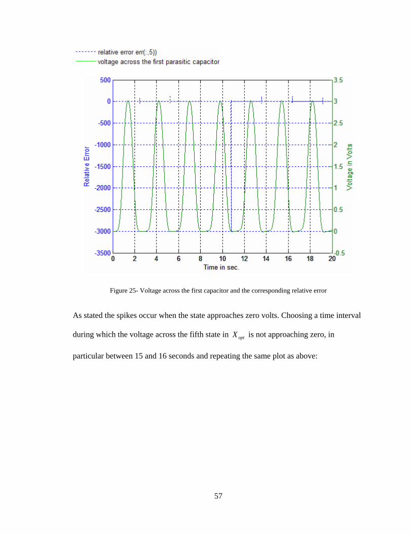
Figure 25- Voltage across the first capacitor and the corresponding relative error

As stated the spikes occur when the state approaches zero volts. Choosing a time interval

during which the voltage across the fifth state in is not approaching zero, in

articular between 15 and 16 seconds and repeating the same plot as above:

optX

p

57

Figu fo

re 26- Voltage across the first capacitor and the corresponding relative error betweenr .sec16.sec15 ≤≤ T

As seen in this figure, the relative error has a small magnitude in this interval:

and absolute mean percentage of:

0.0253 (7501:8001,5) 0.0198err− ≤ ≤

0.0426%))5,8001:7501(( =errmean

Where seconds and 15)7501( =T 16)8001( =T seconds.

The spikes observed in Figure 23 are due to numerical discrepancies induced by the

relative error calculation. For instance, if we again consider in more details the maximum

of the relative error corresponding to the 5th state:

58

8.0053))5(:,(max =err

err matrix, i.e. 8.3005)5,5393( =err . Knowing that This occurs at index 5393 of the

),(),(),(

),(1

1

jiXjiXjiX

jierrn

optn −= , for 100011 ≤≤ i and

Hence,

141 ≤≤ i

)5,5393()5,5393()5,5393(

)5,5393(1

1

n

optn

XXX

err−

=

006-5.8184e)5,

, where

and . Both of these values have

small magnitudes, however one of them e other which induced

the large jump in the relative error magnitude. To overcome this issue, I will set a

threshold value such that whenever the order of is less than while the order

of is less than , set the corresponding relative error value to zero. Hence, with

the application of this constraint, the absolute maximums of the relative state errors

become

5393(1 =nX 2101.75)5,5393( −×=optX

has order 210 − and th 610 −

1nX 310 −

optX 210 −

:

19.3360))5(:,(max =err , 1))6(:,(max =err , 0.9865))7(:,(max =err ,

0.3239))8(:,(max =err 0.9475))9(:,(max =err, .

with the following absolute mean percentages:

2.1227% ))5(:,( =errmean , 3.1654%))6(:,( =errmean , 0.8188%))7(:,( =errmean ,

0.4509%))8(:,( =errmean , 1.3447% ))9(:,( =errmean .

Thus the absolute maximum and percentage average of the relative errors have been

greatly decreased, which shows the effect of calculation discrepancies on the error

especially in regions where the state variable values become minute when approaching

zero.

59

5.2 Case 2: Maximum voltage across fifth capacitor at

The next case considered is when the maximum voltage across the parasitic

capacitor occurs at

T= 3.302 seconds

thN 91=+

3.302 )1652( ==iT seconds, i.e.

.12)9,1652(2 VX n = 15

721652

=fc and

Hence, the new state trajectories look as follow:

60

Figure 27- New state trajectories

he subsequent figure reflects better the time shift applied to the new state trajectory. To

void confusion, I will only plot the voltage across the parasitic capacitor in and

:

2nX

T

a th9 rX

2nX

61

Figure 28- Voltage across the fifth parasitic capacitor in leading the voltage across

the fifth parasitic capacitor in

Please note that this same time shift of

2nX

rX

15721652

=fc

ou can see from

is also reflected in all of the 14 states

of our N=4 stages Marx generator. Y the figure that the maximum of

is lagging the maximum of our reference model by )9(:,2nX )9(:,rX

16.0142.3302.3)1572()1652( =−=−TT seconds.

Again using the nonlinear least-squares optimization algorithm, the optimal set of

parasitic capacitor values that best follows the new state trajectories is the following: 2nX

.F037819.0'1 =C , .F070636.0'

2 =C , .F024877.0'3 =C , .F13122.0'

4 =C

62

Using these values as inputs for the parasitic capacitor values and multiplying

both andC L by to reflect the time shift into the resonant frequencyfc 0ω , we obtain the

following state trajectories stored in : optX

Figure 29- State trajectory optX obtained using the set of optimal parasitic capacitors

From the above plot, the state trajectories seam to follow the new reference mod

much better

el

than the previous case. The resulting relative error plots are as follows:

2nX

63

Figure 30- Relative error between and

Still one can notice the jumps in the magnitude of the relative error that are larger than

the ones shown in Figure 8, however much smaller than the spikes obtained in the

previous study case. The absolute maximums of the relative error magnitudes are as

follows:

2nX optX

258.8794))5(:,(max =err , 2319.9))6(:,(max =err , 558.8778))7(:,(max =err ,

1))8(:,(max =err , 418.3080))9(:,(max =err .

The subsequent plot shows the mean of the relative error between the states in and 2nX

the ones obtained by simulation optX :

64

Figure 31- Average error between 2nX and optX

The absolute values of the averages are:

( (:,5)) 26.6565%mean err = , ( (:,6)) 3.8268%mean err = , ( (:,7)) 1.0534%mean err = ,

( (:,8)) 0.3932%mean err = , ( (:,9)) 0.5068%mean err =

.

eptio of the one corresponding to the 5th state. The large

average error value is due to the larger spikes in the corresponding relative error as

shown in Figure 30.

Similarly to the reasoning behind the first case study, the percentages shown above are

clearly small enough for the exc n

65

Again the spikes in the relative error magnitude occur at points in time where the voltage

across the parasitic capacitors approaches zero volts.

Similarly to the previous case, choosing smaller time intervals during which there are no

sudden jumps in the error magnitude decreases the mean error between any two pair of

states significantly. The following figure, gives a better pictorial explanation of this fact

by simultaneously displaying the voltage across the fifth parasitic capacitor (i.e. the 9th

state in ) and the relative error between and :

1+N

optX )9(:,2nX )9(:,optX

Figure 32- Voltage across the ninth capacitor and the corresponding relative error between

66

As stated the spikes occur when the state approaches zero volts. Choosing a time interval

during which the voltage across the ninth state in optX is not approaching zero, in

particular between 9 and 12 seconds and repeating the same plot as above:

Figure 33- Voltage across the ninth capacitor and the corresponding relative error between for .sec12.sec10 ≤≤ T

As is reflected by the figure above, the relative error of the 9th state has a small

magnitude in this interval:

005--5.51697e6001,9):err(50010.024329- ≤≤ ,

and absolute mean percentage of:

0.50413%))9,6001:5001(( =errmean

67

Where 10)5001( =T seconds and 12)6001( =T seconds.

As stated for the previous study case, the spikes observed in Figure 32 are due to

numerical discrepancy induced by the relative error calculation. For instance, if we

consider the maximum of the relative error corresponding to the 5th state:

258.8794))5(:,(max =err

This occurs at index 6831 of the err matrix, i.e. 8794.258)5,6831( =err . Knowing that

),(),(),(

),(2

2

jiXjiXjiX

jierrn

optn −= , for 100011 ≤≤ i and

Hence,

141 ≤≤ i

)5,6831()5,6831()5,6831(

)5,6831(2

2

n

optn

XXX

err−

=

5

, where

and . Both of these

values have small ma and the other

which induced the large jump in the relative error ma ld value

such that whenever the order of both and is less than or equal to set the

corresponding relative error value to zero. Hence, with the application of this constraint,

the absolute maximums of the relative error become:

2 1027509698.3)5,6831( −×−=nX 3104458.8)5,6831( −×=optX

gnitudes however one of them has order 510 − 310 −

gnitude. By setting a thresho

2nX optX 310 −

0.4166))6(:,

0.0239))8(:,(max =err , 80.756))9(:,(max =err

6.0306))5(:,(x =err , (max =err , 0.058))7(:,(max =errma 2 ,

.

mean percentages: with the following absolute

0.0524%))5(:,( =errmean , 0.0436%))6(:,( =errmean , 0.1377%))7

0.1121% , 4.4930%))9(:,( =errmean .

(:,( =errmean ,

))8(:,( =errmean

68

Again, the absolute maximum and verages h percentage a ave been greatly decreased,

ns

5.3 Conclusions:

The main area of interest in the state trajectories is when the voltage across the

which shows the effect of calculation discrepancies on the error especially in regio

where the state variable values become minute when approaching zero.

1+N

capacitor reaches its maximum of '1N NVc =+ , where )0 Ni ,,

N

nX

de,

a e error value which underm

('iVc⋅ 2,1 L= while the

voltage across the remaining parasitic capacitors is approaching zero. Using the state

space generation algorithm we have explained in Chapter 2 to generate a new desired

state trajectory and the least-square nonlinear optimization algori

ate

tha

tiv ines

the effect of the sudden jumps in the relative error magnitude. It is worth noting here that

the time shift in this section could have been reproduced by time scaling the state space

thm to obtain the

optimal set of parasitic capacitors to track the new nX , we obtained optX whose st

trajectories closely follow the desired nX especially in the interval of interest. Adding a

constraint to the relative error magnitu such t whenever the value of the states go

down below a certain threshold value set the corresponding relative error to zero, proved

that optX closely follows nX with negligible mean rel

model of the Marx generator

1( ) ( )N

i

X t M Xfc

= ⋅& t

It is worth noting here that the time shift in ection could have been y

time scaling the state space model of the Marx generator

this s reproduced b

69

1( ) ( )N

i

X t M X t= ⋅&

However, even though this concept is applicable for the case of a Ma

fc

rx generator it is

annot be generalized for any state space mode. The goal here is to show that by shifting

the state trajectories of a particular system it is still possible to determine the design

e desired output.

c

param ters that will yield the

70

Chapter 6 Conclusion

ze Marx generators with arbitrary large

number of stages and introduces the advantage of knowing the behavior of the voltages

across the capacitors and the currents across the inductors at all instance of time and

hence prevent any unpleasant behavioral surprise.

We developed in Chapter 4 an algorithm that exploits the state trajectory properties of

periodicity and symmetry to construct a new set of states that comply with the user’s

desired specifications. Hence, a user can now specify the time at which he desires the

voltage across the parasitic capacitor to peek, that is the time instant

We demonstrated in this thesis how to generate the appropriate state space model for any

N stages Marx generator by simply following the algorithm developed in Chapter 2. This

state space representation can be used to analy

1+N ft at which

, where ' '1( ) (0)N f iVc t N Vc+ = ⋅ Ni ,,2,1 L= , and the algorithm generates the appropriate

state trajectories that achieve that goal. This is where the application of the nonlinear

least-squares algorithm comes into play. Up till now the new desired state trajectories are

just theoretical and not the resulting output of the corresponding Marx generator. To be

able to determine the parasitic capacitor values that produce the desired state behavior,

we used a nonlinear least-squares optimization algorithm based on the quasi-Newton

Levenberg-Marquardt algorithm with line search procedures.

This strategy was shown to be successful with small relative error between the state

trajectories in , obtained from the new set of parasitic capacitors, and the new

desired trajec , generated using the algorithm of Chapter 2. At some particular

optX

tories in nX

71

instants of time, we encountered large jumps in the relative error magnitude. More

e error peeks occur at instants of time when the voltages across the

parasitic capacitors are approaching zero. These jumps can be undermined without

behavior of a Marx generator using a base

e

voltage across the parasitic capacitor is peeking while the remaining voltages

and currents are app oaching zero. In addition to the numerical discrepancies induced by

the calculation of the relative error, these error magnitude jumps might be due to the

optimization algorithm we are using that has proven to be less efficient when

encounterin inaccuracies. Hence, by setting a threshold value such that

whenever the state value goes below that threshold the error is set to zero, we were able

to eliminate all the spikes and hence obtain both relative error and mean error values that

are negligible. It i g that we gen

tages generator using the

e

are

precisely, the relativ

1+N

any seriou

N 1+

r

g line search

s wo

trajectory models of 1, 2, , 2N N− − L stages Marx generators. Besides that, it would b

interesting to apply the concepts in this thesis to an actual Marx generator and comp

s effect on the system’s behavior; primarily because we are approximating the

reference model that is by no means ideal and

because they do not occur at time intervals of interest that is the time intervals when th

( )st

rth notin erated the new sets of “desired” state

trajectories based on a model that is an approximation of what the behavior of a Marx

generator would be. Therefore, obtaining and basing our new state trajectories on a

reference model that has proven to be more accurate can greatly improve our results as

we will be attempting to track more realistic state trajectory models. Other issues worth

looking at are using another variation of the optimization algorithm such as the Guass-

Newton methods and predicting the state trajectories of an N s

72

the simulation results to the practical results and, thus, obtain a better idea of the acc

and effectiveness of the results obtained in this thesis.

fore by applying the concepts developed in this thesis to a Marx generator circuit,

we have showed that by generating the state space model of any circuit in combination

with the appropriate optimization algorithm, a user can specify a desired output trajectory

of hi circuit at a particular instant of time and determine in return the design parameters

that yield a trajectory that best tracks his output reference model.

As an interesting application of the concepts developed in this thesis, provided

appropriate safety measures are taking into consideration, I propose providing the use

with an interface through which he can specify the instant of time he desires th

the 1N + parasitic capacitor to occur and the number of stages he desires, this numb

would be dependant on the charging voltage sources available for the user and the

maximum output voltage value he is seeking. The device’s memory will contain the state

space trajectories for a wide range of stage numbers. The tool will then use the shif

algorithm of Chapter 4, the state space generation algorithm of Chapter 2 and the

nonlinear least-squares optimization algorithm of Chapter 3 to generate the appropria

parasitic capacitor values that will simulate the state space trajectories that conform to th

user’s specifications.

uracy

There

r

e spark at

er

ting

te

e

73

Appendix A:

A.1 N=4-Stage Marx Generator

Now computing the state space realization of an N=4 stages Marx generator:

Figure 34- A N=4-Stage Marx Generator

Let

( ) ( ) ( ) ( ) ( ) ( )( ) ( ) ( ) ( ) ( )

.,,,,,,

,,,,,,

514413

312211110'59

'48

'37

''

tIXtIXIXtIXtIXtVcXtVcXtVcX

tVcXtVcXtVcXtVcXtVcXtVcX

========

======

Similarly to the 2-stage Marx generator, using graph theory we obtain the following

graph

( )( ) ( )

,261544332211

t

74

Figure 35- Graph representation of a 4-stage Marx generator

Having chosen the states to be voltages across capacitors and currents across inductors

we follow these two simple

. Write KCL for every fundamental cut set (i.e. one tree branch and a number of

links) in the network formed by each capacitor in the tree.

4. Write KVL for every fundamental loop (i.e. one link and a number of tree

branches) in the network formed by each inductor in the co-tree (complement of a

Cut set C1:

rules stated in 93[4]:

3

tree).

11 1 1 1 1 1 100 0dVcC i I C X i X

dt+ + = ⇒ + + =& (A.1.1)

Cut set C2: '

' '11 1 1 2 2 1 10 1 5 2 110 0dVci I C i I i X C X i X

dt− − + + + = ⇒ − − + + + =& (A.1.5)

Cut set C3: ⇒=+⇒=+ 00 112222

2 XXCIdt

dVcC & 2 12

11X X

C= −& (A.1.2)

Cut set C4: '

' '22 2 2 3 3 2 11 2 6 3 120 0dVci I C i I i X C X i X

dt− − + + + = ⇒ − − + + + =& (A.1.6)

75

⇒=+⇒=+ 00 123333

3 XXCIdt

dVcC &

3 13

12X X

C= −&Cut set C5: (A.1.3)

Cut set C6: '

' '33 3 3 4 4 3 12 3 7 4 120 0dVci I C i I i X C X i X

dt− − + + + = ⇒ − − + + + =& (A.1.7)

Cut set C7: ⇒=+⇒=+ 00 134444

4 XXCIdt

dVcC &4 1

4

13X X

C= −& (A.1.4)

Cut set C7: '

' '44 4 4 5 4 13 4 8 140 0dVci I C I i X C X X

dt− − + + = ⇒ − − + + =& (A.1.8)

Cut set C8: ⇒=+−⇒=+− 00 9'514

'5'

55 XCXdt

dVcCI &

9 1'5

14X X

C=& (A.1.9)

Loop 1 ( VcI →→ '11 1Vc ):

⇒=−+⇒=−+ 00 151011'1

11 XXXLVcVcdIL &

10 1 51 1

1 1

X X X= −& (A.1.10) dt L L

Loop 2 ( ' VcVcVcI →→→ ): 2121

⇒=−−+⇒=−−+ 00 2561122'1

'2 XXXXLVcVcVc &

'

11

22 dt

dIL

2 5 62 2 2

1 1 1X X X X= + − (A.1.11)

3I →

L L L&

Loop 3 ( VcVcVc →→ ): 3'2

'3

12 3 6 7

⇒=+ 03'3

33 Vc

dtL −−+⇒=−− 0 671233

'2 XXXXLVcVc

dI &

3 3 3

1 1 1X X X XL L L

= + −& (A.1.12)

Loop 4 ( ): 4'3

'44 VcVcVcI →→→

⇒=−−+⇒=−−+ 00 4781344'3

'4

44 XXXXLVcVcVc

dtdIL &

13 44 4

7 84

1 1 1X XL

=& X XL L

+ − (A.1.13)

76

Loop 5 ( 5I → '4

'5 VcVc → ):

⇒=−+⇒=−+ 00 89145'4

'5

55 XXXLVcVc 14 8 9

5 5

1 1X X XL L

= −&dtdI

L & (A.1.14)

Eliminating

Loop 6 ( ):

:,,, 4321 iiii

1'11 VcVci →→

'1 1 1 1 1 1 5 1 1 1 5

1

10 0 ( )R i Vc Vc+ − R i X X i X XR

= ⇒ + − = ⇒ = − (A.1.15)

VcVc → ): '1

'2Loop 7 ( 2i →

' '2 2 2 21 2 6 5 2 5 6

2

10 0 ( )R i Vc Vc R i X X i X XR

+ − = ⇒ + − = ⇒ = − (A.1.16)

Loop 8 ( ): '2

'33 VcVci →→

' '3 3 3 2 3 3 7 6 3 6 7

3

10 0 ( )R i Vc Vc R i X X i X XR

+ − = ⇒ + − = ⇒ = − (A.1.17)

Loop 9 ( ): '3

'44 VcVci →→

' '4 4 4 3 4 4 8 7X X− = 4 7 8

4

10 0 ( )R i Vc Vc R i i X XR

+ − = ⇒ + ⇒ = − (A.1.18)

(A.1.15) in (A.1.1) we tain: Replacing ob

⇒=+−+ 011105

11

111 XX

RX

RXC &

1 1 51 1 1 1 1

1 1 110X X X

R C R C C= − + −& X (A.1.1)

Replacing (A.1.15) and (A.1.16) in (A.1.5) we obtain:

011

01

1 25 1 5 6' X

R C+ 10 11' ' ' '

1 1 1 2 1 2 1 1 1

1 1 1 1R RX X X X XR C R R C C C

+= − + −& (A.1.5)

111 +− X 1

5'

1111062

521

211

1

1162

52

5'1105

11

=++−−+

+−⇒

=+−+−+

XCXXXR

XRR

RRXR

XXR

XR

XCXXRR

&

&

77

Replacing .1 (A.1.16) and (A .17) in (A.1.6) we obtain:

011

01111

6'212117

36

32

325

2R

1273

63

6'2116

25

2

=++−−+

+−⇒

=+−++−+−

XCXXXR

XRR

RRX

XXR

XR

XCXXR

XR

&

&

2 36 6

15 7 11 12' ' ' ' '

2 2 2 3 2 3 2 2 2

1 1 1R RX X X X X XR C R R C R C C C

++ + − (A.1.6)

Replacing (A.1.17) and (A.1.18) in (A.1.7) we obtain:

= −&

011

01111 '36− CX

R

7'313128

47

43

436

3

1384

74

712733

=++−−+

+−⇒

=+−++−+

XCXXXR

XRR

RRX

R

XXR

XR

XXXR

&

&

3 47 7

16 8 12 13' ' ' ' '

3 3 3 4 3 4 3 3 3

1 1 1R RX X X X X XR C R R C R C C C

+− + − (A.1.7)

Replacing (A.1.18) in (A.1.8) we obtain:

= +&

0118

'414138

47− XX

R4

=++−+ XCXXR

&

8 7 8 13' ' ' '4 4 4 4 4 4

1 1 1 114X X X X

R C R C C C= − + −& X (A.1.8)

ns: Now we have the following set of equatio

101

511

111

1111 XC

XCR

XCR

X −+−=&

112

21 X

CX −=&

123

31 X

CX −=&

134

41 X

CX −=&

78

11'1

10'1

6'12

5'121

21 1111 XXXXRRXX −+++

−=&1'

115 CCCRCRRCR

12'2

11'2

7'23

6'232

325'

226

1111 XC

XC

XCR

XCRRRRX

CRX −++

+−=&

13'3

12'3

8'34

7'343

436'

337

1111 XC

XC

XCR

XCRRRRX

CRX −++

+−=&

14'4

13'4

8'44

7'44

8 XC

XC

XCR

XCR

X −+−= 1111&

14'5

91 X

CX =&

51

11

1011 XL

XL

X −=&

62

52

22

11111 XL

XL

XL

X −+=&

73

63

33

12111 XL

XL

XL

X −+=&

84

74

44

13111 XL

XL

XL

X −+=&

95

85

14 XL

XL

X −=& 11

Hence, we can now write our state space representation of the form:

XMX ⋅=4& ,

Where 4

MM

MMM is a

⎥⎥⎦

⎤

⎢⎢⎣

⎡=

224

214

124

11 1414× matrix and X is a 1x14 column vector. 4

79

114M is a 9x9 matrix and has the following structure

RC1

− 0 0 0 RC1

'1

1RC

'1

)(RRC

RR +− '

1

1RC

'2

1RC

'2

)(RRC

RR +− '

2

1RC

'3

1RC

'3

)(RRC

RR +− '

3

1RC

'4

1RC

'4

1RC

−

0 0 0 0

0

0 0 0 0 0 0 0 0

0 0 0 0 0 0 0 0 0

0 0 0 0 0 0 0 0 0

0 0 0 0 0 0

0 0 0 0 0 0

0 0 0 0 0 0

0 0 0 0 0 0 0

0 0 0 0 0 0 0 0 0

Table 5- matrix 114M

80

214M is a 6x9 matrix and has the following structure:

L1 0 0 0

L1

−

L1

L1

L

L L1

L1

−

L1 0 0

L1

L1

−

5

1L

5

1L

−

0 0 0 0

0 1

1

0

−

0 0 − 0 0 0

0 0 0 0 0 0

0 0 0

0 0 0 0 0 0 0

Table 6- matrix

is a 9x5 matrix and has the following structure:

214M

124M

C1

C1

−

C1

−

C1

− 0

'1

1C

'1

1C

−

'2

1C

'2

1C

− 0 0

0 0 0 0

0 0 0 0

0 0 0 0

0 0 0

0 0 0

0

81

0 0 1 '3

'3

1C

−

'4

1C

'4

1C

−

'5

1C

s to all the constraints fo sta ato

C0

0 0 0

0 0 0 0

Table 7- matrix

is a 5x5 matrix and has the following structure:

0 0 0 0 0

124M

224M

0 0 0 0 0

0 0 0 0 0

0 0 0 0 0

0 0 0 0 0

Table 8- matrix

Please note that the stages Marx generator structure that we are presenting

conform set in Chapter 2 r a general ges Marx gener r and

has, similarly to the stages Marx generator, the following parameter values:

,

,

F

224M

4N =

N

2N =

1 2 3 4 1C C C C C F= = = = = ,

1 2 3 4 1L L L L L H= = = = =

1 2 3 4 100,000R R R R R= = = = = Ω

5 4 1 4L N L H= × = × = ,

' ' ' '1 2 3 40.03599 , 0.067215 , 0.02363 , 0.12468C F C F C F C= = = = ,

82

'5

14

CC FN

= =

The sim were obtained by initially setting ulation results for this system 1,2,3,4,5 (0) 0I A= ,

and ,1,2,3,4,5 (0) 0Vc V= 1,2,3,4 (0) 3Vc V= , which represents the voltage value to which the

capacitors were initially charged: 1 2 3 4, , ,C C C C

83

Figure 36-State trajectory representing the voltage across the parasitic capacitors of a 4-stage Marx generator

Similarly to the N=2-stage Marx generator, at the instant of time seconds, the

voltage across the first four parasitic capacitors, , is approximately zero,

and the voltage across the fifth parasitic capacitor,

3.142ft =

,4

,3

,2

,1 ,,, VcVcVcVc

,5 1,2,3,4( ) (0) 4 3 12 .fVc t N Vc V= ⋅ = ⋅ =

84

A.2 N=8-Stage Marx Generator

Using the algorithm developed in Chapter 2 we can generate the corresponding

M8 matrix for an N=8-stages Marx generator.

First we know that the number of states expected from an N=8 stages Max generator

would be 2628323 =+⋅=+= NS , therefore our matrix would

have to be a

⎥⎥⎦

⎤

⎢⎢⎣

⎡=

228

218

128

118

8

MM

MMM

2626× matrix.

If we start by considering , we know that it will have a size of 118M ( ) ( )1212 +×+ NN ,

that is with the following structure: 1717×

[ ]1211

1111

118 mmM = , where and are respectively 11

11m 1211m 817× and

matrices:

917×

85

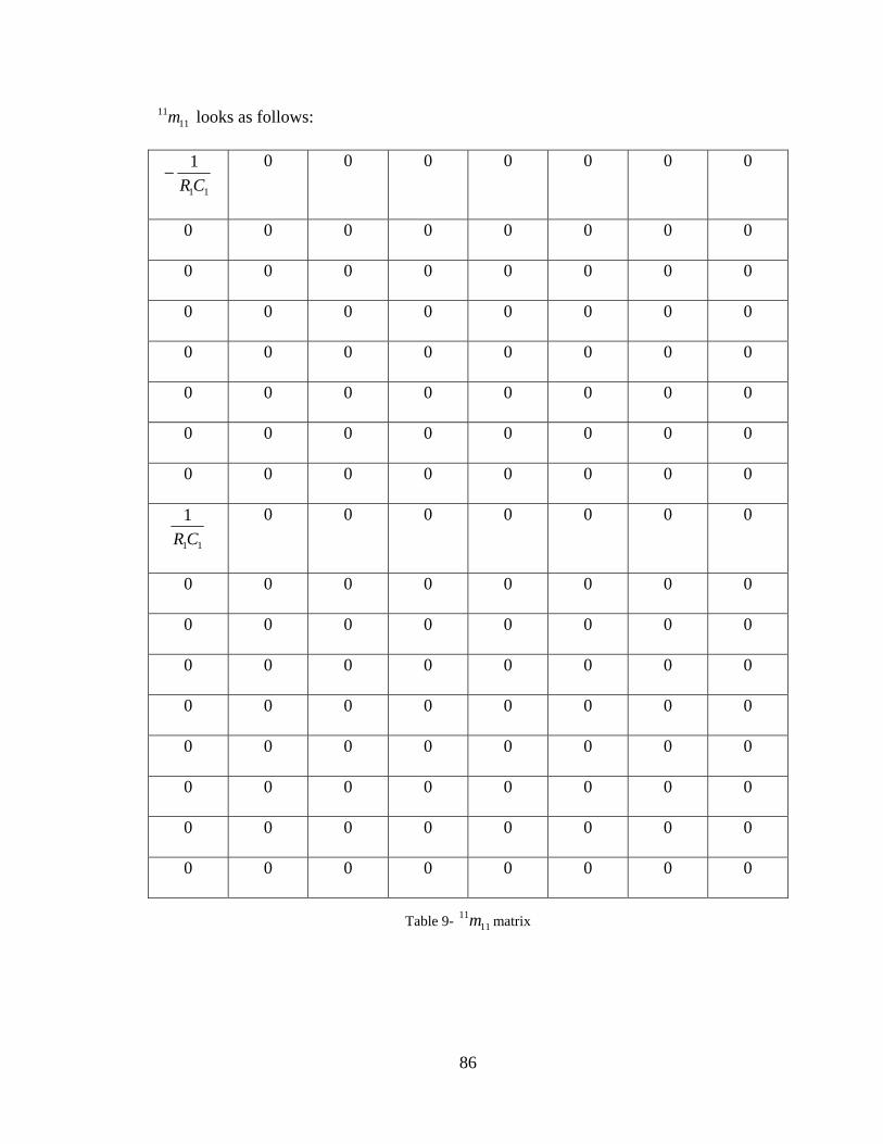
1111m looks as follows:

11

1CR

− 0 0 0 0 0 0 0

0 0 0 0 0 0 0 0

0 0 0 0 0 0 0 0

0 0 0 0 0 0 0 0

0 0 0 0 0 0 0 0

0 0 0 0 0 0 0 0

0 0 0 0 0 0 0 0

0 0 0 0 0 0 0 0

11CR1 0 0 0 0 0 0 0

0 0 0 0 0 0 0 0

0 0 0 0 0 0 0 0

0 0 0 0 0 0 0 0

0 0 0 0 0 0 0 0

0 0 0 0 0 0 0 0

0 0 0 0 0 0 0 0

0 0 0 0 0 0 0 0

0 0 0 0 0 0 0 0

Table 9- matrix 1111m

86

Due of entries in , it will be expressed as , where

and re res ctively and

to the large number 1211m [ ]bam =12

11

a b a 41 17pe 7× 5× matrice

Hence, has the following structure:

s.

−

−

a

11

1CR

'121

21

CRRRR +

− '12

1CR

0 0

'22

1CR

'232

32

CRRRR +

'23

1CR

'33

1CR

'343

43

CRRRR +

'34

1CR

'44

1CR

'454

54

CRRRR +

−

'55

1CR

0 0 0

0 0 0 0

0 0 0 0

0 0 0 0

0 0 0 0

0 0 0 0

0 0 0 0

0 0 0 0

0

0

0 0

0 0 0

0 0 0 0

0 0 0 0

87

0 0 0 0

0 0 0 0

[ ]bam =1211 Table 10- a matrix such that

And the fo owing structure:

0 0 0

b ll

0 0

0 0 0 0 0

0 0 0 0 0

0 0 0 0 0

0 0 0 0 0

0 0 0 0 0

0 0 0 0 0

'7C 8C

0 0 0 0 0

0 0 0 0 0

0 0 0 0 0

0 0 0 0 0

'45

1CR

0 0 0 0

'565

65

CRRRR +

− '56

1CR

0 0 0

'66

1CR

'676

76

CRRRR +

− '67

1CR

'7

'78

1CR

0

0 0

0

7

87

RRRR +

− 7

1R

88

0 0

8' '

88

1CR

−

12

0 0 0 0 0 0

−

1C

C

8

1CR

0

0 0 0 0 0

Table 11- matrix such that b [ ]bam =1211

Similarly if we now consider , it will have be a 8M ( ) ( )112 +×+ NN matrix, that is

with the following structure: 917×

1

1C

−

2

1C

−

3

1C

−

4

1C

5

1C

−

6

7

1C

−

8

1

'1

1C

'1

1C

− 0 0 0 0 0 0 0

0 0 0 0 0 0 0 0

0 0 0 0 0 0 0 0

0 0

0 0 0 0 0 0 0 0

0 0 0 0 0 0 0 0

0 0 0 0 0 − 0 0 0

0 0 0 0 0 0 0 0

0 0 0 0 0 0 0 − 0

89

0 '2

1C

'2

1C

−

'3

1C

'3

1C

−

' '

'5

1C

'5

1C

−

'6

1C

'6

1C

−

'7

1C

'7

1C

−

'8

1C

'8

1C

−

'9

1C

( )

218 mmM = here 21 and 21 are respectively , w 11m 12m × ices.

0 0 0 0 0 0

0 0 0 0 0 0 0

0 0 0

4 4C1

C 1

− 0 0 0 0

0 0 0 0 0 0 0

0 0 0 0 0 0 0

0 0 0 0 0 0 0

0 0 0 0 0 0 0

0 0 0 0 0 0 0 0

Table 12- matrix

’s size is ), i.e. it is a

128M

218M ( 121 +×+ NN 179× matrix with the following structure:

[ ]1221

1121 89× and matr

has the following structure:

99

1121m

1

1L

2

1L

0 0 0 0 0 0

0 0 0 0 0 0 0

0

90

0 0

0 0 0

0 0

0 0

0 0 0

0 0

0 0

3

1L

4

1L

5

1L

6

1L

7

1L

8

1L

0 0 0 0 0

0 0 0 0

0 0 0 0 0

0 0 0 0 0

0 0 0 0

0 0 0 0 0

0 0 0 0 0 0

Table 13- matrix

has the following structure:

1121m

1221m

1

1L

− 0 0 0 0 0 0 0 0

2

1L

2

1L

−

3 3

4

1L

4

1L

−

5

1L

5

1L

− 0 0 0 0

0 0 0 0 0 0 0

0 1L

1L

− 0 0 0 0 0 0

0 0 0 0 0 0 0

0 0 0

91

0 0 0 0

0 0 0 0 0 − 0 0

0 0 0 0 0 0 − 0

0 0 0 0 0 0 0 1

e 1 mat

th trix 22 1 +×

0

6

1L

6

1L

−

7

1L

7

1L

8

1L

8

1L

9

1L

9

0

0 0 0 0 0 0 0 0 0

0 0 0

L−

Tabl 4- rix

The last part of e

1221m

M8 ( ) ( )1

99×

ma is the 8M block which has a size of + NN ,

therefore it is a matrix full of zeros:

0 0 0 0 0 0 0 0

0 0 0 0 0 0 0 0 0

0 0 0 0 0 0 0 0 0

0 0 0 0 0 0 0 0 0

0 0 0 0 0 0 0 0 0

0 0 0 0 0 0 0 0

0 0 0 0 0 0 0 0 0

0 0 0 0 0 0 0 0 0

Table 15- matrix 228M

92

References:

[1] arthLin “Marx G erators http://h e.earthlink.net/~jimlux/hv/m x.htm E k, en ”, om ar

/m ner m

[2] Information Unlimited, “Marx Impulse Generators”, Accessed on 04/26/2006,

http://www.amazing1.com arx_ge ators.ht

[3] Andreas Kuthi, Ray Alde, Martin Gundersen and Andreas Neuber, “Marx Generator

Using PseudoSpark Switches” .

[4] S. Karni, “Intermediate Network Analysis”, Allyn and Bacon Inc. Boston, 1971.

[5] The MathWorks, “Optimization Toolbox for Use with MatLab”, version 3.

n Introduction”

a Class of Double-Rank Minimzation

Algorithms”, J. Inst. Maths. Applics. ol.6, pp -90, 19 .

[8] ariab m ”, Computer Journa ,

Vol. 13, pp 317-322, 1970.

[9] arb, D. “A Family of Variable Metr

Mathematics of Computing

[10] asi-Newton Methods for Function Minimization”,

Mathematics of Computing, Vol. 24, pp 647-656, 1970.

[11] Davidon, W.C. “Variable Metric Method for Minimization”, A.E.C. Research and

Development Report, ANL-5990, 1959.

[12] Fletcher, R. and M.J.D. Powell, “A Rapidly Convergent Descent Method for

Minimization”, Computer J ol. 6, pp 163-168, 1963.

[13] Georgia Institute of Technology System Realization Laboratory, “Quazi-Newton

Methods”, http://www.srl.gatech.edu/education/ME6103/Quasi-Newton.ppt.

[6] P. Dorato, C. Abdallah, V. Cerone, “Linear Quadratic Control a .

[7] Broyden, C.G. “The Convergence of

, V 76 70

Fletcher, R. “A New Approach to V le Metric Algorith s l

Goldf ic Updates Derived by Variational Means”,

, Vol. 24, pp 23-26, 1970.

Shanno, D.F., “Conditioning of Qu

ournal, V

93