state of wyoming - us department of energy filestate of wyoming technical support document i ... 1...
TRANSCRIPT

STATE OF WYOMING
Technical Support Document I
For Recommended 8-Hour Ozone Designation
For the Upper Green River Basin, WY
March 26, 2009
The Wyoming Department of Environmental Quality
Air Quality Division
Herschler Building, 122 West 25th
Street
Cheyenne, Wyoming 82002

i
Table of Contents
Page
Executive Summary ..................................................................................................................... vi
Introduction ....................................................................................................................................1
Background and Regulatory History ...................................................................................1
Basis for Technical Support .................................................................................................1
Recommended Nonattainment Area Boundary ...................................................................1
Key Issues ............................................................................................................................3
Section 1. Air Quality Data ..........................................................................................................5
Synopsis ...............................................................................................................................5
Analysis................................................................................................................................5
Section 2. Emissions Data ...........................................................................................................12
Synopsis .............................................................................................................................12
Analysis..............................................................................................................................12
Biogenics................................................................................................................12
Oil and Gas Production and Development.............................................................13
Section 3. Population Density and Degree of Urbanization ....................................................17
Synopsis .............................................................................................................................17
Analysis..............................................................................................................................17
Section 4. Traffic and Commuting Patterns .............................................................................20
Synopsis .............................................................................................................................20
Analysis..............................................................................................................................20
Section 5. Growth Rates and Patterns ......................................................................................23
Synopsis .............................................................................................................................23
Analysis..............................................................................................................................23
Section 6. Geography/Topography ............................................................................................27
Synopsis .............................................................................................................................27
Analysis..............................................................................................................................27
Section 7. Meteorology................................................................................................................31
Synopsis .............................................................................................................................31
Analysis..............................................................................................................................31
General ...................................................................................................................31
Winter Ozone field Studies ....................................................................................32
Comparison of 2007 and 2008 Field Study Observations .....................................34
Snow Cover and Sunlight ..........................................................................34
Low Wind Speeds ......................................................................................34
Ozone Carryover ........................................................................................35

ii
Atmospheric Mixing ..................................................................................36
Feb. 19-23, 2008 Case Study Illustrating the Specific Weather
Conditions Which Produce Elevated Ozone in the Upper Green
River Basin.................................................................................................36
Synopsis of 19-23 February 2008 Ozone Episode .................................................37
Description of Surface Wind Data .........................................................................39
Description of Conditions Aloft.............................................................................44
Tools to Evaluate Precursor Emissions and Transport: HYSPLIT vs.
AQplot Back Trajectory Analysis ..........................................................................47
AQplot Back Trajectory Analysis ..........................................................................52
CalDESK Trajectory Analysis ...............................................................................53
Specific Examples of Trajectory Analyses Using CalDESK ....................55
Summary of Trajectory Analyses ..........................................................................86
Section 8. Jurisdictional Boundaries .........................................................................................87
Synopsis .............................................................................................................................87
Analysis..............................................................................................................................87
Section 9. Level of Control of Emission Sources ......................................................................88
Synopsis .............................................................................................................................88
Analysis..............................................................................................................................88
New Source Review Program ................................................................................88
Best Available Control Technology...........................................................88
Control of Oil and Gas Production Sources ...............................................89
Statewide and Industry-wide Control of Volatile Organic Compounds (VOC) ....90
Statewide and Industry-wide Nitrogen Oxides (NOx)...........................................92
Contingency Plans .................................................................................................93
Conclusions ...................................................................................................................................94
List of Tables
Table S.1-1: Design Values for Monitors In or Near the Upper Green River Basin ......................7
Table S.1-2: 4th
Maximum 8-Hour Ozone Values for Monitoring in Surrounding Counties .........8
Table S.2-1: 1st Quarter, 2007 Estimated Emissions Summary (tons) .........................................14
Table S.3-1: Population Density ...................................................................................................17
Table S.3-2: Population Estimates and Projections ......................................................................18
Table S.3-3: Population Growth ...................................................................................................19
Table S.3-4: Distance to Boulder Monitor ....................................................................................19
Table S.4-1: WYDOT - 2007 Traffic Surveys..............................................................................21
Table S.4-2: Wyoming DOE Commuter Surveys 2000 Through 2005 ........................................21
Table S.4-3: Number of Commuters in Sublette and Surrounding Counties ...............................22
Table S.5-1: Completion Report Sublette County ........................................................................23
Table S.5-2: Total Well Completions/Oil, Gas, and CBM ...........................................................24
Table S.5-3: Sublette County Production Levels ..........................................................................25
Table S.5-4: Four County Production ...........................................................................................26

iii
Table S.7-1: Summary of daily maximum 8-hour averaged ozone concentrations
monitored at the Jonah, Boulder, and Daniel monitors during February 18-23 ......36
Table S.7-2: Summary of the low-level inversion measurements, and related data on
inversion strength in the surface-based stable layer ................................................45
List of Figures
Figure S.1-1: Map Showing Monitoring Stations In and Near the Upper Green River .................6
Figure S.1-2: Monthly 8-Hour Maximum Ozone Within the UGRB .............................................9
Figure S.1-3: Winter 2009 Ozone Monitoring in the Upper Green River Basin ..........................11
Figure S.2-1: Estimated Upper Green River Basin Emissions 1st Quarter, 2007 .........................15
Figure S.2-2: Designation Area Boundary....................................................................................16
Figure S.5-1: Well Completions Per County ................................................................................24
Figure S.5-2: Sublette County Gas Production .............................................................................25
Figure S.6-1: Nonattainment area shown (blue outline) against an aerial view of the
topography in the Upper Green River Basin and adjacent areas ............................28
Figure S.6-2: Transects across the Upper Green River Basin (running north-south and
east-west) showing cross sections of the terrain; terrain elevations and distance
units shown in the transects are in meters ...............................................................29
Figure S.7-1: Location of surface and upper air monitoring sites employed in 2008
field study................................................................................................................33
Figure S.7-2: Wind speed and ozone concentrations plotted for the Boulder monitor in
February and March 2008 ......................................................................................35
Figure S.7-3: Constant pressure map for 700 mb, morning 02/19/08 (1200 UTC)
[(5 am LST)] ...........................................................................................................37
Figure S.7-4: Constant pressure map for 700 mb, 02/22/08 (0000 UTC) [02/21/08 (5 pm
LST)] ......................................................................................................................38
Figure S.7-5: Composite wind rose map for February 18-22, 2008 at monitoring sites
located throughout Southwest Wyoming ...............................................................40
Figure S.7-6: Time-series showing February 20, 2008 hourly wind vectors for monitors
used in 2008 field study monitoring network ........................................................41
Figure S.7-7: Time-series showing February 21, 2008 hourly wind vectors for monitors
used in 2008 field study monitoring network ........................................................42
Figure S.7-8: Wind roses based on 15:00 (MST) data from the Boulder site for days
with maximum 8-hour average ozone a) greater than 74 ppb (left) and b) less
than 76 ppb (right) .................................................................................................43
Figure S.7-9: SODAR-reported mixing height versus peak daily 8-hour ozone
concentrations at Boulder. Measurements limited to below approximately
250 meters above ground level (AGL) ...................................................................46
Figure S.7-10: February 21, 2008 balloon-borne soundings; Sounding at 11:00 (MST)
(left); Sounding at 16:00 (MST) (right) ................................................................47
Figure S.7-11: A comparison of the local terrain features at 1 km and 40 km
resolution, respectively, and the resulting “smoothed” terrain as shown
in the 40 km 3-D topographic plot .......................................................................48
Figure S.7-12: A comparison of the local terrain features at 1 km and 40 km resolution,
respectively, as depicted in the 2-D contour plots ................................................49

iv
Figure S.7-13: Comparison of HYSPLIT (red) and AQplot (pink) 12-hour back
trajectories from the Boulder monitoring site on February 20, 2008 ...................51
Figure S.7-14: Comparison of HYSPLIT (red) and AQplot (green) 12-hour back
trajectories from the Jonah monitoring site on February 20, 2008 ......................51
Figure S.7-15: 12-hour back trajectories from field study monitoring sites on
February 20, 2008 .................................................................................................52
Figure S.7-16: Terrain features represented in CALMET modeling domain (464 km x
400 km) ................................................................................................................54
Figure S.7-17: CALMET wind field at 4:00 am (MST) on February 20, 2008. The
2008 field study meteorological monitoring sites are shown for reference ..........54
Figure S.7-18: 24-hour forward trajectory analysis at LaBarge, Wyoming on
February 18, 2008 .................................................................................................56
Figure S.7-19: 24-hour forward trajectory analysis in the Moxa Arch area on
February 18, 2008 .................................................................................................57
Figure S.7-20: 24-hour forward trajectory analysis at Naughton power plant on
February 18, 2008 .................................................................................................58
Figure S.7-21: 24-hour forward trajectory analysis at OCI Trona plant on
February 18, 2008 .................................................................................................59
Figure S.7-22: 24-hour forward trajectory analysis at Bridger power plant on
February 18, 2008 .................................................................................................60
Figure S.7-23: 24-hour forward trajectory analysis at LaBarge, Wyoming on
February 19, 2008. ................................................................................................61
Figure S.7-24: 24-hour forward trajectory analysis in the Moxa Arch area on
February 19, 2008 .................................................................................................62
Figure S.7-25: 24-hour forward trajectory analysis at Naughton power plant on
February 19, 2008 .................................................................................................63
Figure S.7-26: 24-hour forward trajectory analysis at OCI Trona plant on
February 19, 2008 .................................................................................................64
Figure S.7-27: 24-hour forward trajectory analysis at Bridger power plant on
February 19, 2008 .................................................................................................65
Figure S.7-28: 24-hour forward trajectory analysis at LaBarge, Wyoming on
February 20, 2008 .................................................................................................66
Figure S.7-29: 24-hour forward trajectory analysis in the Moxa Arch area on
February 20, 2008 .................................................................................................67
Figure S.7-30: 24-hour forward trajectory analysis at Naughton power plant on
February 20, 2008 .................................................................................................68
Figure S.7-31: 24-hour forward trajectory analysis at OCI Trona plant on
February 20, 2008 .................................................................................................69
Figure S.7-32: 24-hour forward trajectory analysis at Bridger power plant on
February 20, 2008 .................................................................................................70
Figure S.7-33: 24-hour forward trajectory analysis at LaBarge, Wyoming on
February 21, 2008 .................................................................................................71
Figure S.7-34: 24-hour forward trajectory analysis in the Moxa Arch area on
February 21, 2008 .................................................................................................72

v
Figure S.7-35: 24-hour forward trajectory analysis at Naughton power plant on
February 21, 2008 .................................................................................................73
Figure S.7-36: 24-hour forward trajectory analysis at OCI Trona plant on
February 21, 2008 .................................................................................................74
Figure S.7-37: 24-hour forward trajectory analysis at Bridger power plant on
February 21, 2008 .................................................................................................75
Figure S.7-38: 24-hour forward trajectory analysis at LaBarge, Wyoming on
February 22, 2008 .................................................................................................76
Figure S.7-39: 24-hour forward trajectory analysis in the Moxa Arch area on
February 22, 2008 .................................................................................................77
Figure S.7-40: 24-hour forward trajectory analysis at Naughton power plant on
February 22, 2008 .................................................................................................78
Figure S.7-41: 12-hour back trajectory analysis at Boulder monitor on February 22, 2008 ........79
Figure S.7-42: 24-hour forward trajectory analysis at OCI Trona plant on
February 22, 2008 .................................................................................................80
Figure S.7-43: 24-hour forward trajectory analysis at Bridger power plant on
February 22, 2008 .................................................................................................81
Figure S.7-44: 24-hour forward trajectory analysis at LaBarge, Wyoming on
February 23, 2008 .................................................................................................82
Figure S.7-45: 24-hour forward trajectory analysis in the Moxa Arch area on
February 23, 2008 .................................................................................................83
Figure S.7-46: 24-hour forward trajectory analysis at Naughton power plant on
February 23, 2008 .................................................................................................84
Figure S.7-47: 24-hour forward trajectory analysis at OCI Trona plant on
February 23, 2008 .................................................................................................85
Figure S.7-48: 24-hour forward trajectory analysis at Bridger power plant on
February 23, 2008 .................................................................................................86
List of Appendices
Appendix S.1. Final Report 2008 Upper Green River Winter Ozone Study
Appendix S.3. Population Density by Census Tract
Appendix S.4.A. 2007 Vehicle Miles on State Highways By County
Appendix S.4.B. Commuting Patterns in Sublette County
Appendix. Glossary

vi
EXECUTIVE SUMMARY
In March 2008 the US EPA promulgated a new National Ambient Air Quality Standard
(NAAQS) for ozone. The new standard was lowered from 0.08 ppm to 0.075 ppm based on the
fourth highest 8-hour average value per year at a site, averaged over three years. Based on
monitoring results from 2006 through 2008, the entire state of Wyoming is in compliance with
this standard except for at a single monitor, the Boulder monitor, in Sublette County.
The Wyoming Department of Environmental Quality, Air Quality Division (AQD) evaluated
whether a nonattainment area should be designated due to the monitored results at the Boulder
monitor. Using EPA’s guidance in the Robert J. Meyers December 4, 2008 memo, the AQD
performed a nine-factor analysis, which is the basis of this document. This analysis supports
AQD’s recommendation that the Upper Green River Basin (UGRB), as defined in the
introduction to this document, be designated as nonattainment for the 2008 ozone NAAQS.
The AQD bases this recommendation on a careful review of the circumstances surrounding the
incidence of elevated ozone events. Elevated ozone in the UGRB is associated with distinct
meteorological conditions. These conditions have occurred in February and March in some (but
not all) of the years since monitoring stations began operation in the UGRB in 2005. Our
determination of an appropriate nonattainment area boundary is focused on an evaluation of
EPA’s nine factors, applied to the first quarter of the year. It is important to evaluate conditions
during the first quarter of the year in order to focus on the very specific set of circumstances that
lead to high ozone.
The most compelling reasons for the boundary recommendation are based on the meteorological
conditions in place during and just prior to elevated ozone events. Elevated ozone episodes
occurred in 2005, 2006 and 2008; they were associated with very light low-level winds,
sunshine, and snow cover, in conjunction with a strong low-level surface-based temperature or
“capping” inversion. The longest such event (February 19-23, 2008), which also resulted in the
highest measured ozone of 122 ppb as an 8-hour average at the Boulder station, has been
reviewed in detail and summarized in Section 7 of this document. Section 7 demonstrates that
sources outside the recommended nonattainment area would not have a significant impact on the
Boulder monitor due to the presence of an inversion and very low wind speeds, which
significantly limit precursor and ozone transport from sources located outside of the UGRB.
The AQD carefully examined sources of ozone and ozone precursors within Sublette and
surrounding counties. When evaluating sources, AQD considered these five of EPA’s factors:
population density, traffic and commuting patterns, growth rates and patterns, emission data, and
level of control of air emissions. Sublette County is a rural county with a population density of
two people per square mile; the most densely populated nearby county (Uinta) is also largely
rural with a population density of ten people per square mile. As would be expected, the number
of commuters into or out of the UGRB is small and does not represent a significant source of
precursor emissions. While there is an interstate highway 80 miles south of the Boulder monitor,
the attached analysis demonstrates that I-80 traffic is not considered to be a significant
contributor of emissions that impact the Boulder monitor during ozone events.

vii
Although population and population growth was not a significant factor, growth in the oil and
gas (O&G) industry in Sublette County was considered pertinent. The volume of natural gas
produced doubled between 2000 and 2008 in the county; the number of wells completed doubled
between 2004 and 2008. Approximately 1,500 well completions were recorded in Sublette
County in the last four years. Growth in the oil and gas industry in nearby areas is much slower.
AQD prepared an estimated inventory of emissions for the recommended nonattainment area and
the surrounding counties. The inventory showed that approximately 94% of VOC emissions in
the UGRB and 60% of NOx emissions are attributable to oil and gas production and
development. Of the eleven major sources in the UGRB, all are O&G related. To the north, east
and west there are few major sources in counties adjacent to the UGRB. In addition to the major
sources, there are numerous minor sources in the UGRB including several concentrated areas of
O&G development. Just to the south of the UGRB, there are a few major sources, several minor
sources and again, a concentrated area of O&G wells. AQD then used other factors,
meteorology, topography, and level of control of emissions, to determine which of the sources to
the south of Sublette County should be included in the proposed nonattainment boundary.
The level of control of emissions in the Jonah and Pinedale Anticline Development is very
stringent and new oil and gas production units in Sublette County and surrounding counties
require permits including Best Available Control Technology (BACT). An interim policy for
Sublette County which took effect in 2008 results in a net decrease in emissions of ozone
precursors with every permit that is issued. Since stricter controls for O&G are already in place
in Sublette County, if O&G sources outside of Sublette County might contribute ozone or ozone
precursors to the Boulder monitor, including these O&G sources in the proposed nonattainment
area would provide motivation to control these sources.
In evaluating topography, the east, north and west county boundaries are natural boundaries of
high mountains. These geographical and jurisdictional boundaries also coincide with population
boundaries and emission source boundaries. To the south, the topographical boundaries are less
dramatic, but there are rivers, valleys, and buttes that form geographic boundaries near the
southern border of Sublette County. Therefore, the AQD considered the county boundary to the
north, east and west to be a reasonable boundary based on geography, jurisdictions, emission
sources, population and growth.
However, meteorology provided the strongest basis for setting the southern boundary of the
proposed nonattainment area. Elevated ozone in the UGRB is associated with distinct
meteorological conditions. These conditions have occurred in February and March in some (but
not all) of the years since monitoring stations began operation in the UGRB in 2005.
Meteorological conditions in place during and just prior to elevated ozone events provide the
most specific data for setting the south boundary. Elevated ozone episodes are associated with
very light low-level winds, cold temperatures, sunshine, and snow cover, in conjunction with
strong low-level surface-based temperature inversions. Sources outside the recommended
nonattainment area would not have a significant impact on the Boulder monitor due to the
presence of an inversion and the very low wind speeds, which influence the transport of

viii
emissions. Detailed meteorological data collected during intensive field studies shows that
emissions from sources south of the recommended nonattainment area are generally carried
toward the east and not into the UGRB during or just prior to an ozone episode. Speciated VOC
data collected in the UGRB during elevated ozone episodes also has a dominant oil and gas
signature, indicating the VOC concentrations are largely due to O&G development activities.
Meteorology and topography indicate that sources outside a southern boundary defined by the
Little Sand Creek and Pacific Creek to the east and the Green River and Fontenelle Creek to the
west do not contribute to ozone and ozone precursors which could affect the Boulder monitor.
The analysis conclusively shows that elevated ozone at the Boulder monitor is primarily due to
local emissions from oil and gas (O&G) development activities: drilling, production, storage,
transport, and treating. The ozone exceedances only occur when winds are low indicating that
there is no transport of ozone or precursors from distances outside the proposed nonattainment
area. The ozone exceedances only occur in the winter when the following conditions are present:
strong temperature inversions, low winds, cold temperatures, clear skies and snow cover. If
transport from outside the proposed nonattainment area was contributing to the exceedances,
then elevated ozone would be expected at other times of the year. Mountain ranges with peaks
over 10,000 feet border the area to the west, north and east influence the local wind patterns.
Emission sources in nearby counties are not upwind of the Boulder monitor during episodes
which exceed the 8-hour ozone standard in Sublette County.
The proposed nonattainment area boundary includes the violating monitor and the sources which
are most likely to contribute ozone and ozone precursors to the monitored area. Using this as a
boundary will allow the State to focus its resources on the emission sources that contribute to the
ozone issue and will allow the State to control the ozone problem in a timely manner.

1
INTRODUCTION
BACKGROUND AND REGULATORY HISTORY
The U.S. Environmental Protection Agency (EPA) is charged with developing air quality
standards for the protection of human health and welfare. EPA is also required to periodically
evaluate those standards and revise them if scientific analyses indicate different standards would
be more protective of public health and welfare. In March of 2008, EPA promulgated a new
National Ambient Air Quality Standard (NAAQS) for ozone. This new standard lowered the 8-
hour level of ozone from 0.08 parts per million (ppm) to 0.075 ppm, based on the fourth
maximum 8-hour value at a site averaged over three years. Each state must recommend ozone
designations no later than March 12, 2009 and final designations must be complete by March 12,
2010.
BASIS FOR TECHNICAL SUPPORT
This technical support document considers nine criteria, or “factors” to make a recommendation
for the appropriate location and boundary of a nonattainment area. Those factors are derived
from EPA’s memorandum issued December 4, 2008, “Area Designations for the 2008 Revised
Ozone National Ambient Air Quality Standards.” States must submit an analysis of these nine
factors, along with a proposed nonattainment boundary, for any areas that are not meeting the
federal standard. The nine factors that must be addressed are:
Air quality data
Emissions data (location of sources and contribution to ozone concentrations)
Population density and degree of urbanization (including commercial development)
Traffic and commuting patterns
Growth rates and patterns
Meteorology (weather/transport patterns)
Geography/topography (mountain ranges or other air basin boundaries)
Jurisdictional boundaries (e.g., counties, air districts, existing nonattainment areas,
Reservations, metropolitan planning organizations (MPOs))
Level of control of air emissions
RECOMMENDED NONATTAINMENT AREA BOUNDARY
The State of Wyoming recommends that the UGRB, with boundaries described as follows, be
designated as a nonattainment area for the 2008 8-hour ozone standard:
Sublette County: (all)
Lincoln County: (part) The area of the county north and east of the boundary defined by a
line starting at the point defined by the intersection of the southwest corner Section 30 Range

2
(R) 115 West Township (T) 27N and the northwest corner of Section 31 R 115 West T 27N
of Sublette County at Sublette County’s border with Lincoln County. From this point the
boundary moves to the west 500 feet to Aspen Creek. The boundary follows the centerline
of Aspen Creek downstream to the confluence of Aspen Creek and Fontenelle Creek (in R
116 W T26N, Section 1). From this point the boundary moves generally to the south along
the centerline of Fontenelle Creek to the confluence of Fontenelle Creek and Roney Creek (in
R115W T24N Section 6). From the confluence, the boundary moves generally to the east
along the centerline of Fontenelle Creek and into the Fontenelle Reservoir (in R112W T24N
Section 6). The boundary moves east southeast along the centerline of the Fontenelle
Reservoir and then toward the south along the centerline of the Green River to where the
Green River in R111W T24 N Section 31 crosses into Sweetwater County.
Sweetwater County: (part) The area of the county west and north of the boundary which
begins at the midpoint of the Green River, where the Green River enters Sweetwater County
from Lincoln County in R111W T24N Section 31. From this point, the boundary follows the
center of the channel of the Green River generally to the south and east to the confluence of
the Green River and the Big Sandy River (in R109W R22 N Section 28). From this point,
the boundary moves generally north and east along the centerline of the Big Sandy River to
the confluence of the Big Sandy River with Little Sandy Creek (in R106W T25N Section
33). The boundary continues generally toward the northeast along the centerline of Little
Sandy Creek to the confluence of Little Sandy Creek and Pacific Creek (in R106W T25N
Section 24). From this point, the boundary moves generally to the east and north along the
centerline of Pacific Creek to the confluence of Pacific Creek and Whitehorse Creek (in
R103W T26N Section 10). From this point the boundary follows the centerline of
Whitehorse Creek generally to the northeast until it reaches the eastern boundary of Section 1
R103W T 26North. From the point where Whitehorse Creek crosses the eastern section line
of Section 1 R103W T 26North, the boundary moves straight north along the section line to
the southeast corner of Section 36 R103W T27N in Sublette County where the boundary
ends.
A picture of this area follows.
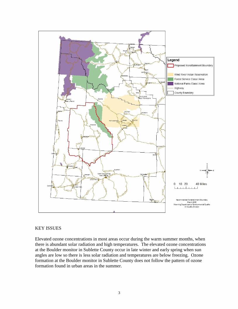
3
KEY ISSUES
Elevated ozone concentrations in most areas occur during the warm summer months, when
there is abundant solar radiation and high temperatures. The elevated ozone concentrations
at the Boulder monitor in Sublette County occur in late winter and early spring when sun
angles are low so there is less solar radiation and temperatures are below freezing. Ozone
formation at the Boulder monitor in Sublette County does not follow the pattern of ozone
formation found in urban areas in the summer.

4
Moderately elevated ozone was first detected in Sublette County in February of 2005 and
2006. The Wyoming Air Quality Division (AQD) conducted intensive meteorological and
ambient data collection and analyses in 2007 and 2008 in order to understand this
phenomenon. AQD is continuing this effort in 2009. Although analysis of all the data is not
complete, AQD has already determined that:
Local meteorological conditions are the single most important factor contributing to
the formation of ozone and the definition of the nonattainment boundary.
Meteorological models that utilize only regional data will not correctly attribute
ozone and ozone precursors to the sources which affect the UGRB.
Trajectory analyses using detailed observation-based wind field data show that local
scale transport of ozone and ozone precursors is dominant during periods of elevated
ozone.
Trajectory analyses using the wind field data show that regional transport of ozone
and ozone precursors appears to be insignificant during periods of elevated ozone.

5
SECTION 1
AIR QUALITY DATA SYNOPSIS
Ozone at levels exceeding the standard has been monitored at one of three stations in the UGRB
– specifically, the Boulder monitor.
Measured ozone levels have not exceeded the standard in the counties adjacent to the UGRB.
Elevated ozone within the UGRB typically only occurs in January, February, or March.
VOCs detected in ambient air in the UGRB have a strong oil and gas signature.
ANALYSIS
The Wyoming Air Quality Division (AQD) operated three monitoring stations in the proposed
nonattainment area in 2005-2008. Monitor locations are shown on the map in Figure S.1-1. This
map also shows the location of monitors in adjacent counties.
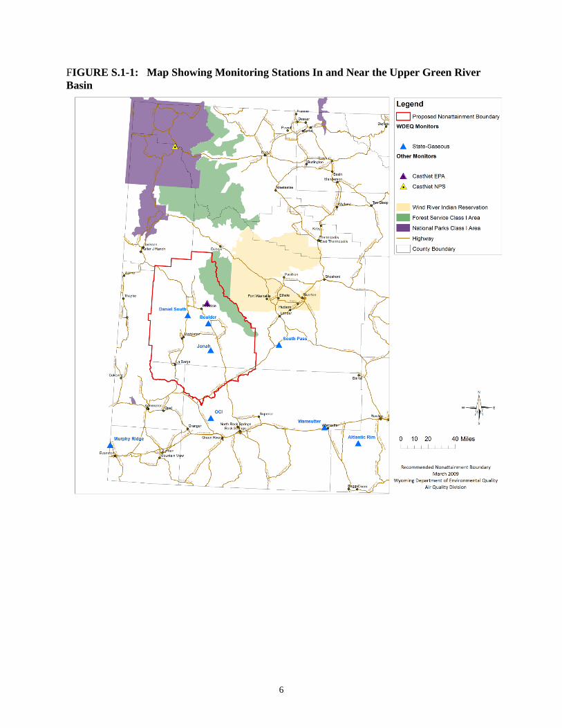
6
FIGURE S.1-1: Map Showing Monitoring Stations In and Near the Upper Green River
Basin

7
Table S.1-1 shows the ozone design values for the 8-hour standard for the Reference or
Equivalent Method monitoring stations shown in Figure S.1-1. All data are collected by
Reference or Equivalent Method monitors and meet EPA’s criteria for quality and completeness
unless otherwise noted. Please note, Pinedale CASTNet data are not included in the design
values because this station was not operated in accordance with Part 58 QA requirements until
2007. The design value is the three-year average of the annual fourth highest daily maximum 8-
hour ozone concentration (a calculated value less than or equal to 0.075 ppm indicates attainment
of the standard; a calculated value of greater than 0.075 ppm is a violation of the standard).
Table S.1-2 shows monitored data from other Federal Reference Method (FRM) or Federal
Equivalent Method (FEM) ozone monitors in the counties surrounding the UGRB. These
monitors have been running for less than 3 years and therefore do not have a design value
calculated.
Table S.1-1: Design Values for Monitors In or Near the Upper Green River Basin
Site Name AQS ID
Year 3-Year
Average
2005-2007
(ppm)
3-Year
Average
2006-20081
(ppm)
2005
(ppm)
2006
(ppm)
2007
(ppm)
2008
Q1 – Q3
(ppm)
Daniel South 56-035-0100 0.0672 0.075 0.067 0.074
N/A
0.072
1
Boulder 56-035-0099 0.0803 0.073 0.067 0.101
0.073
3 0.080
1
Jonah 56-035-0098 0.076 0.070 0.069 0.082
0.072 0.0741
Yellowstone
(NPS) 56-039-1011 0.060 0.069 0.064 0.065 0.064 0.066
1 Data collected and validated through 3
rd quarter 2008
2 Incomplete year; began operation in July 2005
3 Incomplete year; began operation in February 2005

8
Table S.1-2: 4th
Maximum 8-Hour Ozone Values for Monitoring in
Surrounding Counties
Site Name AQS ID
Year
2005
(ppm)
2006
(ppm)
2007
(ppm)
2008
Q1 – Q3
(ppm)
Murphy Ridge 56-041-0101 --- --- 0.070 0.0611
South Pass 56-013-0099 --- --- 0.0712
0.0651
OCI3
56-037-0898 --- 0.0713
0.066 0.0721
Wamsutter 56-005-0123 --- 0.0674
0.064 0.0641
Atlantic Rim 56-007-0099 --- --- 0.0475
0.0641
1 Data collected and validated through 3
rd quarter 2008
2 Incomplete year; began operation in March 2007
3 Site operated by industry. Incomplete year; began operation in May 2006
4 Incomplete year; began operation in March 2006
5 Incomplete year; began operation in October 2007
Using only data from 2005 through 2007, the monitors for which a design value can be
calculated indicate compliance with the ozone NAAQS. Year-to-date data from 2008, however,
bring the 2006 - 2008 design value for the Boulder monitor to 0.080 ppm (compared to the
standard of 0.075).
While monitors in counties adjacent to the UGRB have not been in operation for a full three-year
period (with the exception of the Yellowstone NPS monitor), none of them have 4th
-high
maximum 8-hour ozone values above 0.075 ppm for any year. This would indicate that, based
on ambient monitoring data, ozone levels have not been measured that exceed the standard
outside of the UGRB (within Wyoming).
When the data from the Boulder monitoring station, the only monitor showing ozone levels in
excess of the standard, is reviewed closely, it shows that elevated ozone typically occurs in the
winter. This trend is also evident at the two stations nearby (South Daniel and Jonah). Figure
S.1-2 shows the daily 8-hour maximum for these stations on a monthly basis over the last four
years. This is an unprecedented phenomenon, as ozone was thought to be a summertime
problem. The Wyoming DEQ, with the help of industry, has dedicated significant resources to
better understand this situation. The studies indicate that elevated ozone occurs in the UGRB
under very specific meteorological conditions, described in greater detail in Section 7 of this
document. Briefly, these conditions are the presence of a strong temperature inversion in
conjunction with low wind speeds, snow cover and clear skies. These conditions have occurred
in January, February, and March.

9
Figure S.1-2: Monthly 8-Hour Maximum Ozone Within the UGRB
AQD performed Winter Ozone Studies in 2007, 2008 and 2009 in the UGRB. The purpose of
these studies is to investigate and monitor the mechanisms of ozone formation during the winter
months. These data will in turn be used to develop a conceptual model of ozone formation in the
UGRB. As the study has progressed, the scope of the study has been refined as AQD has learned
about the unique issue of winter ozone formation. In general terms, the scope of the winter
ozone studies include:
1. Placing additional FEM and non-FEM (2B ozone analyzers) monitors throughout the
UGRB to characterize spatial and temporal distribution of ground-level ozone.
2. Placing additional three-meter meteorological towers (mesonet) throughout the UGRB to
characterize local micro-scale meteorology.
3. Placing additional precursor monitoring (e.g., VOC, NOx and CO) in a few sites around
the UGRB to characterize precursor concentrations.
4. Flying a plane equipped with continuous ozone and PM2.5 around the UGRB to
characterize spatial distribution of ozone (above, in, and below the boundary layer).
5. Launching ozone and rawinsondes to characterize vertical meteorology and ozone
distribution.
25
35
45
55
65
75
85
95
105
115
125
Jan-05 Jul-05 Jan-06 Jul-06 Jan-07 Jul-07 Jan-08 Jul-08 Jan-09
Ozo
ne
(p
pb
)
Boulder maximum
Jonah maximum
Daniel maximum

10
6. Operating ground based upper-air meteorological instruments (e.g., Mini-SODAR,
RASS, Wind Profiler) to characterize mixing levels and inversion heights.
In 2007, meteorological conditions did not set up as they had in 2005 and 2006 and elevated
ozone did not form in February and March. However, AQD collected data that helped to draw
some conclusions about winter ozone formation. The speciated VOC samples collected had a
strong oil and gas signature. AQD was able to investigate which detected VOC species were
having a greater effect on ozone formation. UV radiation measurements showed that when fresh
snow is available, greater than 80% of the ultra-violet light can be reflected.
During the 2008 winter study, several multi-day episodes of elevated ozone were studied. Six
additional ozone monitoring locations were added and the plane was flown to provide more
information on the spatial and temporal variability around the UGRB. AQD continued to collect
speciated VOC samples which confirmed the strong oil and gas signature. These data also
allowed us to identify species of interest with respect to elevated ozone formation. AQD also
used a mini-SODAR and rawinsondes to characterize the mixing heights and inversion strength
on elevated ozone days. It was found that on days with elevated ozone, mixing heights could be
as shallow as 50-200 meters above ground level.
For the 2009 winter study, AQD has placed eleven FEM and non-FEM continuous ozone
monitors around the UGRB. Additionally, AQD has placed five FEM ozone monitors in
communities around the UGRB as part of an Air Toxics study. These monitors compliment the
three long-term FEM ozone monitors currently operating. AQD has also added precursor
monitoring at the Boulder, Jonah and SODAR stations. Figure S.1-3 shows the current
configuration of ozone monitoring in the UGRB.
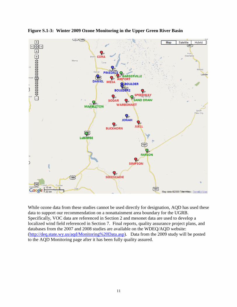
11
Figure S.1-3: Winter 2009 Ozone Monitoring in the Upper Green River Basin
While ozone data from these studies cannot be used directly for designation, AQD has used these
data to support our recommendation on a nonattainment area boundary for the UGRB.
Specifically, VOC data are referenced in Section 2 and mesonet data are used to develop a
localized wind field referenced in Section 7. Final reports, quality assurance project plans, and
databases from the 2007 and 2008 studies are available on the WDEQ/AQD website:
(http://deq.state.wy.us/aqd/Monitoring%20Data.asp). Data from the 2009 study will be posted
to the AQD Monitoring page after it has been fully quality assured.

12
SECTION 2
EMISSIONS DATA
SYNOPSIS
The primary sources of ozone-forming precursors in the recommended nonattainment area are
associated with the oil and gas development and production industry in the UGRB.
ANALYSIS
Ground-level ozone is primarily formed from reactions of volatile organic compounds (VOCs)
and oxides of nitrogen (NOx) in the presence of sunlight. VOCs and NOx are considered “ozone
precursors.” As part of the nine-factor analysis, the Air Quality Division compiled emission
estimates for VOCs and NOx for ten source categories in the proposed nonattainment area as
well as counties or portions of counties surrounding the area. This information is summarized in
Table S.2-1 and represents preliminary estimated first quarter 2007 emission inventory data for
all potential sources. Emissions information for 2007 is used because it is the most recently
available data for all source sectors. Only the first quarter is shown because elevated ozone in
the UGRB occurs during limited episodes in the first three months of the calendar year. In
general, quarterly emissions for the second through fourth quarters of the year are the same as for
the first quarter, with the exception that biogenic VOC emissions are expected to be greater in
the spring and summer months.
When comparing the raw precursor emission totals in Table S.2-1, AQD is aware that the total
for the area defined as “Sweetwater Outside of Upper Green River Basin” is the largest for both
VOCs and NOx. However, after carefully reviewing the other eight factors to determine an
appropriate boundary, AQD has concluded that there are no violations occurring in Sweetwater
County, nor are the emissions sources in most of Sweetwater County contributing meaningfully
to the observed violations in Sublette County. AQD will demonstrate in this document that the
emissions identified in the UGRB, along with other key factors such as site-specific air quality
data (Section 1), unique meteorological and geographical conditions (Sections 6 and 7), as well
as extraordinary industrial growth rates (Section 5), will explain the exceedances of the ozone
standard at the Boulder monitor in Sublette County.
AQD has taken the next step to focus in on the particular emission sources believed to be
contributing to high ozone levels. Figure S.2-1 shows emission inventory data for the UGRB.
These emission estimates indicate that the most significant sources of ozone precursors in the
UGRB are biogenics and the oil and gas industry.
Biogenics
During the first quarter of the year, biogenic emissions are lower than emissions from the other
months of the year. The 2007 and 2008 Upper Green Winter Ozone Study (described in Section
1) analyzed canister samples for four biogenic species: isoprene, a-pinene, b-pinene, and d-
limonene. Of particular interest is that isoprene, which is a common and highly reactive species
of overwhelmingly biogenic origin, was not detected in any of the samples collected at the Jonah

13
monitor and found only at levels just above the method detection limit in one sample at the
Daniel monitor and two samples at the Boulder monitor. A-pinene, b-pinene and a-limonene
were detected in 3% or less of the samples at each site. These results are consistent with the
expected absence of biogenic VOCs in the study area during the winter months.
Biogenic emissions may be overestimated in the standard models used to prepare Table S.2-1, as
typical biogenic species have not been detected in significant quantities in canister samples.
Alternatively, they may be attributed to forested areas on the east and west flanks of the
recommended nonattainment area, which may not influence air composition at Boulder, Daniel,
and Jonah during the episodic ozone conditions when canister samples have been taken.
Oil and Gas Production and Development
Oil and gas production and development is the only significant industry emission source within
the UGRB. We have divided the emissions from this industry further into those associated with
construction, drilling, and completion of wells; well site production; and major sources. Oil and
gas production is the largest source of VOCs, with the second largest being biogenic sources.
The largest NOx emission sources are from rigs drilling the natural gas wells, natural gas
compressor stations (O&G Major Sources) and gas-fired production equipment.
Figure S.2-2 shows the nonattainment boundary and the location of emission sources within and
around the boundary. There are 11 major sources within the proposed boundary. Ten of these
are compressor stations and one is a liquids gathering system. The figure also shows the
distribution of oil and gas wells in the nonattainment and surrounding area.
The boundary encompasses areas of oil and gas development and their respective emissions
sources, defined by topography (Section 6) and meteorology (Section 7), which are the most
likely sources of ozone-forming precursors influencing the Boulder monitor during elevated
ozone episodes.
While the Air Quality Division has been studying the emissions from oil and gas production and
development for a number of years, it is an extremely complex industry to understand from an
air quality perspective. AQD has made a concerted effort to estimate the emissions impacting
the monitors during very unusual circumstances. These efforts will continue and AQD has plans
to refine these estimates over time.

14
Table S.2-1: 1st Quarter, 2007 Estimated Emissions Summary (tons)
Upper Green
River Basin
Lincoln Outside
of Upper Green
River Basin
Sweetwater
Outside of Upper
Green River Basin Uinta Fremont Teton
Emissions Sources NOx VOCs NOx VOCs NOx VOCs NOx VOCs NOx VOCs NOx VOCs
On-Road Mobile
Emissions 136 79 155 89 1,727 308 655 122 242 138 157 90
Non-Road Mobile
Emissions 36 473 593 208 2,000 174 604 157 101 104 34 256
O&G Well Construction,
Drilling & Completion 915 166 243 227 747 870 12 13 102 254 0 0
O&G Production
Emissions 327 20,550 148 7,074 460 21,232 133 4,095 281 10,005 0 0
O&G Major Sources 481 198 488 63 9,631 2,200 174 196 111 20 0 0
EGUs Major Sources 0 0 3,151 24 6,335 75 0 0 0 0 0 0
Other Major Sources 0 0 0 0 2,445 1,929 0 0 0 0 0 0
Non-O&G Minor Sources 17 86 346 31 171 56 22 60 10 33 3 0
Biogenic Emissions 0 2,957 0 2,376 0 2,184 0 816 0 5,354 0 3,268
Fire Emissions 5 4 0 0 0 0 0 0 317 232 0 0
Total Emissions 1,917 24,514 5,124 10,092 23,516 29,027 1,600 5,458 1,163 16,142 194 3,614

15
0
5,000
10,000
15,000
20,000
25,000
136 915 327 481473 166
20,550
1982,957
Ton
sFigure S.2-1: Estimated Upper Green River Basin Emissions
1st Quarter, 2007
NOx
VOCs

16
Figure 2.2-2: Designation Area Boundary

17
SECTION 3 POPULATION DENSITY AND DEGREE OF URBANIZATION
SYNOPSIS
Urbanized areas in surrounding counties do not affect ozone formation or precursors in the
proposed nonattainment area just prior to and during elevated ozone episodes, because the
urbanized areas are distant and in some cases separated by geographical features such as
mountains.
The past and anticipated future rapid population growth is expected to be limited to the proposed
nonattainment area, which would suggest that neighboring counties should not be included in the
proposed nonattainment area.
Factors which are associated with ozone formation in urban areas have a lower significance for
selecting the boundary for this nonattainment area since Southwest Wyoming is mostly rural
with a low population density.
ANALYSIS
Sublette County and the surrounding counties (Table S.3-1) are rural with a low overall
population density. There are no metropolitan areas with a population of 50,000 or more in this
six-county area.
Table S.3-1: Population Density
Sublette Sweetwater Lincoln Uinta Fremont Teton
Estimated 2007 Population 7,925 39,305 16,171 20,195 37,479 20,002
Area (square mile) 4,882 10,426 4,069 2,082 9,183 4,008
Population/square mile 2 4 4 10 4 5
Percent in Urbanized Area* 0 89 20 59 48 56
Percent in Rural Area* 100 11 80 41 52 44
* Based on 2000 Census
The largest community in Sublette County is Pinedale. The estimated population in 2007 was
2,043. The largest communities in the counties surrounding Sublette are Rock Springs
(population 19,659), Green River (population 12,072) and Evanston (population 11,483). Rock
Springs, Evanston, Riverton and Jackson are classified by the U.S. Census Bureau as
Micropolitan Statistical Areas. Table S.3-2 shows population estimates and projections from the
Wyoming State Department of Administration and Information.
18
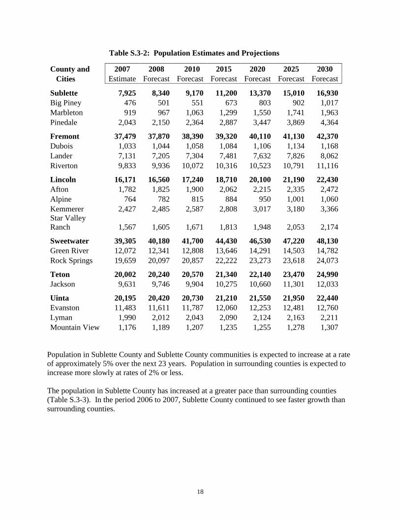
Table S.3-2: Population Estimates and Projections
County and 2007 2008 2010 2015 2020 2025 2030
Cities Estimate Forecast Forecast Forecast Forecast Forecast Forecast
Sublette 7,925 8,340 9,170 11,200 13,370 15,010 16,930
Big Piney 476 501 551 673 803 902 1,017
Marbleton 919 967 1,063 1,299 1,550 1,741 1,963
Pinedale 2,043 2,150 2,364 2,887 3,447 3,869 4,364
Fremont 37,479 37,870 38,390 39,320 40,110 41,130 42,370
Dubois 1,033 1,044 1,058 1,084 1,106 1,134 1,168
Lander 7,131 7,205 7,304 7,481 7,632 7,826 8,062
Riverton 9,833 9,936 10,072 10,316 10,523 10,791 11,116
Lincoln 16,171 16,560 17,240 18,710 20,100 21,190 22,430
Afton 1,782 1,825 1,900 2,062 2,215 2,335 2,472
Alpine 764 782 815 884 950 1,001 1,060
Kemmerer 2,427 2,485 2,587 2,808 3,017 3,180 3,366
Star Valley
Ranch 1,567 1,605 1,671 1,813 1,948 2,053 2,174
Sweetwater 39,305 40,180 41,700 44,430 46,530 47,220 48,130
Green River 12,072 12,341 12,808 13,646 14,291 14,503 14,782
Rock Springs 19,659 20,097 20,857 22,222 23,273 23,618 24,073
Teton 20,002 20,240 20,570 21,340 22,140 23,470 24,990
Jackson 9,631 9,746 9,904 10,275 10,660 11,301 12,033
Uinta 20,195 20,420 20,730 21,210 21,550 21,950 22,440
Evanston 11,483 11,611 11,787 12,060 12,253 12,481 12,760
Lyman 1,990 2,012 2,043 2,090 2,124 2,163 2,211
Mountain View 1,176 1,189 1,207 1,235 1,255 1,278 1,307
Population in Sublette County and Sublette County communities is expected to increase at a rate
of approximately 5% over the next 23 years. Population in surrounding counties is expected to
increase more slowly at rates of 2% or less.
The population in Sublette County has increased at a greater pace than surrounding counties
(Table S.3-3). In the period 2006 to 2007, Sublette County continued to see faster growth than
surrounding counties.

19
Table S.3-3: Population Growth
Population Sublette Sweetwater Lincoln Uinta Fremont Teton
Estimated 2007 7,925 39,305 16,171 20,195 37,479 20,002
Estimated 2006 7,359 38,763 16,383 20,213 37,163 19,288
Estimated 2004 6,879 38,380 15,780 20,056 36,710 18,942
2000 5,920 37,613 14,573 19,742 35,804 18,251
Percent Population Increase
2000 to 2007 34% 4% 11% 2% 5% 10%
2004 to 2007 15% 2% 2% 1% 2% 6%
2006 to 2007 8% 1% -1% 0% 1% 4%
Sublette County does not have any urbanized areas. Urbanized areas in surrounding counties are
geographically distant from the monitor with the ozone exceedance in Sublette County (the
Boulder monitor). As is described in Section 7 of this document, meteorological conditions
associated with elevated ozone episodes greatly limit the possibility of emissions transport.
Table S.3-4 shows the approximate distance to the Boulder monitor from communities with a
population greater than 9,000 in 2007. Additionally, Riverton is separated from the UGRB by
the Wind River Range. (Appendix S3 - Figure - Wyoming Population Density by Census Tract)
Table S.3-4: Distance to Boulder Monitor
(Miles, approximate)
Riverton Green River Rock Springs Jackson Evanston
73 82 80 75 118
The analysis in Section 7 of this document will demonstrate that emissions from sources outside
of the UGRB do not significantly influence ozone levels at the Boulder monitor during elevated
ozone episodes.
References:
1. http://www.census.gov/main/www/cen2000.html, U.S. Census Data.
2. http://eadiv.state.wy.us/pop/CO-07EST.htm, State of Wyoming populations statistics and
projections by county and city.
3. Appendix S.3., Population Density by Census Tract

20
SECTION 4
TRAFFIC AND COMMUTING PATTERNS
SYNOPSIS
The number of commuters into or out of Sublette County (and the UGRB) is small and does not
support adding other counties or parts of counties into the nonattainment area based on
contribution of emissions from commuters from other counties.
The percent of emissions from on-road mobile sources is small within the proposed
nonattainment area: 7% of NOx and 0.3% of VOCs. Even if this source increases, it will remain
a small percentage of total emissions.
Interstate 80, the interstate highway that is nearest to the Boulder monitor, is approximately 80
miles south of the Boulder monitor. Ozone monitors in closer vicinity to the interstate have not
shown ozone exceedances. I-80 traffic is not considered to be a significant contributor of
emissions that impact the Boulder monitor during ozone events.
ANALYSIS
Consistent with the rural character of the counties in southwest Wyoming including Sublette
County, traffic volumes are low. The Wyoming Department of Transportation’s (WYDOT)1
inventory shows traffic volume at 447,953 daily vehicle miles traveled (DVMT) for Sublette
County in 2007. WYDOT inventories are based on travel on paved roads. Table S.4-1 shows
traffic volumes for Sublette County and surrounding counties for 1994, 2004 and 2007.
Emissions from mobile sources within the UGRB are very low, as would be expected from such
low DVMTs. As shown in Table S.2-1, NOx emissions for the first quarter of 2007 are
approximately 136 tons (7% of total NOx) and VOC emissions are 79 tons (0.3%). This makes
emissions from this sector of much lower significance than is typically seen in urban
nonattainment areas.
Approximately 90% of the traffic volume in Sweetwater and Uinta Counties is interstate traffic.
Interstate 80 is located approximately 80 miles south of the Boulder monitor, the ozone monitor
that showed the exceedance. There are five ozone monitors located closer to the Interstate:
Wamsutter (~1 mile), OCI (~12 miles), South Pass (~45 miles), Murphy Ridge (~5 miles), and
Jonah (~60 miles) (See Figure S.1-1). None of the monitors located closer to the Interstate have
shown an ozone exceedance.
21
Table S.4-1: WYDOT - 2007 Traffic Surveys
Sublette Sweetwater Lincoln Uinta Fremont Teton
DVMT-2007 447,953 2,667,117 615,113 1,013,595 979,546 622,356
DVMT - interstate-
2007 2,421,684 911,916
DVMT-2004 342,034 2,473,882 564,771 944,416 892,814 600,836
DVMT-1994 229,553 1,917,738 466,753 761,626 737,863 504,904
Increase 1994 to
2007 95% 39% 32% 33% 33% 23%
Miles of roads 229.2 568.7 337.2 218.4 507.2 144.2
DVMT/mile of road 1954 4689 1824 4641 1931 4315
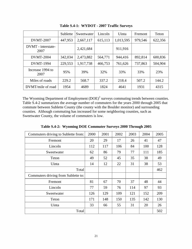
The Wyoming Department of Employment (DOE)2 surveys commuting trends between counties.
Table S.4-2 summarizes the average number of commuters for the years 2000 through 2005 that
commute between Sublette County (the county with the Boulder monitor) and surrounding
counties. Although commuting has increased for some neighboring counties, such as
Sweetwater County, the volume of commuters is low.
Table S.4-2: Wyoming DOE Commuter Surveys 2000 Through 2005
Commuters driving to Sublette from: 2000 2001 2002 2003 2004 2005
Fremont 20 29 17 26 41 47
Lincoln 112 117 106 84 100 128
Sweetwater 62 86 79 77 111 185
Teton 49 52 45 35 38 49
Uinta 14 12 22 31 38 53
Total
462
Commuters driving from Sublette to:
Fremont 81 67 70 37 48 44
Lincoln 77 59 76 114 97 93
Sweetwater 126 129 109 121 152 209
Teton 171 148 150 135 142 130
Uinta 33 66 55 31 20 26
Total
502

22
North Carolina’s Economic Development Intelligence System (EDIS)3 compiled 2000 Census
data to determine the number of commuters in Wyoming counties. Extrapolating this data to
2008, to account for only population growth, the estimated number of commuters in Sublette
County and surrounding counties is shown in Table S.4-3. Since rapid population growth in
Sublette County is biased toward the working age population, the straight extrapolation from
2000 data is likely to underestimate the number of commuters. The EDIS data indicate the
majority of commuters commute within their county of residence. The number of commuters
leaving Sublette County calculated by the Wyoming DOE correlates well with the EDIS
generated estimates of commuters leaving Sublette County.
Table S.4-3: Number of Commuters in Sublette and Surrounding Counties
Sublette Sweetwater Lincoln Uinta Fremont Teton
Estimated number of commuters in
2000* 2767 18,012 6069 8921 15,074 10,527
Estimated number of commuters in
2008 3357 18,726 7084 9114 15,761 11,811
Estimated number of 2008
commuters that stay in their county 2921 17,977 5596 7565 14,973 11,338
* 2000 Census data
Commuting patterns in Sublette County and in surrounding counties show that commuting to or
from the adjacent counties is not a major source of VMT in Sublette County. Therefore,
commuters from adjacent counties are not a significant factor in ozone generation in the
proposed nonattainment area.
Reference:
1. Appendix S.4.A, 2007 Vehicle Miles on State Highways By County
2. Appendix S.4.B, Commuting Patterns in Sublette County
3. North Carolina Department of Commerce web site.
https://edis.commerce.state.nc.us/docs/countyProfile/WY/

23
SECTION 5 GROWTH RATES AND PATTERNS
SYNOPSIS
The pace of growth in the oil and gas industry in Sublette County is significantly greater than in
surrounding counties. While population is growing in Sublette County, the county and
surrounding area is rural with a low population density. Population growth does not influence
determination of a designation area boundary in this case.
ANALYSIS
Statistical data available is broken down on a county basis. The following analysis compares
Sublette County to surrounding counties. While the recommended nonattainment area includes a
portion of Sweetwater and Lincoln counties in addition to Sublette, the trends described for
Sublette County also hold true, in general, to the recommended nonattainment area.
Population growth is described in Section 3. Sublette County population has grown at an annual
rate of approximately five percent over the last seven to ten years. Sublette County is forecast to
continue to grow at this rate for the foreseeable future. Counties surrounding Sublette have
grown at rates of less than two percent during this time period and are forecast to continue to
grow at this slower pace.
Industrial growth in Sublette County is driven by the oil and gas (O&G) industry. Table S.5-1
shows the increase in O&G production for Sublette County as shown by the number of well
completions for years 2000 through 2008. Table S.5-2 shows total well completions for 2005
through 2008 for Sublette, Sweetwater, Uinta and Lincoln counties. Sweetwater and Lincoln
counties also show an increasing trend in well completions, though to a lesser extent than in
Sublette. Teton County is not listed because it has no oil and gas production. Fremont County
is not shown because O&G production areas in Fremont County are separated from the other
counties by the Wind River Mountain Range.
Table S.5-1: Completion Report Sublette County*
(Confidential Records Are Not Listed)
2000 2001 2002 2003 2004 2005 2006 2007 2008
Distinct Gas Well
Completion Count 126 110 150 185 252 281 428 420 517
Distinct Oil Well
Completion Count 45 20 32 15 5 0 3 5 4
Total Distinct Well
Completion Count 172 131 188 202 260 287 434 434 531
*Wyoming Oil and Gas Conservation Commission (WOGCC)

24
Table S.5-2: Total Well Completions/Oil, Gas, and CBM*
(Confidential Records Are Not Listed)
2000 2001 2002 2003 2004 2005 2006 2007 2008
Sublette 172 131 188 202 260 287 434 434 531
Sweetwater 120 129 166 287 230 238 276 242 274
Lincoln 39 18 18 33 57 101 103 91 106
Uinta 19 13 3 4 18 15 20 18 14
*Wyoming Oil and Gas Conservation Commission (WOGCC)
As Figure S.5-1 shows, there have been more O&G well completions in Sublette than for the
surrounding counties. Table S.5-3 and Figure S.5-2 show the steady growth in Sublette County
O&G production since 2000.
0
100
200
300
400
500
600
2000 2001 2002 2003 2004 2005 2006 2007 2008
Figure S.5-1: Well Completions Per County
Sublette
Sweetwater
Lincoln
Uinta

25
Table: S.5-3 Sublette County Production Levels
Oil Bbls Gas Mcf Water Bbls
2008 7,666,396 1,143,614,170 22,921,983
2007 7,096,499 1,008,001,400 18,251,807
2006 5,769,581 880,855,575 13,203,000
2005 5,102,164 814,748,425 11,641,926
2004 4,705,836 731,276,509 11,812,077
2003 4,539,385 655,573,062 10,526,328
2002 4,380,011 571,000,866 13,950,895
2001 3,840,436 493,577,283 7,785,291
2000 3,345,063 448,281,668 7,364,792
Table S.5-4 shows growth in the oil and gas industry by county through the following three
measures: oil production (in barrels), gas production (in thousand cubic feet), and produced
water generation (in barrels). Growth in production of gas and water is increasing in Sublette
County and is either static or decreasing in the surrounding counties.
0.0E+00
2.0E+08
4.0E+08
6.0E+08
8.0E+08
1.0E+09
1.2E+09
2000 2001 2002 2003 2004 2005 2006 2007 2008
Figure S.5-2: Sublette County Gas Production
Mcf

26
Table S.5-4: Four County Production
Oil Bbls
Sublette Lincoln Sweetwater Uinta
2008 7,666,396 819,751 5,392,316 1,341,993
2007 7,096,499 801,807 5,738,262 1,506,562
2006 5,769,581 782,165 5,295,610 1,914,262
2005 5,102,164 762,801 4,872,531 2,246,896
Gas Mcf
2008 1,143,614,170 89,516,900 240,214,449 130,282,928
2007 1,008,001,400 89,189,164 235,687,851 128,068,870
2006 880,855,575 85,753,007 238,339,251 139,700,716
2005 814,748,425 83,579,467 222,772,057 141,490,407
Water Bbls
2008 22,921,983 1,228,058 42,026,953 3,011,981
2007 18,251,807 1,300,854 47,522,714 2,843,082
2006 13,203,000 1,375,969 49,928,115 2,641,554
2005 11,641,926 1,065,943 45,110,120 2,950,473
References:
Wyoming Oil and Gas Conservation Commission (http://wogccms.state.wy.us/)

27
SECTION 6
GEOGRAPHY/TOPOGRAPHY
SYNOPSIS
The Wind River Range, with peaks up to 13,800 feet, bounds the UGRB to the east and north;
the Wyoming Range, with peaks up to 11,300 feet, bounds the UGRB to the west.
Significant terrain influences the weather patterns throughout Southwest Wyoming. Other
terrain features such as river and stream valleys also influence local wind patterns.
Mountain-valley weather patterns in the UGRB tend to produce limited atmospheric mixing
during periods when a high pressure system is in place, setting up conditions for temperature
inversions, which are enhanced by the effect of snow cover.
ANALYSIS
Southwest Wyoming and the UGRB are within the Wyoming Basin Physiographic Province.
Topography in the UGRB is characterized by low, gently rolling hills interspersed with buttes.
Elevations range from approximately 7,000 to 7,400 feet above mean sea level (AMSL) in the
lowest portions of the UGRB. The Wind River Range, with peaks up to 13,800 feet, bounds the
UGRB to the east and north and the Wyoming Range, with peaks up to 11,300 feet, bounds the
UGRB to the west. There are also important low terrain features such as the Green River Basin
and the Great Divide Basin.
Mountain elevations decrease moving south along both the Wyoming and Wind River ranges.
Along the western boundary of the Green River Basin, in the southern part of the Wyoming
Range, the elevation decreases to about 6,900 feet above mean sea level (AMSL) with some
peaks in the 7,500 to 8,000-foot range. Moving south along the Wind River Range, the elevation
decreases to 7,800 feet at South Pass.

28
Figure S.6-1: Nonattainment area shown (blue outline) against an aerial view
of the topography in the Upper Green River Basin and adjacent areas.
The surrounding significant terrain features effectively create a bowl-like basin in the northern
portion of the Green River Basin, which greatly influences localized meteorological and
climatological patterns relative to geographical areas located outside of the UGRB. Although
difficult to quantify over the entire UGRB valley, the UGRB is roughly 900 to 1,300 meters
(3,000 to 4,300 feet) lower than the terrain features bounding the UGRB to the east and west.
Typical elevation profiles within the UGRB are illustrated in two different cut-planes (transects)
across the UGRB, as shown in Figure S.6-2.
The southern boundary of the area is defined by river and stream channels. To the east the Big
Sandy, Little Sandy and Pacific Creek drainages define the boundary and to the west the Green
River and Fontenelle Creek drainages define the boundary.

29
Figure S.6-2: Transects across the Upper Green River Basin (running north-south and
west-east) showing cross sections of the terrain; terrain elevations and distance units shown
in the transects are in meters.
Significant terrain in the UGRB has an impact on the local meteorology (wind speed, wind
direction, and atmospheric stability). In mountain-valley areas – such as the UGRB – during the
night cold air will accelerate down the valley sides (downslope winds), while during the day
warmer air will flow up the valley sides (upslope winds). At night, this can create a cold pool of
air within the UGRB that stratifies the atmosphere (inhibits mixing) since colder, denser air
exists at the surface with warmer air above. Further, at the valley floor, the wind speed is likely
to be lower than in an open plain as the roughness of the surrounding terrain tends to decrease
wind speeds at the surface. The terrain obstacles surrounding the UGRB also tend to cut-off,
block, or redirect air that might normally flow through the valley. This effect is exacerbated
Approximate South boundary
of proposed nonattainment area
Meters Meters

30
during times of calm weather, such as the passage of a high pressure system that tends to set up
conditions for strong surface-based temperature inversions.
The Wind River Range on the east and the Wyoming Range on the west provide significant
barriers to movement of ozone and ozone precursors into the area proposed for a nonattainment
area designation. Although the recommended southern boundary is not bordered by a mountain
range, the southern boundary lies along two significant drainage divides: the Fontenelle/Green
River and the Pacific/Big Sandy River. These geographic features influence air flow, although
they do not provide an absolute barrier to migration. The influence of these geographic features
on wind flows, especially during periods of low winds which are needed for ozone formation is
illustrated in Figure S.7-17. This figure shows winds generally conforming to the drainages
which establish the southern boundary of the proposed nonattainment area. The conclusions
about the southern boundary are further supported by the meteorological analyses presented in
Section 7.

31
SECTION 7
METEOROLOGY
SYNOPSIS
The unique meteorology in the UGRB of Wyoming creates conditions favorable to wintertime
ozone formation.
The meteorology within the UGRB during winter ozone episodes is much different than on non-
high ozone days in the winter, and is also much different than the regional meteorology that
exists outside of the UGRB during these wintertime high ozone episodes.
The 2008 field study data reveal that, for the days leading up to the February 19-23, 2008 ozone
episode, sustained low wind speeds measured throughout the monitoring network were
dominated by local terrain and strong surface-based inversions, which significantly limited the
opportunity for long-range transport of precursor emissions and ozone to reach the Boulder
monitor.
Minimal emissions transport and dispersion, due to the influence of localized winds (light winds)
in the UGRB characterize the February 19-23, 2008 ozone episode.
An ozone-event specific wind field was developed to more accurately simulate meteorological
conditions in the UGRB and surrounding areas, and was used to drive a trajectory model for air
parcel movement into and out of the UGRB.
Trajectory analyses were used to develop a reasonable southern boundary for the nonattainment
area.
The unique meteorological conditions in the UGRB are one of the most significant factors for
assigning this nonattainment boundary.
ANALYSIS
General
There is significant topographic relief in Wyoming which affects climate and daily temperature
variations. This is a semiarid, dry, cold, mid-continental climate regime. The area is typified by
dry windy conditions, with limited rainfall and long, cold winters. July and August are generally
the hottest months of the year, while December and January are the coldest. Pinedale’s mean
temperature in January is 12.5°F with a mean of 60°F in July (Western Regional Climate Center,
2009). The high elevation and dry air contribute to a wide variation between daily minimum and
maximum temperatures. At Pinedale, the total annual average precipitation is about 10.9 inches,
and an average of 61 inches of snow falls during the year.
Strong winds are common in Wyoming, especially in the south. Wind velocity can be
attributable, in part, to the prevailing westerly winds being funneled through the Rock Mountains
at a low point in the Continental Divide.
The meteorological conditions conducive to the formation of high ozone levels in the UGRB
during the winter and early spring are characterized by:
- A stable atmosphere, characterized by light low-level winds

32
- Clear or mostly sunny skies
- Low mixing heights or capping inversions
- Extensive snow cover
- Low temperatures
The above conditions take some time to develop (at least 48 hours after a storm frontal passage),
and occur during periods when the synoptic weather is dominated by high pressure over the
western Rockies.
Looking at the meteorological conditions in the UGRB, elevated ozone episodes in 2005, 2006
and 2008 were associated with strong temperature inversions and light low-level winds. This
was the case during the February 19-23, 2008 ozone episode, in which the highest ozone
concentrations monitored to date in the UGRB were recorded at the Boulder monitor. Because
these meteorological conditions are common to all of the high ozone episodes in the UGRB
observed to date, the ozone episode of February 19-23, 2008, a 5-day period marking the longest
consecutive ozone episode observed, is considered to be representative of other ozone episodes.
This particular 5-day ozone episode is the primary focus of this section on meteorological
influences and wintertime high ozone.
Winter Ozone Field Studies
After elevated ozone levels were monitored in the winter of 2005 and 2006; the AQD initiated
intensive field studies to collect meteorological and ambient data in the first quarter of 2007,
2008, and 2009 throughout the Green River Basin to better understand the relationships between
winter meteorological conditions and high ozone levels versus low ozone levels. In spite of
careful planning to record data, the winter of 2007 did not produce conditions conducive to the
formation of ozone. In contrast, the winter of 2008 provided a significant amount of data on
ozone formation since there were several high ozone episodes. A map showing the monitoring
sites employed in the 2008 field study and regional terrain features in the 2008 study area is
shown in Figure S.7-1. The entire data set and reports on the winter studies completed to date
are available on the WDEQ/AQD website (http://deq.state.wy.us/aqd/Monitoring%20Data.asp).
AQD has continued field studies into 2009, but those results will not be available until later in
2009.
During January and the beginning of February 2008, the study area was under the influence of a
series of weak to moderately strong synoptic disturbances that migrated from the Gulf of Alaska,
across the Pacific Northwest and southern British Columbia and the northern Great Basin and
into the Northern Rockies. These weather features generally moved rapidly through southwest
Wyoming as they migrated along a belt of strong westerly to northwesterly winds aloft that were
associated with a persistent high pressure ridge located over the eastern Pacific, off California.
In addition, a number of deep Pacific troughs moved across the area earlier in the winter and into
the first half of January. The end result of all this activity was the deposit of substantial snow
cover in southwestern Wyoming, including the UGRB, which was to remain in place through the
rest of the winter. After mid-February, the eastern Pacific ridge exhibited a tendency to extend
or migrate into the interior west until it finally moved directly over southwest Wyoming by
February 20, 2008.
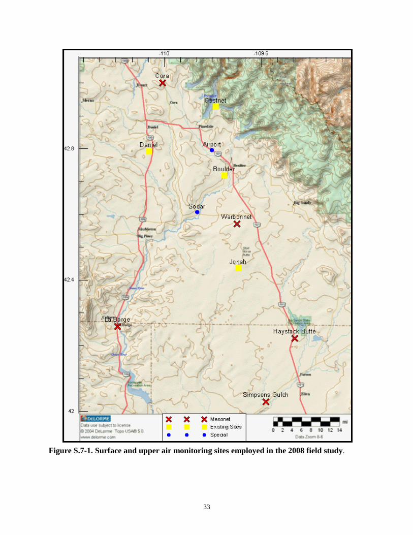
33
Figure S.7-1. Surface and upper air monitoring sites employed in the 2008 field study.

34
Comparison of 2007 and 2008 Field Study Observations
Snow Cover and Sunlight
Comparison of meteorological conditions in 2008 with those prevailing during the 2007 field
study revealed that one of the key differences was the extensive snow cover in 2008 which was
not present during 2007. Snow cover appears to be a key ingredient in winter ozone
development, specifically, fresh snow, which results in higher surface albedo, perhaps as great as
0.9. The increased surface albedo results in greater actinic flux and therefore elevated NO2
photolysis rates. The elevated photolysis rate due to the high (snow cover driven) albedo is
likely greater than the photolysis rate in the UGRB in the summer months.
During the 2007 field study, although there were extended periods when synoptic-scale
meteorological conditions were conducive to poor horizontal dispersion, the lack of snow cover
and subsequent lower UV albedo reduced the amount of UV radiation available for photolysis
and associated ozone production. In addition, the 2007 and 2008 field studies suggest that the
sensible and radiative heat flux impacts of the snow cover enhance low-level atmospheric
stability, substantially reducing vertical mixing during most or all of the daylight hours.
Low Wind Speeds
Stable, stagnant weather conditions occurred in southwest Wyoming during the period from
February 18 through 22, 2008. The main synoptic feature responsible for this was a strong
Pacific high pressure ridge that slowly migrated across the western United States. This period
was dominated by low wind speeds in the boundary layer, which reduced pollutant transport and
dispersion. This effect is shown in Figure S.7-2 where ozone concentrations and wind speeds are
plotted for the Boulder monitor for February and March of 2008.
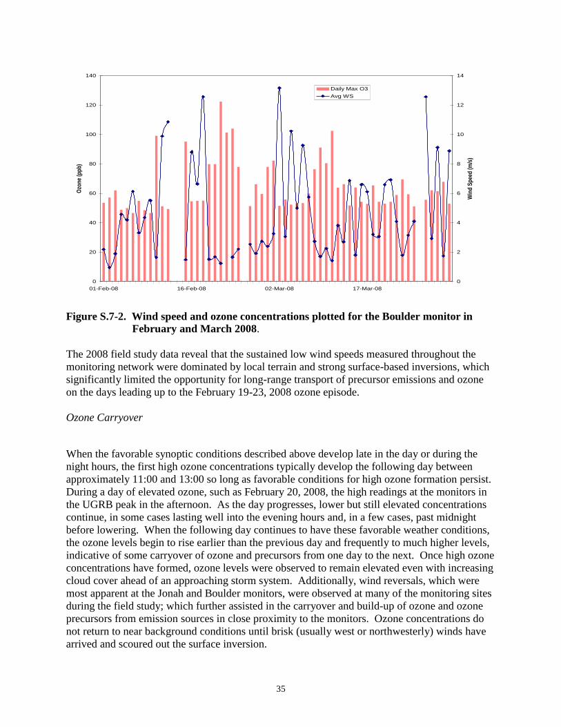
35
Figure S.7-2. Wind speed and ozone concentrations plotted for the Boulder monitor in
February and March 2008.
The 2008 field study data reveal that the sustained low wind speeds measured throughout the
monitoring network were dominated by local terrain and strong surface-based inversions, which
significantly limited the opportunity for long-range transport of precursor emissions and ozone
on the days leading up to the February 19-23, 2008 ozone episode.
Ozone Carryover
When the favorable synoptic conditions described above develop late in the day or during the
night hours, the first high ozone concentrations typically develop the following day between
approximately 11:00 and 13:00 so long as favorable conditions for high ozone formation persist.
During a day of elevated ozone, such as February 20, 2008, the high readings at the monitors in
the UGRB peak in the afternoon. As the day progresses, lower but still elevated concentrations
continue, in some cases lasting well into the evening hours and, in a few cases, past midnight
before lowering. When the following day continues to have these favorable weather conditions,
the ozone levels begin to rise earlier than the previous day and frequently to much higher levels,
indicative of some carryover of ozone and precursors from one day to the next. Once high ozone
concentrations have formed, ozone levels were observed to remain elevated even with increasing
cloud cover ahead of an approaching storm system. Additionally, wind reversals, which were
most apparent at the Jonah and Boulder monitors, were observed at many of the monitoring sites
during the field study; which further assisted in the carryover and build-up of ozone and ozone
precursors from emission sources in close proximity to the monitors. Ozone concentrations do
not return to near background conditions until brisk (usually west or northwesterly) winds have
arrived and scoured out the surface inversion.
0
20
40
60
80
100
120
140
01-Feb-08 16-Feb-08 02-Mar-08 17-Mar-08
Ozo
ne
(pp
b)
0
2
4
6
8
10
12
14
Win
d S
pee
d (
m/s
)
Daily Max O3
Avg WS

36
Atmospheric Mixing
The observed weather patterns in the 2007 field study showed that the winter storm systems
generally did not provide a strong push of cold air and did not produce much precipitation in the
project area, but did allow strong wind speeds aloft with considerable mixing of the atmosphere.
Specifically, the weather conditions over the study area during February and March of 2007 were
characterized by less precipitation (including less snow depth), stronger winds aloft and much
warmer surface temperatures compared to the previous two winters. High pressure systems in
2007 tended to keep the air mass over the study area relatively well mixed and mild, which in
turn did not allow for snow accumulation and strong inversion development.
Feb. 19 – 23, 2008 Case Study Illustrating the Specific Weather Conditions Which Produce
Elevated Ozone in the Upper Green River Basin
This ozone episode is of particular interest for study, as it: 1) occurred over five days, marking
the highest 1-hour and 8-hour ozone concentrations recorded at the Boulder monitor to date, 2)
occurred during a field study Intensive Operating Period (IOP) that was in place to measure
detailed actual ambient and meteorological conditions leading up to and during this multi-day
winter ozone episode, 3) provides a high quality database of observations for several
meteorological parameters, both during IOPs and regular hourly observations during this ozone
episode, and 4) provides information which clearly shows how the topography in the Upper
Green River Basin creates different meteorological conditions within the UGRB. A summary of
the daily maximum 8-hour averaged ozone concentrations monitored at the Jonah, Boulder, and
Daniel FRM monitors during this ozone episode, as well as the day immediately preceding it, are
provided in Table S.7-1.
Date
Jonah
(ppb)
Boulder
(ppb)
Daniel
(ppb)
2/18/09 45 55 54
2/19/08 80 79 74
2/20/08 75 79 76
2/21/08 84 122 62
2/22/08 102 101 76
2/23/08 76 104 74
Table S.7-1. Summary of daily maximum 8-hour averaged ozone concentrations
monitored at the Jonah, Boulder, and Daniel monitors during February 18-23.

37
A synopsis of the particular meteorological conditions associated with the February 19-23, 2008
winter high ozone episode is provided below, describing the evolution of the meteorological
conditions that were in place during the February 19-23, 2008 ozone episode.
Synopsis of 19 – 23 February 2008 Ozone Episode
Figure S.7-3 shows the 700 millibar (mb) chart for the morning of February 19, 2008, which
shows the axis of the Pacific ridge extending north and south from the Four Corners area,
through northwestern Idaho and up into eastern British Columbia. At that time, the ridge axis
was still west of Wyoming, resulting in fairly strong northwesterly gradient flow (winds blowing
from the northwest along the isobars) just above ground level in southwest Wyoming. With
clear skies accompanying the approaching ridge, and a good snow cover at the surface, a capping
inversion formed overnight and persisted throughout the next day in the UGRB. However, the
strong winds above the stable layer, along with mixing heights on the order of several hundred
meters, transferred sufficient momentum downward, allowing these northwest winds to mix
down to the surface during the day resulting in predominant northwesterly wind patterns within
the UGRB.
Figure S.7-3. Constant pressure map for 700 mb, 02/19/08 (1200 UTC) [(5 am LST)].

38
The high pressure ridge continued to progress slowly eastward during February 20th
resulting in
the central axis pushing into southwestern Wyoming by the middle of the day. As a result, a
capping low-level inversion was observed throughout the day, and a weakened northwest
gradient wind flow allowed the establishment of local valley flow patterns in the area. Local
valley flow patterns are characterized by light variable winds with pronounced down slope winds
at night. A weak storm system that moved out of California and across the southern Great Basin
during February 20th
forced some broken high cloudiness over southwestern Wyoming during
the afternoon, but the clouds failed to curtail ozone production in the area, based on monitored
data.
Figure S.7-4 shows the 700 mb chart for the evening of February 21, 2008. Although the high
pressure ridge had weakened by the afternoon of February 21st, it had also flattened and the
central ridge axis was over southwestern Wyoming through the entire day. The resulting light
wind situation, characterized by low wind speeds and significantly reduced air flow movement
within the UGRB, enabled the strongest ozone production seen to date in Sublette County.
Figure S.7-4. Constant pressure map - 700 mb, 02/22/08 (0000 UTC) [02/21/08 (5 pmLST)].

39
On February 21, 2008, the low level inversion stayed intact through the entire daylight period,
keeping ground level emissions trapped near the surface. With the very light and variable winds
above the inversion (see Figure S.7-10) localized wind flow patterns near the ground level
developed during the day allowing emissions to transport along those pathways (see Figure S.7-6
and Figure S.7-7). The height of the 700 mb pressure surface during the day was around 3,020
meters (MSL), the temperature averaged about -6° C, and the wind speeds were less than 5
knots. The height of the 500 mb pressure surface averaged around 5,550 meters (MSL) and the
wind speeds at that height were around 15 knots.
The high pressure ridge continued to weaken during February 22, 2008, while a shortwave low
pressure trough approached southwestern Wyoming from the northwest. Skies became mostly
cloudy during the morning hours and light precipitation spread over the area later in the
afternoon; the low level inversion stayed intact well into the afternoon, and ozone concentrations
remained high during most of the day. It was anticipated that the stable layer would be mixed-
out by the trough by early morning the next day and trapped emissions would be dispersed.
Instead, the late arrival of the trough allowed one more day of high ozone concentrations.
Description of Surface Wind Data
With the addition of the temporary mesonet monitoring sites to the existing permanent
meteorological monitoring stations in the 2007 and 2008 field studies, a fairly detailed picture of
wind flow patterns within the UGRB was obtained, revealing that the wind flow patterns were
distinctly different throughout the northern and southern portions of southwest Wyoming. A
composite map of wind rose plots generated from meteorological data collected throughout
southwest Wyoming during the time period 18 – 22, February 2008 is provided in Figure S.7-5.
As can be seen in Figure S.7-5, the wind patterns in the northern portion of Sublette County
reflect the prevailing northwest winds typical of this area during most of the year. However, this
moderately strong, organized northwest flow does not extend to the southern monitoring sites
(Haystack Butte and Simpsons Gulch). Monitoring sites located in Sweetwater, Lincoln and
Uinta Counties experienced a generally westerly wind flow, which was also a characteristic of
the prevailing flows noted during the 2007 field study at those monitoring sites. Additionally,
during the afternoon, winds reversed at some monitoring sites in the UGRB, shifting from the
northwest to the southeast; this mid-day flow reversal is typical of high ozone days in the UGRB,
and is thought to be causing recirculation of pollutants within the UGRB.

40
Figure S.7-5. Composite wind rose map for February 18 – 22, 2008 at monitoring sites
located throughout Southwest Wyoming.
Wind vector fields were also examined spatially to gain an understanding of flow patterns in the
field study area. Winds on a typical ozone episode day (February 20th
), and on the day with the
highest 8-hour ozone concentration recorded at the Boulder monitoring site (February 21st) are
shown in Figure S.7-6 and Figure S.7-7.

41
Figure S.7-6. Time-series showing February 20, 2008 hourly wind vectors for monitors
used in 2008 field study monitoring network.
As shown in Figure S.7-6, winds in the UGRB are generally out of the northwest in the morning
until about mid-day, at which point the flow has reversed with southeasterly winds, or at least
southerly component winds are observed at most sites. This continues through the afternoon
until 18:00 MST at which time the flow begins to switch back to the northwest, and by 6:00
MST the following morning, winds are northwest or northeast at nearly all of the monitoring
sites. The switch from an overnight flow consisting of generally northwesterly or down slope
winds, which last until approximately mid-day before reversing to a generally southeasterly wind
flow pattern during the afternoon, was repeated on many of the 2008 ozone episode days.
N

42
Figure S.7-7. Time-series showing February 21, 2008 hourly wind vectors for monitors
used in 2008 field study monitoring network.
As shown in Figure S.7-7, winds on February 20th
and 21st were generally light with variable
directions throughout the monitoring network. There were two notable exceptions. After
midnight, there was a general light northwest flow suggestive of a regional drainage pattern as
colder, heavier air from the higher elevations flows downhill.
Generally stronger winds were measured at Jonah in the forenoon hours relative to the other sites
in the network; this effect is also sometimes seen at Daniel and is likely due at least in part to the
fact that winds at these two sites are measured on a standard 10 meter tower whereas the other
sites made use of 3 meter high tripod mounted anemometers. During the afternoon, winds
reversed at some sites, shifting to the southeast. This mid-day flow reversal is typical of high
ozone days in the UGRB. On February 20, 2008, peak 8-hr ozone concentrations in the 70-85
ppb range were measured at sites throughout the study area; on February 21, 2008, the Boulder
monitor recorded a 122 ppb 8-hr average ozone concentration. High ozone continued on
February 22, 2008 with the Jonah monitor recording a daily maximum 8-hour average ozone
concentration of 102 ppb. Minimal emissions transport and dispersion, due to the light winds in
the UGRB, were characteristic throughout the February 19-23, 2008 ozone episode.
The South Daniel FRM monitor which is in the northwest portion of the recommended
nonattainment area is typically upwind of local precursor sources and the Boulder monitor. On
February 20 ambient nitrogen dioxide (NO2) concentrations at the Daniel monitor were
essentially equal to zero (0) ppb for all 24 hours; very low concentrations of VOCs were also
measured in the VOC canister samples collected at Daniel on this day. Nearly identical values
N

43
were observed at the Daniel monitor and in the Daniel VOC canister samples obtained
throughout the ozone episode (February 19-23, 2008); this was also the case during all three
IOPs. The canister samples collected at the Daniel monitor in the 2007 field study also showed
consistently low VOC concentrations. Additionally, monitored NOx concentrations recorded at
Daniel have been very low since this site began operation nearly four years ago; the VOC
canister data and the NOx monitoring conducted at Daniel clearly indicate the air coming into
this area has low ozone precursor concentrations. Additionally, based on the 2008 field study
data at the Daniel monitor, background ozone concentrations during the winter are typically in
the 50 - 60 ppb range. Daily maximum 8-hour ozone concentrations at the Daniel monitoring
site during the February 19-23, 2008 ozone episode ranged between 62-76 ppb.
One view of the surface wind direction-ozone relationship is shown on Figure S.7-8, which
presents a wind rose using measurements from the Boulder monitoring site. This diagram is
constructed using the daily peak 8-hr ozone level and 15:00 MST hourly averaged winds. These
results show that high ozone levels were associated with afternoon winds from a variety of
directions, reflecting the “light and variable” nature of the surface layer winds when the
monitored 8-hour ozone levels were above 75 ppb, as opposed to 8-hour ozone concentrations
that were less than 75 ppb, which tend to be associated with persistent higher wind speeds and
the predominant northwest flow direction along the valley axis.
Figure S.7-8. Wind roses based on 15:00 (MST) data from the Boulder site for days with
maximum 8-hour average ozone a) greater than 74 ppb (left) and b) less than
75 ppb (right).
44
Description of Conditions Aloft
A multi-level SODAR was operated continuously at a location approximately 3 miles southwest
of the Boulder monitoring site during the 2008 field study. The SODAR provided two types of
data: 1) vertical profiles of wind speed and wind direction at 10-meter increments up to 250
meters above ground level, and 2) information which allows an estimation of mixing height
(mixed layer depth). The regular hourly observations during the 2008 field study were
supplemented with high resolution measurements of vertical wind speed, wind direction, and
temperatures during the IOPs. The hourly meteorological data capture rate was excellent.
Comparing the measured wind data with peak 8-hour ozone concentrations at Boulder, a strong
correlation between ozone concentrations and low mixed layer average wind speeds is evident.
Looking at SODAR data on the afternoon of February 21, 2008, a day when 8-hour ozone
concentrations above 75 ppb were noted throughout the field study area, reveals a top to the
mixing layer at about 100 meters above ground level (AGL) representing a very shallow layer
trapping ozone precursors and other pollutants in high concentrations near the surface.
Similar vertical profiles (soundings) and boundary layer development were measured by balloon-
borne observations (ozone measurements, temperature, relative humidity and winds) on each of
the high ozone days. Stable atmospheric conditions prevailed, and were characterized by strong
low-level temperature inversions with very shallow mixing heights and light boundary-layer
winds. Peak ozone concentrations were often observed somewhat above the surface but still
within the stable inversion layer. As shown in Figure S.7-9, at low mixing heights (below 100
meters), the highest values of ozone were observed. Table S.7-2 provides a summary of the days
with low-level capping inversions, and the measurements obtained, including the date and time
of each balloon launch, the ground temperature and maximum inversion temperature
(temperature at top of inversion layer), the difference between the maximum inversion
temperature and the ground temperature (inversion layer Delta T), which reflects the strength of
the temperature inversion. Note the highest inversion layer temperature measured is 14.5 (oC)
and occurs on February 19th
.

45
Launch Launch Time Ground Temp Max Inversion Temp Inversion Layer ΔT Inversion Height
Date (MST) (oC) (
oC) (
oC) (meters AGL)
2/18/08 11:00 -3.8 -3.2 0.6 150
2/18/08 16:00 -1.8 -1.7 0.1 47
2/19/08 7:00 -14.8 -0.3 14.5 489
2/19/08 1100 -8.1 1.3 9.4 442
2/19/08 13:00 -5.3 2.2 7.5 403
2/19/08 16:00 -4.5 1.8 6.3 445
2/20/08 7:00 -13.6 -2.4 11.2 398
2/20/08 1100 -13.9 -2.0 11.9 342
2/20/08 13:00 -7.7 -3.2 4.5 449
2/20/08 16:00 -5.4 -2.3 3.1 543
2/21/08 7:00 -17.4 -4.0 13.4 500
2/21/08 1100 -7.9 -3.0 4.9 405
2/21/08 13:00 -3.4 -2.6 0.8 373
2/21/08 16:00 -5.7 -2.9 2.8 494
2/27/08 8:00 -9.7 -1.4 8.3 670
2/27/08 1100 -5.4 0.1 5.5 711
2/27/08 13:00 -2.3 1.0 3.3 608
2/27/08 16:00 -1.2 0.7 1.9 527
2/28/08 8:00 -8.6 -2.3 6.3 149
2/28/08 1100 -1.4 -2.4 -1.0 265
2/28/08 13:00 1.8 0.0 -1.8 91
2/28/08 17:00 0.5 1.0 0.5 190
2/29/08 8:47 -6.2 -2.5 3.7 460
2/29/08 1100 -8.9 -0.3 8.6 396
2/29/08 13:00 -1.4 0.3 1.7 314
2/29/08 16:00 -0.3 1.5 1.8 470
3/10/08 8:00 -12.2 -5.8 6.4 470
3/10/08 1100 -7.6 -5.0 2.6 480
3/10/08 14:00 -1.6 -2.1 -0.5 312
3/10/08 17:00 -1.3 -2.0 -0.7 705
3/11/08 8:00 -13.1 1.3 14.4 373
3/11/08 1100 -2.4 1.5 3.9 312
3/11/08 13:00 2.1 2.0 -0.1 252
3/11/08 17:00 0.5 1.2 0.7 236
3/12/08 8:00 -9.3 -2.1 7.2 142
3/12/08 1100 2.3 2.5 0.2 90
3/12/08 15:00 3.5 -0.3 -3.8 261
Table S.7-2. Summary of low-level temperature measurements, and related data on
inversion strength.

46
Figure S.7-9. SODAR-reported mixing height versus peak daily 8-hour ozone
concentrations at Boulder. Measurements limited to below approximately
250 meters above ground level (AGL).
Soundings taken in the forenoon and afternoon of February 21, 2008 are shown in Figure S.7-10.
Profiles for ozone (black line), temperature (red line), dew point temperature (dashed blue line)
and winds (vectors) are plotted as functions of height above the ground elevation of the balloon
launch site. A strong low-level inversion was present up to 2,500 meters-msl (~ 400 meters-agl)
with a maximum temperature at the top of the inversion of -2.9 oC, several degrees warmer than
the temperature at the surface. Boundary-layer winds in the forenoon were light from the west
when ozone levels were ~50 ppb, before becoming southeast in the afternoon.
Figure S.7-10 shows the inversion is setting up in the morning of February 21, 2008, and that the
inversion persisted through daylight hours, resulting in high ozone concentrations beneath the
inversion. Figure S.7-10 also shows that at 11:00 (MST) ozone concentrations were ~ 50 ppb
below the inversion height of 2,500 meters (MSL) which is shown by the green circle (left pane)
towards the bottom of Figure S.7-10; measured ozone levels above the inversion layer were also
generally ~ 50 ppb.
Normally, some vertical mixing of the air would exist, as the temperature aloft begins to fall off
with increasing height above ground; however, the strong surface-based inversion persists to
4:00 pm, effectively inhibiting vertical mixing. A shallow layer of high ozone (> 110 ppb) was
present in the afternoon (16:00 MST) sounding, which is shown by the green oval (right pane)
towards the bottom of Figure S.7-10. Ozone concentrations decrease rapidly with height below
the inversion; ozone levels above the inversion are about 50 ppb. Note that the vertical wind
shear measured at the top of the inversion layer height above ground (wind arrows on the right
side of graphs) attest to the complete decoupling of the boundary layer air from layers aloft.

47
Figure S.7-10. February 21, 2008 balloon-borne soundings; Sounding at 11:00 (MST) (left);
Sounding at 16:00 (MST) (right).
Tools to Evaluate Air Parcel Transport: HYSPLIT vs. AQplot Back Trajectory Analyses
Trajectory analyses were used to determine possible air parcel transport into the UGRB during
February 20, 2008, as a means of evaluating possible precursor emissions and ozone transport in
the UGRB and at the Boulder and Jonah monitors.
The HYSPLIT (HYbrid Single-Particle LaGrangian Integrated Trajectory) model is a trajectory
model that is used for computing simple air parcel trajectories. HYSPLIT can use meteorological
data from several archived meteorological modeling databases, including the NCEP Eta Data
Assimilation System (EDAS), which is based on a 40 kilometer resolution data (2004-present).
However, 40 kilometer (km) data may not provide sufficient resolution to resolve the significant
terrain features that influence the wind flow patterns in the UGRB. The result of using such low
resolution data to represent the terrain features in and surrounding the UGRB will be that the
modeled terrain will be much smoother, and will not match the actual terrain (see Figure S.7-11).
This will affect the wind trajectory analysis because the roughness of the terrain as well as terrain
blocking and channeling effects may not be well represented, which would otherwise influence
the wind speeds and the trajectory path lengths. In very complex terrain, such as in the UGRB,
the HYSPLIT model trajectories may not be very accurate unless the local wind flow patterns are
being driven by the large-scale synoptic conditions (e.g., strong winds).

48
Figure S.7-11. A comparison of the local terrain features at 1 km and 40 km resolution,
respectively, and the resulting “smoothed” terrain as shown in the 40 km 3-
D topographic plot.

49
Figure S.7-12 shows a similar comparison of the local terrain features at 1 km and 40 km
resolution as depicted in the 2-dimensional contour plots. Note the terrain features in the bottom
pane are much less resolved (less terrain detail and decreased roughness) than those terrain
features as shown in the top pane.
Figure S.7-12. A comparison of the local terrain features at 1 km and 40 km resolution,
respectively, as depicted in the 2-D contour plots.

50
While the trajectory model is a useful tool in assessing approximate air parcel movement, and
can be used to better understand potential pathways for pollutants moving within and into and
out of the UGRB, trajectories are a highly simplified representation of the complex, two- and
three-dimensional transport and turbulent diffusion processes that move pollutants from place to
place. Thus, a particular trajectory path is subject to uncertainty and should not be interpreted as
an exact representation of actual pollutant transport. Generally, the longer an air mass is tracked
forward or backward in time, the more uncertain is its position (Kuo et al., 1985; Rolph and
Draxler, 1990; Kahl and Samson, 1986).
Additionally, the trajectory model error is a function of the complexity of the meteorological
scenario under study. In this analysis, the strong surface-based inversion layer in place on
February 19-22, 2008 results in a decoupling of the upper air layers (above the inversion layer)
and the lower air layers (below the inversion) and winds in the upper and lower layers will at
times blow in different directions at different speeds. Winds are light and variable in the lower
layer, adding to the complexity of the situation. This very complex meteorological scenario is
difficult to represent accurately in a trajectory model.
AQD ran a comparison of 12-hour back trajectories from the Jonah and Boulder monitoring
sites, using the HYSPLIT model with the EDAS 40 kilometer meteorological data, and AQplot,
(a 2-dimensional trajectory model) using actual meteorological data from the Jonah and Boulder
monitoring sites, respectively. This comparison shows that much different back trajectories are
produced by these two models, as shown in Figures S.7-13 and S.7-14. The 2-dimensional
trajectory model (AQplot), used in these analyses, was developed by the Texas Commission on
Environmental Quality.
Additional trajectory analyses using a 3-D trajectory model are discussed in the next section.
However, for this particular comparison, a 2-D trajectory model is an acceptable model to assess
trajectories near the monitoring sites because the surface winds in the UGRB under these
episodic winter conditions have been effectively decoupled from the upper air layers. The
amount of vertical air movement is limited due to the capping inversion in place – in other
words, the movement of air parcels below the inversion is not influenced by winds above the
inversion, and there is little vertical mixing of air near the ground. Monitoring data of the
localized meteorological patterns in the proposed nonattainment area boundary show that under
these episodic conditions, the wind patterns are 2-dimensional, and the use of the 2-D AQplot
trajectory model for this particular application is reasonable under these winter meteorological
conditions (inversion, low mixing height, and stable atmosphere) as the air parcel trajectories
start off and tend to stay close to the ground.
As shown in Figures S.7-13 and S.7-14, the resulting short trajectories never get very far away
from the monitor site; considering the short duration of the trajectory analysis, less interpolation
error would be expected. The HYSPLIT model does not consider the wind influences as
measured in the 2008 field study surface monitoring network; the AQplot local-scale back
trajectories are a more accurate depiction of what is going on because of the input of local data.

51
Figure S.7-13. Comparison of HYSPLIT (red) and AQplot (pink) 12-hour back
trajectories from the Boulder monitoring site on February 20, 2008.
Figure S.7-14. Comparison of HYSPLIT (red) and AQplot (green) 12-hour back
trajectories from the Jonah monitoring site on February 20, 2008.
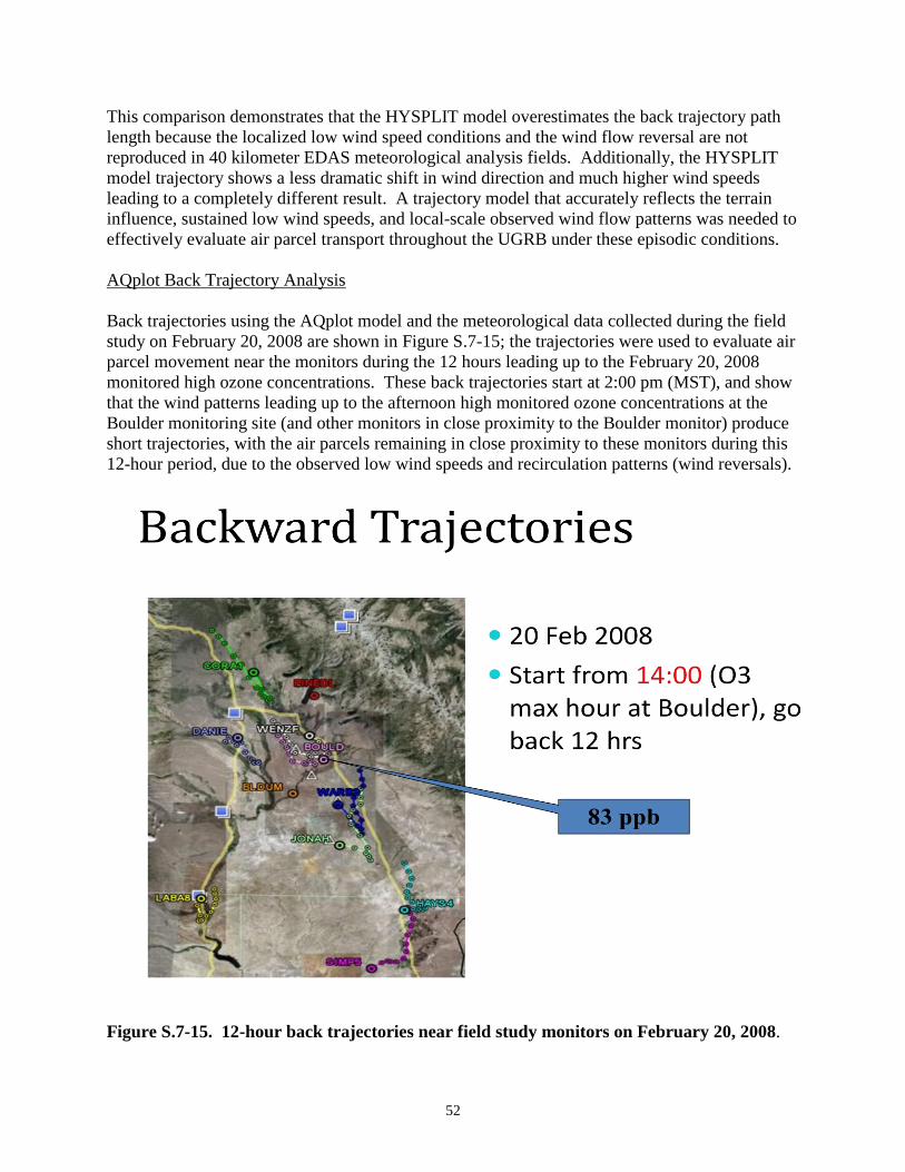
52
This comparison demonstrates that the HYSPLIT model overestimates the back trajectory path
length because the localized low wind speed conditions and the wind flow reversal are not
reproduced in 40 kilometer EDAS meteorological analysis fields. Additionally, the HYSPLIT
model trajectory shows a less dramatic shift in wind direction and much higher wind speeds
leading to a completely different result. A trajectory model that accurately reflects the terrain
influence, sustained low wind speeds, and local-scale observed wind flow patterns was needed to
effectively evaluate air parcel transport throughout the UGRB under these episodic conditions.
AQplot Back Trajectory Analysis
Back trajectories using the AQplot model and the meteorological data collected during the field
study on February 20, 2008 are shown in Figure S.7-15; the trajectories were used to evaluate air
parcel movement near the monitors during the 12 hours leading up to the February 20, 2008
monitored high ozone concentrations. These back trajectories start at 2:00 pm (MST), and show
that the wind patterns leading up to the afternoon high monitored ozone concentrations at the
Boulder monitoring site (and other monitors in close proximity to the Boulder monitor) produce
short trajectories, with the air parcels remaining in close proximity to these monitors during this
12-hour period, due to the observed low wind speeds and recirculation patterns (wind reversals).
Figure S.7-15. 12-hour back trajectories near field study monitors on February 20, 2008.

53
Due to the complexity of the winds in the UGRB during February 19-23, 2008, including the
significant terrain-dominated effects on localized winds, stable conditions, and wind flow
reversals, as discussed, and the terrain-dominated regional meteorology outside of the UGRB, a
high resolution 3-dimensional (3-D) wind field was needed that could correctly reproduce:
1) Shallow inversions and near-field wind flow patterns as measured at the SODAR, which
is near the Boulder monitor; and
2) Regional-scale wind flow patterns.
This particular wind field would be utilized in conjunction with a full 3-D trajectory model to
evaluate:
1) Air parcel movement in the study area;
2) Influences from the surrounding regional terrain on air parcel movement;
3) Air parcel inflow (ozone or precursor emissions transport) into Sublette County on the
days leading up to and during the February 19-23, 2008 ozone episode.
AQD contracted out the development of a 3-D CALMET wind field to evaluate the above, which
is discussed in the following section.
CalDESK Trajectory Analysis
AQD developed a high resolution (spatial and temporal) 3-dimensional wind field that uses the
National Center for Environmental Prediction (NCEP) Rapid Update Cycle (RUC) model at 20
kilometer resolution, coupled with the high resolution observational database of surface and
upper air meteorological data measurements obtained during the 2008 field study. It should be
noted that the terrain elevation data used in this wind field is based on much higher terrain
resolution than is currently used in the HYSPLIT model. The RUC and field meteorological data
were processed through the CALMET diagnostic wind model to generate a 1 kilometer gridded
wind field, using high resolution terrain and land use/land cover data, and actual observations of
daily snow cover to account for actual snow cover (and albedo effects) within the CALMET
domain. The complexity of the terrain, as represented in this 3-dimensional (3-D) CALMET
wind field in shown in Figure S.7-16.
This CALMET wind field was developed to evaluate the ozone episode-specific meteorology
associated with the February 18-23, 2008 ozone episode. The CALMET domain was set up
using the same meteorological modeling domain (464 km x 400 km) developed for the
Southwest Wyoming Technical Air Forum (SWWYTAF) modeling analyses (1999), with
increased vertical resolution to total 14 vertical layers; the lower layers having small vertical
depths in order to better resolve complex flow patterns and temperature inversions near the
surface.
Figure S.7-17 provides a snapshot of the wind field based on the winds at 4:00 am (MST) on
February 20, 2008, and shows the complexity of the terrain surrounding the UGRB is very well
represented in the CALMET wind field. The wind field captures the strong terrain-dominated
down slope winds during the early morning hours, and the strong channeling and drainage
effects which are exhibited throughout the UGRB – CALMET “sees” the influence of the terrain.

54
55
The 3-D CALMET wind field accurately depicts meteorological conditions in the UGRB and
surrounding area. A detailed report discussing the development of the CALMET wind field and
the validation of the wind field compared to observations, entitled, “Upper Green River Winter
Ozone Study: CALMET Database Development Phase I” will be posted on the DEQ web site
and will be sent under separate cover to EPA shortly. Validation of this wind field has shown
that the local-scale observed meteorological conditions are being reproduced:
Temperature lapse rates associated with inversion conditions and low mixing heights
Wind speeds and wind reversals
Duration of down slope winds, which last until approximately mid-day before reversing
to a generally southeasterly wind flow pattern
The trajectory analyses using this wind field lead to the conclusion that regional transport
is insignificant, and local-scale precursor emissions transport is the dominant means of
precursor transport during the high ozone periods. The trajectory analyses that follow
were a key factor in selection of an appropriate southern boundary of the nonattainment
area. The trajectory analyses demonstrate that the proposed southern boundary of the
nonattainment area is reasonable, and that there is no significant contribution of ozone or
ozone precursors from areas or sources outside the proposed nonattainment area during
elevated ozone events.
Specific Examples of Trajectory Analyses Using CalDESK
Based on this wind field, AQD used the CalDESK visualization software to run forward
trajectory analyses to evaluate air parcel transport into and out of the UGRB, specifically with
respect to air parcels from large stationary sources (power plants and Trona plants) located to the
south of the UGRB, and to evaluate the southern extent of air parcel inflow into the UGRB. A
series of CalDESK forward trajectory analyses follow, along with a brief discussion of the
resulting trajectories generated by CalDESK during February 18-23, 2008. CalDESK Forward
Trajectory Analyses (FTA) for February 18, 2008 are shown in Figures S.7-18 through S.7-22.
NOTE: Trajectory figures (Figures S.7-18 through S.7- 49) are being updated to show the
proposed nonattainment area boundary. Those figures will be available shortly. AQD will send
those figure to EPA as replacement pages.
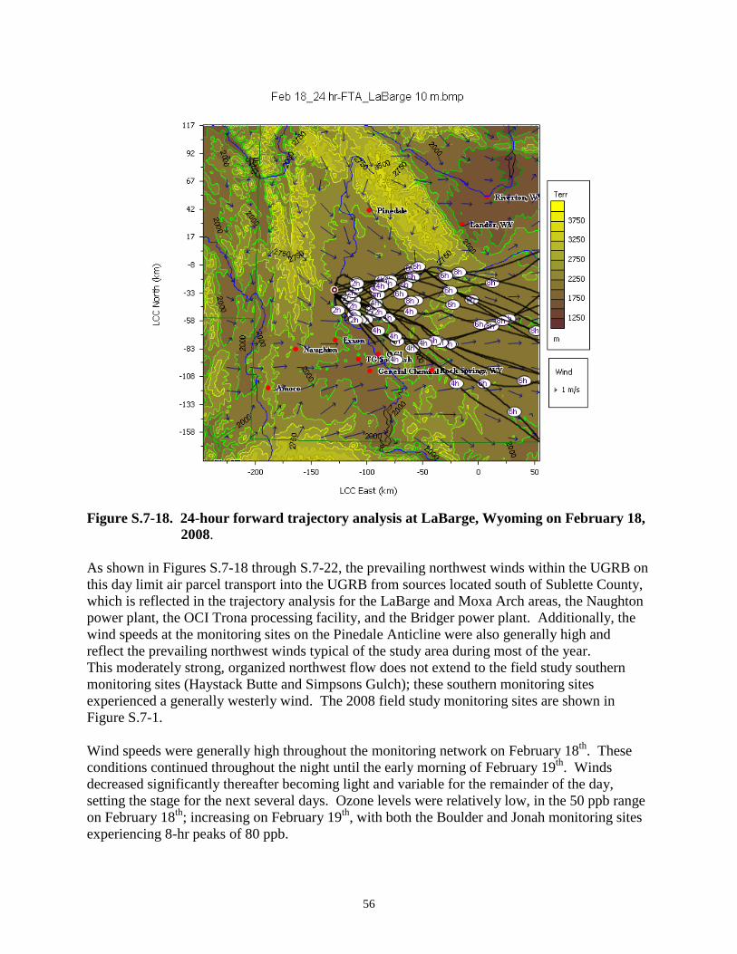
56
Figure S.7-18. 24-hour forward trajectory analysis at LaBarge, Wyoming on February 18,
2008.
As shown in Figures S.7-18 through S.7-22, the prevailing northwest winds within the UGRB on
this day limit air parcel transport into the UGRB from sources located south of Sublette County,
which is reflected in the trajectory analysis for the LaBarge and Moxa Arch areas, the Naughton
power plant, the OCI Trona processing facility, and the Bridger power plant. Additionally, the
wind speeds at the monitoring sites on the Pinedale Anticline were also generally high and
reflect the prevailing northwest winds typical of the study area during most of the year.
This moderately strong, organized northwest flow does not extend to the field study southern
monitoring sites (Haystack Butte and Simpsons Gulch); these southern monitoring sites
experienced a generally westerly wind. The 2008 field study monitoring sites are shown in
Figure S.7-1.
Wind speeds were generally high throughout the monitoring network on February 18th
. These
conditions continued throughout the night until the early morning of February 19th
. Winds
decreased significantly thereafter becoming light and variable for the remainder of the day,
setting the stage for the next several days. Ozone levels were relatively low, in the 50 ppb range
on February 18th
; increasing on February 19th
, with both the Boulder and Jonah monitoring sites
experiencing 8-hr peaks of 80 ppb.

57
Figure S.7-19. 24-hour forward trajectory analysis in the Moxa Arch area on February 18,
2008.
The trajectory analysis shown in Figure S.7-19 places the initial air parcel release point in the
northern part of the Moxa Arch field. The predominant paths shown trend to the east, and there
is a slight northerly component to several of the modeled trajectories. These trajectories
generally parallel the southern boundary of the proposed nonattainment area along Pacific Creek.
While some of the trajectory paths lie within the proposed nonattainment area, none of the paths
indicate that sources within the Moxa Arch cause or contribute to elevated ozone levels within
the proposed nonattainment area.

58
Figure S.7-20. 24-hour forward trajectory analysis at Naughton power plant on February
18, 2008.
The trajectory analysis in Figure S.7-20 shows all modeled trajectories from Naughton not
entering the proposed nonattainment area.

59
Figure S.7-21. 24-hour forward trajectory analysis at OCI Trona plant on February 18,
2008.
The trajectory analysis in Figure S.7-21 shows all modeled trajectories from OCI not entering the
proposed nonattainment area.

60
Figure S.7-22. 24-hour forward trajectory analysis at Bridger power plant on February 18,
2008.
The trajectory analysis in Figure S.7-22 shows all modeled trajectories from Bridger not entering
the proposed nonattainment area.

61
CalDESK Forward Trajectory Analyses for February 19, 2008 are shown in Figures S.7-23
through S.7-29.
Figure S.7-23. 24-hour forward trajectory analysis at LaBarge, Wyoming on February 19,
2008.
As shown in Figures S.7-23 through S.7-27, the prevailing northwest winds on February 19th
continue to limit air parcel transport into the UGRB from the south, which is reflected in the
trajectory analysis for the LaBarge and Moxa Arch areas, the Naughton power plant, the OCI
Trona processing facility, and the Bridger power plant.

62
Figure S.7-24. 24-hour forward trajectory analysis in the Moxa Arch area on February 19,
2008.
The trajectory analysis in Figure S.7-24 shows all modeled trajectories from Moxa Arch not
entering the proposed nonattainment area.

63
Figure S.7-25. 24-hour forward trajectory analysis at Naughton power plant on February
19, 2008.
The trajectory analysis in Figure S.7-25 shows all modeled trajectories from Naughton not
entering the proposed nonattainment area.

64
Figure S.7-26. 24-hour forward trajectory analysis at OCI Trona plant on February 19,
2008.
The trajectory analysis in Figure S.7-26 shows all modeled trajectories from OCI not entering the
proposed nonattainment area.

65
Figure S.7-27. 24-hour forward trajectory analysis at Bridger power plant on February 19,
2008.
The trajectory analysis in Figure S.7-27 shows all modeled trajectories from Bridger not entering
the proposed nonattainment area.

66
CalDESK Forward Trajectory Analyses for February 20, 2008 are shown in Figures S.7-28
through S.7-32.
Figure S.7-28. 24-hour forward trajectory analysis at LaBarge, Wyoming on February 20,
2008.
As shown in Figure S.7-28, on February 20, 2008, the trajectory analysis for the LaBarge area
begins to exhibit a few possible trajectory paths into the area west of the Jonah oil and gas field,
indicating some potential for upwind emissions transport at the Jonah monitor. Figures S.7-29
through S.7-32 show the prevailing northwest winds continue to limit southerly transport of
emissions into the UGRB, along with the prevailing southwesterly winds along the Interstate-80
corridor, which are reflected in the trajectory analysis for the Moxa Arch area, the Naughton
power plant, the OCI Trona processing facility, and the Bridger power plant.
It is important to note that as the trajectory start point is located further south, and out of the
UGRB, the dominant northwest winds taper off, and the airflow at the south end of the UGRB
mixes with the prevailing winds along the Interstate-80 corridor, which tend to dominate air
parcel transport once the air parcel is out of the UGRB, south of the Wyoming Range terrain
influence.

67
Figure S.7-29. 24-hour forward trajectory analysis in the Moxa Arch area on February 20,
2008.
The trajectory analysis in Figure S.7-29 shows all modeled trajectories from Moxa Arch not
entering the proposed nonattainment area.

68
Figure S.7-30. 24-hour forward trajectory analysis at Naughton power plant on February
20, 2008.
The trajectory analysis in Figure S.7-30 shows all modeled trajectories from Naughton not
entering the proposed nonattainment area.

69
Figure S.7-31. 24-hour forward trajectory analysis at OCI Trona plant on February 20,
2008.
The trajectory analysis in Figure S.7-31 shows all modeled trajectories from OCI not entering
the proposed nonattainment area.

70
Figure S.7-32. 24-hour forward trajectory analysis at Bridger power plant on February 20,
2008.
The trajectory analysis in Figure S.7-32 shows all modeled trajectories from Bridger not entering
the proposed nonattainment area.

71
CalDESK Forward Trajectory Analyses for February 21, 2008 are shown in Figures S.7-33
through S.7-37.
Figure S.7-33. 24-hour forward trajectory analysis at LaBarge, Wyoming on February 21,
2008.
By the afternoon of February 21, 2008, the high pressure ridge had weakened, and had also
flattened, and the central ridge axis was over or just east of southwestern Wyoming through the
entire day; the resulting light wind stagnant situation also enabled the highest ozone production
recorded at the Boulder monitoring site to date. These conditions were monitored during the first
IOP, conducted February 18-21, 2008, in which a set of intensive meteorological and ambient
measurements were collected when meteorological conditions similar to those associated with
high ozone episodes during 2005 – 2006 had been forecast to occur during the 2008 field study.
The low level inversion was not quite as strong as on February 19, 2008, but it did stay intact
through the entire daylight period, keeping ground level emissions trapped near the surface.
With the very light and variable winds above the inversion, localized flow patterns near the
ground level developed during the day allowing emissions to transport along those pathways.

72
As shown in Figure S.7-33, the trajectory analyses for the LaBarge area exhibit several possible
air parcel paths to the northwest on February 21, 2008. Figure S.7-34 shows the trajectory
analysis for the Moxa Arch area, which exhibits a few trajectories initially moving into the
southernmost portion of the UGRB, but the strong northerly winds in the UGRB dominate the
flow. This limits northward air parcel transport into the UGRB, and the vast majority of the
trajectories continue to travel south out of the UGRB. The trajectory start point at Moxa Arch is
approximately fourteen (14) miles south of the LaBarge trajectory start point, where the
dominant northwest wind influence in the UGRB valley is tapering off, and mixes with
prevailing westerly winds.
Figure S.7-34. 24-hour forward trajectory analysis in the Moxa Arch area on February 21,
2008.

73
Figure S.7-35 shows prevailing westerly winds at Naughton with air parcels moving eastward.
The strong northwest winds in the UGRB and the terrain blocking effects of the Uinta Range to
the south, collectively, influence the trajectory paths as they move from the Naughton power
plant trajectory start point. The trajectory analysis in Figure S.7-35 shows all modeled
trajectories from Naughton not entering the proposed nonattainment area
Figure S.7-35. 24-hour forward trajectory analysis at Naughton power plant on February
21, 2008.

74
Figures S.7-36 and S.7-37 show the prevailing westerly winds at the OCI Trona plant and the
Bridger power plant, with the air parcels moving eastward and then northward. As noted with
the forward trajectory paths from Naughton power plant, the strong northwest winds in the
UGRB and the terrain blocking effects of the Uinta Range to the south continue to influence the
trajectory paths as they move from the OCI and Bridger trajectory start points. The trajectory
analysis in Figures S.7-36 and S.7-37 shows all modeled trajectories from OCI and Bridger not
entering the proposed nonattainment area.
Figure S.7-36. 24-hour forward trajectory analysis at OCI Trona plant on February 21,
2008.
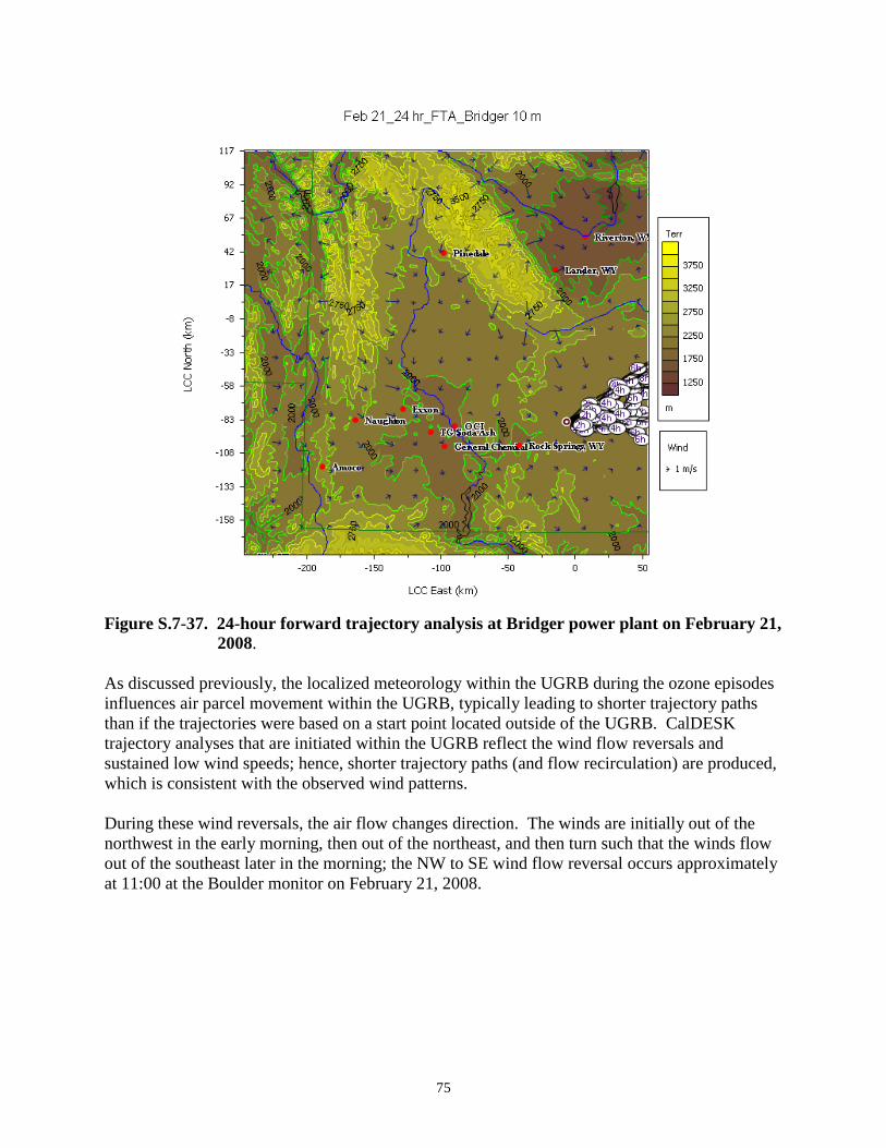
75
Figure S.7-37. 24-hour forward trajectory analysis at Bridger power plant on February 21,
2008.
As discussed previously, the localized meteorology within the UGRB during the ozone episodes
influences air parcel movement within the UGRB, typically leading to shorter trajectory paths
than if the trajectories were based on a start point located outside of the UGRB. CalDESK
trajectory analyses that are initiated within the UGRB reflect the wind flow reversals and
sustained low wind speeds; hence, shorter trajectory paths (and flow recirculation) are produced,
which is consistent with the observed wind patterns.
During these wind reversals, the air flow changes direction. The winds are initially out of the
northwest in the early morning, then out of the northeast, and then turn such that the winds flow
out of the southeast later in the morning; the NW to SE wind flow reversal occurs approximately
at 11:00 at the Boulder monitor on February 21, 2008.

76
CalDESK Forward Trajectory Analyses for February 22, 2008 are shown in Figures S.7-38
through S.7-42.
Figure S.7-38. 24-hour forward trajectory analysis at LaBarge, Wyoming on February 22,
2008
The high pressure ridge continued to weaken during February 22, 2008, while a shortwave low
pressure trough approached southwestern Wyoming from the northwest. Skies became mostly
cloudy during the morning hours and light precipitation spread over the area later in the
afternoon. However, the low level inversion stayed intact well into the afternoon, and ozone
concentrations remained high during most of the day. No IOP operations were conducted this
day because it was anticipated that the stable layer would be mixed-out by the trough by early
morning and, therefore, trapped emission would be dispersed. Instead, the late arrival of the
trough allowed one more day of high ozone concentrations.
As shown in Figure S.7-38, the trajectory analysis for the LaBarge area shows that most of the
possible forward trajectory paths are now moving away from the UGRB during February 22nd
.
Figures S.7-38 through S.7-40 show air parcels tend to be blocked and channeled westward and
then northward around the Wyoming Range, with limited air parcel movement into the UGRB.
There are 1-2 trajectory paths showing air parcel movement from the Moxa Arch and Naughton
areas into the UGRB, however, the vast majority of the air parcel trajectories do not enter the
UGRB, due to the significant terrain blocking and channeling effects of the terrain that make up
the Wyoming Range and the Wasatch Range. Terrain blocking and channeling effects can also
be seen in Figure S.7-42 in the forward trajectories originating from the OCI Trona plant.

77
Figure S.7-39. 24-hour forward trajectory analysis in the Moxa Arch area on February 22,
2008.
Figure S.7-39 shows air parcels tend to be blocked and channeled westward and then northward
around the Wyoming Range, with limited air parcel movement into the UGRB. There are 1-2
trajectory paths showing air parcel movement from the Moxa Arch into the UGRB, however, the
vast majority of the air parcel trajectories do not enter the UGRB, due to the significant terrain
blocking and channeling effects of the terrain that make up the Wyoming Range and the Wasatch
Range.

78
Figure S.7-40. 24-hour forward trajectory analysis at Naughton power plant on February
22, 2008.
There are two forward trajectory paths (2 am and 6 am) which show possible air parcel transport
from the Naughton power plant into the UGRB. A 12-hour back trajectory analysis was
performed at the Boulder monitor location (2 am – 2 pm) for February 22, 2008 to evaluate
potential air parcel trajectories that could reach the Boulder monitor during this same time period
(2 am and 6 am). The results of this back trajectory analysis are shown in Figure S.7-41.
Figure S.7-41 shows the calculated back trajectories of air parcels at the Boulder monitor tend to
originate from within the UGRB, with very little air parcel movement occurring outside of the
UGRB; the air parcels tend to stay within the UGRB during this 12 hour period (2 am – 2 pm)
largely due to localized meteorological conditions in the UGRB. The back trajectory analysis in
Figure S.7-41 shows a limited potential for sources outside the recommended nonattainment area
to affect ozone measured at the Boulder monitor.

79
Figure S.7-41. 12-hour back trajectory analysis at Boulder monitor on February 22, 2008.

80
Figure S.7-42. 24-hour forward trajectory analysis at OCI Trona plant on February 22,
2008.
The predominant paths shown in the trajectory analysis shown in Figure S.7-42 trend to the south
with northerly component to several of the modeled trajectories. Most of the possible forward
trajectory paths are now moving away from the UGRB. Air parcels tend to be blocked and
channeled westward and then northward around the Wyoming Range, with limited air parcel
movement into the UGRB. There is one trajectory path showing air parcel movement from the
OCI toward the UGRB. This trajectory generally parallels the southern boundary of the
proposed nonattainment area along Pacific Creek. While some of the trajectory path may lie
within the proposed nonattainment area, the path does not indicate that sources at OCI cause or
contribute to elevated ozone levels within the proposed nonattainment area.

81
Figure S.7-43. 24-hour forward trajectory analysis at Bridger power plant on February 22,
2008.
The trajectory analysis in Figure S.7-43 shows all modeled trajectories from Bridger not entering
the proposed nonattainment area.
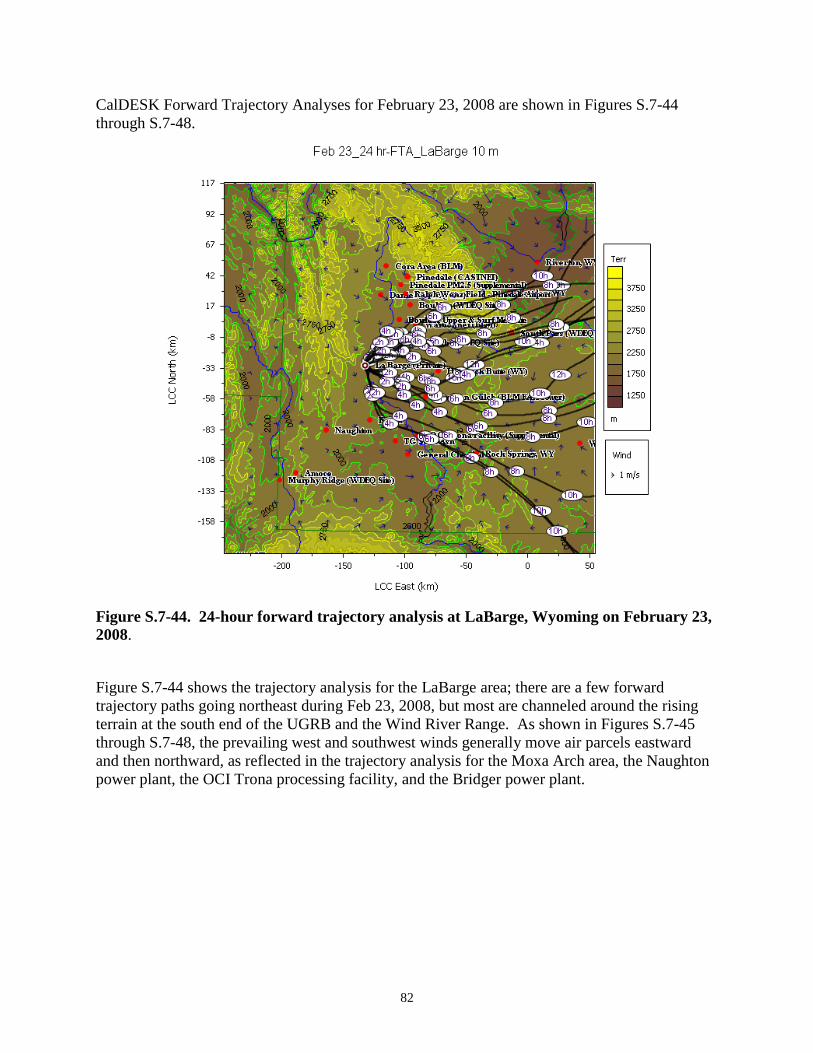
82
CalDESK Forward Trajectory Analyses for February 23, 2008 are shown in Figures S.7-44
through S.7-48.
Figure S.7-44. 24-hour forward trajectory analysis at LaBarge, Wyoming on February 23,
2008.
Figure S.7-44 shows the trajectory analysis for the LaBarge area; there are a few forward
trajectory paths going northeast during Feb 23, 2008, but most are channeled around the rising
terrain at the south end of the UGRB and the Wind River Range. As shown in Figures S.7-45
through S.7-48, the prevailing west and southwest winds generally move air parcels eastward
and then northward, as reflected in the trajectory analysis for the Moxa Arch area, the Naughton
power plant, the OCI Trona processing facility, and the Bridger power plant.
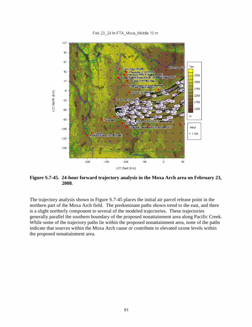
83
Figure S.7-45. 24-hour forward trajectory analysis in the Moxa Arch area on February 23,
2008.
The trajectory analysis shown in Figure S.7-45 places the initial air parcel release point in the
northern part of the Moxa Arch field. The predominant paths shown trend to the east, and there
is a slight northerly component to several of the modeled trajectories. These trajectories
generally parallel the southern boundary of the proposed nonattainment area along Pacific Creek.
While some of the trajectory paths lie within the proposed nonattainment area, none of the paths
indicate that sources within the Moxa Arch cause or contribute to elevated ozone levels within
the proposed nonattainment area.

84
Figure S.7-46. 24-hour forward trajectory analysis at Naughton power plant on February
23, 2008.
The trajectory analysis in Figure S.7-46 shows all modeled trajectories from Naughton not
entering the proposed nonattainment area.
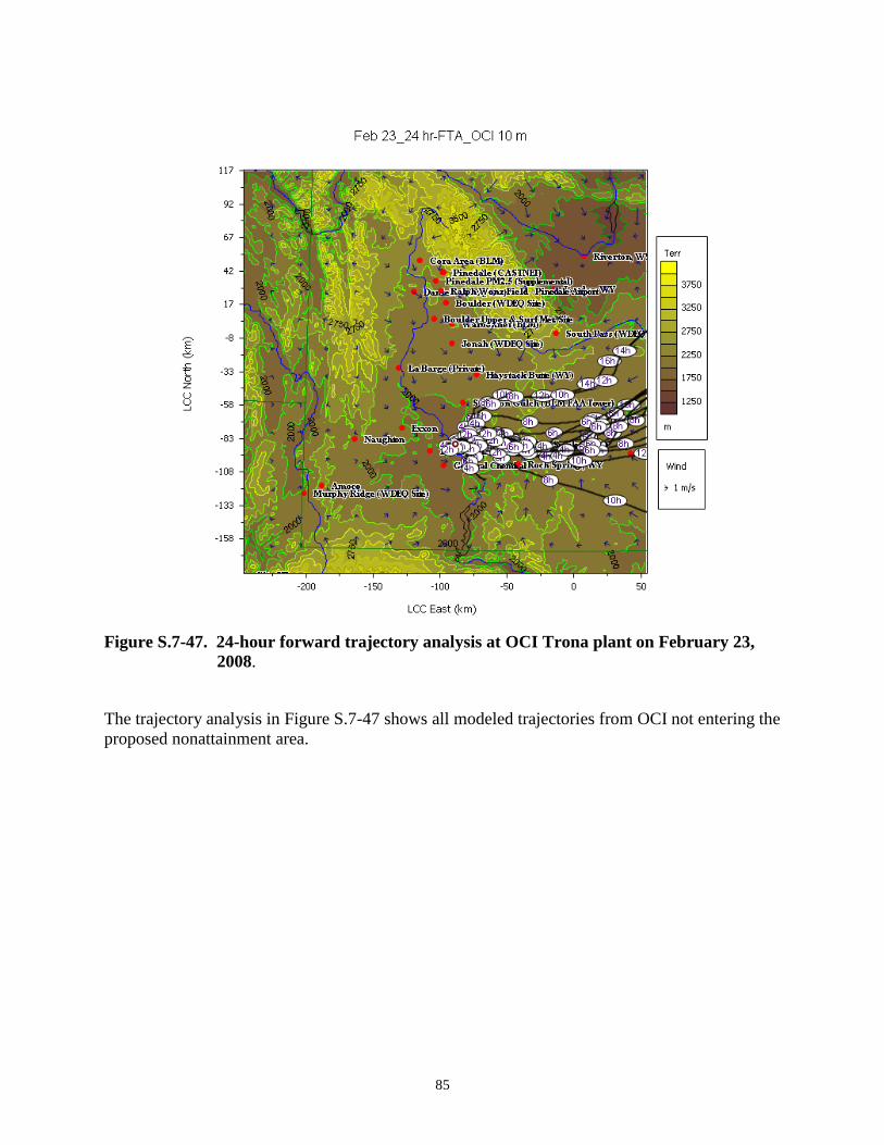
85
Figure S.7-47. 24-hour forward trajectory analysis at OCI Trona plant on February 23,
2008.
The trajectory analysis in Figure S.7-47 shows all modeled trajectories from OCI not entering the
proposed nonattainment area.

86
Figure S.7-48. 24-hour forward trajectory analysis at Bridger power plant on February 23,
2008.
The trajectory analysis in Figure S.7-48 shows all modeled trajectories from Bridger not entering
the proposed nonattainment area.
Summary of Trajectory Analyses
The CalDESK trajectory analyses, based on a three dimensional wind field which incorporates
the localized meteorological data collected during the 2008 field study have allowed AQD to
evaluate air parcel movement as a means of evaluating precursor emissions and ozone transport
into and out of the UGRB. These trajectories indicate that the southern boundary of the
recommended nonattainment area defines an appropriate demarcation where emission sources
within the nonattainment area may contribute ozone or ozone precursors to the Boulder monitor.
Although the Fontenelle Creek, Little Sandy and Pacific drainages are not major topographic
features, these drainage areas influence air movement into the UGRB from locations south of the
recommended nonattainment area during the February 19-23, 2008 ozone episode and define a
reasonable southern boundary for the nonattainment area. AQD has concluded that most, if not
all, of the impact on the Boulder monitor just prior to and during these elevated ozone episodes is
from emission sources located in the nonattainment area as described in this recommendation.

87
SECTION 8
JURISDICTIONAL BOUNDARIES
SYNOPSIS
The Sublette County jurisdictional boundary forms the northern and most of the western and
eastern boundaries of the recommended nonattainment area. The remainder of the boundary is
not jurisdictional but is based on topographical and meteorological considerations.
There is no existing local authority that transcends county boundaries, so the recommended
nonattainment area has no single local administrative authority.
ANALYSIS
The Boulder monitor is located in Sublette County. Sublette County is governed by a three-
person Commission. There are three incorporated towns in Sublette County: Pinedale, Big
Piney and Marbleton. Approximately 80% of the land in Sublette County is owned by the
government: BLM-40%; USFS-36%; State of Wyoming-4%. Federal and state land ownership
in the surrounding counties follows a similar pattern.
The evaluation of the nonattainment area began with the Sublette County jurisdictional area as
the presumptive boundary. This is consistent with EPA guidance in the December 4, 2008
memorandum which states: “Where a violating monitor is not located in a CBSA” (Core Based
Statistical Area) “or CSA,” (Combined Statistical Area) “we recommend that the boundary of the
county containing the monitor serve as the presumptive boundary for the nonattainment area.”
The Boulder monitor is not in a CBSA or CSA.
The recommended nonattainment area includes all of Sublette County; the portion of Lincoln
County northeast of the waterways of Aspen, Fontenelle, and Roney Creeks and northeast of
Fontenelle Reservior and the Green River; and the portion of Sweetwater County northwest of
the waterways of the Green River, the Big Sandy River, Little Sandy Creek, Pacific Creek, and
Whitehorse Creek (see the detailed description in the introduction). This area includes the town
of LaBarge in Lincoln County. The southern boundary of the recommended nonattainment area
is defined based on topographical and meteorological considerations rather than jurisdictional
boundaries. The Sublette County borders to the north, east, and west follow topographic features
(mountain ranges) and are appropriate boundaries for the nonattainment area.
The six counties in Southwest Wyoming which were also included in the analysis are: Teton,
Lincoln, Uinta, Sweetwater, and Fremont. Two Indian Tribal Nations are also located in the
area, the Northern Arapahoe and Eastern Shoshone, at the Wind River Reservation in Fremont
County. The reservation and the counties are shown in Figure S.1-1.
The recommended nonattainment area boundary does not fall under single authority, other than
the State of Wyoming.

88
SECTION 9
LEVEL OF CONTROL OF EMISSION SOURCES
SYNOPSIS
Wyoming’s NSR Program ensures that Best Available Control Technology (BACT) is utilized to
reduce and eliminate air pollution emissions. Wyoming is fairly unique in that BACT is applied
statewide to all new sources, both major sources and minor sources. Since 1995 all oil and gas
production units that were constructed on or after May of 1974 require permits and BACT is
utilized. In two of the gas fields in the proposed nonattainment area, more restrictive emission
control requirements are already in effect. Wyoming has been focused on controlling emissions
from oil and gas sources and has one of the most innovative and effective control programs in
the nation.
While offset programs are traditionally limited to major source applications, the AQD issued an
interim policy in August 2008 requiring offsets of ozone precursor emissions whenever a permit
is issued for a new or modified source in Sublette County, regardless of major source
applicability. This policy results in a net decrease in emissions of ozone precursors with every
permit that is issued. This policy took effect after the ozone exceedances were recorded in the
winter of 2008.
Data is not available for 2009, so it is too early to say with certainty whether this policy has
contributed to reduced ozone concentrations at the Boulder monitor.
ANALYSIS
New Source Review Program
Wyoming’s New Source Review (NSR) Program is a statewide permit program for the
construction of new sources and modification of existing sources as established by Wyoming Air
Quality Standards and Regulations (WAQSR) Chapter 6, Section 2, Permit requirements for
construction, modification and operation and Chapter 6, Section 4, Prevention of significant
deterioration. The primary purpose of the NSR Program is to assure compliance with ambient
standards set to protect public health, assure that Best Available Control Technology is utilized
to reduce and eliminate air pollution emissions, and to prevent deterioration of clean air areas.
Any amount of air contaminant emissions from a facility subjects it to Wyoming’s NSR
Program.
Best Available Control Technology
Due to a desire to maintain and improve Wyoming’s air quality, the Best Available Control
Technology process is applied statewide to new sources, both major sources and minor sources,
under the Wyoming NSR Program’s permitting process. The BACT process is most
appropriately defined as the elimination of pollutants from being emitted into the air whenever
technically and economically feasible to do so. While the Air Quality Division takes the State

89
and federally-required BACT review in the Prevention of Significant Deterioration (PSD)
permitting actions seriously, AQD takes the State-required BACT review in minor source
permitting actions equally as seriously, as the bulk of AQD’s permit applications are for minor
sources.
Control of Oil and Gas Production Sources
Within the recommended nonattainment area, the bulk of the NSR Program activity is due to oil
and gas production and is permitted per the Oil and Gas Production Facilities Chapter 6, Section
2, Permitting Guidance discussed below. The remainder of the activity is attributed to facility
types such as the compressor stations, asphalt plants and crushing and screening operations,
which are permitted per Chapter 6, Section 2 and Chapter 6, Section 4 as described above.
In October 1995, AQD initiated a program to ensure that all oil and gas production units in
southwest Wyoming, as well as the entire state, that were constructed since May of 1974 (the
effective date of Wyoming’s NSR Permit Program) were permitted and that BACT is utilized to
control or eliminate emissions from both major and minor sources. To guide oil and gas
producers through the NSR permitting process, AQD developed an oil and gas industry guidance
document (Guidance) that was released in June of 1997. The Guidance has been revised several
times since it was originally released in June of 1997. The most recent revision took effect in
August of 2007 and includes requirements that apply statewide as well as specifically to the
Jonah and Pinedale Anticline Development (JPAD) Area. The emphasis of the Guidance relies
on a “Presumptive BACT” process, which results in more emissions being controlled earlier in
the life of the production site. This is accomplished by allowing start up or modification of the
production site to occur prior to obtaining a construction permit, provided the operators of such
facilities meet certain emission control requirements, including timely installation of controls,
which have been established through the Presumptive BACT process. Within the JPAD Area,
emission control requirements are more restrictive and become effective upon start up or
modification of the production site.
Under the WAQSR, applicants for permits are required to demonstrate to the Administrator of
the Air Quality Division, that “[t]he proposed facility will not prevent the attainment or
maintenance of any ambient air quality standard.” [WAQSR Chapter 6, Section 2(c)(ii)] To
allow applications for new or modified emission sources of VOC and/or NOx to be processed
while the Division and industry initiatives are taken to reduce the overall emission levels for
VOC and/or NOx in Sublette County, AQD adopted the Interim Policy on Demonstration of
Compliance with WAQSR Chapter 6, Section 2(c)(ii) for Sources in Sublette County on July 21,
2008. The Interim Policy describes options that AQD will consider as an adequate WAQSR
Chapter 6, Section 2(c)(ii) demonstration for permit applications (i.e., new as well as
applications currently under AQD analysis) for new or modified emission sources in Sublette
County.
Options for the Chapter 6, Section 2(c)(ii) demonstration include:
a. Ambient ozone modeling for any application requesting increases in VOCs and/or NOx
emissions.
b. Emission reductions for VOCs and/or NOx emissions.

90
c. Applicants may propose alternate innovative demonstrations to the AQD.
To date, most applicants have chosen to offset VOC and/or NOx emissions and permit
conditions have been established to make the commitments to control emissions federally
enforceable.
During the implementation of the Interim Policy, other long-term approaches (e.g., development
of a regional ozone model and implementation of additional control strategies) to deal with
unacceptable ozone levels in the recommended nonattainment area, will continue to be pursued
by AQD.
Statewide and Industry-wide Control of Volatile Organic Compounds (VOC)
WAQSR Chapter 13 establishes minimum requirements for motor vehicle emission control.
The following federal rules which are incorporated by reference in WAQSR Chapter 5 by
reference contain performance or emission standards for VOCs that may apply to sources within
the recommended nonattainment area and in adjacent areas:
40 CFR Part 60, Subpart D - Standards of Performance for Fossil-Fuel-Fired Steam Generators
for Which Construction is Commenced After August 17, 1971
40 CFR Part 60, Subpart Da - Standards of Performance for Electric Utility Steam Generating
Units for Which Construction is Commenced After September 18, 1978
40 CFR Part 60, Subpart Db - Standards of Performance for Industrial- Commercial-Institutional
Steam Generating Units
40 CFR Part 60, Subpart Dc - Standards of Performance for Small Industrial-Commercial-
Institutional Steam Generating Units
40 CFR Part 60, Subpart I - Standards of Performance for Hot Mix Asphalt Facilities
40 CFR Part 60, Subpart K - Standards of Performance for Storage Vessels for Petroleum
Liquids for Which Construction, Reconstruction, or Modification Commenced After June 11,
1973, and Prior to May 19, 1978
40 CFR Part 60, Subpart Ka - Standards of Performance for Storage Vessels for Petroleum
Liquids for Which Construction, Reconstruction, or Modification Commenced After May 18,
1978, and Prior to July 23, 1984
40 CFR Part 60, Subpart Kb - Standards of Performance for Volatile Organic Liquid Storage
Vessels (Including Petroleum Liquid Storage Vessels) for Which Construction, Reconstruction,
or Modification Commenced After July 23, 1984
40 CFR Part 60, Subpart GG - Standards of Performance for Stationary Gas Turbines

91
40 CFR Part 60, Subpart WWW - Standards of Performance for Municipal Solid Waste Landfills
40 CFR Part 63, Subpart F - National Emission Standards for Organic Hazardous Air Pollutants
From the Synthetic Organic Chemical Manufacturing Industry
40 CFR Part 63, Subpart H - National Emission Standards for Organic Hazardous Air Pollutants
for Equipment Leaks
40 CFR Part 63, Subpart M - National Perchloroethylene Air Emission Standards for Dry
Cleaning Facilities
40 CFR Part 63, Subpart R - National Emission Standards for Gasoline Distribution Facilities
(Bulk Gasoline Terminals and Pipeline Breakout Stations)
40 CFR Part 63, Subpart T - National Emission Standards for Halogenated Solvent Cleaning
40 CFR Part 63, Subpart HH - National Emission Standards for Hazardous Air Pollutants From
Oil and Natural Gas Production Facilities
40 CFR Part 63, Subpart OO - National Emission Standards for Tanks - Level 1
40 CFR Part 63, Subpart PP - National Emission Standards for Containers
40 CFR Part 63, Subpart QQ - National Emission Standards for Surface Impoundments
40 CFR Part 63, Subpart RR - National Emission Standards for Individual Drain Systems
40 CFR Part 63, Subpart SS - National Emission Standards for Closed Vent Systems, Control
Devices, Recovery Devices and Routing to a Fuel Gas System or a Process
40 CFR Part 63, Subpart TT - National Emission Standards for Equipment Leaks - Control Level
1
40 CFR Part 63, Subpart UU - National Emission Standards for Equipment Leaks - Control
Level 2 Standards
40 CFR Part 63, Subpart VV - National Emission Standards for Oil-Water Separators and
Organic-Water Separators
40 CFR Part 63, Subpart WW - National Emission Standards for Storage Vessels (Tanks) -
Control Level 2

92
40 CFR Part 63, Subpart HHH - National Emission Standards for Hazardous Air Pollutants From
Natural Gas Transmission and Storage Facilities
40 CFR Part 63, Subpart UUU - National Emission Standards for Hazardous Air Pollutants for
Petroleum Refineries: Catalytic Cracking Units, Catalytic Reforming Units, and Sulfur
Recovery Units
40 CFR Part 63, Subpart VVV - National Emission Standards for Hazardous Air Pollutants:
Publicly Owned Treatment Works
40 CFR Part 63, Subpart AAAA - National Emission Standards for Hazardous Air Pollutants:
Municipal Solid Waste Landfills
40 CFR Part 63, Subpart EEEE - National Emission Standards for Hazardous Air Pollutants:
Organic Liquids Distribution (Non-Gasoline)
40 CFR Part 63, Subpart YYYY - National Emission Standards for Hazardous Air Pollutants for
Stationary Combustion Turbines
40 CFR Part 63, Subpart ZZZZ - National Emission Standards for Hazardous Air Pollutants for
Stationary Reciprocating Internal Combustion Engines
40 CFR Part 63, Subpart CCCCC - National Emission Standards for Hazardous Air Pollutants
for Coke Ovens: Pushing, Quenching, and Battery Stacks
40 CFR Part 63, Subpart GGGGG - National Emission Standards for Hazardous Air Pollutants:
Site Remediation
40 CFR Part 63, Subpart HHHHH - National Emission Standards for Hazardous Air Pollutants:
Miscellaneous Coating Manufacturing
40 CFR Part 63, Subpart LLLLL - National Emission Standards for Hazardous Air Pollutants:
Asphalt Processing and Asphalt Roofing Manufacturing
Statewide and Industry-wide Nitrogen Oxides (NOx)
WAQSR Chapter 2 establishes ambient air quality standards for those areas under WDEQ’s
jurisdiction. The standard for nitrogen oxides (NOx) is 100 ug/m3 as an annual arithmetic mean.
All facilities that are required to obtain a New Source Review (NSR) permit or a Title V permit
under WAQSR Chapter 6 must demonstrate compliance with the State’s ambient air quality
standard before a permit can be issued.
WAQSR Chapter 3, Section 3 specifies nitrogen dioxide emission standards. Permitting rules
require sources to meet NOx emission standards.
The following federal rules, which are incorporated by reference into Chapter 5, Sections 2 and 3

93
contain performance or emission standards for NOx that may apply to sources in the proposed
nonattainment area and in the surrounding counties:
40 CFR Part 60, Subpart D - Standards of Performance for Fossil-Fuel-Fired Steam Generators
for Which Construction is Commenced After August 17, 1971
40 CFR Part 60, Subpart Da - Standards of Performance for Electric Utility Steam Generating
Units for Which Construction is Commenced After September 18, 1978
40 CFR Part 60, Subpart Db - Standards of performance for Industrial- Commercial-Institutional
Steam Generating Units
40 CFR Part 60, Subpart Dc - Standards of Performance for Small Industrial-Commercial-
Institutional Steam Generating Units
40 CFR Part 60, Subpart GG - Standards of Performance for Stationary Gas Turbines
The following federal New Source Performance Standards have not yet been adopted into State
rules, but are scheduled for adoption. The federal standards will still apply.
NSPS Subpart IIII - Standards of Performance for Stationary Compression Ignition Internal
Combustion Engines
NSPS Subpart JJJJ - Standards of Performance for Stationary Spark Ignition Internal
Combustion Engines
NSPS Subpart KKKK - Standards of Performance for Stationary Combustion Turbines)
Contingency Plans
AQD requested that producers in parts of the proposed nonattainment area prepare emission
reduction plans to be implemented when an ozone advisory is issued. The BLM adopted a
contingency plan requirement in the Pinedale Anticline ROD. Producers, which cumulatively
account for greater than 99% of production in the Pinedale Anticline, submitted contingency
plans to the AQD. During the first quarter of 2009, the AQD issued ozone advisories on
February 4th and 5th. The contingency plans were implemented and no 8-hour ozone values
above 0.075 ppm were recorded at FRM monitors for those days.

94
CONCLUSIONS
The information presented in the preceding nine-factor analysis provides documentation and
compelling evidence supporting a finding that the UGRB, as shown on the map in the
Introduction, should be designated as nonattainment for the 2008 ozone NAAQS. It is important
to note that only areas over which Wyoming has direct air quality jurisdiction are included in this
nonattainment finding and recommendation. The Northern Arapahoe and Eastern Shoshone
Indian Tribes are distinct nations or entities and consequently such Tribal lands (the Wind River
Reservation) are specifically excluded from this designation recommendation.
The Wyoming AQD bases this recommendation on a careful review of the circumstances
surrounding the incidence of elevated ozone events. Elevated ozone in the UGRB is associated
with distinct meteorological conditions. These conditions have occurred in February and March
in some (but not all) of the years since monitoring stations began operation in the UGRB in
2005. Our determination of an appropriate nonattainment area boundary is focused on an
evaluation of EPA’s recommended nine factors, applied to the first quarter of the year, during
which winter ozone episodes occur. This timing does not change how the factors are reviewed,
except for emissions inventory and meteorology. It is important to evaluate inventory and
meteorology during the first quarter of the year in order to focus on the very specific conditions
that lead to high ozone.
The most compelling reasons for the boundary recommendation are based on the meteorological
conditions in place during and just prior to elevated ozone events. Elevated ozone episodes
occurred in 2005, 2006 and 2008; they were associated with very light low-level winds,
sunshine, and snow cover, in conjunction with a strong low-level surface-based temperature or
“capping” inversion. The longest such event, which also resulted in the highest measured ozone
of 122 ppb as an 8-hour average at the Boulder station, has been reviewed in detail and
summarized in Section 7 of this document. Section 7 demonstrates that sources outside the
recommended nonattainment area would not have a significant impact on the Boulder monitor
due to the presence of the inversion and very low winds, which significantly limit emissions and
ozone transport from sources located outside of the UGRB. Using detailed meteorological data
collected during the February 19-23, 2008 ozone episode, a 1 kilometer high resolution (spatial
and temporal) 3-dimensional gridded wind field was developed and used in trajectory analyses.
The trajectory analyses show that air parcels originating at sources located south of the
recommended nonattainment area – including power plants, Trona facilities, and the Moxa Arch
gas field – are generally transported eastward and do not enter the UGRB just prior to and during
the February 19-23, 2008 ozone episode. The meteorological conditions present during this
multi-day ozone episode are representative of the meteorological conditions that were present
during previous wintertime elevated ozone events that occurred in 2005 and 2006. From the
trajectory analyses, it is concluded that emission sources located outside of the recommended
nonattainment boundary could only have a very limited impact on the Boulder monitor, as the
mountains to the west, north and east, along with the observed low wind speeds, would greatly
limit the possibility of emissions transport.

95
The nine-factor analysis also concluded the following:
1. Ozone monitoring outside of the UGRB throughout Wyoming shows attainment of the
2008 NAAQS.
2. Emissions inventories of ozone precursors indicate that sources within the UGRB emit
significant levels of precursors. Emissions from outside of the UGRB (while comparable
to [for VOCs] or greater than [for NOx] emissions from within the UGRB) do not
significantly influence the formation of ozone during and immediately preceding
episodes of elevated ozone.
3. Population densities in Sublette and surrounding counties are very low and are not
expected to be an important factor in ozone formation. This is also true of traffic and
commuting patterns, which would be expected to be more important in urban areas rather
than the rural communities and open spaces of southwest Wyoming.
4. The pace of growth in the oil and gas industry is significantly higher in the UGRB than in
surrounding areas, which would correspond to a more rapid increase in emissions within
the recommended nonattainment area in recent years.
5. Significant terrain features influence the meteorology throughout southwest Wyoming.
Under a stagnating high pressure system, strong temperature inversions and low mixing
heights tend to produce limited atmospheric mixing and precursor emissions can build up
to high concentrations.
The elevated ozone episodes within the UGRB represent a unique situation which is quite
different from other ozone nonattainment areas. The UGRB is rural with a very low population
density; the only significant industry present is oil and gas. The significant terrain features
surrounding the UGRB and the very low wind speeds associated with elevated ozone episodes
may limit the ability of trajectory models, such as the HYSPLIT model, to accurately represent
movement of air parcels within, into and out of the UGRB during these winter ozone events.
Due to the importance of meteorology to the formation of elevated ozone at the Boulder monitor
– that is, ozone at levels that result in an exceedance of the NAAQS occurs during periods
characterized by low mixing heights, temperature inversions and sustained low wind speeds –
any emission reduction applied to sources outside of the UGRB will not result in any meaningful
change in ozone levels at the Boulder monitor during these episodic conditions.
The information presented in this technical support document provides a strong weight-of-
evidence basis for the recommended nonattainment boundary.

Appendix S.1.
Final Report 2008 Upper Green River Winter Ozone Study


Appendix S.3
Population Density by Census Tract

Appendix S.4.A.
2007 Vehicle Miles on State Highways By County

Appendix S.4.B.
Commuting Patterns in Sublette County

Appendix.
Glossary