stata graphics may 2015cc - office of population research · a visual guide to stata graphics,...
TRANSCRIPT

Stata Graphics
Dawn Koffman
Office of Population Research
Princeton University
May 2015
2
Pros:
Many graph types and plot types provided
Multiple plot types may be overlaid
Can easily change overall look of graphs
Same options available for most types of graphs
Very flexible
Cons:
Large syntax: 665 page graphics manual!
Rather slow
Interactive, point-and-click Graph Editor
- However, can record edits and apply them to other graphs
Stata Graphics References:
http://data.princeton.edu/stata/Graphics.html, by German Rodriguez
A Visual Guide To Stata Graphics, Third Edition, by Michael Mitchell
Stata Graphics Manual (may want to start with “graph intro”)
Stata Graphics
3
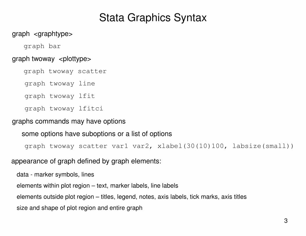
Stata Graphics Syntax
graph <graphtype>
graph bar
graph twoway <plottype>
graph twoway scatter
graph twoway line
graph twoway lfit
graph twoway lfitci
graphs commands may have options
some options have suboptions or a list of options
graph twoway scatter var1 var2, xlabel(30(10)100, labsize(small))
appearance of graph defined by graph elements:
data - marker symbols, lines
elements within plot region – text, marker labels, line labels
elements outside plot region – titles, legend, notes, axis labels, tick marks, axis titles
size and shape of plot region and entire graph

4
sysuse uslifeexp.dta, clear
graph twoway line le year
/* OR */
twoway line le year
/* OR */
line le year
40
50
60
70
80
life e
xpecta
ncy
1900 1920 1940 1960 1980 2000Year
Stata Graphics Syntax: A Simple Example
5
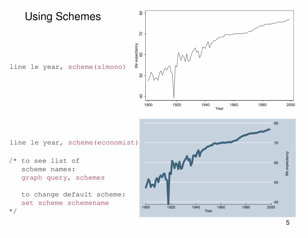
line le year, scheme(s1mono)
line le year, scheme(economist)
/* to see list of
scheme names:
graph query, schemes
to change default scheme:
set scheme schemename
*/
40
50
60
70
80
life e
xpecta
ncy
1900 1920 1940 1960 1980 2000Year
40
50
60
70
80
life e
xpecta
ncy
1900 1920 1940 1960 1980 2000Year
Using Schemes

6
line le_wmale le_wfemale le_bmale le_bfemale year
30
40
50
60
70
80
1900 1920 1940 1960 1980 2000Year
Life expectancy, white males Life expectancy, white females
Life expectancy, black males Life expectancy, black females
Multiple Dependent Variables

7
Adding Text
line le_wmale le_wfemale le_bmale le_bfemale year ///
, text(32 1920 “{bf:1918} {it:Influenza} Pandemic", place(3))
1918 Influenza Pandemic
30
40
50
60
70
80
1900 1920 1940 1960 1980 2000Year
Life expectancy, white males Life expectancy, white females
Life expectancy, black males Life expectancy, black females

8
scatter ///
le year if year >= 1950 ///
|| lfit le year if year >= 1950
/* OR */
twoway ///
(scatter le year if year >= 1950) ///
(lfit le year if year >= 1950)
/* OR */
#delimit ;
twoway
(scatter le year if year >= 1950)
(lfit le year if year >= 1950);
#delimit cr
scatter le year if year >= 1950 || lfit le year if year >= 1950
/* OR */
Overlaying Two-Way Plot Types
68
70
72
74
76
1950 1960 1970 1980 1990 2000Year
life expectancy Fitted values

9
scatter le year if year >= 1925 ///
|| lfit le year if year >= 1925 & ///
year < 1950 ///
|| lfit le year if year >= 1950
/* OR */
twoway ///
(scatter le year if year >= 1925) ///
(lfit le year if year >= 1925 & ///
year < 1950) ///
(lfit le year if year >= 1950)
/* OR */
#delimit ;
scatter le year if year >= 1925
|| lfit le year if year >= 1925 & year < 1950
|| lfit le year if year >= 1950;
#delimit cr
55
60
65
70
75
1920 1940 1960 1980 2000Year
life expectancy Fitted values
Fitted values
Overlaying Two-Way Plot Types

10
#delimit ;
scatter le_male le_female year if year >= 1950
|| lfit le_male year if year >= 1950
|| lfit le_female year if year >= 1950;
#delimit cr
65
70
75
80
1950 1960 1970 1980 1990 2000Year
Life expectancy, males Life expectancy, females
Fitted values Fitted values
Overlaying Two-Way Plot Types
11
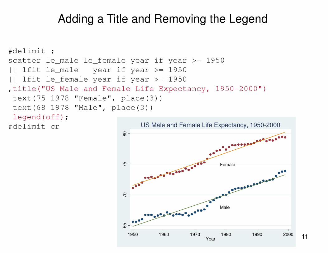
Adding a Title and Removing the Legend
#delimit ;
scatter le_male le_female year if year >= 1950
|| lfit le_male year if year >= 1950
|| lfit le_female year if year >= 1950
,title("US Male and Female Life Expectancy, 1950-2000")
text(75 1978 "Female", place(3))
text(68 1978 "Male", place(3))
legend(off);
#delimit cr
Female
Male
65
70
75
80
1950 1960 1970 1980 1990 2000Year
US Male and Female Life Expectancy, 1950-2000
12
50
60
70
80
Life e
xp
ecta
ncy a
t bir
th
20 40 60 80 100Percent of population with access to safe water
Linear fit 95% CI
Life expectancy at birth by access to safe water, 1998
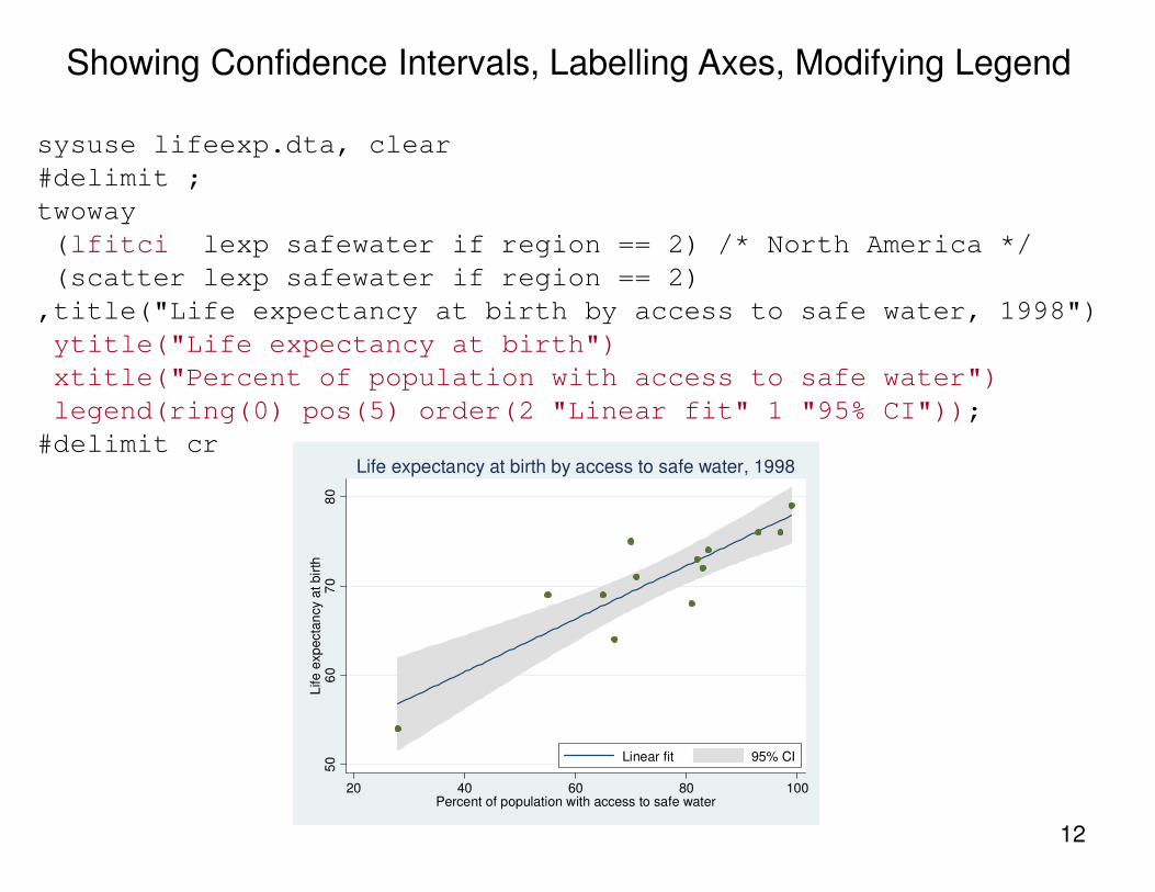
sysuse lifeexp.dta, clear
#delimit ;
twoway
(lfitci lexp safewater if region == 2) /* North America */
(scatter lexp safewater if region == 2)
,title("Life expectancy at birth by access to safe water, 1998")
ytitle("Life expectancy at birth")
xtitle("Percent of population with access to safe water")
legend(ring(0) pos(5) order(2 "Linear fit" 1 "95% CI"));
#delimit cr
Showing Confidence Intervals, Labelling Axes, Modifying Legend
13
Canada
Cuba
Dominican Republic
El Salvador
Guatemala
Haiti
Honduras
Jamaica
Mexico
Nicaragua
Panama
Puerto Rico
Trinidad and Tobago
50
60
70
80
Life e
xp
ecta
ncy a
t bir
th
20 40 60 80 100Percent of population with access to safe water
Linear fit 95% CI
North America
Life expectancy at birth by access to safe water, 1998
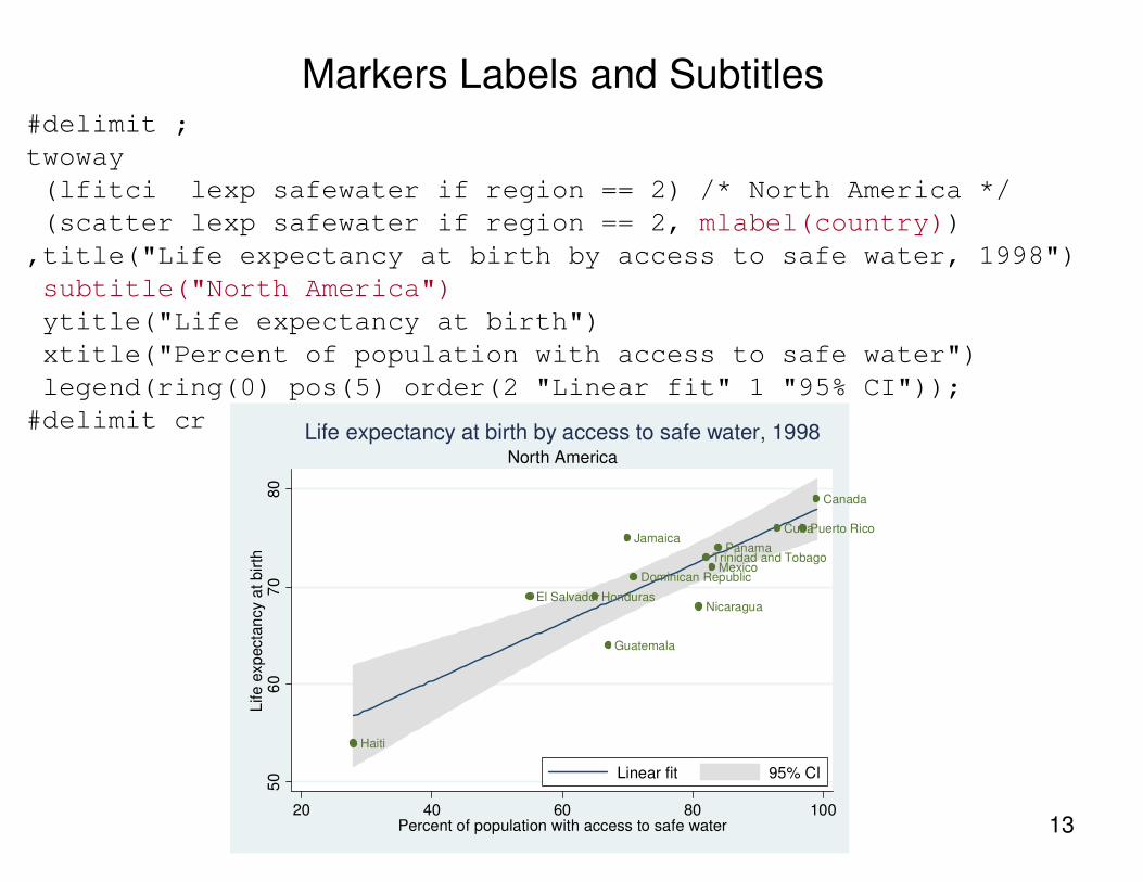
#delimit ;
twoway
(lfitci lexp safewater if region == 2) /* North America */
(scatter lexp safewater if region == 2, mlabel(country))
,title("Life expectancy at birth by access to safe water, 1998")
subtitle("North America")
ytitle("Life expectancy at birth")
xtitle("Percent of population with access to safe water")
legend(ring(0) pos(5) order(2 "Linear fit" 1 "95% CI"));
#delimit cr
Markers Labels and Subtitles

14
Canada
Cuba
Dominican Republic
El Salvador
Guatemala
Haiti
Honduras
Jamaica
Mexico
Nicaragua
PanamaPuerto Rico
Trinidad and Tobago
50
60
70
80
Life e
xp
ecta
ncy a
t bir
th
20 40 60 80 100Percent of population with access to safe water
Linear fit 95% CI
North America
Life expectancy at birth by access to safe water, 1998
generate pos = 12 if country == "Panama"
replace pos = 12 if country == "Honduras"
replace pos = 10 if country == "Cuba"
replace pos = 9 if country == "Jamaica"
replace pos = 9 if country == "El Salvador"
replace pos = 9 if country == "Trinidad and Tobago"
replace pos = 9 if country == "Dominican Republic"
#delimit ;
twoway
(lfitci lexp safewater if region == 2) /* North America */
(scatter lexp safewater if region == 2
, mlabel(country) mlabvposition(pos))
,title("Life expectancy at birth by access to safe water, 1998")
subtitle("North America")
ytitle("Life expectancy at birth")
xtitle("Percent of population with access to safe water")
legend(ring(0) pos(5) order(2 "Linear fit" 1 "95% CI"))
plotregion(margin(r+10));
#delimit cr
Position of Marker Labels

15
Canada
Cuba
Dominican Republic
El Salvador
Guatemala
Haiti
Honduras
Jamaica
Mexico
Nicaragua
Panama
Puerto Rico
Trinidad and TobagoArgentina
Bolivia
Brazil
Chile
ColombiaEcuadorParaguayPeru
UruguayVenezuela
55
60
65
70
75
80
Life e
xp
ecta
ncy a
t bir
th
20 40 60 80 100Percent of population with access to safe water
North and South America
Life expectancy at birth by access to safe water, 1998
#delimit ;
twoway
(scatter lexp safewater if region == 2 | region == 3
,mlabel(country))
,title("Life expectancy at birth by access to safe water, 1998")
subtitle("North and South America")
ytitle("Life expectancy at birth")
xtitle("Percent of population with access to safe water")
plotregion(margin(r+10));
#delimit cr
Position of Marker Labels
16
Canada
Cuba
Dominican Republic
El Salvador
Guatemala
Haiti
Honduras
Jamaica
Mexico
Nicaragua
Panama
Puerto Rico
Trinidad and TobagoArgentina
Bolivia
Brazil
Chile
ColombiaEcuadorParaguayPeru
UruguayVenezuela
55
60
65
70
75
80
Life e
xp
ecta
ncy a
t bir
th
20 40 60 80 100Percent of population with access to safe water
North America
South America
North and South America
Life expectancy at birth by access to safe water, 1998
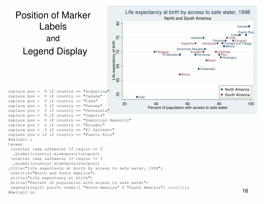
replace pos = 9 if country == "Argentina"
replace pos = 9 if country == "Canada"
replace pos = 9 if country == "Cuba"
replace pos = 9 if country == "Panama"
replace pos = 9 if country == "Venezuela"
replace pos = 9 if country == "Jamaica"
replace pos = 9 if country == "Dominican Republic"
replace pos = 9 if country == "Ecuador"
replace pos = 9 if country == "El Salvador"
replace pos = 12 if country == "Puerto Rico"
#delimit ;
twoway
(scatter lexp safewater if region == 2
,mlabel(country) mlabvposition(pos))
(scatter lexp safewater if region == 3
,mlabel(country) mlabvposition(pos))
,title("Life expectancy at birth by access to safe water, 1998")
subtitle("North and South America")
ytitle("Life expectancy at birth")
xtitle("Percent of population with access to safe water")
legend(ring(0) pos(5) order(1 "North America" 2 "South America") cols(1));
#delimit cr
Position of Marker
Labels
and
Legend Display
17
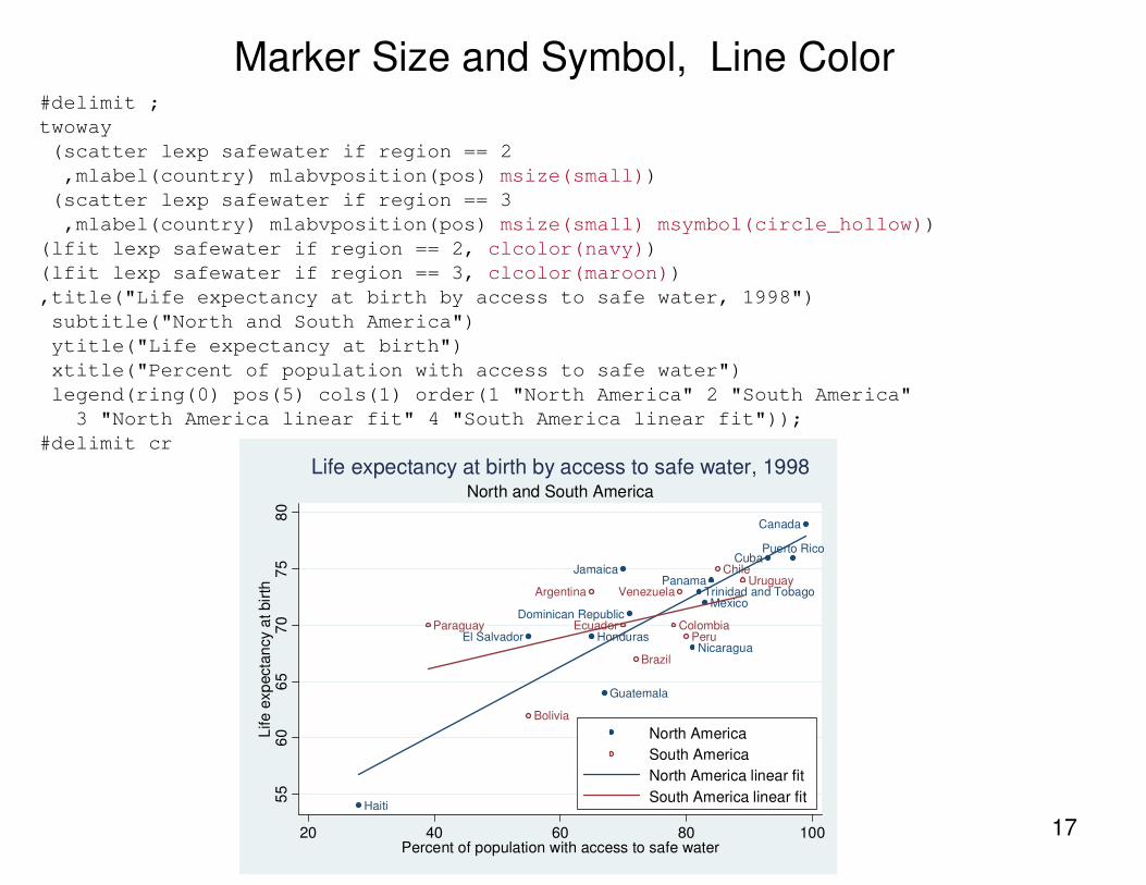
Marker Size and Symbol, Line Color
Canada
Cuba
Dominican Republic
El Salvador
Guatemala
Haiti
Honduras
Jamaica
Mexico
Nicaragua
Panama
Puerto Rico
Trinidad and TobagoArgentina
Bolivia
Brazil
Chile
ColombiaEcuadorParaguayPeru
UruguayVenezuela
55
60
65
70
75
80
Life e
xp
ecta
ncy a
t bir
th
20 40 60 80 100Percent of population with access to safe water
North America
South America
North America linear fit
South America linear fit
North and South America
Life expectancy at birth by access to safe water, 1998
#delimit ;
twoway
(scatter lexp safewater if region == 2
,mlabel(country) mlabvposition(pos) msize(small))
(scatter lexp safewater if region == 3
,mlabel(country) mlabvposition(pos) msize(small) msymbol(circle_hollow))
(lfit lexp safewater if region == 2, clcolor(navy))
(lfit lexp safewater if region == 3, clcolor(maroon))
,title("Life expectancy at birth by access to safe water, 1998")
subtitle("North and South America")
ytitle("Life expectancy at birth")
xtitle("Percent of population with access to safe water")
legend(ring(0) pos(5) cols(1) order(1 "North America" 2 "South America"
3 "North America linear fit" 4 "South America linear fit"));
#delimit cr

18
Canada
Cuba
Dominican Republic
El Salvador
Guatemala
Haiti
Honduras
Jamaica
Mexico
Nicaragua
Panama
Puerto Rico
Trinidad and TobagoArgentina
Bolivia
Brazil
Chile
ColombiaEcuadorParaguayPeru
UruguayVenezuela
55
60
65
70
75
80
Life e
xp
ecta
ncy a
t bir
th
20 40 60 80 100Percent of population with access to safe water
North America
South America
North America linear fit
South America linear fit
North and South America
Life expectancy at birth by access to safe water, 1998
#delimit ;
twoway
(scatter lexp safewater if region == 2
,mlabel(country) mlabvposition(pos) msize(small) mcolor(black) mlabcolor(black))
(scatter lexp safewater if region == 3
,mlabel(country) mlabvposition(pos) msize(small) mcolor(black) mlabcolor(black)
msymbol(circle_hollow))
(lfit lexp safewater if region == 2, clcolor(black))
(lfit lexp safewater if region == 3, clcolor(black) clpattern(dash))
,title("Life expectancy at birth by access to safe water, 1998", color(black))
subtitle("North and South America")
ytitle("Life expectancy at birth")
xtitle("Percent of population with access to safe water")
legend(ring(0) pos(5) cols(1) order(1 "North America" 2 "South America"
3 "North America linear fit" 4 "South America linear fit"));
#delimit cr
Marker and Marker Label Color, Line Style
19
50
60
70
80
50
60
70
80
20 40 60 80 100 20 40 60 80 100
Eur & C.Asia N.A.
S.A. Total
Life
exp
ecta
ncy a
t b
irth
Percent of population with access to safe waterGraphs by Region
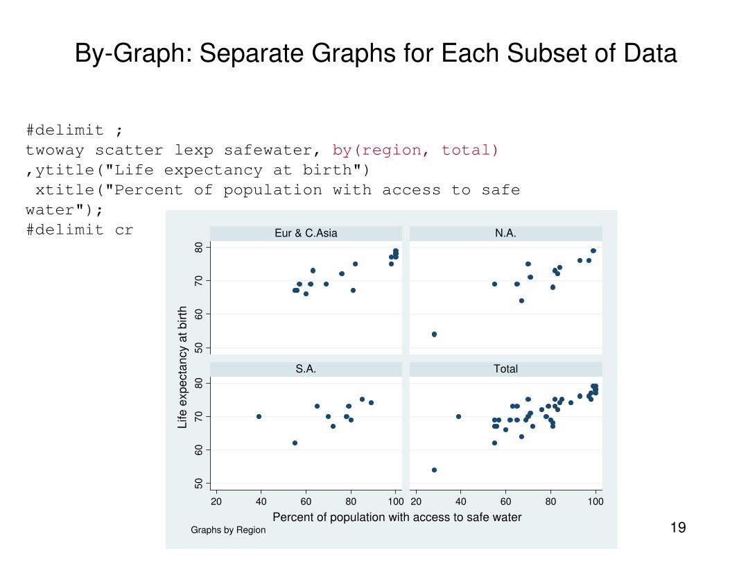
#delimit ;
twoway scatter lexp safewater, by(region, total)
,ytitle("Life expectancy at birth")
xtitle("Percent of population with access to safe
water");
#delimit cr
By-Graph: Separate Graphs for Each Subset of Data
20
50
60
70
80
50
60
70
80
20 40 60 80 10020 40 60 80 100
Eur & C.Asia N.A.
S.A. Total
Life
exp
ecta
ncy a
t b
irth
Percent of population with access to safe water
Life expectancy by access to safe water
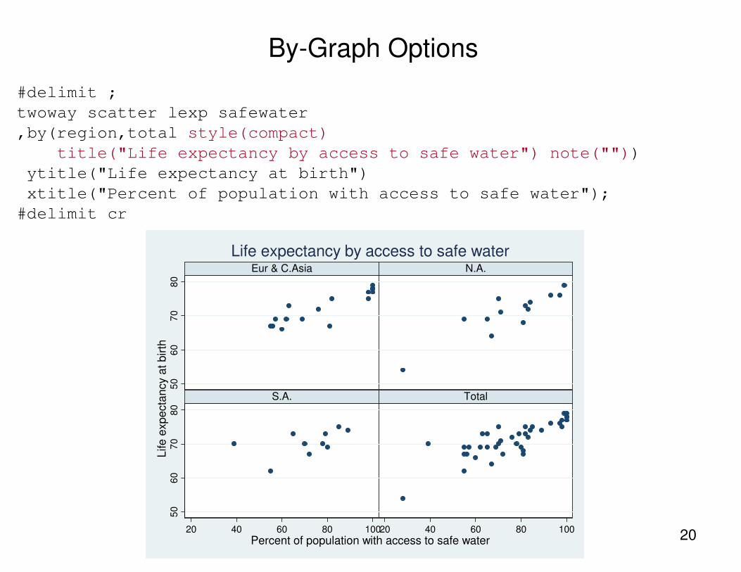
#delimit ;
twoway scatter lexp safewater
,by(region,total style(compact)
title("Life expectancy by access to safe water") note(""))
ytitle("Life expectancy at birth")
xtitle("Percent of population with access to safe water");
#delimit cr
By-Graph Options
21
55
60
65
70
75
80
55
60
65
70
75
80
30 40 50 60 70 80 90 100 30 40 50 60 70 80 90 100
Eur & C.Asia N.A.
S.A. Total
Life
exp
ecta
ncy a
t b
irth
Percent of population with access to safe water
Life expectancy by access to safe water
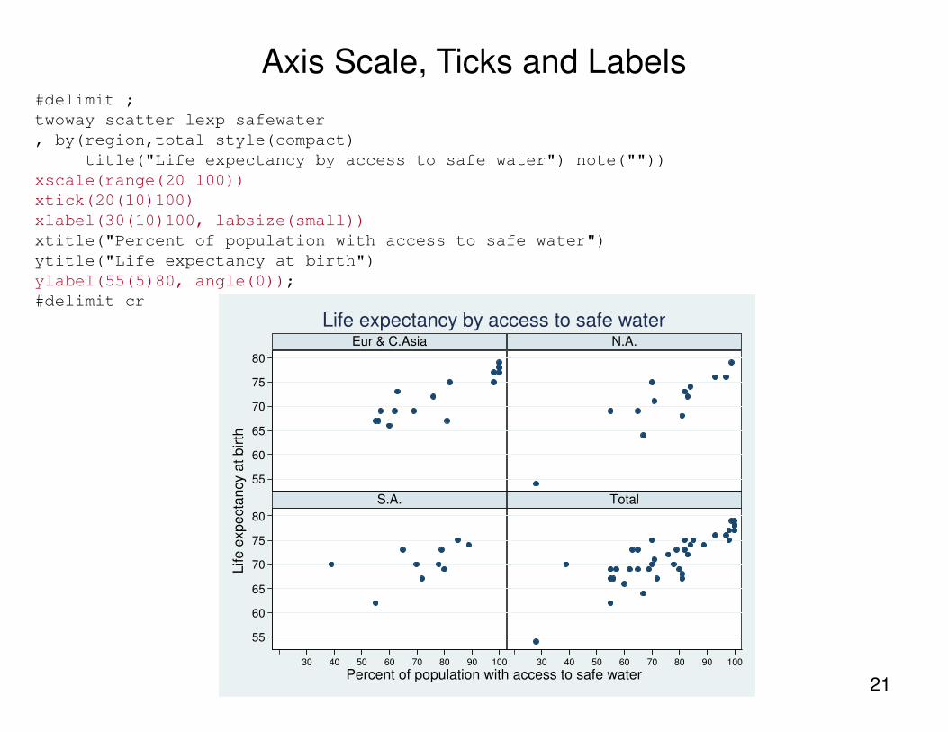
#delimit ;
twoway scatter lexp safewater
, by(region,total style(compact)
title("Life expectancy by access to safe water") note(""))
xscale(range(20 100))
xtick(20(10)100)
xlabel(30(10)100, labsize(small))
xtitle("Percent of population with access to safe water")
ytitle("Life expectancy at birth")
ylabel(55(5)80, angle(0));
#delimit cr
Axis Scale, Ticks and Labels
22
Canada
Cuba
Dominican Republic
El Salvador
Guatemala
Haiti
Honduras
Jamaica
Mexico
Nicaragua
Panama
Puerto Rico
Trinidad and Tobago
55
60
65
70
75
80
Life e
xp
ecta
ncy a
t bir
th
20 40 60 80 100Percent of population with access to safe water
North America
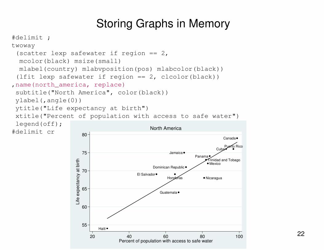
#delimit ;
twoway
(scatter lexp safewater if region == 2,
mcolor(black) msize(small)
mlabel(country) mlabvposition(pos) mlabcolor(black))
(lfit lexp safewater if region == 2, clcolor(black))
,name(north_america, replace)
subtitle("North America", color(black))
ylabel(,angle(0))
ytitle("Life expectancy at birth")
xtitle("Percent of population with access to safe water")
legend(off);
#delimit cr
Storing Graphs in Memory

23
Argentina
Bolivia
Brazil
Chile
ColombiaEcuadorParaguay
Peru
Uruguay
Venezuela
60
65
70
75
Life e
xp
ecta
ncy a
t bir
th
40 50 60 70 80 90Percent of population with access to safe water
South America
#delimit ;
twoway
(scatter lexp_sa safewater if region == 3,
mcolor(black) msize(small)
mlabel(country) mlabvposition(pos) mlabcolor(black))
(lfit lexp safewater if region == 3, clcolor(black))
,name(south_america, replace)
subtitle("South America", color(black))
ylabel(, angle(0))
ytitle("Life expectancy at birth")
xtitle("Percent of population with access to safe water")
legend(off);
#delimit cr
Storing Graphs in Memory
24
Canada
Cuba
Dominican RepublicEl Salvador
Guatemala
Haiti
Honduras
Jamaica
Mexico
Nicaragua
Panama
Puerto Rico
Trinidad and Tobago
55
60
65
70
75
80
Life e
xpecta
ncy a
t bir
th
20 40 60 80 100Percent of population with access to safe water
North America
Argentina
Bolivia
Brazil
Chile
ColombiaEcuadorParaguayPeru
UruguayVenezuela
60
65
70
75
Life e
xpecta
ncy a
t bir
th
40 50 60 70 80 90Percent of population with access to safe water
South America
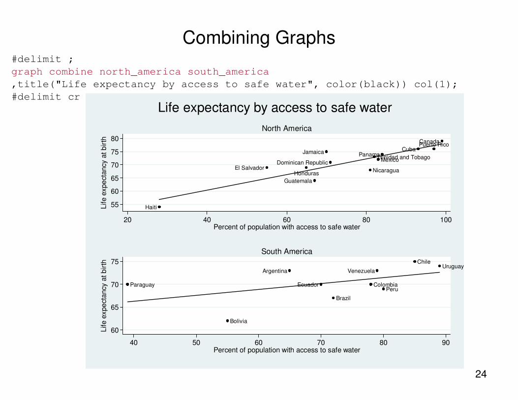
Life expectancy by access to safe water
#delimit ;
graph combine north_america south_america
,title("Life expectancy by access to safe water", color(black)) col(1);
#delimit cr
Combining Graphs

25
Canada
Cuba
Dominican Republic
El Salvador
Guatemala
Haiti
Honduras
Jamaica
Mexico
Nicaragua
Panama
Puerto Rico
Trinidad and Tobago
55
60
65
70
75
80
Life e
xpecta
ncy a
t birth
20 40 60 80 100Percent of population with access to safe water
North America
Argentina
Bolivia
Brazil
Chile
ColombiaEcuadorParaguayPeru
UruguayVenezuela
55
60
65
70
75
80
Life e
xpecta
ncy a
t birth
20 40 60 80 100Percent of population with access to safe water
South America
Life expectancy by access to safe water
#delimit ;
graph combine north_america south_america
,title
("Life expectancy by access to safe water",
color(black))
xcommon ycommon
xsize(7) ysize(10.5)
col(1);
#delimit cr
Combining
Graphs

26
save graph in portable format (format determined by filename extension)
vector formats contain drawing instructions (.wmf .emf .ps .eps .pdf)
resolution independent
work well if graph my be resized
graph export north_america.wmf
raster formats save graph pixel-by-pixel (.png)
use current resolution
work well if including graph on web pages
graph export north_america.png
Saving Stata Graphs

clear
input str14 country tvhome birth5years idealnum age1stbirth school agemarriage
bangladesh 33.9 .6 2.3 17.7 4.5 15.2
bolivia 74.8 .8 2.6 20.3 7.6 20.1
colombia 93.4 .4 2.4 20.7 8.6 20.3
dr 83 .5 3.2 19.9 8.6 18.3
egypt 95.9 .7 2.9 21.3 7.3 19.7
haiti 27.9 .8 3.2 20.7 4.3 19.4
india 47.9 .6 2.4 19.2 4.3 17.1
indonesia 74 .5 2.8 20.7 7.5 19.3
morocco 66.6 .7 3.3 21.4 2.7 19.6
nepal 50.7 .6 2.2 19.6 3.6 17.4
pakistan 57.8 .9 4.1 20.5 2.8 18.4
peru 78.1 .6 2.5 21.1 8.8 20.6
end
label variable tvhome "TV at home (%)"
label variable school "years of school"
label variable birth5years "births in last 5 years"
label variable idealnum "ideal number of children"
label variable age1stbirth "age at first birth"
label variable school "years of school"
label variable agemarriage "age at first marriage“
Country Level Data
27
Data source: Westoff, Charles F., et. al. In preparation. Leading Indicators of Changes in Fertility in Sub-Saharan Africa.
Demographic and Health Surveys, DHS Analytical Studies. ICF International, Calverton, MD, USA.
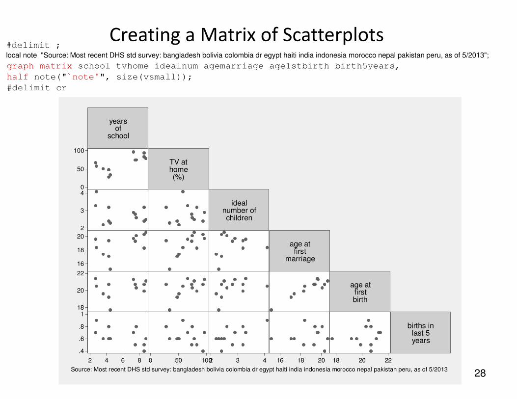
graph matrix school tvhome idealnum agemarriage age1stbirth birth5years,
half note("`note'", size(vsmall));
#delimit cr
yearsof
school
TV athome(%)
idealnumber ofchildren
age atfirst
marriage
age atfirstbirth
births inlast 5years
2 4 6 8
0
50
100
0 50 100
2
3
4
2 3 4
16
18
20
16 18 20
18
20
22
18 20 22
.4
.6
.8
1
Source: Most recent DHS std survey: bangladesh bolivia colombia dr egypt haiti india indonesia morocco nepal pakistan peru, as of 5/2013
Creating a Matrix of Scatterplots
28
#delimit ;
local note "Source: Most recent DHS std survey: bangladesh bolivia colombia dr egypt haiti india indonesia morocco nepal pakistan peru, as of 5/2013";
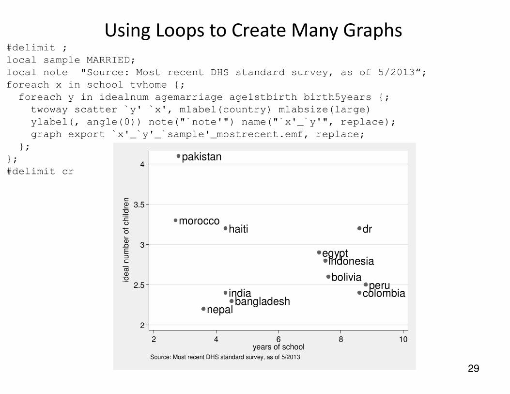
#delimit ;
local sample MARRIED;
local note "Source: Most recent DHS standard survey, as of 5/2013“;
foreach x in school tvhome {;
foreach y in idealnum agemarriage age1stbirth birth5years {;
twoway scatter `y' `x', mlabel(country) mlabsize(large)
ylabel(, angle(0)) note("`note'") name("`x'_`y'", replace);
graph export `x'_`y'_`sample'_mostrecent.emf, replace;
};
};
#delimit cr
bangladesh
bolivia
colombia
dr
egypt
haiti
india
indonesia
morocco
nepal
pakistan
peru
2
2.5
3
3.5
4
ide
al n
um
be
r o
f ch
ildre
n
2 4 6 8 10years of school
Source: Most recent DHS standard survey, as of 5/2013
Using Loops to Create Many Graphs
29
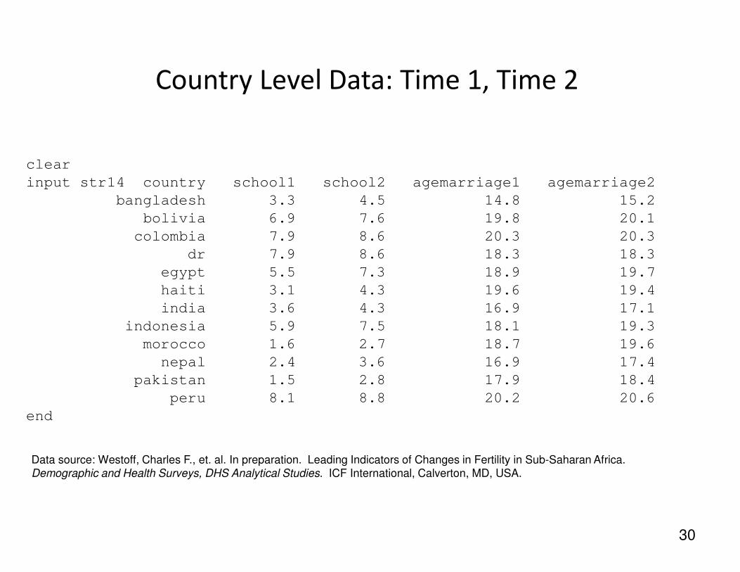
clear
input str14 country school1 school2 agemarriage1 agemarriage2
bangladesh 3.3 4.5 14.8 15.2
bolivia 6.9 7.6 19.8 20.1
colombia 7.9 8.6 20.3 20.3
dr 7.9 8.6 18.3 18.3
egypt 5.5 7.3 18.9 19.7
haiti 3.1 4.3 19.6 19.4
india 3.6 4.3 16.9 17.1
indonesia 5.9 7.5 18.1 19.3
morocco 1.6 2.7 18.7 19.6
nepal 2.4 3.6 16.9 17.4
pakistan 1.5 2.8 17.9 18.4
peru 8.1 8.8 20.2 20.6
end
Country Level Data: Time 1, Time 2
30
Data source: Westoff, Charles F., et. al. In preparation. Leading Indicators of Changes in Fertility in Sub-Saharan Africa.
Demographic and Health Surveys, DHS Analytical Studies. ICF International, Calverton, MD, USA.
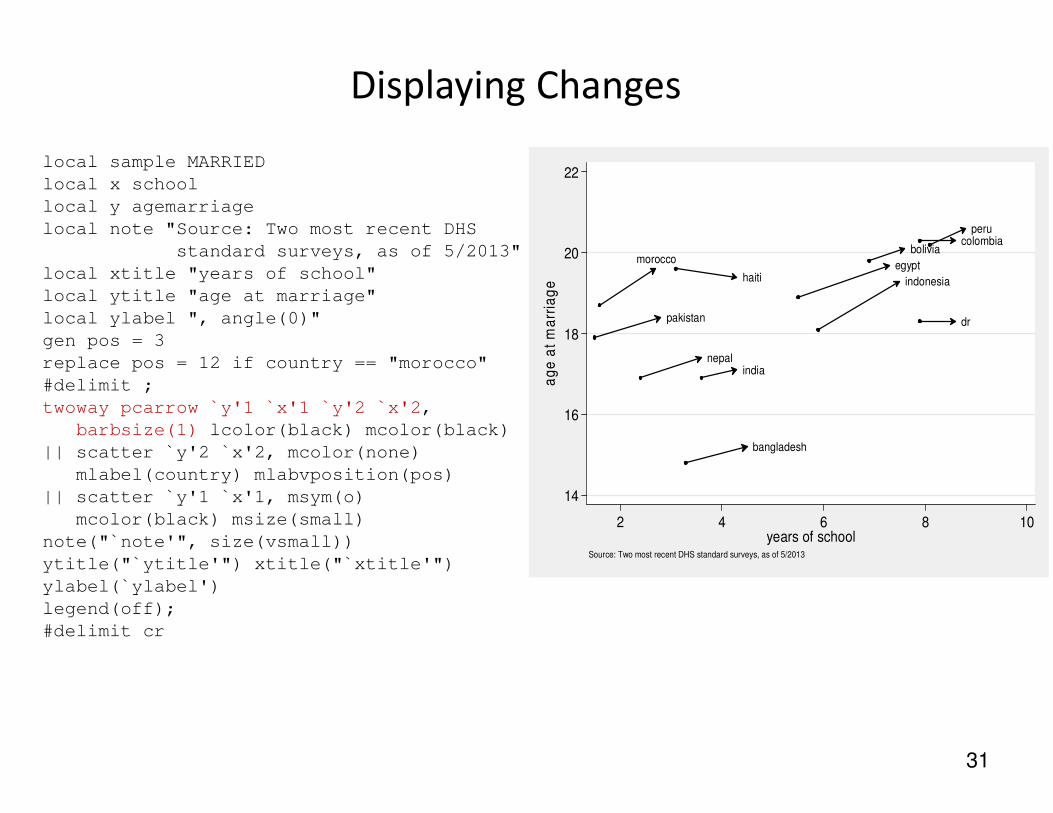
local sample MARRIED
local x school
local y agemarriage
local note "Source: Two most recent DHS
standard surveys, as of 5/2013"
local xtitle "years of school"
local ytitle "age at marriage"
local ylabel ", angle(0)"
gen pos = 3
replace pos = 12 if country == "morocco"
#delimit ;
twoway pcarrow `y'1 `x'1 `y'2 `x'2,
barbsize(1) lcolor(black) mcolor(black)
|| scatter `y'2 `x'2, mcolor(none)
mlabel(country) mlabvposition(pos)
|| scatter `y'1 `x'1, msym(o)
mcolor(black) msize(small)
note("`note'", size(vsmall))
ytitle("`ytitle'") xtitle("`xtitle'")
ylabel(`ylabel')
legend(off);
#delimit cr
Displaying Changes
bangladesh
boliviacolombia
dr
egypthaiti
india
indonesia
morocco
nepal
pakistan
peru
14
16
18
20
22
ag
e a
t m
arr
iag
e
2 4 6 8 10years of school
Source: Two most recent DHS standard surveys, as of 5/2013
31

0
2
4
6
8
Pe
rce
nt
0 5 10 15 20hourly wage
Source: Stata 12 NLSW 1988 extract
Hourly Wage Distribution, Women 40-44
Histogram
32
set scheme s2mono
sysuse nlsw88.dta, clear
keep if age >=40 | age <= 44
#delimit ;
twoway histogram wage if wage <= 20, percent fcolor(gs12) lcolor(gs12) bin(30)
title("Hourly Wage Distribution, Women 40-44")
note("Source: Stata 12 NLSW 1988 extract", span)
ylabel(, angle(0));
#delimit cr

0
2
4
6
8
10
Pe
rce
nt
0 5 10 15 20hourly wage
Union
Non-Union
Source: Stata 12 NLSW 1988 extract
Hourly Wage Distribution by Union Status, Women 40-44
#delimit ;
twoway histogram wage if union == 1 & wage <= 20,
percent fcolor(gs12) lcolor(gs12) bin(30) ||
histogram wage if union == 0 & wage <= 20,
percent fcolor(none) lcolor(black) bin(30)
title("Hourly Wage Distribution by Union Status, Women 40-44")
note("Source: Stata 12 NLSW 1988 extract", span) ylabel(, angle(0))
legend(ring(0) pos(1) cols(1) order(1 "Union" 2 "Non-Union"));
#delimit cr
Overlaying Histograms
33

0
10
20
30
40
ho
url
y w
ag
e
white black otherSource: Stata 12 NLSW 1988 extract
Hourly Wage by Race, Women 40-44 (n=918)
#delimit ;
graph box wage if age >= 40 & age <= 44, over(race)
title("Hourly Wage by Race, Women 40-44 (n=918)")
note("Source: Stata 12 NLSW 1988 extract")
ylabel(, angle(0));
#delimit cr
Boxplot
34
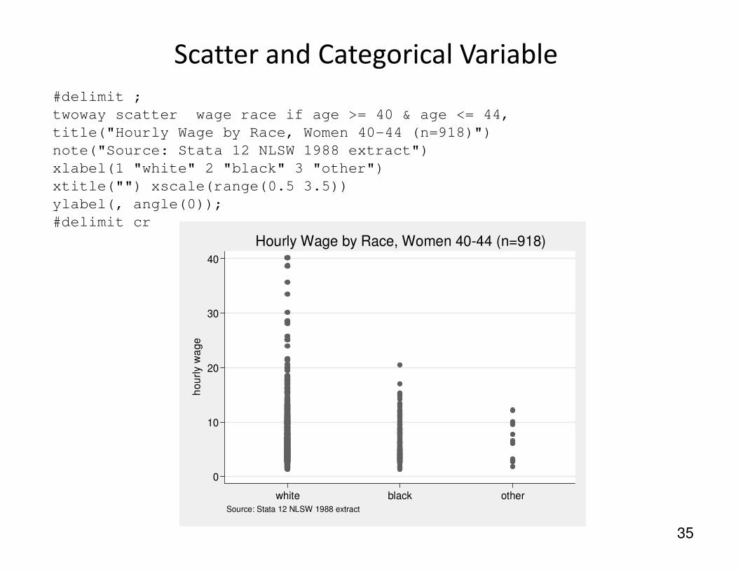
#delimit ;
twoway scatter wage race if age >= 40 & age <= 44,
title("Hourly Wage by Race, Women 40-44 (n=918)")
note("Source: Stata 12 NLSW 1988 extract")
xlabel(1 "white" 2 "black" 3 "other")
xtitle("") xscale(range(0.5 3.5))
ylabel(, angle(0));
#delimit cr
0
10
20
30
40
ho
url
y w
ag
e
white black otherSource: Stata 12 NLSW 1988 extract
Hourly Wage by Race, Women 40-44 (n=918)
Scatter and Categorical Variable
35

0
10
20
30
40
ho
url
y w
ag
e
white black otherSource: Stata 12 NLSW 1988 extract
Hourly Wage by Race, Women 40-44 (n=918)
#delimit ;
twoway scatter wage race if age >= 40 & age <= 44,
jitter(25) msize(tiny) mcolor(gs5)
title("Hourly Wage by Race, Women 40-44 (n=918)")
note("Source: Stata 12 NLSW 1988 extract")
xlabel(1 "white" 2 "black" 3 "other", noticks)
xtitle("") xscale(range(0.5 3.5)) ylabel(, angle(0));
#delimit cr
Scatter with Jitter and Categorical Variable
36

egen median = median(wage), by(race)
egen upq = pctile(wage), p(75) by(race)
egen loq = pctile(wage), p(25) by(race)
egen iqr = iqr(wage), by(race)
#delimit ;
twoway rbar med upq race, barwidth(0.7) blc(black) bfc(none) lwidth(medthick) ||
rbar med loq race, barwidth(0.7) blc(black) bfc(none) lwidth(medthick)
title("Hourly Wage by Race, Women 40-44 (n=918)")
note("Source: Stata 12 NLSW 1988 extract")
xlabel(1 "white" 2 "black" 3 "other", noticks) xtitle("")
xscale(range(0.5 3.5))
yscale(range(0 42))
ylabel(0 (10) 40, angle(0))
ytitle("hourly wage")
legend(off);
#delimit cr
Using twoway rbar
37
0
10
20
30
40
ho
url
y w
ag
e
white black otherSource: Stata 12 NLSW 1988 extract
Hourly Wage by Race, Women 40-44 (n=918)

egen median = median(wage), by(race)
egen upq = pctile(wage), p(75) by(race)
egen loq = pctile(wage), p(25) by(race)
egen iqr = iqr(wage), by(race)
#delimit ;
twoway scatter wage race, jitter(25) msize(tiny) mcolor(gs9) ||
rbar med upq race, barwidth(0.70) blc(black) bfc(none) lwidth(medthick)||
rbar med loq race, barwidth(0.70) blc(black) bfc(none) lwidth(medthick)
title("Hourly Wage by Race, Women 40-44 (n=918)")
note("Source: Stata 12 NLSW 1988 extract")
xlabel(1 "white" 2 "black" 3 "other", noticks) xtitle("")
xscale(range(0.5 3.5))
yscale(range(0 42))
ylabel(0 (10) 40, angle(0))
ytitle("hourly wage")
legend(off);
#delimit cr
Boxplot with Scatter
38
0
10
20
30
40h
ou
rly w
ag
e
white black otherSource: Stata 12 NLSW 1988 extract
Hourly Wage by Race, Women 40-44 (n=918)
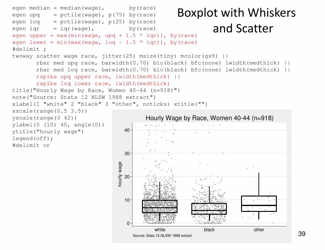
egen median = median(wage), by(race)
egen upq = pctile(wage), p(75) by(race)
egen loq = pctile(wage), p(25) by(race)
egen iqr = iqr(wage), by(race)
egen upper = max(min(wage, upq + 1.5 * iqr)), by(race)
egen lower = min(max(wage, loq - 1.5 * iqr)), by(race)
#delimit ;
twoway scatter wage race, jitter(25) msize(tiny) mcolor(gs9) ||
rbar med upq race, barwidth(0.70) blc(black) bfc(none) lwidth(medthick) ||
rbar med loq race, barwidth(0.70) blc(black) bfc(none) lwidth(medthick) ||
rspike upq upper race, lwidth(medthick) ||
rspike loq lower race, lwidth(medthick)
title("Hourly Wage by Race, Women 40-44 (n=918)")
note("Source: Stata 12 NLSW 1988 extract")
xlabel(1 "white" 2 "black" 3 "other", noticks) xtitle("")
xscale(range(0.5 3.5))
yscale(range(0 42))
ylabel(0 (10) 40, angle(0))
ytitle("hourly wage")
legend(off);
#delimit cr
Boxplot with Whiskers
and Scatter
39
0
10
20
30
40
ho
url
y w
ag
e
white black otherSource: Stata 12 NLSW 1988 extract
Hourly Wage by Race, Women 40-44 (n=918)
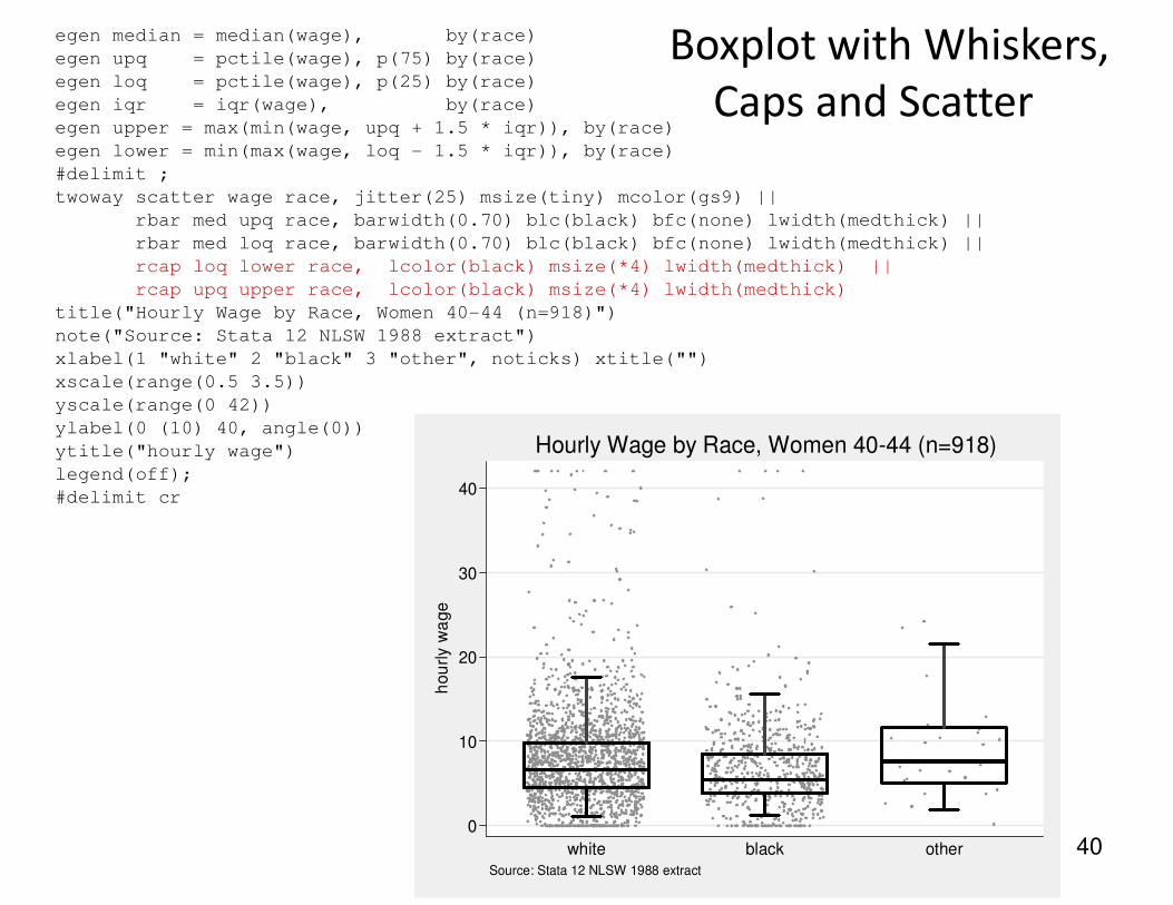
egen median = median(wage), by(race)
egen upq = pctile(wage), p(75) by(race)
egen loq = pctile(wage), p(25) by(race)
egen iqr = iqr(wage), by(race)
egen upper = max(min(wage, upq + 1.5 * iqr)), by(race)
egen lower = min(max(wage, loq - 1.5 * iqr)), by(race)
#delimit ;
twoway scatter wage race, jitter(25) msize(tiny) mcolor(gs9) ||
rbar med upq race, barwidth(0.70) blc(black) bfc(none) lwidth(medthick) ||
rbar med loq race, barwidth(0.70) blc(black) bfc(none) lwidth(medthick) ||
rcap loq lower race, lcolor(black) msize(*4) lwidth(medthick) ||
rcap upq upper race, lcolor(black) msize(*4) lwidth(medthick)
title("Hourly Wage by Race, Women 40-44 (n=918)")
note("Source: Stata 12 NLSW 1988 extract")
xlabel(1 "white" 2 "black" 3 "other", noticks) xtitle("")
xscale(range(0.5 3.5))
yscale(range(0 42))
ylabel(0 (10) 40, angle(0))
ytitle("hourly wage")
legend(off);
#delimit cr
Boxplot with Whiskers,
Caps and Scatter
400
10
20
30
40
ho
url
y w
ag
e
white black otherSource: Stata 12 NLSW 1988 extract
Hourly Wage by Race, Women 40-44 (n=918)
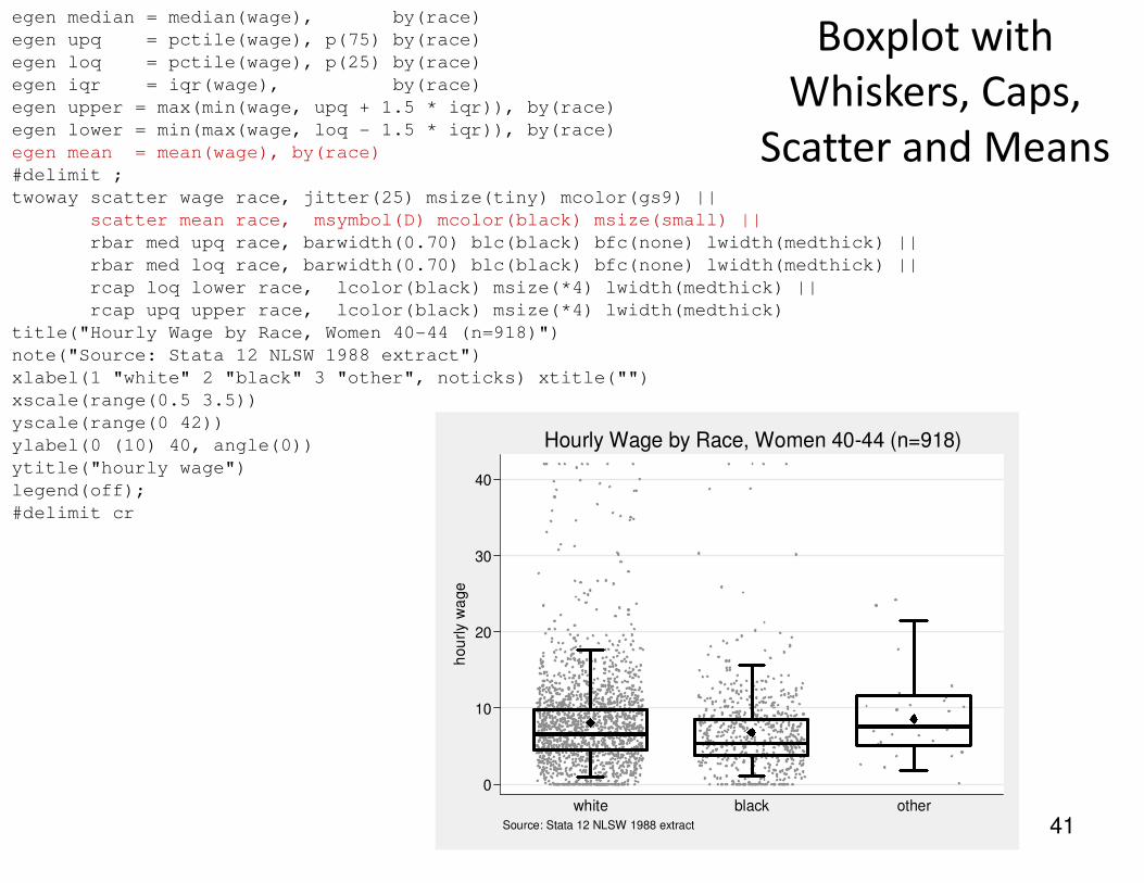
egen median = median(wage), by(race)
egen upq = pctile(wage), p(75) by(race)
egen loq = pctile(wage), p(25) by(race)
egen iqr = iqr(wage), by(race)
egen upper = max(min(wage, upq + 1.5 * iqr)), by(race)
egen lower = min(max(wage, loq - 1.5 * iqr)), by(race)
egen mean = mean(wage), by(race)
#delimit ;
twoway scatter wage race, jitter(25) msize(tiny) mcolor(gs9) ||
scatter mean race, msymbol(D) mcolor(black) msize(small) ||
rbar med upq race, barwidth(0.70) blc(black) bfc(none) lwidth(medthick) ||
rbar med loq race, barwidth(0.70) blc(black) bfc(none) lwidth(medthick) ||
rcap loq lower race, lcolor(black) msize(*4) lwidth(medthick) ||
rcap upq upper race, lcolor(black) msize(*4) lwidth(medthick)
title("Hourly Wage by Race, Women 40-44 (n=918)")
note("Source: Stata 12 NLSW 1988 extract")
xlabel(1 "white" 2 "black" 3 "other", noticks) xtitle("")
xscale(range(0.5 3.5))
yscale(range(0 42))
ylabel(0 (10) 40, angle(0))
ytitle("hourly wage")
legend(off);
#delimit cr
Boxplot with
Whiskers, Caps,
Scatter and Means
41
0
10
20
30
40
ho
url
y w
ag
e
white black other
Source: Stata 12 NLSW 1988 extract
Hourly Wage by Race, Women 40-44 (n=918)
6.41
8.04
6.35
7.66
10.6411.41
9.82 10.00
not college grad college grad
single married single married
Source: Stata 12 NLSW 1988 extract
by union status, marital status, and college graduation
1988 Mean Hourly Wage of Women Age 40-44
nonunion union
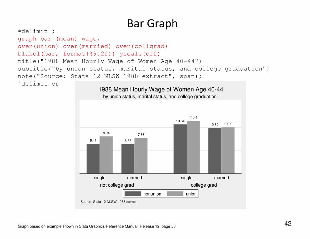
#delimit ;
graph bar (mean) wage,
over(union) over(married) over(collgrad)
blabel(bar, format(%9.2f)) yscale(off)
title("1988 Mean Hourly Wage of Women Age 40-44")
subtitle("by union status, marital status, and college graduation")
note("Source: Stata 12 NLSW 1988 extract", span);
#delimit cr
Bar Graph
42Graph based on example shown in Stata Graphics Reference Manual, Release 12, page 58.

0 5 101520
college grad
not college grad
Construction
Manufacturing
Transport/Comm/Utility
Public Administration
Finance/Ins/Real Estate
Business/Repair Svc
Professional Services
Entertainment/Rec Svc
Wholesale/Retail Trade
Ag/Forestry/Fisheries
Personal Services
Mining
Transport/Comm/Utility
Finance/Ins/Real Estate
Public Administration
Manufacturing
Business/Repair Svc
Construction
Professional Services
Entertainment/Rec Svc
Wholesale/Retail Trade
Ag/Forestry/Fisheries
Personal Services
Source: Stata 12 NLSW 1988 extract
1988 Mean Hourly Wage of Women Age 40-44
#delimit ;
graph hbar wage, over(ind, sort(1))
over(collgrad)
title("1988 Mean Hourly Wage of Women
Age 40-44", span size(med))
note("Source: Stata 12 NLSW 1988
extract", span)
nofill ytitle("") ysize(8);
#delimit cr
Horizontal Bar Graph
Graph based on example shown in Stata Graphics Reference
Manual, Release 12, page 70.

0 5 101520
college grad
not college grad
Construction
Manufacturing
Transport/Comm/Utility
Public Administration
Finance/Ins/Real Estate
Business/Repair Svc
Professional Services
Entertainment/Rec Svc
Wholesale/Retail Trade
Ag/Forestry/Fisheries
Personal Services
Mining
Transport/Comm/Utility
Finance/Ins/Real Estate
Public Administration
Manufacturing
Business/Repair Svc
Construction
Professional Services
Entertainment/Rec Svc
Wholesale/Retail Trade
Ag/Forestry/Fisheries
Personal Services
Source: Stata 12 NLSW 1988 extract
1988 Mean Hourly Wage of Women Age 40-44
#delimit ;
graph dot wage, over(ind, sort(1))
over(collgrad)
title("1988 Mean Hourly Wage of Women
Age 40-44", span size(med))
note("Source: Stata 12 NLSW 1988
extract", span)
nofill ytitle("") ysize(8);
#delimit cr
Dot Plot
0 10 20 30
college grad
not college grad
ConstructionManufacturing
Transport/Comm/Utility
Finance/Ins/Real EstateBusiness/Repair SvcPublic Administration
Entertainment/Rec Svc
Professional ServicesWholesale/Retail Trade
Ag/Forestry/FisheriesPersonal Services
Mining
Transport/Comm/Utility
Finance/Ins/Real EstateEntertainment/Rec Svc
Public Administration
ConstructionBusiness/Repair Svc
ManufacturingProfessional Services
Wholesale/Retail Trade
Ag/Forestry/FisheriesPersonal Services
Source: Stata 12 NLSW 1988 extract
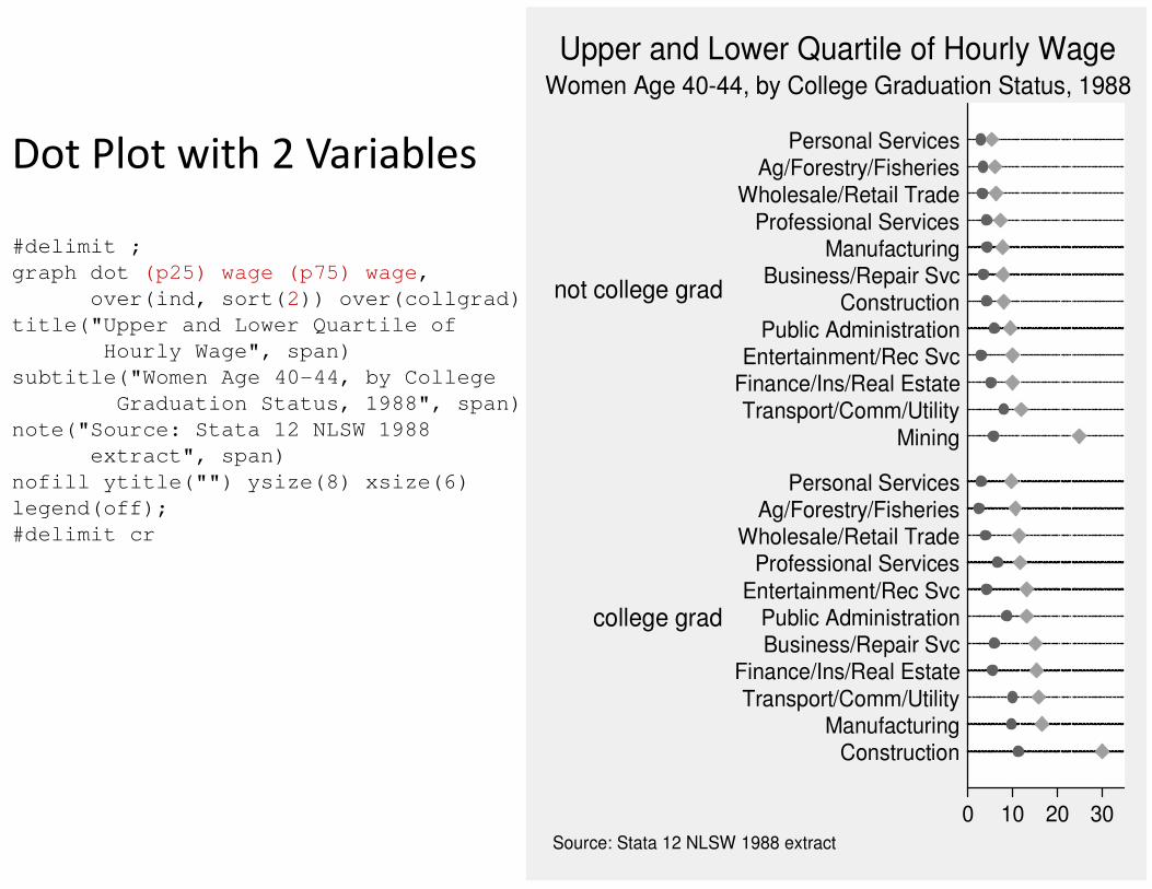
Women Age 40-44, by College Graduation Status, 1988
Upper and Lower Quartile of Hourly Wage
#delimit ;
graph dot (p25) wage (p75) wage,
over(ind, sort(2)) over(collgrad)
title("Upper and Lower Quartile of
Hourly Wage", span)
subtitle("Women Age 40-44, by College
Graduation Status, 1988", span)
note("Source: Stata 12 NLSW 1988
extract", span)
nofill ytitle("") ysize(8) xsize(6)
legend(off);
#delimit cr
Dot Plot with 2 Variables

agegrp maletotal femtotal
1. Under 5 9,810,733 9,365,065
2. 5 to 9 10,523,277 10,026,228
3. 10 to 14 10,520,197 10,007,875
4. 15 to 19 10,391,004 9,828,886
5. 20 to 24 9,687,814 9,276,187
6. 25 to 29 9,798,760 9,582,576
7. 30 to 34 10,321,769 10,188,619
8. 35 to 39 11,318,696 11,387,968
9. 40 to 44 11,129,102 11,312,761
10. 45 to 49 9,889,506 10,202,898
11. 50 to 54 8,607,724 8,977,824
12. 55 to 59 6,508,729 6,960,508
13. 60 to 64 5,136,627 5,668,820
14. 65 to 69 4,400,362 5,133,183
15. 70 to 74 3,902,912 4,954,529
16. 75 to 79 3,044,456 4,371,357
17. 80 to 84 1,834,897 3,110,470
Population Data
46
05
10
15
20
Ag
e c
ate
go
ry
-10,000,000 -5,000,000 0 5,000,000 10,000,000
Male Total Female Total
Source: US Census Bureau, Census 2000, Tables 1, 2 and 3
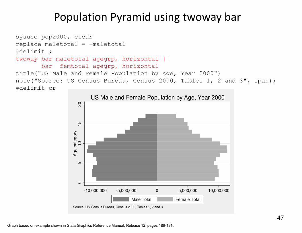
US Male and Female Population by Age, Year 2000
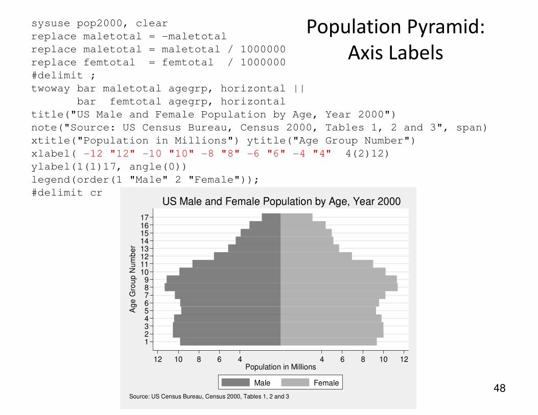
sysuse pop2000, clear
replace maletotal = -maletotal
#delimit ;
twoway bar maletotal agegrp, horizontal ||
bar femtotal agegrp, horizontal
title("US Male and Female Population by Age, Year 2000")
note("Source: US Census Bureau, Census 2000, Tables 1, 2 and 3", span);
#delimit cr
Population Pyramid using twoway bar
47Graph based on example shown in Stata Graphics Reference Manual, Release 12, pages 189-191.
123456789
1011121314151617
Ag
e G
rou
p N
um
be
r
12 10 8 6 4 4 6 8 10 12Population in Millions
Male Female
Source: US Census Bureau, Census 2000, Tables 1, 2 and 3
US Male and Female Population by Age, Year 2000
sysuse pop2000, clear
replace maletotal = -maletotal
replace maletotal = maletotal / 1000000
replace femtotal = femtotal / 1000000
#delimit ;
twoway bar maletotal agegrp, horizontal ||
bar femtotal agegrp, horizontal
title("US Male and Female Population by Age, Year 2000")
note("Source: US Census Bureau, Census 2000, Tables 1, 2 and 3", span)
xtitle("Population in Millions") ytitle("Age Group Number")
xlabel( -12 "12" -10 "10" -8 "8" -6 "6" -4 "4" 4(2)12)
ylabel(1(1)17, angle(0))
legend(order(1 "Male" 2 "Female"));
#delimit cr
Population Pyramid:
Axis Labels
48

Under 5
5 to 9
10 to 14
15 to 19
20 to 24
25 to 29
30 to 34
35 to 39
40 to 44
45 to 49
50 to 54
55 to 59
60 to 64
65 to 69
70 to 74
75 to 79
80 to 84
Male Female
12 10 8 6 4 4 6 8 10 12Population in Millions
Source: US Census Bureau, Census 2000, Tables 1, 2 and 3
US Male and Female Population by Age, Year 2000
sysuse pop2000, clear
replace maletotal = -maletotal
replace maletotal = maletotal / 1000000
replace femtotal = femtotal / 1000000
gen zero = 0
#delimit ;
twoway bar maletotal agegrp, horizontal bfc(gs7) blc(gs7) ||
bar femtotal agegrp, horizontal bfc(gs11) blc(gs11) ||
scatter agegrp zero, mlabel(agegrp) mlabcolor(black) msymbol(none)
title("US Male and Female Population by Age, Year 2000")
note("Source: US Census Bureau, Census 2000, Tables 1, 2 and 3", span)
xtitle("Population in Millions") ytitle("Age Group Number")
ytitle("") yscale(noline) ylabel(none)
xlabel( -12 "12" -10 "10" -8 "8" -6 "6" -4 "4" 4(2)12)
legend(off) text(15 -8 "Male") text(15 8 "Female");
#delimit cr
Population Pyramid:
Age Group Labels
49