stat 425: introduction to bayesian analysismarina/stat425/part3_hm.pdf1 when there is no within...

STAT 425: Introduction to Bayesian Analysis

Marina Vannucci

Rice University, USA

Fall 2017

Marina Vannucci (Rice University, USA) Bayesian Analysis (Part 3) Fall 2017 1 / 36

Part 3: Hierarchical and Linear Models

Hierarchical models

Linear regression models

Generalized linear models (logistic and Poisson)


Hierarchical models - Outline

Hierarchical models

Random effect models

Mixed effect models


Hierarchical models

The exercise of specifying a model over several levels is calledhierarchical modeling, with each new distribution forming a new levelin the hierarchy.

In a hierarchical model, the observations are given distributionsconditional on parameters, and the parameters in turn have distributionsconditional on additional parameters called hyperparameters.Non-hierarchical models are usually inappropriate for hierarchical data

with few parameters, they generally cannot fit the data adequatelywith many parameters, they tend to “overfit” the data.

Hierarchical models allow information to be shared across groups ofobservations.


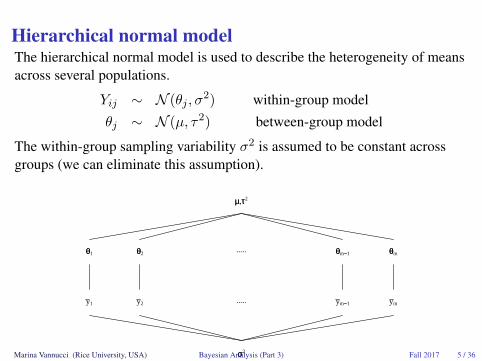
Hierarchical normal modelThe hierarchical normal model is used to describe the heterogeneity of meansacross several populations.

Yij ∼ N (θj , σ2) within-group model

θj ∼ N (µ, τ2) between-group model

The within-group sampling variability σ2 is assumed to be constant acrossgroups (we can eliminate this assumption).

µµ,ττ2

θθ1 θθ2..... θθm−−1 θθm

y1 y2 ..... ym−−1 ym

σσ2Marina Vannucci (Rice University, USA) Bayesian Analysis (Part 3) Fall 2017 5 / 36

The unknown quantities are:

the group-specific means {θ1, . . . , θm}the within-group sampling variability σ2

the mean and variance of the population of group-specific means (µ, τ2)

Posterior inference for these parameters can be made by constructing a Gibbssampler which approximates p(θ1, . . . , θm, σ2, µ, τ2|y1, . . . , ym) byiteratively sampling each parameter from its full conditional distribution.


Example: High school math achievement

Representative sample of U.S. public schools (160 schools)

Within each school, a random sample of students is selected (14 to 67)with a total of 7185 students.

The primary outcome, Yij , is a standardized measure of mathachievement for student i in school j.

Additional covariates are collected on each student.


One-way ANOVA

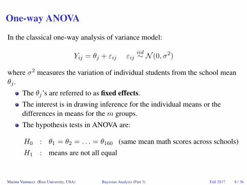
In the classical one-way analysis of variance model:

Yij = θj + εij εijiid∼ N (0, σ2)

where σ2 measures the variation of individual students from the school meanθj .

The θj’s are referred to as fixed effects.

The interest is in drawing inference for the individual means or thedifferences in means for the m groups.

The hypothesis tests in ANOVA are:

H0 : θ1 = θ2 = . . . = θ160 (same mean math scores across schools)

H1 : means are not all equal


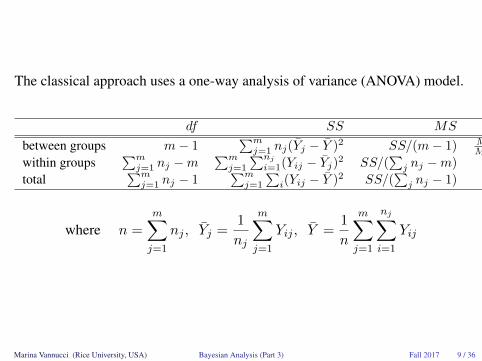
The classical approach uses a one-way analysis of variance (ANOVA) model.

df SS MS F

between groups m− 1∑m

j=1 nj(Yj − Y )2 SS/(m− 1) MSBMSW

within groups∑m

j=1 nj −m∑m

j=1

∑nj

i=1(Yij − Yj)2 SS/(∑

j nj −m)

total∑m

j=1 nj − 1∑m

j=1

∑i(Yij − Y )2 SS/(

∑j nj − 1)

where n =

m∑j=1

nj , Yj =1

nj

m∑j=1

Yij , Y =1

n

m∑j=1

nj∑i=1

Yij


If ratio of between to within mean squares is significantly < 1 (F -testp-value ≤ 0.05), reject H0 and use separate estimates: θj = Yj for eachj.

If the ratio of mean squares is not “statistically significant” (F -testp-value > 0.05), pooling the means is reasonable: θ1 = . . . = θm = Y .

anova(aov(y ˜ school))Analysis of Variance Table

Df Sum Sq Mean Sq F value Pr(>F)school 159 64907 408 10.429 2.2e-16 ***Residuals 7025 274970 39

So we either treat all the means as equal or all different. Two extremes.


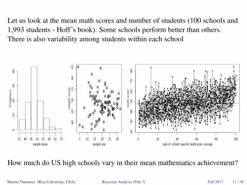
Let us look at the mean math scores and number of students (100 schools and1,993 students - Hoff’s book). Some schools perform better than others.There is also variability among students within each school

sample mean

Fre

qu

en

cy

35 40 45 50 55 60 65 70

01

02

03

04

0

●

●

●

●

●

●

●

● ●

●

●

●●

●

●●

●

●

●

●

●

●

●

●●

●

●

●

●

● ●●

●

●

●

●

●

●

●

●

●

●

●

●

●

●

●

●

●

●

●

●

●

●

●

●

●

●●

●

●

●

●

●

●●

●

●

●

●

●

●

●

●

●

●

●

●

●

●

●

●

● ●

●

●

●

● ●

●●●

●

●

●

●●

●

●

●

5 10 15 20 25 30

40

45

50

55

60

65

sample size

sa

mp

le m

ea

n

0 20 40 60 80 100

20

30

40

50

60

70

80

rank of school−specific math score average

ma

th s

co

re

●●

●

●

●

●

●

●

●

●

●

●

●

●

●

●●

●

●

●

●

●

●

●

●

●

●

●

●

●

●

●●

●

●

●●●

●

●

●

●

●●

●

●

●

●

●

●

●

●

●

●

●

● ●

●

●

●

●

●●●

●

●●

●●

●

●

●

●

●

●

●

●

●

●

●

●

●

●

●●

●

●

●

●

●

●

●

●

●

●

●

●

●

●

●

●

●

●

●●●

●

●

●

●

●

●

●●

●

●●

●

●

●

●

●

●

●

●

●

●

●

●

●

●

●

●●

●

●

●

●

●

●

●

●

●

●

●

●

●

●

●

●

●

●

●●

●

●

●

●

●

●

●

●

●

●

●

●

●

●

●

●

●

●

●

●

●

●

●

●

●

●

●●

●

●

●

●

●

●

●

●

●

●●

●

●

●

●

●

●

●

●

●

●

●

●●

●

●

●

●

●

●

●

●

●

●●

●●

●

●●

●●

●

●●

●

●●

●

●

●

●

●

●

●

●

●

●

●

●

●

●

●

●

●

●

●

●

●

●

●

●

●

●

●●

●

●

●

●●

●

●

●

●

●

●

●●

●

●●

●

●

●

●

●

●

●

●

●

●

●

●

●●

●

●

●

●

●

●●

●

●

●

●

●

●●

●

●

●

●

●

●

●

●

●●

●

●

●●●

●●

●

●●

●

●

●

●●

●

●

●

●

●

●

●

●

●

●

●

●

●

●●

●

●

●

●●●

●

●●

●

●

●

●

●

●

●●

●

●

●

●

●

●

●

●

●

●

●

●

●

●●●●

●

●

●

●

●

●

●●

●

●

●

●

●

●

●

●●

●●

●

●●

●●

●

●

●

●

●

●

●

●●

●

●

●

●

●

●

●●

●

●●

●

●

●

●

●

●

●

●

●

●

●

●

●●

●

●

●●

●

●

●

●

●

●

●

●

●

●

●

●

●

●

●

●

●●

●

●

●

●●

●

●

●

●

●

●●

●

●

●

●

●

●●

●

●

●

●

●

●

●

●

●

●

●●

●

●

●

●

●

●

●

●

●

●●

●

●

●

●

●

●●

●

●

●

●

●

●

●

●

●

●

●

●

●

●

●

●

●

●

●

●

●

●

●●

●●

●

●

●

●

●

●●

●

●

●

●●

●

●●

●

●

●

●

●

●

●

●

●

●

●●

●

●

●

●

●

●

●

●

●

●

●

●

●●

●

●

●

●

●

●

●

●

●

●

●

●

●

●

●●

●

●

●

●

●

●

●

●●

●

●●

●

●

●

●

●

●

●

●

●

●●

●

●●●

●

●

●

●

●

●

●

●

●

●

●●●

●

●

●

●

●

●

●

●

●

●

●●

●

●

●

●

●

●

●

●

●

●

●

●

●

●

●

●●●●

●

●

●

●

●

●

●

●

●

●

●

●●

●

●

●

●●

●

●

●●

●

●

●

●

●

●

●

●

●

●

●

●

●●

●

●

●

●

●

●

●

●

●

●

●●

●

●

●

●

●

●

●

●

●

●

●

●

●

●●

●

●

●

●

●

●

●

●

●

●

●

●

●

●

●

●

●

●

●

●

●

●

●

●

●

●

●

●

●

●●

●●

●

●

●

●

●

●

●

●

●

●

●

●

●

●

●●

●

●

●

●

●

●●

●

●●

●●

●

●

●

●

●

●

●

●

●

●

●

●

●

●

●

●

●

●

●

●

●

●

●

●

●

●●

●

●●●

●

●●

●

●

●

●

●●

●

●

●

●

●

●

●

●

●

●●

●

●

●

●

●

●

●●

●

●

●

●

●

●●

●

●

●

●

●●

●●

●

●

●

●

●

●

●

●

●

●

●

●

●

●

●

●

●

●

●

●

●

●●

●

●

●

●

●

●

●

●●

●

●

●●●●

●●

●●●

●

●

●

●

●

●

●●●

●

●

●

●

●

●

●

●

●

●

●●

●●

●

●

●●●

●

●

●

●

●

●

●

●

●

●

●

●

●

●

●

●

●

●

●

●

●

●

●

●

●

●●

●

●

●

●

●●

●

●

●

●

●

●

●

●

●

●

●

●

●

●

●

●

●

● ●

●●

●

●

●

●

●

●

●

●●

●

●

●

●

●

●

●

●

●

●

●

●

●

●

●

●

●

●

●

●

●

●

●

●

●

●

●

●

●

●

●

●

●

●

●

●

●

●

●

●

●

●

●

●

●

●

●●●

●

●

●

●

●

●

●●●

●

●

●

●●

●●

●●

●

●●●

●

●

●

●●

●

●

●

●

●

●

●

●

●

●

●

●

●

●

●

●

●

●

●

●

●

●

●

●

●

●

●●

●

●

●

●

●●

●

●

●

●

●

●

●

●

●

●

●●

●

●●

●

●

●

●●

●

●

●

●

● ●

●

●●

●●

●

●

●

●

●

●●

●

●

●

●

●

●

●

●

●

●●

●

●

●

●●

●

●

●

●●●

●

●

●

●

●

●

●

●

●

●

●●

●

●

●

●

●

●

●●●

●

●

●

●

●●

●

●

●

●

●

●

●

●

●

●

●

●●

●

●

●

●

●

●

●

●

●

●●

●

●

●

●

●

●

●

●●

●

●

●

●

●

●

●

●

●

●●

●

●

●

●

●

●

●

●●

●●

●

●●

●

●

●●

●

●●

●

●

●

●

●

●

●

●

●

●

●

●●

●

●

●

●

●

●

●

●

●●

●

●

●

●

●●

●

●

●

●

●

●

●

●

●

●

●

●

●

●

●

●

●

●

●

●●

●

●●

●

●

●

●

●

●

●

●●

●

●

●

●

●

●

●

●

●●

●●

●

●

●

●●

●

●●

●

●

●

●

●●

●

●

●

●

●

●

●

●

●

●

●●

●

●

●

●

●

●

●

●

●

●

●

●

●

●

●

●

●

●

●

●

●

●

●

●●

●

●●

●

●

●

●

●

●

●

●

●

●

●

●

●

●

●

●●

●

●

●

●

●

●

●

●●

●

●

●

●●

●

●

●

●

●

●●

●

●

●

●

●●

●

●

●

●

●

●

●

●

●●

●

●

●

●

●

●

●

●

●

●

●

●

●

●

●

●

●

●

●●

●

●

●

●

●

●

●

●

●

●●●

●

●●

●

●

●

●

●

●

●

●●●

●

●●

●

●

●

●

●

●

●

●

●

●

●

●

●

●

●

●

●

●

●

●

●

●

●

●

●

●

●●●

●

●

●●

●

●

●

●

●

●

●

●

●

●

●

●

●

●

●

●

●

●

●

●

●

●

●

●

●

●

●

●

●

●

●

●

●

●

●

●

●●

●

●●●

●

●

●

●

●

●

●

●

●

●●

●●

●

●

●

●

●

●

●

●

●

●

●

●

●

●

●

●

●

●

●●

●

●

●

●●

●

●

●

●

●

●

●

●

●

●

●

●

●

●●

●

●

●

●

●

●●

●●

●

●

●

●

●

●

●

●

●●

●

●

●

●

●

●

●●

●

●

●

●

●●

●

●

●●

●

●

●

●●

●

●

●

●

●

●

●

●

●

●

●

●

●

●

●●

●

●

●

●

●

●

●●●

●

●

●●

●

●

●

●

●

●

●

●

●

●

●

●

●

●

●

●●

●

●

●

●●

●

●

●

●

●

●

●

●

●

●

●●

●●●

●

●

●

●

●

●

●

●●

●●

●

●

●

●

●

●

●

●

●●

●

●

●

●

●

●

●

●

●

●

●

●

●

●

●

●

●

●

●

●

●

●●

●●

●

●

●

●

●

●

●

●

●

●

●

●

●

●

●

●

●

●

●

●

●

●

●

●

●

●

●

●●●●

●

●●

●

●

●

●

●

●

●

●

●

●

●

●

●

●

●

●

●

●

●

●

●

●

●

●

●

●

●●

●

●

●

●

●

●

●

●

●

●

●●

●

●

●

●

●

●

●

●

●

●

●

●

●

●

●●

●

●

●

●

●

●

●

●

●

●

●

●

●

●

●

●

●

●

●

●

●

●●●

●

●

●

●

●

●

●

●

●

●

●

●

●

●

●●

●

●

●

●

●

●

●

●

●●

●

●

●

●●

●

●

●

●

●

●●

●

●

●

●

●

●●

●

●

●

●

●●

●

●

●

●

●

●

●

●

●

●

●

●

●

●

●

●

●●

●

●

●

●

●●

●

●

●

●●

●

●

●●

●●

●

●

●

●

●

●●

●

●

●

●

●●

●

●

●●

●

●

●

●

●

●

●

●

●

●

●

How much do US high schools vary in their mean mathematics achievement?


Random Effect Models

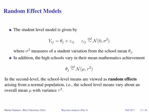
The student level model is given by

Yij = θj + εij εijiid∼ N (0, σ2)

where σ2 measures of a student variation from the school mean θj .

In addition, the high schools vary in their mean mathematics achievement

θjiid∼ N (µ, τ2)

In the second-level, the school-level means are viewed as random effectsarising from a normal population, i.e., the school level means vary about anoverall mean µ with variance τ2.


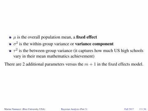
µ is the overall population mean, a fixed effectσ2 is the within-group variance or variance componentτ2 is the between-group variance (it captures how much US high schoolsvary in their mean mathematics achievement)

There are 2 additional parameters versus the m+ 1 in the fixed effects model.


Let’s look at the marginal model. Because linear combinations of normals arenormally distributed we have the equivalent model:

Yij ∼ N (µ, τ2 + σ2)

where

Cov(Yij , Yi′j) = τ2

Cov(Yij , Yi′j′) = 0 for j 6= j′

This model implies students within schools are exchangeable and studentachievements across different schools are independent given the school effect.


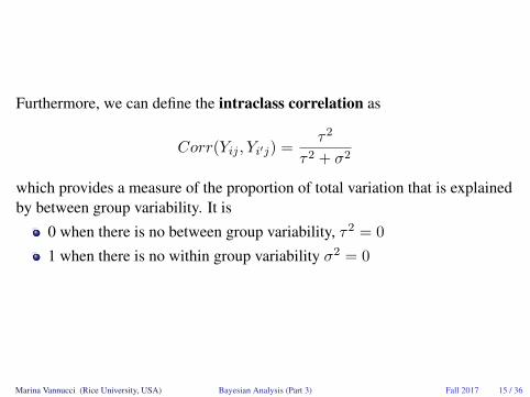
Furthermore, we can define the intraclass correlation as

Corr(Yij , Yi′j) =τ2

τ2 + σ2

which provides a measure of the proportion of total variation that is explainedby between group variability. It is

0 when there is no between group variability, τ2 = 0

1 when there is no within group variability σ2 = 0


Example (continued): Classical estimation

Find the MLE’s of µ, σ2, τ2 from the marginal model for Yij .

Use Residual Maximum Likelihood (REML): fit fixed effects by leastsquares, then estimate variance components by ML using residuals.

To fit linear mixed effect models in R, use library nlme and functionlme


fit.lme = lme(fixed = MathAch ˜ 1, random = ˜ 1 |School)summary(fit.lme)

Linear mixed-effects model fit by REML

Random effects:Formula: ˜1 | School

(Intercept) ResidualStdDev: 2.934966 6.256862

Fixed effects: MathAch ˜ 1Value Std.Error DF t-value p-value

(Intercept) 12.63697 0.2443936 7025 51.70747 0

Number of Observations: 7185Number of Groups: 160


REML Estimates

µ = 12.64

τ = 2.93 or τ2 = 8.61

σ = 6.26 or σ2 = 39.14

ρ = 8.61/(8.61 + 39.14) = 0.18

Roughly 20% of the variation in math achievement scores can be attributed todifferences among schools. The remaining variation is due to variation amongstudents within schools.


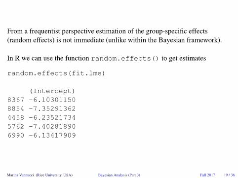
From a frequentist perspective estimation of the group-specific effects(random effects) is not immediate (unlike within the Bayesian framework).

In R we can use the function random.effects() to get estimates

random.effects(fit.lme)

(Intercept)8367 -6.103011508854 -7.352913624458 -6.235217345762 -7.402818906990 -6.13417909


Bayesian Hierarchical Model

Unknown parameters of interest: θj , µ, σ2, τ2

Distribution for θj is given by the 2nd level model specification

Yij ∼ N (θj , σ2)

θj ∼ N (µ, τ2)

(µ, σ2, τ2) ∼ p(.)

We specify priors for (µ, σ2, τ2).

Can use a default prior p(µ, σ2, τ2) ∝ 1/σ2 [a reference prior on τ2

would cause the posterior to be improper. Use p(τ2) ∝ 1]

The joint posterior distribution is given by

p(θ1, . . . , θm, µ, σ2, τ2|Y ) ∝ p(Y |θθθ, σ2)p(θθθ|µ, τ2)p(µ, σ2, τ2)


replacing variance components with precisions φ and φµ

p(Y |θj , φ) ∝∑j

∑i

φ1/2 exp(1

2φ(Yij − θj)2

)p(θj , |µ, φµ) ∝ φ1/2µ exp

(1

2φµ(θj − µ)2

)and, under the default prior,

p(µ|θj , φ, φµ, Y ) ∝∏j

p(θj |µ, φµ)p(µ) = N(∑ θj

m,

1

mφµ

)

See Hoff Chapter 8.3 for full conditionals on θj , φ, φµ (also for the moregeneral case of a Normal-Ga-Ga prior)


We cannot obtain the posterior distributions in closed form.

We can use Gibbs sampling and create a Markov chain that generatesvalues from the following full conditional distributions:

p(θj |Y, θθθ(−j), µ, σ2, τ2) for j = 1, . . . ,m

p(µ|Y, θθθ, σ2, τ2)p(σ2|Y, θθθ, µ, τ2)p(τ2|Y, θθθ, µ, σ2)


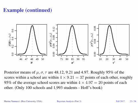
Example (continued)

46 47 48 49 50

0.0

0.2

0.4

0.6

µµ

p(µµ|

y 1...

y m)

75 80 85 90 95

0.00

0.04

0.08

0.12

σσ2

p(σσ2 |y

1...y

m)

10 20 30 40 50

0.00

0.04

0.08

ττ2

p(ττ2 |y

1...y

m)

Posterior means of µ, σ, τ are 48.12, 9.21 and 4.97. Roughly 95% of thescores within a school are within 4× 9.21 = 37 points of each other, roughly95% of the average school scores are within 4× 4.97 = 20 points of eachother. (Only 100 schools and 1,993 students - Hoff’s book)


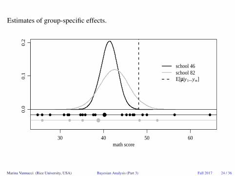
Estimates of group-specific effects.

30 40 50 60math score

0.0

0.1

0.2

● ●●● ● ●● ●● ● ●● ● ●● ●● ●● ●●●●● ●●● ●

school 46school 82E[µµ|y1...ym]


Shrinkage Effect.

E[θj |µ, τ, Y ] =nj yj/σ

2 + µ/τ2

nj/σ2 + 1/τ2

average of empirical mean yj and overall mean µ. Pulled away from yjversus µ by amount that depends on njthe larger nj the more info we have for that group, the less we need toborrow from the rest

●

●

●

●

●

●●

●●

●

●

●●

●

●●

●

●

●

●

●

●

●

●●

●

●

●

●

●●●

●

●

●

●

●

●

●

●

●

●

●

●

●

●

●

●

●

●

●

●

●

●

●

●

●

●●

●

●

●

●

●

●●

●

●

●

●

●

●

●

●

●

●

●

●

●

●

●

●

●●

●

●

●

●●

●●●

●

●

●

●

●

●

●

●

40 45 50 55 60 65

4045

5055

60

y

θθ

●●

●●

●●●

● ●

●

●

●●

●●

●

●

●

●

●

●●

●

●●●

●

●

●● ●

●●●

●●

●

●

●●

●

●

●●

●●

●●

●

●

●

●

●

●●

●

●●●

●●

●●

●●●

●

●

●

●●

●

●

●

●

●

●

●

●

●

●

●

● ●

●

●●

● ●

●●●●

● ●● ●

●●●

5 10 15 20 25 30

−4−2

02

46

8

sample size

y−−θθ


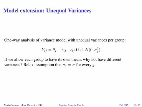
Model extension: Unequal Variances

One-way analysis of variance model with unequal variances per group:

Yij = θj + εij , εij i.i.d. N(0, σ2j )

If we allow each group to have its own mean, why not have differentvariances? Relax assumption that σj = σ for every j.


Priors:1σ2j∼ Gamma(ν0/2, ν0σ

20/2)

prior on σ20: p(σ20) ∝ 1σ20

this is equivalent to having the yij |θj , σ20, λj ∼ N(θj , σ20/λj) where

λj ∼ Gamma(ν0/2, ν0/2) so marginally the yij are multivariate t withν0 degrees of freedom with means θj and scale σ2jprior on ν0: ν0 ∼ Gamma(2, 1/2), so prior degrees of freedom 4


Full Conditionals:1σ2j| rest ∼ Gamma((ν0 + nj)/2, (ν0σ

20 +

∑(yij − θj)2))

σ20| rest ∼ Gamma((a+ Jν0)/2, (b+∑

(1/σ2j )))

ν0 no closed form full conditional


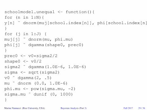
schoolmodel.unequal <- function(){for (n in 1:N){y[n] ˜ dnorm(muj[school.index[n]], phi[school.index[n]])}for (j in 1:J) {muj[j] ˜ dnorm(mu, phi.mu)phi[j] ˜ dgamma(shape0, prec0)}prec0 <- v0*sigma2/2shape0 <- v0/2sigma2 ˜ dgamma(1.0E-6, 1.0E-6)sigma <- sqrt(sigma2)v0 ˜ dgamma(2, .5)mu ˜ dnorm (0.0, 1.0E-6)phi.mu <- pow(sigma.mu, -2)sigma.mu ˜ dunif (0, 1000)}


Example (continued):

Posterior distributions of µ, τ2, σ20 .


Shrinkage of means.

E[θj |µ, τ2, σ20, Y ] = (nj/σ2j + 1/τ2)−1(

njσ2jyj +

1

τ2µ)


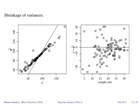
Shrinkage of variances.

●

●

●

●

●

●●

●

●

●●

●

●●

●

●

●

●

●

●

●

●

●●●

●

●

●●

●

●

●

●

●

●

●

●●●●●●

●

●

●

●

●

●

●

●

●

●

●

●

●

●

●

●

●

●

●

●

●

●

●

●

●

●

●

●

●

● ●

●

●

●

●●

●

●

●●

●

●●

●

●●●

●

●●●

●

●

●

●

●

●

●

50 100 150

60

80

10

01

20

14

0

s2

σσ2

●

●

●

●

●

●●

●

●

●

●

●

●

●

●

●

●

●

●

●

●

●

●●●

●

●

●●

●

●

●

●

●

●

●

●

●

●●

●●

●

●

●

●

●

●

●

●

●

●

●

●

●

●

●

●

●

●

●

●

●

●

●

●

●

●

●

●

●

●

●

●

●

●

●

●

●

●

●

●

●

●●

●

●● ●

●

●● ●

●

●

●

●

●

●

●

5 10 15 20 25 30−

30

−1

00

10

20

30

sample size

s2−−

σσ2


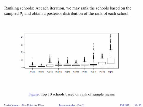
Ranking schools: At each iteration, we may rank the schools based on thesampled θj and obtain a posterior distribution of the rank of each school.

Figure: Top 10 schools based on rank of sample means


Mixed effect models

We can write θj = µ+ δj where each school mean is centered at theoverall mean µ plus some normal random effect δj .

Substituting this into the distribution for Yij , we get

Yij = µ+ δj + εij εij ∼ N (0, σ2)

withfixed effect, µschool level random effects, δjindividual random effects εij

This leads to a mixed effects model.


Yij = µ+ δj + εij

The parameters of this model are not identifiable: adding 42 to θj andsubtracting 42 from δj , leads to a new θj and δj , but the same likelihood.

Model is identifiable with the addition of the prior distributions

leads to different full conditional distributions

but this model has very poor mixing!


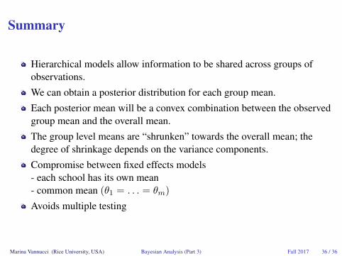
Summary

Hierarchical models allow information to be shared across groups ofobservations.

We can obtain a posterior distribution for each group mean.

Each posterior mean will be a convex combination between the observedgroup mean and the overall mean.

The group level means are “shrunken” towards the overall mean; thedegree of shrinkage depends on the variance components.

Compromise between fixed effects models- each school has its own mean- common mean (θ1 = . . . = θm)

Avoids multiple testing


stat 425: introduction to bayesian analysismarina/stat425/part3_hm.pdf1 when there is no within...

Documents