stat 305: chapter 5 - github pages

STAT 305: Chapter 5STAT 305: Chapter 5

Part IIPart II

Amin ShiraziAmin Shirazi

Course page:Course page:ashirazist.github.io/stat305.github.ioashirazist.github.io/stat305.github.io

1 / 651 / 65

https://ashirazist.github.io/stat305.github.io/

Discrete Random VariablesDiscrete Random Variables

Meaning, Use, and Common DistributionsMeaning, Use, and Common Distributions

2 / 652 / 65

GeneralInfo

Reminder:RVs

General Info About Discrete RVs

Reminder: What is a Random Variable?

Random Variables, we have already defined, take real-numbered ( ) values based on outcomes of a randomexperiment.

If we know the outcome, we know the value of therandom variable (so that isn't the random part).However, before we perform the experiment we donot know the outcome - we can only make statementsabout what the outcome is likely to be (i.e., we make"probabilistic" statements).In the same way, we do not know the value of therandom variable before the experiment, but we canmake probability statements about what value the RVmight take.

R

3 / 65

GeneralInfo

Reminder:RVs

Discrete?

Terms &Notation

Common Terms and Notation for Discrete RVs

Of course, we can't introduce a sort of new conceptwithout introducing a whole lot of new terminology.

We use capital letters to refer to discrete randomvariables: , , , ...

We use lower case letters to refer to values the discreteRVs can take: , , , , ...

While we can use to refer to the probabilitythat the discrete random variable takes the value , weusually use what we call the probability function:

For a discrete random variable , the probabilityfunction takes the value

In otherwords, we just write instead of .

X Y Z

x x1 y z

P(X = x)x

Xf(x) P(X = x)

f(x)P(X = x)

4 / 65

GeneralInfo

Reminder:RVs

Discrete?

Terms &Notation

Common Terms and Notation for Discrete RVs

We also have another function related to the probabilities,called the cumulative probability function.

For a discrete random variable taking values the CDF or cumulative probability function of , ,is defined as

Which in other words means that for any value ,

and

X x1, x2, . . .X F(x)

F(x) = ∑z≤x

f(z)

x

f(x) = P(X = x)

F(x) = P(X ≤ x)

5 / 65

GeneralInfo

Reminder:RVs

Discrete?

Terms &Notation

Common Terms and Notation for Discrete RVs (cont)

The values that can take and the probabilities attachedto those values are called the probability distribution of

(since we are talking about how the total probability 1gets spread out on (or distributed to) the values that cantake).

Example

Suppose that the we roll a die and let be the number ofdots facing up. Define the probability distribution of .Find and .

X

XX

TT

f(3) F(6)

6 / 65

GeneralInfo

Reminder:RVs

Discrete?

Terms &Notation

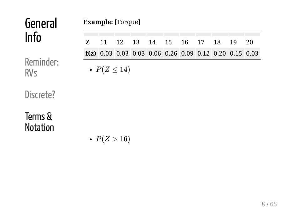
Example: [Torque]

Let the torque, rounded to the nearest integer,required to loosen the next bolt on an apparatus.

Z 11 12 13 14 15 16 17 18 19 20

f(z) 0.03 0.03 0.03 0.06 0.26 0.09 0.12 0.20 0.15 0.03

Calculate the following probabilities:

Z =

P(Z ≤ 14)

P(Z > 16)

P(Z is even)

P(Z ∈ {15, 16, 18})

7 / 65

GeneralInfo

Reminder:RVs

Discrete?

Terms &Notation

Example: [Torque]

Z 11 12 13 14 15 16 17 18 19 20

f(z) 0.03 0.03 0.03 0.06 0.26 0.09 0.12 0.20 0.15 0.03

P(Z ≤ 14)

P(Z > 16)

8 / 65

GeneralInfo

Reminder:RVs

Discrete?

Terms &Notation

Example: [Torque]

Z 11 12 13 14 15 16 17 18 19 20

f(z) 0.03 0.03 0.03 0.06 0.26 0.09 0.12 0.20 0.15 0.03

P(Z is even)

P(Z ∈ {15, 16, 18})

9 / 65

GeneralInfo

Reminder:RVs

Discrete?

Terms &Notation

More on CDF

The cumulative probability distribution (cdf) fora random variable is a function thatfor each number gives the probability that takes that value or a smaller one,

.

Since (for discrete distributions) probabilities arecalculated by summing values of ,

X F(x)x X

F(x) = P [X ≤ x]

f(x)

F(x) = P [X ≤ x] = ∑y≤x

f(y)

10 / 65

GeneralInfo

Reminder:RVs

Discrete?

Terms &Notation

More on CDF

Properties of a mathematically valid cumulativedistribution function:

for all real numbers

is monotonically increasing

is right continuous

and

This means that for any CDF

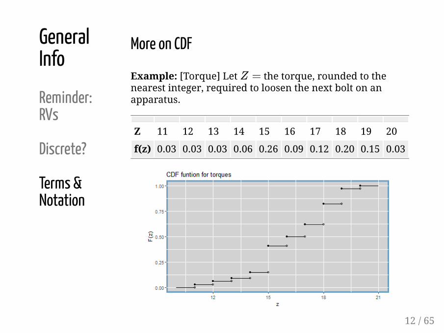
In the discrete cases, the graph of will ben stair-step graph with jumps at possible valuesof our random variable and height equal to theprobabilities associated with those values

F(x) ≥ 0 x

F(x)

F(x)

limx→−∞ F(x) = 0 limx→+∞ F(x) = 1

0 ≤ F(x) ≤ 1

F(x)

11 / 65

GeneralInfo

Reminder:RVs

Discrete?

Terms &Notation

More on CDF

Example: [Torque] Let the torque, rounded to thenearest integer, required to loosen the next bolt on anapparatus.

Z 11 12 13 14 15 16 17 18 19 20

f(z) 0.03 0.03 0.03 0.06 0.26 0.09 0.12 0.20 0.15 0.03

Z =

12 / 65

GeneralInfo

Reminder:RVs

Discrete?

Terms &Notation

More on CDF

Calculate the following probabilities using the cdf only:

F(10.7)

P(Z ≤ 15.5)

P(12.1 < Z ≤ 14)

P(15 ≤ Z < 18)

13 / 65

GeneralInfo

Reminder:RVs

Discrete?

Terms &Notation

More on CDF

One more example

Say we have a random variable with pmf:

q f(q)

1 0.34

2 0.10

3 0.22

7 0.34

Draw the CDF

Q

14 / 65

GeneralInfo

Reminder:RVs

Discrete?

Terms &Notation

Summaries

Almost all of the devices for describing relative frequency(empirical) distributions in Ch. 3 have versions that candescribe (theoretical) probability distributions.

1. Measures of location == Mean

2. Measures of spread == variance

3. Histogram == probability histograms based ontheoretical probabilities

15 / 65

MeanMean

andand

VarianceVariance

of Discrete Random Variablesof Discrete Random Variables

16 / 6516 / 65

GeneralInfo

Reminder:RVs

Discrete?

Terms &Notation

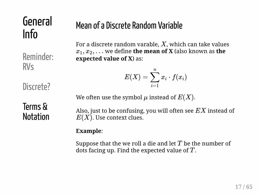
Mean of a Discrete Random Variable

For a discrete random varable, , which can take values we define the mean of X (also known as the

expected value of X) as:

We often use the symbol instead of .

Also, just to be confusing, you will often see instead of. Use context clues.

Example:

Suppose that the we roll a die and let be the number ofdots facing up. Find the expected value of .

Xx1, x2, . . .

E(X) =n

∑i=1

xi ⋅ f(xi)

μ E(X)

EXE(X)

TT

17 / 65

GeneralInfo

Reminder:RVs

Discrete?

Terms &Notation

Variance of a Discrete Random Variable

For a discrete random varable, , which can take values and has mean we define the variance of

as:

There are other usefule ways to write this, mostimportantly:

which is the same as

Xx1, x2, . . . μ X

V ar(X) =n

∑i=1

(xi − μ)2 ⋅ f(xi)

V ar(X) =n

∑i=1

x2i

⋅ f(xi) − μ2

VarX = ∑x

(x − EX)2f(x) = E(X2) − (EX)2.

18 / 65

GeneralInfo

Reminder:RVs

Discrete?

Terms &Notation


Example:

Suppose that the we roll a die and let be the number ofdots facing up. What is the variance of ?

T

T

19 / 65

GeneralInfo

Reminder:RVs

Discrete?

Terms &Notation


Example

Say we have a random variable with pmf:

q f(q)

1 0.34

2 0.10

3 0.22

7 0.34

Find the variance and standard deviation

Q

20 / 65

GeneralInfo

Reminder:RVs

Discrete?

Terms &Notation

Summary

Discrete Random Variables

Discrete RVs are RVs that will take one of a countableset of values.

When working with a discrete random variable, it iscommon to need or use the RV's

probability distribution: the values the RV cantake and their probabilities

probability function: a function where

cumulative probability function: a function where.

mean: a value for defined by

variance: a value for defined by

f(x) = P(X = x)

F(x) = P(X ≤ x)

XEX = ∑

xx ⋅ f(x)

XV arX = ∑x(x − μ)2 ⋅ f(x) 21 / 65

Your Turn:Your Turn:

Chapter 5 Handout 1Chapter 5 Handout 1

22 / 6522 / 65

Common DistributionsCommon DistributionsWorking with O� The Shelf Random VariablesWorking with O� The Shelf Random Variables

23 / 6523 / 65

GeneralInfo

CommonDistributions

Background

Common Distributions

Why Are Some Distributions Worth Naming?

Even though you may create a random variable in aunique scenario, the way that it's probability distributionbehaves (mathematically) may have a lot in common withother random variables in other scenarios. For instance,

I roll a die until I see a 6 appear and then stop. Icall the number of times I have to roll the diein total.

I flip a coin until I see heads appear and thenstop. I call the number of times I have to flipthe coin in total.

I apply for home loans until I get accepted andthen I stop. I call the number of times I haveto apply for a loan in total.

X

Y

Z

24 / 65

GeneralInfo

CommonDistributions

Background

Why Are Some Distributions Worth Naming? (cont)

In each ot the above cases, we count the number of timeswe have to do some action until we see some specificresult. The only thing that really changes from the randomvariables perspective is the likelyhood that we see thespecific result each time we try.

Mathematically, that's not a lot of difference. And if we canreally understand the probability behavior of one of thesescenarios then we can move our understanding to thedifferent scenario pretty easily.

By recognizing the commonality between these scenarios,we have been able to identify many random variables thatbehave very similarly. We describe the similarity in theway the random variables behave by saying that they havea common/shared distribution.

We study the most useful ones by themselves.

25 / 65

The Bernoulli DistributionThe Bernoulli Distribution

26 / 6526 / 65

GeneralInfo

CommonDistributions

Background

Bernoulli

The Bernoulli Distribution

Origin: A random experiment is performed that results inone of two possible outcomes: success or failure. Theprobability of a successful outcome is .

Definition: takes the value 1 if the outcome is a success. takes the value 0 if the outcome is a failure.

probability function:

which can also be written as

p

XX

f(x) =⎧⎨⎩

p x = 1,1 − p x = 0,0 o. w.

‘

f(x) = { px(1 − p)1−x x = 0, 1

0 o. w.‘

27 / 65

Bernoulli DistributionBernoulli DistributionExpected Value and VarianceExpected Value and Variance

28 / 6528 / 65

GeneralInfo

CommonDistributions

Background

Bernoulli


Expected value: E(X) = p

29 / 65

GeneralInfo

CommonDistributions

Background

Bernoulli


Variance: V ar(X) = (1 − p) ⋅ p

30 / 65

GeneralInfo

CommonDistributions

Background

Bernoulli


A few useful notes:

In order to say that " has a bernoulli distributionwith success probability " we write

Trials which results in which the only possibleoutcomes are "success" or "failure" are calledBernoulli Trials

The value is the Bernoulli distribution's parameter.We don't treat parameters like random values - theyare fixed, related to the real process we are studying.

"Success" does not mean something we wouldperceive as "good" has happened. It just means theoutcome we were watching for was the outcome wegot.

Please note: we have two outcomes, but theprobability for each outcome is not the same (duh!).

Xp

X ∼ Bernoulli(p)

p

31 / 65

The Binomial DistributionThe Binomial Distribution

32 / 6532 / 65

CommonDistributions

Background

Bernoulli

Binomial

The Binomial Distribution

Origin: A series of independent random experiments, ortrials, are performed. Each trial results in one of twopossible outcomes: successful or failure. The probability ofa successful outcome, , is the same across all trials.

Definition: For trials, is the number of trials with asuccessful outcome. can take values .


With ,

`

where and .

n

p

n XX 0, 1, … , n

0 < p < 1

f(x) =⎧⎨⎩

px(1 − p)n−x x = 0, 1, … , n

0 o. w.

n!

x!(n − x)!

n! = n ⋅ (n − 1) ⋅ (n − 2) ⋅ … ⋅ 1 0! = 1

33 / 65

CommonDistributions

Background

Bernoulli

Binomial

Examples of Binomial Distribution

Number of hexamine pallets in a batch of total pallets made from a

palletizing machine that conform to somestandard.

Number of runs of the same chemicalprocess with percent yield above giventhat you run the process 1000 times.

Number of winning lottery tickets whenyou buy 10 tickets of the same kind.

n = 50

80

34 / 65

CommonDistributions

Background

Bernoulli

Binomial

35 / 65

CommonDistributions

Background

Bernoulli

Binomial


Plots of Binomial distribution based on different successprobabilities and sample sizes.

36 / 65

CommonDistributions

Background

Bernoulli

Binomial


Example [10 component machine]

Suppose you have a machine with 10 independentcomponents in series. The machine only works if all thecomponents work. Each component succeeds withprobability and fails with probability

.

Let be the number of components that succeed in agiven run of the machine. Then

Question: what is the probability of the machine workingproperly?

p = 0.951 − p = 0.05

Y

Y ∼ Binomial(n = 10, p = 0.95)

37 / 65

CommonDistributions

Background

Bernoulli

Binomial



What if I arrange these 10 components in parallel? Thismachine succeeds if at least 1 of the components succeeds.

What is the probability that the new machine succeeds?

Y ∼ Binomial(n = 10, p = 0.95)

38 / 65

Binomial DistributionBinomial DistributionExpected Value and VarianceExpected Value and Variance

39 / 6539 / 65

CommonDistributions

Background

Bernoulli

Binomial


Expected value:

Variance:

E(X) = n ⋅ p

V ar(X) = n ⋅ (1 − p) ⋅ p

40 / 65

CommonDistributions

Background

Bernoulli

Binomial



Calculate the expected number of components to succeedand the variance.

41 / 65

CommonDistributions

Background

Bernoulli

Binomial


A few useful notes:

In order to say that " has a binomial distributionwith trials and success probability " we write

If are independent Bernoullirandom variables with the same then

is a binomial randomvariable with trials and success probability .

Again, and are referred to as "parameters" for theBinomial distribution. Both are considered fixed.

Don't focus on the actual way we got the expectedvalue - focus on the trick of trying to get part of yourcomplicated summation to "go away" by turning it intothe sum of a probability function.

Xn p

X ∼ Binomial(n, p)

X1, X2, … , Xn np

X = X1 + X2 + … + Xn

n p

n p

42 / 65

The Geometric DistributionThe Geometric Distribution

43 / 6543 / 65

CommonDistributions

Background

Bernoulli

Binomial

Geometric

The Geometric Distribution

Origin: A series of independent random experiments, ortrials, are performed. Each trial results in one of twopossible outcomes: successful or failure. The probability ofa successful outcome, , is the same across all trials. Thetrials are performed until a successful outcome isobserved.

Definition: is the trial upon which the first successfuloutcome is observed. can take values .


With ,

p

XX 1, 2, …

0 < p < 1

f(x) = { p(1 − p)x−1 x = 1, 2, . . .

0 o. w.‘

44 / 65

CommonDistributions

Background

Bernoulli

Binomial

Geometric

Examples of Geometric Distribution

Number of rolls of a fair die until you landa 5

Number of shipments of raw materials youget until you get a defective one (successdoes not need to have positive meaning)

Number of car engine starts untill thebattery dies.

45 / 65

CommonDistributions

Background

Bernoulli

Binomial

Geometric

Shape of Geometric Distribution

The probability of observing the first successdecreases as the number of trialsincreases(even at a faster rate as increases)p

46 / 65

CommonDistributions

Background

Bernoulli

Binomial

Geometric


Cumulative probability function:

Here's how we get that cumulative probability function:

The probability of a failed trial is .The probability the first trial fails is also just .The probability that the first two trials both fail is

.The probability that the first trials all fail is .This gets us to this math:

F(x) = 1 − (1 − p)x

1 − p1 − p

(1 − p) ⋅ (1 − p) = (1 − p)2

x (1 − p)x

F(x) = P(X ≤ x)

= 1 − P(X > x)

= 1 − (1 − p)x

47 / 65

MeanMean

andand

VarianceVariance

of Geometric Distrbutionof Geometric Distrbution

48 / 6548 / 65

CommonDistributions

Background

Bernoulli

Binomial

Geometric


Expected value:

Variance:

E(X) =1

p

V ar(X) =1 − p

p2

49 / 65

CommonDistributions

Background

Bernoulli

Binomial

Geometric

Example

NiCad batteries: An experimental program wassuccessful in reducing the percentage of manufacturedNiCad cells with internal shorts to around . Let bethe test number at which the first short is discovered.Then, .

Calculate

1% T

T ∼ Geom(p)

P(1st or 2nd cell tested has the 1st short)

P(at least 50 cells tested without finding a short)

50 / 65

CommonDistributions

Background

Bernoulli

Binomial

Geometric

Example

NiCad batteries:

Calculate the expected test number at which the first shortis discovered and the variance in test numbers at whichthe first short is discovered.

51 / 65

CommonDistributions

Background

Bernoulli

Binomial

Geometric

Example

A shipment of 200 widgets arrives from a new widgetdistributor. The distributor has claimed that the widgetsthere is only a 10% defective rate on the widgets. Let bethe random variable asociated with the number of trialsuntill finding the first defective widgets.

What is the probability distribution associated withthis random variable ? Precisely specify theparameter(s).

How many widgets would you expect to test beforefinding the first defective widget?

X

X

52 / 65

CommonDistributions

Background

Bernoulli

Binomial

Geometric

Example

You find your first defective widget while testing the thridwidget.

What is the probability that a the first defective widgetwould be found on the third test if there are only 10%defective widgets from in the shipment?

P(x = 3) = p(1 − p)x−1

= 0.1(1 − 0.1)3−1

= 0.1(0.9)2 = 0.081

53 / 65

CommonDistributions

Background

Bernoulli

Binomial

Geometric

Example

What is the probability that a the first defective widgetwould be found by the third test if there are only 10%defective widgets from in the shipment?

P(x ≤ 3) = FX(3) = 1 − (1 − p)3

= 1 − (1 − .1)3

= 1 − (0.9)3 = 0.271

54 / 65

The Poisson DistributionThe Poisson Distribution

55 / 6555 / 65

CommonDistributions

Background

Bernoulli

Binomial

Geometric

Poisson

The Poisson Distribution

Origin: A rare occurance is watched for over a specifiedinterval of time or space.

It's often important to keep track of the total number ofoccurrences of some relatively rare phenomenon.

Definition

Consider a variable

X : the count of occurences of a phenomenonacross a specified interval of time or space

or

X: the number of times the rare occurance isobserved

56 / 65

CommonDistributions

Background

Bernoulli

Binomial

Geometric

Poisson



The Poisson$(\lambda)$ distribution is a discreteprobability distribution with pmf

For

f(x) =

⎧⎪ ⎪⎨⎪ ⎪⎩

x = 0, 1, . . .

0 o. w.

e−λλx

x!

λ > 0

57 / 65

CommonDistributions

Background

Bernoulli

Binomial

Geometric

Poisson


These occurrences must:

be independentbe sequential in time ( no two occurances at once)occur at the same constant rate

the rate parameter, is the expected number ofoccurances in the specified interval of time or space (i.e

)

λ

λ

E(X) = λ

58 / 65

CommonDistributions

Background

Bernoulli

Binomial

Geometric

Poisson


Examples that could follow a Poisson$(\lambda)$distribution :

is the number of shark attacks off the coastof CA next year, attacks per year

is the number of shark attacks off the coastof CA next month, attacks permonth

is the number of -particles emitted from asmall bar of polonium, registered by a counterin a minute, particles per minute

is the number of particles per hour, particles per

hour.

Y

λ = 100

Z

λ = 100/12

N α

λ = 459.21

J

λ = 459.21 ∗ 60 = 27, 552.6

59 / 65

CommonDistributions

Background

Bernoulli

Binomial

Geometric

Poisson


Right skewed with peak near λ

60 / 65

CommonDistributions

Background

Bernoulli

Binomial

Geometric

Poisson


For a Poisson$(\lambda)$ random variable,X

μ = EX =∞

∑x=0

x = λ

σ2 = VarX =∞

∑x=0

(x − λ)2 = λ

e−λλx

x!

e−λλx

x!

61 / 65

CommonDistributions

Background

Bernoulli

Binomial

Geometric

Poisson

Example

Arrivals at the library

Some students' data indicate that between 12:00 and12:10pm on Monday through Wednesday, an average ofaround 125 students entered Parks Library at ISU.Consider modeling

M : the number of students entering the ISUlibrary between 12:00 and 12:01pm nextTuesday

Model . What would a reasonable choiceof be?

M ∼ Poisson(λ)λ

62 / 65

CommonDistributions

Background

Bernoulli

Binomial

Geometric

Poisson

Example

Arrivals at the library

Under this model, the probability that between and students arrive at the library between 12:00 and 12:01 PMis:

10 15

63 / 65

CommonDistributions

Background

Bernoulli

Binomial

Geometric

Poisson

Shark attacks

Let be the number of unprovoked shark attacks thatwill occur off the coast of Florida next year. Model

From the shark data athttp://www.flmnh.ufl.edu/fish/sharks/statistics/FLactivity.htm,246 unprovoked shark attacks occurred from 2000 to 2009.

What would a reasonable choice of be?

X

X ∼ Poisson(λ).

λ

64 / 65

http://www.flmnh.ufl.edu/fish/sharks/statistics/FLactivity.htm

CommonDistributions

Background

Bernoulli

Binomial

Geometric

Poisson

Shark attacks

Under this model, calculate the following:

P(no attacks next year)

P(at least 5 attacks)

P(more than 10 attacks)

65 / 65

stat 305: chapter 5 - github pages

Documents