stat 270 - chapter 5 continuous distributionssgolchi/stat-270/stat270ch5.pdf · stat 270 - chapter...

STAT 270 - Chapter 5Continuous Distributions

June 27, 2012

Shirin Golchi () STAT270 June 27, 2012 1 / 59

Continuous rv’s

Definition: X is a continuous rv if it takes values in an interval, i.e., rangeof X is continuous.e.g. Temprature in degrees celcius in class.Definition: Probability density function (pdf) or density of continuous arv X , fX (x) ≥ 0 is such that:

P(a ≤ X ≤ b) =

∫ b

afX (x)dx

for all a < b.From definition:

P(X = c) =

∫ c

cfX (x)dx = 0

for all c ∈ <.


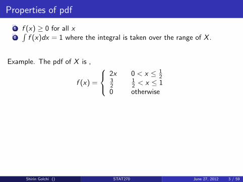
Properties of pdf

1 f (x) ≥ 0 for all x2∫f (x)dx = 1 where the integral is taken over the range of X .

Example. The pdf of X is ,

f (x) =

2x 0 < x ≤ 1

232

12 < x ≤ 1

0 otherwise


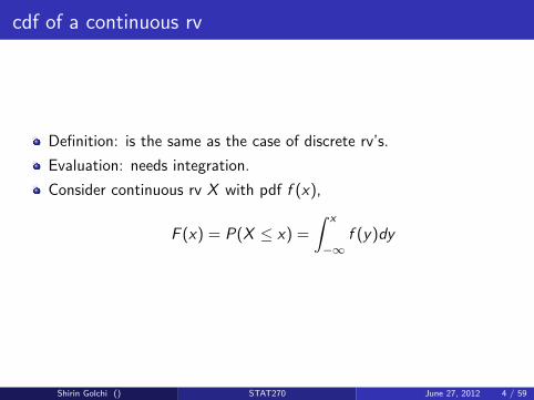
cdf of a continuous rv

Definition: is the same as the case of discrete rv’s.

Evaluation: needs integration.

Consider continuous rv X with pdf f (x),

F (x) = P(X ≤ x) =

∫ x

−∞f (y)dy


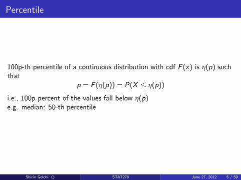
Percentile

100p-th percentile of a continuous distribution with cdf F (x) is η(p) suchthat

p = F (η(p)) = P(X ≤ η(p))

i.e., 100p percent of the values fall below η(p)e.g. median: 50-th percentile


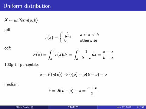
Uniform distribution

X ∼ uniform(a, b)

pdf:

f (x) =

{1

b−a a < x < b

0 otherwise

cdf:

F (x) =

∫ x

af (x)dx =

∫ x

a

1

b − adx =

x − a

b − a

100p-th percentile:

p = F (η(p))⇒ η(p) = p(b − a) + a

median:

x̃ = .5(b − a) + a =a + b

2


Example (5.1, 5.3)

f (x) =

x 0 < x ≤ 112 1 < x ≤ 20 otherwise

F (x) =

η(p) =


Expectation

Definition is the same as the case of discrete rv’sIn claculation the sum is replaced by integral:X continuous rv with pdf f (x)

E (X ) =

∫xxf (x)dx

where the integral is taken over the range of X .


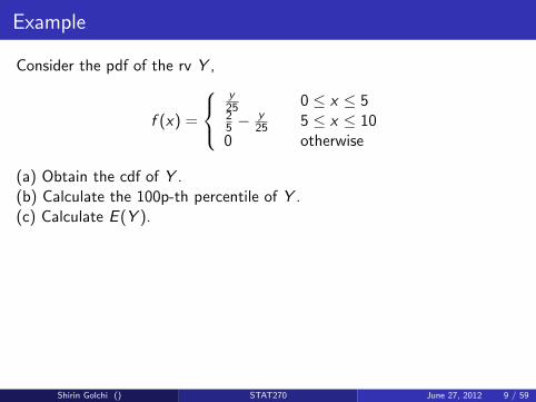
Example

Consider the pdf of the rv Y ,

f (x) =

y25 0 ≤ x ≤ 525 −

y25 5 ≤ x ≤ 10

0 otherwise

(a) Obtain the cdf of Y .(b) Calculate the 100p-th percentile of Y .(c) Calculate E (Y ).


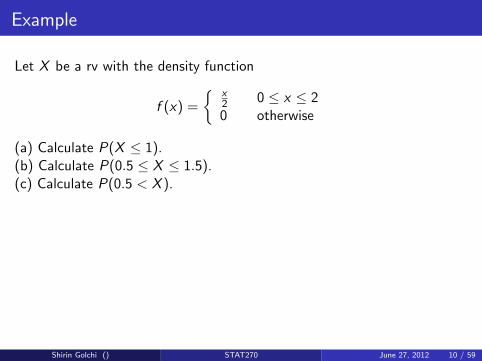
Example

Let X be a rv with the density function

f (x) =

{x2 0 ≤ x ≤ 20 otherwise

(a) Calculate P(X ≤ 1).(b) Calculate P(0.5 ≤ X ≤ 1.5).(c) Calculate P(0.5 < X ).


Example

Suppose I never finish the lectures before the end of the hour and alwaysfinish within two minutes after the hour. Let X be the time that elapsesbetween the end of the hour and the end of the lecture and suppose thepdf of X is

f (x) =

{kx2 0 ≤ x ≤ 20 otherwise

(a) Evalaute k.(b) What is the probability that the lecture ends within one minute of theend of the hour?(c) What is the probability that the lecture continues beyond the hour forbetween 60 and 90 seconds?(d) What is the probability that the lecture continues for at least 90seconds beyond the end of the hour?


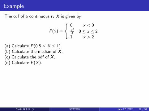
Example

The cdf of a continuous rv X is given by

F (x) =

0 x < 0x2

4 0 ≤ x ≤ 21 x > 2

(a) Calculate P(0.5 ≤ X ≤ 1).(b) Calculate the median of X .(c) Calculate the pdf of X .(d) Calculate E (X ).


Expectation and variance

Expectation of a continuous rv X with pdf f (x) is

µ = E (X ) =

∫xf (x)dx

where the integral is taken over the range of X .

Expectation of a function of X , g(X ), is given by

E (g(X )) =

∫g(x)f (x)dx

. Variance of a continuous rv X is given by

σ2 = var(X ) = E (X − E (X ))2 =

∫(x − E (X ))2f (x)dx

var(X ) = E (X 2)− (E (X ))2


The Normal/Gaussian/bell-shaped distribution

The most important distribution of all!

Widely applicable to statistical science problems

Mathematically elegant

Definition: X ∼ Normal(µ, σ2) if the pdf of X is given by

f (x) =1√

2πσ2e−

12

( x−µσ

)2

where −∞ < x <∞, −∞ < µ <∞ and σ > 0.


Important notes on the Gaussian distribution

Family of distributions indexed by parameters µ and σ2.

Symmetric about µ: f (µ+ δ) = f (µ− δ), for all δ.

f (x) decreases exponentially as x → −∞ and x →∞, but it nevertouches 0.

f (x) in intractable:∫ ba f (x)dx has to be approximated using

numerical methods.


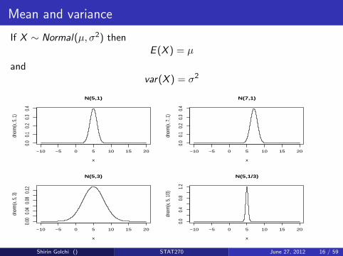
Mean and variance

If X ∼ Normal(µ, σ2) thenE (X ) = µ

andvar(X ) = σ2

−10 −5 0 5 10 15 20

0.0

0.1

0.2

0.3

0.4

N(5,1)

x

dnor

m(x

, 5, 1

)

−10 −5 0 5 10 15 20

0.0

0.1

0.2

0.3

0.4

N(7,1)

x

dnor

m(x

, 7, 1

)

−10 −5 0 5 10 15 20

0.00

0.04

0.08

0.12

N(5,3)

x

dnor

m(x

, 5, 3

)

−10 −5 0 5 10 15 20

0.0

0.4

0.8

1.2

N(5,1/3)

x

dnor

m(x

, 5, 1

/3)


The standard normal distribution

Probabilities are obtained through normal tables

Choice of µ and σ does not restrict us in calculation of probabilities:any normal distribution can be converted into the standard normaldistribution: Z ∼ Normal(0, 1),

f (z) =1√2π

e−z2

2

Normal tables provide cumulative probabilities for the standardnormal variable.


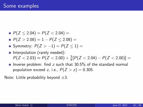
Some examples

P(Z ≤ 2.04) = P(Z < 2.04) =

P(Z > 2.08) = 1− P(Z ≤ 2.08) =

Symmetry: P(Z > −1) = P(Z ≤ 1) =

Interpolation (rarely needed):P(Z < 2.03) ≈ P(Z < 2.00) + 3

4 [P(Z < 2.04)− P(Z < 2.00)] =

Inverse problem: find z such that 30.5% of the standard normalpopulation exceed z , i.e., P(Z > z) = 0.305.

Note: Little probability beyond ±3.


Some useful Z-values

z 1.282 1.645 1.96 2.326 2.576

f(z) 0.9 0.95 0.975 0.99 0.995

Transformation to the standard normal distribution:

IfX ∼ Normal(µ, σ2)

then

Z =X − µσ

∼ Normal(0, 1)


Example

A subset of Canadians watch an average of 6 hours of TV every day. If theviewing times are normally distributed with sd of 2.5 hours. What is theprobability that a randomly selected person from thet population watchesmore than 8 hours of TV per day?


Example

The substrate concentration (mg/cm3) of influent to a reactor is normallydistrbuted with µ = 0.4 and σ = 0.05.(a) What is the probability that the concentration exceeds 0.35?(b) What is the probability that the concentration is at most 0.2?(c) How would you characterize the largest 5% of all concentration values?


More examples ...


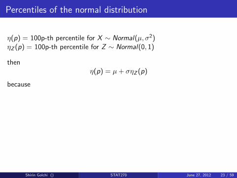
Percentiles of the normal distribution

η(p) = 100p-th percentile for X ∼ Normal(µ, σ2)ηZ (p) = 100p-th percentile for Z ∼ Normal(0, 1)

thenη(p) = µ+ σηZ (p)

because


Example

Find the 86.43th percentile of the Normal(3,25).


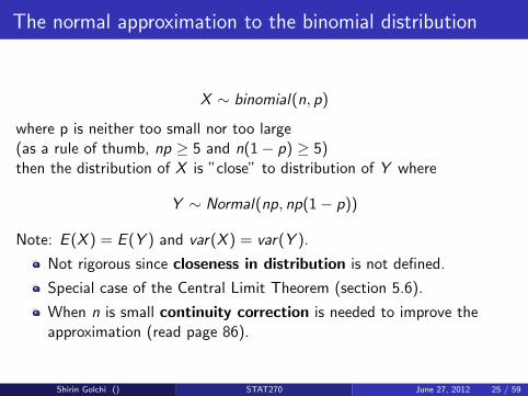
The normal approximation to the binomial distribution

X ∼ binomial(n, p)

where p is neither too small nor too large(as a rule of thumb, np ≥ 5 and n(1− p) ≥ 5)then the distribution of X is ”close” to distribution of Y where

Y ∼ Normal(np, np(1− p))

Note: E (X ) = E (Y ) and var(X ) = var(Y ).

Not rigorous since closeness in distribution is not defined.

Special case of the Central Limit Theorem (section 5.6).

When n is small continuity correction is needed to improve theapproximation (read page 86).


Example

Let X ∼ binomial(100, 0.5) and Y ∼ Normal(50 = np, 25 = np(1− p)).

P(X ≥ 60) =∑100

x=60

(100x

)(0.5)x(0.5)(100−x) = 0.017

P(Y ≥ 60) = P(Z ≥ 60−505 ) = 1− P(Z ≤ 2) = 0.022


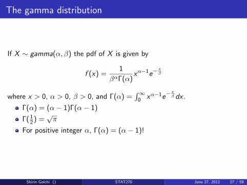
The gamma distribution

If X ∼ gamma(α, β) the pdf of X is given by

f (x) =1

βαΓ(α)xα−1e−

xβ

where x > 0, α > 0, β > 0, and Γ(α) =∫∞

0 xα−1e−xβ dx .

Γ(α) = (α− 1)Γ(α− 1)

Γ( 12 ) =

√π

For positive integer α, Γ(α) = (α− 1)!


The gamma distribution

Used to model right-skewed continuous data

Family of distributions indexed by parameters α and β.

Intractable except for particular values of α and β.

E (X ) = αβ and var(X ) = αβ2

Proof:


The exponential distribution

If X ∼ exponential(λ) the pdf of X is given by

f (x) = λe−λx

where x > 0 and λ > 0.

0 1 2 3 4 5

0.00.2

0.40.6

0.81.0

EXP(1)

x

f(x)


The exponential distribution

Family of distributions indexed by the parameter λ.

Special case of the gamma distribution where α = 1 and β = 1λ .

(1-parameter sub-family of the gamma family)

E (X ) = 1λ and var(X ) = 1

λ2

cdf:

F (x) = P(X ≤ x) =

∫ x

0λe−λydy = 1− e−λx

where x > 0.


Memoryless property

An old light bulb is just as good as a new one!

Let X ∼ exponential(λ) be the life span in hours of a light bulb . What isthe probability that it lasts a + b hours given that it has lasted a hours?

P(X > a + b|X > a) = P(X > b)

Proof:

Do you believe this about light bulbs?


The relationship between the Poisson and exponentialdistributions

NT : Number of events occurring in the time interval (0,T )

NT ∼ Poisson(λT )

X : Waiting time until the first event occurs

cdf of X :F (x) = 1− e−λx

i.e.,X ∼ exponential(λ)


Example 5.14


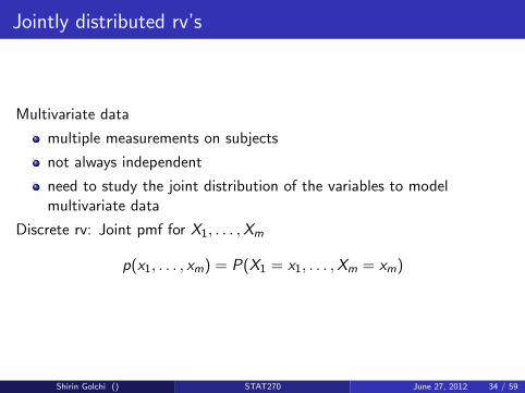
Jointly distributed rv’s

Multivariate data

multiple measurements on subjects

not always independent

need to study the joint distribution of the variables to modelmultivariate data

Discrete rv: Joint pmf for X1, . . . ,Xm

p(x1, . . . , xm) = P(X1 = x1, . . . ,Xm = xm)


Example 1

Suppose X and Y have a joint pmf given by the following table

X = 1 X = 2 X = 3

Y = 1 .1 .5 .1Y = 2 .05 .1 .15

P(X = 3,Y = 2) =P(X < 3,Y = 1) =Sum out the nuisance parameter X to obtain the marginal pmf of Y:p(Y = 1) =Verify that this is a joint pmf:

Read page 91.


Continuous rv’s

Joint pdf of X1, . . . ,Xm, f (x1, . . . , xm) is such that

f (x1, . . . , xm) ≥ 0 for all x1, . . . , xm.∫ ∫. . .∫f (x1, . . . , xm)dx1dx2 . . . dxm = 1 where the integral is taken

over the range of X1, . . . ,Xm.

The probability of event A is given by

P((X1, . . . ,Xm) ∈ A) =

∫ ∫. . .

∫Af (x1, . . . , xm)dx1 . . . dxm

Marginal pdf’s are obtained by integrating out the nuisance variables.


Example 2

Let X and Y have the joint pdf f (x , y) = 27 (x + 2y) where 0 < x < 1 and

1 < y < 2.(a) Calculate P(X ≤ 1

2 ,Y ≤32 ).

(b) Obtain f (y).

Read Example 5.15.


Example 3 (dependence in range)

Let X and Y have the joint pdf

f (x) =

{3y 0 ≤ x ≤ y ≤ 10 otherwise

Calculate P(Y ≤ 23 ).

Read Example 5.16.


Independent random variables

X and Y discrete independent rv’s:

p(x , y) = p(x)p(y)

X and Y continuous rv’s:

f (x , y) = f (x)f (y)

Example: Independent bivariate normal distribution

f (x , y) =1

2πσ1σ2exp {−1

2(

(x − µ1)2

σ21

+(y − µ2)2

σ22

)} = f (x)f (y)

where X ∼ N(µ1, σ21) and Y ∼ N(µ2, σ

22).

Read Example 5.18.


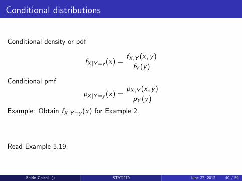
Conditional distributions

Conditional density or pdf

fX |Y=y (x) =fX ,Y (x , y)

fY (y)

Conditional pmf

pX |Y=y (x) =pX ,Y (x , y)

pY (y)

Example: Obtain fX |Y=y (x) for Example 2.

Read Example 5.19.


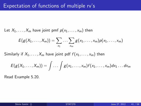
Expectation of functions of multiple rv’s

Let X1, . . . ,Xm have joint pmf p(x1, . . . , xm) then

E (g(X1, . . . ,Xm)) =∑x1

. . .∑xm

g(x1, . . . , xm)p(x1, . . . , xm)

Similarly if X1, . . . ,Xm have joint pdf f (x1, . . . , xm) then

E (g(X1, . . . ,Xm)) =

∫. . .

∫g(x1, . . . , xm)f (x1, . . . , xm)dx1 . . . dxm

Read Example 5.20.


Example 5.21

Suppose X and Y are independent with pdf’s fX (x) = 3x2, 0 < x < 1 andfY (2y), 0 < y < 1 respectively. Obtain E (|X − Y |).


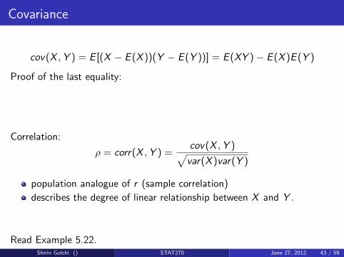
Covariance

cov(X ,Y ) = E [(X − E (X ))(Y − E (Y ))] = E (XY )− E (X )E (Y )

Proof of the last equality:

Correlation:

ρ = corr(X ,Y ) =cov(X ,Y )√var(X )var(Y )

population analogue of r (sample correlation)

describes the degree of linear relationship between X and Y .

Read Example 5.22.Shirin Golchi () STAT270 June 27, 2012 43 / 59

Remark: If X and Y are independent rv’s then

cov(X ,Y ) = corr(X ,Y ) = 0

Proof: page 97

Proposition: X and Y rv’s,

E (a1X + a2Y + b) = a1E (X ) + a2E (Y ) + b

var(a1X + a2Y + b) = a21var(X ) + a2

2var(Y ) + 2a1a2cov(X ,Y )

Proof: page 98

Generalization to m rv’s X1, . . . ,Xm,

E (m∑i=1

aiXi + b) =m∑i=1

aiE (Xi ) + b

var(m∑i=1

aiXi + b) =m∑i=1

a2i var(Xi ) + 2

∑i<j

aiajcov(Xi ,Xj)


Statistics

Definition: A statistic is a function of data, e.g., x̃ , x̄ , s2, x(1) etc.

does not depend on unknown parameters

X1, . . . ,Xn random ⇒ Q(X1, . . . ,Xn) randomx1, . . . , xm a realization of X1, . . . ,Xn ⇒ Q(x1, . . . , xn) a realizationof Q(X1, . . . ,Xn), e.g., x̄ is a realization of X̄


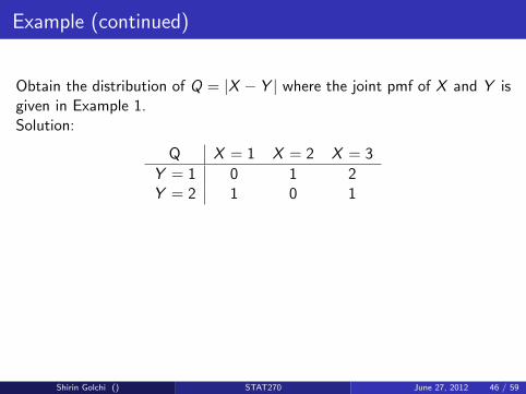
Example (continued)

Obtain the distribution of Q = |X − Y | where the joint pmf of X and Y isgiven in Example 1.Solution:

Q X = 1 X = 2 X = 3

Y = 1 0 1 2Y = 2 1 0 1


Distribution of statistics

Discrete case,pQ(q) =

∑. . .∑A

p(x1, . . . , xm)

Continuous case,

fQ(q) =

∫. . .

∫Ap(x1, . . . , xm)dx1 . . . dxm

where A = {(x1, . . . , xm) : Q(x1, . . . , xm) = q}.

Usually not easy to derive

The distribution is studied using simulation


Simulation

1 Generate N copies of the sample x1, . . . , xn from its distribution

2 Evaluate Q(x1, . . . , xn) for each sample to get q1, . . . , qN which are Nvalues generated from the distribution of Q.

3 Draw histograms, calculate summary statistics, etc.

Example: X ∼ N(0, 1), Y ∼ N(0, 1), Q = |X − Y |.Histogram of x

x

Freq

uenc

y

−3 −2 −1 0 1 2 3

050

100

150

200

Histogram of y

y

Freq

uenc

y

−3 −2 −1 0 1 2 3

050

100

150

Histogram of q

q

Freq

uenc

y

0 1 2 3 4

050

100

150

200

250


iid rv’s

X1, . . . ,Xn independent and identically distributed (iid)

Random sample: A realization of X1, . . . ,Xn: x1, . . . , xm

Example: Let X1, . . . ,Xn be iid with E (Xi ) = µ and var(Xi ) = σ2 then

E (X̄ ) = µ

and

var(X̄ ) =σ2

n

(less variation in X̄ than in Xi s).

X1, . . . ,Xn iid N(µ, σ2) ⇒ X̄ ∼ N(µ, σ2

n )


Example

Linear combinations of normal random variables are normal randomvariables.

Let X , Y , Z be independent with distributions N(1, 12 ), N(0, 3

2 ) andN(1, 3

2 ) respectively. What is the distribution of W = 2X + Y − Z?


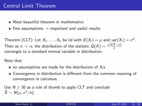
Central Limit Theorem

Most beautiful theorem in mathematics

Few assumptions → important and useful results

Theorem (CLT): Let X1, . . . ,Xn be iid with E (Xi ) = µ and var(Xi ) = σ2.

Then as n→∞ the distribution of the statistic Q(X ) =√n(X̄−µ)σ

converges to a standard normal variable in distribution.

Note that:

no assumptions are made for the distribution of Xi s.

Convergence in distribution is different from the common meaning ofconvergence in calculous.

Use N ≥ 30 as a rule of thumb to apply CLT and concludeX̄ ∼ N(µ, σ2/n).


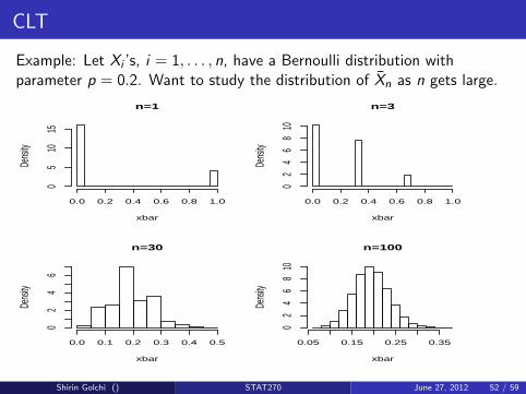
CLT

Example: Let Xi ’s, i = 1, . . . , n, have a Bernoulli distribution withparameter p = 0.2. Want to study the distribution of X̄n as n gets large.

n=1

xbar

Dens

ity

0.0 0.2 0.4 0.6 0.8 1.0

05

1015

n=3

xbar

Dens

ity

0.0 0.2 0.4 0.6 0.8 1.0

02

46

810

n=30

xbar

Dens

ity

0.0 0.1 0.2 0.3 0.4 0.5

02

46

n=100

xbar

Dens

ity

0.05 0.15 0.25 0.35

02

46

810


Example

Suppose the human body weight average is 75kg with variance 400kg2. Ahospital elevator has a maximum load of 3000kg . If 40 people are takingthe elevator what is the probability that the maximum load is exceeded?


Example

An Instructor gives a quiz with two parts. For a randomly selected studentlet X and Y be the scores obtained on the two parts respectively. Thejoint pmf of X and Y is given below:

p(x , y) y = 0 y = 5 y = 10 y = 15

x = 0 .02 .06 .02 .1x = 5 .04 .15 .2 .1x = 10 .01 .15 .14 .01

(a) What is the expected total score E (X + Y )?(b) What is the expected maximum score from the two parts?(c) Are x and Y independent?(d) Obtain P(Y = 10|X ≥ 5).


Example

Suppose X1 ∼ N(1, .25) and X2 ∼ N(2, 25) and corr(X1,X2) = 0.8.Obtain distribution of Y = X1 − X2.


Example

Suppose that the waiting time for a bus in the morning is uniformlydistributed on [0, 8] whereas the waiting time for a bus in the evening isuniformly distributed on [0, 10]. Assume that the waiting times areindependent.(a) If you take a bus each morning and evening for a week, what is thetotal expected waiting time?(b) What is the variance of the total waiting time?(c) What are the expected value and variance of how much longer youwait in the evening than in the morning on a given day?


Example

Tim has three errands where Xi is the time required for the ith errand,i = 1, 2, 3, and X4 is the total walking time between errands. Suppose Xi sare independent normal random variables with means µ1 = 15, µ2 = 5,µ3 = 8, µ4 = 12 and sd’s σ1 = 4, σ2 = 1, σ3 = 2, σ4 = 3. If Tim plans toleave his office at 10am and post a note on the door reading ”I will returnby t am”, what time t ensures that the probability of arriving later than tis .01?


Example

Let X1, . . . ,Xn be independent rv’s with a uniform distribution on [a, b].Let Y = max(X1, . . . ,Xn). E (Y ) =?


Example

Suppose that the bus 143 arrival times follow a poisson process with rateλ = 5 per hour. I arrive at the bus stop at 8:30 and meet one of myfriends who tells me that she has already been waiting for the bus for 15minutes. What is the probability that we take the bus no earlier than 8:45?


stat 270 - chapter 5 continuous distributionssgolchi/stat-270/stat270ch5.pdf · stat 270 - chapter...

Documents