starting r

7/18/2019 Starting r

http://slidepdf.com/reader/full/starting-r 1/12

Getting started with R

I. Using R

R is a programming language and software environment for statistical computing and

graphics. It is highly extensible and in recent years has become the most popularlanguage among statisticians for developing and introducing new statisticalmethodology.

R is available on all CUIT computer labs across campus. However, since R is freelyavailable, you will probably want to download it onto your own personal computer. Todownload R go the webpage:

http://www.r-project.org/

and follow the instructions. Let us know if you run into any problems.

Once installed, you can start R by double clicking it’s the desktop icon which opens thefollowing graphical user interface:

When you use the R program it issues a prompt (“>”) where it expects any inputcommands to be made. At this point R is ready to perform statistical analysis on yourdata.



To see which data sets are available in your workspace type the command:

> objects()

Note that if this is the first time you are running R there will be no data on your

workspace.

To get more information about a particular R command you can type:

> help(command_name)

where command_name is the name of the command you are interested in.

Finally, when you are ready to quit R, type the command q() at the prompt:

> q()

At this point you will be asked whether or not you want to save the data from your Rsession. Data which is saved will be available in future R sessions.

II. Getting Started

A. Mathematical Operations

You can perform all the usual mathematical calculations using R, thus making it into aglorified calculator. Here are some examples:

> 2 + 2> 9 - 2> 10*10> 25/5> 3 ^ 2 # Compute 3 to the power of 2.> 100^(1/2)> sqrt(100) # Compute the square root of 100.> log(10) # Compute the natural logarithm of 10.> log10(1000) # Compute the logarithm base 10 of 1000.> exp(1) # Compute e to the power of 1.

> cos(pi/4) # Compute cosine of pi over 4.

B. Vectors and Matrices

R operates on data structures and the simplest such structure is a vector, which is anarray of numbers or characters. You can use R to create vectors and performoperations on them.



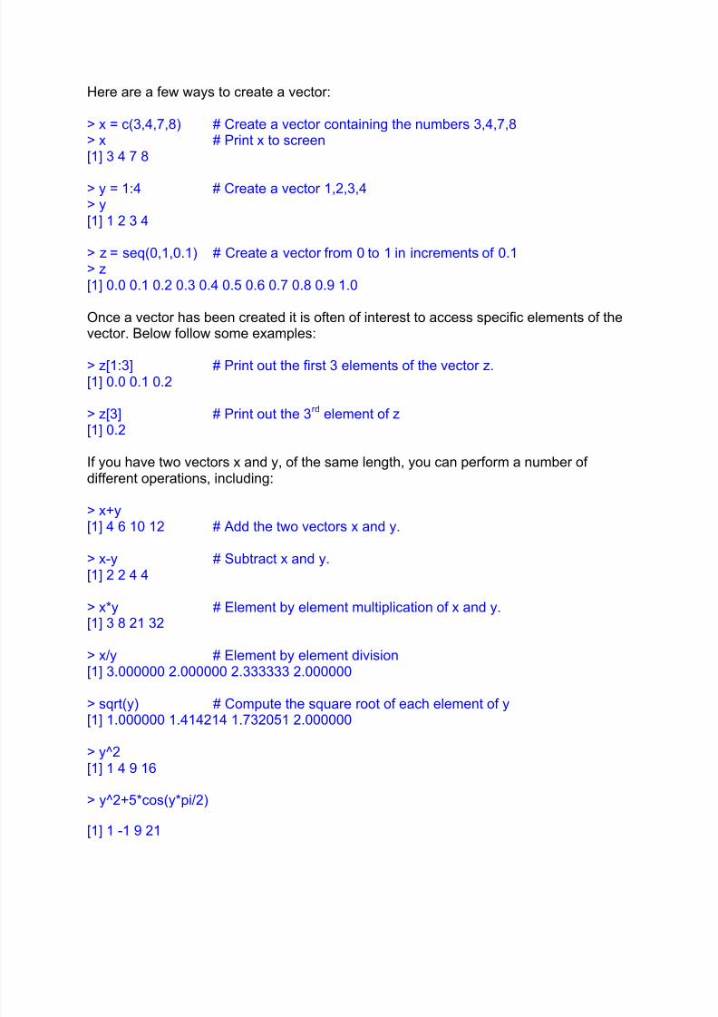
Here are a few ways to create a vector:

> x = c(3,4,7,8) # Create a vector containing the numbers 3,4,7,8> x # Print x to screen[1] 3 4 7 8

> y = 1:4 # Create a vector 1,2,3,4> y[1] 1 2 3 4

> z = seq(0,1,0.1) # Create a vector from 0 to 1 in increments of 0.1> z[1] 0.0 0.1 0.2 0.3 0.4 0.5 0.6 0.7 0.8 0.9 1.0

Once a vector has been created it is often of interest to access specific elements of thevector. Below follow some examples:

> z[1:3] # Print out the first 3 elements of the vector z.[1] 0.0 0.1 0.2

> z[3] # Print out the 3rd element of z[1] 0.2

If you have two vectors x and y, of the same length, you can perform a number ofdifferent operations, including:

> x+y[1] 4 6 10 12 # Add the two vectors x and y.

> x-y # Subtract x and y.[1] 2 2 4 4

> x*y # Element by element multiplication of x and y.[1] 3 8 21 32

> x/y # Element by element division[1] 3.000000 2.000000 2.333333 2.000000

> sqrt(y) # Compute the square root of each element of y[1] 1.000000 1.414214 1.732051 2.000000

> y^2[1] 1 4 9 16

> y^2+5*cos(y*pi/2)

[1] 1 -1 9 21



In R, a vector need not be numerical it can also consist of character elements. To createa vector consisting of the names Bob, Bill, Tom and Sue use the following command:

> names = c("Bob","Bill","Tom","Sue")> names

[1] "Bob" "Bill" "Tom" "Sue"

You can also use R to create matrices:

> X = cbind(x,y) # Combine the vectors x and y into a matrix> Xx y[1,] 3 1[2,] 4 2[3,] 7 3[4,] 8 4

> Y = matrix(0,2,4) # Create a 2x4 matrix with elements equal to 0.> Y[,1] [,2] [,3] [,4][1,] 0 0 0 0[2,] 0 0 0 0

> Z = matrix(x,2,2) # Create a 2x2 matrix with elements equal to x.> Z[,1] [,2][1,] 3 7

[2,] 4 8

To extract the first column of the matrix Z type the command:

> Z[,1][1] 3 4

To extract the second row of the matrix Z type the command:

> Z[2,][1] 4 8

To extract the element contained in the first column of the first row, type the command:

> Z[1,1][1] 3



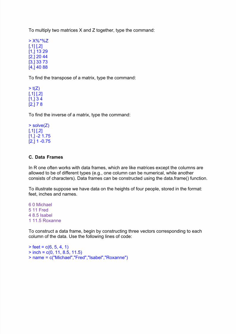
To multiply two matrices X and Z together, type the command:

> X%*%Z[,1] [,2][1,] 13 29

[2,] 20 44[3,] 33 73[4,] 40 88

To find the transpose of a matrix, type the command:

> t(Z)[,1] [,2][1,] 3 4[2,] 7 8

To find the inverse of a matrix, type the command:

> solve(Z)[,1] [,2][1,] -2 1.75[2,] 1 -0.75

C. Data Frames

In R one often works with data frames, which are like matrices except the columns areallowed to be of different types (e.g., one column can be numerical, while anotherconsists of characters). Data frames can be constructed using the data.frame() function.

To illustrate suppose we have data on the heights of four people, stored in the format:feet, inches and names.

6 0 Michael5 11 Fred4 8.5 Isabel1 11.5 Roxanne

To construct a data frame, begin by constructing three vectors corresponding to eachcolumn of the data. Use the following lines of code:

> feet = c(6, 5, 4, 1)> inch = c(0, 11, 8.5, 11.5)> name = c("Michael","Fred","Isabel","Roxanne")



Now the data.frame() function can be used to combine the three vectors into a singledata frame entity.

> Dat = data.frame(feet,inch,name)> Dat

feet inch name1 6 0.0 Michael2 5 11.0 Fred3 4 8.5 Isabel4 1 11.5 Roxanne

Here each row in the data frame will correspond to a different observational unit. Just asin matrix objects, partial information can be easily extracted from the data frame. Toaccess the first row, type:

> Dat[1,]

feet inch name1 6 0 Michael

Suppose now we want to add each person’s weight to the data frame. Adding newvariables is easy to do using the cbind() function as follows:

> weight = c(180, 175, 110, 40)> Dat = cbind(Dat, weight)> Datfeet inch name weight

1 6 0.0 Michael 1802 5 11.0 Fred 1753 4 8.5 Isabel 1104 1 11.5 Roxanne 40

If you prefer entering the data frame in a spreadsheet style data editor, the followingcommand invokes the built-in editor with an empty spreadsheet:

> Dat2 = edit(data.frame())



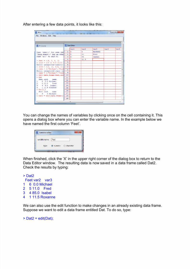
After entering a few data points, it looks like this:

You can change the names of variables by clicking once on the cell containing it. Thisopens a dialog box where you can enter the variable name. In the example below wehave named the first column ‘Feet’.

When finished, click the ‘X’ in the upper right corner of the dialog box to return to theData Editor window. The resulting data is now saved in a data frame called Dat2.Check the results by typing:

> Dat2Feet var2 var3

1 6 0.0 Michael

2 5 11.0 Fred3 4 85.0 Isabel4 1 11.5 Roxanne

We can also use the edit function to make changes in an already existing data frame.Suppose we want to edit a data frame entitled Dat. To do so, type:

> Dat2 = edit(Dat);



An editable spread sheet appears and all changes will be saved in a new data frameentitled Dat2.

III. Accessing Data

A. Reading and Writing Data

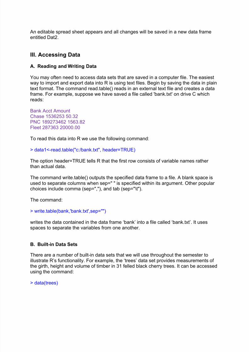
You may often need to access data sets that are saved in a computer file. The easiestway to import and export data into R is using text files. Begin by saving the data in plaintext format. The command read.table() reads in an external text file and creates a dataframe. For example, suppose we have saved a file called 'bank.txt' on drive C whichreads:

Bank Acct AmountChase 1536253 50.32

PNC 189273462 1563.82Fleet 287363 20000.00

To read this data into R we use the following command:

> data1<-read.table("c:/bank.txt", header=TRUE)

The option header=TRUE tells R that the first row consists of variable names ratherthan actual data.

The command write.table() outputs the specified data frame to a file. A blank space is

used to separate columns when sep=" " is specified within its argument. Other popularchoices include comma (sep=","), and tab (sep="\t").

The command:

> write.table(bank,'bank.txt',sep="")

writes the data contained in the data frame ‘bank’ into a file called ‘bank.txt’. It usesspaces to separate the variables from one another.

B. Built-in Data Sets

There are a number of built-in data sets that we will use throughout the semester toillustrate R’s functionality. For example, the ‘trees’ data set provides measurements ofthe girth, height and volume of timber in 31 felled black cherry trees. It can be accessedusing the command:

> data(trees)



> treesGirth Height Volume

1 8.3 70 10.32 8.6 65 10.33 8.8 63 10.2!!

30 18.0 80 51.031 20.6 87 77.0

If we want to access the variable named ‘Girth’ in data frame ‘trees’ we need to type:

> trees$Girth[1] 8.3 8.6 8.8 10.5 10.7 10.8 11.0 11.0 11.1 11.2 11.3 11.4 11.4 11.7 12.0

[16] 12.9 12.9 13.3 13.7 13.8 14.0 14.2 14.5 16.0 16.3 17.3 17.5 17.9 18.0 18.0[31] 20.6

In the long run it becomes unwieldy to call on variables in this manner (i.e., using $). Wecan avoid this by attaching the data to the R search path. This allows objects in thedatabase to be accessed by simply giving their names.

> attach(trees)> Girth[1] 8.3 8.6 8.8 10.5 10.7 10.8 11.0 11.0 11.1 11.2 11.3 11.4 11.4 11.7 12.0

[16] 12.9 12.9 13.3 13.7 13.8 14.0 14.2 14.5 16.0 16.3 17.3 17.5 17.9 18.0 18.0[31] 20.6

When you are finished working without a data set type:

> detach(trees)

IV. Graphics

One of the best things about R is its flexibility in making graphics. Here we will discusshow to make simple histograms, boxplots and scatterplots. To illustrate we will use the‘trees’ data set introduced above.

> data(trees)

> attach(trees)

To make a boxplot of the data in the variable Volume, type:

> hist(Volume)



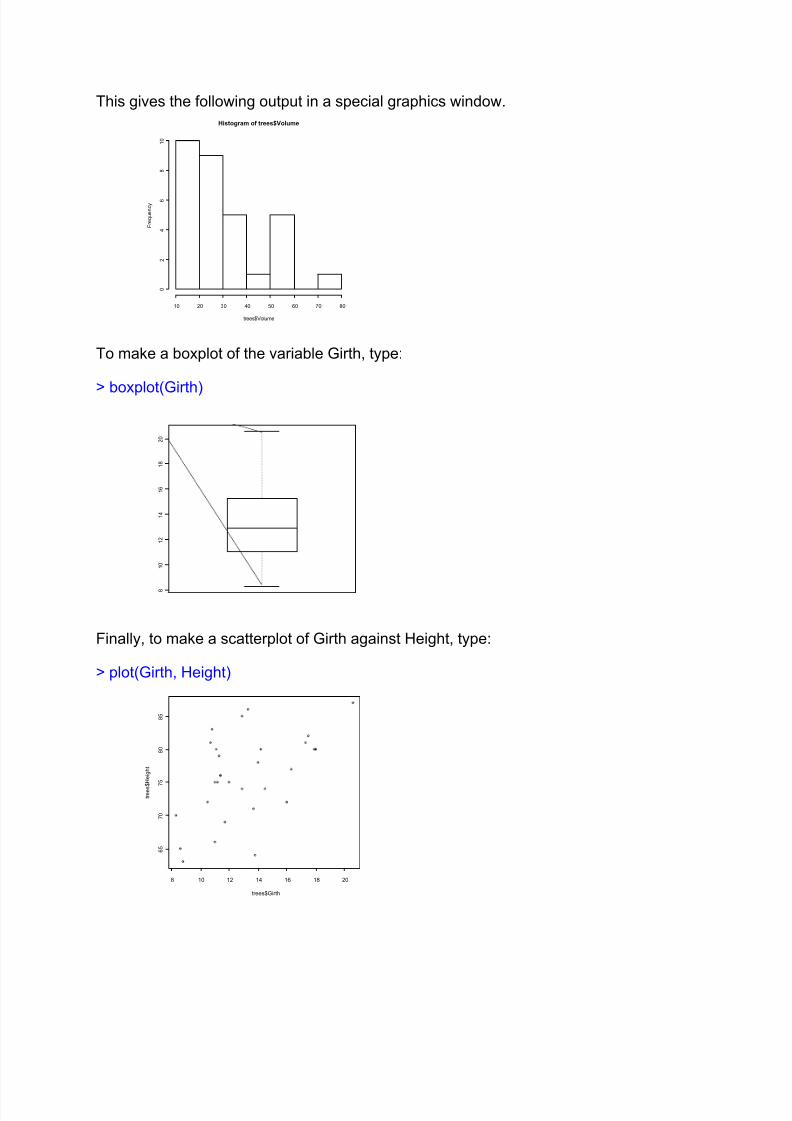
This gives the following output in a special graphics window.

To make a boxplot of the variable Girth, type:

> boxplot(Girth)

Finally, to make a scatterplot of Girth against Height, type:

> plot(Girth, Height)

Histogram of trees$Volume

trees$Volume

F r e q u e n c y

10 20 30 40 50 60 70 80

0

2

4

6

8

1 0

8

1 0

1 2

1 4

1 6

1 8

2 0

8 10 12 14 16 18 20

6 5

7 0

7

5

8 0

8 5

trees$Girth

t r e e s $

H e i g h t



Each of these plot types have multiple options that can be used to make the graphsmore aesthetically pleasing. We will explore these options as the semester progresses.

There are two different ways to save a graph in R. To save the graph as a metafile orbitmap, simply right-click on the graph and a menu will appear. Copy the graph as a

metafile or bitmap and then paste the graph into an editor. You may also choose tosave the graph by going to the pull down window ‘File’ and pressing ‘Save as!...’.

V. Descriptive statistics

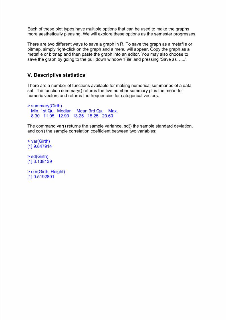
There are a number of functions available for making numerical summaries of a dataset. The function summary() returns the five number summary plus the mean fornumeric vectors and returns the frequencies for categorical vectors.

> summary(Girth)

Min. 1st Qu. Median Mean 3rd Qu. Max.8.30 11.05 12.90 13.25 15.25 20.60

The command var() returns the sample variance, sd() the sample standard deviation,and cor() the sample correlation coefficient between two variables:

> var(Girth)[1] 9.847914

> sd(Girth)[1] 3.138139

> cor(Girth, Height)[1] 0.5192801



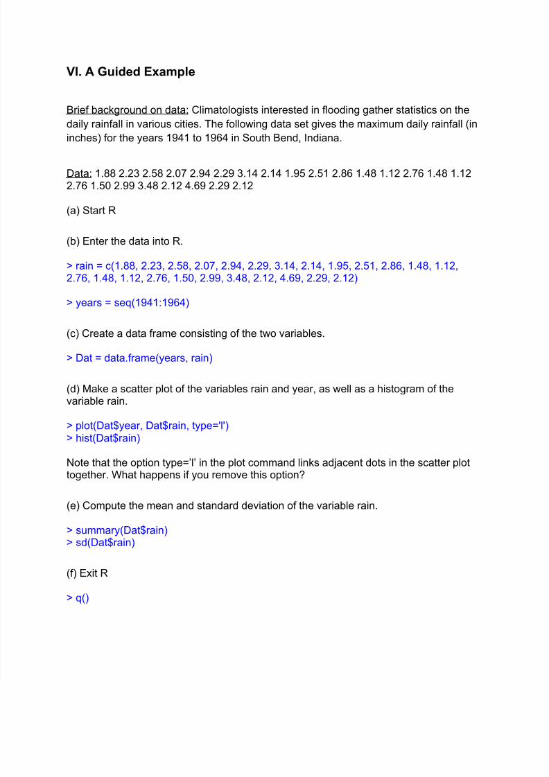
VI. A Guided Example

Brief background on data: Climatologists interested in flooding gather statistics on the

daily rainfall in various cities. The following data set gives the maximum daily rainfall (in

inches) for the years 1941 to 1964 in South Bend, Indiana.

Data: 1.88 2.23 2.58 2.07 2.94 2.29 3.14 2.14 1.95 2.51 2.86 1.48 1.12 2.76 1.48 1.122.76 1.50 2.99 3.48 2.12 4.69 2.29 2.12

(a) Start R

(b) Enter the data into R.

> rain = c(1.88, 2.23, 2.58, 2.07, 2.94, 2.29, 3.14, 2.14, 1.95, 2.51, 2.86, 1.48, 1.12,2.76, 1.48, 1.12, 2.76, 1.50, 2.99, 3.48, 2.12, 4.69, 2.29, 2.12)

> years = seq(1941:1964)

(c) Create a data frame consisting of the two variables.

> Dat = data.frame(years, rain)

(d) Make a scatter plot of the variables rain and year, as well as a histogram of thevariable rain.

> plot(Dat$year, Dat$rain, type='l')> hist(Dat$rain)

Note that the option type=’l’ in the plot command links adjacent dots in the scatter plottogether. What happens if you remove this option?

(e) Compute the mean and standard deviation of the variable rain.

> summary(Dat$rain)

> sd(Dat$rain)

(f) Exit R

> q()

starting r

Documents